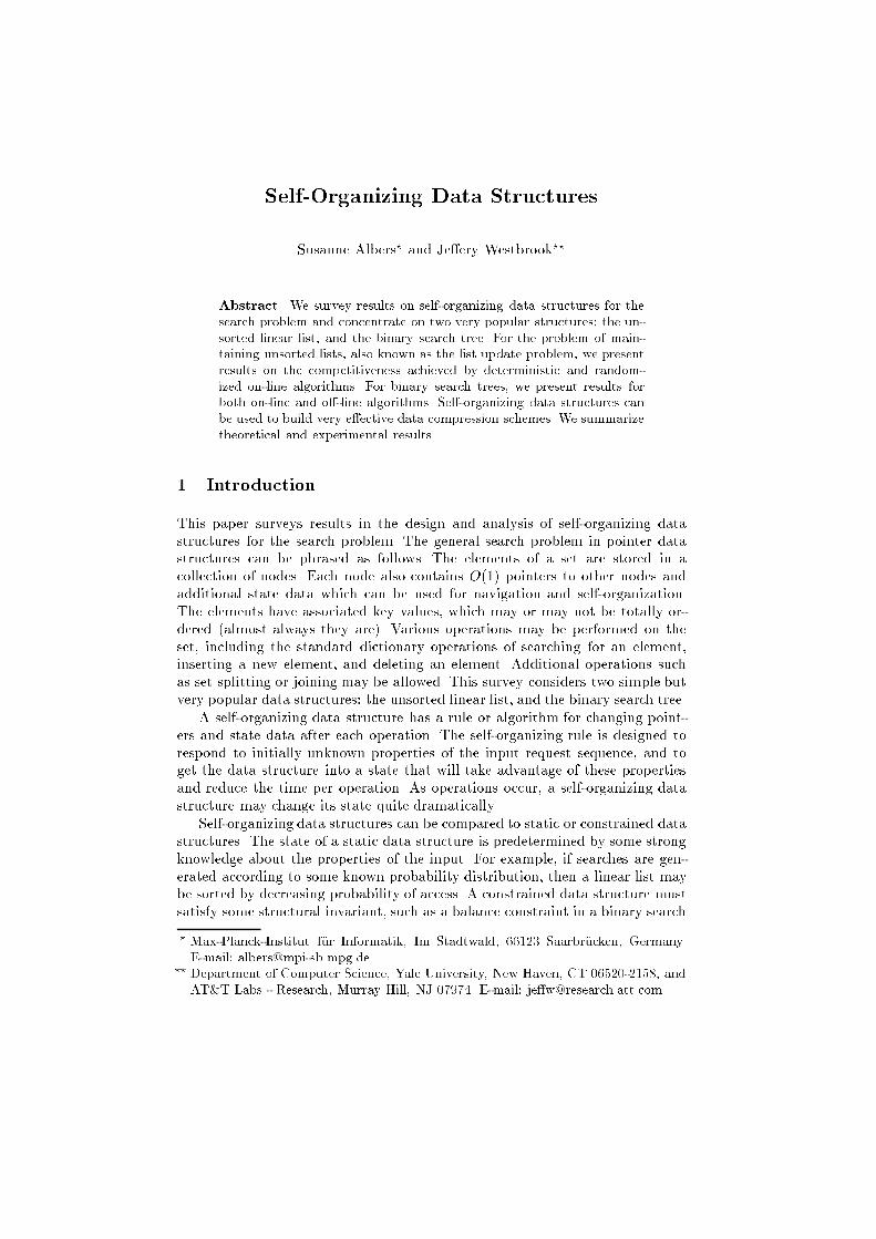
Self-Organizing Data StructuresSusanne Albers? and Je�ery Westbrook??Abstract. We survey results on self-organizing data structures for thesearch problem and concentrate on two very popular structures: the un-sorted linear list, and the binary search tree. For the problem of main-taining unsorted lists, also known as the list update problem, we presentresults on the competitiveness achieved by deterministic and random-ized on-line algorithms. For binary search trees, we present results forboth on-line and o�-line algorithms. Self-organizing data structures canbe used to build very e�ective data compression schemes. We summarizetheoretical and experimental results.1 IntroductionThis paper surveys results in the design and analysis of self-organizing datastructures for the search problem. The general search problem in pointer datastructures can be phrased as follows. The elements of a set are stored in acollection of nodes. Each node also contains O(1) pointers to other nodes andadditional state data which can be used for navigation and self-organization.The elements have associated key values, which may or may not be totally or-dered (almost always they are). Various operations may be performed on theset, including the standard dictionary operations of searching for an element,inserting a new element, and deleting an element. Additional operations suchas set splitting or joining may be allowed. This survey considers two simple butvery popular data structures: the unsorted linear list, and the binary search tree.A self-organizing data structure has a rule or algorithm for changing point-ers and state data after each operation. The self-organizing rule is designed torespond to initially unknown properties of the input request sequence, and toget the data structure into a state that will take advantage of these propertiesand reduce the time per operation. As operations occur, a self-organizing datastructure may change its state quite dramatically.Self-organizing data structures can be compared to static or constrained datastructures. The state of a static data structure is predetermined by some strongknowledge about the properties of the input. For example, if searches are gen-erated according to some known probability distribution, then a linear list maybe sorted by decreasing probability of access. A constrained data structure mustsatisfy some structural invariant, such as a balance constraint in a binary search? Max-Planck-Institut f�ur Informatik, Im Stadtwald, 66123 Saarbr�ucken, Germany.E-mail: albers@mpi-sb.mpg.de.?? Department of Computer Science, Yale University, New Haven, CT 06520-2158, andAT&T Labs - Research, Murray Hill, NJ 07974. E-mail: je�w@research.att.com.

tree. As long as the structural invariant is satis�ed, the data structure does notchange.Self-organizing data structures have several advantages over static and con-strained data structures [64]. (a) The amortized asymptotic time of search andupdate operations is usually as good as the corresponding time of constrainedstructures. But when the sequence of operations has favorable properties, theperformance can be much better. (b) Self-organizing rules need no knowledgeof the properties of input sequence, but will adapt the data structure to bestsuit the input. (c) The self-organizing rule typically results in search and updatealgorithms that are simple and easy to implement. (d) Often the self-organizingrule can be implemented without using any extra space in the nodes. (Such a ruleis called \memoryless" since it saves no information to help make its decisions.)On the other hand, self-organizing data structures have several disadvan-tages. (a) Although the total time of a sequence of operations is low, an indi-vidual operation can be quite expensive. (b) Reorganization of the structure hasto be done even during search operations. Hence self-organizing data structuresmay have higher overheads than their static or constraint-based cousins.Nevertheless, self-organizing data structures represent an attractive alter-native to constraint structures, and reorganization rules have been studied ex-tensively for both linear lists and binary trees. Both data structures have alsoreceived considerable attention within the study of on-line algorithms. In Sec-tion 2 we review results for linear lists. Almost all previous work in this area hasconcentrated on designing on-line algorithms for this data structure. In Section 3we discuss binary search trees and present results on on-line and o�-line algo-rithms. Self-organizing data structures can be used to construct e�ective datacompression schemes. We address this application in Section 4.2 Unsorted linear listsThe problem of representing a dictionary as an unsorted linear list is also knownas the list update problem. Consider a set S of items that has to be maintainedunder a sequence of requests, where each request is one of the following opera-tions.Access(x). Locate item x in S.Insert(x). Insert item x into S.Delete(x). Delete item x from S.Given that S shall be represented as an unsorted list, these operations can beimplemented as follows. To access an item, a list update algorithm starts at thefront of the list and searches linearly through the items until the desired itemis found. To insert a new item, the algorithm �rst scans the entire list to verifythat the item is not already present and then inserts the item at the end of thelist. To delete an item, the algorithm scans the list to search for the item andthen deletes it.In serving requests a list update algorithm incurs cost. If a request is anaccess or a delete operation, then the incurred cost is i, where i is the position of2

the requested item in the list. If the request is an insertion, then the cost is n+1,where n is the number of items in the list before the insertion. While processinga request sequence, a list update algorithm may rearrange the list. Immediatelyafter an access or insertion, the requested item may be moved at no extra costto any position closer to the front of the list. These exchanges are called freeexchanges. Using free exchanges, the algorithm can lower the cost on subsequentrequests. At any time two adjacent items in the list may be exchanged at a costof 1. These exchanges are called paid exchanges.The cost model de�ned above is called the standard model. Manasse et al. [53]and Reingold et al. [61] introduced the P d cost model. In the P d model thereare no free exchanges and each paid exchange costs d. In this survey, we willpresent results both for the standard and the P d model. However, unless other-wise stated, we will always assume the standard cost model.We are interested in list update algorithms that serve a request sequence sothat the total cost incurred on the entire sequence is as small as possible. Ofparticular interest are on-line algorithms, i.e., algorithms that serve each requestwithout knowledge of any future requests. In [64], Sleator and Tarjan suggestedcomparing the quality of an on-line algorithm to that of an optimal o�-linealgorithm. An optimal o�-line algorithm knows the entire request sequence inadvance and can serve it with minimum cost. Given a request sequence �, letCA(�) denote the cost incurred by an on-line algorithm A in serving �, and letCOPT (�) denote the cost incurred by an optimal o�-line algorithm OPT. Thenthe on-line algorithm A is called c-competitive if there is a constant a such thatfor all size lists and all request sequences �,CA(�) � c �COPT (�) + a:The factor c is also called the competitive ratio. Here we assume that A is adeterministic algorithm.The competitive ratio of a randomized on-line algorithmhas to be de�ned in a more careful way, see Section 2.2. In Sections 2.1 and 2.2 wewill present results on the competitiveness that can be achieved by deterministicand randomized on-line algorithms.At present it is unknown whether the problem of computing an optimal wayto process a given request sequence is NP-hard. The fastest optimal o�-linealgorithm currently known is due to Reingold and Westbrook [60] and runs intime O(2nn!m), where n is the size of the list and m is the length of the requestsequence.Linear lists are one possibility to represent a dictionary. Certainly, thereare other data structures such as balanced search trees or hash tables that,depending on the given application, can maintain a dictionary in a more e�cientway. In general, linear lists are useful when the dictionary is small and consistsof only a few dozen items [15]. Furthermore, list update algorithms have beenused as subroutines in algorithms for computing point maxima and convex hulls[14,31]. Recently, list update techniques have been very successfully applied inthe development of data compression algorithms [18]. We discuss this applicationin detail in Section 4. 3

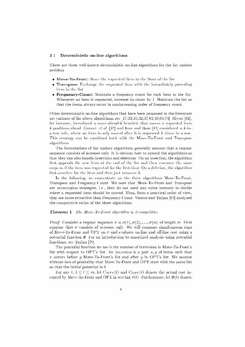
2.1 Deterministic on-line algorithmsThere are three well-known deterministic on-line algorithms for the list updateproblem.� Move-To-Front: Move the requested item to the front of the list.� Transpose: Exchange the requested item with the immediately precedingitem in the list.� Frequency-Count: Maintain a frequency count for each item in the list.Whenever an item is requested, increase its count by 1. Maintain the list sothat the items always occur in nonincreasing order of frequency count.Other deterministic on-line algorithms that have been proposed in the literatureare variants of the above algorithms, see [17,32,35,42,47,62,40,64,74]. Rivest [62],for instance, introduced a move-ahead-k heuristic that moves a requested itemk positions ahead. Gonnet et al. [32] and Kan and Ross [41] considered a k-in-a-row rule, where an item is only moved after it is requested k times in a row.This strategy can be combined both with the Move-To-Front and Transposealgorithms.The formulations of list update algorithms generally assume that a requestsequence consists of accesses only. It is obvious how to extend the algorithms sothat they can also handle insertions and deletions. On an insertion, the algorithm�rst appends the new item at the end of the list and then executes the samesteps as if the item was requested for the �rst time. On a deletion, the algorithm�rst searches for the item and then just removes it.In the following, we concentrate on the three algorithms Move-To-Front,Transpose and Frequency-Count. We note that Move-To-Front and Transposeare memoryless strategies, i.e., they do not need any extra memory to decidewhere a requested item should be moved. Thus, from a practical point of view,they are more attractive than Frequency-Count. Sleator and Tarjan [64] analyzedthe competitive ratios of the three algorithms.Theorem 1. The Move-To-Front algorithm is 2-competitive.Proof. Consider a request sequence � = �(1); �(2); : : : ; �(m) of length m. Firstsuppose that � consists of accesses only. We will compare simultaneous runsof Move-To-Front and OPT on � and evaluate on-line and o�-line cost using apotential function �. For an introduction to amortized analysis using potentialfunctions, see Tarjan [70].The potential function we use is the number of inversions in Move-To-Front'slist with respect to OPT's list. An inversion is a pair x; y of items such thatx occurs before y Move-To-Front's list and after y in OPT's list. We assumewithout loss of generality that Move-To-Front and OPT start with the same listso that the initial potential is 0.For any t, 1 � t � m, let CMTF (t) and COPT (t) denote the actual cost in-curred by Move-To-Front and OPT in serving �(t). Furthermore, let �(t) denote4

the potential after �(t) is served. The amortized cost incurred by Move-To-Fronton �(t) is de�ned as CMTF (t) + �(t)� �(t� 1). We will show that for any t,CMTF (t) + �(t)� �(t� 1) � 2COPT (t) � 1: (1)Summing this expression for all t we obtain Pmt=1CMTF (t) + �(m) � �(0) �Pmt=1 2COPT (t)�m, i.e., CMTF (�) � 2COPT (�)�m+ �(0)� �(m). Since theinitial potential is 0 and the �nal potential is non-negative, the theorem follows.In the following we will show inequality (1) for an arbitrary t. Let x bethe item requested by �(t). Let k denote the number of items that precede xin Move-To-Front's and OPT's list. Furthermore, let l denote the number ofitems that precede x in Move-To-Front's list but follow x in OPT's list. We haveCMTF (t) = k + l + 1 and COPT (t) � k + 1.When Move-To-Front serves �(t) and moves x to the front of the list, linversions are destroyed and at most k new inversions are created. ThusCMTF (t) + �(t)� �(t� 1) � CMTF (t) + k � l = 2k+ 1� 2COPT (t)� 1:Any paid exchange made by OPT when serving �(t) can increase the potentialby 1, but OPT also pays 1. We conclude that inequality (1) holds.The arguments above can be extended easily to analyze an insertion or dele-tion. On an insertion, CMTF (t) = COPT (t) = n + 1, where n is the number ofitems in the list before the insertion, and at most n new inversions are created.On a deletion, l inversions are removed and no new inversion is created. 2Bentley and McGeoch [15] proved a weaker version of Theorem 1. Theyshowed that on any sequence of accesses, the cost incurred by Move-To-Front isat most twice the cost of the optimum static o�-line algorithm. The optimumstatic o�-line algorithm �rst arranges the items in order of decreasing requestfrequencies and does no further exchanges while serving the request sequence.The proof of Theorem 1 shows that Move-To-Front is (2 � 1n)-competitive,where n is the maximum number of items ever contained in the dictionary.Irani [37] gave a re�ned analysis of the Move-To-Front rule and proved that itis (2� 2n+1 )-competitive.Sleator and Tarjan [64] showed that, in terms of competitiveness, Move-To-Front is superior to Transpose and Frequency-Count.Proposition 2. The algorithms Transpose and Frequency-Count are not c-com-petitive for any constant c.Recently, Albers [4] presented another deterministic on-line algorithm forthe list update problem. The algorithm belongs to the Timestamp(p) family ofalgorithms that were introduced in the context of randomized on-line algorithmsand that are de�ned for any real number p 2 [0; 1]. For p = 0, the algorithm isdeterministic and can be formulated as follows.Algorithm Timestamp(0): Insert the requested item, say x, in front of the�rst item in the list that precedes x in the list and that has been requested at5

most once since the last request to x. If there is no such item or if x has notbeen requested so far, then leave the position of x unchanged.Theorem 3. The Timestamp(0) algorithm is 2-competitive.Note that Timestamp(0) is not memoryless. We need information on past re-quests in order to determine where a requested item should be moved. In fact, inthe most straightforward implementation of the algorithmwe need a second passthrough the list to �nd the position where the accessed item must be inserted.Often, such a second pass through the list does not harm the bene�t of a listupdate algorithm. When list update algorithms are applied in the area of datacompression, the positions of the accessed items are of primary importance, seeSection 4.The Timestamp(0) algorithm is interesting because it has a better overallperformance than Move-To-Front. The algorithm achieves a competitive ratioof 2, as does Move-To-Front. However, as we shall see in Section 2.3, Time-stamp(0) is considerably better than Move-To-Front on request sequences thatare generated by probability distributions.El-Yaniv [29] recently presented a new family of deterministic on-line algo-rithms for the list update problem. This family also contains the algorithmsMove-To-Front and Timestamp(0). The following algorithm is de�ned for everyinteger k � 1.Algorithm MRI(k): Insert the requested item, say x, just after the last itemin the list that precedes x in the list and was requested at least k+1 times sincethe last request to x. If there is no such item or if x has not been requested sofar, then move x to the front of the list.El-Yaniv [29] showed that MRI(1) and TIMESTAMP(0) are equivalent andalso proved the following theorem.Theorem 4. For every integer k � 1, the MRI(k) algorithm is 2-competitive.Bachrach and El-Yaniv [10] recently presented an extensive experimentalstudy of list update algorithms. The request sequences used were derived fromthe Calgary Compression Corpus [77]. In many cases, members of the MRI familywere among the best algorithms.Karp and Raghavan [42] developed a lower bound on the competitiveness thatcan be achieved by deterministic on-line algorithms. This lower bound impliesthat Move-To-Front, Timestamp(0) and MRI(k) have an optimal competitiveratio.Theorem 5. Let A be a deterministic on-line algorithm for the list update prob-lem. If A is c-competitive, then c � 2.Proof. Consider a list of n items.We construct a request sequence that consists ofaccesses only. Each request is made to the item that is stored at the last positionin A's list. On a request sequence � of length m generated in this way, A incursa cost of CA(�) = mn. Let OPT0 be the optimum static o�-line algorithm. OPT06

�rst sorts the items in the list in order of nonincreasing request frequencies andthen serves � without making any further exchanges. When rearranging the list,OPT0 incurs a cost of at most n(n� 1)=2. Then the requests in � can be servedat a cost of at most m(n + 1)=2. Thus COPT (�) � m(n+1)=2+n(n� 1)=2. Forlong request sequences, the additive term of n(n�1)=2 can be neglected and weobtain CA(�) � 2nn+1 �COPT (�):The theorem follows because the competitive ratio must hold for all list lengths.2The proof shows that the lower bound is actually 2� 2n+1 , where n is the numberof items in the list. Thus, the upper bound given by Irani on the competitiveratio of the Move-To-Front rule is tight.Next we consider list update algorithms for other cost models. Reingold etal. [61] gave a lower bound on the competitiveness achieved by deterministicon-line algorithms.Theorem 6. Let A be a deterministic on-line algorithm for the list update prob-lem in the P d model. If A is c-competitive, then c � 3.Below we will give a family of deterministic algorithms for the P d model.The best algorithm in this family achieves a competitive ratio that is approxi-mately 4:56-competitive. We defer presenting this result until the discussion ofrandomized algorithms for the P d model, see Section 2.2.Sleator and Tarjan considered another generalized cost model. Let f be anondecreasing function from the positive integers to the nonnegative reals. Sup-pose that an access to the i-th item in the list costs f(i) and that an insertioncosts f(n + 1), where n is the number of items in the list before the insertion.Let the cost of a paid exchange of items i and i+ 1 be �f(i) = f(i + 1)� f(i).The function f is convex if �f(i) � �f(i + 1) for all i. Sleator and Tarjan [64]analyzed the Move-To-Front algorithm for convex cost functions. As usual, ndenotes the maximum number of items contained in the dictionary.Theorem 7. If f is convex, thenCMTF (�) � 2 �COPT (�) +Pn�1i=1 (f(n) � f(i))for all request sequences � that consist only of accesses and insertions.The termPn�1i=1 (f(n) � f(i)) accounts for the fact that the initial lists given toMove-To-Front and OPT may be di�erent. If the lists are the same, the term canbe omitted in the inequality. Theorem 7 can be extended to request sequencesthat include deletions if the total cost for deletions does not exceed the totalcost incurred for insertions. Here we assume that a deletion of the i-th item inthe list costs f(i). 7

2.2 Randomized on-line algorithmsThe competitiveness of a randomized on-line algorithm is de�ned with respectto an adversary. Ben-David et al. [13] introduced three kinds of adversaries.They di�er in the way a request sequence is generated and how the adversary ischarged for serving the sequence.� Oblivious Adversary: The oblivious adversary has to generate a completerequest sequence in advance, before any requests are served by the on-line al-gorithm. The adversary is charged the cost of the optimumo�-line algorithmfor that sequence.� Adaptive On-line Adversary: This adversary may observe the on-linealgorithm and generate the next request based on the algorithm's (random-ized) answers to all previous requests. The adversary must serve each requeston-line, i.e., without knowing the random choices made by the on-line algo-rithm on the present or any future request.� Adaptive O�-line Adversary: This adversary also generates a requestsequence adaptively. However, it is charged the optimum o�-line cost forthat sequence.A randomized on-line algorithm A is called c-competitive against any obliv-ious adversary if there is a constant a such that for all size lists and all requestsequences � generated by an oblivious adversary, E[CA(�)] � c � COPT (�) + a:The expectation is taken over the random choices made by A.Given a randomized on-line algorithm A and an adaptive on-line (adaptiveo�-line) adversary ADV, let E[CA] and E[CADV ] denote the expected costsincurred by A and ADV in serving a request sequence generated by ADV. Arandomized on-line algorithm A is called c-competitive against any adaptiveon-line (adaptive o�-line) adversary if there is a constant a such that for allsize lists and all adaptive on-line (adaptive o�-line) adversaries ADV, E[CA] �c � E[CADV ] + a, where the expectation is taken over the random choices madeby A.Ben-David et al. [13] investigated the relative strength of the adversaries withrespect to on-line problems that can be formulated as a request-answer game,see [13] for details. They showed that if there is a randomized on-line algorithmthat is c-competitive against any adaptive o�-line adversary, then there is alsoa c-competitive deterministic on-line algorithm. This immediately implies thatno randomized on-line algorithm for the list update problem can be better than2-competitive against any adaptive o�-line adversary. Reingold et al. [61] proveda similar result for adaptive on-line adversaries.Theorem 8. If a randomized on-line algorithm for the list update problem isc-competitive against any adaptive on-line adversary, then c � 2.The optimal competitive ratio that can be achieved by randomized on-linealgorithms against oblivious adversaries has not been determined yet. In thefollowing we present upper and lower bounds known on this ratio.8

Randomized on-line algorithms against oblivious adversaries The intu-ition behind all randomized on-line algorithms for the list update problem is tomove requested items in a more conservative way than Move-To-Front, which isstill the classical deterministic algorithm.The �rst randomized on-line algorithm for the list update problem was pre-sented by Irani [37,38] and is called Split algorithm.Each item x in the list main-tains a pointer x:split that points to some other item in the list. The pointer ofeach item either points to the item itself or to an item that precedes it in thelist.Algorithm Split: The algorithm works as follows.Initialization:For all items x in the list, set x:split x.If item x is requested:For all items y with y:split = x, set y:split item behind x in the list.With probability 1/2:Move x to the front of the list.With probability 1/2:Insert x before item x:split.If y preceded x and x:split = y:split, then set y:split x.Set x:split to the �rst item in the list.Theorem 9. The Split algorithm is (15=8)-competitive against any obliviousadversary.We note that (15=8) = 1:875. Irani [37,38] showed that the Split algorithm is notbetter than 1.75-competitive in the i� 1 cost model. In the i� 1 cost model, anaccess to the i-th item in the list costs i� 1 rather than i. The i� 1 cost modelis often useful to analyze list update algorithms. Compared to the standardi cost model, where an access to the i-th items costs i, the i � 1 cost modelalways incurs a smaller cost; for any request sequence � and any algorithm A,the cost di�erence is m, where m is the length of �. Thus, a lower bound on thecompetitive ratio developed for a list update algorithm in the i � 1 cost modeldoes not necessarily hold in the i cost model. On the other hand, any upperbound achieved in the i� 1 cost model also holds in the i cost model.A simple and easily implementable list update rule was proposed by Reingoldet al. [61].Algorithm Bit: Each item in the list maintains a bit that is complementedwhenever the item is accessed. If an access causes a bit to change to 1, thenthe requested item is moved to the front of the list. Otherwise the list remainsunchanged. The bits of the items are initialized independently and uniformly atrandom.Theorem 10. The Bit algorithm is 1.75-competitive against any oblivious ad-versary. 9

Reingold et al. analyzed Bit using an elegant modi�cation of the potential func-tion given in the proof of Theorem 1. Again, an inversion is a pair of items x; ysuch that x occurs before y in Bit's list and after y in OPT's list. An inversionhas type 1 if y's bit is 0 and type 2 if y's bit is 1. Now, the potential is de�nedas the number of type 1 inversions plus twice the number of type 2 inversions.The upper bound for Bit is tight in the i � 1 cost model [61]. It was alsoshown that in the i cost model, i.e. in the standard model, Bit is not better than1.625-competitive [3].Reingold et al. [61] gave a generalization of the Bit algorithm. Let l be apositive integer and L be a non-empty subset of f0:1: : : :; l � 1g. The algorithmCounter(l; L) works as follows. Each item in the list maintains a mod l counter.Whenever an item x is accessed, the counter of x is decremented by 1 and,if the new value is in L, the item x is moved to the front of the list. Thecounters of the items are initialized independently and uniformly at randomto some value in f0:1: : : : ; l � 1g. Note that Bit is Counter(2,f1g). Reingold etal. chose parameters l and L so that the resulting Counter(l; L) algorithm isbetter than 1.75-competitive. It is worthwhile to note that the algorithms Bitand Counter(l; L) make random choices only during an initialization phase andrun completely deterministically thereafter.The Counter algorithms can be modi�ed [61]. Consider a Counter(l; f0g)algorithm that is changed as follows. Whenever the counter of an item reaches0, the counter is reset to j with probability pj, 1 � j � l�1. Reingold et al. [61]gave a value for l and a resetting distribution on the pj 's so that the algorithmachieves a competitive ratio of p3 � 1:73.Another family of randomized on-line algorithms was given by Albers [4].The following algorithm works for any real number p 2 [0:1].AlgorithmTimestamp(p): Each request to an item, say x, is served as follows.With probability p execute Step (a).(a) Move x to the front of the list.With probability 1� p execute Step (b).(b) Insert x in front of the �rst item in the list that precedes x and(i) that was not requested since the last request to xor (ii) that was requested exactly once since the last request to x and thecorresponding request was served using Step (b) of the algorithm.If there is no such item or if x is requested for the �rst time, then leave theposition of x unchanged.Theorem 11. For any real number p 2 [0; 1], the algorithm Timestamp(p) isc-competitive against any oblivious adversary, where c = maxf2�p; 1+p(2�p)g.Setting p = (3 �p5)=2, we obtain a �-competitive algorithm, where � = (1 +p5)=2 � 1:62 is the Golden Ratio. The family of Timestamp algorithms alsoincludes two deterministic algorithms. For p = 1, we obtain the Move-To-Frontrule. On the other hand, setting p = 0, we obtain the Timestamp(0) algorithmthat was already described in Section 2.1.10

In order to implement Timestamp(p) we have to maintain, for each item inthe list, the times of the two last requests to that item. If these two times arestored with the item, then after each access the algorithm needs a second passthrough the list to �nd the position where the requested item should be inserted.Note that such a second pass is also needed by the Split algorithm. In the caseof the Split algorithm, this second pass is necessary because pointers have to beupdated.Interestingly, it is possible to combine the algorithms Bit and Timestamp(0),see Albers et al. [6]. This combined algorithm achieves the best competitive ratiothat is currently known for the list update problem.AlgorithmCombination:With probability 4/5 the algorithm serves a requestsequence using Bit, and with probability 1/5 it serves a request sequence usingTimestamp(0).Theorem 12. The algorithm Combination is 1.6-competitive against any obliv-ious adversary.Proof. The analysis consists of two parts. In the �rst part we show that given anyrequest sequence �, the cost incurred by Combination and OPT can be dividedinto costs that are caused by each unordered pair fx; yg of items x and y. Then,in the second part, we compare on-line and o�-line cost for each pair fx; yg. Thismethod of analyzing cost by considering pairs of items was �rst introduced byBentley and McGeoch [15] and later used in [4,37]. In the following we alwaysassume that serving a request to the i-th item in the list incurs a cost of i � 1rather than i. Clearly, if Combination is 1.6-competitive in this i�1 cost model,it is also 1:6-competitive in the i-cost model.Let � = �(1); �(2); : : : ; �(m) be an arbitrary request sequence of length m.For the reduction to pairs we need some notation. Let S be the set of items in thelist. Consider any list update algorithm A that processes �. For any t 2 [1;m]and any item x 2 S, let CA(t; x) be the cost incurred by item x when A serves�(t). More precisely, CA(t; x) = 1 if item x precedes the item requested by �(t)in A's list at time t; otherwise CA(t; x) = 0. If A does not use paid exchanges,then the total cost CA(�) incurred by A on � can be written asCA(�) = Xt2[1;m]Xx2SCA(t; x) =Xx2S Xt2[1;m]CA(t; x)=Xx2SXy2S Xt2[1;m]�(t)=y CA(t; x)= Xfx;ygx6=y ( Xt2[1;m]�(t)=x CA(t; y) + Xt2[1;m]�(t)=y CA(t; x)):For any unordered pair fx; yg of items x 6= y, let �xy be the request sequencethat is obtained from � if we delete all requests that are neither to x nor to y.Let CBIT (�xy) and CTS(�xy) denote the costs that Bit and Timestamp(0) incur11

in serving �xy on a two item list that consist of only x and y. Obviously, if Bitserves � on the long list, then the relative position of x and y changes in thesame way as if Bit serves �xy on the two item list. The same property holdsfor Timestamp(0). This follows from Lemma 13, which can easily be shown byinduction on the number of requests processed so far.Lemma 13. At any time during the processing of �, x precedes y in Time-stamp(0)'s list if and only if one of the following statements holds: (a) the lastrequests made to x and y are of the form xx, xyx or xxy; (b) x preceded yinitially and y was requested at most once so far.Thus, for algorithm A 2 fBit, Timestamp(0)g we haveCA(�xy) = Xt2[1;m]�(t)=x CA(t; y) + Xt2[1;m]�(t)=y CA(t; x)CA(�) = Xfx;ygx6=y CA(�xy): (2)Note that Bit and Timestamp(0) do not incur paid exchanges. For the optimalo�-line cost we haveCOPT (�xy) � Xt2[1;m]�(t)=x COPT (t; y) + Xt2[1;m]�(t)=y COPT (t; x) + p(x; y)and COPT (�) � Xfx;ygx6=y COPT (�xy); (3)where p(x; y) denotes the number of paid exchanges incurred by OPT in movingx in front of y or y in front of x. Here, only inequality signs hold because if OPTserves �xy on the two item list, then it can always arrange x and y optimallyin the list, which might not be possible if OPT serves � on the entire list. Notethat the expected cost E[CCB(�xy)] incurred by Combination on �xy isE[CCB(�xy)] = 45E[CBIT (�xy)] + 15E[CTS(�xy)]: (4)In the following we will show that for any pair fx; yg of items E[CCB(�xy)] �1:6COPT (�xy). Summing this inequality for all pairs fx; yg, we obtain, by equa-tions (2),(3) and (4), that Combination is 1.6-competitive.Consider a �xed pair fx; ygwith x 6= y. We partition the request sequence �xyinto phases. The �rst phase starts with the �rst request in �xy and ends when,for the �rst time, there are two requests to the same item and the next request isdi�erent. The second phase starts with that next request and ends in the sameway as the �rst phase. The third and all remaining phases are constructed in thesame way as the second phase. The phases we obtain are of the following types:12

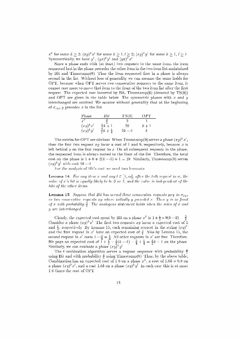
xk for some k � 2; (xy)kxl for some k � 1; l � 2; (xy)kyl for some k � 1, l � 1.Symmetrically, we have yk, (yx)kyl and (yx)kxl.Since a phase ends with (at least) two requests to the same item, the itemrequested last in the phase precedes the other item in the two item list maintainedby Bit and Timestamp(0). Thus the item requested �rst in a phase is alwayssecond in the list. Without loss of generality we can assume the same holds forOPT, because when OPT serves two consecutive requests to the same item, itcannot cost more to move that item to the front of the two item list after the �rstrequest. The expected cost incurred by Bit, Timestamp(0) (denoted by TS(0))and OPT are given in the table below. The symmetric phases with x and yinterchanged are omitted. We assume without generality that at the beginningof �xy, y precedes x in the list.Phase Bit TS(0) OPTxk 32 2 1(xy)kxl 32k + 1 2k k + 1(xy)kyl 32k + 14 2k � 1 kThe entries for OPT are obvious. When Timestamp(0) serves a phase (xy)kxl,then the �rst two request xy incur a cost of 1 and 0, respectively, because x isleft behind y on the �rst request to x. On all subsequent requests in the phase,the requested item is always moved to the front of the list. Therefore, the totalcost on the phase is 1 + 0 + 2(k � 1) + 1 = 2k. Similarly, Timestamp(0) serves(xy)kyl with cost 2k� 1.For the analysis of Bit's cost we need two lemmata.Lemma 14. For any item x and any t 2 [1;m], after the t-th request in �, thevalue of x's bit is equally likely to be 0 or 1, and the value is independent of thebits of the other items.Lemma 15. Suppose that Bit has served three consecutive requests yxy in �xy,or two consecutive requests xy where initially y preceded x. Then y is in frontof x with probability 34 . The analogous statement holds when the roles of x andy are interchanged.Clearly, the expected cost spent by Bit on a phase xk is 1+ 12 +0(k�2) = 32 .Consider a phase (xy)kxl. The �rst two requests xy incur a expected cost of 1and 12 , respectively. By Lemma 15, each remaining request in the string (xy)kand the �rst request in xl have an expected cost of 34 . Also by Lemma 15, thesecond request in xl costs 1� 34 = 14 . All other requests in xl are free. Therefore,Bit pays an expected cost of 1 + 12 + 32 (k � 1) + 34 + 14 = 32k + 1 on the phase.Similarly, we can evaluate a phase (xy)kyl.The Combination algorithm serves a request sequence with probability 45using Bit and with probability 15 using Timestamp(0). Thus, by the above table,Combination has an expected cost of 1.6 on a phase xk, a cost of 1:6k + 0:8 ona phase (xy)kxl, and a cost 1:6k on a phase (xy)kyl. In each case this is at most1.6 times the cost of OPT. 13

In the proof above we assume that a request sequence consists of accessesonly. However, the analysis is easily extended to the case that insertions anddeletions occur, too. For any item x, consider the time intervals during which xis contained in the list. For each of these intervals, we analyze the cost causedby any pair fx; yg, where y is an item that is (temporarily) present during theinterval. 2Teia [72] presented a lower bound for randomized list update algorithms.Theorem 16. Let A be a randomized on-line algorithm for the list update prob-lem. If A is c-competitive against any oblivious adversary, then c � 1:5.An interesting open problem is to give tight bounds on the competitive ratio thatcan be achieved by randomized on-line algorithms against oblivious adversaries.Results in the P d cost model As mentioned in Theorem 6, no deterministicon-line algorithm for the list update problem in the P d model can be betterthan 3-competitive. By a result of Ben-David et al. [13], this implies that norandomized on-line algorithm for the list update problem in the P d model canbe better than 3-competitive against any adaptive o�-line adversary. Reingold etal. [61] showed that the same bound holds against adaptive on-line adversaries.Theorem 17. Let A be a randomized on-line algorithm for the list update prob-lem in the P d model. If A is c-competitive against any adaptive on-line adversary,then c � 3.Reingold et al. [61] analyzed the Counter(l; fl � 1g) algorithms, l being apositive integer, for list update in the P d model. As described before, thesealgorithms work as follows. Each item maintains a mod l counter that is decre-mented whenever the item is requested. When the value of the counter changesto l � 1, then the accessed item is moved to the front of the list. In the P d costmodel, this movement is done using paid exchanges. The counters are initializedindependently and uniformly at random to some value in f0; 1; : : :; l � 1g.Theorem 18. In the P d model, the algorithm Counter(l; fl�1g) is c-competitiveagainst any oblivious adversary, where c = maxf1 + l+12d ; 1 + 1l (2d+ l+12 )g.The best value for l depends on d. As d goes to in�nity, the best competitive ratioachieved by a Counter(l; fl�1g) algorithm decreases and goes to (5+p17)=4 �2:28.We now present an analysis of the deterministic version of the Counter(l; fl�1g) algorithm. The deterministic version is the same as the randomized version,except that all counters are initialized to zero, rather than being randomly ini-tialized.Theorem 19. In the P d model, the deterministic algorithm Counter(l; fl� 1g)is c-competitive, where c = maxf3 + 2ld ; 2 + 2dl g.14

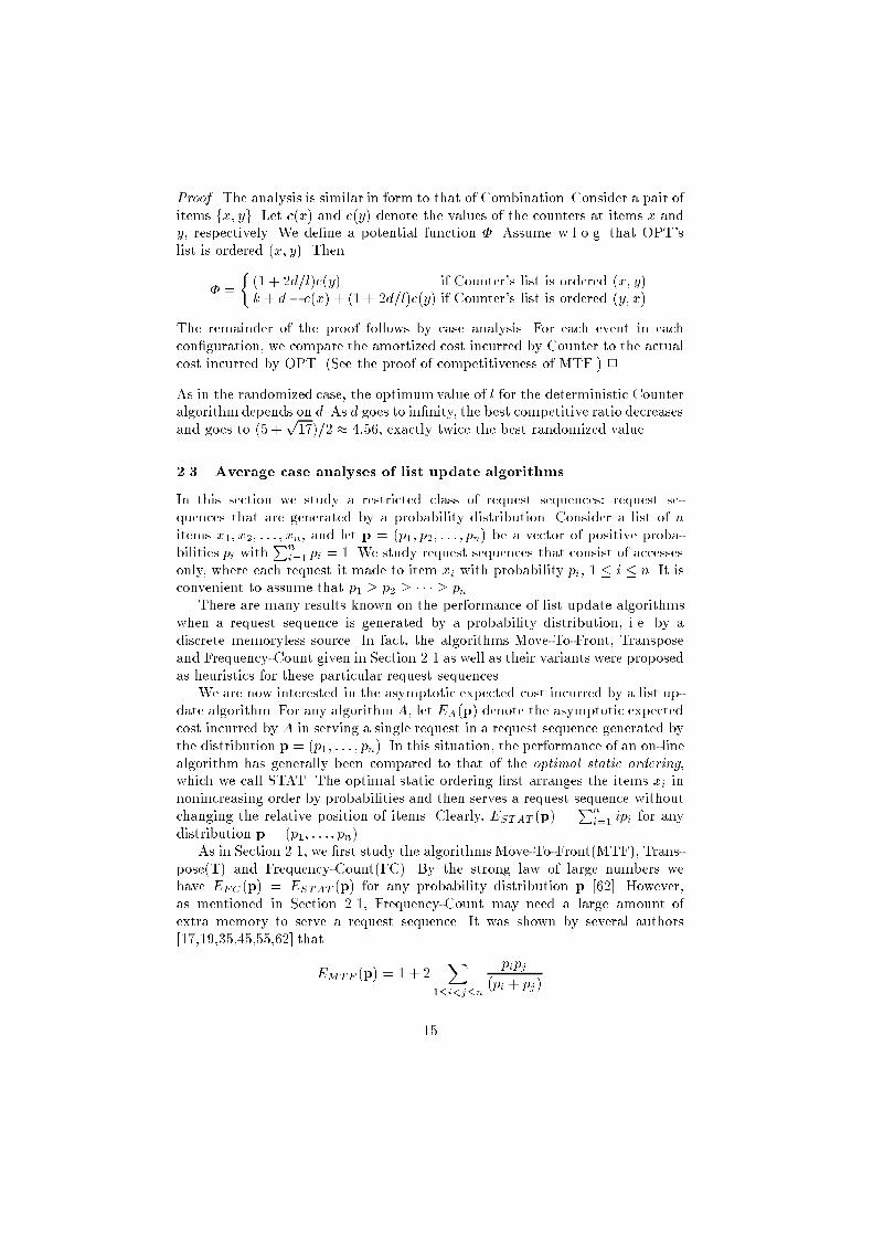
Proof. The analysis is similar in form to that of Combination. Consider a pair ofitems fx; yg. Let c(x) and c(y) denote the values of the counters at items x andy, respectively. We de�ne a potential function �. Assume w.l.o.g. that OPT'slist is ordered (x; y). Then� = � (1 + 2d=l)c(y) if Counter's list is ordered (x; y)k + d� c(x) + (1 + 2d=l)c(y) if Counter's list is ordered (y; x)The remainder of the proof follows by case analysis. For each event in eachcon�guration, we compare the amortized cost incurred by Counter to the actualcost incurred by OPT. (See the proof of competitiveness of MTF.) 2As in the randomized case, the optimum value of l for the deterministic Counteralgorithmdepends on d. As d goes to in�nity, the best competitive ratio decreasesand goes to (5 +p17)=2 � 4:56, exactly twice the best randomized value.2.3 Average case analyses of list update algorithmsIn this section we study a restricted class of request sequences: request se-quences that are generated by a probability distribution. Consider a list of nitems x1; x2; : : : ; xn, and let p = (p1; p2; : : : ; pn) be a vector of positive proba-bilities pi withPni=1 pi = 1. We study request sequences that consist of accessesonly, where each request it made to item xi with probability pi, 1 � i � n. It isconvenient to assume that p1 � p2 � � � � � pn.There are many results known on the performance of list update algorithmswhen a request sequence is generated by a probability distribution, i.e. by adiscrete memoryless source. In fact, the algorithms Move-To-Front, Transposeand Frequency-Count given in Section 2.1 as well as their variants were proposedas heuristics for these particular request sequences.We are now interested in the asymptotic expected cost incurred by a list up-date algorithm. For any algorithmA, let EA(p) denote the asymptotic expectedcost incurred by A in serving a single request in a request sequence generated bythe distribution p = (p1; : : : ; pn). In this situation, the performance of an on-linealgorithm has generally been compared to that of the optimal static ordering,which we call STAT. The optimal static ordering �rst arranges the items xi innonincreasing order by probabilities and then serves a request sequence withoutchanging the relative position of items. Clearly, ESTAT (p) = Pni=1 ipi for anydistribution p = (p1; : : : ; pn).As in Section 2.1, we �rst study the algorithmsMove-To-Front(MTF), Trans-pose(T) and Frequency-Count(FC). By the strong law of large numbers wehave EFC(p) = ESTAT (p) for any probability distribution p [62]. However,as mentioned in Section 2.1, Frequency-Count may need a large amount ofextra memory to serve a request sequence. It was shown by several authors[17,19,35,45,55,62] thatEMTF (p) = 1 + 2 X1�i<j�n pipj(pi + pj)15

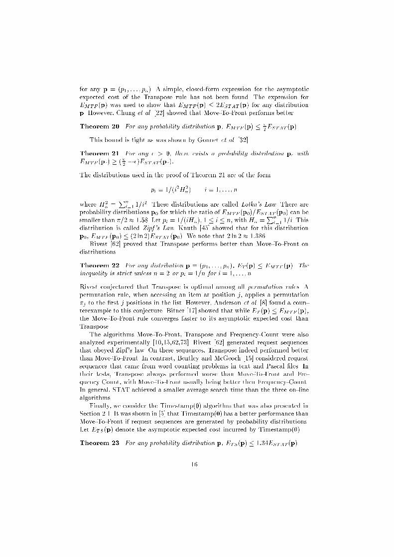
for any p = (p1; : : : ; pn). A simple, closed-form expression for the asymptoticexpected cost of the Transpose rule has not been found. The expression forEMTF (p) was used to show that EMTF (p) � 2ESTAT (p) for any distributionp. However, Chung et al. [22] showed that Move-To-Front performs better.Theorem 20. For any probability distribution p, EMTF (p) � �2ESTAT (p).This bound is tight as was shown by Gonnet et al. [32].Theorem 21. For any � > 0, there exists a probability distribution p� withEMTF (p�) � (�2 � �)ESTAT (p�):The distributions used in the proof of Theorem 21 are of the formpi = 1=(i2H2n) i = 1; : : : ; nwhere H2n = Pni=1 1=i2. These distributions are called Lotka's Law. There areprobability distributions p0 for which the ratio of EMTF (p0)=ESTAT (p0) can besmaller than �=2 � 1:58. Let pi = 1=(iHn), 1 � i � n, withHn =Pni=1 1=i. Thisdistribution is called Zipf's Law. Knuth [45] showed that for this distributionp0, EMTF (p0) � (2 ln2)ESTAT (p0). We note that 2 ln2 � 1:386.Rivest [62] proved that Transpose performs better than Move-To-Front ondistributions.Theorem 22. For any distribution p = (p1; : : : ; pn), ET (p) � EMTF (p). Theinequality is strict unless n = 2 or pi = 1=n for i = 1; : : : ; n.Rivest conjectured that Transpose is optimal among all permutation rules. Apermutation rule, when accessing an item at position j, applies a permutation�j to the �rst j positions in the list. However, Anderson et al. [8] found a coun-terexample to this conjecture. Bitner [17] showed that while ET (p) � EMTF (p),the Move-To-Front rule converges faster to its asymptotic expected cost thanTranspose.The algorithms Move-To-Front, Transpose and Frequency-Count were alsoanalyzed experimentally [10,15,62,73]. Rivest [62] generated request sequencesthat obeyed Zipf's law. On these sequences, Transpose indeed performed betterthan Move-To-Front. In contrast, Bentley and McGeoch [15] considered requestsequences that came from word counting problems in text and Pascal �les. Intheir tests, Transpose always performed worse than Move-To-Front and Fre-quency Count, with Move-To-Front usually being better then Frequency-Count.In general, STAT achieved a smaller average search time than the three on-linealgorithms.Finally, we consider the Timestamp(0) algorithm that was also presented inSection 2.1. It was shown in [5] that Timestamp(0) has a better performance thanMove-To-Front if request sequences are generated by probability distributions.Let ETS(p) denote the asymptotic expected cost incurred by Timestamp(0).Theorem 23. For any probability distribution p, ETS(p) � 1:34ESTAT(p).16

Theorem 24. For any probability distribution p, ETS(p) � 1:5EOPT (p).Note that EOPT (p) is the asymptotic expected cost incurred by the optimal o�-line algorithm OPT, which may dynamically rearrange the list while servinga request sequence. Thus, this algorithm is much stronger than STAT. Thealgorithm Timestamp(0) is the only algorithm whose asymptotic expected costhas been compared to EOPT (p).The bound given in Theorem 24 holds with high probability. More precisely,for every distribution p = (p1; : : : ; pn), and � > 0, there exist constants c1; c2and m0 dependent on p; n and � such that for any request sequence � of lengthm � m0 generated by p,ProbfCTS(�) > (1:5 + �)COPT (�)g � c1e�c2m:2.4 RemarksList update techniques were �rst studied in 1965 by McCabe [55] who consid-ered the problem of maintaining a sequential �le. McCabe also formulated thealgorithms Move-To-Front and Transpose. From 1965 to 1985 the list updateproblem was studied under the assumption that a request sequence is generatedby a probability distribution. Thus, most of the results presented is Section 2.3were developed earlier than the results in Sections 2.1 and 2.2. A �rst survey onlist update algorithms when request sequences are generated by a distributionwas written by Hester and Hirschberg [36]. The paper [64] by Sleator and Tar-jan is a fundamental paper in the entire on-line algorithms literature. It madethe competitive analysis of on-line algorithms very popular. Randomized on-line algorithms for the list update problem have been studied since the earlynineties. The list update problem is a classical on-line problem that continues tobe interesting both from a theoretical and practical point of view.3 Binary search treesBinary search trees are used to maintain a set S of elements where each elementhas an associated key drawn from a totally ordered universe. For convenience weassume each element is given a unique key, and that the n elements have keys1; : : : ; n. We will generally not distinguish between elements and their keys.A binary search tree is a rooted tree in which each node has zero, one, ortwo children. If a node has no left or right child, we say it has a null left or rightchild, respectively. Each node stores an element, and the elements are assignedto the nodes in symmetric order: the element stored in a node is greater than allelements in descendents of its left child, and less than all elements in descendentsof its right child. An inorder traversal of the tree yields the elements in sortedorder. Besides the elements, the nodes may contain additional information usedto maintain states, such as a color bit or a counter.The following operations are commonly performed on binary search trees.17

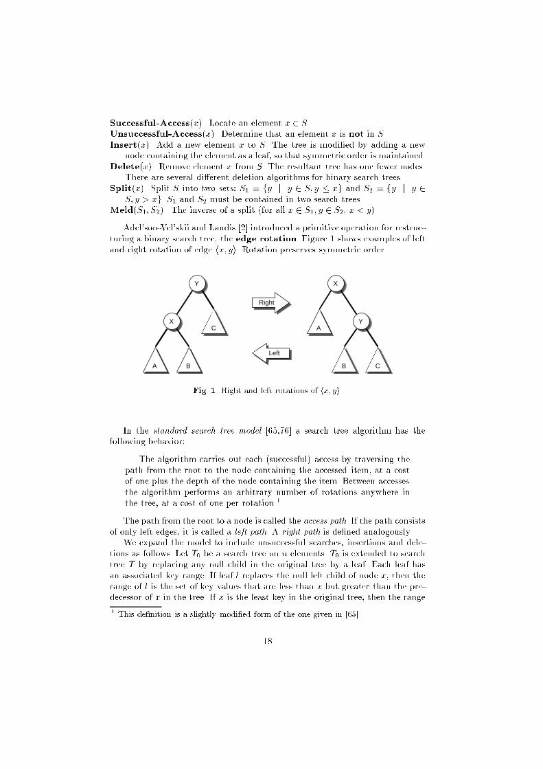
Successful-Access(x). Locate an element x 2 S.Unsuccessful-Access(x). Determine that an element x is not in S.Insert(x). Add a new element x to S. The tree is modi�ed by adding a newnode containing the element as a leaf, so that symmetric order is maintained.Delete(x). Remove element x from S. The resultant tree has one fewer nodes.There are several di�erent deletion algorithms for binary search trees.Split(x). Split S into two sets: S1 = fy j y 2 S; y � xg and S2 = fy j y 2S; y > xg. S1 and S2 must be contained in two search trees.Meld(S1; S2). The inverse of a split (for all x 2 S1; y 2 S2, x < y).Adel'son-Vel'skii and Landis [2] introduced a primitive operation for restruc-turing a binary search tree, the edge rotation. Figure 1 shows examples of leftand right rotation of edge hx; yi. Rotation preserves symmetric order.X

A

Y

B

CY

X

CB

A

Right

LeftFig. 1. Right and left rotations of hx; yi.In the standard search tree model [65,76] a search tree algorithm has thefollowing behavior:The algorithm carries out each (successful) access by traversing thepath from the root to the node containing the accessed item, at a costof one plus the depth of the node containing the item. Between accessesthe algorithm performs an arbitrary number of rotations anywhere inthe tree, at a cost of one per rotation.1The path from the root to a node is called the access path. If the path consistsof only left edges, it is called a left path. A right path is de�ned analogously.We expand the model to include unsuccessful searches, insertions and dele-tions as follows. Let T0 be a search tree on n elements. T0 is extended to searchtree T by replacing any null child in the original tree by a leaf. Each leaf hasan associated key range. If leaf l replaces the null left child of node x, then therange of l is the set of key values that are less than x but greater than the pre-decessor of x in the tree. If x is the least key in the original tree, then the range1 This de�nition is a slightly modi�ed form of the one given in [65].18

of l is all keys less than x. Similarly, if l replaces a null right child of x, then itsrange is all keys greater than x but less than the successor of x, if one exists.This is a well-known extension, and it is easy to see that the leaf ranges aredisjoint. Successful searches are carried out as before. Between any operation,any number of rotations can be performed at cost 1 per rotation.The algorithmcarries out an unsuccessful access to key i by traversingthe path from the root to the leaf whose range contains i. The cost is 1plus the length of the path.The algorithmcarries out an insertion of a new element x (not alreadyin the tree by assumption) by performing an unsuccessful search for x.Let l be the leaf reached by the search. Leaf l is replaced by a new nodecontaining x. The new node has two new leaves containing the two halvesof the range originally in l. The cost is 1 plus the length of the path.The model for deletion is rather more complicated, as deletion is itself a morecomplicated operation and can be done in a number of ways.The algorithm deletes an element x (already in the tree by assump-tion) in several phases. In the �rst phase, a successful search for x isperformed, at the usual cost. In the second phase, any number of rota-tions are performed at cost 1 per rotation. In the third phase, let Sx bethe subtree rooted at x after phase two. Let p be the predecessor of x inSx, or x itself if x is the least element in Sx. Similarly, let s the successorof x in Sx, or x itself if x has no successor. The algorithm chooses oneof p or s, say p w.l.o.g., and traverses the path from x to p, at cost 1plus the path length. In phase four, the algorithm changes pointers in x,p, and their parents, to construct two search trees, one consisting onlyof x, and the other containing all the remaining elements. The singletontree is discarded. The cost of phase four is 1.The successful and unsuccessful access can be implemented in a comparisonmodel with a well-known recursive procedure (see [27, Chapter 13]): the searchkey is compared to the element in the root of the tree. If they are equal, theroot element is returned. Otherwise the left subtree or right subtree of the root isrecursively searched, according to whether the key is less than or greater than theroot element, respectively. If the desired subtree is null, the procedure returns anunsuccessful search indicator. Examples of various deletion routines algorithmscan be found in [27] or [65].For what follows, we will restrict our attention to request sequences thatconsist only of successful accesses, unless otherwise stated. For an algorithm,A, in the standard search model, let A(�; T0) denote the sum of the costs ofaccesses and rotations performed by A in response to access sequence � startingfrom tree T0, where T0 is a search tree on n elements and � accesses only theelements in T0. Let OPT(�; T0) denote the minimum cost of servicing �, startingfrom search tree T0 containing elements 1; : : : ; n, including both access costs androtation costs. 19

De�nition 25. An algorithm A is f(n)-competitive if for all �, T0A(�; T0) � f(n) �OPT(�; T0) + O(n): (5)Let S denote the static search algorithm, i.e., the algorithm which performsno rotations on the initial tree T0.De�nition 26. An algorithm A is f(n)-static-competitive if for all �, T0A(�; T0) � f(n) �minT S(�; T ) + O(n) (6)where T is a search tree on the same elements as T0.Note that S(�; T ) is given by nXi=1 f�(i)dT (i)where f�(i) is the number of times element i is accessed in �, and dT (i) denotesthe depth of element i in search tree T .A �nal de�nition deals with probabilistic request sequences, in which eachrequest is chosen at random from among the possible requests according to somedistribution D. That is, on each request element i is requested with probabilitypi, i = 1; : : : ; n. For a �xed tree T , the expected cost of a request is1 + nXi=1 pidT (i):We denote this S(D; T ), indicating the cost of distribution D on static tree T .Finally, let �S(D) = minT S(D; T ) denote the expected cost per request of theoptimal search tree for distribution D. For a search tree algorithmA, let �A(D; T0)denote the asymptotic expected cost of servicing a request, given that the requestis generated by D and the algorithm starts with T0.De�nition 27. An algorithmA is called f(n)-distribution-competitive if for alln, all distributions D on n elements and all initial trees T0 on n elements,�A(D; T0) � f(n) � �S(D): (7)De�nitions 26 and 27 are closely related, since both compare the cost of analgorithm on sequence � to the cost of a �xed search tree T on �. The �xedtree T that achieves the minimum cost is the tree that minimizes the weightedpath length Pni=1w(i)dT (i), where the weight of node i is the total number ofaccesses to i, in the case of static competitiveness, or the probability of an accessto i, in the case of distribution optimality. Knuth [44] gives an O(n2) algorithmfor computing a tree that minimizes the weighted path length. By informationtheory [1], for a request sequence �, m = j�j,S(�; T ) = (m + nXi=1 f�(i) log(m=f�(i))):20

In the remainder of this section, we will �rst discuss the o�-line problem, inwhich the input is the entire request sequence � and the output is a sequence ofrotations to be performed after each request so that the the total cost of servicing� is minimized. Little is known about this problem, but several characterizationsof optimal sequences are known and these suggest some good properties for on-line algorithms.Next we turn to on-line algorithms. An O(logn) competitive ratio can beachieved by any one of several balanced tree schemes. So far, no on-line algo-rithm is known that is o(logn)-competitive. Various adaptive and self-organizingrules have been suggested over the past twenty years. Some of them have goodproperties against probability distributions, but most perform poorly againstarbitrary sequences. Only one, the splay algorithm, has any chance of beingO(1)-competitive. We review the known properties of splay trees, the variousconjectures made about their performance, and progress on resolving those con-jectures.3.1 The o�-line problem and properties of optimal algorithmsAn o�-line search tree algorithm takes as input a request sequence � and an ini-tial tree T0 and outputs a sequence of rotations, to be intermingled with servicingsuccessive requests in �, that achieves the minimum total cost OPT(�; T0).It is open whether OPT(�; T0) can be computed in polynomial time. Thereare 1n+1 �2nn � binary search trees on n nodes, so the dynamic programmingalgorithm for solving metrical service systems or metrical task systems requiresexponential space just to represent all possible states.A basic subproblem in the dynamic programming solution is to compute therotation distance, d(T1; T2), between two binary search trees T1 and T2 on nnodes. The rotation distance is the minimum number of rotations needed totransform T1 into T2. It is also open whether the rotation distance can be com-puted in polynomial time. Upper and lower bounds on the worst-case rotationdistance are known, however.Theorem 28. The rotation distance between any two binary trees is at most2n-6, and there is an in�nite family of trees for which this bound is tight.An upper bound of 2n � 2 was shown by Crane [28] and Culik and Wood[46]. This bound is easily seen: a tree T can be converted into a right pathby repeatedly rotating an edge hanging o� the right spine onto the right spinewith a right rotation. This process must eventually terminate with all edgeson the right spine. Since there are n � 1 edges, the total number of rotationsis n � 1. To convert T1 to T2, convert T1 to a right path then compute therotations needed to convert T2 to a right path, and apply them in reverse tothe right spine into which T1 has been converted. At most 2n� 2 rotations arenecessary. Sleator, Tarjan and Thurston [66] improved the upper bound to 2n�6using a relation between binary trees and triangulations of polyhedra. They also21

demonstrated the existence of an in�nite family in which 2n� 6 rotations wererequired. Makinen [52] subsequently showed that a weaker upper bound of 2n�5can be simply proved with elementary tree concepts. His proof is based on usingeither the left path or right path as an intermediate tree, depending on whichis closer. Luccio and Pagli [51] showed that the tight bound 2n � 6 could beachieved by adding one more possible intermediate tree form, a root whose leftsubtree is a right path and whose right subtree is a left path.Wilber [76] studied the problem of placing a lower bound on the cost ofthe optimal solution to speci�c families of request sequences. He described twotechniques for calculating lower bounds, and used them to show the existenceof request sequences on which the optimal cost is (n logn). We give one ofhis examples below. Let i and k be non-negative integers, i 2 [0; 2k � 1]. Thek-bit reversal of i, denoted brk(i), is the integer j given by writing the binaryrepresentation of i backwards. Thus brk(6) = 3 (110 ) 011). The bit reversalpermutation on n = 2k elements is the sequence Bk = brk(0); brk(1); : : : ; brk(n�1).Theorem 29. [76] Let k be a nonnegative integer and let n = 2k. Let T0 be anysearch tree with nodes 0; 1; : : : ; n� 1. Then OPT(Bk; T0) � n logn+ 1.Lower bounds for various on-line algorithms can be found using two muchsimpler access sequences: the sequential access sequence �S = 1; 2; : : : ; n, and thereverse order sequence �R = n; n�1; : : : ; 1. It is easy to see that OPT(�S ; T0) =O(n). For example, T0 can be rotated to a right spine in n� 1 time, after whicheach successive accessed element can be rotated to the root with one rotation.This gives an amortized cost of 2 � 1=n per access. The optimal static tree isthe completely balanced tree, which achieves a cost of �(logn) per access. Thesequential access sequence can be repeated k times, for some integer k, with thesame amortized costs per access.Although no polynomial time algorithm is known for computing OPT(�; T0),there are several characterizations of the properties of optimal and near-optimalsolutions. Wilber [76] and Lucas [50] note that there is a solution within a factorof two of optimum in which each element is at the root when it is accessed. Thenear-optimal algorithm imitates the optimal algorithm except that it rotatesthe accessed item to the root just prior to the access, and then undoes all therotations in reverse to restore the tree to the old state. Hence one may assumethat the accessed item is always at the root, and all the cost incurred by theoptimum strategy is due to rotations.Lucas [50] proves that there is an optimumalgorithm in which rotations occurprior to the access and the rotated edges form a connected subtree containingthe access path. In addition, Lucas shows that if in the initial tree T0 there is anode x none of whose descendents (including x) are ever accessed, then x neednever be involved in a rotation. She also studies the \rotation graph" of a binarytree and proves several properties about the graph [48]. The rotation graph canbe used to enumerate all binary search trees on n nodes in O(1) time per tree.Lucas makes several conjectures about the o�-line and on-line search treealgorithms. 22

Conjecture 1. (Greedy Rotations) There is a c-competitive o�-line algo-rithm (and possibly on-line) such that each search is to the element at the rootand all rotations decrease the depth of the next element to be searched for.Observe that the equivalent conjecture for the list update problem (that allexchanges decrease the depth of the next accessed item) is true for list update,since an o�-line algorithm can be 2-competitive by moving the next accesseditem to the front of the list just prior to the access. The cost is the same asis incurred by the move-to-front heuristic, since the exchanges save one unit ofaccess cost. But for list update, there is no condition on relative position ofelements ( i.e. no requirement to maintain symmetric order), so the truth of theconjecture for search trees is non-obvious.Lucas proposes a candidate polynomial-time o�-line algorithm, and conjec-tures that it provides a solution that is within a constant factor of optimal, butdoes not prove the conjecture. The proposed \greedy" algorithm modi�es thetree prior to each access. The accessed element is rotated to the root. The edgesthat are rotated o� the path during this process form a collection of connectedsubtrees, each of which is a left path or a right path. These paths are then con-verted into connected subtrees that satisfy the heap property where the heapkey of a node is the time it or a descendent o� the path will be next accessed.This tends to move the element that will be accessed soonest up the tree.3.2 On-line algorithmsAn O(logn)-competitive solution is achievable with a balanced tree; many bal-anced binary tree algorithms are known that handle unsuccessful searches, in-sertions, deletions, melds, and splits in O(logn) time per operation, either amor-tized or worst-case. Examples include AVL-trees, red/black trees, and weight-balanced trees; see the text [27] for more information. These data structuresmake no attempt to self-organize, however, and are concerned solely with keep-ing the maximum depth of any item at O(logn). Any heuristic is, of course,O(n)-competitive.A number of candidate self-organizing algorithms have been proposed inthe literature. These can generally be divided into memoryless and state-basedalgorithms. A memoryless algorithm maintains no state information besides thecurrent tree. The proposed memoryless heuristics are:1. Move to root by rotation [7].2. Single-rotation [7].3. Splaying [65].The state-based algorithms are1. Dynamic monotone trees [17].2. WPL trees [21].3. D-trees [57,58]. 23

3.3 State-based algorithmsBitner [17] proposed and analyzed dynamic monotone trees. Dynamic monotonetrees are a dynamic version of a data structure suggested by Knuth [45] forapproximating optimal binary search trees given a distribution D. The elementwith maximumprobability of access is placed at the root of the tree. The left andright subtrees of the root are then constructed recursively. In dynamic monotonetrees, each node contains an element and a counter. The counters are initializedto zero. When an element is accessed, its counter is incremented by one, andthe element is rotated upwards while its counter is greater than the counter inits parent. Thus the tree stores the elements in symmetric order by key, and inmax-heap order by counter. A similar idea is used in the \treap," a randomizedsearch tree developed by Aragon and Seidel [9].Unfortunately, monotone and dynamicmonotone trees do poorly in the worstcase. Mehlhorn [56] showed that the distribution-competitive ratio is (n= logn).This is easily seen by assigning probabilities to the elements 1; : : : ; n so thatp1 > p2 > : : : > pn but so that all are very close to 1=n. The monotone treecorresponding to these probabilities is a right path, and by the law of largenumbers a dynamic monotone tree will asymptotically tend to this form. Themonotone tree is also no better than (n)-competitive; repetitions of sequentialaccess sequence give this lower bound. Bitner showed, however, that monotonetrees do perform better on probability distributions with low entropy (the badsequence above has nearly maximumentropy). Thus as the distributions becomemore skewed, monotone trees do better.Bitner also suggested several conditional modi�cation rules. When an edge isrotated, one subtree decreases in depth while another increases in depth. Withconditional rotation, an accessed node is rotated upwards if the total numberof accesses to nodes in the subtree that moves up is greater than the totalnumber of accesses to the subtree that moves down. No analysis of the conditionalrotation rules is given, but experimental evidence is presented which suggeststhey perform reasonably well. No such rule is better than (n)-competitive,however, for the same reason single exchange is not competitive.Oommen et al. [21] generalized the idea of conditional rotations by addingtwo additional counters. One stores the number of accesses to descendents ofa node, and one stores the total weighted path length (de�ned above) of thesubtree rooted at the node. After an access, the access path is processed bottom-up and successive edges are rotated as long as the weighted path length (WPL)of the whole tree diminishes. The weight of a node at time t for this purposeis taken to be the number of accesses to that node up to time t. Oommen etal. claim that their WPL algorithm asymptotically approaches the tree withminimumweighted path length, and hence is O(1)-distribution-competitive. Bythe law of large numbers, the tree that minimizes the weighted path length willasymptotically approach the optimal search tree for the distribution. The maincontribution of Oommen et al. is to show that changes in the weighted pathlength of the tree can be computed e�ciently. The WPL tree can be no betterthan (logn)-competitive (once again using repeated sequential access) but it24

is unknown if this bound is achieved. It is also unknown whether WPL-trees areO(1)-static-competitive.Mehlhorn [57,58] introduced the D-tree. The basic idea behind a D-tree isthat each time an element is accessed the binary search tree is extended by addinga dummy node as a leaf in the subtree rooted at accessed element. The extendedtree is then maintained using a weight-balanced or height-balanced binary tree(see [58] for more information on such trees). Since nodes that are frequentlyaccessed will have more dummy descendents, they will tend to be higher in theweight-balanced tree. Various technical details are required to implement D-treesin a space-e�cient fashion. Mehlhorn shows that the D-tree is O(1)-distribution-competitive.At the end of an access sequence the D-tree is near the optimal static binarytree for that sequence, but it is not known if it is O(1)-static-competitive, sincea high cost may be incurred in getting the tree into the right shape.3.4 Simple memoryless heuristicsThe two memoryless heuristics move-to-root (MTR) and simple exchange (SE)were proposed by Allen and Munro as the logical counterparts in search trees ofthe move-to-front and transpose rules of sequential search.In simple exchange, each time an element is accessed, the edge from thenode to its parent is rotated, so the element moves up. With the MTR rule, theelement is rotated to the root by repeatedly applying simple exchanges. Allenand Munro show that MTR fares well when the requests are generated by aprobability distribution, but does poorly against an adversary.Theorem 30. [7] The move-to-root heuristic is O(1)-distribution-competitive.Remark: the constant inside the O(1) is 2 ln2 + o(1).Theorem 31. [7] On the sequential access sequence � = (1; 2; : : : ; n)k the MTRheuristic incurs (n) cost per request when k � 2.Remark: Starting from any initial tree T0, the sequence 1; 2; : : : ; n will causeMTR to generate the tree consisting of a single left path. Thereafter the cost ofa request to i will have cost n � i + 1.Corollary 32. The competitive ratio of the MTR heuristic is �(n), and thestatic competitive ratio of MTR is (n= logn).The corollary follows from the observation of Section 3.1 that the sequentialaccess sequence can be satis�ed with O(1) amortized cost per request, and withO(logn) cost per request if a �xed tree is used.Although MTR is not competitive, it does well against a probability dis-tribution. The simple exchange heuristic, however, is not even good against aprobability distribution. 25

Theorem 33. [7] If pi = 1=n, 1 � i � n, then the asymptotic expected time perrequest of the simple exchange algorithm is p�n+ o(pn).For this distribution the asymptotic expected cost of a perfectly balanced treeis O(logn). This implies:Corollary 34. The distribution competitive ratio of SE is (pn= logn).Corollary 35. The competitive ratio of SE is �(n), and the static competitiveratio of SE is (n= logn).Corollary 35 can be proved with a sequential access sequence, except that eachsingle request to i is replaced by enough consecutive requests to force i to theroot. After each block of consecutive requests to a given element i, the resultingtree has the same form as the tree generated by MTR does after a single requestto i.3.5 Splay treesTo date, the only plausible candidate for a search tree algorithm that might beO(1)-competitive is the splay tree, invented by Sleator and Tarjan [65]. A splaytree is a binary search tree in which all operations are performed by means of aprimitive called splaying. A splay at node x is a sequence of rotations on the paththat moves x the root of the tree. The crucial di�erence between splaying andsimple move-to-root is that while move-to-root rotates each edge on the pathfrom x to the root in order from top to bottom, splaying rotates some higheredges before some lower edges. The order is chosen so that the nodes on the pathdecrease in depth by about one half. This halving of the depth does not happenwith the move-to-root heuristic.The splaying of node x to the root proceeds by repeatedly determining whichof the three cases given in Fig. 2 applies, and performing the diagramed rotations.Sleator and Tarjan call these cases respectively the zig, zig-zig, and zig-zag cases.Note that in the zig and zig-zag cases, the rotations that occur are precisely thosethat would occur with the move-to-root heuristic. But the zig-zig is di�erent.Simple move-to-root applied to a long left or right path leads to another longleft or right path, while repeatedly executing zig-zig makes a much more balancedtree.The fundamental lemma regarding splay trees is the splay access lemma. Letw1; w2; : : : ; wn be a set of arbitrary real weights assigned to elements 1 throughn respectively, and let W =Pni=1wi.Lemma 36. [65] The cost of splaying item i to the root is O(log(W=wi)).This result is based on the following potential function (called a centroid poten-tial function by Cole [24,25]). Let si be the sum of the weights of the elementsthat are descendents of i in the search tree, including i itself. Let ri = log si. Then� = Pni=1 ri. The amortized cost of a zig-zig or zig-zag operation is 3(rz � rx)while the cost of a zig operation is 3ry (with reference to Fig. 2).26

X

Y

D

CB

Z

A

X

A B C

Y

D

Z

X

A

B C

YX

Y

C

BA

X

Y

C

BA

Z

D

Z

Y

B

C D

X

A(a) Zig case.

(b) Zig-zig case.

(c) Zig-zag case.Fig. 2. Three cases of splaying. Case (a) applies only when y is the root. Symmetriccases are omitted.Theorem 37. [65] The splay tree algorithm is O(logn)-competitive.This follows from Lemma 36 with wi = 1 for all i, in which case the amortizedcost of an access is O(logn). Therefore splay trees are as good in an asymptoticsense as any balanced search tree. They also have other nice properties. Opera-tions such as delete, meld, and split can be implemented with a splay operationplus a small number of each pointer changes at the root. Splay trees also adaptwell to unknown distributions, as the following theorem shows.Theorem 38. [65] The splay tree is O(1)-static-competitive.This theorem follows by letting wi = f�(i), the frequency with which i is accessedin �, and comparing with the information theoretic lower bound given at thebeginning of this section.Sleator and Tarjan also made several conjectures about the competitivenessof splay trees. The most general is the \dynamic optimality" conjecture.Conjecture 2. (Dynamic optimality) The splay tree is O(1)-competitive.Sleator and Tarjan made two other conjectures, both of which are true ifthe dynamic optimality conjecture is true. (The proofs of these implications arenon-trivial, but have not been published. They have been reported by Sleatorand Tarjan [65], Cole et al. [26] and Cole [24,25].)27

Conjecture 3. (Dynamic �nger) The total time to perform m successful ac-cesses on an n-node splay tree is O(m + n +Pm�1j=1 log(jij+1 � ij j + 1), wherefor 1 � i � m the jth access is to item ij (we denote items by their symmetricorder position).Conjecture 4. (Traversal) Let T1 and T2 be any two n-node binary searchtrees containing exactly the same items. Suppose we access the items in T1 oneafter another using splaying, accessing them in order according to their preordernumber in T2. Then the total access time is O(n).There are a number of variations of basic splaying, most of which attemptto reduce the number of rotations per operation. Sleator and Tarjan suggestedsemisplaying, in which only the topmost of the two zig-zig rotations is done, andlong splaying, in which a splay only occurs if the path is su�ciently long. Semi-splaying still achieves an O(logn) competitive ratio, as does long splaying withan appropriate de�nition of \long." Semisplaying may still be O(1)-competitive,but long splaying cannot be. Klostermeyer [43] also considered some variants ofsplaying but provides no analytic results.3.6 Progress on splay tree conjecturesIn this section we describe subsequent progress in resolving the original splaytree conjectures, and several related conjectures that have since appeared in theliterature.Tarjan [71] studied the performance of splay trees on two restricted classesof inputs. The �rst class consists of sequential access sequences, � = 1; 2; : : : ; n.The dynamic optimality conjecture, if true, implies that the time for a splay treeto perform a sequential access sequence must be O(n), since the optimal timefor such a sequence is at most 2n.Theorem 39. [71] Given an arbitrary n-node splay tree, the total time to splayonce at each of the nodes, in symmetric order, is O(n).Tarjan called this the scanning theorem. The proof of the theorem is basedon an inductive argument about properties of the tree produced by successiveaccesses. Subsequently Sundar [67] gave a simpli�ed proof based on a potentialfunction argument.In [71] Tarjan also studied request sequences consisting of double-ended queueoperations: push, pop, inject, eject. Regarding such sequences he made thefollowing conjecture.Conjecture 5. (Deque) Consider the representation of a deque by a binarytree in which the ith node of the binary tree in symmetric order correspondsto the ith element of the deque. The splay algorithm is used to perform dequeoperations on the binary tree as follows: pop splays at the smallest node ofthe tree and removes it from the tree; push makes the inserted item the newroot, with null left child and the old root as right child; eject and inject are28

symmetric. The cost of performing any sequence of m deque operations on anarbitrary n-node binary tree using splaying is O(m+ n).Tarjan observed that the dynamic optimality conjecture, if true, implies thedeque conjecture. He proved that the deque conjecture is true when the requestsequence does not contain any eject operations. That is, new elements can beinserted at both ends of the queue, but only removed from one end. Such a dequeis called output-restricted.Theorem 40. [71] Consider a sequence of m push, pop, and inject operationsperformed as described in the deque conjecture on an arbitrary initial tree T0containing n nodes. The total time required is O(m+ n).The proof uses an inductive argument.Lucas [49] showed the following with respect to Tarjan's deque conjecture.Theorem 41. [49] The total cost of a series of ejects and pops is O(n�(n; n))if the initial tree is a simple path of n nodes from minimum node to maximumnode.2Sundar [67,68] came within a factor of �(n) of proving the deque conjecture.He began by considering various classes of restructurings of paths by rotations.A right 2-turn on a binary tree is a sequence of two right rotations performedon the tree in which the bottom node of the �rst rotation is identical to the topnode of the second rotation. A 2-turn is equivalent to a zig-zig step in the splayalgorithm. (The number of single right rotations can be (n2). See, for example,the remark above following Thm. 31.) As reported in [71], Sleator conjecturedthat the total number of right 2-turns in any sequence of right 2-turns and rightrotations performed on an arbitrary n-node binary tree is O(n). Sundar observedthat this conjecture, if true, would imply that the deque conjecture was true.Unfortunately, Sundar disproved the turn conjecture, showing examples in which(n logn) right 2-turns occur.3Sundar then considered the following generalizations of 2-turns.1. Right twists. For k > 1, a right k-twist arbitrarily selects k di�erent edgesfrom a left subpath of the binary tree and rotates the edges one after anotherin top-to-bottom order. From an arbitrary initial tree, O(n1+1=k) right twistscan occur and (n1+1=k) �O(n) are possible.2. Right turns: For any k > 1 a right k-turn is a right k-twist that converts aleft subpath of k edges in the binary tree into a right subpath by rotatingthe edges of the subpath in top-to-bottom order. O(n�(k=2; n)) right twistscan occur if k 6= 3 and O(n log logn) can occur if k = 3. On the other hand,there are trees in which (n�(k=2; n))�O(n) k-twists are possible if k 6= 3and (n log logn) are possible when k = 3.2 �(i; j) is the functional inverse of the Ackermann function, and is a very slowlygrowing function. See, for example, [69] for more details about the inverse Ackermannfunction.3 Sundar reports that S.R. Kosaraju independently disproved the turn conjecture, witha di�erent technique. 29

3. Right cascade: For k > 1, a right k-cascade is a right k-twist that rotatesevery other edge lying on a left subpath of 2k � 1 edges in the binary tree.The same bounds hold for right k-cascades as for right turns.(Symmetric de�nitions and results hold for left twists, turns, and cascades.)Using these results, Sundar proved the following theorem.Theorem 42. [67,68] The cost of performing an intermixed sequence of m dequeoperations on an arbitrary n-node binary tree using splaying is O((m+n)�(m+n;m+ n)).Sundar added one new conjecture to the splay tree literature. A right ascent ofa node x is a maximal series of consecutive right rotations of the edge connectinga node and its parent.Conjecture 6. (Turn-ascent) The maximum number of right 2-turns in anyintermixed series of right 2-turns and r right ascents performed on an n-nodebinary search tree is O(n+ r).Sundar observes that if this conjecture is true, it implies the truth of the dequeconjecture.The greatest success in resolving the various splay conjectures is due to Cole[24,25], who was able to prove the truth of the dynamic �nger conjecture. Hispaper is quite complex, and builds both on the work of Sundar and of Cole etal. [26] on splay sorting.Theorem 43. Dynamic �nger theorem. [65] The total time to perform msuccessful accesses on an n-node splay tree is O(m+n+Pm�1j=1 log(jij+1�ij j+1)),where for 1 � i � m the jth access is to item ij (we denote items by theirsymmetric order position).The proof of this theorem is very intricate, and we will not attempt to summarizeit here.In recent work, Chaudhuri and Hoft [20] prove if the nodes of an arbitraryn-node binary search tree T are splayed in the preorder sequence of T then thetotal time spent is O(n). This is a special case of the traversal conjecture. Cohenand Fredman [23] give some further evidence in favor of the truth of the splaytree conjecture. They analyze several classes of request sequences generated froma random distribution, and show the splay tree algorithm is O(1)-competitiveon these sequences.3.7 RemarksWhile exciting progress has been made in resolving special cases of the dynamicoptimality conjecture for splay trees, it is unclear how this work will impact thefull conjecture. In competitive analysis one usually compares the performanceof an on-line algorithm to the performance of an (unknown) optimal o�-linealgorithm by means of some form of potential function. None of the results on30

the splay tree conjectures use such a potential function. Rather than comparingthe splay tree algorithms to an optimal o�-line algorithm, the proofs directlyanalyze properties of the splay tree on the special classes of requests. Findingsome potential function that compares on-line to o�-line algorithms is perhapsthe greatest open problem in the analysis of the competitive binary search trees.Splay trees have been generalized to multiway and k-ary search trees byMartel [54] and Sherk [63]. Some empirical results on self-adjusting trees andsplay trees in particular have appeared. Mo�at et al. [59] give evidence thatsorting using splay trees is quite e�cient. On the other hand, Bell and Gupta[11] give evidence that on random data that is not particularly skewed, self-adjusting trees are generally slower than standard balanced binary trees. Therestill remains a great deal of work to be done on empirical evaluation of self-adjusting trees on data drawn from typical real-life applications.4 Data compression: An application of self-organizingdata structuresLinear lists and splay trees, as presented in Section 3.5, can be used to buildlocally adaptive data compression schemes. In the following we present boththeoretical and experimental results.4.1 Compression based on linear listsThe use of linear lists in data compression recently became of considerable im-portance. In [18], Burrows and Wheeler developed a data compression schemeusing unsorted lists that achieves a better compression than Ziv-Lempel basedalgorithms. Before describing their algorithm,we �rst present a data compressionscheme given by Bentley et al. [16] that is very simple and easy to implement.In data compression we are given a string S that shall be compressed, i.e.,that shall be represented using fewer bits. The string S consists of symbols, whereeach symbol is an element of the alphabet � = fx1; : : : ; xng. The idea of datacompression schemes using linear lists it to convert the string S of symbols intoa string I of integers. An encoder maintains a linear list of symbols containedin � and reads the symbols in the string S. Whenever the symbol xi has to becompressed, the encoder looks up the current position of xi in the linear list,outputs this position and updates the list using a list update rule. If symbols tobe compressed are moved closer to the front of the list, then frequently occurringsymbols can be encoded with small integers.A decoder that receives I and has to recover the original string S also main-tains a linear list of symbols. For each integer j it reads from I, it looks up thesymbol that is currently stored at position j. Then the decoder updates the listusing the same list update rule as the encoder. Clearly, when the string I isactually stored or transmitted, each integer in the string should be coded againusing a variable length pre�x code. 31

In order to analyze the above data compression scheme one has to specify howan integer j in I shall be encoded. Elias [30] presented several coding schemesthat encode an integer j with essentially log j bits. The simplest version of hisschemes encodes j with 1 + 2blog jc bits. The code for j consists of a pre�x ofblog jc 0's followed by the binary representation of j, which requires 1 + blog jcbits. A second encoding scheme is obtained if the pre�x of blog jc 0's followedby the �rst 1 in the binary representation of j is coded again using this simplescheme. Thus, the second code uses 1+ blog jc+2blog(1 + log j)c bits to encodej. Bentley et al. [16] analyzed the above data compression algorithm if encoderand decoder use Move-To-Front as list update rule. They assume that an integerj is encoded with f(j) = 1 + blog jc + 2blog(1 + log j)c bits. For a string S,let AMTF (S) denote the average number of bits needed by the compressionalgorithm to encode one symbol in S. Let m denote the length of S and let mi,1 � i � n, denote the number of occurrences of the symbol xi in S.Theorem 44. For any input sequence S,AMTF (S) � 1 +H(S) + 2 log(1 +H(S));where H(S) =Pni=1 mim log( mmi ).The expression H(S) = Pni=1 mim log( mmi ) is the \empirical entropy" of S. Theempirical entropy is interesting because it corresponds to the average numberof bits per symbol used by the optimal static Hu�man encoding for a sequence.Thus, Theorem 44 implies that Move-To-Front based encoding is almost as goodas static Hu�man encoding.Proof of Theorem 44. We assume without loss of generality that the encoderstarts with an empty linear list and inserts new symbols as they occur in thestring S. Let f(j) = 1 + blog jc + 2blog(1 + log j)c. Consider a �xed symbol xi,1 � i � n, and let q1; q2; : : : ; qmi be the positions at which the symbol xi occursin the string S. The �rst occurrence of xi in S can the encoded with f(q1) bitsand the k-th occurrence of xi can be encoded with f(qk � qk�1) bits. The mioccurrences of xi can be encoded with a total off(q1) + miXk=1f(qk � qk�1)bits. Note that f is a concave function. We now apply Jensen's inequality, whichstates that for any concave function f and any set fw1; : : : ; wng of positive realswhose sum is 1,Pni=1wif(yi) � f(Pni=1wiyi) [34]. Thus, the mi occurrences ofxi can be encoded with at mostmif( 1mi (q1 + miXk=2(qk � qk�1))) = mif(qmimi ) � mif( mmi )32

bits. Summing the last expression for all symbols xi and dividing by m, weobtain AMTF (S) = nXi=1 mim f( mmi ):The de�nition of f givesAMTF (S) � nXi=1 mim + nXi=1 mim log( mmi ) + nXi=1 mim 2 log(1 + log( mmi ))� nXi=1 mim + nXi=1 mim log( mmi ) + 2 log( nXi=1 mim + nXi=1 mim log( mmi ))= 1 +H(S) + 2 log(1 +H(S)):The second inequality follows again from Jensen's inequality. 2Bentley et al. [16] also considered strings that are generated by probabilitydistributions, i.e., by discrete memoryless sources p = (p1; : : : ; pn). The pi's arepositive probabilities that sum to 1. In a string S generated by p = (p1; : : : ; pn),each symbol is equal to xi with probability pi, 1 � i � n. Let BMTF (p) denotethe expected number of bits needed by Move-To-Front to encode one symbol ina string generated by p = (p1: : : : ; pn).Theorem 45. For any p = (p1; : : : ; pn),BMTF (p) � 1 +H(p) + 2 log(1 +H(p));where H(p) =Pni=1 pi log(1=pi) is the entropy of the source.Shannon's source coding theorem (see e.g. Gallager [31]) implies that the numberBMTF (p) of bits needed by Move-To-Front encoding is optimal, up to a constantfactor.Albers and Mitzenmacher [5] analyzed the data compression algorithm ifencoder and decoder use Timestamp(0) as list update algorithm. They showedthat a statement analogous to Theorem 44 holds. More precisely, for any stringS, let AMTF (S) denote the average number of bits needed by Timestamp(0) toencode one symbol in S. Then, ATS(S) � 1 + H(S) + 2 log(1 + H(S)); whereH(S) is the empirical entropy of S. For strings generated by discrete memorylesssources, Timestamp(0) achieves a better compression than Move-To-Front.Theorem 46. For any p = (p1; p2; : : : ; pn),BTS (p) � 1 +H(p) + 2 log(1 +H(p));where H(p) =Pni=1 pi log(1=pi) + log(1�Pi�j pipj(pi � pj)2=(pi + pj)2).Note that 0 �Pi�j pipj(pi � pj)2=(pi + pj)2 < 1.The above data compression algorithm, based on Move-To-Front or Time-stamp(0), was analyzed experimentally [5,16]. In general, the algorithm can be33

implemented in two ways. In a byte-level scheme, each ASCII character in theinput string is regarded as a symbol that is encoded individually. In contrast, ina word-level scheme each word, i.e. each longest sequence of alphanumeric andnonalphanumeric characters, represents a symbol. Albers and Mitzenmacher [5]compared Move-To-Front and Timestamp(0) based encoding on the CalgaryCompression Corpus [77], which consists of �les commonly used to evaluatedata compression algorithms. In the byte-level implementations, Timestamp(0)achieves a better compression than Move-To-Front. The improvement is typi-cally 6{8%. However, the byte-level schemes perform far worse than standardUNIX utilities such as pack or compress. In the word-level implementations, thecompression achieved by Move-To-Front and Timestamp(0) is comparable tothat of the UNIX utilities. However, in this situation, the improvement achievedby Timestamp(0) over Move-To-Front is only about 1%.Bentley et al. [16] implemented a word-level scheme based on Move-To-Frontthat uses a linear list of limited size. Whenever the encoder reads a word fromthe input string that is not contained in the list, the word is written in non-coded form onto the output string. The word is inserted as new item at thefront of the list and, if the current list length exceeds the allowed length, the lastitem of the list is deleted. Such a list acts like a cache. Bentley et al. tested thecompression scheme with various list lengths on several text and Pascal �les. Ifthe list may contain up to 256 items, the compression achieved is comparable tothat of word-based Hu�man encoding and sometimes better.Grinberg et al. [33] proposed a modi�cation of Move-To-Front encoding,which they callMove-To-Front encoding with secondary lists. They implementedthis new compression scheme but their simulations do not show an explicit com-parison between Move-To-Front and Move-To-Front with secondary lists.As mentioned in the beginning of this section, Burrows and Wheeler [18]developed a very e�ective data compression algorithm using self-organizing liststhat achieves a better compression than Ziv-Lempel based schemes. The algo-rithm by Burrows and Wheeler �rst applies a reversible transformation to thestring S. The purpose of this transformation is to group together instances ofa symbol xi occurring in S. The resulting string S0 is then encoded using theMove-To-Front algorithm.More precisely, the transformed string S0 is computed as follows. Let m bethe length of S. The algorithm �rst computes the m rotations (cyclic shifts) ofS and sorts them lexicographically. Then it extracts the last character of theserotations. The k-th symbol of S0 is the last symbol of the k-th sorted rotation.The algorithm also computes the index J of the original string S in the sortedlist of rotations. Burrows and Wheeler gave an e�cient algorithm to computethe original string S given only S0 and J .In the sorting step, rotations that start with the same symbol are groupedtogether. Note that in each rotation, the initial symbol is adjacent to the �nalsymbol in the original string S. If in the string S, a symbol xi is very oftenfollowed by xj, then the occurrences of xj are grouped together in S0. For thisreason, S0 generally has a very high locality of reference and can be encoded very34

e�ectively with Move-To-Front. The paper by Burrows and Wheeler gives a verydetailed description of the algorithm and reports of experimental results. Onthe Calgary Compression Corpus, the algorithm outperforms the UNIX utilitiescompress and gzip and the improvement is 13% and 6%, respectively.4.2 Compression based on splay treesSplay trees have proven useful in the construction of dynamic Hu�man codes,arithmetic codes and alphabetic codes [33,39]. Furthermore they can be usedas auxiliary data structure to speed up Ziv-Lempel based compression schemes[12].Jones [39] studied dynamic Hu�man codes based on splay trees. A Hu�mancode implicitly maintains a code tree. Associated with each leaf in the tree is asymbol of the given alphabet � = fx1; : : : ; xng. The code for symbol xi can beread by following the path from the root of the tree to the leaf containing xi. Eachleft branch on the path corresponds to a 0, and each right branch correspondsto a 1. A dynamic Hu�man code is obtained by splaying the code tree at certainnodes each time symbol xi had to be encoded. Note that a Hu�man code storesthe information at the leaves of the tree, with the internal nodes being empty.Therefore, we may not execute regular splaying in which an accessed leaf wouldbecome an internal node, i.e. the root, of the tree. Jones presented a variantof splaying in which the set of leaves remains the same during the operation.He evaluated the algorithm experimentally and showed that the code achieves avery good compression on image data. On text and object �les, the codes werenot as good, in particular they performed worse than a dynamic Hu�man codedeveloped by Vitter [75].Grinberg et al. [33] studied alphabetic codes based on splay trees. Consideran alphabet � = fx1; : : : ; xng in which there is an alphabetic order among thesymbols x1; : : : ; xn. In an alphabetic code, the code words for the symbols haveto preserve this alphabetic order. As before, a code tree is maintained. In thealgorithm proposed by Grinberg et al., whenever a symbol xi had to be coded,the code tree is splayed at the parent of the leaf holding xi.Grinberg et al. analyzed the compression achieved by this scheme. Let S bean arbitrary string of length m and let mi be the number of occurrences ofsymbol xi in S. Furthermore, let mmin = minfmij1 � i � ng. We denote byASP (S) the average number of bits to encode one symbol in S.Theorem 47. For any input sequence S,ASP (S) � 2 + 3H(S) + nm log( mmmin );where H(S) =Pni=1 mim log( mmi ).Grinberg et al. also investigated alphabetic codes based on semisplaying, seeSection 3.5. Let ASSP (S) denote the average number of bits needed by semi-splaying to encode one symbol in S. 35

Theorem 48. For any input sequence S,ASSP (S) � 2 + 2H(S) + nm log( mmmin );where H(S) =Pni=1 mim log( mmi ).Thus semisplaying achieves a slightly better performance than splaying.References1. N. Abramson. Information Theory and Coding. McGraw-Hill, New York, 1983.2. G.M. Adel'son-Vel'skii and E.M. Landis. An algorithm for the organization ofinformation. Soviet Math. Dokl., 3:1259{1262, 1962.3. S. Albers. Unpublished result.4. S. Albers. Improved randomized on-line algorithms for the list update problem.In Proc. of the 6th Annual ACM-SIAM Symposium on Discrete Algorithms, pages412{419, 1995.5. S. Albers and M. Mitzenmacher. Average case analyses of list update algorithms,with applications to data compression. In Proc. of the 23rd International Col-loquium on Automata, Languages and Programming, Springer Lecture Notes inComputer Science, Volume 1099, pages 514{525, 1996.6. S. Albers, B. von Stengel, and R. Werchner. A combined BIT and TIMESTAMPalgorithm for the list update problem. Information Processing Letters, 56:135{139,1995.7. B. Allen and I. Munro. Self-organizing binary search trees. Journal of the ACM,25(4):526{535, October 1978.8. E.J. Anderson, P. Nash, and R.R. Weber. A counterexample to a conjecture onoptimal list ordering. Journal on Applied Probability, 19:730{732, 1982.9. C.R. Aragon and R.G. Seidel. Randomized search trees. In Proc. 30th Symp. onFoundations of Computer Science, pages 540{545, 1989.10. R. Bachrach and R. El-Yaniv. Online list accessing algorithms and their applica-tions: Recent empirical evidence. In Proc. of the 8th Annual ACM-SIAM Sympo-sium on Discrete Algorithms, pages 53{62, 1997.11. J. Bell and G. Gupta. Evaluation of self-adjusting binary search tree techniques.Software|Practice & Experience, 23(4):369{382, April 1993.12. T. Bell and D. Kulp. Longest-match string searching for Ziv-Lempel compression.Software{ Practice and Experience, 23(7):757{771, July 1993.13. S. Ben-David, A. Borodin, R.M. Karp, G. Tardos, and A. Wigderson. On thepower of randomization in on-line algorithms. Algorithmica, 11:2{14, 1994.14. J.L. Bentley, K.L. Clarkson, and D.B. Levine. Fast linear expected-time algorithmsfor computing maxima and convex hulls. In Proc. of the 1st Annual ACM-SIAMSymposium on Discrete Algorithms, pages 179{187, 1990.15. J.L. Bentley and C.C. McGeoch. Amortized analyses of self-organizing sequentialsearch heuristics. Communication of the ACM, 28:404{411, 1985.16. J.L. Bentley, D.S. Sleator, R.E. Tarjan, and V.K. Wei. A locally adaptive datacompression scheme. Communication of the ACM, 29:320{330, 1986.17. J.R. Bitner. Heuristics that dynamically organize data structures. SIAM Journalon Computing, 8:82{110, 1979. 36

18. M. Burrows and D.J.Wheeler. A block-sorting lossless data compression algorithm.Technical Report 124, DEC SRC, 1994.19. P.J. Burville and J.F.C. Kingman. On a model for storage and search. Journal onApplied Probability, 10:697{701, 1973.20. R. Chaudhuri and H. Hoft. Splaying a search tree in preorder takes linear time.SIGACT News, 24(2):88{93, Spring 1993.21. R.P. Cheetham, B.J. Oommen, and D.T.H. Ng. Adaptive structuring of binarysearch trees using conditional rotations. IEEE Transactions on Knowledge & DataEngineering, 5(4):695{704, 1993.22. F.R.K. Chung, D.J. Hajela, and P.D. Seymour. Self-organizing sequential searchand hilbert's inequality. In Proc. 17th Annual Symposium on the Theory of Com-puting, pages 217{223, 1985.23. D. Cohen and M.L. Fredman. Weighted binary trees for concurrent searching.Journal of Algorithms, 20(1):87{112, January 1996.24. R. Cole. On the dynamic �nger conjecture for splay trees. Part 2: Finger searching.Technical Report 472, Courant Institute, NYU, 1989.25. R. Cole. On the dynamic �nger conjecture for splay trees. In Proc. Symp. onTheory of Computing (STOC), pages 8{17, 1990.26. R. Cole, B. Mishra, J. Schmidt, and A. Siegel. On the dynamic �nger conjecturefor splay trees. Part 1: Splay sorting log n-block sequences. Technical Report 471,Courant Institute, NYU, 1989.27. T. Cormen, C. Leiserson, and R. Rivest. Introduction to Algorithms. McGraw-Hill,New York, NY, 1990.28. C.A. Crane. Linear lists and priority queues as balanced binary trees. TechnicalReport STAN-CS-72-259, Dept. of Computer Science, Stanford University, 1972.29. R. El-Yaniv. There are in�nitely many competitive-optimal online list accessingalgorithms. Manuscript, May 1996.30. P. Elias. Universal codeword sets and the representation of the integers. IEEETransactions on Information Theory, 21:194{203, 1975.31. M.J. Golin. Phd thesis. Technical Report CS-TR-266-90, Department of ComputerScience, Princeton University, 1990.32. G.H. Gonnet, J.I. Munro, and H. Suwanda. Towards self-organizing linear search.In Proc. 19th Annual IEEE Symposium on Foundations of Computer Science, pages169{174, 1979.33. D. Grinberg, S. Rajagopalan, R. Venkatesan, and V.K. Wei. Splay trees for datacompression. In Proc. of the 6th Annual ACM-SIAM Symposium on Discrete Al-gorithms, pages 522{530, 1995.34. G.H. Hardy, J.E. Littlewood, and G. Polya. Inequalities. Cambridge UniversityPress, Cambridge, England, 1967.35. W.J. Hendricks. An extension of a theorem concerning an intersting Markov chain.Journal on Applied Probability, 10:886{890, 1973.36. J.H. Hester and D.S. Hirschberg. Self-organizing linear search. ACM ComputingSurveys, 17:295{312, 1985.37. S. Irani. Two results on the list update problem. Information Processing Letters,38:301{306, 1991.38. S. Irani. Corrected version of the SPLIT algorithm. Manscript, January 1996.39. D.W. Jones. Application of splay trees to data compression. Communications ofthe ACM, 31(8):996{1007, August 1988.40. G. Schay Jr. and F.W. Dauer. A probabilistic model of a self-organizing �le system.SIAM Journal on Applied Mathematics, 15:874{888, 1967.37

41. Y.C. Kan and S.M. Ross. Optimal list orders under partial memory constraints.Journal on Applied Probability, 17:1004{1015, 1980.42. R. Karp and P. Raghavan. From a personal communication cited in [61].43. W.F. Klostermeyer. Optimizing searching with self-adjusting trees. Journal ofInformation & Optimization Sciences, 13(1):85{95, January 1992.44. D.E. Knuth. Optimum binary search trees. Acta Informatica, pages 14{25, 1971.45. D.E. Knuth. The Art of Computer Programming, Sorting and Searching, volume 3.Addison-Wesley, Reading, MA, 1973.46. K. Kulik II and D. Wood. A note on some tree similarity measures. InformationProcessing Letters, 15:39{42, 1982.47. K. Lam, M.K. Sui, and C.T. Yu. A generalized counter scheme. Theoretical Com-puter Science, 16:271{278, 1981.48. J.M. Lucas. The rotation graph of binary trees is Hamiltonian. Journal of Algo-rithms, 8(4):503{535, December 1987.49. J.M. Lucas. Arbitrary splitting in splay trees. Technical Report DCS-TR-234,Rutgers University, 1988.50. J.M. Lucas. Canonical forms for competitive binary search tree algorithms. Tech-nical Report DCS-TR-250, Rutgers University, 1988.51. F. Luccio and L. Pagli. On the upper bound on the rotation distance of binarytrees. Information Processing Letters, 31(2):57{60, April 1989.52. E. Makinen. On the rotation distance of binary trees. Information ProcessingLetters, 26(5):271{272, January 1988.53. M.S. Manasse, L.A. McGeoch, and D.D. Sleator. Competitive algorithms for on-line problems. In Proc. 20th Annual ACM Symposium on Theory of Computing,pages 322{33, 1988.54. C. Martel. Self-adjusting multi-way search trees. Information Processing Letters,38(3):135{141, May 1991.55. J. McCabe. On serial �les with relocatable records. Operations Research, 12:609{618, 1965.56. K. Mehlhorn. Nearly optimal binary search trees. Acta Informatica, 5:287{295,1975.57. K. Mehlhorn. Dynamic binary search. SIAM Journal on Computing, 8(2):175{198,1979.58. K. Mehlhorn. Data Structures and Algorithms. Springer-Verlag, New York, 1984.(3 volumes).59. G. Port and A. Mo�at. A fast algorithm for melding splay trees. In ProceedingsWorkshop on Algorithms and Data Structures (WADS '89), pages 450{459, Berlin,West Germany, 1989. Springer-Verlag.60. N. Reingold and J. Westbrook. Optimum o�-line algorithms for the list updateproblem. Technical Report YALEU/DCS/TR-805, Yale University, 1990.61. N. Reingold, J. Westbrook, and D.D. Sleator. Randomized competitive algorithmsfor the list update problem. Algorithmica, 11:15{32, 1994.62. R. Rivest. On self-organizing sequential search heuristics. Communication of theACM, 19:63{67, 1976.63. M. Sherk. Self-adjusting k-ary search trees. Journal of Algorithms, 19(1):25{44,July 1995.64. D.D. Sleator and R.E. Tarjan. Amortized e�ciency of list update and paging rules.Communication of the ACM, 28:202{208, 1985.65. D.D. Sleator and R.E. Tarjan. Self-adjusting binary search trees. Journal of theACM, 32:652{686, 1985. 38

66. D.D. Sleator, R.E. Tarjan, and W.P. Thurston. Rotation distance, triangulations,and hyperbolic geometry. In Proc. 18th Symp. on Theory of Computing (STOC),pages 122{135, 1986.67. R. Sundar. Twists, turns, cascades, deque conjecture, and scanning theorem. InProc. 30th Symp. on Foundations of Computer Science (FOCS), pages 555{559,1989.68. R. Sundar. Twists, turns, cascades, deque conjecture, and scanning theorem. Tech-nical Report 427, Courant Institute, New York University, January 1989.69. R.E. Tarjan. Data Structures and Network Algorithms. Society for Industrial andApplied Mathematics, Philadelphia, PA., 1983.70. R.E. Tarjan. Amortized computational complexity. SIAM Journal on Algebraicand Discrete Methods, 6:306{318, 1985.71. R.E. Tarjan. Sequential access in splay trees takes linear time. Combinatorica,5(4):367{378, 1985.72. B. Teia. A lower bound for randomized list update algorithms. Information Pro-cessing Letters, 47:5{9, 1993.73. A. Tenenbaum. Simulations of dynamic sequential search algorithms. Communi-cation of the ACM, 21:790{79, 1978.74. A.M. Tenenbaum and R.M. Nemes. Two spectra of self-organizing sequentialsearch. SIAM Journal on Computing, 11:557{566, 1982.75. J.S. Vitter. Two papers on dynamic Hu�man codes. Technical Report CS-85-13,Brown University Computer Science, Providence. R.I., Revised December 1986.76. R. Wilber. Lower bounds for accessing binary search trees with rotations. SIAMJournal on Computing, 18(1):56{67, February 1989.77. I.H. Witten and T. Bell. The calgary/canterbury text compression cor-pus. Anonymous ftp from ftp.cpsc.ucalgary.ca /pub/text.compression/corpus/text.compression.corpus.tar.Z.39