Embed Size (px)
Citation preview

Selection of Landmarks forVisual Landmark Navigation
Gert Kootstra1
stud.nr.: 1002848
September 2002
Supervised by:
Prof. dr. Lambert Schomaker1
Fumiya Iida2
1 Artificial Intelligence, University of Groningen, Grote Kruisstr. 2/1, 9712 TS, Groningen,the netherlands. Email: [gert,lambert]@ai.rug.nl2 AILab, Department of Information Technology, University of Zurich, Winterthurerstr.190, 8057 Zurich, Switserland. Email: [email protected]
Cover photo by: H.L. Leertouwer. Email: [email protected]

2

Abstract
Insects are remarkably apt in navigating through a complex environment.Honeybees for instance are able to return to a location hundreds of metersaway. What is so remarkable is that insects have this ability, althoughthey have a tiny brain. This means that nature has found an accurate andeconomical way to deal with the navigation problem. The autonomous robotswe use today face the same problem as the insects: These systems also needa good navigation ability, despite the fact that their computational poweris limited. Robotics can learn a lot from nature. This is the field of biorobotics.
In the navigation task of finding back a location, bees use visual landmarks inthe surroundings which pinpoint the location. But bees do not just use all thelandmarks that are available in the surroundings of the goal location. They usethe landmarks close to the goal for detailed navigation, since these landmarksbest pinpoint the location. In order to select these nearby landmarks, a beeperforms a turn-back-and-look behaviour (TBL). The image motion generatedby the TBL provides the bee with information about the three-dimensionalstructure of the goal’s surroundings. This information enables the bee toselect reliable landmarks that are close to the goal location. When selectingthe landmark, the bee learns the color, shape and size of the landmark, inorder to be able to find back the goal location from any given other locationfrom where the landmarks are visible.
We modeled this behaviour of using image flow to learn the useful landmarks inthe goal’s surroundings. To detect the motion flow we used an adapted versionof the Elementary Motion Detector (EMD). The model is implemented on afreely flying robot, equipped with a omni-directional camera. The robot selectsthe reliable landmarks based on the image flow that appears when the robot isin egomotion.
i


Acknowledgement
In order to finish my Master’s degree in Artificial Intelligence at the University of Groningen,I had to a graduation research. I have always had the desire to study abroad for a whileand this was the perfect opportunity to fulfil this desire. Since I am interested in biologicallyinspired robotics, I soon found the AIlab of Rolf Pfeifer at the University of Zurich as theperfect place to the research. This master thesis is a result of the research that I have beenworking on in Zurich, from January 2002 until May 2002. After that period I returned toGroningen, to write the thesis. I would like to thank the following people for helping mewith my graduation research:
prof. dr Lambert Schomaker, head of the Artificial Intelligence department at the Uni-versity of Groningen, the Netherlands for the supervision of this graduation research.
Fumiya Iida, Ph.D. student at the AILab Zurich, Switzerland for the supervision of mygraduation research during my apprenticeship in Zurich. And for the fact that thanks to hisgreat dedication for his own research he interested and inspired me for scientific research.
Dr. Miriam Lehrer of the department of neurobiology at the University of Zurich, be-cause she provided me with useful information about the visual navigation of bees and withinformation about the learning phase and the TBL behaviour.
Rick van de Zedde, a graduation student at the University of Groningen and a friend, withwhom I had useful discussions about both our graduation researches.
All the members of the AIlab Zurich for the new insights they gave me in the fieldof Artificial Intelligence, from A-Life to passive-dynamic walking. And for a great time inZurich.
iii

iv
Addresses
prof. dr. Lambert Schomaker Fumiya IidaDirector Research and Education AIlab, Department of Information TechnologyArtificial Intelligence University of ZurichUniversity of Groningen Winterthurerstr 190Grote Kruisstraat 2/1 CH-8057 Zurich9712 TS Groningen SwitzerlandThe Netherlands Tel: +41-1-635-4343Tel: +31-50-363-7908 Fax: +41-1-635-6809Fax: +31-50-363-6784 E-mail: [email protected]: [email protected]
Dr. Miriam LehrerDept of NeurobiologyUniversity of ZurichWinterthurerstr. 190CH-8057 ZurichSwitzerlandTel. +41 1 63549 75Fax: +41 1 635 57 16Email: [email protected]

Table of Contents
1 Introduction 1
2 Insect Navigation 32.1 Visual Navigation and Movement Control . . . . . . . . . . . . . . . . . . . . 3
2.1.1 The Compound Eye . . . . . . . . . . . . . . . . . . . . . . . . . . . . 42.1.2 Landmark Navigation . . . . . . . . . . . . . . . . . . . . . . . . . . . 62.1.3 Movement Control by Using Image Flow . . . . . . . . . . . . . . . . . 8
2.2 Landmark Learning in Bees . . . . . . . . . . . . . . . . . . . . . . . . . . . . 112.2.1 Which Landmarks are Used? . . . . . . . . . . . . . . . . . . . . . . . 112.2.2 How are the Landmarks Selected? . . . . . . . . . . . . . . . . . . . . 122.2.3 Which Landmark Cues are Learnt? . . . . . . . . . . . . . . . . . . . . 14
2.3 Course Stabilization . . . . . . . . . . . . . . . . . . . . . . . . . . . . . . . . 152.3.1 A Detailed Analysis of the Insect’s Flight . . . . . . . . . . . . . . . . 152.3.2 How to Stabilize the Flight . . . . . . . . . . . . . . . . . . . . . . . . 15
2.4 Conclusion . . . . . . . . . . . . . . . . . . . . . . . . . . . . . . . . . . . . . 16
3 A Visual Landmark-Selection Model for Flying Robots 193.1 Melissa . . . . . . . . . . . . . . . . . . . . . . . . . . . . . . . . . . . . . . . 19
3.1.1 Perception . . . . . . . . . . . . . . . . . . . . . . . . . . . . . . . . . . 193.1.2 Action . . . . . . . . . . . . . . . . . . . . . . . . . . . . . . . . . . . . 213.1.3 The Sensory-Motor Loop . . . . . . . . . . . . . . . . . . . . . . . . . 22
3.2 The Elementary Motion Detector . . . . . . . . . . . . . . . . . . . . . . . . . 223.2.1 General EMD Model . . . . . . . . . . . . . . . . . . . . . . . . . . . . 233.2.2 EMD3 Model . . . . . . . . . . . . . . . . . . . . . . . . . . . . . . . . 25
3.3 The Flight-Stabilization Model . . . . . . . . . . . . . . . . . . . . . . . . . . 313.4 The Landmarks Selection Model . . . . . . . . . . . . . . . . . . . . . . . . . 343.5 Conclusion . . . . . . . . . . . . . . . . . . . . . . . . . . . . . . . . . . . . . 37
4 Experiments 394.1 The Flight-Stabilization Experiment . . . . . . . . . . . . . . . . . . . . . . . 39
4.1.1 The Experimental Setup . . . . . . . . . . . . . . . . . . . . . . . . . . 394.1.2 The Results . . . . . . . . . . . . . . . . . . . . . . . . . . . . . . . . . 42
4.2 The Landmark-Selection Experiment . . . . . . . . . . . . . . . . . . . . . . . 454.2.1 The Experimental Setup . . . . . . . . . . . . . . . . . . . . . . . . . . 454.2.2 Experiment I . . . . . . . . . . . . . . . . . . . . . . . . . . . . . . . . 494.2.3 Experiment II . . . . . . . . . . . . . . . . . . . . . . . . . . . . . . . . 504.2.4 Experiment III . . . . . . . . . . . . . . . . . . . . . . . . . . . . . . . 52
4.3 Conclusions . . . . . . . . . . . . . . . . . . . . . . . . . . . . . . . . . . . . . 54
v

vi TABLE OF CONTENTS
5 Discussion 55
6 Conclusion 59

Chapter 1
Introduction
This is a study in the field of biorobotics. Biorobotics is the field where biology meetsrobotics. On the one hand, biologists can use robotics for verification, by testing their the-ories on robots. On the other hand, and that is important for us, roboticists can use theresults from biology studies for the control of their robots. Nature has provided many excel-lent examples of autonomous agents through millions of years of evolution. Since in roboticswe try to construct artificial autonomous agents, we can learn a lot from nature.
In this research project, we look at the navigation strategies of insects, to gain inspirationfor the navigation of a flying robot. An excellent navigation capability is essential for insectsin order to survive. Therefore, nature provided them with very good strategies for this pur-pose. Studying biological navigation strategies has a number of advantages. Insects havea very small brain. The brain of a bee is not bigger than 1 mm3 and contains about 106
neurons, whereas the human brain consists of 1011 neurons. This means that insects are notcapable of performing complex calculations. Despite this limitation, insects are still capableof performing excellent flight navigation. This means that the strategies are computationallycheap. Further more, insects navigate completely autonomous, this means that we can find astrategy that does not depend on external systems, like the GPS system. Thus, we could findand develop a strategy that works in a great number of environments, even in places wherethese external support systems are not available. Furthermore, the navigation strategies ofinsects hardly ever fail, in other words, they are highly robust. By studying the navigationstrategies of insects, we would like to develop a navigation strategy for robots that is com-putationally cheap, autonomous and robust.
Bees have many strategies for navigation. They make use of proprioceptive information (forinstance the number of wingbeats) for information about the distance they traveled. Bees usethe polarization of sunlight on the sky for their orientation. The earth’s magnetic field givesinformation about orientation, as well as information about the position of the bee, throughthe small changes in the magnetic field on different positions. However the most importantstrategies are based on vision. Vision is used to maintain a straight course, to control thespeed, to provide a safe landing, to avoid obstacles and for landmark navigation.
Bees use visual landmarks, salient objects in the surroundings, for localization. Based onthe visual landmarks, the bees know where they are and how they should reach their goal.Much is known about landmark navigation (e.g. [Cartwright and Collett, 1983; Wehner,Michel, and Antonsen, 1996]) and many implemented methods for navigation are based on
1

2
this principle (for instance [Franz et al., 1998; Lambrinos et al., 2000]), but, although it isclear that not all objects in the environment are selected as landmarks, most studies do notdiscuss the learning phase of the landmark navigation. We wonder: Which objects are chosenas landmarks during the learning phase and how are these landmarks selected?
In this present study, we want to answer these two questions to have an understanding in howwe could implement the learning phase of the landmark navigation on an autonomous flyingrobot in a computationally cheap and robust way. A good understanding of this problemwould give a flying robot the ability to learn a location in an unknown environment, sothat, the robot is able to return to that location. To find the solutions to these questions,we will first have a look at the biological backgrounds of this problem. Thereupon we willpropose a model for the implementation on the autonomous flying robot. Next we willdiscuss the practicability of these model by means of some experiments and the results ofthese experiments. Finally we will discuss the advantages and disadvantages of our model aswell as the possibilities for future work.

Chapter 2
Insect Navigation
In the present study we try to learn from nature when designing robotic systems. This pro-cess is called: From animals to animats. An animat is a simulated animal or autonomousrobot. In this chapter we will look at navigation strategies found in biology studies. Theability to navigate in the complex world is probably the most basic requisite for an animal’s(and an animat’s) survival. Without that ability, the animal (or animat) would not be ableto reach food (energy) sources, to avoid damaging obstacles, or to escape from dangerouspredators.
We will discuss insect navigation based on vision, in particular landmark navigation. This isthe behaviour of insects to find back a location, which they visited before, based on visualsalient objects in the environment, so called landmarks. The main subject of our study iswhich landmarks are used to navigate on and how these landmarks are selected.
2.1 Visual Navigation and Movement Control
Insects use different kinds of navigation strategies. Ants, for instance, make use of trace-basednavigation. They make pheromonal trails on their way which they can smell and use to findback the nest or a food source. Another strategy is Dead reckoning. With this method theposition in the world is constantly updated by summing successive small displacements withrespect to the body orientation, which is called path integration. The insects know the orien-tation of their body by sensing the earth-magnetic field [Gould, 1980] or by using polarizationpatterns in the sky to gain compass information [Wehner, 1982]. The displacement of theirbody can be estimated by using proprioceptive information, like energy consumption or somekind of ’step counting’ [Ronacher et al., 2000]. A third navigation strategy is gradient-basednavigation: The gradient of the sensory input is used to navigate through the environment.Bees for instance are sensitive to the small fluctuations in the magnetic field, which forman unique pattern for every location [Gould, 1980]. Many fly subspecies use the gradient intemperature to navigate to warm places, in order to find a warm body from which they cansuck blood.
But most insects use visual input as the main source for navigation and movement control.Especially aerial insects, like flies and bees, heavily rely on vision during the navigation,considering that they can not make use of pheromonal trails and the proprioceptive errorsare much larger in the air then on land. Past research shows that flying insects use vision
3

4 2.1. Visual Navigation and Movement Control
to control their flight. They use vision to maintain a straight course during their flight [Re-ichardt, 1969], to control the altitude [Mura and Franceschini, 1994], to regulate the speedof their flight [Srinivasan et al., 1996], to achieve a smooth landing [Srinivasan et al., 2000],for obstacle avoidance [Srinivasan et al., 1996] and for odometry (to measure how far onehas traveled) [Esch and Burns, 1996; Srinivasan, Zhang, and Bidwell, 1997; Srinivasan et al.,2000]. These movement control strategies are all based on image flow. The details will berevealed further in section 2.1.3.
Beacon navigation is another visual navigation strategy, where the insect locates a beacon anddirectly navigates towards this object. But in this research, we are interested in the strategythat is called landmark navigation. In this strategy the goal is to find back a home locationthat is not directly visible itself. Landmarks in the environment that surround the homelocation are used to the navigate towards the goal. This strategy will be further discussed insection 2.1.2. But first we will discuss how insects receive visual input. In particular we willhave a look at the bee’s compound eye.
2.1.1 The Compound Eye
The bee’s eye, like the eye of many insects, is built quite differently from the vertebrate eye.The eye of vertebrates consists of a single lens, which focuses the image on a light-sensitive’film’, the retina. The bee, on the other hand, has an eye consisting of a great number offacets, called a compound eye. Worker bees have about 4500 facets in each eye. Each facetis an independent eye aimed at an unique part of the visual world. Below each facet is anindividual light gathering structure, called an ommatidium, which records a general impres-sion of the color and intensity of the light from the direction in which the facet faces. Theretinula cells at the bottom of the base of each ommatidium are the sensors that convert thedifferent properties of the light to an electrical impulse, stimulating the bee’s brain. All theimpulses from the individual ommatidia are pieced together for the overall picture.
The resolution of the bee is quite poor. For a comparison, the bee’s brain receives one percentas many connections as the human eye provide. Although the compound eye cannot registerfine detail, it is excellent at detecting motion: The image processing is so much more efficientthan is the case with the human eye, that the compound eye offers a much greater flickeringfusion rate. Bees can notice flicker up to 200 Hz, whereas human can only see up to 20 Hz.This means that the bee can detect slight changes in his visual field much more quickly thanhuman.
Another remarkable property of the eyes of the bee is that they are placed on the sides of hishead, which allows the bee to look all around. The bee has nearly a 360o visual field in thehorizontal plane. Consequently, a large part of the visual field is only covered by one eye,especially at the lateral part (the left and right side of the bee). This means that the beecannot rely on stereo vision to gain a three dimensional (3-D) perspective, like we humando. Our brain is able to combine the two slightly different views from each eye to produce3-D perception. Even in the parts where there is overlap of the visual fields of the bee’s eyes,3-D perception is not reliable enough, because the distance between the eyes is too small tosense a difference in the view.
Besides the two compound eyes, the bee possesses three other photoreceptors, the ocelli,located on top of the bee’s head. These receptors are sensitive to polarized light. Thesunlight gives a polarization pattern in the sky, by detecting this pattern, the bee knows his

Chapter 2. Insect Navigation 5
Figure 2.1: The bee’s compound eye. (A) shows a front view of the bee’s head, magnified 35 times. Apart of the eyes are shown in (B), 1000 times magnified. (C) shows a section of the eye, where eachindividual facet is shown, with the ommatidium collecting the light and the retinula cell convertingthe different properties of the light to electrical impulses.
orientation.
Pathways for Motion Detection
Figure 2.2: The visual system and brain of the fly. The optic lobes subserving the retina (Re) of eacheye consist of the neuropils lamina (La), medulla (Me), lobula (Lo), and the lobula plate (Lp), whichare connected by the external and internal chiasm (Che, Chi). The visual neuropils show retinotopiccolumnar organization as indicated by the arrows in the right eye and optic lobe. Outputs of thelobula plate project into the optic foci (Fo). The optic foci is connected with the motor centers in theinsect’s brain through the cervical connective (Cc). Figure from [Hausen, 1993].
The detection of motion in the visual field is an important property of the insect’s eyes andthe underlying optic lobes. Figure 2.2 shows a section of the eyes and the optic lobes. Herewe will describe the neuronal pathways for detecting motion in the visual field.
The retina consists of the separated facets, each with his own retinula cells (photoreceptor).The organization of the facets remains throughout the processing of the input signals in the

6 2.1. Visual Navigation and Movement Control
lamina, medulla and lobula neuropils. Amacrine cells are post-synaptic to the retinula cells.Detecting motion requires lateral connections, connections between adjacent facets. This isprovided by T1-, L2- and L4-cells, whose dendrites get input from adjacent amacrine cells.The amacrine, T1, L2 and L4 cells are located in the lamina. The transmedullary cells, Tm1,is located in the medulla. This cell receives input from the T1-, L2- and L4-cells. Tm1 is sen-sitive to motion in a preferred direction. It is insensitive to motion in the opposite direction.The axons of Tm1 cells terminate onto T5 cells in the lobula. The T5 cells receive input fromdifferent motion detection cells (i.e., the Tm1 cells), with opposite preferred directions. TheT5 cells are motion detectors, which are sensitive to motion in both directions. See [Douglassand Strausfeld, 2001] for more detailed information.
The above described structures accomplish local elementary motion detection. In 1969, Re-ichardt proposed a model for motion detection based on behavioral studies on insects, theElementary Motion Detector (EMD) model [Reichardt, 1969]. Years later, microscopic stud-ies on the visual system and brain of insects show that the structure and functionality of theEMD model strongly resembles that of the natural system which we described above. Wewill describe the EMD model in detail in section 3.2.
In the lobula plate, the motion detection signals of the T5 cells are further processed. Widefield neurons, so called tangential cells, receive input from many T5 cells. There are twoclasses of giant tangential cells. The horizontal system (HS) consists of three cells, havingdendritic input from the dorsal, medial and ventral part of the visual field. The verticalsystem consists of eleven cells with vertical dendritic fields, which together cover the entirevisual field. These tangential cells terminate in the optic foci, where the information aboutglobal as well as local motion is passed on to pre-motor neurons. See for more information[Hausen, 1993].
2.1.2 Landmark Navigation
It is shown that during the bee’s navigation task of finding back a home location (so calledvisual homing), it is guided by salient objects in the environment. These salient objectsare called landmarks. On of the best known researches on landmark navigation is done byCartwright and Collett [Cartwright and Collett, 1983]. The purpose of their study was tohave a better understanding about how bees use landmarks to find the goal location.Bees were trained to collect sugar water in a completely white room. The hive of the beeswas outside the room, they had to enter the room through a window. The sugar water itselfwas not visible, but was marked by one or more landmarks at a certain orientation and dis-tance from the food source. After each of the bee’s foraging trips to the room, the landmarksand the food source were moved as a group to another part of the floor, keeping the sameorientation and distance from the landmarks towards the food source. This was to preventthe bees from expecting the food source in any particular area.
After half a day of training, test were given. The bees arrived to find the array of land-marks present, but the food source missing. The bees than started a search flight. Thisflight was recorded and every 100 ms the location of the bee was marked. The location withthe highest search density was said to be the location where the bee expected the food source.
At one experiment, the bees were learned to associate the food source with a single landmark.During the tests, where the same landmark was placed at different locations in the room,the bees searched exactly at the location where normally the food source would be, with the

Chapter 2. Insect Navigation 7
same orientation and distance towards the landmark. If the bees had no sense of direction,the highest search density would be equally divided on a circle around the landmark. Sincethis was not the case, it can be concluded that the bees use compass information (e.g., theearth’s magnetic field or the polarization patterns on the sky) for their orientation. The beessearched at the right distance from the landmarks, apparently the bees had also learned thedistance of the landmarks from the location of the food source. Bees cannot use stereo visionfor distance information, what remains are two possible strategies for gaining the distancetowards objects: In the first place, the apparent size of the objects can be used (i.e., the sizeof the object as it appears at the retina1). The closer an object is to the bee, the biggerthe object appears. Secondly, the distance information can be gained by using the angularvelocity at which objects moves across the retina when the bee flies by. The closer an objectis to the bee, the faster the object will move across the bee’s retina. To test this, a secondexperiment was set up.
Again the bee was trained to collect sugar water from a location marked by a single land-mark. This time, during the tests, a bigger landmark was placed in the room. Now the beessearched in the right orientation, but at a distance father away from the landmark. Exactlyat the distance where the landmark appeared with the same size on the bees’ retina as duringtraining. This clearly shows that the bees use the apparent size of the object to gain distanceinformation.
From the results of this study, Cartwright and Collett proposed the snapshot model, a modelthat widely agreed on and used in many studies (e.g., [Moller et al., 2000; Franz et al., 1998;Trullier et al., 1997; Bianco, 1998]).
The Snapshot Model
When a bee is at a location that it wants to revisit, the goal location, the bee takes a snapshot.This means that the bee stores information about the size and position of the landmarks inthe surroundings. The angular position of the landmarks on the retina is stored, as well asthe apparent size of the landmarks, the angular size that the landmarks have on the retina.Apart from the information about the landmarks, the angular position and apparent size ofthe gaps between the landmarks is stored as well.
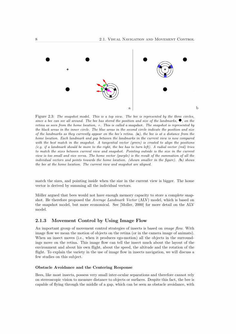
When the bee is displaced from the goal location, the position and size of the landmarkschange. This can be seen in Figure 2.3, where the black areas in the inner circle give theposition and size of the landmarks as taken in the snapshot and the grey areas in the secondcircle give the position and size of the landmarks as they currently appear on the retina. Thewhite areas correspond to the gaps between the landmarks.
A home vector. pointing approximately to the target position, can be derived from pairingeach area in the current view with the closest sector of the same type (landmark or gap) inthe snapshot, where snapshot and current view are aligned in the same compass direction.Each pairing generates two vectors. A tangential vector pointing so as to align the positionof the two areas, from the area in the snapshot to the corresponding area in the current view,because the agent needs to turn in that direction to align the positions. And a radial vector,pointing so as to match the size of the corresponding areas. Pointing outside if the size inthe current view is smaller than in the snapshot, because the agent needs to come closer to
1Although the bee does not have an eye with a single retina, but an compound eye consisting of many’retinae’, we will talk about ’the retina’ in the proceeding chapters of this thesis, for simplicity.
8 2.1. Visual Navigation and Movement Control
a b
Figure 2.3: The snapshot model. This is a top view. The bee is represented by the three circles,since a bee can see all around. The bee has stored the position and size of the landmarks, •, on theretina as seen from the home location, +. This is called a snapshot. The snapshot is represented bythe black areas in the inner circle. The blue areas in the second circle indicate the position and sizeof the landmarks as they currently appear on the bee’s retina. (a), the bee is at a distance from thehome location. Each landmark and gap between the landmarks in the current view is now comparedwith the best match in the snapshot. A tangential vector (green) is created to align the positions(e.g. if a landmark should be more to the right, the bee has to turn left). A radial vector (red) triesto match the sizes between current view and snapshot. Pointing outside is the size in the currentview is too small and vice versa. The home vector (purple) is the result of the summation of all theindividual vectors and points towards the home location. (shown smaller in the figure). (b) showsthe bee at the home location. The current view and snapshot are aligned.
match the sizes, and pointing inside when the size in the current view is bigger. The homevector is derived by summing all the individual vectors.
Moller argued that bees would not have enough memory capacity to store a complete snap-shot. He therefore proposed the Average Landmark Vector (ALV) model, which is based onthe snapshot model, but more economical. See [Moller, 2000] for more detail on the ALVmodel.
2.1.3 Movement Control by Using Image Flow
An important group of movement control strategies of insects is based on image flow. Withimage flow we mean the motion of objects on the retina (or in the camera image of animats).When an insect moves (i.e., when it produces ego-motion) all the objects in the surround-ings move on the retina. This image flow can tell the insect much about the layout of theenvironment and about his own flight, about the speed, the altitude and the rotation of theflight. To explain the variety in the use of image flow in insects navigation, we will discuss afew studies on this subject.
Obstacle Avoidance and the Centering Response
Bees, like most insects, possess very small inter-ocular separations and therefore cannot relyon stereoscopic vision to measure distance to objects or surfaces. Despite this fact, the bee iscapable of flying through the middle of a gap, which can be seen as obstacle avoidance, with

Chapter 2. Insect Navigation 9
Figure 2.4: Illustration of an experiment demonstrating that flying bees infer range from apparentimage speed. The short arrows depict the direction of the flight and the long arrows the direction ofgrating motion. The shaded areas represent the means and standard deviations of the positions ofthe flight trajectories, analysed from video recordings of several hundred flights. From [Srinivasan etal., 1996].
the walls as obstacles. Srinivasan set up a research to see how bees solve this task [Srinivasanet al., 1996]. Figure 2.4 shows the experimental setup of this study. A sugar solution wasplaces at the end of a tunnel. The bees were trained to collect the sugar by flying throughthe tunnel. Each side of the wall carried a pattern consisting of a vertical black-and-whitegrating. The grating on one wall could be moved horizontally to both sides.
When both gratings were kept stationary, the bees flew through the center of the tunnel,i.e., they maintained equidistance to both walls (Fig. 2.4 A). But when one of the gratingswas moved at a constant speed in the direction of the bees flight (thereby reducing the speedof image flow on the eye facing that grating) the bee’s trajectories were shifted to the sideof the moving grating (Fig. 2.4 B). When the grating was moved in the opposite direction(thus increasing the speed of image flow), the trajectories were shifted away from the movinggrating (Fig. 2.4 C). This suggests that the bees keep equidistance to both wall by balancingthe apparent angular speeds of both walls, this is balancing the speed of image flow in botheyes. A lower image speed on one eye was evidently taken to mean that the grating on thatside was farther away and causes the bees to fly closer to that side. Srinivasan even couldmake the bees bump into the wall.
To be sure that the bees balanced the speeds on both sides and not the black-and-whitefrequency of the gratings at both sides. Gratings with different spatial periods were placedon the walls (Fig. 2.4 D,E,F). This did not influence the bees’ flight trajectories, therebyproving that the bees really used the speed of image flow on left and right eye to keep thewalls at equidistance.

10 2.1. Visual Navigation and Movement Control
Regulating Speed
In a similar way Srinivasan et al. [1996] showed that bees regulate the speed of their flightby monitoring the apparent velocity of the surrounding environment. Just as in the previousstudy, the bees were trained to fly through a tunnel, but this time the tunnel was tapered.The flight speed of the bees was exactly so that the apparent speed of the gratings on thewalls maintained constant. The bees slowed down when approaching the narrowest section ofthe tunnel and accelerated when the tunnel widens beyond it. The advantage of this strategyis that the bees automatically slow down when approaching a difficult narrow passage.
Grazing Landing
With exactly the same strategy bees also perform a smooth landing on a horizontal surface[Srinivasan et al., 2000]. When the bee approaches the surface, the apparent speed of thetexture on the surface increases. The bee tries to keep a constant apparent speed and slowsdown. Therefore the speed of the bee is close to zero at touchdown. The advantage ofthis strategy is that control of flight speed is achieved without explicit knowledge about theheight.
Odometry
For a long time the thought was that bees use the amount of energy consumption or thenumber of wingbeats to measure the distance flown (i.e., proprioceptive information). Butsince bees and other arial insects fly and are subject to unknown winds, this strategy seemednot to be a reliable measurement of distance flown for these animals. A headwind, for ex-ample, would then give a bee the impression that it has covered more distance. But howdo bees measure distance flown? The experiments in [Srinivasan, Zhang, and Bidwell, 1997;Srinivasan et al., 2000] showed that bees gain distance traveled by integrating the apparentspeed of the surroundings.
Bees were trained to collect food at the end of a tunnel, which had vertical black-and-whitepatterns at the walls. After a few hours of training, the food source was removed, to test thebee. The next time the bee was to collect the food, it searched for the food in the tunnel.The location with the highest search density was considered to be the place where the beeexpected the food source. When the period of the strips in the tunnel was double or halfthe period during training, the bee expected the food at the correct distance from the tunnelentrance. So the bee did not estimate the distance by counting the number of strips. How-ever, when the bee was tested in a wider tunnel, the bee searched at a greater distance, whileit searched closer to the entrance when the tunnel was narrower. The places where the beeexpected the food source matched the place that one would expect when the bee measureddistance flown by integrating the apparent speed of the black-and-white gratings. Becauseflying through the wider tunnel produced less speed of the stripes, the bee flew further inorder to compensate for this.
These different studies demonstrate the importance of image flow for insect navigation. In-sects use the image flow in different parts of the visual field for different purposes: The lateralparts are used for the centering response, for odometry and for regulating the speed. Fora smooth landing the caudal (under) part is used. This part is also used to regulate of thespeed. For avoiding obstacles which the insect is approaching, the image flow in the frontalpart is used.

Chapter 2. Insect Navigation 11
2.2 Landmark Learning in Bees
When bees, like most insects, want to be able to return to a certain location, they learn theenvironment by the landmarks in the environment. On the point of returning, the landmarkscan pinpoint the goal. However, the bees can use many landmarks. The question is if thebees use all available landmarks for the navigation. If not, which landmarks do bees use andhow do they select these landmarks?
2.2.1 Which Landmarks are Used?
In [Cheng et al., 1987] bees were trained to collect sucrose from a place surrounded by anarray of highly visible cylindrical landmarks. After a few hours of training, the bees weretested singly on a test field containing the array of landmarks (with some modifications), butin the absence of the sucrose. In that case, the bee searched at the position where it expectedthe sucrose. The position of the bee was recorded four times per second.When the bees were trained with two landmarks close to the goal location and two landmarks
TestingTraining
b
a
Figure 2.5: (a) The bees were trained for a few hours to collect sucrose , 2, from a location markedby two near and two distant landmarks, marked by •, both of the same size. In the test, only twolandmarks are placed in the room. The highest search density was at N. This is the location whereone expects the bees to search for the sucrose if they were guided by the landmarks closest to thegoal during training. If the bee would be guided by the two distant landmarks, the highest searchdensity would be at M. (b), the bees were trained with two small landmarks close to the goal andtwo large ones further from the goal. The apparent size of all four landmarks was equal at the goallocation, 2. The bees were tested with two large landmarks placed in the room. If the bees would usthe landmarks with the largest apparent size (all four) they would search both at the left and rightside of the landmarks. But the test showed that the highest search density was at N and not at M.This clearly shows that the bees search at the position as specified by the landmarks closest to thegoal during the training.
further from it, and were tested with only two landmarks, they searched for the food sourceat the position where it should be relative to the two nearby landmarks (see Figure 2.5a).They were not guided by the landmarks further away from the goal. There are two possible

12 2.2. Landmark Learning in Bees
reasons why the nearby landmarks are used to pinpoint the goal. Was that because of thedistance of the landmarks from the goal or because of the apparent size of the landmarks asviewed from the goal location (the nearby landmarks appear bigger on the bees’ retina)? Toexplore this question, the bees were trained with two small landmarks placed near the goaland two bigger landmarks further away from the goal, in such a way that the apparent sizeof all the landmarks was equal at the goal location. During the tests the bees were againguided by the nearby landmarks. The bees did memorize the landmarks further from thegoal, but the nearby landmarks were highly preferable (Figure 2.5b).
In [Collett and Zeil, 1997], it is also concluded that bees are sensitive to the absolute distancetowards objects and that they prefer to be guided by objects near to the goal for detailednavigation. But they added that bees also use distant landmarks for long distance navi-gation. These landmarks have to be large in order for the bee to see them from a greatdistance. Distant landmarks are visible in a large area, but because of the great distance ofthe landmarks and the limited resolution of the bee’s eye, these landmarks can not providein detailed navigation, but they can only guide the bee near the goal area. Landmarks closeto the goal are only visible in a small area and therefore can not be used for navigation overlong distances, but they can much more precisely pinpoint the goal location.
2.2.2 How are the Landmarks Selected?
It is evident that bees are sensitive to the distance of objects, but the question remains: Howdo bees measure the distance towards objects in order to select them for the landmark navi-gation task? As mentioned in section 2.1.2, there are two possible answers to this question:The distance can be gained by using the apparent size of the objects, as was the result in thesnapshot model [Cartwright and Collett, 1983]. The bee can only use this strategy when it hasa priori knowledge about the absolute size of the landmark, for ’bigger is closer’ is not alwaystrue. For example a huge building far from the viewer can appear bigger than a nearby pencil.
The second possible answer is to use the angular velocity of an object when the bee is inego-motion. Everybody who has been in a train noticed at least ones that the poles at thesides of the railway go by the window really quickly, whereas, for instance, a cow far away ina meadow passes much slower. The faster an object seems to move across the retina (i.e., thehigher the angular velocity), the closer the object is. This strategy, that is based on the speedof the image motion, requires a constant speed of the observer during the selection phase,since the speed of the ego-motion also influences the angular velocity of objects. Further morethis strategy requires a stable course. This will be explained in more detail in section 2.3.
Turn-Back and Look behaviour
Lehrer has been studying bees for many years. In one study she looked at the learning phaseof landmark navigation. That is the first few times that the bee visits the home location(e.g. a flower). It is the phase in which the bee learns different cues about the surroundingsat the home location. During one of her experiments she noticed a remarkable behaviourof the bees during the learning phase: The bees performed a so called Turn-Back and Lookbehaviour (TBL) [Lehrer, 1993].
When the bee departs from a flower during the learning phase, it does not fly to the hive in astraight line. The bee flies a short distance away from the flower, then turns around and looksback to the home location, while hovering sideways, to left and right. The bee then continues
Chapter 2. Insect Navigation 13
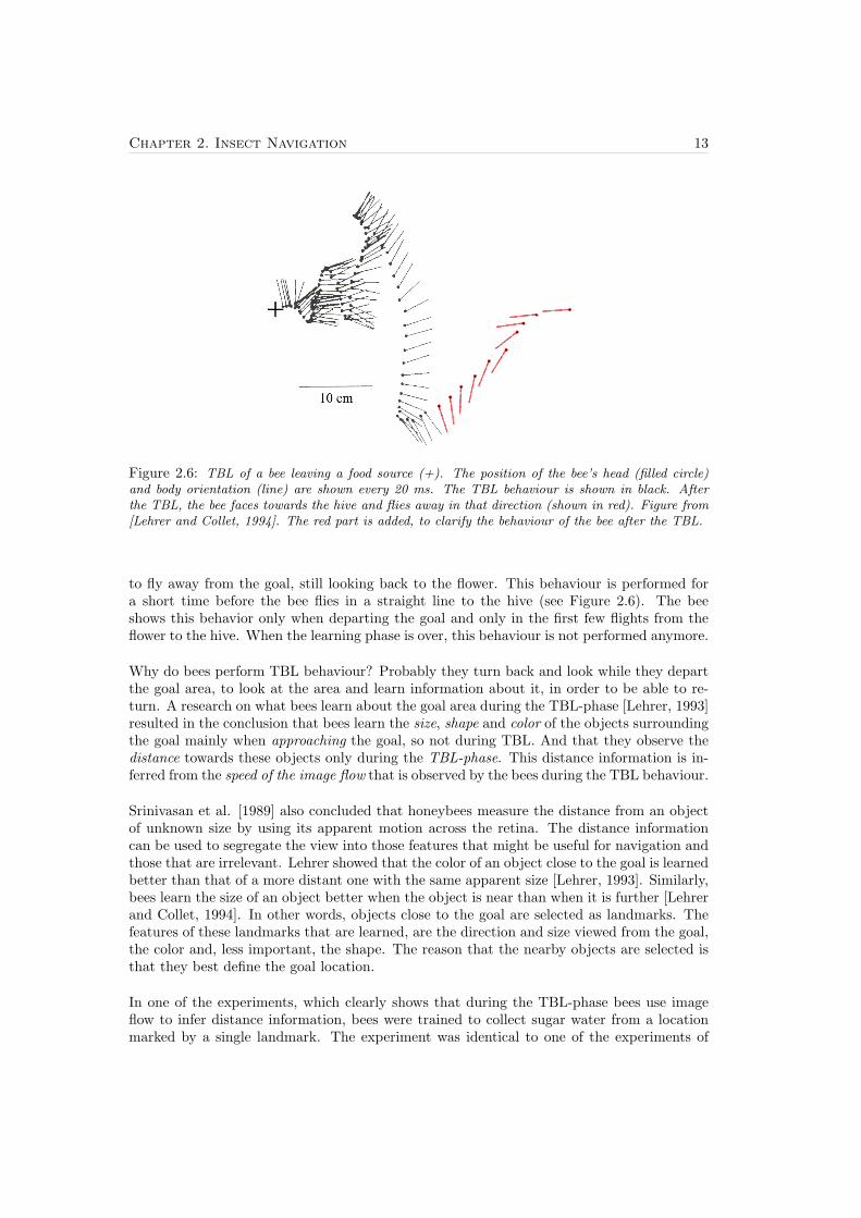
Figure 2.6: TBL of a bee leaving a food source (+). The position of the bee’s head (filled circle)and body orientation (line) are shown every 20 ms. The TBL behaviour is shown in black. Afterthe TBL, the bee faces towards the hive and flies away in that direction (shown in red). Figure from[Lehrer and Collet, 1994]. The red part is added, to clarify the behaviour of the bee after the TBL.
to fly away from the goal, still looking back to the flower. This behaviour is performed fora short time before the bee flies in a straight line to the hive (see Figure 2.6). The beeshows this behavior only when departing the goal and only in the first few flights from theflower to the hive. When the learning phase is over, this behaviour is not performed anymore.
Why do bees perform TBL behaviour? Probably they turn back and look while they departthe goal area, to look at the area and learn information about it, in order to be able to re-turn. A research on what bees learn about the goal area during the TBL-phase [Lehrer, 1993]resulted in the conclusion that bees learn the size, shape and color of the objects surroundingthe goal mainly when approaching the goal, so not during TBL. And that they observe thedistance towards these objects only during the TBL-phase. This distance information is in-ferred from the speed of the image flow that is observed by the bees during the TBL behaviour.
Srinivasan et al. [1989] also concluded that honeybees measure the distance from an objectof unknown size by using its apparent motion across the retina. The distance informationcan be used to segregate the view into those features that might be useful for navigation andthose that are irrelevant. Lehrer showed that the color of an object close to the goal is learnedbetter than that of a more distant one with the same apparent size [Lehrer, 1993]. Similarly,bees learn the size of an object better when the object is near than when it is further [Lehrerand Collet, 1994]. In other words, objects close to the goal are selected as landmarks. Thefeatures of these landmarks that are learned, are the direction and size viewed from the goal,the color and, less important, the shape. The reason that the nearby objects are selected isthat they best define the goal location.
In one of the experiments, which clearly shows that during the TBL-phase bees use imageflow to infer distance information, bees were trained to collect sugar water from a locationmarked by a single landmark. The experiment was identical to one of the experiments of

14 2.2. Landmark Learning in Bees
Training TestingTraining Testing
Experienced beesLearining bees
a b
Figure 2.7: In both experiments, the bees were trained to collect sugar water from a location, 2,marked by a single landmark, •. In experiment (a), the bees were trained only for a few trials, so thatthey were still in the learning phase. When the bees were tested in a test field with a bigger landmarkand in the absence of the sugar water, they searched at the location with the same orientation anddistance towards the landmark, N. At a distance where the landmark produced the same amount ofimage flow as during training. Experiment (b), is an identical experiment, but now the bees weretrained for half a day and so were experienced. The bees now searched at a location with the sameorientation, but with a larger distance towards the landmark, N. At a distance where the landmarkappeared at the same size as during training.
Cartwright and Collett, except that this time the bees were not trained for many hours, butjust for a few flights. During the test, a bigger landmark was placed in the test field. Thistime the bees searched for the food source at the correct distance from the landmark, wherethe image flow of the landmark was equal to that during training, although the apparent sizeof the landmark was much bigger (see Figure 2.7).
So we see two distinct phases, the learning phase and the phase when the learning phase isover, the landmark navigation phase. During the learning phase, when the landmarks areselected and learned, bees use image flow to gain a 3-D perspective of the world by performingTBL. During the landmark navigation phase, when the sizes of the landmarks are alreadylearned, the bees use the apparent size of the object to measure the distance. The reasonfor this shift in the bee’s behaviour is that the use of image flow for the absolute distance ismore cumbersome than relying on the apparent size, because on each approach the returningbee would need to scan the scene as it did during the TBL phase.
2.2.3 Which Landmark Cues are Learnt?
Which information about the landmarks does the bee learn? From [Cartwright and Collett,1983] we know that the bee remember the apparent size and the position on the retina as viewfrom the home location. By using the apparent motion of objects the bee gains informationabout the distance [Lehrer, 1993; Srinivasan et al., 1989]. Lehrer tells us that the bee alsoremembers the color of the landmarks [Lehrer, 1993]. And at last we know that bees learnthe shape of the landmarks [Lehrer, 1993; Hateren, Srinivasan, and Wait, 1990].
Chapter 2. Insect Navigation 15
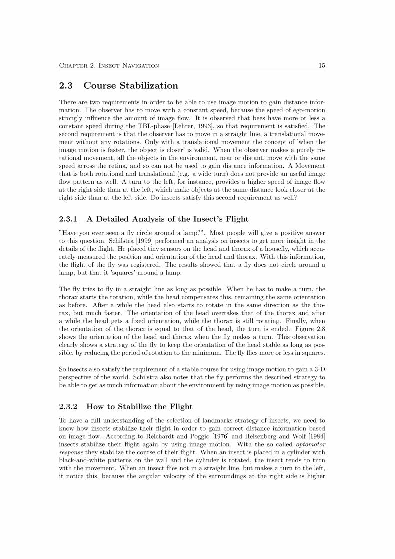
2.3 Course Stabilization
There are two requirements in order to be able to use image motion to gain distance infor-mation. The observer has to move with a constant speed, because the speed of ego-motionstrongly influence the amount of image flow. It is observed that bees have more or less aconstant speed during the TBL-phase [Lehrer, 1993], so that requirement is satisfied. Thesecond requirement is that the observer has to move in a straight line, a translational move-ment without any rotations. Only with a translational movement the concept of ’when theimage motion is faster, the object is closer’ is valid. When the observer makes a purely ro-tational movement, all the objects in the environment, near or distant, move with the samespeed across the retina, and so can not be used to gain distance information. A Movementthat is both rotational and translational (e.g. a wide turn) does not provide an useful imageflow pattern as well. A turn to the left, for instance, provides a higher speed of image flowat the right side than at the left, which make objects at the same distance look closer at theright side than at the left side. Do insects satisfy this second requirement as well?
2.3.1 A Detailed Analysis of the Insect’s Flight
”Have you ever seen a fly circle around a lamp?”. Most people will give a positive answerto this question. Schilstra [1999] performed an analysis on insects to get more insight in thedetails of the flight. He placed tiny sensors on the head and thorax of a housefly, which accu-rately measured the position and orientation of the head and thorax. With this information,the flight of the fly was registered. The results showed that a fly does not circle around alamp, but that it ’squares’ around a lamp.
The fly tries to fly in a straight line as long as possible. When he has to make a turn, thethorax starts the rotation, while the head compensates this, remaining the same orientationas before. After a while the head also starts to rotate in the same direction as the tho-rax, but much faster. The orientation of the head overtakes that of the thorax and aftera while the head gets a fixed orientation, while the thorax is still rotating. Finally, whenthe orientation of the thorax is equal to that of the head, the turn is ended. Figure 2.8shows the orientation of the head and thorax when the fly makes a turn. This observationclearly shows a strategy of the fly to keep the orientation of the head stable as long as pos-sible, by reducing the period of rotation to the minimum. The fly flies more or less in squares.
So insects also satisfy the requirement of a stable course for using image motion to gain a 3-Dperspective of the world. Schilstra also notes that the fly performs the described strategy tobe able to get as much information about the environment by using image motion as possible.
2.3.2 How to Stabilize the Flight
To have a full understanding of the selection of landmarks strategy of insects, we need toknow how insects stabilize their flight in order to gain correct distance information basedon image flow. According to Reichardt and Poggio [1976] and Heisenberg and Wolf [1984]insects stabilize their flight again by using image motion. With the so called optomotorresponse they stabilize the course of their flight. When an insect is placed in a cylinder withblack-and-white patterns on the wall and the cylinder is rotated, the insect tends to turnwith the movement. When an insect flies not in a straight line, but makes a turn to the left,it notice this, because the angular velocity of the surroundings at the right side is higher

16 2.4. Conclusion
Figure 2.8: The orientation of the thorax (blue dashed line, t) and the head (red line, h) duringa turn. During the turn, the thorax makes a roll, the head almost completely compensates for this.The head also compensates thorax rotation around the vertical axis (yaw, both at the beginning andat the end of the turn, in the middle of the turn, the yaw of the head is faster than that of thethorax. The result is that the period of rotational movement is reduced, thereby increasing the periodof translational movement. Thus increasing the period in which the insect gains depth information.Figure from [Schilstra, 1999].
than that at the left side. Subsequently, the insect compensates for this by turning to theright in order to stabilize the flight.
2.4 Conclusion
We can conclude that bees use vision, especially image flow, for many navigation and move-ment control strategies. Landmark navigation is an important visual navigation strategy.Bees use landmarks to guide them to a goal. Bees do not use all available objects in thesurroundings. During the learning phase, they select objects near the goal as landmarks.These nearby objects are selected by using image motion. The device is: The higher theangular velocity of an object, the closer the object is. The preconditions to obtain distanceinformation from image flow are that the bees maintain a constant speed and a stable flight.Bees stabilize their flight again by using image flow.

Chapter 2. Insect Navigation 17
In the next chapter, we will use the biological findings about the landmark selection topropose a model for landmark selection in an autonomous flying robot. The model consistsof two submodels. The flight-stabilization model and the actual landmark-selection model.Both models are based on the biological studies that we outlined in section 2.2 and 2.3.


Chapter 3
A Visual Landmark-SelectionModel for Flying Robots
Figure 3.1: Melissa, the flying robot platform
3.1 Melissa
The models we will propose in this chapter, will all be implemented on a flying robot platformcalled Melissa (see Figure 3.1). Melissa is a blimp-like flying robot, consisting of a heliumballoon, a gondola hosting the on-board electronics, and a off-board host computer. Theballoon is 2.3m long and has a lift capacity of approximately 400g. The gondola hosts theelectronics for the perception and action of the robot.
3.1.1 Perception
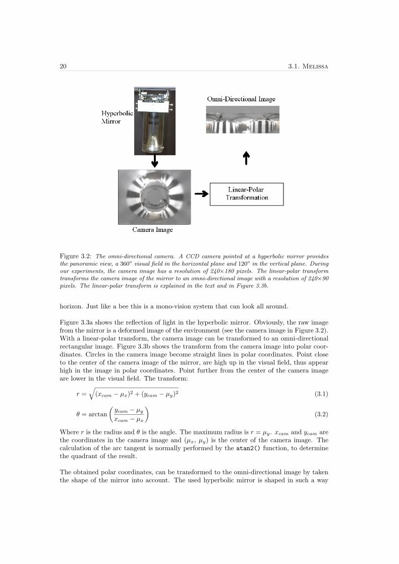
Insects use their vision to select landmarks. Therefore we equip Melissa with an omni-directional vision system, which provides the sensory input (see Figure 3.2).
The omni-directional vision system consists of a CCD-camera placed in front of a hyperbolicmirror, based on a panoramic optics studie [Chahl and Srinivasan, 1997]. This provides a360o panoramic visual field in the horizontal plane and 120o in the vertical plane, around the
19
20 3.1. Melissa
Figure 3.2: The omni-directional camera. A CCD camera pointed at a hyperbolic mirror providesthe panoramic view, a 360o visual field in the horizontal plane and 120o in the vertical plane. Duringour experiments, the camera image has a resolution of 240×180 pixels. The linear-polar transformtransforms the camera image of the mirror to an omni-directional image with a resolution of 240×90pixels. The linear-polar transform is explained in the text and in Figure 3.3b.
horizon. Just like a bee this is a mono-vision system that can look all around.
Figure 3.3a shows the reflection of light in the hyperbolic mirror. Obviously, the raw imagefrom the mirror is a deformed image of the environment (see the camera image in Figure 3.2).With a linear-polar transform, the camera image can be transformed to an omni-directionalrectangular image. Figure 3.3b shows the transform from the camera image into polar coor-dinates. Circles in the camera image become straight lines in polar coordinates. Point closeto the center of the camera image of the mirror, are high up in the visual field, thus appearhigh in the image in polar coordinates. Point further from the center of the camera imageare lower in the visual field. The transform:
r =√
(xcam − µx)2 + (ycam − µy)2 (3.1)
θ = arctan(ycam − µyxcam − µx
)(3.2)
Where r is the radius and θ is the angle. The maximum radius is r = µy. xcam and ycam arethe coordinates in the camera image and (µx, µy) is the center of the camera image. Thecalculation of the arc tangent is normally performed by the atan2() function, to determinethe quadrant of the result.
The obtained polar coordinates, can be transformed to the omni-directional image by takenthe shape of the mirror into account. The used hyperbolic mirror is shaped in such a way

Chapter 3. A Visual Landmark-Selection Model for Flying Robots 21
r1 θ1
θ1
µ x (w ,h )c c 2π xµ( , ) (w , )c µy
b
θ x
yr
µ y(0,0) (0,0)
Camera Image Polar Coordinates Omni−Directional Image
(0,0)
cam
xcam
y
r1
a
hyperbolicmirror
camera
Figure 3.3: (a) shows the reflection of light in the hyperbolic mirror. The mirror is shaped in such away that each pixel spans the same angle in the visual field. (b) shows the transform from the cameraimage of the mirror to the omni-directional image. A polar transform is used to transform the imageinto polar coordinates and linear transform transforms the polar coordinates to the omni-directionalimage. xcam and ycam are the coordinates in the camera image, θ and r are the polar coordinatesand x and y are the coordinates in the omni-directional image. A circle close to the center of thecamera image (µx,µy) is a straight line in the omni-directional image, high up in the visual field(blue). A circle further from the center (red) corresponds to a line lower in the visual field.
that it is equi-angular. This implicates that each pixel in the camera image spans the sameangle of view, irrespective of its distance from the center of the image. (See [Chahl andSrinivasan, 1997] for more detail). The consequence of the equi-angular property of themirror is that the omni-directional image can be obtained by performing a linear transformof the polar-coordinates.(
xy
)=(
wc2π1
)·(θr
)(3.3)
Where x and y are the coordinates in the omni-directional image and wc is the width of thecamera image (wc = 2µx). The resolution of the original camera image is wc×hc. Due to thetransformations (3.1), (3.2) and (3.3), the resolution of the omni-directional image is wc×µy.
During our experiment we used a resolution of the camera image of 240×180 pixels. Thisgives an omni-directional image with a resolution of 240×90 pixels.
3.1.2 Action
The flying robot can act in three dimensional space. By means of three motors, the robotcan translate back and forward, rotate to the left and the right and translate up and down.

22 3.2. The Elementary Motion Detector
There are two propellers at the left and right side of the gondola. Both run at the samevariable speed either clockwise or counterclockwise and both are attached to the same spindle,which can change the orientation of the propellers, so that the robot can go up-down andback-forward (see Figure 3.4 A). The rotation of the robot to the left and the right is providedby a single propeller at the tail of the blimp.
a b
Figure 3.4: (a)The gondola under the blimp. The two propellers are attached to one spindle, whichcan change the orientation. In this way, the robot can move up-down and back-forward. At the tailof the robot (not shown) is a single propeller, which can let the robot rotate left and right. (b) showsthe sensory-motor loop. The robot sends the images to the host computer. The host computer sendsappropriate action commands to the robot, which acts accordingly. This action will make a changein the perception of the robot.
3.1.3 The Sensory-Motor Loop
The video signal of the camera is sent by wireless transmission to a receiver which is attachedto a frame grabber on the host computer, with a maximum frame rate of 25 Hz. At the hostcomputer the processing of the camera image is done and the appropriate action is deter-mined. Three bytes are sent to a digital/analog converter(DAC), one for each movement(i.e., back-forward(BF), rotating left-right(LR) and up-down(UD)). The bytes have valuesbetween 0-255. Thereupon, the bytes are converted to voltages between 2-4 Volts and placedon separate channels, which are sent to the radio transmitter. The radio transmitter convertsthe electric signals to radio signals on different frequencies and sends those to the blimp. Theradio signals are received in the blimp, where the different channels BF, LR and UD are in-terpreted and the actions are performed by the motors. (See Figure 3.4 B.)
During our experiments (see section 4), we obtained a frame rate of 10 Hz. Every second, 10sensory-motor loops were completed in the algorithm.
3.2 The Elementary Motion Detector
As we discussed in chapter 2, the problem of selecting nearby landmarks based on the appar-ent speed of the objects in the visual field, consists of two systems: Stabilizing the flight anddetecting the angular velocity of objects. In nature, both systems rely on a system that candetect motion in the visual field. This means that in order to make a model for the selection
Chapter 3. A Visual Landmark-Selection Model for Flying Robots 23
of nearby landmarks, we need a model for detecting motion in the visual field, a so calledmotion detector.
In past research, many motion detectors were proposed, some of them from a statistical ormathematical point of view , and others were a result of biological studies (see [Barron, Fleet,and Beauchemin, 1994] for an overview of motion detectors). There exist good models withinboth approaches, but since we are working in the framework of biorobotics, we are interestedin the biologically plausible models for detecting motion only.
One of the most well known biologically plausible motion detection models is the ElementaryMotion Detector (EMD), initially proposed by Reichardt [1969]. He performed a series ofbehavioral studies on the optomotor response of insects, that is, their evoked response tomovements relative to themselves in their visual surroundings. He performed these studies tofind some fundamental functional principles of the insect central-nervous system, responsiblefor the optomotor response. Guided by these principles, Reichardt proposed his minimalmodel for optomotor movement perception, the EMD model. For our model we used theEMD model with some small modifications, as proposed in [Borst and Egelhaaf, 1993], whichwe will discuss in the next section.
3.2.1 General EMD Model
+ −
Photoreceptor
High−pass filter
Low−pass filter
Multiplication
Subtraction
Pixels
Intensity value∆ϕ
Movementof edge
EMD Output
λ λ1 2
1
left
1
right
O
MM
L L 2
H2H
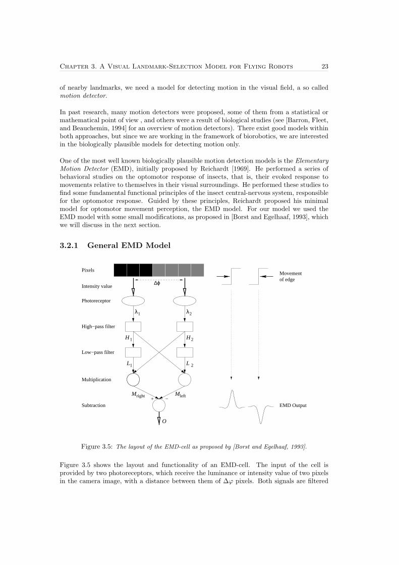
Figure 3.5: The layout of the EMD-cell as proposed by [Borst and Egelhaaf, 1993].
Figure 3.5 shows the layout and functionality of an EMD-cell. The input of the cell isprovided by two photoreceptors, which receive the luminance or intensity value of two pixelsin the camera image, with a distance between them of ∆ϕ pixels. Both signals are filtered

24 3.2. The Elementary Motion Detector
by a first-order difference ’high-pass’ filter:
Hi[t] = λi[t]− λi[t− 1] (3.4)
Where λi is the luminance (or intensity) as measured by photoreceptor i and Hi is the outputsignal of high-pass filter i. This means that the output of the high-pass filter is equal to thechange in intensity from time t− 1 to time t.The output of both high-pass filters are then low-pass filtered by a first-order recursive ’low-pass’ filter:
Li[t] = α ·Hi[t] + (1− α) · Li[t− 1] (3.5)
Where LPHi is the output signal of low-pass filter i and α is the discrete RC-filter coefficient.This is a recursive exponential filter, because an input signal of the filter decays exponentiallyover time. Due to this decaying property and the fact that the high-pass filter only gives anon-zero output if there is a change in the luminance, the output value of the exponentialfilter tells us something about how long ago there was a luminance event. The lower theoutput value of the low-pass filter, the longer ago a luminance event took place. α is thetime coefficient of the filter. When α → 0 the decay is slow and the signal over a long timeis considered, when α → 1, the decay is fast and the signal is only considered over a shortperiod of time.
In the next processing stage, the output of the low-pass filter at one side is multiplied withthe output of the high-pass filter at the other side of the EMD-cell.
Mright[t] = L1[t] ·H2[t] (3.6)Mleft[t] = L2[t] ·H1[t] (3.7)
Where Mright is the output signal of the multiplication, which is sensitive for motion fromleft to right. Mleft is sensitive for motion from right to left.
When an object moves from left to right and the first edge of the object reaches the leftphotoreceptor, there is a change in luminance λ1. This results in a non-zero signal H1, whichcomes into the first low-pass filter, resulting in a decaying output signal L2. Since there hasnot been a change in luminance λ2, the output H2 is still zero, so the output of the multi-plication Mright is zero. For a certain period of time both high-pass filters give zero output.When the edge of the object reaches the right photoreceptor of the cell, a luminance eventtakes place at lambda2, which gives a non-zero output of the high-pass filter H2. Becausethere is still an output signal of the low-pass filter, L1, the output of the multiplication,Mright, is non-zero, whereas output Mleft is still zero. When the second edge of the objectpasses the EMD-cell, again there is a pulse in the signal Mright and signal MP2 stays zero.Because the EMD-cell is symmetrical it is obvious that the signal Mleft is sensitive for motionfrom right to left.
The EMD-cell is also called a correlation model, because it correlates an edge at one pho-toreceptor at a certain time with the same edge at the other receptor later in time.
The final step in the EMD-cell is the subtraction of the signal given by the multipliers, tomake the cell sensitive to both leftward and rightward movements.
O = Mright −Mleft (3.8)

Chapter 3. A Visual Landmark-Selection Model for Flying Robots 25
Where O is the effective output signal of the EMD-cell after the subtraction. If there is mo-tion to the left, Mleft > Mright, which results in a negative output signal O. Movement to theright gives a positive output. Besides that the cell is sensitive to the direction of the motion,it is also sensitive to the motion’s velocity. When the velocity is high, the time between theactivation of the first photoreceptor and the second is small. Therefore the low-pass filtergives a high output signal, which results in a high output signal of the EMD-cell, O. Whereaswith a slower movement, the signal of the low-pass filter is more decayed, which results in alower EMD output.
There are two parameters in this model that can tune the sensitivity of the EMD-cell; thetime coefficient of the low-pass filter, α, and the distance measured in pixels between the twophotoreceptors, ∆ϕ. With α→ 0, the cell is sensitive to slow motion. Whereas with α→ 1,the decay factor of the low-pass filter is fast, consequently the cell is sensitive to fast motion.Since we are working with a camera input which is not continuous but works with discreteimages (i.e., frames), the EMD output is also calculated in a discrete manner. This meansthat the maximum velocity which can be detected by the cell is ∆ϕ pixels/frame. A fastermotion will simply pass both photoreceptors in between two successive frames and thereforewill not activate the EMD cell. So a small value for ∆ϕ will make the cell sensitive to slowmotions and a bigger value makes the cell sensitive to faster motions.
There are some other considerations when tuning these two parameters: A slow decay of thelow-pass filter (small value for α) has the drawback that it might result in a wrong correlation,a correlation between two different edges. Because the signal decays so slow, the low-passfilter might still give a signal even when a moving edge has already been detected. Whena second edge passes the EMD-cell, the previous edge might interfere with the correlationof the new edge. A similar drawback occurs when the distance between the photoreceptors,∆ϕ, is to large. In that case, one edge might activate the first photoreceptor, while anotheredge activates the second photoreceptor. This also results in a wrong correlation betweentwo different edges. So α and ∆ϕ need to be tuned in such a way that the cell is sensitive tothe desired motion velocities and that it is least bothered with the drawbacks.
When we use this EMD-cell as a motion detector, the output signal of the cell tells us thedirection of the motion and gives a good indication about the velocity of the motion in theimage.
3.2.2 EMD3 Model
Although the EMD model, as described in the previous section, is very well-known and widelyused, there are some drawbacks: The model is not only sensitive to the direction and velocityof the motion, but also to the spatial structure of the moving object, to the intensity valuesand the spatial frequency [Zanker, Srinivasan, and Egelhaaf, 1999]. Since we want to usethe model to detect the direction and velocity of objects moving in the image, this is notdesirable. We will first have a look at the problems.
Sensitivity to the Intensity Values
The output of the EMD-cell depends on the intensity values. Imagine a red object moving ona black background. Black gives λi = 0.0 and the luminance of red λi = 0.33. If the objectpasses the cell, the high-pass filters give an output value of 0.33, which results in a certain
26 3.2. The Elementary Motion Detector
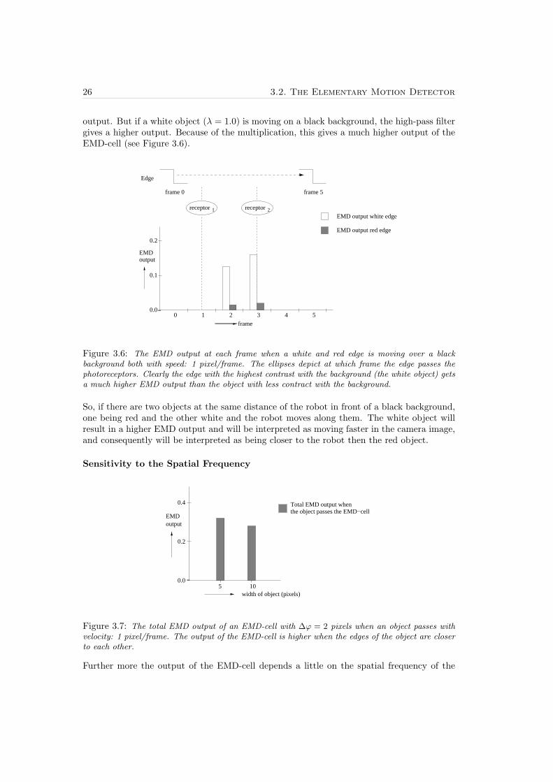
output. But if a white object (λ = 1.0) is moving on a black background, the high-pass filtergives a higher output. Because of the multiplication, this gives a much higher output of theEMD-cell (see Figure 3.6).
0.2
0.1
0 1 2 3 40.0
frame 5
Edge
EMD output white edge
EMD output red edge
frame
EMDoutput
frame 0
5
receptor 1 receptor 2
Figure 3.6: The EMD output at each frame when a white and red edge is moving over a blackbackground both with speed: 1 pixel/frame. The ellipses depict at which frame the edge passes thephotoreceptors. Clearly the edge with the highest contrast with the background (the white object) getsa much higher EMD output than the object with less contract with the background.
So, if there are two objects at the same distance of the robot in front of a black background,one being red and the other white and the robot moves along them. The white object willresult in a higher EMD output and will be interpreted as moving faster in the camera image,and consequently will be interpreted as being closer to the robot then the red object.
Sensitivity to the Spatial Frequency
0.0
EMDoutput
105width of object (pixels)
0.4
0.2
Total EMD output whenthe object passes the EMD−cell
Figure 3.7: The total EMD output of an EMD-cell with ∆ϕ = 2 pixels when an object passes withvelocity: 1 pixel/frame. The output of the EMD-cell is higher when the edges of the object are closerto each other.
Further more the output of the EMD-cell depends a little on the spatial frequency of the
Chapter 3. A Visual Landmark-Selection Model for Flying Robots 27
moving object. The smaller the distance between two successive edges, the higher the EMDoutput (see Figure 3.7. The reason for this is the recursive property of the low-pass filter.When the first edge passes the first photoreceptor of the EMD-cell, the low-pass filter givesa output that slowly decays. When the first edge passes the second receptor, the EMD-cellgives an output, based on the output value of the low-pass filter. But the filter is then notreseted, but there remains a (still decaying) value. When the second edge passes the firstreceptor, we see, if we take a look at (3.5), that the old output of the low-pass filter is addedto the new output of the high-pass filter, which gives a higher new output of the low-passfilter and so a higher output of the EMD-cell. If the two edges are closer to each other, theremaining output value of the low-pass filter is higher, so the output of the EMD-cell is higher.
Solution
We did not solve the last problem of the EMD being sensitive to the spatial frequency ofthe moving object. A solution to the problem could be to reset the low-pass filter after thematching of an edge between the first and second photoreceptor. Adding this functionalityto the EMD-cell would spoil a lot of it’s beauty of simplicity. Further more this problemhas got a minor impact on the EMD output as we can see from Figure 3.7. So solving theproblem is not really necessary.
However, the problem of the EMD being sensitive to the intensity values has got a muchbigger impact. This strongly influences the output of the EMD. Different color intensitiesresult in a great difference in the magnitude of the EMD output. To solve this problem, wehad to see to it that the high-pass filters give a constant output whenever there is a changein the luminance as sensed by the photoreceptors.
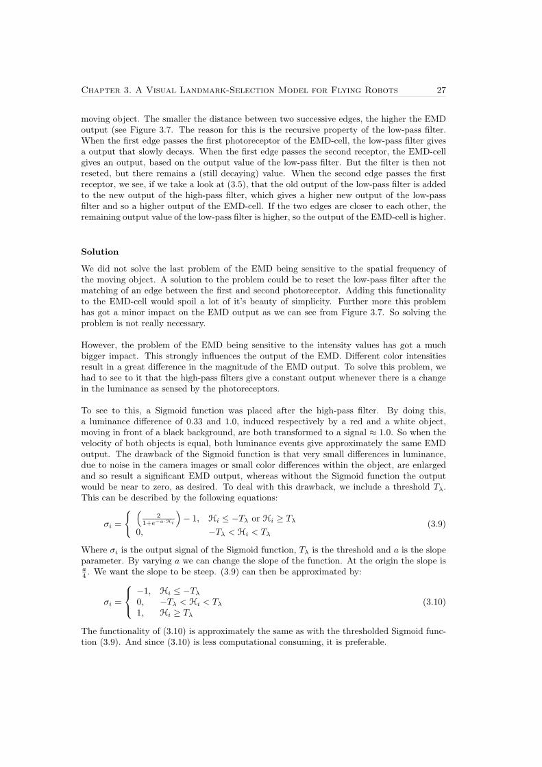
To see to this, a Sigmoid function was placed after the high-pass filter. By doing this,a luminance difference of 0.33 and 1.0, induced respectively by a red and a white object,moving in front of a black background, are both transformed to a signal ≈ 1.0. So when thevelocity of both objects is equal, both luminance events give approximately the same EMDoutput. The drawback of the Sigmoid function is that very small differences in luminance,due to noise in the camera images or small color differences within the object, are enlargedand so result a significant EMD output, whereas without the Sigmoid function the outputwould be near to zero, as desired. To deal with this drawback, we include a threshold Tλ.This can be described by the following equations:
σi =
{ (2
1+e−a·Hi
)− 1, Hi ≤ −Tλ or Hi ≥ Tλ
0, −Tλ < Hi < Tλ(3.9)
Where σi is the output signal of the Sigmoid function, Tλ is the threshold and a is the slopeparameter. By varying a we can change the slope of the function. At the origin the slope isa4 . We want the slope to be steep. (3.9) can then be approximated by:
σi =
−1, Hi ≤ −Tλ0, −Tλ < Hi < Tλ1, Hi ≥ Tλ
(3.10)
The functionality of (3.10) is approximately the same as with the thresholded Sigmoid func-tion (3.9). And since (3.10) is less computational consuming, it is preferable.

28 3.2. The Elementary Motion Detector
x x xx
1
1
1 2
2
1
rightright1
2
MAX right MAX left
32
Photoreceptor
High−pass filter
ThresholdedSigmoid
Low−pass filter
Multiplication
MAX−operator
Subtraction
∆ϕ1 ∆ϕ2
H H H3
LL
L32
MM
O
2leftM1leftM
σσ 3σ
λλλ
Figure 3.8: The 3EMD model. In addition to the general EMD model, there is a Sigmoid functionafter the high-pass filter, which provides a constant output whenever there is a change in luminanceλ. And the cell has an extra photoreceptor which allows the cell to be sensitive for slower motions(v = ∆ϕ1 pix/frame) as well as for faster motions (v = ∆ϕ2 pix/frame). The MAX operator decideswhich branch makes the best match. When the widest branch ’wins’, the output signal of the multipliergets multiplied by 2, because the distance between the photoreceptors is twice as much as in the caseof the shortest branch. This is the model that is used during our research.
Figure 3.8 shows that there is another modification to the general EMD-cell. There a thirdphotoreceptor. The reason for this is that the distance between the photoreceptors, ∆ϕ,partly determines to which velocity the EMD-cell is most sensitive. We want the cell to besensitive to faster motions (v ≈ ∆ϕ1pix/frame) but consequently the cell is than less accuratewith slower motions. To add a third ’branch’, both the faster (v = ∆ϕ2pix/frame) and theslower motion (v = ∆ϕ1pix/frame) can be captured.
With this third branch the multiplications become:
Mright1[t] = L1[t] · σ3[t] (3.11)Mright2[t] = L2[t] · σ3[t] (3.12)Mleft1[t] = L2[t] · σ1[t] (3.13)Mleft2[t] = L3[t] · σ1[t] (3.14)
Where Mright∗ are the output signals of the multipliers which are sensitive to motion from

Chapter 3. A Visual Landmark-Selection Model for Flying Robots 29
left to right and the Mright∗ signals are sensitive to motion to the left. This EMD layoutalso demands a decision maker to decide which branch, the wider or the shorter, makes thebest match. This decision maker is the MAX-operator which is placed after the multipliers.The branch that has the highest multiplier output signal ’wins’ and that signal is passed on.If this is the signal of the wider branch, the signal is multiplied by 2, because the distancebetween both photoreceptors is twice that of the shorter branch. The MAX operators:
MAXright ={
2 ·Mright1 , Mright1 ≥Mright2
Mright2 , Mright1 < Mright2
MAXleft ={
2 ·Mleft2 , Mleft2 ≥Mleft1
Mleft1 , Mleft2 < Mleft1
(3.15)
Where MAXright is the output of the MAX-operator that is sensitive to motion to the rightand MAXleft to the left. Finally the EMD output is obtained by:
O = MAXright −MAXleft (3.16)
Parameters
We need to establish a few parameters in order to use the EMD3 model. First of all we needto set the spatial distances in pixels between the photoreceptors (i.e., ∆ϕ1 and ∆ϕ2). Themaximal detectable angular velocity depends on ∆ϕ2, for:
0.04mind
α
β
0.02
Figure 3.9:
ωmax = ∆ϕ2 pixels/frame (3.17)
A few facts about the robot:
Frame rate of camera: f = 10 HzSpeed of robot: vr = 0.4 m/sResolution of image: ρ = 240/2π pixels/rad
ωmax depends on the frame rate of the camera, speed of the robot, resolution of the imageand on the minimum distance of an object. The first three variables are facts we have to deal

30 3.2. The Elementary Motion Detector
with (see above table). We only have to choose the minimum distance of an object at whichit is detectable. An object at a distance closer than that minimum has an angular velocitywhich is to fast to detect. We choose this minimum:
Minimum distance of object: dmin = 0.5 m
Now we can determine the maximal angular velocity that should be detectable. Figure 3.17show the situation when the robot passes an object during an interval of 1 frame. Thedisplacement of the robot in that interval is:
x = vr/f = 0.04 m (3.18)
The object is at distance dmin. We want to know ∠β in order to get ωmax
α = arctan(12x
dmin) (3.19)
β = 2α = 2 · arctan(x
2dmin) = 8.0 · 10−2rad (3.20)
β is the change in angle over a period of 1 frame, so we can say that the angular velocity ofthe object 8.0 · 10−2 rad/frame. Since dmin is the minimum distance of an object and sincethe robot passes the object, this is the maximum angular velocity of an object. So:
ωmax = β = 8.0 · 10−2 rad/frame (3.21)
The camera image is 240 pixels wide and covers 2π rad. This gives a resolution, ρ, of 240/2πpixels/rad. So,
ωmax = β · ρ = 3.1 pixels/frame (3.22)
If we now look at (3.17), we see:
∆ϕ2 = β · ρ = 3.1 pixels (3.23)
Since ∆ϕ2 has to be an integer, we take the smallest integer > 3.1. Because the EMD3 modelneeds to be symmetrical, ∆ϕ1 is simply the half of this value:
∆ϕ1 = 2 pixels∆ϕ2 = 4 pixels
Then we have to establish the time coefficient of the low-pass filter, α in (3.5). The valueof this parameter can not be calculated, but has to arise from observations of the model inreal-world environments. α = 0.20 gave the best results. With higher values the decay ofthe filter was to fast to detect slower motions. With lower values the problem of a wrongcorrelation between two different edges, as discussed earlier, came about:
α = 0.20
The last parameter that has to be established is the threshold in the Sigmoid function, (3.10).This parameter defines how big the difference of luminance should be to mark it as an edge.Again this value is established by observations in the real world. Tλ = 0.10 turned out to bethe most usable. With a lower value, small differences in luminance within one object werewrongly marked as edges. Whereas with a higher value, many edges in the environment werenot detected:
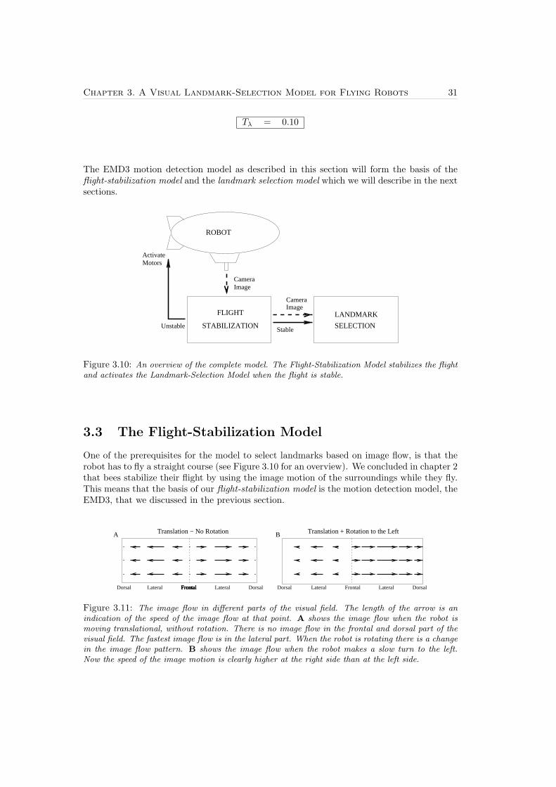
Chapter 3. A Visual Landmark-Selection Model for Flying Robots 31
Tλ = 0.10
The EMD3 motion detection model as described in this section will form the basis of theflight-stabilization model and the landmark selection model which we will describe in the nextsections.
ROBOT
LANDMARK
SELECTION
CameraImage
ActivateMotors
Unstable Stable
CameraImage
STABILIZATION
FLIGHT
Figure 3.10: An overview of the complete model. The Flight-Stabilization Model stabilizes the flightand activates the Landmark-Selection Model when the flight is stable.
3.3 The Flight-Stabilization Model
One of the prerequisites for the model to select landmarks based on image flow, is that therobot has to fly a straight course (see Figure 3.10 for an overview). We concluded in chapter 2that bees stabilize their flight by using the image motion of the surroundings while they fly.This means that the basis of our flight-stabilization model is the motion detection model, theEMD3, that we discussed in the previous section.
Translation − No Rotation
FrontalFrontalFrontalLateralDorsal Lateral DorsalFrontal Dorsal FrontalLateral Lateral Dorsal
A Translation + Rotation to the LeftB
Figure 3.11: The image flow in different parts of the visual field. The length of the arrow is anindication of the speed of the image flow at that point. A shows the image flow when the robot ismoving translational, without rotation. There is no image flow in the frontal and dorsal part of thevisual field. The fastest image flow is in the lateral part. When the robot is rotating there is a changein the image flow pattern. B shows the image flow when the robot makes a slow turn to the left.Now the speed of the image motion is clearly higher at the right side than at the left side.

32 3.3. The Flight-Stabilization Model
The task of the flight-stabilization model is to let the robot fly in one straight line. This meansthat the model has to see to it that there is no rotation and no elevation of the robot. Wedo that by using image flow information while moving through the environment. Basicallythe model tries to equalize the average speed of image motion on the left and right side tostabilize the rotation and on the upper and lower side to stabilize the elevation. If the robotis rotation to the left, the average speed of the image motion is more on the right side thanon the left side (see Figure 3.11). The robot than has to turn to the right, to neutralize theleftward rotation. If the robot flies without rotation, the average speed on the left and rightside of the robot are equal.
For the stabilization of the rotation we only use the frontal and dorsal (back) part of the visualfield. In these the parts there is hardly any image motion when the robot flies straight. Whenthe robot rotates there obviously is a change in the image motion in these parts. Anotherreason to not use the lateral parts is the following: When the robot flies straight, but close toan object at the left side and far from an object on the right side, the speed of image motionin the left lateral part of the visual field is much higher then at the right lateral part. If wewould have used the lateral part to stabilize the course of the robot, the consequence wouldbe that the robot senses a rotation to the right. The frontal and dorsal part are not ’fooled’by the difference between the distance towards objects on the left and right side and so arebetter used for the stabilization of the robot.
Rotation Motor
N A A Nl l r r
y
Division
Low−pass filter
SituationDistinguish
ArlA
totA
Frontal DorsalDorsal
EMD Left EMD Right60−60−120o o o o120
Figure 3.12: The Flight-Stabilization Model. In this figure, only the model for stabilization of therotation is shown. The model for stabilization of the elevation is not shown, but is similar. An arrayof EMD3-cells is placed in the frontal and dorsal part of the visual field on both the left and rightside. The cells are horizontally oriented. The output of the active cells on both sides are summoned(Al and Ar) and the average EMD output of the active cells is taken (Al and Ar). The rotation ofthe robot is analysed by looking at Atot
Figure 3.12 shows the layout of the stabilization model that we propose. It show only thestabilization of the rotation. This is for simplicity. The stabilization of the elevation is simi-

Chapter 3. A Visual Landmark-Selection Model for Flying Robots 33
lar, with the only difference that the orientation of the EMD3-cells is different. For rotationstabilization, the cells are oriented horizontally, which means that the three inputs of the cellare obtained from pixels in the same row, with a distance between the pixels of ∆ϕ1 = 2pixels. In the case of elevation, the cells are placed vertical, in the same column.
The EMD3-cells are placed in the frontal and dorsal part of the image. For the left sidethis means that the cells are placed between 0o and −60o and between −120o and −180o,on the right side between 0o and 60o and 120o and 180o. In these parts are placed asmuch cells as possible, that means there is the same number cells as there are pixels, that is23 · 240 · 90 = 14400 cells. The reason for this big number of EMD3-cells is that it makes themodel more robust, because the model is less bothered with the noise on the sensory input(i.e., noise on the camera input). The output of all the EMD-cells is calculated each timestep, i.e., each new camera frame. When the output is above the threshold Ta, the EMD-cell is active and the output value is passed through. We had to work with this threshold,because the EMD-cells still give a small output, even when an edge passed a long time ago.The reason for this is the recursive property of the low-pass filter (see (3.5)). We only wantto use EMD-cells with a significant output. We take the summons of the output of all theactive cells on the left side and on the right side. So,
Al =N1∑i=1
∆(Oi, Ta) Ar =N2∑i=1
∆(Oi, Ta) (3.24)
Where Al is the sum of all the active cells on the left side and Ar on the right side. N1 isthe number of EMD-cells on the left side of the camera image and N2 on the right side. Oiis the output of cell i. And the ∆(u,Θ) the threshold function:
∆(u,Θ) ={
0 if u ≤ Θu otherwise (3.25)
We used:
Ta = 0.10
Oi is an indication for the speed of the moving edges in the image, so Al and Ar are thetotals of the speeds of all the edges in the image. This means that if the speed of the edgesis equal on both the left and right side, but there are more edges on the right side, Ar > Al.This is undesirable. What we want is the average speed of the moving edges on the left andright side, in other words the average EMD output of the active cell on the left side, Al, andon the right side, Ar. So,
Al = Al/NAl Ar = Ar/NAr (3.26)
Where,
NAl =N1∑i=1
Λ(Oi, Ta) NAr =N2∑i=1
Λ(Oi, Ta) (3.27)
Where,
Λ(u,Θ) ={
0 if u ≤ Θ1 otherwise (3.28)
The total average EMD output is now,
Atot = Al +Ar (3.29)
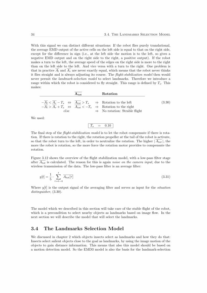
34 3.4. The Landmarks Selection Model
With this signal we can distinct different situations: If the robot flies purely translational,the average EMD output of the active cells on the left side is equal to that on the right side,except for the difference in sign (i.e., at the left side the motion is to the left, so gives anegative EMD output and on the right side to the right, a positive output). If the robotmakes a turn to the left, the average speed of the edges on the right side is more to the rightthan on the left side to the left. And vice versa with a turn to the right. One problem isthat in practice Al and Ar are never exactly equal, which means that the robot never thinksit flies straight and is always adjusting its course. The flight-stabilization model then wouldnever permit the landmark-selection model to select landmarks. Therefore we introduce arange within which the robot is considered to fly straight. This range is defined by Ts. Thismakes:
Atot Rotation
−Al < Ar − Ts ⇔ Atot > Ts ⇒ Rotation to the left−Al > Ar + Ts ⇔ Atot < −Ts ⇒ Rotation to the right
else ⇒ No rotation: Strable flight
(3.30)
We used:
Ts = 0.10
The final step of the flight-stabilization model is to let the robot compensate if there is rota-tion. If there is rotation to the right, the rotation propeller at the tail of the robot is activate,so that the robot turn to the left, in order to neutralize the rotation. The higher |Atot |, themore the robot is rotation, so the more force the rotation motor provides to compensate therotation.
Figure 3.12 shows the overview of the flight stabilization model, with a low-pass filter stageafter Atot is calculated. The reason for this is again noise on the camera input, due to thewireless transmission of the data. The low-pass filter is an average filter:
y[t] =15·
t∑τ=t−4
Atot[τ ] (3.31)
Where y[t] is the output signal of the averaging filter and serves as input for the situationdistinguisher, (3.30).
The model which we described in this section will take care of the stable flight of the robot,which is a precondition to select nearby objects as landmarks based on image flow. In thenext section we will describe the model that will select the landmarks.
3.4 The Landmarks Selection Model
We discussed in chapter 2 which objects insects select as landmarks and how they do that:Insects select salient objects close to the goal as landmarks, by using the image motion of theobjects to gain distance information. This means that also this model should be based ona motion detection model. So the EMD3 model is also the basis for the landmark-selection

Chapter 3. A Visual Landmark-Selection Model for Flying Robots 35
model.
Since the robot is flying straight, there is no image flow in the frontal and dorsal part of thevisual field and the image flow is the most obvious in the lateral part. This means that wecan only gain reliable distance information from image flow in the lateral part of the visualfield. For that reason, we used the EMD3-cells in both lateral parts of the camera image.The areas where the cells are located are between −30o and −150o horizontal angle on theleft side and between 30o and 150o on the right side (0o is the front of the robot). Landmarksare only selected by flying forwards (or possibly backwards) and not by flying up or down.This means that we only use horizontally oriented EMD3-cells. Figure 3.13 shows the layoutof the landmark-selection model.
Spatial−Temporal Low−pass Filter
−150o o−30 30 o 150o
Mark Active Cells
Select Landmarks
Acquire Close Object Blobs
EMD3 EMD3Cells Cells
Figure 3.13: The EMD3-cells are placed in the lateral parts of the visual field, with a horizontalorientation. The outputs of the cells are filtered in both the temporal and the spatial domain. Cellsthat register image motion that is fast enough (i.e., an object that is close enough) are marked asactive cells. These loose active cells form groups. With a clustering algorithm called blob coloring,blobs are acquired. These blobs correspond with objects that are close to the robot. So they areselected as landmarks. With the selection, the size and position of the blobs in the image is saved,together with the average EMD output of the entire blobs which gives distance information about thelandmark. At last, the part of the image in which the blobs is lain is saved as a PPM-image. Thisimage represents the color and shape of the landmark.
The outputs of the EMD-cells are passed through a low-pass filter, which smoothes the sig-nals both in the space and time domain. The reason for this is, as in the flight-stabilizationmodel, sensory noise. Smoothing in only the time domain is not sufficient, because the theedges in the image move. So at one time step an edge is at one EMD-cell and the next timestep at another. This means that there is no distinction between a change in pixel luminancedue to a moving edge and a change due to noise when only filtering in the time domain isused. We want to ’track’ the edge during for a short time. This is the reason that filteringin the space domain is added.
The spatial-temporal filter consists of a 2D averaging filter in the spatial domain and an
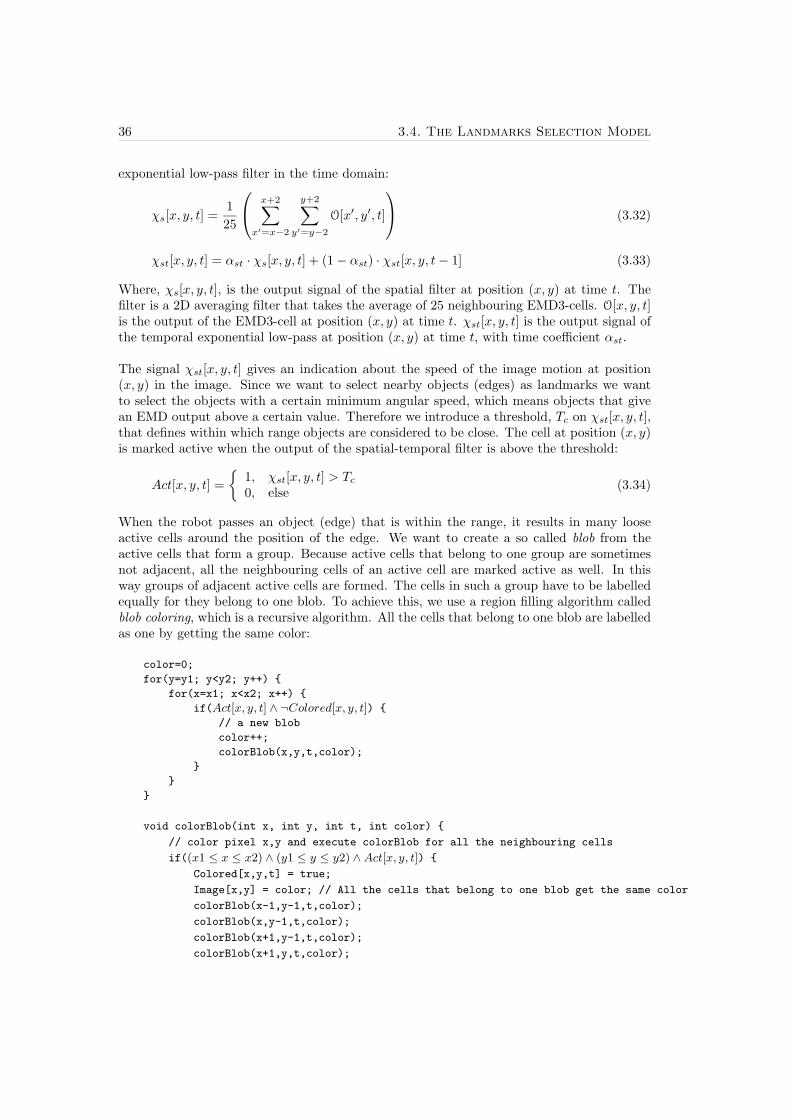
36 3.4. The Landmarks Selection Model
exponential low-pass filter in the time domain:
χs[x, y, t] =125
x+2∑x′=x−2
y+2∑y′=y−2
O[x′, y′, t]
(3.32)
χst[x, y, t] = αst · χs[x, y, t] + (1− αst) · χst[x, y, t− 1] (3.33)
Where, χs[x, y, t], is the output signal of the spatial filter at position (x, y) at time t. Thefilter is a 2D averaging filter that takes the average of 25 neighbouring EMD3-cells. O[x, y, t]is the output of the EMD3-cell at position (x, y) at time t. χst[x, y, t] is the output signal ofthe temporal exponential low-pass at position (x, y) at time t, with time coefficient αst.
The signal χst[x, y, t] gives an indication about the speed of the image motion at position(x, y) in the image. Since we want to select nearby objects (edges) as landmarks we wantto select the objects with a certain minimum angular speed, which means objects that givean EMD output above a certain value. Therefore we introduce a threshold, Tc on χst[x, y, t],that defines within which range objects are considered to be close. The cell at position (x, y)is marked active when the output of the spatial-temporal filter is above the threshold:
Act[x, y, t] ={
1, χst[x, y, t] > Tc0, else (3.34)
When the robot passes an object (edge) that is within the range, it results in many looseactive cells around the position of the edge. We want to create a so called blob from theactive cells that form a group. Because active cells that belong to one group are sometimesnot adjacent, all the neighbouring cells of an active cell are marked active as well. In thisway groups of adjacent active cells are formed. The cells in such a group have to be labelledequally for they belong to one blob. To achieve this, we use a region filling algorithm calledblob coloring, which is a recursive algorithm. All the cells that belong to one blob are labelledas one by getting the same color:
color=0;
for(y=y1; y<y2; y++) {
for(x=x1; x<x2; x++) {
if(Act[x, y, t] ∧ ¬Colored[x, y, t]) {
// a new blob
color++;
colorBlob(x,y,t,color);
}
}
}
void colorBlob(int x, int y, int t, int color) {
// color pixel x,y and execute colorBlob for all the neighbouring cells
if((x1 ≤ x ≤ x2) ∧ (y1 ≤ y ≤ y2) ∧Act[x, y, t]) {
Colored[x,y,t] = true;
Image[x,y] = color; // All the cells that belong to one blob get the same color
colorBlob(x-1,y-1,t,color);
colorBlob(x,y-1,t,color);
colorBlob(x+1,y-1,t,color);
colorBlob(x+1,y,t,color);

Chapter 3. A Visual Landmark-Selection Model for Flying Robots 37
colorBlob(x+1,y+1,t,color);
colorBlob(x,y+1,t,color);
colorBlob(x-1,y+1,t,color);
colorBlob(x-1,y,t,color);
}
}
So a blob is a group of cells that give an EMD output above the threshold and so correspondwith an objects that passes the robot at a short distance. In other words, the blob representsa landmark.
In section 2.2.3 we concluded that bees learn the apparent size of the landmark, the positionof the landmark on the retina, some distance information, the color of the landmark and theshape of the landmark. We want our model to learn the same cues about the landmarks.We learn the size by saving the width and height of the blob. De position on the retina isrepresented by the position of the center of the blob in the camera image. The average EMDoutput of the entire blob gives information about the distance of the landmark. And the colorand shape information is learnt by saving that part of the image which includes the blob.This gives a small image of the landmark in PPM format.
With the saving of this information about the landmark we say that the landmark is selected.The information is required, in order to be able to localize the landmarks during the land-mark navigation (e.g. as described by the snapshot model).
To complete the landmark-selection model, we have to establish the threshold, Tc, whichdetermines the maximum range of ’nearby’ objects. We want to classify objects within arange of 2.00m as being close, these objects have to be selected as landmarks. Objects at adistance ≥ 2.00m should not be selected. Tests with this model implemented on the flyingrobot result in a threshold that satisfy the requirement:
Tc = 0.18
The objects that are selected as landmark should have a salient property, otherwise its notpossible to find the landmark back. This model will take care of this, since it is inherent tothe EMD model: The motion of objects that are not salient (enough), have unclear edgesand will not be detected by the EMD3-cells, because of the threshold on the high-pass filter(3.10). Therefor these objects will not be selected as landmarks.
3.5 Conclusion
In this chapter we described a model of the learning phase of landmark navigation. In thisphase, the landmarks in the unknown environment are learnt, so that the robot is able toreturn to that location. We proposed a model to select objects close to the robot as land-marks. To be able to create this model we had to make a model that stabilizes the course ofthe robot. A nice aspect about these models is that they both rely on the same underlyingmotion detection model, the EMD3 model. In the flight-stabilization model the EMD3-cellsin the frontal and dorsal part of the visual field are used whereas the landmark-selectionmodel uses the cells in the lateral parts. The beauty of the underlying EMD3 model is that

38 3.5. Conclusion
it can also be used to avoid objects, to regulate the speed and altitude of the robot, to pro-vide a safe landing and for odometry (see section 2.1.3). Implementations of some of thesepossibilities have been done by [Mura and Franceschini, 1994] (speed and altitude) [Netterand Franceschini, 1999] (altitude) [Srinivasan, Zhang, and Chahl, 2001] (save landing) and[Iida and Lambrinos, 2000; Franceschini, Pichon, and Blanes, 1991](odometry).
So, the underlying EMD model can be reused for different purposes. Being able to reusea basic circuit is very important for flying agents, since there are normally very strict con-straints on the amount of payload the agent can carry. Moreover, reusing the same circuitis an advantage from a computational point of view, since one underlying model is moreefficient and requires less computational power. The same principle of reusing basic circuitfor different purposes is also found in nature. Lehrer [1998] shows that honeybees use imageflow information in different eye regions for different purposes.
In the next chapter we will describe some experiments to test the models and we will showthe results of these experiments, with which we can discuss the practicability of the models.

Chapter 4
Experiments
In this chapter we will explain the experiments with the models described in the previouschapter, implemented on the flying robot, Melissa. We will show the experimental setupand the results of the experiments with both the flight-stabilization model and the landmark-selection model.
4.1 The Flight-Stabilization Experiment
The flight-stabilization model as described in section 3.3 is implemented on the flying robot.The experiment in this section is performed, to test whether the model was capable in lettingthe robot fly a straight course, in such a way that the landmark-selection model can selectlandmarks based on image flow.
z xy10 m
0.9 m
Figure 4.1: An overview of the experimental setup of the flight-stabilization experiment. The robotflies approximately 10 meters. During that flight the position is observed by two cameras, looking inthe direction of the flight. By performing stereo vision, the position of the robot in the 3D space isobtained. This shows the degree of stabilization of the robot’s course.
4.1.1 The Experimental Setup
Figure 4.1 shows the setup of the flight-stabilization experiment. The robot is expected to flyapproximately 10 meter in a straight line. The flight of the robot is recorded by two cameras,
39

40 4.1. The Flight-Stabilization Experiment
both looking in the direction of the flight. By means of this stereo vision, the trajectory ofthe robot in the 3D space can be observed. We obtain the 3D-coordinates as follows:
Stereo Vision to Obtain the Robot’s Position
From the two camera images, we want to derive the position of the robot in the 3D space.We will explain the geometry behind this localization task.
x1
x + y12 2
x + y + z12 2 2
y + z2 2
α 1β
1
β2
α 2
x cam2
1cam1
(x,y,z)
x−axis
z−axis
y−axis
Figure 4.2: The geometry of the camera setup. α1 and β1 are defined by respectively the horizontaland vertical position of the robot in the first camera image and α2 and β2 by the position in thesecond camera image. With these four parameters, the position of the robot, (x, y, z), in the 3Dspace is derived.
The distance between cam1 en cam2 is 0.9 m. Therefore as we look at Figure 4.2 we see:
x1 + x2 = 0.9 (4.1)
Further more:
tanα1 =x1√y2 + z2
(4.2)
tanα2 =x2√y2 + z2
(4.3)
sinα1 =x1√
x21 + y2 + z2
and sinα2 =x2√
x22 + y2 + z2
(4.4)
sin β1 =z√
x21 + y2 + z2
and sin β2 =z√
x22 + y2 + z2
(4.5)

Chapter 4. Experiments 41
cos β1 =
√x2
1 + y2√x2
1 + y2 + z2and cos β2 =
√x2
2 + y2√x2
2 + y2 + z2(4.6)
Combining (4.2) and (4.3) we get:
x1
tan α1=
x2
tan α2(4.7)
Combining this with (4.1):
x1
tan α1=
0.9− x1
tan α2
x1 · tan α2 = 0.9 · tan α1 − x1 · tan α1
x1(tanα1 + tanα2) = 0.9 · tanα1
x1 =0.9 · tanα1
tanα1 + tanα2(4.8)
Similar to this we can deduce:
x2 =0.9 · tanα2
tanα1 + tanα2(4.9)
This gives us the x-coordinate:
x = x1 − 0.45 and x = 0.45− x2 (4.10)
If we put together (4.4) and (4.5), we get the z-coordinate:
x1
sinα1=
z
sinβ1and
x2
sinα2=
z
sinβ2
z = x1 ·sinβ1
sinα1and z = x2 ·
sinβ2
sinα2(4.11)
And finally the y-coordinate by (4.4) and (4.6):√x2
1 + y2
cosβ1=
x1
sinα1and
√x2
2 + y2
cosβ2=
x2
sinα2√x2
1 + y2 =x1 · cosβ1
sinα1and
√x2
2 + y2 =x2 · cosβ2
sinα2
y =
√(x1 · cosβ1
sinα1
)2
− x21 and y =
√(x2 · cosβ2
sinα2
)2
− x22 (4.12)
The parameters in these equations, α1, β1, α2 and β2, are defined by the horizontal andvertical position of the robot in both camera images.
The cameras have a resolution of 640 × 480. Both cameras have the same horizontal andvertical maximum angle of view. The horizontal angle of view is between −θ1 and θ1 and inthe vertical direction between θ2 and −θ2. The total angle of view is equally divided amongall the pixels, so each pixel covers an angle of 2θ1/640 in the horizontal direction and 2θ2/480vertically.

42 4.1. The Flight-Stabilization Experiment
pixel coordinates
pixelcoord.
θ
θ
1
2
00
480
640
−θ−θ 2
1
0
0
view angle
viewangle
x c
cy
Figure 4.3: The camera image of the two cameras that are used for stereo vision has a resolution of640 × 480 pixels. The figure show the pixel coordinates on the top and left axes and the associatedangles on the bottom and right axes.
If the position of the robot in the image of camera i measured in pixels is (xci, yci), we canderive:
αi = (xci − 320) · θ1
320(4.13)
βi = (yci − 240) · − θ2
240(4.14)
Every 0.5 s the position of the robot is obtained by equations (4.10), (4.11) and (4.12). Thisresults in a series of (x, y, z) coordinates, which represents the flight trajectory of the robot.
The task for the robot in this experiment is to fly a straight course over a distance of 10meters, using the model described in section 3.3. With this stereo vision setup, the trajectoryof the robot during the flights is obtained. In the next section we will show the results ofeight trials.
4.1.2 The Results
Figure 4.4 and Figure 4.5 show the result of eight flight-stabilization trials. Figure 4.4 showsthe trajectories of the robot in the xy-plane, where the y-axis is in the direction of the flightand on the x-axis are the deviations of the robot to the left and right. So this can been seenas viewed from above. Figure 4.5 gives the view from the side. Here are the deviations ofthe robot upwards and downwards shown on the z-axis.If we look at Figure 4.4 and Figure 4.5, we see that, although the robot is flying quite straightduring the trials, the robot sometimes slightly deviates from the straight course. This meansthat the robot is sometimes making a slow turn to the left or to the right or is slowly goingup or down. We have to analyse the data to answer the next questions: What is the meanrotational velocity of the robot during these trials? And: Can we consider this as a stableflight, or does the rotation strongly influences the landmark selection task?

Chapter 4. Experiments 43
-4
-2
0
2
4
1 2 3 4 5 6 7 8 9 10
x�
y
Stabilize flight
trial 1trial 2trial 3trial 4trial 5trial 6trial 7trial 8
Figure 4.4: This graph shows the trajectory of the robot during the eight trials in the yx-plane. They-axis is the direction in which the robot flies. y is the distance in meters. On the x-axis are thedeviation to the left and right given, also measured in meters. x > 0 means a deviation to the leftand x < 0 to the right. So we can see this graph as viewed from above.
-4
-2
0
2
4
1 2 3 4 5 6 7 8 9 10
z (m
)
y (m)
Stabilize flight
trial 1trial 2trial 3trial 4trial 5trial 6trial 7trial 8
Figure 4.5: The trajectory of the robot during the same eight trials as viewed from the side. They-axis is again the direction in which the robot flies and the z-axis gives the deviation of the robotupwards and downwards. z > 0 is up and z < 0 is down. Both variables are measured in meters.
Performance analysis
To answer the question what the mean rotational velocity of the robot is during 22 seconds offlight, we have to determine the mean rotation of the robot during the flight. In other words,the difference in orientation at the beginning and at the end of the flight. To calculate this,we use the assumption that the robot rotates with a fixed rotational velocity, which meansthat the trajectory of the robot describes a part of a circle. The radius of that circle dependson the distance of the flight and the deviation of the robot from the straight course. From

44 4.1. The Flight-Stabilization Experiment
r
r
d
αβ
T
x
Figure 4.6: What is the rotation of the robot during the flight? The flight of the robot is approximatedby assuming that it rotates with a fixed rotational speed, so the trajectory describes a part of a circle,shown by T . d is the displacement in meters of the robot at the end of the flight and r is the radiusof the circle. α is the difference in orientation of the robot between the beginning and the end of theflight.
Figure 4.6 we see:
(r − d)2 + x2 = r2 ⇔ r =d2 + x2
2d(4.15)
where r is the radius of the circle, x is the distance of the flight and d is the deviation at theend of the flight that the robot made. Next, the angle β can be calculated:
β = arccos(x
r) (4.16)
Finally the the difference in orientation, α, can be calculated:
α =12π − β ⇔ α =
12π − arccos(
xd2+x2
2d
) (4.17)
With this formula and the results of the experiments we can calculate the yaw rotation (e.i.,the rotation to the left and right). The distance of the flight is x = 9.0 m. The meandeviation at the end of the flight is the average over all trials, i, of the absolute deviations,di: dy = 1
8
∑8i=1 |di| = 0.71 (σ2 = 0.24). We can now calculate the difference in orientation
during the whole flight, αy = 0.157 rad. Since the duration of the flight was 22 s, the meanrotational velocity is:
ωy = 0.157/22 = 7.14 · 10−3 rad/s (4.18)
where ωy is the rotational velocity of the yaw. This corresponds to 7.14 ·10−4rad/frame witha frame rate of 10 Hz. And the horizontal displacement of the environment in the cameraimage due to the rotation, measured in pixels is 240
2π · 7.14 · 10−4 = 0.027 pixels/frame.
On a similar way the rotational velocity of the pitch (e.i., rotational velocity up and down)can be calculated. The mean deviation in the yz-plane is dp = 0.32 (σ2 = 0.053). This gives:αp = 0.071 rad and a mean rotational velocity of the pitch:
ωp = 3.23 · 10−3 rad/s (4.19)
Chapter 4. Experiments 45
The height of the camera image is 90 pixels, which covers 100o or 0.56π rad of the visual field.So ωp corresponds with a vertical displacement in the camera image of 90
0.56π · 3.23 · 10−4 =0.017 pixels/frame.
Is the observed flight a stable flight? This depends under which assumptions the fight isconsidered stable, which depends on the purpose of the flight. For instance, the assumptionunder which the flight of a homing missile is considered stable is when the missile absolutelydoes not deviate from the straight course. The purpose of the stable flight of our robot is toselect relevant landmarks based on image flow. For this purpose, we assume that the flight isstable when the deviation of the robot from the straight course does not strongly influencesthe functionality of the landmark-selection model.
We pointed out that the robot slightly rotates during the flight. What is the influence of thisrotation? When the robot passes an object at 2.00 m, this object has a horizontal angularvelocity of 0.20 rad/s. Because of the yaw rotation of the robot this is observed by the cam-era as an angular velocity between 0.1929 rad/s and 0.2071 rad/s, which corresponds to anobject at a distance between 2.07 m and 1.93 m. This is an error range of 3.5%. (The errorof objects farther from the robot is slightly more and the error of closer object is less). Sincewe want to make a separation between nearby and distant objects, and we do not want toknow the exact distance, an error of 3.5% is good enough and absolutely does not influencethe functionality of the landmark-selection model.
The pitch rotation is even less than the yaw rotation. Moreover the pitch rotation of therobot works on the vertical axis of the camera image and does not change the horizontalangular velocity of objects, which we use in the landmark-selection model.
In the light of the experiment discussed in this section, we can conclude that the flight-stabilization model successfully stabilizes the flight of the robot for the purpose of landmarkselection based on image flow. With the stable flight of the robot that this model provides,the landmark-selection model can select landmarks based on image flow.
4.2 The Landmark-Selection Experiment
In this model we discus the experiments with the model for the selection of landmarks,described in section 3.4, that we implemented on the flying robot.
4.2.1 The Experimental Setup
To obtain statistical evidence, an experiment has to be performed a few times under the sameconditions. The problem with a freely flying robot is that there are always some differencesin the flights of the robot and so the experiments are taken under dissimilar conditions. Forthat reason we created a rails on which the robot can move (see Figure 4.7), every timeexactly the same trajectory, with the same speed and starting at the same moment.
The gondola of the robot moves over the rails with the same speed as the freely flying robotflew during the flight-stabilization experiment. During a ’flight’, the gondola passes land-marks, placed at one side of the rail at different distances from the robot. We used onlyone lateral side out of practical reasons. The other lateral part would give exactly the same

46 4.2. The Landmark-Selection Experiment
Figure 4.7: The setup of the landmark-selection experiments. The gondola of the robot moves overa rails, pulled by a motor. The speed of the robot is equal to the speed of the freely flying robot at theflight-stabilization experiment. Landmarks were placed at the side of the rail.
results, except that the direction of the image flow would be reversed.
In the first experiment a black cylindrical landmark is placed with length 1.00 m and Ø =0.25 m at different distances from the robot (0.50, 1.00, 1.50, 2.00, 2.50 and 3.00 m). The hy-pothesis is that the model implemented on the robot selects the landmarks within the rangeof 2.00 m (e.i., at 0.50, 1.00 and 1.50m) and does not select the landmarks outside that range(e.i., at 2.00, 2.50 and 3.00m). This hypothesis is discussed in section 3.4.
Experiment I Experiment II Experiment III
Figure 4.8: In the first experiment a black landmark of length 1.00 m and Ø = 0.25 m is placed at0.50, 1.00, 1.50, 2.00, 2.50 and 3.00 m from the robot. Smaller (Ø = 0.15 m) and bigger (Ø = 0.50 m)black landmarks are used in the second experiment. Again the landmarks are placed on differentdistances from the robot. In the last experiment a black and a red landmark with Ø = 0.25 m areused, also placed on different distances. In all these experiments one landmark per trial is used.
The distance of the landmark can be obtained in two ways. Based on the apparent speed
Chapter 4. Experiments 47
of the landmark and based on the size. Because in this model the distance has to be ob-tained by the apparent speed of the object, a second experiment is set up, to see if the sizeof the landmark influences the selection. The experiment is equal to the previous, exceptthat we performed it with a smaller landmark with Ø = 0.15 m and a bigger landmark withØ = 0.50 m. The hypothesis is that the model is invariant to the size of the landmarks andwill select those landmarks that are within the range of 2.00 m.
Does the color of the landmarks matter? In section 3.2.2 we changed the EMD model sothat it should be invariant to the color of object. In this third experiment we test if the colorof the landmark really does not influences the landmark selection model. Again the experi-ment is identical to the previous, but now we compared a black landmark with Ø = 0.25 mwith a red landmark of the same size. Here the hypothesis is that the model is invariant tothe color of the landmarks and will select those landmarks that are within the range of 2.00 m.
In all the experiments four trials are taken under the same conditions. See Figure 4.8 for anoverview of the three experiments.

48 4.2. The Landmark-Selection ExperimentT
ime
d2.
2s
2.6
s3.
0s
3.4
s3.
8s
0.50
m
1.00
m
1.50
m
2.00
m
2.50
m
3.00
m
Fig
ure
4.9:
Th
eca
mer
aim
age
sw
hen
the
robo
tpa
sses
the
lan
dm
ark
s.T
he
ima
ges
at
diff
eren
tpo
ints
inti
me
are
pla
ced
ho
rizo
nta
l.O
nth
eve
rtic
al
axi
sis
the
vari
ati
on
ind
ista
nce
fro
mth
eL
Mto
the
robo
t,d
.T
he
colo
red
blo
bsd
epic
tth
ese
lect
edla
nd
ma
rks.
Th
em
odel
lea
rns
the
lan
dm
ark
sby
savi
ng
tho
sepa
rts
of
the
cam
era
ima
gew
her
eth
ebl
ob
islo
cate
d.
De
arr
ow
sa
bove
the
ima
gein
dic
ate
the
posi
tio
no
fth
ela
nd
ma
rkin
the
ima
ge.

Chapter 4. Experiments 49
4.2.2 Experiment I
The result of the first experiment is shown in Figure 4.9. The figure shows the camera imageswhen the robot passes the landmark, at 2.2, 2.6, 3.0, 3.4 and 3.8 seconds from the beginningof the flight, for all distances. The brightly colored areas in the images are the blobs thatare obtained with the method described in section 3.4. When a blob is shown, it means thatthere is a landmark-selected. The part of the camera image where that blob is located issaved as an image in PPM format.
Figure 4.9 clearly show that the object is selected as landmark when it is within the rangeof 2.00 m and that it is not selected as a landmark when the object is placed at 2.00 m orfurther. Only In the image with the landmark at distance 2.00 m at 2.6 s, the object isselected as landmark. But since this is a single failure, not a regularity and the object is notselected in succession, it is not considered a landmark.
Figure 4.10 shows the same results, but in a different representation. The time is placed onthe horizontal axis. Time is measured here in camera frames, every frame is 0.1 s. On thevertical axis are the smoothed values of the average EMD outputs of all the EMD3-cells inthe blobs shown. These values are also the average over four trials. The different lines indi-cate the different distances of the object from the robot. The graphs of the objects withinthe range of 2.00 m show high values, which suggests again that the object is selected aslandmark. The graph is positioned higher when the object is closer to the robot, which iscorrect, since the vertical axis gives an approximation of the angular speed of the object.
0
0.05
0.1
0.15
0.2
0.25
0.3
0 10 20 30 40 50 60 70
Ave
rage
EM
Dou
tput
�
Time in frames (1 frame = 0.1 sec)
Average EMDoutput from cells in the active blobs. Diameter object 25cm, color black
LM at 50cmLM at 100cmLM at 150cmLM at 200cmLM at 250cmLM at 300cm
Figure 4.10: The horizontal axis gives the time measured in camera frames. 1 frame = 0.1 s.On the vertical axis is the average EMD output of all the EMD3-cells in the blobs given. Thisis also the average over four trials. The figure shows six graphs with the object positioned at0.50, 1.00, 1.50, 2.00, 2.50 and 3.00 m from the robot. The object is black with length 1.00 m andØ = 0.25 m. The graphs are smoothed with a moving average filter.
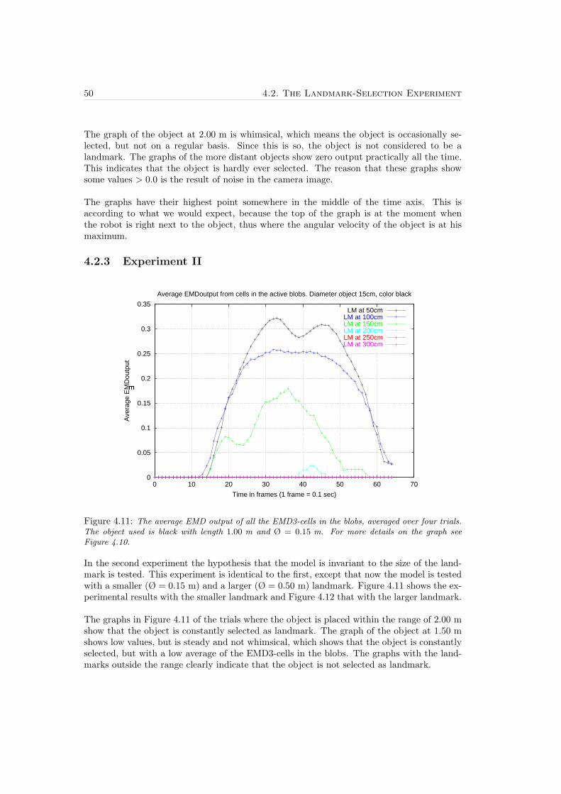
50 4.2. The Landmark-Selection Experiment
The graph of the object at 2.00 m is whimsical, which means the object is occasionally se-lected, but not on a regular basis. Since this is so, the object is not considered to be alandmark. The graphs of the more distant objects show zero output practically all the time.This indicates that the object is hardly ever selected. The reason that these graphs showsome values > 0.0 is the result of noise in the camera image.
The graphs have their highest point somewhere in the middle of the time axis. This isaccording to what we would expect, because the top of the graph is at the moment whenthe robot is right next to the object, thus where the angular velocity of the object is at hismaximum.
4.2.3 Experiment II
0
0.05
0.1
0.15
0.2
0.25
0.3
0.35
0 10 20 30 40 50 60 70
Ave
rage
EM
Dou
tput
�
Time in frames (1 frame = 0.1 sec)
Average EMDoutput from cells in the active blobs. Diameter object 15cm, color black
LM at 50cmLM at 100cmLM at 150cmLM at 200cmLM at 250cmLM at 300cm
Figure 4.11: The average EMD output of all the EMD3-cells in the blobs, averaged over four trials.The object used is black with length 1.00 m and Ø = 0.15 m. For more details on the graph seeFigure 4.10.
In the second experiment the hypothesis that the model is invariant to the size of the land-mark is tested. This experiment is identical to the first, except that now the model is testedwith a smaller (Ø = 0.15 m) and a larger (Ø = 0.50 m) landmark. Figure 4.11 shows the ex-perimental results with the smaller landmark and Figure 4.12 that with the larger landmark.
The graphs in Figure 4.11 of the trials where the object is placed within the range of 2.00 mshow that the object is constantly selected as landmark. The graph of the object at 1.50 mshows low values, but is steady and not whimsical, which shows that the object is constantlyselected, but with a low average of the EMD3-cells in the blobs. The graphs with the land-marks outside the range clearly indicate that the object is not selected as landmark.

Chapter 4. Experiments 51
0
0.05
0.1
0.15
0.2
0.25
0 10 20 30 40 50 60 70
Ave
rage
EM
Dou
tput
�
Time in frames (1 frame = 0.1 sec)
Average EMDoutput from cells in the active blobs. Diameter object 50cm, color black
LM at 50cmLM at 100cmLM at 150cmLM at 200cmLM at 250cmLM at 300cm
Figure 4.12: The average EMD output of all the EMD3-cells in the blobs, averaged over four trials.The object used is black with length 1.00 m and Ø = 0.50 m. For more details on the graph seeFigure 4.10.
Figure 4.13: A black object withØ = 0.50 m at 0.50 m distance isselected as two landmarks.
The graphs in Figure 4.12 show the same results asthe graphs in the previous figure. The object is se-lected within the range of 2.00 m and not outside thatrange. Only the graph with the object at 3.00 m showsan unexpected result. The object is a few times se-lected, but again not regular enough to label it a land-mark.
Figure 4.13 shows how the bigger landmarks are selectedwhen they are close to the robot. Unlike in the case of
the smaller landmarks in the previous experiments, the object is now select as two distinctlandmark. One at the left edge and one at the right. This is a logical result from the factthat the underlying EMD model basically is a moving edge detector.
From these results we can conclude that the model for landmark selection is not influencedby the size of the object. In both the case of a smaller and a larger object, the model onlyselects the objects with in the 2.00 m range as landmarks.
Figure 4.14 puts together the graphs of the black object with Ø = 0.15 m, Ø = 0.25 m andØ = 0.50 m at 0.50 m from the robot. What is notable is that the average EMD outputis higher when the size of the object is smaller. We can explain this from the remark insection 3.2.2, that the EMD model is sensitive to the spatial frequency of objects. Thesmaller an object, the closer its two edges are to each other, the higher the output of theEMD cell when the second edge passes.

52 4.2. The Landmark-Selection Experiment
0
0.05
0.1
0.15
0.2
0.25
0.3
0.35
0 10 20 30 40 50 60 70
Ave
rage
EM
Dou
tput
�
Time in frames (1 frame = 0.1 sec)
Average EMDoutput from cells in the active blobs. The object at 50 cm, color black.
Diameter 15cmDiameter 25cmDiameter 50cm
Figure 4.14: The average EMD output of all the EMD3-cells in the blobs, averaged over fourtrials. The graphs show the results when using objects of different sizes, with length 1.00 m andØ = 0.15, 0.25 and 0.50 m, at 0.50 m from the robot.
4.2.4 Experiment III
In the last experiment, the hypothesis that the landmark-selection model is invariant to thecolor of the object is tested. A red object of the same size as the black object in experimentI is used. Figure 4.15 shows the results of this experiment. Again we see the same results asin the previous experiments. The nearby objects are selected continuously and the fartherobjects are not significantly selected as landmarks.
In Figure 4.16, we compare the results of the experiment with the black and red landmark,both of the same size and both at a distance of 0.50 m. What we see is that the top of bothgraphs is approximately equally high, but that the graph of the red object starts to go uplater in time and starts to go down earlier in time. In other words the angle at which thered object is recognizable by the model is smaller than that of the black object. The reasonfor this is that at a greater angle, the luminance of the red object does not differ enoughfrom the luminance of the background in order for the EMD model to detect the motion.The difference between the two luminances is then below the threshold, Tλ, of equation (3.10).
However, except from the fact that the red object is selected a little later, we can concludethat the landmark-selection model perfectly selects objects of different colors when they arewithin the range of 2.00 m. The results show that the model is invariant to the color ofobjects.

Chapter 4. Experiments 53
0
0.05
0.1
0.15
0.2
0.25
0 10 20 30 40 50 60 70
Ave
rage
EM
Dou
tput
�
Time in frames (1 frame = 0.1 sec)
Average EMDoutput from cells in the active blobs. Diameter object 25cm, color red
LM at 50cmLM at 100cmLM at 150cmLM at 200cmLM at 250cmLM at 300cm
Figure 4.15: The average EMD output of all the EMD3-cells in the blobs, averaged over four trials.The object used is red with length 1.00 m and Ø = 0.50 m. For more details on the graph seeFigure 4.10.
0
0.05
0.1
0.15
0.2
0.25
0.3
0 10 20 30 40 50 60 70
Ave
rage
EM
Dou
tput
�
Time in frames (1 frame = 0.1 sec)
Average EMDoutput from cells in the active blobs. Diameter object 25 cm, distance 50cm
BlackRed
Figure 4.16: The average EMD output of all the EMD3-cells in the blobs, averaged over four trials.The graph shows the results when using a black and a red object with length 1.00 m and Ø = 0.50 m,at 0.50 m from the robot.

54 4.3. Conclusions
4.3 Conclusions
In this chapter we performed some experiments with the model of the learning phase oflandmark navigation, which consists of the two models created in chapter 3. In the first ex-periment we tested the course stabilization model that is based on stabilization mechanismsfound in insects. From the results we see that the model is able to stabilize the course of therobot more than sufficient for the landmark-selection model to select landmarks based on theimage motion of objects. So we can conclude that we created a good working stabilizationmodel, that is based on the same underlying principles as insects use for the stabilization oftheir course, which we discussed in chapter 2.
The second set of experiments was to test the landmark-selection model. As the flight-stabilization model, this model is also based on methods adapted from biological studies.The results from these experiments show that the model is able to select nearby objects aslandmarks, based on the image flow of the objects, which is produced by the ego-motion ofthe robot. The underlying EMD model makes a good estimation of the distance towards theobjects, and the landmark selection model selects those objects that are within the range of2.00 m from the robot. The results of the experiments also show that the model is invariantto the size and color of the objects. So we can conclude that we created a working landmarkselection model that is biologically plausible.

Chapter 5
Discussion
In this thesis we have attempted to model the learning phase of landmark navigation. Themodel consists of two models; the flight-stabilization model and the landmark-selectionmodel. Both models are the result of biorobotic research. Findings from biological stud-ies on flying insects are used to build these models for the control of the freely flying robot.
The experiments performed with the flight-stabilization model show that we successfullycreated a biologically plausible model for the stabilization of the course of the robot. Theresults of the landmark selection experiments show that we also succeeded in building a modelthat selects landmarks for the use of landmark navigation, in the same manner as honeybeeswhen they learn about a location that they wish to revisit.
A Single Theoretical and Technical Foundation
A nice property of both the flight-stabilization model and the landmark-selection model forrobots is that they are both based on the same underlying motion detection model; the EMDmodel. EMD3-cells in the frontal and dorsal part of the visual field are used for the stabi-lization of the flight and cells in the lateral parts are used for the selection of nearby objectsas landmarks. Moreover, the EMD model can also serve as the basic circuit for other formsof movement control, such as controlling the altitude of the robot, by using the caudal part ofthe visual field [Netter and Franceschini, 1999; Mura and Franceschini, 1994], controlling thespeed of the robot by using the caudal, cranial and/or lateral parts [Mura and Franceschini,1994], avoiding obstacles by using frontal part, obtaining a save landing by using the caudalpart [Srinivasan, Zhang, and Chahl, 2001] and flying through the middle of a gap (lateral).Besides that, the EMD model can also be used for odometry, by using the caudal, cranialand/or lateral part of the visual field [Iida and Lambrinos, 2000; Franceschini, Pichon, andBlanes, 1991]. See section 2.1.3 for the biological backgrounds.
Being able to use the same basic circuit is an advantage for the computational power thatis required to control the robot. There is also an advantage when the control of the robotis modeled in analog hardware, like in [Moller, 1999] and [Franceschini, Pichon, and Blanes,1992]. A shared basic EMD circuit then saves weight in the amount of payload, which is abenefit to flying robots.
The EMD itself is a computationally cheap motion detector. In both models we used manyEMDs, serially implemented, which obviously slows down the process. However, a nice
55
56
property of the EMD model is that it is an independent local motion detector, which givesthe possibility of parallel processing. If the array of EMDs, used in both models, wereimplemented as a parallel sensing device, the speed of processing of both models wouldincrease greatly.
Distance Estimator
An important part of the landmark-selection model is that distances towards objects canbe estimated, based on the image flow of the objects. This strategy is also found in thelocust [Sobel, 1990]. When the locust wants jump on an object, it looks at the object andstarts peering, e.g., it moves its head from left to right, while fixating the orientation of thehead [Collett, 1978]. By doing this, the locust obtains the motion of the object, which givesinformation about the distance. This information is used in order to jump on the object.But when the object is moved during the peering, the locust can be fooled. When the ob-ject is moved opposite to the movement of the locust’s head, the motion of the object ishigher and the locust thinks that the object is closer. Therefore the locust jumps in front ofthe object, instead of on the object. When the object is moved with the movement of thehead, but slower, the locust jumps too far. This experiment shows that the locust estimatesthe distance towards the object, based on the speed of image flow of the object when peering.
This example of distance perception in the locust again shows that the model is biologicallyplausible, but what is the advantage for roboticists? Why should they use this strategy toobtain the distance towards object, instead of using other techniques like, laser range finding,sonar or stereo-vision? The big advantage of our method is that we use only one single sen-sor, with which we can attain movement control of the robot, selection of the landmarks andnavigation on these landmarks, namely the omni-directional camera. Using only one sensoris again a profit for the robot’s amount of payload.
An advantage of the other methods to gain distance information - like laser, sonar and stereo-vision - is that they are more precise in estimating the distance than our model. But sincewe only want a rough estimation to know if an object is close or far, our model is accurateenough for the task.
Landmark Selection and the Snapshot Model
We already mentioned that the models proposed in this thesis provide the learning phaseof the landmark navigation. The models enable the robot to learn an unknown location, sothat the robot is able to return to that location.
The ability to return the learnt goal location (i.e., landmark navigation) is modeled in thesnapshot model, which we discussed in section 2.1.2. In [Moller, 2000] a more economi-cal model, based on the snapshot model is proposed, the Average Landmark Vector (ALV)model. Both the snapshot model and the ALV model do not provide the learning phase. Ifwe combine our model with one of these models, we have a complete model that providesthe robot with the ability to learn an unknown site and to return to this site by navigatingon the learnt landmarks.
Using the Global Positioning System (GPS), would be another option to navigate the robot toa given location. However relying on an external system makes the system not autonomous
Chapter 5. Discussion 57
and it does not conform to the philosophy of biorobotics, since GPS is not biologicallyplausible. Moreover, such an external system is not everywhere available. Robots on Mars,for instance, can not rely on the GPS system, as yet.
Shortcomings
The model that we proposed has a few shortcomings, which we would like to discuss here.
In the first place is our model not able to select landmarks in the entire surroundings of thegoal location. The robot only flies forward and selects the landmarks in the lateral parts ofthe visual field. To learn the entire environment, the objects in the frontal and dorsal part ofthe should also be evaluated. During the TBL phase that honeybees perform, the bee solvesthis problem by hovering from left to right as well as moving backwards. Our robot is notable to hover from left to right because of physical limitations. A different strategy shouldbe used to select landmarks in the frontal and dorsal parts of the visual field.
The second shortcoming is what we discussed before: Our model only provides the learningphase of landmark navigation. It is not able to navigate on the selected landmarks. To realizethis, we should couple our model to the snapshot model or the ALV model.
A Related Study
In [Bianco, 1998] and [Lehrer and Bianco, 2000] another model is proposed for automaticlandmark selection and navigation for mobile robots, using a TBL-phase: Landmarks areselected by first testing the static and then the dynamic reliability. A landmark is a squareof 80 × 80 pixels in a 640 × 480 image. Static reliable landmarks are squares that have ahigh local uniqueness. An equal number of landmarks is chosen from each sector of the visualfield. Thereupon the robot performs a TBL phase. It drives from the goal location and movesfrom left to right, constantly pointing the camera at the goal location. Along the way, thepotential landmarks are tracked and their uniqueness is tested. Potential landmarks with anevaluation above a threshold at the end of the TBL are chosen as landmarks. In this way, themodel selects objects in the environment that are noticeable, in other words salient objects,as landmarks.
During the landmark navigation task, the landmarks are localized in the current view byusing a brute force search. The stored images of the landmarks are cross-correlated with allpossible parts in the current view, whereby the size of the stored image of the landmark is alsoenlarged and reduced. The position and the size of the landmark that give the best match isthan taken. By comparing this with the size and position of the landmark in the snapshot, atangential and a radial vector is calculated. Adding these vectors of all the landmarks givesa homing vector.
This model resembles the model that we proposed in this thesis. Both models are inspiredby the TBL phase that bees perform to learn an unknown site. But they differ greatly inwhich landmarks are selected and how these landmarks are selected. Bianco’s model chooseslandmarks that are reliable in the sense that they are salient, but the model does not take thedistance of the landmarks into account. Landmarks that are salient, but are positioned farfrom the goal, have a great change to be selected. However, these landmarks are not reliable,since the robot can not use distant landmarks for detailed navigation to the goal location.
58
Our model does take the distance of landmarks into account. The model proposed in thisthesis selects landmarks that are reliable in the sense that they are salient as well as close tothe goal. Furthermore our model and the model of Bianco [1998] differ in the strategy howthe landmarks are selected. Where we choose a biologically inspired method by using thebiologically plausible EMD model to select landmarks based on their image flow, Bianco’smodel uses classical computer vision methods, which are more computational demanding andfar less biologically plausible.

Chapter 6
Conclusion
In chapter 2 we answered the question how insect learn an unknown location in an unknownenvironment. We have described how bees solve this problem by learning the landmarks inthe surroundings. Bees only learn those objects that are salient and near the goal location.They select those objects as landmarks by using the image flow of the objects, inducedby egomotion. To gain reliable distance information from the image flow, the flight of thebee during the selection phase need to be stable. In chapter 3 we proposed a model toimplement this strategy found in bees on an autonomous flying robot. The model consistsof two submodel; a flight-stabilization model and a landmark-selection model. According tothe results of the experiments performed in chapter 4, both models that we presented canbe called successful. The course stabilization model is able to stabilize the flight of the robotin such a way that the distance information gained from the speed of image flow is reliable.The model for landmark selection successfully selects salient objects that are near the goallocation as landmarks, invariant to the size and color of the object.
Future Work
We already pointed out that there are some shortcomings of the model, which are points forfuture work:
The first point is the fact that the model does not enable the robot to select landmarks inthe entire surroundings of the goal. Because of physical limitations, the robot is not able tohover from left to right, and the robot is therefore not able to select landmarks based on theimage flow in the frontal and dorsal part of the visual field. Instead of hovering from left toright, the robot could make a 90o turn and fly straight again. In this way the robot is ableto select the landmarks complete surroundings. However, to make exactly a 90o turn is avery complicated thing to do when the only sensory input is vision provided by the omni-directional camera. To solve this problem, we should think about using compass information,something that bees also use for their navigation (see [Gould, 1980]).
The second subject for future work is coupling either the snapshot model or the ALV modelto our model. The first task to solve is to locate the learnt landmarks in the current viewwhen the robot is displaced from the goal location. The second task to solve is to obtaina displacement vector (or homing vector) from the differences in position and size of thelandmarks in the current view and the landmarks as they are saved at the goal location.Finally the robot should be moved according to the displacement vector.
59
60
When these two point of future work will be realized, a model is completed that learns alocation in an unknown environment and has the ability to return to this location.
Benefits to Biology and Robotics
The presented models are a result of biorobotics research. What is the benefit of this studyto both biology and robotics? For biologists, the successful implementation of the modelson an autonomous flying robot verifies that the biological theories underlying these modelsare plausible. Our study may also give biologists more insight in the landmark navigationtask of insects. The contribution of this study to robotics is that we presented a model thatgives a robot the ability to learn a location in an unknown environment, in order to be ableto return to that location. Moreover, the model has the property that it is computationallycheap and that it requires little carrying capacity, for which reason it is possible to implementon a freely flying robot.

References
Barron, J.L., D.J. Fleet, and S.S. Beauchemin. (1994). Performance of optical flow tech-niques.
Bianco, G. (1998). Biologically inspired visual landmark learning and navigation for mobilerobots. Ph.D. thesis, University of Brescia, Italy.
Borst, A. and M. Egelhaaf. (1993). Detecting visual motion: Theory and models. In F. A.Miles and J. Wallmann, editors, Visual Motion and its Role in the Stabilization of Gaze.Elsevier Science, pages 3–27.
Cartwright, B. and T. Collett. (1983). Landmark learning in bees. Journal of ComparativePhysiology A, 151:521–543.
Chahl, J. S. and M. V. Srinivasan. (1997). Reflective surfaces for panoramic imaging. AppliedOptics, 36(31):8275–8285.
Cheng, K., T. S. Collett, A. Pickhard, and R. Wehner. (1987). The use of visual landmarksby honeybees: Bees weight landmarks according to their distance from the goal. Journal ofComparative Physiology A, 161:469–475.
Collett, T. S. (1978). Peering - a locust behaviour patern for obtaining motion parallaxinformation. Journal of Experimental Biology, 76:237–241.
Collett, T. S. and J. Zeil. (1997). The selection and use of landmarks by insects. InM. Lehrer, editor, Orientation and Communication in Arthropods. Birkhauser Verlag Basel,pages 41–66.
Douglass, J. K. and N. J. Strausfeld. (2001). Pathways in dipteran insects for early visualmotion processing. In J. M. Zanker and J. Zeil, editors, Motion Vision - Computational,Neural and Ecological Constraints. Springer Verlag, Berlin, pages 67–81.
Esch, H. and J. Burns. (1996). Distance estimation by foraging honeybees. Journal ofExperimental Biology, 199:155–162.
Franceschini, N., J. Pichon, and C. Blanes. (1991). Real time visuomotor control: From fliesto robots. In Fifth Int. Conference on Advanced Robotics: Pisa, Italy.
Franceschini, N., J. M. Pichon, and C. Blanes. (1992). From insect vision to robot vision.Phil. Trans. Royal Society of London, 337:283–294.
Franz, M. O., B. Scholkopf, H. A. Mallot, and H. H. Bulthoff. (1998). Where did i take thatsnapshot? scenebased homing by image matching. Biological Cybernetics, 79:191–202.
61

62 References
Gould, J. L. (1980). The case for magnetic-field sensitivity in birds and bees (such as it is).American Scientist, 68:256–267.
Hateren, H.J. van, M. V. Srinivasan, and P. B. Wait. (1990). Pattern recognition in bees:Orientation discrimination. Journal of Comparative Physiology A, 167:649–654.
Hausen, K. (1993). Decoding of retinal image flow in insects. In F. A. Miles and J. Wallmann,editors, Visual Motion and its Role in the Stabilization of Gaze. Elsevier Science, pages 203–235.
Heisenberg, M. and R. Wolf. (1984). Vision in Drosophila. Berlin: Springer Verlag.
Iida, F. and D. Lambrinos. (2000). Navigation in an autonomous flying robot by using abiologically inspired visual odometer. In Sensor Fusion and Decentralized Control in RoboticSystem III, Photonics East, Proceeding of SPIE, volume 4196, pages 86–97.
Lambrinos, D., R. Moller, T. Labhart, R. Pfeifer, and R. Wehner. (2000). A mobile robotemploying insect strategies for navigation. Robotics and Autonomous Systems, 30:9–64.
Lehrer, M. (1993). Why do bees turn back and look? Journal of Comparative PhysiologyA, 172:549–563.
Lehrer, M. (1998). Looking all around: Honeybees use different cues in different eye regions.Journal of Experimental Biology, 201:3275–3292.
Lehrer, M. and G. Bianco. (2000). The turn-back-and-look behaviour: bee vesus robot.Biological Cybernetics, 83:211–229.
Lehrer, M. and T. S. Collet. (1994). Approaching and departing bees learn different cues tothe distance of a landmark. Journal of Comparative Physiology A, 175:171–177.
Moller, R. (1999). Visual homing in analog hardware. International Journal of NeuralSystems, special issue: Neuromorphic Engineering, 9(5):383–389.
Moller, R. (2000). Insect visual homing strategies in a robot with analog processing. Biologi-cal Cybernetics, special issue: Navigation in Biological and Artificial Systems, 83(3):231–243.
Moller, R., D. Lambrinos, T. Roggendorf, R. Pfeifer, and R. Wehner. (2000). Insect strategiesof visual homing in mobile robots. In B. Webb and T. R. Consi, editors, Biorobotics. Methodsand Applications. MIT Press, Menlo Park, CA.
Mura, F. and N. Franceschini. (1994). Visual control of altitude and speed in a flying agent.In Proceedings of 3rd international conference on Simulation of Adaptive Behavior: FromAnimals to Animats III, pages 91–99.
Netter, T. and N. Franceschini. (1999). Towards uav nap-of-the-earth flight using opticalflow. In ECAL 1999: Lausanne, Switserland, pages 334–338.
Reichardt, W. (1969). Movement perception in insects. In W. Reichardt, editor, Processingof Optical Data by Organisms and Machines. Academic Press, New York, pages 465–493.
Reichardt, W. and T. Poggio. (1976). Visual control of orientation behaviour in the fly.Quarterly Reviews of Biophysics, 9(3):311–375.

References 63
Ronacher, B., K. Gallizzi, S. Wohlgemuth, and R. Wehner. (2000). Lateral optic flow doesnot influence distance estimation in the desert ant cataglyphis fortis. Journal of ExperimentalBiology, 203:1113–1121.
Schilstra, C. (1999). Insect Flight, Eye Movements and Vision. Ph.D. thesis, Rijksuniver-siteit Groningen.
Sobel, E. C. (1990). The locust’s use of motion parallax to meadure distance. Journal ofComparative Physiology A, 167:579–588.
Srinivasan, M. V., M. Lehrer, S. W. Zhang, and G. A. Horridge. (1989). How honeybeesmeasure their distance from objects of unknown size. Journal of Comparative Physiology A,165:605–613.
Srinivasan, M. V., S. W. Zhang, M. Altwein, and J. Tautz. (2000). Honeybee navigation:Nature and calibration of the ”odometer”. Science, 287:851–853.
Srinivasan, M. V., S. W. Zhang, and N. Bidwell. (1997). Visually mediated odometry inhoneybees. Journal of Experimental Biology, 200:2513–2522.
Srinivasan, M. V., S. W. Zhang, and J. S. Chahl. (2001). Landing strategies in honeybees,and possible applications to autonomous airborne vehicles. Biological Bulletin, 200:216–221.
Srinivasan, M. V., S. W. Zhang, J. S. Chahl, E. Barth, and S. Venkatesh. (2000). Howhoneybees make grazing landings on flat surfaces. Biological Cybernetics, 83:171–183.
Srinivasan, M. V., S. W. Zhang, M. Lehrer, and T. S. Collett. (1996). Honeybee navigationen route to the goal: visual flight control and odometry. Journal of Experimental Biology,199:237–244.
Trullier, O., S. Wiener, A. Berthoz, and J. Meyer. (1997). Biologically-based artificialnavigation systems: Review and prospects. Progress in Neurobiology, 51:483–544.
Wehner, R. (1982). Himmelsnavigation bei insekten. neurophysiologie und verhal-ten. Neu-jahrbl Naturforsch Ges Zurich, 184:1–132.
Wehner, R., B. Michel, and P. Antonsen. (1996). Visual navigation in insects: Coupling ofegocentric and geocentric information. Journal of Experimental Biology, 199:129–140.
Zanker, J. M., M. V. Srinivasan, and M. Egelhaaf. (1999). Speed tuning in elementarymotion detectors of the correlation type. Biological Cybernetics, 80:109–116.