NCER Working Paper SeriesNCER Working Paper Series

Selecting forecasting models for portfolio allocation

A. E. ClementsA. E. Clements M. B. DoolanM. B. Doolan A. S. Hurn A. S. Hurn R. BeckerR. Becker Working Paper #85Working Paper #85 August 2012August 2012

Selecting forecasting models for portfolio allocation

A.E. Clements, M.B. Doolan, A.S. Hurn

School of Economics and Finance, Queensland University of Technology

R. Becker

Economics, School of Social Sciences, University of Manchester.

August 7, 2012

Abstract

Techniques for evaluating and selecting multivariate volatility forecasts are not yet as well

understood as their univariate counterparts. This paper considers the ability of different

loss functions to discriminate between a competing set of forecasting models which are

subsequently applied in a portfolio allocation context. It is found that a likelihood based loss

function outperforms it competitors including those based on the given portfolio application.

This result indicates that the particular application of forecasts is not necessarily the most

effective approach under which to select models.

Keywords

Multivariate volatility, portfolio allocation, forecast evaluation, model selection, model

confidence set

JEL Classification Numbers

C22, G00.

Corresponding author

Adam Clements

School of Economics and Finance

Queensland University of Technology

Brisbane, 4001

Qld, Australia

email a.clements@qut.edu.au

Acknowledgments This is a revised version of the paper, ”On the efficacy of techniques for

evaluating multivariate volatility forecasts” presented at the 2009 Annual Conference of the

Society for Financial Econometrics (SoFiE) in Geneva and the Australasian Meetings of the

Econometric Society in 2012.

1 Introduction

Forecasts of volatilities and correlations continue to influence the management of large amounts

of funds under management. A recent survey of 139 North American Investment Managers rep-

resenting $12 trillion worth of assets under management by, Amenc, Goltz, Tang and Vaidyanathan

(2012) reports that the majority of managers use volatility and correlation forecasts to construct

equity portfolios. Given the range of models capable of forecasting multivariate volatility, it can

be inferred that all these managers must apply some discriminatory procedure when selecting

an ultimate forecasting model. Hence the issues of forecasting and evaluating volatility forecasts

for application within mean variance optimization is of enormous practical importance.

The literature on multivariate volatility modeling is extensive. Numerous papers have either

introduced a new model, specified variations to an existing model, outlined a different estima-

tion procedure or some combination thereof. In doing so, these studies have developed models

that capture the stylized facts of volatility and produce forecasts in relatively large dimensional

problems. A comprehensive survey of volatility modeling is provided Andersen, Bollerslev,

Christoffersen, and Diebold (2006), while Bauwens, Laurent and Rombouts (2006), and Sil-

vennoinen and Terasvirta (2009) survey the multivariate versions of the popular generalised

autoregressive conditional heteroskedastic (GARCH) models. But despite these developments,

no model or group of models dominates. As such, a investment manager must still select a

model from a potentially large set of competing models.

To select a model, forecasts are generally assessed in terms of their forecast precision or the

value that they generate. Following Patton and Sheppard (2009), these functions are referred

to as either direct or indirect measures. While applying direct measures such as statistical

loss functions is generally straightforward, the latent nature of volatility complicates forecast

evaluation. This was highlighted by Hansen and Lunde (2006), and Patton (2011) who showed

that noise in the volatility proxy renders certain loss functions incapable of consistently ranking

forecasts in the univariate setting. Subsequent studies by Patton and Sheppard (2009) and

Laurent, Rombouts and Violante (2009) have reported equivalent results in the multivariate

setting. As such, loss functions used for forecast evaluations should be selected carefully.

Indirect measures of volatility forecast performance apply the forecast to a given application, for

example the portfolio allocation problem mentioned above. An appealing attribute of this type

of evaluation is that it specifically relates to a financial decision, which Elliott and Timmermann

(2008) establish as one setting where a forecast actually derives its intrinsic value. Many studies

have used indirect measures to evaluate volatility forecasting models. For example, Engle and

Colacito (2006) evaluate forecast performance in terms of portfolio return variance, while Flem-

2

ing, Kirby and Ostdiek (2001, 2003) apply a quadratic utility function that values one forecast

relative to another. Despite the strong economic appeal of the measures that combine risk and

return, especially ones that report a value, it easy to show that they can spuriously favour in-

correct forecasts of volatility. Portfolio variance does not display problem, as demonstrated by

Engle and Colacito (2006), and Patton and Sheppard (2009) portfolio variance minimises when

the correct forecast is applied. A result that links portfolio variance with robust statistical loss

functions.

This paper extends the previous literature and considers the role played by loss functions in

ex-ante multivariate volatility model selection, where forecasts from models will subsequently be

applied in mean-variance portfolio optimization. Danielsson (2011, p.44) states that forecasts

should be evaluated and selected on the basis of the same loss function, or application to which

they will finally be applied. This paper will examine whether this is the case by assessing

the ability of different loss functions to discriminate between volatility forecasting models that

will generate forecasts for a portfolio optimization problem. While other issues such as higher

moments of returns, estimation error and portfolio constraints are relevant in the context of

portfolio optimization, mean variance analysis is at the core of portfolio construction.

Our study finds that a likelihood based loss function is preferred in terms of selecting models

whose forecasts will be subsequently applied in a portfolio allocation context. Using portfolio

variance based evaluation to select models leads to too many models being selected, many of

which are subsequently inferior in the final application. Often, the use high frequency data to

produce volatility proxies leads to greater power in terms of forecast evaluation. While this is

the case here, the use of such proxies does not improve model selection. Fewer models may

be identified as superior during evaluation, however these models are often inferior in the final

portfolio application. These results indicate that selecting models solely on the basis of their

intended use may not be optimal. Overall, these findings will assist practitioners involved in

forecasting multivariate volatility for the purposes of portfolio construction with model (forecast)

selection.

The paper proceeds as follows. Section 2 outlines the portfolio allocation problem that provides

the applied setting for the forecasts. The loss functions and econometric methodology used to

evaluate the volatility forecasts are detailed in Sections 3 and 4. Section 5 reports simulation

evidence relating to the ability of a number of loss functions to distinguish between compet-

ing forecasts. Section 6 provides an empirical investigation. Here, models will selected from

an evaluation period under a range of loss functions, and their performance compared in the

subsequent portfolio application. Doing so, will identify the optimal loss functions to use for

model selection. Section 7 provides concluding comments.

3

2 The portfolio problem

Consider a system of N asset excess returns

rt = µt + εt , εt ∼ F (0,Σt) , (1)

where rt is an N × 1 vector and εt is an N × 1 vector of disturbances following the multivariate

distribution F .

In this context the optimization problem of an investor who seeks to minimise the variance of

a portfolio of N risky assets and a risk-free asset is

minwt

w′tΣtwt s.t. w′t µt = µ0 , (2)

where wt is an N × 1 vector of portfolio weights and µ0 is the target excess return for the

portfolio. The unconstrained solution to the problem posed in equation (2) is

wt =Σ−1t µt

µt ′Σ−1t µt

µ0 . (3)

In this setting, 1 − w′t ι represents the proportion of wealth invested in the risk-free asset.

One may avoid making any assumptions regarding the vector of expected excess returns, µt

by considering the global minimum variance portfolio for risky assets only. Weights for this

particular portfolio are a solution to

minwt

w′tΣtwt s.t. w′t ι = 1 , (4)

which takes the form

wt =Σ−1t ι

ι′Σ−1t ι. (5)

An investor wishing to construct such portfolios ex-ante must generate a forecast of Σt, denoted

here by Ht. They will have a wide range of models from which they can generate this forecast.

Natural candidate models include various moving average models and multivariate GARCH

style models such as the Dynamic Conditional Correlation (DCC) model of Engle (2002). From

this initial set of models, the investor selects a model which they then employ when making

their investment decision. Selecting and applying the final forecasting model involves three

periods. The first is an initial estimation period within which the parameters of a preselected

set of multivariate volatility models are estimated. The second is an evaluation period where

out-of-sample forecasts from the competing models are generated and compared for the purpose

of model selection. The third, and final, period applies the forecasts from the selected model.

4

Given the ultimate outcome of this process relates to portfolio performance, the central problem

addressed in this paper is how to select models that generate the best forecasts in terms of

superior portfolio outcomes. This follows the tenet of Danielsson (2011) in that models should

be selected on the basis of their intended use; a portfolio based measure in this context. However,

there may be alternative loss function that display a greater ability for discriminating between

models yet remains consistent with the application. This would demonstrate that simply using

the intended application of the forecasts for model selection may be less than optimal.

To address the problem outlined, the following simulation study will consider the relative power

of a range of statistical loss functions and a portfolio based loss measure. Power is important

in the context of this problem because it reflects the ability of loss functions to discriminate

between forecasts. The subsequent empirical analysis will assess the consistency between the

various loss functions and the final portfolio application. It will gauge whether the best models

selected from the evaluation period continue to the best performers in the application period, the

optimal outcome in terms of model selection. We will now describe the range of loss functions

examined and the econometric methodology used to compare forecast performance.

3 Loss functions

To start, the accuracy of forecasts of the conditional covariance matrix, Ht, will be measured

under a range of statistical loss functions. In all cases, Ht will be compared to proxies, Σt

for the true unobservable covariance matrix Σt. For the simulation study, the outer product

of innovations, εt ε′t, is the proxy, while the empirical study additionally employs a realized

volatility measure using higher frequency intraday returns. The statistical loss functions now

described employ both volatility proxies.

Mean Square Error (MSE)

The MSE criterion is simply the mean squared distance between the volatility forecast, Ht, and

the proxy

LMSEt (Ht, Σt) =

1

N2vec(Ht − Σt)

′ vec(Ht − Σt), (6)

where the vec(·) operator represents the column stacking operator. By convention all N2 ele-

ments of the conditional covariance matrices Ht and Σt are compared, notwithstanding the fact

that there are only N(N + 1)/2 distinct elements in these matrices.

Mean Absolute Error (MAE)

An alternative to squared errors is to measure the absolute error,

LMAEt (Ht, Σt) =

1

N2ι′abs(Ht − Σt)ι, (7)

5

where, abs(·) indicates an absolute operation, ι is a N×1 unit vector. As with MSE, all elements

are equally weighted.

Quasi-likelihood Function (QLK)

Given the forecast of the conditional volatility, Ht, the value of the quasi log-likelihood function

of the asset returns assuming a multivariate normal likelihood is

LQLKt (Ht, Σt) = ln |Ht|+ ι′

(Σt �H−1t

)ι . (8)

The general functional form specified allows for either volatility proxy to be employed. While

this is not a distance measure in the vein of the MSE, it does allow different forecasts of Σt to

be compared and produces a scalar loss measure.

Portfolio Variance (MVP)

To evaluate the forecasts within the given application, we evaluate the estimated portfolio

weights generated from the solution to the portfolio optimization problems in equations 3 or 5.

One of the simplest measures of performance is portfolio variance, which is given by

LMVPt (Ht) = w′trtr

′twt. (9)

As the investor seeks to minimise variance, the smaller the variance the better the performance

of the forecast. In this study, the variance of the global minimum variance portfolio by the

moniker MVPg. Other measures of economic performance have been used in the literature,

examples include portfolio utility, Sharpe ratio and value-at-risk. However, conditionally, none

of these measures are guaranteed to identify the correct forecast as the best forecast.

4 Evaluating and comparing forecasts

The task is now to set up the procedure by which alternative forecasts of Ht may be compared.

A popular method for comparing two competing forecasts, say Hat and Hb

t , is the pairwise test

for equal predictive accuracy (EPA), due to Diebold and Mariano (1995) and West (1996). Let

L(Ht) represent a generic loss function defined on a volatility forecast, then the relevant null

and alternative hypothesis concerning Hat and Hb

t are

H0 : E[L(Hat ), Σt] = E[L(Hb

t , Σt)] (10)

HA : E[L(Hat , Σt)] 6= E[L(Hb

t , Σt)].

The pairwise nature of the EPA tests limit their appeal to volatility forecast evaluations given

the number of volatility forecasting models that exist. Alternatives are available in the form of

6

the Reality Check of White (2000) and the Superior Predictive Ability (SPA) test of Hansen

(2005). Both these procedures require the specification of a benchmark forecast, say Ht, and

the test is for whether or not any of the proposed forecasts outperform the benchmark. The

null and alternative hypotheses for comparing this benchmark against m alternatives, denoted

H it , i = 1, . . . ,m, are respectively

H0 : E[L(Ht, Σt)] ≤ minE[L(H it , Σt)] (11)

HA : E[L(Ht, Σt)] > minE[L(H it , Σt)].

A more recent approach that avoids the specification of a benchmark model is the Model Con-

fidence Set (MCS) introduced by Hansen et al. (2011). Original applications of the MCS to

assessing volatility forecasts were in the univariate setting. However, the approach translates

seamlessly into a multivariate setting when the loss function generates a scalar measure. Recent

applications include Laurent et al. (2009, 2010), and Caporin and McAleer (CaporinMcAleer10).

The premise of the procedure is as follows. The approach starts with a full set of candidate

models M0 = {1, ...,m0}. All loss differentials between models i and j are computed,

dij,t = L(H it)− L(Hj

t ), i, j = 1, ...,m0, t = 1, ..., T. (12)

The null hypothesis

H0 : E(dij,t) = 0, ∀ i > j ∈M (13)

is tested. If H0 is rejected at the significance level α, the worst performing model is removed

and the process continues until non-rejection occurs with the set of surviving models being the

MCS, M∗α. If a fixed significance level α is used at each step, M∗α contains the best model from

M0 with (1− α) confidence.1

The relevant t-statistic, tij , provides scaled information on the average difference in the forecast

quality of models i and j is

tij =dij√

var(dij), dij =

1

T

T∑t=1

dij,t . (14)

where var(dij) is an estimate of var(dij) and is obtained from a bootstrap procedure described

in Hansen, Lunde and Nason (2003). In this paper, all tests use the range statistic

TR = maxi,j∈M

|tij | (15)

1Despite the testing procedure involving multiple hypothesis tests this interpretation is a statistically correctone. See Hansen et al. (2003) for details.

7

with all p-values obtained by bootstrapping the necessary values 1000 times. When the null

hypothesis is rejected, the worst performing model is identified as

i = arg maxi∈M

di√var(di.)

, di. =1

m− 1

∑j∈M

dij . (16)

Finally, reported p-values are corrected to ensure consistency through the iterative testing frame-

work.

5 Simulation Experiments

This section describes the simulation experiments employed to determine the power of the loss

functions for differentiating between competing forecasts.

5.1 Data Generation

The data generating process (DGP) selected here is the Dynamic Conditional Correlation (DCC)

model of Engle (2002). Consider again the system of N asset returns

rt = µ+ εt εt ∼ N (0,Σt) . (17)

where rt is an N ×1 vector of returns, µ is an N ×1 vector of average returns and εt is an N ×1

vector of disturbances. Under the DCC process the N ×N conditional covariance matrix, Σt,

takes the form

Σt = DtRtDt, (18)

where Dt is a diagonal matrix of conditional standard deviations and Rt is the conditional

correlation matrix. The diagonal elements of Dt, σi,t, are the square root of

σ2i,t = $i + αiε2i,t−1 + βiσ

2i,t−1 , (19)

where $i, αi and βi are parameters for series i. The conditional correlation matrix Rt is given

by

Rt = diag(Qt)−1/2Qt diag(Qt)

−1/2 , (20)

with

Qt = Q (1− α− β) + α(zt−1z

′t−1)

+ βQt−1 (21)

where α and β are parameters, Q is the unconditional correlation matrix of the asset returns

and zt =εi,tσi,t

.

8

To generate data consistent with the DCC model, parameter values were obtained given the data

set used in the empirical study to follow in Section 6. The data set comprises daily split-and-

dividend-adjusted prices for 20 large stocks trading on the NYSE for the period 2 January 1996

to 17 November 2011 collected from yahoofinance.com, a total of 4001 trading days in which

all stocks traded. Table 1 lists each stock, its annualised unconditional mean and standard

deviation, and GARCH parameters. In addition, parameters for the conditional correlation

equation are reported for various N . All these estimates come from the initial 2500 return

observations, which corresponds to the in-sample period of the empirical study. Throughout

this paper, systems of four different dimensions, N = 5, 10, 15 and 20 are considered with stock

selection for each dimension following the row order of Table 1. In addition to these parameters,

the unconditional measures Σ, R and Q are also estimated from the initial in-sample period.

The simulation of synthetic data proceeds as follows. Given Rt (set to the unconditional value,

R at t = 1) a vector of correlated standardized returns, zt, is generated as zt = υt√Rt where

each of the elements of υt is N (0, 1) distributed. Using equations (20) and (21), a value for

Rt+1 is generated which is turn used to obtain zt+1. Given a value for zt, simulated returns are

determined by ri,t = µi + zi,tσi,t (with σ2i,t set to the ith element of Σt for t = 1) where µi is the

ith element in µ in equation (17) and is set to the mean daily return corresponding to entries

in the third column from Table 1. Returns are then simulated using the conditional variances

for each asset which are constructed iteratively from equation (19). In total, 700 returns are

generated 1000 times for each series.2 While forecasts for each simulation are generated over all

700 observations, the first 200 forecasts are not evaluated in order to provide a run-in period

for each forecasting model. This leaves 500 out-of-sample forecasts for the evaluation, which is

consistent with the empirical study conducted in the next section.

5.2 Volatility Forecasts

To examine the performance of the loss functions, a range of models for producing one-step

ahead multivariate volatility forecasts, Ht, are required. A number of models have been chosen

for this purpose. While this is clearly not an exhaustive list, each model is able to generate

volatility forecasts for moderately sized covariance matrices with the quality of their forecasts

expected to vary widely.3

The simplest model chosen is the static (STAT) covariance model where the forecast is simply

2Simulation have also been conducted for sample sizes of 1200. As expected, performance of the loss functionstends to improve with the larger sample size. For the sake of brevity, all these additional results are omitted andavailable from the authors on request.

3The set of models chosen here are based on those with freely available Matlab code fromeither Kevin Sheppard, http://www.kevinsheppard.com/wiki/MFE Toolbox, or Hashem Pesaranhttp://www.econ.cam.ac.uk/faculty/pesaran/fp08/MatlabcodeforPSZ MARM.zip.

9

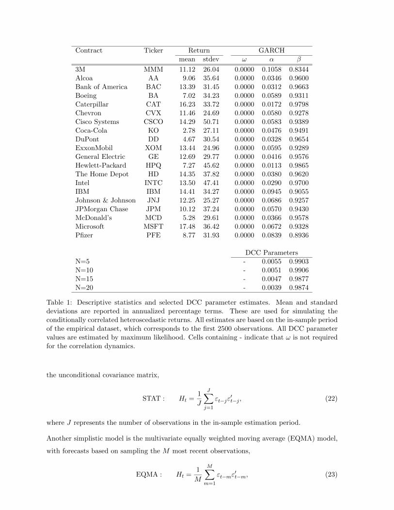
Contract Ticker Return GARCHmean stdev ω α β

3M MMM 11.12 26.04 0.0000 0.1058 0.8344Alcoa AA 9.06 35.64 0.0000 0.0346 0.9600Bank of America BAC 13.39 31.45 0.0000 0.0312 0.9663Boeing BA 7.02 34.23 0.0000 0.0589 0.9311Caterpillar CAT 16.23 33.72 0.0000 0.0172 0.9798Chevron CVX 11.46 24.69 0.0000 0.0580 0.9278Cisco Systems CSCO 14.29 50.71 0.0000 0.0583 0.9389Coca-Cola KO 2.78 27.11 0.0000 0.0476 0.9491DuPont DD 4.67 30.54 0.0000 0.0328 0.9654ExxonMobil XOM 13.44 24.96 0.0000 0.0595 0.9289General Electric GE 12.69 29.77 0.0000 0.0416 0.9576Hewlett-Packard HPQ 7.27 45.62 0.0000 0.0113 0.9865The Home Depot HD 14.35 37.82 0.0000 0.0380 0.9620Intel INTC 13.50 47.41 0.0000 0.0290 0.9700IBM IBM 14.41 34.27 0.0000 0.0945 0.9055Johnson & Johnson JNJ 12.25 25.27 0.0000 0.0686 0.9257JPMorgan Chase JPM 10.12 37.24 0.0000 0.0570 0.9430McDonald’s MCD 5.28 29.61 0.0000 0.0366 0.9578Microsoft MSFT 17.48 36.42 0.0000 0.0672 0.9328Pfizer PFE 8.77 31.93 0.0000 0.0839 0.8936

DCC ParametersN=5 - 0.0055 0.9903N=10 - 0.0051 0.9906N=15 - 0.0047 0.9877N=20 - 0.0039 0.9874

Table 1: Descriptive statistics and selected DCC parameter estimates. Mean and standarddeviations are reported in annualized percentage terms. These are used for simulating theconditionally correlated heteroscedastic returns. All estimates are based on the in-sample periodof the empirical dataset, which corresponds to the first 2500 observations. All DCC parametervalues are estimated by maximum likelihood. Cells containing - indicate that ω is not requiredfor the correlation dynamics.

the unconditional covariance matrix,

STAT : Ht =1

J

J∑j=1

εt−jε′t−j , (22)

where J represents the number of observations in the in-sample estimation period.

Another simplistic model is the multivariate equally weighted moving average (EQMA) model,

with forecasts based on sampling the M most recent observations,

EQMA : Ht =1

M

M∑m=1

εt−mε′t−m, (23)

10

with M = 100 used for this study.

The next model considered is the exponentially weighted moving average model (EWMA) in-

troduced by Riskmetrics (1996). Unlike the previous models that equally weight observations

within the sample period, the EWMA model applies a declining weighting scheme that places

greater weight on the most recent observation. This model takes the form,

EWMA : Ht = (1− λ) εt−1ε′t−1 + λHt−1, (24)

where λ is the parameter that controls the weighting scheme. Riskmetrics (1996) specify a

λ = 0.94 for data sampled at a daily frequency, the value used in this study.

The next model utilized is the exponentially weighted model of Fleming, Kirby and Ostdiek

(2001, 2003), denoted below as EXP,

EXP : Ht = α exp (−α) εt−1ε′t−1 + exp (−α)Ht−1, (25)

where α is the parameter that governs the weights on lagged observations. Similar to the

EWMA, a declining weighting scheme is applied to lagged observations, however this weighting

parameter is estimated by maximum likelihood.

The next three models are drawn from the conditional correlation multivariate GARCH class

of models. Along with the DCC model used as the DGP, the Constant Conditional Correlation

(CCC) model of Bollerslev (1990) and Asymmetric Dynamic Conditional Correlation (ADCC)

model of Cappiello, Engle and Sheppard (2006) are also used. The CCC model is recovered when

α and β in equation (21) are constrained to zero. The ADCC specification used here includes

asymmetric terms in both the conditional variance and correlation equations. Specifically, the

conditional variance equation follows that of Glosten, Jagannathan and Runkle (1993),

σ2i,t = $i + (αi + θiSi,t−1) ε2i,t−1 + βiσ

2i,t−1 , (26)

where θi captures the response of volatility to negative returns identified through the indicator

variable Si,t−1 that takes the value one if εi,t−1 < 0 and zero otherwise. The asymmetric

conditional correlation specification is

Qt = Q (1− α− β)− θm+ α(zt−1z

′t−1)

+ θmt−1m′t−1 + βQt−1 (27)

where θ is a asymmetric response parameter, mt−1 = δ � zt−1 is a dummy variable vector

with elements δi1 = 1 if zi,t−1 < 0 and m is the sample average of the outer products of mt.

Estimation of the conditional correlation models rely on the two stage maximum likelihood

procedure detailed by Engle and Sheppard (2001).

11

Finally, the Orthogonal GARCH (OGARCH) model of Alexander and Chibumba (1996) is also

considered. It reduces the dimensionality of the problem by creating orthogonal factors, fk,t,

through PCA. That is, the eigenvalues and eigenvectors of T−1∑T

t=1 z∗′t z∗t , where z∗t is the return

vector standardised by the unconditional standard deviation, are calculated. From these values

the N ×K matrix of standardised factor weights, W is formed, where its columns correspond

to eigenvectors of the K largest eigenvalues. The matrix of the orthogonal factors is formed as

ft = εtW. (28)

From this vector, the conditional variances are then estimated as

σ2k,t = ωk + αkf2l,t−1 + βkσk,t−1. (29)

Since the factors are orthogonal, the conditional covariance matrix of the factors, Vt, will have the

conditional variance of the factors on the main diagonal and zeros on all off-diagonal elements.

To obtain the conditional covariance matrix of the original return series the following calculation

is required to reverse the transformation and standardization that was performed,

OGARCH : Ht = AVtA′ =

K∑k=1

aka′kσ

2k,t (30)

where the elements of A are normalized factor weights, ak,i = wk,iσi. For this study, we set

K = N to ensure the invertibility of Ht, refer Bauwens et al. (2006).

One-step ahead volatility forecasts are then generated for each of these 700 observations using

each of the eight different forecasting methods. As mentioned earlier, the first 200 forecasts are

not used for forecast evaluations. Model parameters used for forecasting are those estimated

on the first 2500 observations from the empirical dataset and are not re-estimated at each

forecasting step. This implies that DCC model produces forecasts on the basis of the correct

DGP and all other forecasts originate from misspecified models. This setup was chosen in order

to focus upon the ability of the various evaluation techniques at identifying the best forecasting

model.

Finally, while MSE, MAE, QLK and MVPg loss functions rely only on the volatility forecast

and volatility proxy, MVP requires a target return, risk-free rate and a vector of expected

returns. Setting the target portfolio return is relatively easy under the given portfolio setting

and evaluation metric as all portfolios with target returns in excess of the risk-free rate have asset

weights that are purely scaled projections of each other. As such, the target return is set at 10%

p.a. The risk-free rate is set a constant 6% p.a., which is consistent with Fleming et al. (2001,

2003). Setting the vector of expected is not so simple as evaluations performed across different

12

vectors of expected returns are not guaranteed to produce the same conclusions. Fleming et al.

(2001, 2003), and Engle and Colacito (2006) outline approaches that address this issue in certain

settings, however, neither is tractable within this simulation environment. Therefore, to provide

insights into how the portfolio variance evaluations may vary across different assumed vectors

of expected returns, three vectors of expected return with varying quality are employed. The

first a constant mean, µ, which corresponds to the mean used to simulate returns, next a vector

containing the unconditional volatilities of the stock returns, σ, and finally a grid of values

[1, . . . , N ]′. Clearly the final two cases are incorrect, but these are chosen so as to highlight

any impact of assumptions regarding expected returns on model selection. To highlight which

vector of expected returns is used, MVP titles include the subscript µ, σ or 1, . . . , N .

5.3 Results

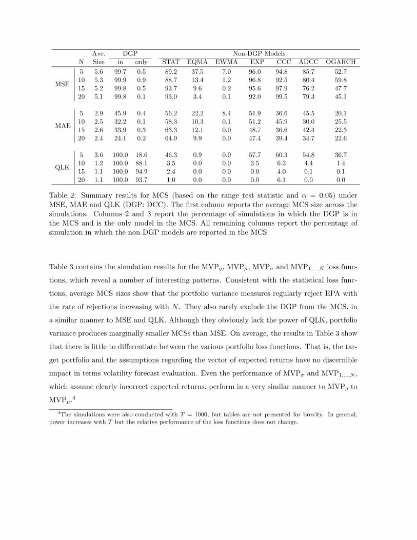
The performance of MSE, MAE and QLK are examined first and the results are presented in

Table 2. The first result column reports the average MCS size across the simulations. Reported

values indicate that each loss function generates EPA rejections, given the eight models in the

initial setM0. They also show that the ability to reject EPA within the MCS generally increases

as one moves from MSE to MAE and then to QLK. Moreover, for a given loss function, this

ability increases with N . In part, this increase in power potentially reflects an averaging of

losses over more elements and, or a deterioration in the performance in some of the models.

The second and third columns show that MSE almost always identifies the DGP as superior,

however, its lack of power means that it struggles to identify all inferior models. MAE rejects

EPA more frequently than MSE, but it is a poor substitute for MSE because it identifies the

DGP as inferior in the majority of simulations. Alternatively, QLK would be a good substitute.

It always identifies the DGP as superior and, especially at the higher dimensions, its ability

to identify inferior forecasting models is unequivocally superior to MSE and MAE. Finally, the

remaining columns report the frequency for which the non-DGP models appear in the MCSs.

Consistent with the average size findings reported in the second column, these frequencies

generally decrease as N increases. Some inconsistencies do arise, for example occurrences the

CCC model in the MCS increase when N increases from 15 to 20. This result reflects changes

in the relative performance of the competing models as the dimension grows. Overall these

results show that QLK outperforms MSE and MAE, and MAE is not a robust loss function for

multivariate volatility forecast evaluations. They are also consistent with the univariate results

of Patton (2011).

13

Ave. DGP Non-DGP ModelsN Size in only STAT EQMA EWMA EXP CCC ADCC OGARCH

MSE

5 5.6 99.7 0.5 89.2 37.5 7.0 96.0 94.8 85.7 52.710 5.3 99.9 0.9 88.7 13.4 1.2 96.8 92.5 80.4 59.815 5.2 99.8 0.5 93.7 9.6 0.2 95.6 97.9 76.2 47.720 5.1 99.8 0.1 93.0 3.4 0.1 92.0 99.5 79.3 45.1

MAE

5 2.9 45.9 0.4 56.2 22.2 8.4 51.9 36.6 45.5 20.110 2.5 32.2 0.1 58.3 10.3 0.1 51.2 45.9 30.0 25.515 2.6 33.9 0.3 63.3 12.1 0.0 48.7 36.6 42.4 22.320 2.4 24.1 0.2 64.9 9.9 0.0 47.4 39.4 34.7 22.6

QLK

5 3.6 100.0 18.6 46.3 0.9 0.0 57.7 60.3 54.8 36.710 1.2 100.0 88.1 3.5 0.0 0.0 3.5 6.3 4.4 1.415 1.1 100.0 94.9 2.4 0.0 0.0 0.0 4.0 0.1 0.120 1.1 100.0 93.7 1.0 0.0 0.0 0.0 6.1 0.0 0.0

Table 2: Summary results for MCS (based on the range test statistic and α = 0.05) underMSE, MAE and QLK (DGP: DCC). The first column reports the average MCS size across thesimulations. Columns 2 and 3 report the percentage of simulations in which the DGP is inthe MCS and is the only model in the MCS. All remaining columns report the percentage ofsimulation in which the non-DGP models are reported in the MCS.

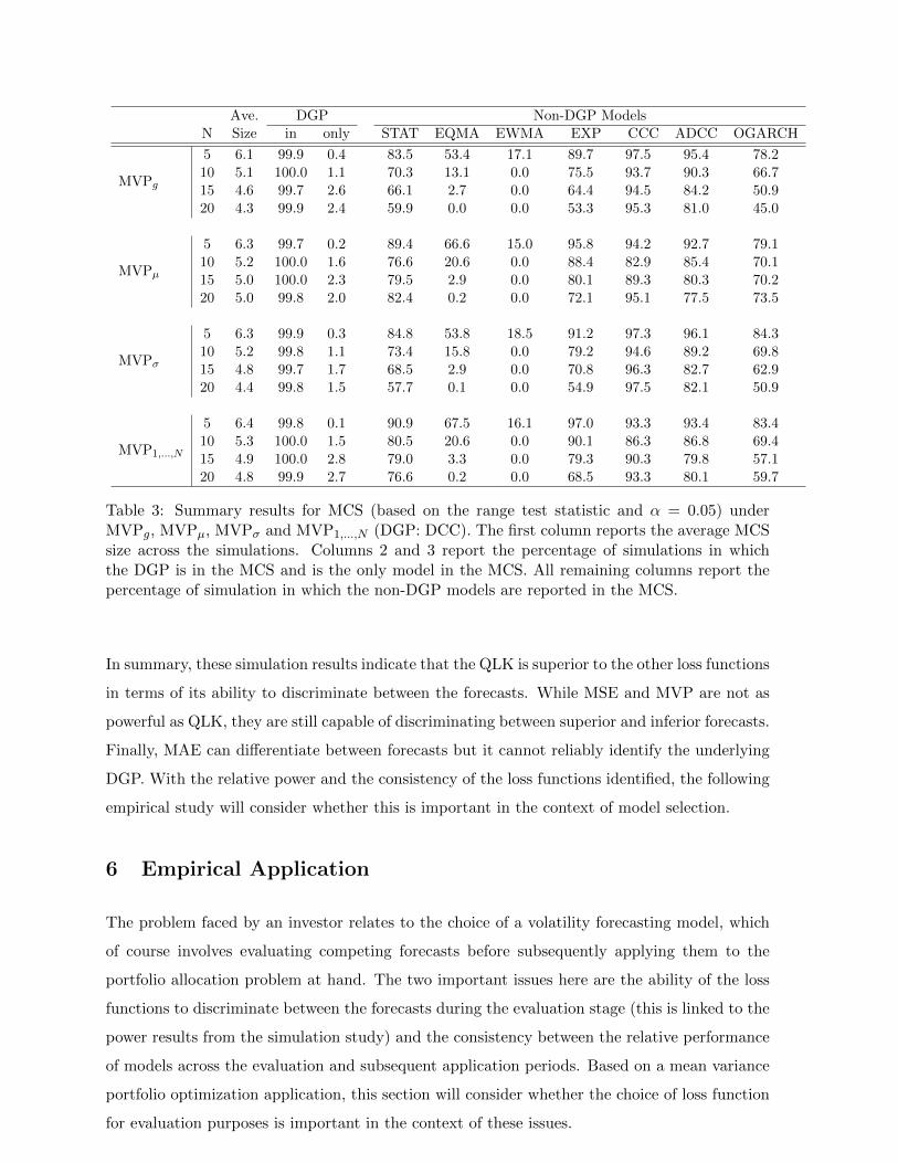
Table 3 contains the simulation results for the MVPg, MVPµ, MVPσ and MVP1,...,N loss func-

tions, which reveal a number of interesting patterns. Consistent with the statistical loss func-

tions, average MCS sizes show that the portfolio variance measures regularly reject EPA with

the rate of rejections increasing with N . They also rarely exclude the DGP from the MCS, in

a similar manner to MSE and QLK. Although they obviously lack the power of QLK, portfolio

variance produces marginally smaller MCSs than MSE. On average, the results in Table 3 show

that there is little to differentiate between the various portfolio loss functions. That is, the tar-

get portfolio and the assumptions regarding the vector of expected returns have no discernible

impact in terms volatility forecast evaluation. Even the performance of MVPσ and MVP1,...,N ,

which assume clearly incorrect expected returns, perform in a very similar manner to MVPg to

MVPµ.4

4The simulations were also conducted with T = 1000, but tables are not presented for brevity. In general,power increases with T but the relative performance of the loss functions does not change.

14

Ave. DGP Non-DGP ModelsN Size in only STAT EQMA EWMA EXP CCC ADCC OGARCH

MVPg

5 6.1 99.9 0.4 83.5 53.4 17.1 89.7 97.5 95.4 78.210 5.1 100.0 1.1 70.3 13.1 0.0 75.5 93.7 90.3 66.715 4.6 99.7 2.6 66.1 2.7 0.0 64.4 94.5 84.2 50.920 4.3 99.9 2.4 59.9 0.0 0.0 53.3 95.3 81.0 45.0

MVPµ

5 6.3 99.7 0.2 89.4 66.6 15.0 95.8 94.2 92.7 79.110 5.2 100.0 1.6 76.6 20.6 0.0 88.4 82.9 85.4 70.115 5.0 100.0 2.3 79.5 2.9 0.0 80.1 89.3 80.3 70.220 5.0 99.8 2.0 82.4 0.2 0.0 72.1 95.1 77.5 73.5

MVPσ

5 6.3 99.9 0.3 84.8 53.8 18.5 91.2 97.3 96.1 84.310 5.2 99.8 1.1 73.4 15.8 0.0 79.2 94.6 89.2 69.815 4.8 99.7 1.7 68.5 2.9 0.0 70.8 96.3 82.7 62.920 4.4 99.8 1.5 57.7 0.1 0.0 54.9 97.5 82.1 50.9

MVP1,...,N

5 6.4 99.8 0.1 90.9 67.5 16.1 97.0 93.3 93.4 83.410 5.3 100.0 1.5 80.5 20.6 0.0 90.1 86.3 86.8 69.415 4.9 100.0 2.8 79.0 3.3 0.0 79.3 90.3 79.8 57.120 4.8 99.9 2.7 76.6 0.2 0.0 68.5 93.3 80.1 59.7

Table 3: Summary results for MCS (based on the range test statistic and α = 0.05) underMVPg, MVPµ, MVPσ and MVP1,...,N (DGP: DCC). The first column reports the average MCSsize across the simulations. Columns 2 and 3 report the percentage of simulations in whichthe DGP is in the MCS and is the only model in the MCS. All remaining columns report thepercentage of simulation in which the non-DGP models are reported in the MCS.

In summary, these simulation results indicate that the QLK is superior to the other loss functions

in terms of its ability to discriminate between the forecasts. While MSE and MVP are not as

powerful as QLK, they are still capable of discriminating between superior and inferior forecasts.

Finally, MAE can differentiate between forecasts but it cannot reliably identify the underlying

DGP. With the relative power and the consistency of the loss functions identified, the following

empirical study will consider whether this is important in the context of model selection.

6 Empirical Application

The problem faced by an investor relates to the choice of a volatility forecasting model, which

of course involves evaluating competing forecasts before subsequently applying them to the

portfolio allocation problem at hand. The two important issues here are the ability of the loss

functions to discriminate between the forecasts during the evaluation stage (this is linked to the

power results from the simulation study) and the consistency between the relative performance

of models across the evaluation and subsequent application periods. Based on a mean variance

portfolio optimization application, this section will consider whether the choice of loss function

for evaluation purposes is important in the context of these issues.

15

The empirical study employs the eight volatility forecasting models described in Section 5. We

take an initial in-sample period of returns based on observations (t = 1, 2, ..., 2500) and for each

of the eight models, a one-step-ahead forecast H2501 is generated. Subsequent forecasts are then

generated by rolling the sample period of 2500 observations forward one observation until the

last forecast, H4000 is obtained, resulting in 1500 forecasts5. These 1500 forecasts are split into

three periods of 500 so as two sets of results may be presented. The first set of results are

based on evaluating the forecasts in the first period and applying them in the second period,

followed by results where the second and third periods are used for evaluation and application

respectively. The starting dates for the three periods of 500 forecasts are 5 December 2005, 20

November 2007 and 24 November 2009. The second period captures the onset of the financial

crisis in 2008 and is hence a period of much greater volatility than either the first or third

periods. The average annualized volatilities across the 20 stocks for each of the three periods

are 12.8%, 37.3% and 21.3%. Hence the conclusions drawn here are robust to the issue of

changes in market conditions between the periods when models are selected and subsequently

applied. All empirical analysis is conducted at dimensions of N = 5, 10, 15 and 20, where the

selected stocks at each dimension are defined earlier in the simulation study.

The competing forecasts are evaluated on the basis of MSE, MAE, QLK and portfolio variance.

For the statistical loss functions, the volatility proxy is either the outer-product of disturbances

generated under an AR(1) conditional mean process, or a realized estimate of the covariance

matrix based on intraday returns. Portfolio variance is measured for the global minimum vari-

ance and target return portfolios. Consistent with the simulation study, target return portfolios

are formed with µ0 = 10% and a risk-free rate of Rf = 6%. Three different vectors of expected

returns, they include: the mean from the first in-sample period, µ, the in-sample mean esti-

mated in the rolling window, µt, and an AR(1) mean, αrt−1. Subscripts are added to the MVP

titles to denote the results that relate to respective expected return assumptions.

The MCS framework will be used both in the evaluation and application periods to select the

superior set of forecasts that are of equal predictive accuracy given each of the loss functions.

The models contained in the MCS during the evaluation stage will be compared to those in

the MCS (given portfolio variance) in the application stage. Doing so, will shed light on the

consistency between the different loss functions and the final financial application in terms of

model selection and subsequent performance. The MCS results will be shown in a form where

a tick indicates that a particular forecast is contained within the MCS at α = 0.05.

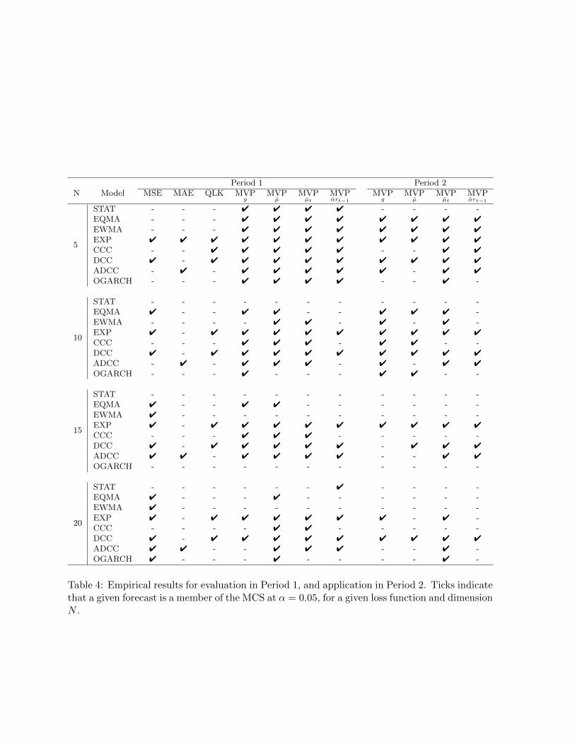
We begin by considering the results in Table 4 pertaining to forecast evaluation in Period 1, and

application in Period 2. MSE selects the EXP and DCC models at N = 5, but as N increases

5Parameters of the volatility models are only re-estimated at every 25th observation.

16

the number of models selected also increases, up to six at N = 20. MAE and QLK produce

smaller MCSs than MSE. Under MAE, the ADCC model is often the sole model reported in the

MCS. Given QLK, the MCS is marginally larger, identifying the EXP and DCC models as the

superior models. Unlike MSE, the performance of MAE and QLK does not appear to degrade

as N increases, both the size of the MCS and the set of superior forecasts remains quite stable.

Overall, these results are generally consistent with the simulation results in that MAE and

QLK produce smaller MCSs. In comparison, the portfolio variance based loss functions paint

a very different picture. The members of the MCS vary a great deal across both different N

and expected return assumptions. At N = 5, the MCS cannot not discriminate between any of

the forecasts, however as N increases, inferior forecasts begin to be identified. Once again, this

result is consistent with the simulation results in that MVP measures do not display the same

ability as either MAE or QLK. Interestingly, only QLK is consistent with the MVP measures

in terms of its MCS always being a subset of all MVP MCSs.

Now we turn to the consistency between the superior forecasts selected by the various loss func-

tions in the evaluation period, and the relative performance of the forecasts in the subsequent

application period (Period 2). While there is a degree of variation in the results, overall QLK

produces the best outcomes. It outperforms MVPg and MVP in that it leads to a smaller set

of superior models in the evaluation period, which are generally the better performing forecasts

in Period 2. For N = 5, QLK and MSE behave in a similar manner, however as N increases

the performance of MSE degrades as it often selects models not included in the Period 2 MCS.

QLK also outperforms MAE in that it always selects at least one model that is contained in the

Period 2 MCS. MAE does not display this quality. For example, at N = 20, QLK selects both

the EXP and DCC models, while MAE only selects the ADCC model. In Period 2, all four

MCSs contain the DCC model, as selected by QLK, but only one includes the ADCC model.

Therefore despite its ability to differentiate between models, in the evaluation period, MAE

is not selecting models that subsequently perform the best in the application period. While

both QLK and MAE can differentiate between forecasts, only QLK is consistent with the final

portfolio variance application.

We repeat the same process using Period 2 as for evaluation and Period 3 for the application of

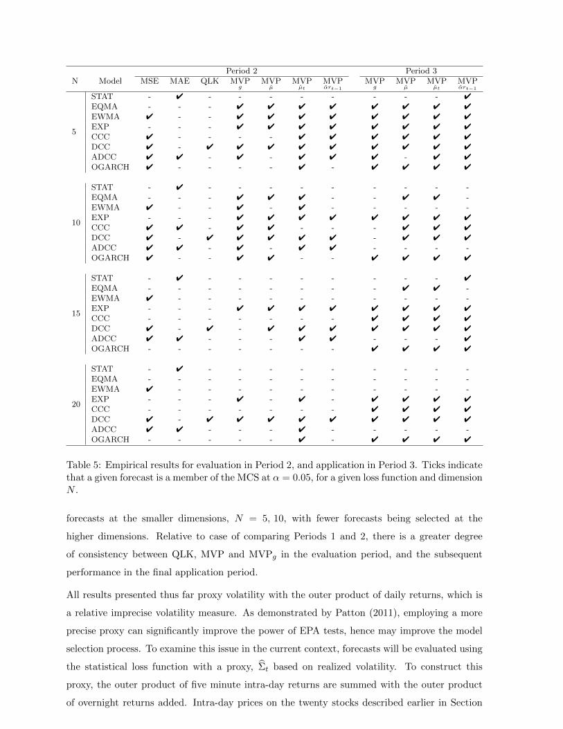
the forecasts, with results shown in Table 5. Overall, the results are similar to those discussed

above. Of the statistical loss functions, MSE leads to the largest MCSs, and is also inconsistent

with the application in it consistently excludes EXP but incorrectly includes EWMA and ADCC.

MAE also contradicts portfolio variance by including STAT, and excluding both the EXP and

DCC in Period 2. QLK continues to select models in a manner this is consistent with portfolio

variance. Once again, the MVPg and MVP loss function find it difficult to differentiate between

17

Period 1 Period 2N Model MSE MAE QLK MVP

gMVPµ

MVPµt

MVPαrt−1

MVPg

MVPµ

MVPµt

MVPαrt−1

5

STAT - - - 4 4 4 4 - - - -EQMA - - - 4 4 4 4 4 4 4 4

EWMA - - - 4 4 4 4 4 4 4 4

EXP 4 4 4 4 4 4 4 4 4 4 4

CCC - - 4 4 4 4 4 - - 4 4

DCC 4 - 4 4 4 4 4 4 4 4 4

ADCC - 4 - 4 4 4 4 4 - 4 4

OGARCH - - - 4 4 4 4 - - 4 -

10

STAT - - - - - - - - - - -EQMA 4 - - 4 4 - - 4 4 4 -EWMA - - - - 4 4 - 4 - 4 -EXP 4 - 4 4 4 4 4 4 4 4 4

CCC - - - 4 4 4 - 4 4 - -DCC 4 - 4 4 4 4 4 4 4 4 4

ADCC - 4 - 4 4 4 - 4 - 4 4

OGARCH - - - 4 - - - 4 4 - -

15

STAT - - - - - - - - - - -EQMA 4 - - 4 4 - - - - - -EWMA 4 - - - - - - - - - -EXP 4 - 4 4 4 4 4 4 4 4 4

CCC - - - 4 4 4 - - - - -DCC 4 - 4 4 4 4 4 - 4 4 4

ADCC 4 4 - 4 4 4 4 - - 4 4

OGARCH - - - - - - - - - - -

20

STAT - - - - - - 4 - - - -EQMA 4 - - - 4 - - - - - -EWMA 4 - - - - - - - - - -EXP 4 - 4 4 4 4 4 4 - 4 -CCC - - - - 4 4 - - - - -DCC 4 - 4 4 4 4 4 4 4 4 4

ADCC 4 4 - - 4 4 4 - - 4 -OGARCH 4 - - - 4 - - - - 4 -

Table 4: Empirical results for evaluation in Period 1, and application in Period 2. Ticks indicatethat a given forecast is a member of the MCS at α = 0.05, for a given loss function and dimensionN .

18

Period 2 Period 3N Model MSE MAE QLK MVP

gMVPµ

MVPµt

MVPαrt−1

MVPg

MVPµ

MVPµt

MVPαrt−1

5

STAT - 4 - - - - - - - - 4

EQMA - - - 4 4 4 4 4 4 4 4

EWMA 4 - - 4 4 4 4 4 4 4 4

EXP - - - 4 4 4 4 4 4 4 4

CCC 4 - - - - 4 4 4 4 4 4

DCC 4 - 4 4 4 4 4 4 4 4 4

ADCC 4 4 - 4 - 4 4 4 - 4 4

OGARCH 4 - - - - 4 - 4 4 4 4

10

STAT - 4 - - - - - - - - -EQMA - - - 4 4 4 - - 4 4 -EWMA 4 - - 4 - 4 - - - - -EXP - - - 4 4 4 4 4 4 4 4

CCC 4 4 - 4 4 - - - 4 4 4

DCC 4 - 4 4 4 4 4 - 4 4 4

ADCC 4 4 - 4 - 4 4 - - - -OGARCH 4 - - 4 4 - - 4 4 4 4

15

STAT - 4 - - - - - - - - 4

EQMA - - - - - - - - 4 4 -EWMA 4 - - - - - - - - - -EXP - - - 4 4 4 4 4 4 4 4

CCC - - - - - - - 4 4 4 4

DCC 4 - 4 - 4 4 4 4 4 4 4

ADCC 4 4 - - - 4 4 - - - 4

OGARCH - - - - - - - 4 4 4 4

20

STAT - 4 - - - - - - - - -EQMA - - - - - - - - - - -EWMA 4 - - - - - - - - - -EXP - - - 4 - 4 - 4 4 4 4

CCC - - - - - - - 4 4 4 4

DCC 4 - 4 4 4 4 4 4 4 4 4

ADCC 4 4 - - - 4 - - - - -OGARCH - - - - - 4 - 4 4 4 4

Table 5: Empirical results for evaluation in Period 2, and application in Period 3. Ticks indicatethat a given forecast is a member of the MCS at α = 0.05, for a given loss function and dimensionN .

forecasts at the smaller dimensions, N = 5, 10, with fewer forecasts being selected at the

higher dimensions. Relative to case of comparing Periods 1 and 2, there is a greater degree

of consistency between QLK, MVP and MVPg in the evaluation period, and the subsequent

performance in the final application period.

All results presented thus far proxy volatility with the outer product of daily returns, which is

a relative imprecise volatility measure. As demonstrated by Patton (2011), employing a more

precise proxy can significantly improve the power of EPA tests, hence may improve the model

selection process. To examine this issue in the current context, forecasts will be evaluated using

the statistical loss function with a proxy, Σt based on realized volatility. To construct this

proxy, the outer product of five minute intra-day returns are summed with the outer product

of overnight returns added. Intra-day prices on the twenty stocks described earlier in Section

19

Period 1 Period 2N Model MSE

RVMAERV

QLKRV

MVPg

MVPµ

MVPµt

MVPαrt−1

MVPg

MVPµ

MVPµt

MVPαrt−1

5

STAT - - - 4 4 4 4 - - - -EQMA - - - 4 4 4 4 4 4 4 4

EWMA - - - 4 4 4 4 4 4 4 4

EXP - 4 - 4 4 4 4 4 4 4 4

CCC - - 4 4 4 4 4 - - 4 4

DCC 4 - 4 4 4 4 4 4 4 4 4

ADCC - 4 - 4 4 4 4 4 - 4 4

OGARCH 4 - - 4 4 4 4 - - 4 -

10

STAT - - - - - - - - - - -EQMA - - - 4 4 - - 4 4 4 -EWMA 4 - - - 4 4 - 4 - 4 -EXP - - - 4 4 4 4 4 4 4 4

CCC - - 4 4 4 4 - 4 4 - -DCC 4 - 4 4 4 4 4 4 4 4 4

ADCC - 4 - 4 4 4 - 4 - 4 4

OGARCH 4 - - 4 - - - 4 4 - -

15

STAT - - - - - - - - - - -EQMA - - - 4 4 - - - - - -EWMA 4 - - - - - - - - - -EXP - - - 4 4 4 4 4 4 4 4

CCC - - - 4 4 4 - - - - -DCC 4 - 4 4 4 4 4 - 4 4 4

ADCC - 4 - 4 4 4 4 - - 4 4

OGARCH - - - - - - - - - - -

20

STAT - - - - - - 4 - - - -EQMA - - - - 4 - - - - - -EWMA 4 - - - - - - - - - -EXP - - - 4 4 4 4 4 - 4 -CCC - - - - 4 4 - - - - -DCC 4 - 4 4 4 4 4 4 4 4 4

ADCC - 4 - - 4 4 4 - - 4 -OGARCH 4 - - - 4 - - - - 4 -

Table 6: Empirical results for evaluation in Period 1, and application in Period 2. Ticks indicatethat a given forecast is a member of the MCS at α = 0.05, for a given loss function and dimensionN

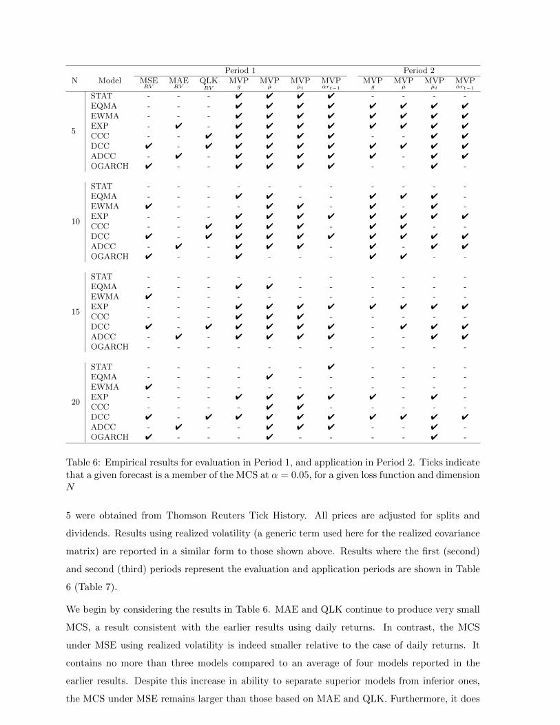
5 were obtained from Thomson Reuters Tick History. All prices are adjusted for splits and

dividends. Results using realized volatility (a generic term used here for the realized covariance

matrix) are reported in a similar form to those shown above. Results where the first (second)

and second (third) periods represent the evaluation and application periods are shown in Table

6 (Table 7).

We begin by considering the results in Table 6. MAE and QLK continue to produce very small

MCS, a result consistent with the earlier results using daily returns. In contrast, the MCS

under MSE using realized volatility is indeed smaller relative to the case of daily returns. It

contains no more than three models compared to an average of four models reported in the

earlier results. Despite this increase in ability to separate superior models from inferior ones,

the MCS under MSE remains larger than those based on MAE and QLK. Furthermore, it does

20

not generally select models in a manner consistent with portfolio variance. This is evident in

that its superior set of models often includes EWMA and OGARCH, which are often considered

inferior within the portfolio application. Therefore relative to the case of daily returns, the more

precise volatility proxy has improved the power of EPA tests within the MCS but this has not

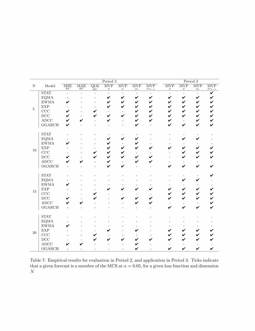
improved model selection for portfolio allocation purposes. Empirical results for evaluation in

Period 2 and application in Period 3 are reported in Table 7, and confirm the results from Table

6. The size of the MCS under MSE falls relative to the case of daily returns when the more

precise volatility proxy is employed. Despite this, it continues to select the inferior EWMA.

Results for MAE do not change, in that it continues to select a model that is inferior in the

subsequent application. Once again, QLK outperforms it counterparts by consistently selecting

models that are generally reported in the MCSs based on the applications. These results offer

additional support for the superiority of QLK and for model selection purposes.

Overall, these results support the use of QLK for model selection in the context of subsequent

application to a portfolio selection problem. QLK dominates the other loss function on the

grounds of both power in the evaluation period (consistent with the simulation findings) and

consistency with the final portfolio application. In the majority of instances, the models selected

by QLK are reported in subsequent portfolio based MCSs. MSE, MVPg and MVP lack the

power of QLK and result in larger MCSs in the evaluation period, often choosing models that

are inferior in the subsequent application. While MAE displayed considerable power in the

evaluation period, it often selects models that were inferior in the subsequent application. The

use of realized volatility improved the power of the statistical loss functions in the evaluation

period, a result consistent many studies involving the measurement, and forecasting of volatility.

However this additional power did not translate into improved model selection.

7 Conclusion

While techniques for evaluating univariate volatility forecasts are well understood, the literature

relating to multivariate volatility forecasts is less developed. Many financial applications employ

multivariate volatility forecasts, thus it may be appealing evaluate and select forecasts model on

the basis of such an application. In this paper we investigate the performance of a range of loss

functions for selecting models to be applied in a subsequent portfolio allocation problem. Two

issues underly this problem, the relative power of the loss functions, and the consistency with the

final portfolio application. Simulation results demonstrate that a statistical loss function based

on the multivariate normal likelihood (QLK) has more power than any other loss function

considered. This translates into the empirical setting where QLK identifies a small number

of models during the evaluation period, most of which produce superior portfolio outcomes

21

Period 2 Period 3N Model MSE

RVMAERV

QLKRV

MVPg

MVPµ

MVPµt

MVPαrt−1

MVPg

MVPµ

MVPµt

MVPαrt−1

5

STAT - - - - - - - - - - 4

EQMA - - - 4 4 4 4 4 4 4 4

EWMA 4 - - 4 4 4 4 4 4 4 4

EXP - - - 4 4 4 4 4 4 4 4

CCC 4 - 4 - - 4 4 4 4 4 4

DCC 4 - 4 4 4 4 4 4 4 4 4

ADCC 4 4 - 4 - 4 4 4 - 4 4

OGARCH 4 - - - - 4 - 4 4 4 4

10

STAT - - - - - - - - - - -EQMA - - - 4 4 4 - - 4 4 -EWMA 4 - - 4 - 4 - - - - -EXP - - - 4 4 4 4 4 4 4 4

CCC - - 4 4 4 - - - 4 4 4

DCC 4 - 4 4 4 4 4 - 4 4 4

ADCC 4 4 - 4 - 4 4 - - - -OGARCH - - - 4 4 - - 4 4 4 4

15

STAT - - - - - - - - - - 4

EQMA - - - - - - - - 4 4 -EWMA 4 - - - - - - - - - -EXP - - - 4 4 4 4 4 4 4 4

CCC - - 4 - - - - 4 4 4 4

DCC 4 - 4 - 4 4 4 4 4 4 4

ADCC 4 4 - - - 4 4 - - - 4

OGARCH - - - - - - - 4 4 4 4

20

STAT - - - - - - - - - - -EQMA - - - - - - - - - - -EWMA 4 - - - - - - - - - -EXP - - - 4 - 4 - 4 4 4 4

CCC - - 4 - - - - 4 4 4 4

DCC - - 4 4 4 4 4 4 4 4 4

ADCC 4 4 - - - 4 - - - - -OGARCH - - - - - 4 - 4 4 4 4

Table 7: Empirical results for evaluation in Period 2, and application in Period 3. Ticks indicatethat a given forecast is a member of the MCS at α = 0.05, for a given loss function and dimensionN

22

in subsequent application period. Portfolio variance does not display the same quality, models

deemed superior in one period are often found to be inferior in the next. We have also considered

the effect of different volatility proxies. Our empirical results relating the selection of models

remain constant when either the outer product of daily returns or a realized volatility proxy

volatility are used for evaluation purposes. Overall, these findings extend our understanding of

the evaluation of multivariate volatility forecasts and provide guidance for practitioners when

selecting models for the purposes of portfolio construction.

23

References

Alexander, C. and Chibumba, A. (1996), ”Multivariate orthogonal factor GARCH” Working

Paper, Sussex, University of Sussex.

Amenc N., Goltz F., Tang L. and Vaidyanathan V. (2012), EDHEC-Risk North American

Index Survey 2011, EDHEC-Risk Institute Publication, April 2012.

Andersen T.G., Bollerslev T., Diebold F.X. and Labys P. (2003), ”‘Modeling and forecasting

realized volatility”’. Econometrica, 71, 579-625.

Andersen, T.G., Bollerslev, T., Christoffersen, P.F. and Diebold, F.X. (2006), Volatility and

Correlation Forecasting, in Handbook of Economic Forecasting, eds. Elliot, G., Granger, C.W.J.

and Timmerman, A., Elsevier, Burlington.

Bauwens, L., Laurent, S. and Rombouts, V. K. (2006), ”‘Multivariate GARCH models: a

review” Journal of Applied Econometrics, 21, 79-109.

Becker, R., and Clements, A. (2008), ”Are combination forecasts of S&P 500 volatility statis-

tically superior?”, The International Journal of Forecasting, 24, 122-133.

Bollerslev, T. (1990), ”Modelling the coherence in short-run nominal exchange rates: A mul-

tivariate generalized ARCH model”, Review of Economics and Statistics, 72, 498-505.

Cappiello, L., Engle, R.F. and Sheppard, K. (2004), ”Asymmetric dynamics in the correlations

of global equity and bond returns”, Journal of Financial Econometrics, 4, 537-572.

Caporin, M., and McAleer, M. (2010), ”Ranking multivariate GARCH models by problem

dimension” Working Paper, Padova, University of Padova.

Campbell, J.Y., Lo, A.W. and MacKinlay, A.G. (1997), The Econometrics of Financial Mar-

kets, Princeton University Press, Princeton NJ.

Danielsson, J. (2011), Financial Risk Forecasting, John Wiley & Sons Ltd., Chichester.

Diebold, F.X. and Mariano, R.S. (1995), ”Comparing predictive accuracy”, Journal of Business

and Economics Statistics, 13, 253-263.

Elliott, G. and Timmermann, A. (2008), ”Economic Forecasting”, Journal of Economic Liter-

ature, textbf46, 3-56.

Engle, R.F. (1982), ”Autoregressive conditional heteroscedasticity with estimates of the vari-

ance of United Kingdom inflation”, Econometrica, 50, 987-1007.

24

Engle, R.F. (2002), ”Dynamic conditional correlation: a simple class of multivariate general-

ized autoregressive conditional heteroskedasticity models”, Journal of Business and Economic

Statistics, 20, 339-350.

Engle, R. and Colacito, R. (2006), ”Testing and valuing dynamic correlations for asset alloca-

tion”, Journal of Business and Economic Statistics, 24, 238-253.

Engle, R. F. and Sheppard, K. (2001), ”Theoretical and empirical properties of dynamic condi-

tional correlation multivariate GARCH”, Working Paper, University of California San Diego.

Fleming, J., C. Kirby and B. Ostdiek. (2001), ”The economic value of volatility timing”, The

Journal of Finance, 56, 329-352.

Fleming, J., C. Kirby and B. Ostdiek. (2003). ”The economic value of volatility timing using

realized volatility”, Journal of Financial Economics, 67, 473-509.

Glosten, L.R., Jagannathan, R. and Runkle, D.E. (1993). ”On the relation between the ex-

pected value and the volatility of the nominal excess return on stocks”, Journal of Finance,

48, 1779-1801.

Gourieroux, C. and Jasiak, J. (2001), Financial Econometrics. Princeton University Press,

Princeton NJ.

Hansen, P. (2005), ”A test for superior predictive ability”, Journal of Business and Economic

Statistics, 23, 365-380.

Hansen, P. and Lunde A. (2006), “Consistent ranking of volatility models”, Journal of Econo-

metrics, 131, 97-121.

Hansen, P., Lunde, A. and Nason, J. (2003), ”Choosing the best volatility models: the model

confidence set approach”, Oxford Bulletin of Economics and Statistics, 65, 839-861.

Hansen, P., Lunde, A. and Nason, J. (2011), ”The model confidence set”, Econometrica, 79,

453-497.

Laurent, S., Rombouts, G. and Violante, F. (2009), ”On loss functions and ranking forecasting

performance of multivariate volatility models”, Working Paper, CIRPEE.

Laurent, S., Rombouts, G. and Violante, F. (2010), ”On the forecasting accuracy of multivari-

ate GARCH models”, Working Paper, CIRPEE.

Patton, A. (2011), ”Volatility forecast comparison using imperfect volatility proxies”, Journal

of Econometrics, 161, 284-303.

25

Patton, A. and Sheppard, K. (2009), Evaluating Volatility Forecasts, in Handbook of Financial

Time Series, Andersen, T.G., Davis, R.A., Kreiss, J.P. and Mikosch, T. eds., Springer-Verlag.

Poon, S-H. and Granger, C.W.J. (2003), ”Forecasting volatility in financial markets: a review”,

Journal of Economic Literature, 41, 478-539.

Poon, S-H. and Granger, C.W.J. (2005), ”Practical Issues in forecasting volatility”, Financial

Analysts Journal, 61, 45-56.

Riskmetrics. (1996), Technical Document, New York, JP Morgan/Reuters.

Silvennoinen, A. and Terasvirta, T., (2009), ‘Multivariate GARCH models in Handbook of Fi-

nancial Time Series, Andersen, T.G., Davis, R.A., Kreiss, J.P. and Mikosch, T. eds., Springer-

Verlag.

West, K.D. (1996), ”Asymptotic inference about predictive ability”, Econometrica, 64, 1067-

1084.

West, K.D., Edison, H.J. and Cho, D. (1993), “A utility-based comparison of some models of

exchange rate volatility ”, Journal of International Economics, 35, 23-45.

White, H. (2000), ”A reality check for data snooping”, Econometrica, 68, 1097-1125.

26