Coordinating Supply Chains with Competition: Capacity Allocation in Semiconductor Manufacturing

Suman Mallik Patrick T. Harker mallik@uiuc.edu harker@wharton.upenn.edu Department of Business Administration Operations and Information Management University of Illinois The Wharton School 350 Commerce West, 1206 S. Sixth Street University of Pennsylvania Champaign, IL 61820 Philadelphia, PA 19104-6366

February 1999

Revised July 2000

Abstract

This paper, motivated by the experiences of a major US-based semiconductor manufacturer, presents an integrated model of incentive problems arising in forecasting and capacity allocation. Our model involves multiple product managers and multiple manufacturing managers who forecast the means of their respective demand and capacity distributions. A central coordinator is responsible for allocating capacities to product lines. When these distributions are unknown to the central coordinator and capacity is scarce, the managers misrepresent their forecasts. A product manager inflates his forecast to gain a greater allocation of the capacity; a manufacturing manager deflates his forecast to cover for the uncertainties in production. We propose a game theoretic model and design a mechanism (a bonus scheme for all managers and an allocation rule to allocate realized capacity to the product managers) that elicits truthful reporting by all managers. The results herein show that the structure of the optimal bonus schemes is rather simple with easily calculable parameters. We also show that large classes of allocation rules, including the current practice of proportional allocation by the firm, are manipulable. A bonus is often required for elicitation of truthful information. We synthesize the implications of our results for the practitioners. Keywords: coordination, supply chain management, demand forecasting, game theory, capacity allocations, incentives, mechanism design

2

1.0 INTRODUCTION

This paper presents an integrated model of the incentive problems arising in demand

forecasting and capacity allocation within a multi-divisional/multi plant firm. The research is

motivated by the experiences of a major US-based semiconductor manufacturer. The firm is in

the business of manufacturing and marketing of telecommunications, electronic, and computer

equipment. A large proportion of its product mix consists of relatively short life cycle (about 2

years) products. Moreover, a semiconductor chip loses 60% of its value within first six or seven

months of its life cycle. The firm operates five semiconductor fabrication facilities (fabs), each

of which produces multiple products (there are 36 different product lines). Each fab is headed by

a manufacturing manager (MM) while each product group is headed by a product manager (PM).

The operating environment is characterized by volatile demand and high manufacturing lead-

times (about 2-3 months), which require that the production and capacity allocation decisions be

made before the demand is known. Thus, the firm allocates the available capacities to competing

product lines based on forecasts. The dynamics of this process is as follows:

• At the beginning of every month, a PM gives the quarterly demand forecasts of his product

for the current quarter and for the remaining quarters of the current year to the central

coordinator. These forecasts are point forecasts of the average of the random demands.

• At the beginning of a year, a MM submits forecasts of available capacities for the current

year to the central coordinator. The forecast of a MM is also a point forecast of the average

of the random capacity. The capacity, in our context, is treated as a random variable because

the yield in semiconductor manufacturing is random. The overall yield is actually a

combination of two yields: the line yield and the die yield. While the line yield can be

controlled with managerial effort, the die yield is extremely difficult to control. This is the

main reason behind treating capacities as random variables.

• Based on the forecasts, the center allocates the capacities to the different products for the

planning year. Thus, capacity allocation decisions are made only once every year. We note

that there is no formal method of capacity allocation at the said firm. Personal clouts of the

3

individual managers play a major role in capacity allocation! However, the allocation

process had some crude similarities with proportional allocation.

The coordination process is characterized by information asymmetry, which leads to

misrepresentation of forecasts. The product managers and the manufacturing managers possess

private information about the respective demands and capacities. In the presence of capacity

shortages (which are always the case for the firm under consideration), a PM has an incentive to

inflate his forecast to get a greater allocation of the capacity. On the other hand, a MM tends to

understate the capacity of a plant to cover for the uncertainties. The objective of this study is to

design a mechanism that will induce truthful reporting by the managers. By the term mechanism

we mean an allocation rule for the PMs that the center follows to allocate capacities to different

products, and a bonus scheme for all managers. In particular, we address the following issues.

• What are the structures of the bonus schemes under different conditions of information

availability? Are the bonuses always required?

• What kinds of allocation rules are truthful under different conditions of information

availability?

Coordination and contracting have been studied extensively under different contexts in the

operations management literature. A few recent examples are Cachon & Leriviere (1999 a, b),

Corbett (1996), Hauser et al. (1994), Grout and Christy (1993), and Porteus and Whang (1991).

The majority of these works, like the principal-agent models of economics, consider the

contracting problem between two individuals. Porteus & Whang (1991) and Cachon & Leriviere

(1999a, b) consider the contracting problem between one supplier and multiple retailers. Our

work is a generalization of these works in the sense that we consider the contracting problem

between two groups of individuals. Thus, our problem contains a market-like structure between

suppliers and retailers.

The remainder of the paper is organized as follows. The next section reviews the

appropriate literature and positions our work with respect to this literature. In Section 3, we

present a formal game theoretic model that specifically captures the information asymmetry and

divergence of preferences of the managers and derive insights from it. Implications for the

4

practitioners are summarized in Section 4. We end with summary and directions for future

research in Section 5.

2.0 LITERATURE REVIEW

The incentive issues in intra-firm coordination and supply chain management have been

addressed in literature in many different forms and contexts. We provide a brief description of

the papers that relate closely to our work. The reader is referred to the work of Tsay Nahmias,

and Agrawal (1999) for a comprehensive review of contracting literature in supply chain

management. Whang (1995) provides for a formal classification of coordination problems in

operations management.

The stochastic multi-echelon inventory theory literature generally assumes the existence

of a central planner with full information of the system and with the power to implement a

centrally optimal solution on the entire system. The supply chain contracting literature usually

relaxes these assumptions. Axsater (1993) provides for an excellent summary of stochastic

multi-echelon inventory theory literature. Clark & Scarf (1960), one of the classic papers in the

field, show that finding optimal policies for a multi-echelon system can be reduced to finding

optimal policies for each echelon individually by imposing an appropriate cost structure. Lee &

Whang (1994) build on this idea to develop an incentive system that will induce the individual

echelon managers to take jointly optimal decisions using locally available information and

leaving them at least as well off as they would be under the Clark & Scarf (1960) scheme.

Porteus & Whang (1991) studied a coordination problem between one manufacturing

manager and several product managers. The product managers make sales efforts while the

manufacturing manager makes efforts for capacity realization and decides inventory levels for

different products. They seek incentive plans that will induce the managers to act in such a way

that owner of the firm can attain maximum possible returns. Grout & Christy (1993) let a buyer

give the supplier a bonus for on-time delivery, making the supplier take the buyer’s stockout cost

into account when determining his stock level. Corbett (1996) considered the case of one

supplier and one customer where the supplier holds inventory at the customer’s premises and the

customer has private information about his stockout costs. Cachon & Lariviere (1999b) consider

5

the problem of capacity allocation problem of a manufacturer faced with demands from multiple

retailers each having private information. They present allocation mechanisms under which truth

telling is an equilibrium strategy and conclude that truth telling can lower the profit of the

supplier, the supply chain and even the retailers. Cachon & Lariviere (1999a) propose a two-

period game to model the turn-and-earn allocation observed in automotive industry.

All of the works described in this section consider one manufacturing manager/supplier

and multiple customers. In particular, the works by Hauser et al. (1994) and Corbett (1996)

involve only one supplier and one customer. In contrast, we consider multiple manufacturing

managers (suppliers) along with multiple product managers (customers). Our problem, thus,

contains a market-like structure that allows us to study the strategic interactions not only between

the product managers but also between the manufacturing managers.

3.0 THE MODEL

Our analysis concerns the simplest model that contains the essential features of capacity

allocation at the semiconductor manufacturer described in Section 2. In line with our observation

at the firm, our model assumes the existence of a capacity shortage. Thus, we consider allocation

of capacity to the products and not the opposite scenario. Section 3.1 gives the model

specification, relevant analyses are presented in Section 3.2.

3.1 Model Specification

The players in our model are the individual managers (i.e., the PMs and the MMs). The

respective strategies are the reports of the means of the respective distributions. The strategies

belong to a strategy set defined by the support of the respective distributions. The following

subsections formally define the model.

3.1.1 Assumptions

The following assumptions will be used throughout the remainder of the paper:

6

1. Single period model with no inventory carryover. We mentioned in Section 1 that allocation

of capacity was done only once a year. Typical product life cycle in semiconductor

manufacturing is 12-18 months. Thus, single period is a reasonable assumption.

2. The center as well as all managers is risk neutral. This assumption is often made in

operations management literature.

3. Demands are independent of each other. This assumption is required for analytical

tractability. This is a reasonable assumption given the large number of products and large

number of suppliers (of the each product) in semiconductor industry.

4. Capacity of each plant is independent of the others. The capacities are independent of the

demands.

5. Problem parameters (holding, penalty and shortage costs, product revenues etc.) are common

knowledge. This is a valid assumption as all managers are part of the same firm. There is

very little uncertainty regarding the accounting procedures and parameters.

6. All managers are treated equally in the allocation process; i.e., personal clout of the managers

does not influence the allocation decisions.

3.1.2 The Timing

The timing of the events is as follows:

1. The managers privately learn the distribution of their respective demands or capacities.

2. The center announces the allocation rule for the product managers and the incentive schemes

for both the product and manufacturing managers for all possible realizations of demands and

capacities. All managers observe the announcement.

3. The PMs and MMs give their forecasts to the center. Others do not observe the forecast of a

manager.

4. Production takes place. Capacities are realized, and are seen by all.

5. Allocations are made by the center and are observed by all parties.

6. Demand is realized and is seen by all. The managers are rewarded as per announced

incentive schemes.

7

We mentioned in Section 1 that capacity allocation is done only once a year. Manufacturing

starts out with a tentative schedule based on the forecast of the MMs. As the time evolves, the

random capacities are realized. The central coordinator often revises production plans during the

year in response to the realizations of capacities. This explains the rational behind doing the

allocation after the realization of capacities in our model.

Lastly, it is important to note that the firm uses a set of normalization factors to determine

capacity consumed by different products. For example, capacity consumed by 1 unit of

1.25µ/1.75µ CMOS is equivalent to capacity consumed by 1.4 units of 0.3µ/0.35µ LIN at a

particular fab. Thus, there is a one to one correspondence between capacity consumed by each

product at any specific manufacturing plant.

3.1.3 Notation

We define the following quantities:

i = index on product, i = 1, 2, …, n,

k = index on plant, k = 1, 2, …, m,

hi = unit overage cost of product i,

pi = unit shortage cost for product i,

ei = unit revenue for product i,

Zi = random demand for product i, with distribution function Gi(.), density gi(.)

and mean νi; zi is a realization of Zi,

αi = demand forecast of product i,

Bk = random capacity for plant k, with distribution function Fk(.), density fk(.) and

mean µk; bk is a realization of Bk,

βk = capacity forecast of plant k,

),( kk BS β = bonus for MM k,

),( ii Zr α = bonus for PM i.

Let β = (β1, β2, …βm) be the m-vector of reported capacities and α = (α1, α2, …, αn) be the n-

vector of reported demands. Let β-k denote the m-1 vector (β1, β2, …, βk-1, βk+1, …, βm), and α-i

8

denote the n-1 vector (α1, α2, …, αi-1, αi+1, …,αn). Therefore, α = (αi, α-i) and β = (βk, β-k).

Finally, let (x)+ denote max{x,0}.

3.1.4 Utility Maximization Problems

Problem faced by Manufacturing Manager k, k = 1, 2, ..., m

The payoff of MM k is his bonus S bk k( , )β . Under the assumption of risk neutrality, the

problem faced by the MM is given by

Max E S Bk

kF k kββ( , ) . (1)

The bonus, Sk(β, Bk), is a function of the reported capacities of all MMs as well as that of the

realized capacity of MM k. Note that this formulation allows us to capture the strategic

interactions between the manufacturing managers. A manufacturing manager knows that today’s

forecast is tomorrow’s production quota. Therefore, to cover for the uncertainties in the

production process, he tends to understate his capacity.

Problem Faced by Product Manager i, i = 1, 2, ..., n

The payoff of PM i, R zi i( , )α , is the sum of two components: the bonus payment ri(.)

received for participating in the forecasting process; and a pre-specified fraction, iψ , of the profit

(.)iπ arising from selling the product to the customer. Thus,

),(),z),(()z,(r)z,(R iiiiiiiii 10∈+= ψαπψαα λ , (2)

where λi ( )α is the allocation rule and denotes the allocation received by product manager i,

given the vector of reported forecasts α . This allocation rule is announced by the center before

the managers give the forecasts. Cachon & Lariviere (1999b) described different properties of

traditional allocation rules. Under an individually responsive (IR) allocation mechanism, if one

is receiving a positive allocation but wants more, one gets more unless one has already claimed

all of capacity. The examples are proportional allocation, linear allocation etc. We consider a

newsboy type profit function for each product manager i, i = 1, 2, ..., n. Thus,

++ α−−−α−α=απ )](Z[p]Z)([h}Z),(min{e)Z),(( iiiiiiiiiiii λλλλ . (3)

9

In (3) we have, without loss of generality, normalized the variable cost of production to zero.

Note that we consider iψ ’s to be given. The utility maximization problem faced by the PM,

under the assumption of risk neutrality, is given by:

Max E R Zi

iG i iαα( , ) . (4)

Problem of the Central Coordinator

The aim of the central coordinator is to design a mechanism such that it induces truthful

reporting by all managers. By the word mechanism we mean the allocation rule λi ( )α for the

product managers and the bonus schemes (or the incentive schemes), S bk k( , )β and r zi i( , )α .

Thus, the problem of the center is to choose λi ( )α , r zi i( , )α , and S bk k( , )β such that truth-

telling is equilibrium strategy of each manager. Note that we did not specify the issue of

optimality of allocation while specifying the objective of the central coordinator. We mentioned

in earlier that the firm currently does not take into account the differential product margins while

doing the allocation. In line with this observation, seeking optimal allocation is one objective of

this paper, though not the sole objective. Thus, we seek to specify which allocation rule and

bonus schemes are truthful. Within this broad framework of truth-telling, we also seek to study

the feasibility of implementing an optimal allocation by revelation. We call this as the optimal

forecast design problem or simply the optimal allocation problem.

The Optimal Allocation Problem

An optimal allocation maximizes the total profit of the firm less the incentive payments.

The following is a formulation of the optimal allocation problem.

})B,(S)Z,(r)Z),(()({Emaxm

kkk

n

iii

n

iiiiiS,r, kii

∑∑∑===

−−−111

1 βααπψ λλ

(5)

Subject to

βαα ∀∀≤∑=

,;)(1

Kn

iiλ , (6)

10

where K is the total realized capacity. Under the assumption that the revelation principle holds,

the central coordinator can restrict itself to searching for only those mechanisms under which

each manager reveals their respective private information truthfully. Thus, we have:

);,(maxarg iiiiGi ZREi

i

−′

′= αανα

, (7)

);,(maxarg kkkkFk BSEk

k

−′

′= ββµβ

, (8)

.)(,(.)r,(.)S iik 000 ≥≥≥ αλ . (9)

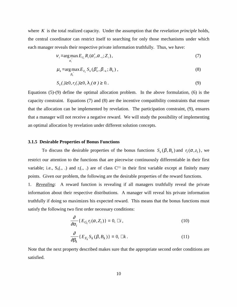
Equations (5)-(9) define the optimal allocation problem. In the above formulation, (6) is the

capacity constraint. Equations (7) and (8) are the incentive compatibility constraints that ensure

that the allocation can be implemented by revelation. The participation constraint, (9), ensures

that a manager will not receive a negative reward. We will study the possibility of implementing

an optimal allocation by revelation under different solution concepts.

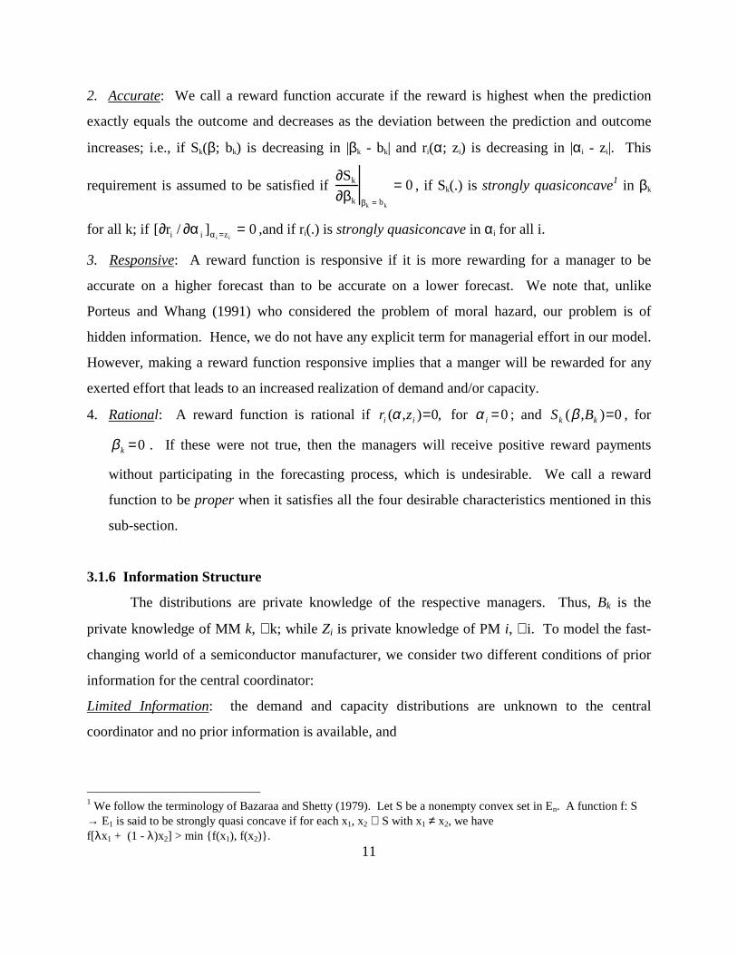
3.1.5 Desirable Properties of Bonus Functions

To discuss the desirable properties of the bonus functions ),( kk BS β and r zi i( , )α , we

restrict our attention to the functions that are piecewise continuously differentiable in their first

variable; i.e., Sk(., .) and ri(., .) are of class C(1) in their first variable except at finitely many

points. Given our problem, the following are the desirable properties of the reward functions.

1. Revealing: A reward function is revealing if all managers truthfully reveal the private

information about their respective distributions. A manager will reveal his private information

truthfully if doing so maximizes his expected reward. This means that the bonus functions must

satisfy the following two first order necessary conditions:

∂∂α

αi

G i iE r Z ii

{ ( , )} ,= ∀0 , (10)

∂∂β

βk

F k kE S B kk

{ ( , )} ,= ∀0 . (11)

Note that the next property described makes sure that the appropriate second order conditions are

satisfied.

11

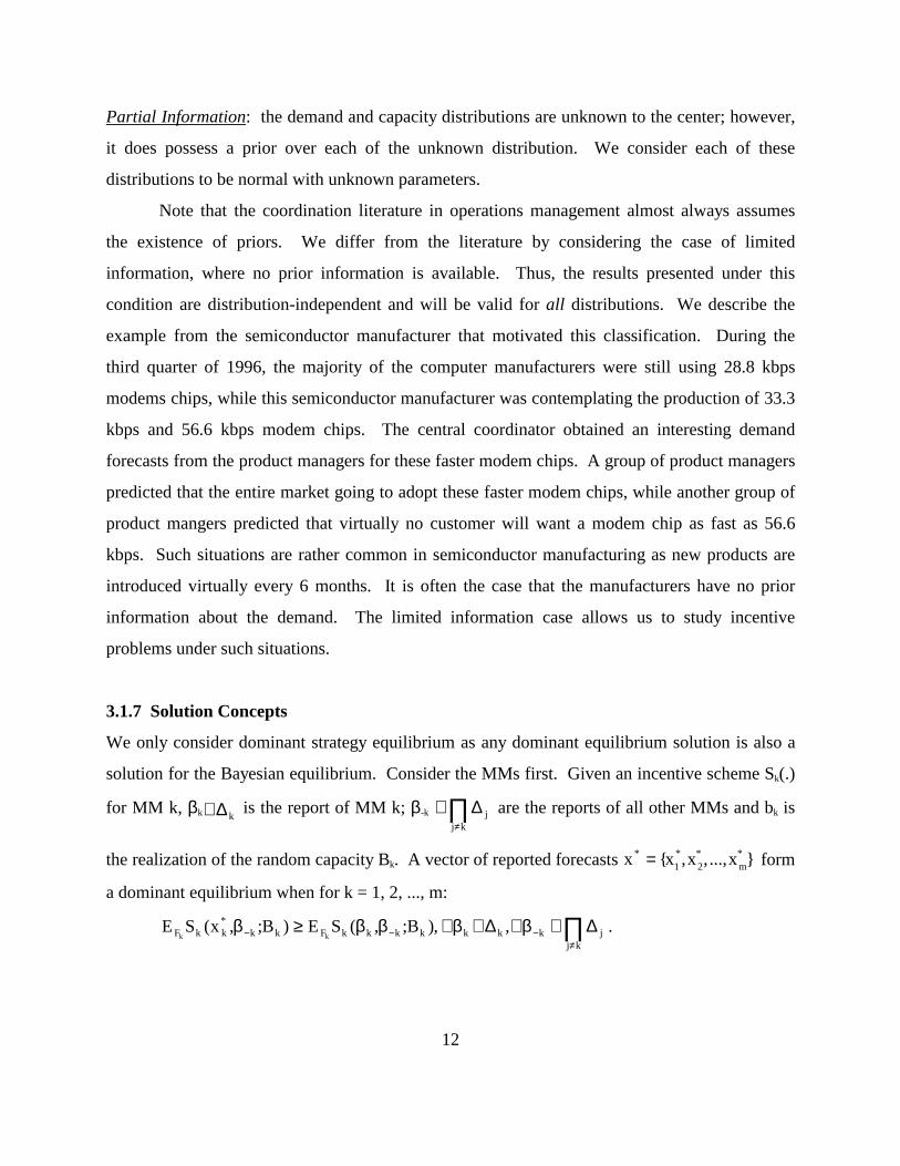
2. Accurate: We call a reward function accurate if the reward is highest when the prediction

exactly equals the outcome and decreases as the deviation between the prediction and outcome

increases; i.e., if Sk(β; bk) is decreasing in |βk - bk| and ri(α; zi) is decreasing in |αi - zi|. This

requirement is assumed to be satisfied if ∂Sk

∂βk βk = bk

= 0 , if Sk(.) is strongly quasiconcave1 in βk

for all k; if 0]/r[ii zii =α∂∂ =α ,and if ri(.) is strongly quasiconcave in αi for all i.

3. Responsive: A reward function is responsive if it is more rewarding for a manager to be

accurate on a higher forecast than to be accurate on a lower forecast. We note that, unlike

Porteus and Whang (1991) who considered the problem of moral hazard, our problem is of

hidden information. Hence, we do not have any explicit term for managerial effort in our model.

However, making a reward function responsive implies that a manger will be rewarded for any

exerted effort that leads to an increased realization of demand and/or capacity.

4. Rational: A reward function is rational if ,0),( =ii zr α for 0=iα ; and 0),( =kk BS β , for

0=kβ . If these were not true, then the managers will receive positive reward payments

without participating in the forecasting process, which is undesirable. We call a reward

function to be proper when it satisfies all the four desirable characteristics mentioned in this

sub-section.

3.1.6 Information Structure

The distributions are private knowledge of the respective managers. Thus, Bk is the

private knowledge of MM k, ∀ k; while Zi is private knowledge of PM i, ∀ i. To model the fast-

changing world of a semiconductor manufacturer, we consider two different conditions of prior

information for the central coordinator:

Limited Information: the demand and capacity distributions are unknown to the central

coordinator and no prior information is available, and

1 We follow the terminology of Bazaraa and Shetty (1979). Let S be a nonempty convex set in En. A function f: S → E1 is said to be strongly quasi concave if for each x1, x2 ∈ S with x1 ≠ x2, we have f[λx1 + (1 - λ)x2] > min {f(x1), f(x2)}.

12

Partial Information: the demand and capacity distributions are unknown to the center; however,

it does possess a prior over each of the unknown distribution. We consider each of these

distributions to be normal with unknown parameters.

Note that the coordination literature in operations management almost always assumes

the existence of priors. We differ from the literature by considering the case of limited

information, where no prior information is available. Thus, the results presented under this

condition are distribution-independent and will be valid for all distributions. We describe the

example from the semiconductor manufacturer that motivated this classification. During the

third quarter of 1996, the majority of the computer manufacturers were still using 28.8 kbps

modems chips, while this semiconductor manufacturer was contemplating the production of 33.3

kbps and 56.6 kbps modem chips. The central coordinator obtained an interesting demand

forecasts from the product managers for these faster modem chips. A group of product managers

predicted that the entire market going to adopt these faster modem chips, while another group of

product mangers predicted that virtually no customer will want a modem chip as fast as 56.6

kbps. Such situations are rather common in semiconductor manufacturing as new products are

introduced virtually every 6 months. It is often the case that the manufacturers have no prior

information about the demand. The limited information case allows us to study incentive

problems under such situations.

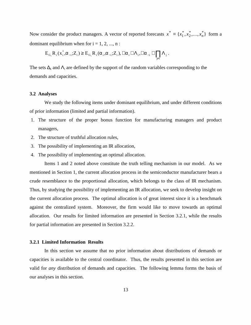
3.1.7 Solution Concepts

We only consider dominant strategy equilibrium as any dominant equilibrium solution is also a

solution for the Bayesian equilibrium. Consider the MMs first. Given an incentive scheme Sk(.)

for MM k, βk k∆∈ is the report of MM k; β-k ∏≠

∆∈kj

j are the reports of all other MMs and bk is

the realization of the random capacity Bk. A vector of reported forecasts x* = {x1*,x2

* ,...,xm* } form

a dominant equilibrium when for k = 1, 2, ..., m:

∏≠

−−− ∆∈β∀∆∈β∀ββ≥βkj

jkkkkkkkFkk*kkF ,,)B;,(SE)B;,x(SE

kk.

13

Now consider the product managers. A vector of reported forecasts x x x xn* * * *{ , ,..., }= 1 2 form a

dominant equilibrium when for i = 1, 2, ..., n :

∏≠

−−− Λ∈α∀Λ∈α∀αα≥αij

jiiiiiiiGii*iiG ,,)Z;,(RE)Z;,x(RE

ii.

The sets ∆k and Λi are defined by the support of the random variables corresponding to the

demands and capacities.

3.2 Analyses

We study the following items under dominant equilibrium, and under different conditions

of prior information (limited and partial information).

1. The structure of the proper bonus function for manufacturing managers and product

managers,

2. The structure of truthful allocation rules,

3. The possibility of implementing an IR allocation,

4. The possibility of implementing an optimal allocation.

Items 1 and 2 noted above constitute the truth telling mechanism in our model. As we

mentioned in Section 1, the current allocation process in the semiconductor manufacturer bears a

crude resemblance to the proportional allocation, which belongs to the class of IR mechanism.

Thus, by studying the possibility of implementing an IR allocation, we seek to develop insight on

the current allocation process. The optimal allocation is of great interest since it is a benchmark

against the centralized system. Moreover, the firm would like to move towards an optimal

allocation. Our results for limited information are presented in Section 3.2.1, while the results

for partial information are presented in Section 3.2.2.

3.2.1 Limited Information Results

In this section we assume that no prior information about distributions of demands or

capacities is available to the central coordinator. Thus, the results presented in this section are

valid for any distribution of demands and capacities. The following lemma forms the basis of

our analyses in this section.

14

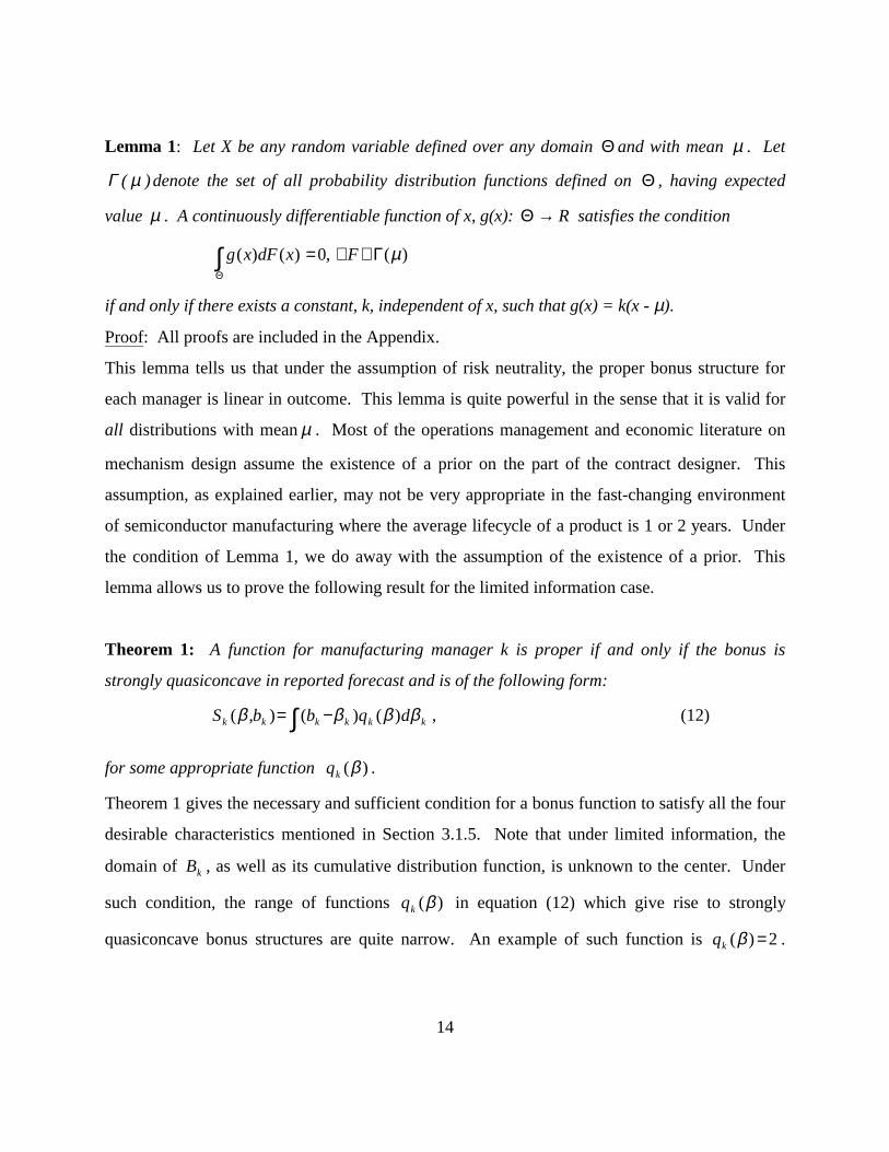
Lemma 1: Let X be any random variable defined over any domain Θ and with mean µ . Let

)( µΓ denote the set of all probability distribution functions defined on Θ , having expected

value µ . A continuously differentiable function of x, g(x): Θ → R satisfies the condition

)(,0)()( µΓ∈∀=∫Θ

FxdFxg

if and only if there exists a constant, k, independent of x, such that g(x) = k(x - µ).

Proof: All proofs are included in the Appendix.

This lemma tells us that under the assumption of risk neutrality, the proper bonus structure for

each manager is linear in outcome. This lemma is quite powerful in the sense that it is valid for

all distributions with mean µ . Most of the operations management and economic literature on

mechanism design assume the existence of a prior on the part of the contract designer. This

assumption, as explained earlier, may not be very appropriate in the fast-changing environment

of semiconductor manufacturing where the average lifecycle of a product is 1 or 2 years. Under

the condition of Lemma 1, we do away with the assumption of the existence of a prior. This

lemma allows us to prove the following result for the limited information case.

Theorem 1: A function for manufacturing manager k is proper if and only if the bonus is

strongly quasiconcave in reported forecast and is of the following form:

∫ −= kkkkkk dqbbS ββββ )()(),( , (12)

for some appropriate function )(βkq .

Theorem 1 gives the necessary and sufficient condition for a bonus function to satisfy all the four

desirable characteristics mentioned in Section 3.1.5. Note that under limited information, the

domain of kB , as well as its cumulative distribution function, is unknown to the center. Under

such condition, the range of functions )(βkq in equation (12) which give rise to strongly

quasiconcave bonus structures are quite narrow. An example of such function is 2)( =βkq .

15

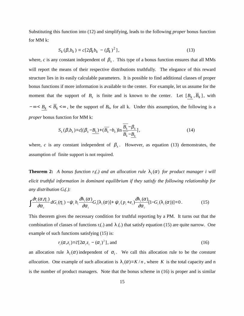
Substituting this function into (12) and simplifying, leads to the following proper bonus function

for MM k:

S b c bk k k k k( , ) [ ( ) ]β β β= −2 2 , (13)

where, c is any constant independent of kβ . This type of a bonus function ensures that all MMs

will report the means of their respective distributions truthfully. The elegance of this reward

structure lies in its easily calculable parameters. It is possible to find additional classes of proper

bonus functions if more information is available to the center. For example, let us assume for the

moment that the support of kB is finite and is known to the center. Let [ , ]B Bk k , with

− ∞< < <∞B Bk k , be the support of Bk, for all k. Under this assumption, the following is a

proper bonus function for MM k:

]ln)()[(),(kk

kkkkkkkk BB

BbBBcbS−−

−+−=βββ , (14)

where, c is any constant independent of kβ . However, as equation (13) demonstrates, the

assumption of finite support is not required.

Theorem 2: A bonus function ri(.) and an allocation rule λi ( )α for product manager i will

elicit truthful information in dominant equilibrium if they satisfy the following relationship for

any distribution Gi(.):

0))]((1[)(

)()]([)(

)(),(

=−++−∫ α∂α

α∂ψα∂α

α∂ψη∂α

ηα∂ii

i

iiiiii

i

iiiii

i

ii GepGhdGr λλ

λλ

. (15)

This theorem gives the necessary condition for truthful reporting by a PM. It turns out that the

combination of classes of functions ri(.) and λ i(.) that satisfy equation (15) are quite narrow. One

example of such functions satisfying (15) is:

])(2[),( 2iiiii zczr ααα −= , and (16)

an allocation rule λi ( )α independent of α i . We call this allocation rule to be the constant

allocation. One example of such allocation is nKi /)( =αλ , where K is the total capacity and n

is the number of product managers. Note that the bonus scheme in (16) is proper and is similar

16

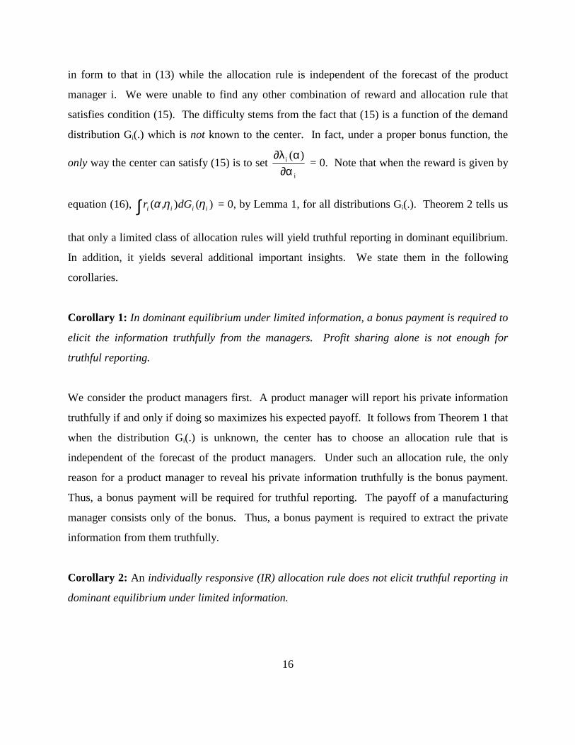
in form to that in (13) while the allocation rule is independent of the forecast of the product

manager i. We were unable to find any other combination of reward and allocation rule that

satisfies condition (15). The difficulty stems from the fact that (15) is a function of the demand

distribution Gi(.) which is not known to the center. In fact, under a proper bonus function, the

only way the center can satisfy (15) is to set i

i )(∂α

α∂λ = 0. Note that when the reward is given by

equation (16), ∫ )(),( iiii dGr ηηα = 0, by Lemma 1, for all distributions Gi(.). Theorem 2 tells us

that only a limited class of allocation rules will yield truthful reporting in dominant equilibrium.

In addition, it yields several additional important insights. We state them in the following

corollaries.

Corollary 1: In dominant equilibrium under limited information, a bonus payment is required to

elicit the information truthfully from the managers. Profit sharing alone is not enough for

truthful reporting.

We consider the product managers first. A product manager will report his private information

truthfully if and only if doing so maximizes his expected payoff. It follows from Theorem 1 that

when the distribution Gi(.) is unknown, the center has to choose an allocation rule that is

independent of the forecast of the product managers. Under such an allocation rule, the only

reason for a product manager to reveal his private information truthfully is the bonus payment.

Thus, a bonus payment will be required for truthful reporting. The payoff of a manufacturing

manager consists only of the bonus. Thus, a bonus payment is required to extract the private

information from them truthfully.

Corollary 2: An individually responsive (IR) allocation rule does not elicit truthful reporting in

dominant equilibrium under limited information.

17

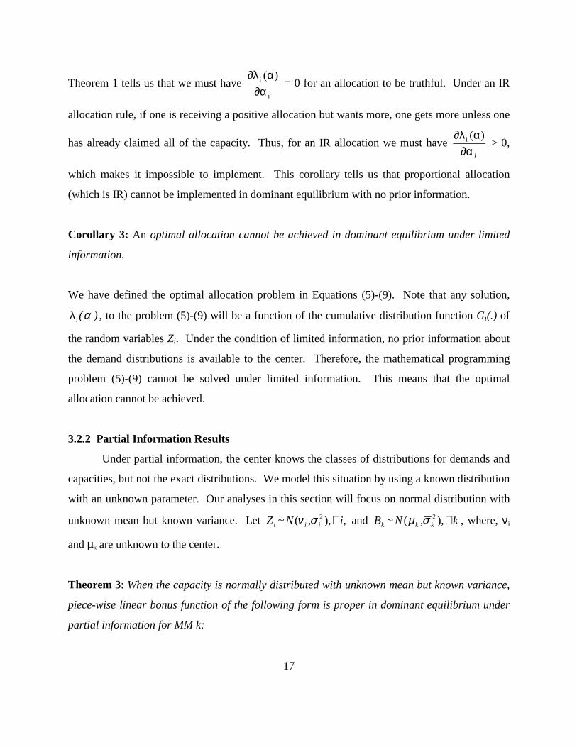
Theorem 1 tells us that we must have i

i )(∂α

α∂λ = 0 for an allocation to be truthful. Under an IR

allocation rule, if one is receiving a positive allocation but wants more, one gets more unless one

has already claimed all of the capacity. Thus, for an IR allocation we must have i

i )(∂α

α∂λ > 0,

which makes it impossible to implement. This corollary tells us that proportional allocation

(which is IR) cannot be implemented in dominant equilibrium with no prior information.

Corollary 3: An optimal allocation cannot be achieved in dominant equilibrium under limited

information.

We have defined the optimal allocation problem in Equations (5)-(9). Note that any solution,

)(i αλ , to the problem (5)-(9) will be a function of the cumulative distribution function Gi(.) of

the random variables Zi. Under the condition of limited information, no prior information about

the demand distributions is available to the center. Therefore, the mathematical programming

problem (5)-(9) cannot be solved under limited information. This means that the optimal

allocation cannot be achieved.

3.2.2 Partial Information Results

Under partial information, the center knows the classes of distributions for demands and

capacities, but not the exact distributions. We model this situation by using a known distribution

with an unknown parameter. Our analyses in this section will focus on normal distribution with

unknown mean but known variance. Let ,),,(~ 2 iNZ iii ∀σν and kNB kkk ∀),,(~ 2σµ , where, νi

and µk are unknown to the center.

Theorem 3: When the capacity is normally distributed with unknown mean but known variance,

piece-wise linear bonus function of the following form is proper in dominant equilibrium under

partial information for MM k:

18

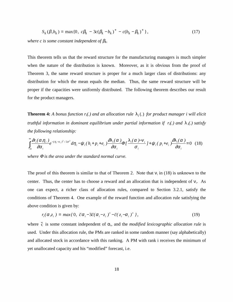
S b c c b c bk k k k k k k( , ) max{ , ( ) ( ) }β β β β= − − − −+ +0 3 , (17)

where c is some constant independent of βk.

This theorem tells us that the reward structure for the manufacturing managers is much simpler

when the nature of the distribution is known. Moreover, as it is obvious from the proof of

Theorem 3, the same reward structure is proper for a much larger class of distributions: any

distribution for which the mean equals the median. Thus, the same reward structure will be

proper if the capacities were uniformly distributed. The following theorem describes our result

for the product managers.

Theorem 4: A bonus function ri(.) and an allocation rule λi (.) for product manager i will elicit

truthful information in dominant equilibrium under partial information if ri(.) and λ i(.) satisfy

the following relationship:

022 2 =++

−++−∫

∞

∞−

−−

i

iiii

i

ii

i

iiiiii

/)(

i

ii )()ep(])([)()eph(de),(rii

∂αα∂ψ

σναΦ

∂αα∂ψη

∂αηα∂ σνη λλλ

(18)

where Φ is the area under the standard normal curve.

The proof of this theorem is similar to that of Theorem 2. Note that νi in (18) is unknown to the

center. Thus, the center has to choose a reward and an allocation that is independent of νi. As

one can expect, a richer class of allocation rules, compared to Section 3.2.1, satisfy the

conditions of Theorem 4. One example of the reward function and allocation rule satisfying the

above condition is given by:

})z(c)z(cc,{max)z,(r iiiiiii++ −−−−= αααα 30 , (19)

where c is some constant independent of αι, and the modified lexicographic allocation rule is

used. Under this allocation rule, the PMs are ranked in some random manner (say alphabetically)

and allocated stock in accordance with this ranking. A PM with rank i receives the minimum of

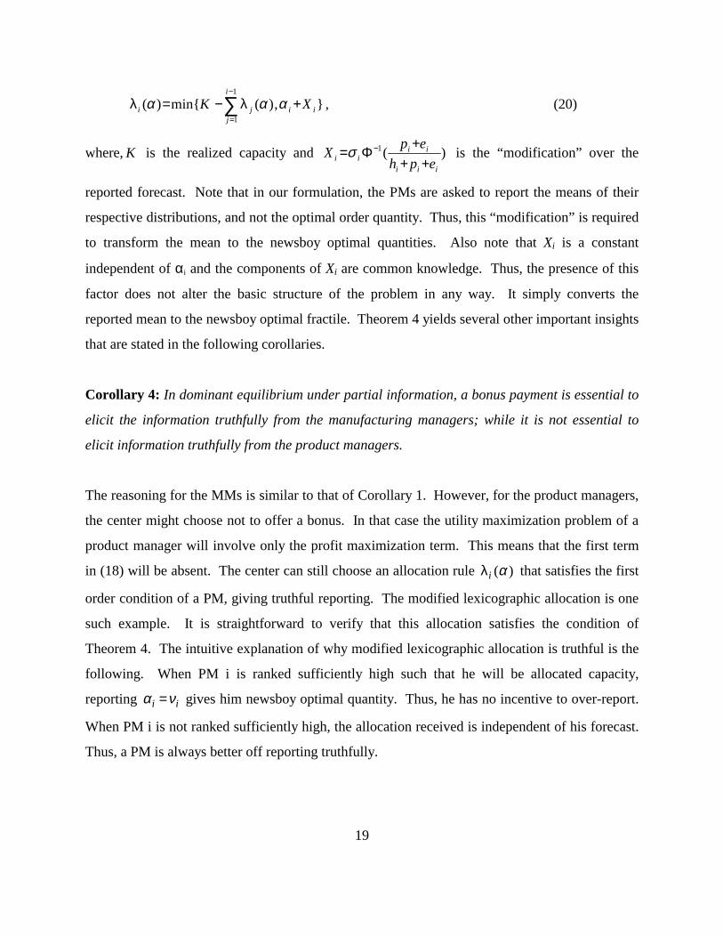
yet unallocated capacity and his “modified” forecast, i.e.

19

},)(min{)(1

1ii

i

jji XK +−= ∑

−

=

ααα λλ , (20)

where, K is the realized capacity and )(1

iii

iiii eph

epX++

+Φ= −σ is the “modification” over the

reported forecast. Note that in our formulation, the PMs are asked to report the means of their

respective distributions, and not the optimal order quantity. Thus, this “modification” is required

to transform the mean to the newsboy optimal quantities. Also note that Xi is a constant

independent of αi and the components of Xi are common knowledge. Thus, the presence of this

factor does not alter the basic structure of the problem in any way. It simply converts the

reported mean to the newsboy optimal fractile. Theorem 4 yields several other important insights

that are stated in the following corollaries.

Corollary 4: In dominant equilibrium under partial information, a bonus payment is essential to

elicit the information truthfully from the manufacturing managers; while it is not essential to

elicit information truthfully from the product managers.

The reasoning for the MMs is similar to that of Corollary 1. However, for the product managers,

the center might choose not to offer a bonus. In that case the utility maximization problem of a

product manager will involve only the profit maximization term. This means that the first term

in (18) will be absent. The center can still choose an allocation rule λi ( )α that satisfies the first

order condition of a PM, giving truthful reporting. The modified lexicographic allocation is one

such example. It is straightforward to verify that this allocation satisfies the condition of

Theorem 4. The intuitive explanation of why modified lexicographic allocation is truthful is the

following. When PM i is ranked sufficiently high such that he will be allocated capacity,

reporting α νi i= gives him newsboy optimal quantity. Thus, he has no incentive to over-report.

When PM i is not ranked sufficiently high, the allocation received is independent of his forecast.

Thus, a PM is always better off reporting truthfully.

20

Corollary 5: Unlike the case of dominant equilibrium with limited information, an individually

responsive (IR) allocation can elicit truthful information in dominant equilibrium under partial

information. However, a bonus is required for its implementation.

The proof is by construction and is included in the Appendix. We have demonstrated the

implementation of a linear allocation rule (which is IR) by appropriate choice of a reward

function. This result is contrary to that of Cachon & Lariviere (1999b). The presence of a bonus

function, in addition to the profit function, in our model allows the implementation of an IR

mechanism by revelation. The intuition behind this is that the center can set the bonus for

truthful forecasting to be sufficiently high so that it compensates a PM for the forgone profit in

terms of product allocation. When capacity is scarce, a PM can gain a greater allocation (hence a

higher profit) by inflating his forecast. However, doing so reduces his bonus payment in an

expected sense. Absence of a bonus scheme makes an IR allocation manipulable in Cachon &

Lariviere (1999b). So far we have not addressed the issue of optimality of allocation. We do so

in the following corollary.

Corollary 6: Given appropriate bonus functions for the MMs and PMs, an optimal allocation

can be implemented by revelation in dominant equilibrium under partial information.

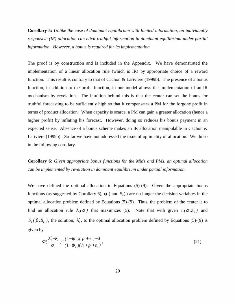
We have defined the optimal allocation in Equations (5)-(9). Given the appropriate bonus

functions (as suggested by Corollary 6), ri(.) and Sk(.) are no longer the decision variables in the

optimal allocation problem defined by Equations (5)-(9). Thus, the problem of the center is to

find an allocation rule )(i αλ that maximizes (5). Note that with given )Z,(r ii α and

)B,(S kk β , the solution, *iλ , to the optimal allocation problem defined by Equations (5)-(9) is

given by

)eph)((

)ep)(()(

iiii

iii

i

i*i

++−−+−

=−

ψλψ

σνΦ

11λ

, (21)

21

where λ is the shadow price of the capacity constraint and Φ is the area under standard normal

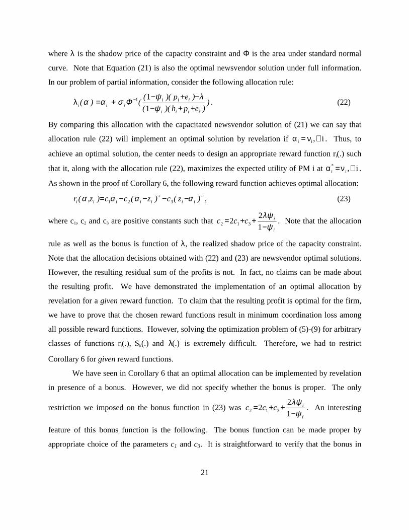
curve. Note that Equation (21) is also the optimal newsvendor solution under full information.

In our problem of partial information, consider the following allocation rule:

))eph)((

)ep)((()(

iiii

iiiiii ++−

−+−+= −

ψλψ

Φσαα111λ . (22)

By comparing this allocation with the capacitated newsvendor solution of (21) we can say that

allocation rule (22) will implement an optimal solution by revelation if α i = νi , ∀ i . Thus, to

achieve an optimal solution, the center needs to design an appropriate reward function ri(.) such

that it, along with the allocation rule (22), maximizes the expected utility of PM i at α i* =νi , ∀ i .

As shown in the proof of Corollary 6, the following reward function achieves optimal allocation:

++ −−−−= )z(c)z(cc)z,(r iiiiiii αααα 321 , (23)

where c1, c2 and c3 are positive constants such that i

icccψ

λψ−

++=12

2 312 . Note that the allocation

rule as well as the bonus is function of λ, the realized shadow price of the capacity constraint.

Note that the allocation decisions obtained with (22) and (23) are newsvendor optimal solutions.

However, the resulting residual sum of the profits is not. In fact, no claims can be made about

the resulting profit. We have demonstrated the implementation of an optimal allocation by

revelation for a given reward function. To claim that the resulting profit is optimal for the firm,

we have to prove that the chosen reward functions result in minimum coordination loss among

all possible reward functions. However, solving the optimization problem of (5)-(9) for arbitrary

classes of functions ri(.), Sk(.) and (.)λ is extremely difficult. Therefore, we had to restrict

Corollary 6 for given reward functions.

We have seen in Corollary 6 that an optimal allocation can be implemented by revelation

in presence of a bonus. However, we did not specify whether the bonus is proper. The only

restriction we imposed on the bonus function in (23) was i

icccψ

λψ−

++=12

2 312 . An interesting

feature of this bonus function is the following. The bonus function can be made proper by

appropriate choice of the parameters c1 and c3. It is straightforward to verify that the bonus in

22

(23) is proper when i

iccψ

λψ−

>>+131 . Thus, a proper bonus function can be used to implement an

optimal allocation by revelation.

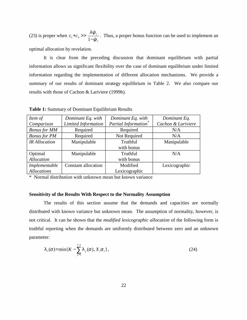
It is clear from the preceding discussion that dominant equilibrium with partial

information allows us significant flexibility over the case of dominant equilibrium under limited

information regarding the implementation of different allocation mechanisms. We provide a

summary of our results of dominant strategy equilibrium in Table 2. We also compare our

results with those of Cachon & Lariviere (1999b).

Table 1: Summary of Dominant Equilibrium Results

Item of Comparison

Dominant Eq. with Limited Information

Dominant Eq. with Partial Information*

Dominant Eq. Cachon & Lariviere

Bonus for MM Required Required N/A Bonus for PM Required Not Required N/A IR Allocation Manipulable Truthful

with bonus Manipulable

Optimal Allocation

Manipulable Truthful with bonus

N/A

Implementable Allocations

Constant allocation Modified Lexicographic

Lexicographic

* Normal distribution with unknown mean but known variance

Sensitivity of the Results With Respect to the Normality Assumption

The results of this section assume that the demands and capacities are normally

distributed with known variance but unknown mean. The assumption of normality, however, is

not critical. It can be shown that the modified lexicographic allocation of the following form is

truthful reporting when the demands are uniformly distributed between zero and an unknown

parameter:

},)(min{)(1

1ii

i

jji XK ααα ∑

−

=

−= λλ , (24)

23

where, the modification is given by X i =2(pi +ei )hi + pi +ei

. The parameters in the expression of Xi are,

again, common knowledge. Similarly, the bonus function given by (16) is also proper under

uniform distribution. The other results of normal distribution (with unknown mean) also carry

over to the case of uniform distribution.

4.0 IMPLICATIONS FOR PRACTITIONERS

Our model provides the following insights for the practitioners. The current allocation

practice in the firm bears a crude resemblance to the proportional allocation scheme. This

allocation falls under the broad category of the IR allocation rules described earlier. Our analyses

suggest that this allocation is truthful only under partial information and in presence of a bonus.

Thus, in order to get truthful reporting under this allocation, in addition to a bonus, the central

coordinator needs to have a rough idea about the distributions. Under the existing incentive

system of the firm, there is no explicit bonus associated with forecasting. This explains the

gaming behavior of the concerned managers.

Under the current allocation procedure, the central coordinator does not take into account

the differential product margins. However, the firm is interested in putting together an allocation

mechanism that maximizes the total profit of the firm. This translates into moving towards an

optimal allocation described herein. Our analyses, again, suggest that this allocation is truthful

only under partial information and in presence of a bonus. Thus, in order to get truthful reporting

under this allocation, in addition to a bonus, the central coordinator again needs to have a rough

idea about the distributions.

Under the current compensation structure of the firm, the pay of a manager is the sum of

two components: the fixed pay element and the variable pay element. The fixed pay element

consists of two elements, the base salary and the annual pay raise. The variable pay element

consists of the firm award and unit award. The firm award is dependent on the overall

performance of the firm (earnings per share). The unit award received by a business unit (the

semiconductor manufacturer described in this paper is the microelectronics business unit of the

24

firm) is a percentage of the net operating income generated by that business unit on a global

basis. We note that currently there is no explicit bonus for forecast accuracy. Our analyses

suggest that an explicit forecast-related bonus is required for the managers. The central

coordinator indicated that it is possible to disburse the unit award as per bonus schemes

developed in this research.

We note that our work is motivated by the experiences of a major US-Based

semiconductor manufacturer. However, similar problems are not uncommon to other firms.

Pich and Harrison (1990) noted similar problems in a case study (American Semiconductor, Inc.

(A) – Service Systems Architecture, Stanford University Case # S-DS-88A). They noted that the

said firm was facing the problem of under-forecasting by their manufacturing managers and over-

forecasting by their product managers. However, they did not study the problem formally. Our

modeling framework is also general enough to be adapted to other resource allocation problems

under asymmetric information.

5.0 SUMMARY AND DIRECTIONS FOR FUTURE RESEARCH

In this paper, we have proposed a game theoretic model of incentive problems in

forecasting and capacity allocation. Our problem is one of hidden information. The

distinguishing feature in our model is the presence of the multiple manufacturing managers. We

have developed a theoretical framework to analyze the incentive structure required for truthful

reporting under different conditions of information availability. We have also characterized

which allocation rules are truthful. We have compared our results with those from literature.

Our analyses assume a new feature on information availability condition: the limited information

case. To our knowledge, no other work in operations management literature has studied a similar

case. The coordination literature in operations management always assumes the existence of a

prior. However, the assumption of limited information is becoming increasingly relevant in a

fast-changing world. We have shown that only constant allocation is truthful under such

conditions and that a bonus is required for all managers for truthful reporting. Under the

condition of partial information, the modified lexicographic allocation is shown to be truthful. In

addition, the optimal allocation and the IR allocation are also truthful with bonus.

25

We have assumed risk neutrality. We note that virtually all coordination models reported

in operations management literature (Porteus & Whang, 1991; Cachon & Lariviere, 1999a, b;

Corbett, 1996) assume risk neutrality. This assumption allowed us to compare and contrast our

work with the literature. The main contribution of our model is in considering multiple

manufacturing managers and developing an integrated framework of forecasting and product

allocation. In spite of our specific emphasis on semiconductor manufacturing, the analytical

results presented in this paper are general enough to be used in other coordination problems. We

identify the following directions for our future research.

• Reporting of Multiple Statistics: This paper assumes that the PMs and the MMs report only a

single statistics (the mean) about their respective distribution. A natural extension to this

idea is to ask them to report multiple statistics (mean and standard deviation, for example)

and to design a mechanism that induces truthful reporting of multiple statistics.

• Exploring Market Mechanisms: A natural extension to our work is to look for a market

mechanism based on auctions/bidding to allocate the available capacities. The specific issues

to look at will be the following. What is the structure of the auction (for example a PM bids

for capacities or a MM submits asks for available capacities)? What are the allocation

decisions and coordination costs under an auction-based method? How does an auction-

based method compare with optimization-based method (our current approach)?

• Extension to Random Yield Problems: An extension to the optimal allocation problem

described here is the decentralized random yield problem. Under such a situation, the MMs

report their respective yields (a 0-1 random variable). Allocation is based on these reports.

The optimal allocation, thus, becomes a stochastic programming problem.

26

REFERENCES Atkinson, A.A., “Incentives, Uncertainty and Risk in the Newsboy Problem,” Decision Sciences,

Vol. 10, pp. 341-357, 1979. Axsater, S., “Continuous Review policies for Multi-Level Inventory Systems with Stochastic

Demand,” in Handbooks in OR & MS, Vol.4, S.C. Graves et al. (ed.), Elsevier, 1993.

Bazaraa, M.S., C.M. Shetty, Nonlinear Programming: Theory and Algorithms, John Wiley, NY,

1979. Cachon, G.P., M.A. Lariviere, “Capacity Allocation Using Past Sales: When to Turn-and-Earn,”

Management Science, 45 (5) 685-703, 1999a. Cachon, G.P., M.A. Lariviere, “Capacity Choice and Allocation: Strategic Behavior and Supply

Chain Performance,” Management Science, 45 (8) 1091-1108, 1999b. Clark, A.J., H. Scarf, “Optimal Policies for a Multi-Echelon Inventory Problem,” Management

Science, Vol. 6, No. 4, pp. 475-490, 1960. Corbett, C., “Consignment Stock and Demand Variability in an Imperfect Supply Chain

Partnership,” Unpublished dissertation, INSEAD, 1996. Eppen, G.D., “Effects of Centralization on Expected Costs in a Multi-Location Newsboy

Problem,” Management Science, 25, 5, pp. 498-501, 1979 Fudenberg, D., J. Tirole, Game Theory, MIT Press, Cambridge, MA, 1991. Gilbert, S.M., Z.K. Weng, “Incentive Effects Favor Non-Consolidating Queues in a Service

System: The Principal-Agent Perspective, Working Paper, Case Western Reserve University, 1997.

Gonik, J., “Tie Salesmen’s Bonuses to Their Forecasts,” Harvard Business Review, 56, pp. 116-

123, May-June, 1978 Grout, J.R., D.P. Christy, “An Inventory Model of Incentives for On-Time Delivery in Just-in-

Time Purchasing Contracts,” Naval Research Logistics, Vol. 40, pp. 863-877, 1993. Grout, J.R., “A Model of Incentive Contracts for Just-In-Time Delivery,” Working Paper,

Southern Methodist University, 1996. Groves, T., M. Loeb, “Incentives in a Divisionalized Firm,” Management Science, Vol 25, No. 3,

pp. 221-230, 1979.

27

Harris, M., C.H. Kriebel, A. Raviv, “Asymmetric Information, Incentives and Intrafirm Resource

Allocation,” Management Science Vol. 28, No. 6, pp. 604-620, 1982. Hauser, J.R., D.I. Simester, B. Wernerfelt, “Internal Customers and Suppliers,” Working Paper,

MIT, 1994. Kandel, E., “The Right to Return,” Journal of Law and Economics, April, 1996. Lee, H., S. Whang, “Decentralized Multi-Echelon Inventory Control Systems: Incentives and

Information,” Working Paper, Stanford University, 1994. Lee, H., P. Padmanabhan, S. Whang, “Information Distortion in a Supply Chain: The Bullwhip

Effect,” Management Science, Vol. 43, No. 4, pp.546-558, 1997. Milgrom, P.R., R.J. Weber, “Distributional Strategies for Games with Incomplete Information,”

Mathematics of Operations Research, Vol. 10, pp. 619-631, 1986. Pich, M.T., J.M. Harrison, American Semiconductor, Inc. (A) – Service Systems Architecture,

Stanford University Case # S-DS-88A, 1990. Porteus, E.L., S. Whang, “On Manufacturing/Marketing Incentives,” Management Science, Vol.

37, No. 9, pp. 1166-1181, 1991. Tsay, A.A., S. Nahmias, N. Agrawal, “Modeling Supply Chain Contracts: A Review,” In S.

Tayur et al., (Eds.), Quantitative Models for Supply Chain Management, pp. 299-336, Kluwer Academic Publishers, 1999.

Van Ackere, A., “The Principal/Agent Paradigm: Its Relevance to Various Functional Fields,”

European Journal of Operational Research, Vol. 70, pp. 83-103, 1993. Whang, S., “Coordination in Operations: A Taxonomy,” Journal of Operations Management, 12,

pp. 413-422, 1995.

28

APPENDIX : PROOFS OF THEOREMS

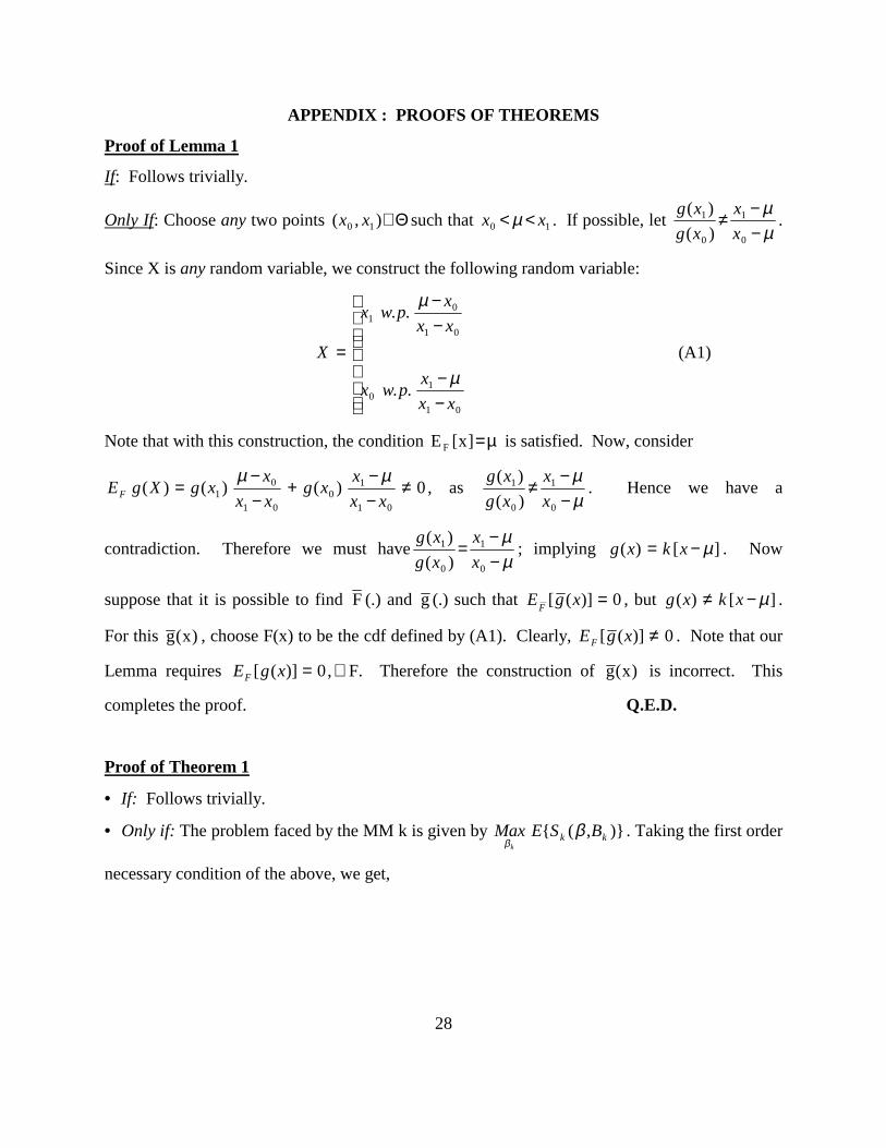
Proof of Lemma 1

If: Follows trivially.

Only If: Choose any two points Θ∈),( 10 xx such that 10 xx <<µ . If possible, let µµ

−−

≠0

1

0

1

)()(

xx

xgxg

.

Since X is any random variable, we construct the following random variable:

−−

−−

=

01

10

01

01

..

..

xxxpwx

xxxpwx

Xµ

µ

(A1)

Note that with this construction, the condition µ=]x[E F is satisfied. Now, consider

0)()()(01

10

01

01 ≠

−−

+−−

=xx

xxgxxx

xgXgEFµµ

, as µµ

−−

≠0

1

0

1

)()(

xx

xgxg

. Hence we have a

contradiction. Therefore we must haveµµ

−−

=0

1

0

1

)()(

xx

xgxg

; implying ][)( µ−= xkxg . Now

suppose that it is possible to find F (.) and g (.) such that 0)]([ =xgEF , but ][)( µ−≠ xkxg .

For this )x(g , choose F(x) to be the cdf defined by (A1). Clearly, 0)]([ ≠xgEF . Note that our

Lemma requires ∀= ,0)]([ xgEF F. Therefore the construction of )x(g is incorrect. This

completes the proof. Q.E.D.

Proof of Theorem 1

• If: Follows trivially.

• Only if: The problem faced by the MM k is given by )},({ kk BSEMaxk

ββ

. Taking the first order

necessary condition of the above, we get,

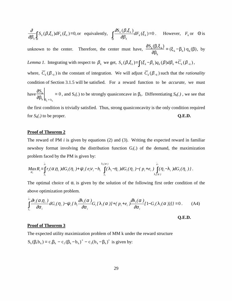
29

,0)(),( =∫Θ

kkkkk

dFS ξξβ∂β∂ or equivalently, 0)(

),(=∫

Θkk

k

kk dFS ξ

∂βξβ∂

. However, kF or Θ is

unknown to the center. Therefore, the center must have, ∂Sk (β,ξ k )

∂βk

= (ξ k −βk ) qk (β), by

Lemma 1. Integrating with respect to kβ we get, )()()(),( kkkkkkkk CdqS −+−=∫ ββββξξβ ,

where, )( kkC −β is the constant of integration. We will adjust )( kkC −β such that the rationality

condition of Section 3.1.5 will be satisfied. For a reward function to be accurate, we must

have∂Sk

∂βk βk = bk

= 0 , and Sk(.) to be strongly quasiconcave in βk. Differentiating Sk(.) , we see that

the first condition is trivially satisfied. Thus, strong quasiconcavity is the only condition required

for Sk(.) to be proper. Q.E.D.

Proof of Theorem 2

The reward of PM i is given by equations (2) and (3). Writing the expected reward in familiar

newsboy format involving the distribution function Gi(.) of the demand, the maximization

problem faced by the PM is given by:

})(dG)()ep()(dG)(he{)(dG),(rRMaxi

i

i

i

i

ii

z

)(iiiiii

)(

ziiiiiiii

z

ziiiii ∫∫∫ −+−−−+=

α

α

αηηηηνψηηα

λ

λ

λλ .

The optimal choice of αi is given by the solution of the following first order condition of the

above optimization problem.

01 =−++−∫ ))]}((G[)(

)ep()]([G)(

h{)(dG),(r

iii

iiiii

i

iii

z

zii

i

iii

i

α∂α

α∂α∂α

α∂ψη∂α

ηα∂λ

λλ

λ. (A4)

Q.E.D.

Proof of Theorem 3

The expected utility maximization problem of MM k under the reward structure

Sk (β,bk ) = c1βk − c2 (βk −bk )+ − c3(bk −βk )+ is given by:

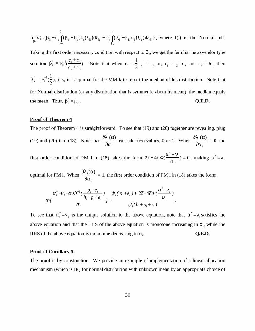
30

maxβ k

{ c1βk −c2 (βk −ξk )fk (ξ k )dξk−∞

β k

∫ − c3 ( ξk −βk )fk (ξ k )dξ kβ k

∞

∫ }, where f(.) is the Normal pdf.

Taking the first order necessary condition with respect to βk, we get the familiar newsvendor type

solution βk* = Fk

−1(c1 +c3

c2 +c3). Note that when c1 =

13

c2 = c3 , or, c1 = c3 =c , and c2 = 3c , then

βk* = Fk

−1(12

), i.e., it is optimal for the MM k to report the median of his distribution. Note that

for Normal distribution (or any distribution that is symmetric about its mean), the median equals

the mean. Thus, βk* =µk . Q.E.D.

Proof of Theorem 4

The proof of Theorem 4 is straightforward. To see that (19) and (20) together are revealing, plug

(19) and (20) into (18). Note that i

i )(∂α

α∂λ can take two values, 0 or 1. When

i

i )(∂α

α∂λ = 0, the

first order condition of PM i in (18) takes the form 2c −4c Φ(α i* − νi

σ i) = 0 , making α i

* =ν i

optimal for PM i. When i

i )(∂α

α∂λ = 1, the first order condition of PM i in (18) takes the form:

)eph(

)(cc)ep(]

)eph

ep([

iiii

i

i*i

iii

i

iii

iiii

*i

++

−−++

=++

++− −

ψσ

ναΦψ

σ

ΦσναΦ

421

.

To see that α i* =ν i is the unique solution to the above equation, note that α i

* =ν i satisfies the

above equation and that the LHS of the above equation is monotone increasing in αi, while the

RHS of the above equation is monotone decreasing in αi. Q.E.D.

Proof of Corollary 5:

The proof is by construction. We provide an example of implementation of a linear allocation

mechanism (which is IR) for normal distribution with unknown mean by an appropriate choice of

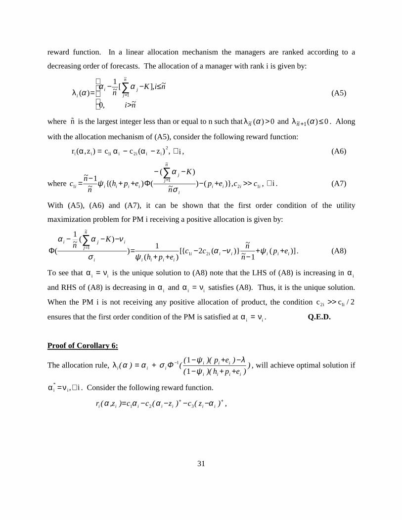
31

reward function. In a linear allocation mechanism the managers are ranked according to a

decreasing order of forecasts. The allocation of a manager with rank i is given by:

>

≤−−= ∑

=

ni

niKn

n

jji

i~,0

~,][~1

)(

~

1

αααλ (A5)

where ˜ n is the largest integer less than or equal to n such that λ~ ( )n α >0 and λ~ ( )n + ≤1 0α . Along

with the allocation mechanism of (A5), consider the following reward function:

ri (α ,zi ) = c1i α i − c2i(α i − zi)2, ∀ i , (A6)

where iiiii

n

jj

iiiii ccepn

Keph

nnc 12

~

11 )},()~

)(()({~

1~>>+−

−−Φ++−=

∑=

σ

αψ , ∀ i . (A7)

With (A5), (A6) and (A7), it can be shown that the first order condition of the utility

maximization problem for PM i receiving a positive allocation is given by:

)](1~

~)}(2{[

)(1)

)(~1

( 21

~

1iiiiiii

iiiii

i

n

jji

epn

ncceph

Kn

++−

−−++

=−−−

Φ∑

= ψναψσ

ναα. (A8)

To see that α i = νi is the unique solution to (A8) note that the LHS of (A8) is increasing in α i

and RHS of (A8) is decreasing in α i and α i = νi satisfies (A8). Thus, it is the unique solution.

When the PM i is not receiving any positive allocation of product, the condition c2i >> c1i / 2

ensures that the first order condition of the PM is satisfied at α i = νi . Q.E.D.

Proof of Corollary 6:

The allocation rule, ))eph)((

)ep)((()(

iiii

iiiiii ++−

−+−+= −

ψλψ

Φσαα111λ , will achieve optimal solution if

α i* =νi , ∀ i . Consider the following reward function.

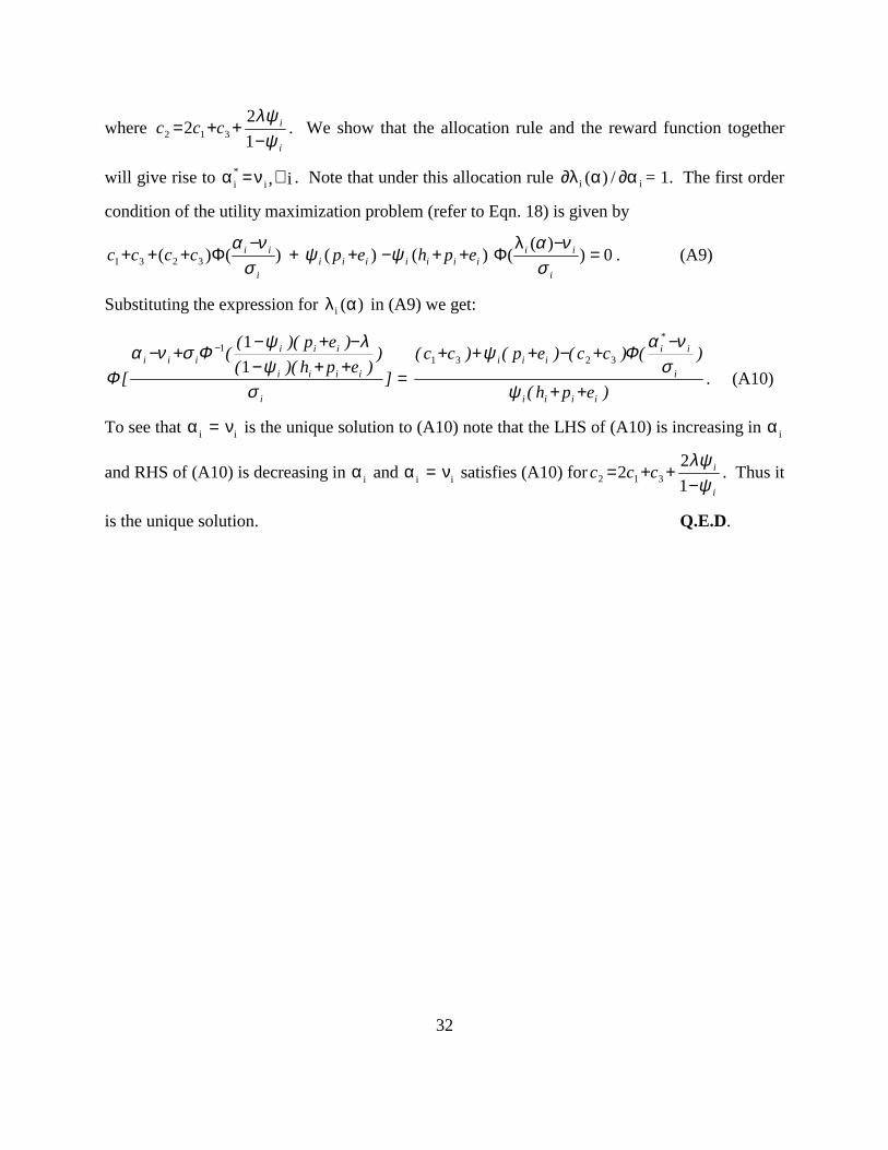
++ −−−−= )z(c)z(cc)z,(r iiiiiii αααα 321 ,

32

where i

icccψ

λψ−

++=12

2 312 . We show that the allocation rule and the reward function together

will give rise to α i* =νi , ∀ i . Note that under this allocation rule ii /)( ∂αα∂λ = 1. The first order

condition of the utility maximization problem (refer to Eqn. 18) is given by

0))(

()()()()( 3231 =−

Φ++−++−

Φ+++i

iiiiiiiii

i

ii ephepccccσ

ναψψ

σνα λ

. (A9)

Substituting the expression for )(i αλ in (A9) we get:

)eph(

)()cc()ep()cc(]

))eph)((

)ep)((([

iiii

i

i*i

iii

i

iiii

iiiiii

++

−+−+++

=++−−+−

+− −

ψσ

ναΦψ

σψ

λψΦσναΦ

32311

11

. (A10)

To see that α i = νi is the unique solution to (A10) note that the LHS of (A10) is increasing in α i

and RHS of (A10) is decreasing in α i and α i = νi satisfies (A10) fori

icccψ

λψ−

++=12

2 312 . Thus it

is the unique solution. Q.E.D.