SEISMIC SOIL-STRUCTURE INTERACTION RESPONSE OF INELASTIC

SEISMIC SOIL-STRUCTURE INTERACTION RESPONSE OF INELASTIC STRUCTURES

Sittipong Jarernprasert, Enrique Bazan-Zurita

Paul C. Rizzo Associates, Inc., Pittsburgh, PA 15235 Jacobo Bielak

Carnegie Mellon University, Pittsburgh, PA 15213 Dedicated to José M. Roësset; scholar, teacher and friend

SUMMARY

We analyze the effects of soil-structure interaction (SSI) on the response of yielding single-story structures

embedded in an elastic halfspace to a set of accelerograms recorded in California and to a set of records

from Mexico City. We find that, for nonlinear hysteretic structures, SSI may lead to larger ductility

demands and larger total displacements than if the soil were rigid. This behavior differs from that

envisioned in current seismic provisions, which allow designers to ignore SSI altogether or to reduce the

base shear force with respect to that of the fixed-base structure. To overcome this deficiency, we examine

an approach to incorporate SSI in determining the seismic design coefficient, yC~ , of systems with non-

structural degrading elastoplastic behavior and target ductility μt. In this approach, yC~ is obtained as the

unreduced seismic coefficient, C, of an equivalent fixed-base structure with natural period T~ , the natural

period of the elastic SSI system, and with inelastic reduction factor equal to the λ-root of the fixed-base

reduction factor, where λ = TT~ , and T is the elastic natural period of the structure ignoring SSI. The

peak relative displacement of the structure can be evaluated as the yield displacement yu~ times the target

ductility μt. The peak total displacement, including SSI, is closely approximated by yu~ (μt + λ2 – 1).

Keywords: seismic response, seismic design, seismic analysis, inelastic structure, inelastic

response, soil-structure interaction

1. INTRODUCTION

Current seismic design provisions allow engineers to completely ignore the effects of soil-

structure interaction in the seismic analysis of buildings, or to consider them by reducing the

design base shear of the fixed-base structure (e.g., ASCE [1]; NTDF [2], NEHRP [3]). A

discussion of the SSI prescriptions of NEHRP has been presented by Stewart et al [4]. These

provisions are based on analyses of simple linear, viscously damped, structures subjected to

transient or steady-state excitation (e.g., Bielak [5]; Jennings and Bielak [6]; Veletsos and Meek

[7]; Luco [8]; Roesset, [9]), and reflect the observation that interaction produces an elongation of

the fixed-base natural period and dissipation of part of the vibrational energy of the building by

Soil Dynamic and Earthquake Engineering Journal

© Paul C. Rizzo Associates, Inc.

2

wave radiation into the foundation medium (in addition to energy losses from internal friction in

the soil). The increase in period results in an increase of the seismic coefficient on an ascending

branch of the response spectrum, no change on a flat portion, and a decrease in a descending

branch. In addition, the energy dissipated in the foundation will usually increase the effective

damping, and, therefore, tend to decrease the spectral ordinate. Past studies show that for linear

systems, the effects of soil-structure interaction are, on balance, beneficial, and are the basis for

allowing a reduction in the base shear in seismic design provisions.

While linear analysis provides valuable insight into the response to earthquake excitation,

most real structures behave nonlinearly, particularly for the seismic intensities implied in design

spectra. In contrast to the extensive work devoted to date to linear SSI, less attention has been

given to nonlinear structural and soil behavior in SSI studies. Among these studies, earthquake

response of building-foundation systems with elastoplastic soil behavior has been studied by

Isenberg [10] and Minami [11]. Kobori et al [12] and Inoue et al [13] considered, in addition,

elastoplastic structures, but restricted their attention to lateral displacements of the base mass.

Veletsos and Verbic [14] studied the response of single-story elastoplastic structures on an elastic

halfspace to a simple pulse and found that the differences between the spectra obtained

considering SSI and the associated nonlinear fixed-base systems are significantly smaller than

those for elastic structures, the differences decreasing with increasing ductility ratio. In a study of

the steady-state response of a simple bilinear hysteretic structure supported on an elastic

halfspace, Bielak [15] found that, contrary to linear systems, SSI can cause the resonant

amplitude of the response of the hysteretic structure to increase over that for a rigid foundation.

The same general behavior has been observed more recently by Mylonakis and Gazetas [18], and

by Avilés and Pérez-Rocha [19]. The latter have proposed a simple fixed-base replacement

oscillator approach using an effective ductility, together with the known effective period and

damping of the system for the elastic condition, to account for the interaction effects of the

coupled system.

In this paper, we examine the response of single-story inelastic structures, with a foundation

embedded in an elastic halfspace, with a view towards (a) assessing the importance of SSI effects

in yielding structures; (b) evaluating current seismic design provisions for taking these effects

into consideration; and (c) developing an approach for the seismic design of SSI systems and to

calculate the corresponding nonlinear structural displacement.

As seismic input we selected two ensembles of earthquake records, corresponding to two

different geological settings: The first consists of 87 accelerograms recorded in California at sites

ranging from hard to medium hard, with a few soft sites. The second set comprises 66 records



3

from the soft lakebed of Mexico City. The records are normalized to have the same Arias

intensity and also with respect to the mean peak ground acceleration, PGA , and have the average

5 percent damped elastic spectra presented in Fig.1. These numbers of records and their

normalization result in smooth average spectra. Inelastic spectra are even smoother (Jarernprasert

et al [20]), enabling us to examine code specifications that prescribe design spectra and inelastic

reduction factors that exhibit smooth variations with period. The source, geological settings and

site conditions are reflected in the periods where the peak spectral ordinates occur at 0.3 s for the

California records and at 2.0 s for the Mexican accelerograms.

Before examining the behavior of inelastic structures on flexible foundations, in the following

two sections we summarize two related cases that serve as the points of departure for our study:

1) an inelastic structure on a fixed base, and 2) an elastic structure with a flexible base (elastic

SSI system).

2. PRIOR STUDY OF INELASTIC STRUCTURES ON A FIXED-BASE

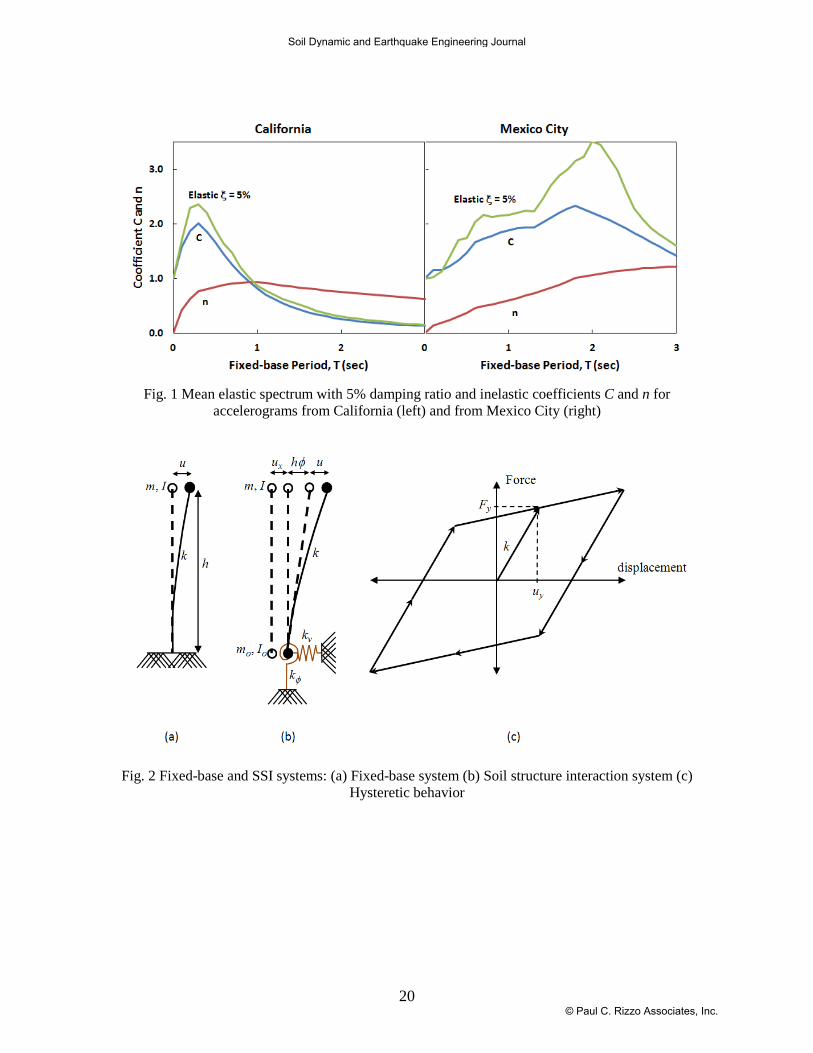
The single-story structure supported on a fixed base shown in Fig. 2, was examined

previously by the authors. The structure has an elastic period T and non-degrading bilinear

hysteretic behavior defined by a yield displacement, uy, and slope of the second branch of the

skeleton force-displacement relationship assumed to be 2 percent of the initial slope, also shown

in Fig. 2. The seismic coefficient is defined as Cy = Vy /W, in which Vy = k uy, with k = m (2π/T).

k is the stiffness of the structure, m its mass, Vy is the base shear, and W = mg, the weight of the

structure.

Jarernprasert et al [20, 21] found that the value of Cy that results in an average ductility

demand, µ , corresponding to the two set of earthquakes base motion can be closely estimated as

)(/)(),( TnTCTyC µµ = (1)

The two quantities C and n depend only on the elastic natural period, T. C(T) differs

somewhat from the elastic spectrum and can be interpreted as a pseudo-elastic design spectrum

corresponding to µ = 1. The denominator )(TnR µ= constitutes a reduction factor that accounts

for inelastic energy dissipation. Close forms for C and n for the two sets of earthquakes records

considered herein are given in [20].

3. SEISMIC RESPONSE OF ELASTIC SSI SYSTEMS



4

Procedures for taking SSI into consideration in the seismic design of buildings are based

primarily on studies of the response of single-story elastic models as the one illustrated in Fig. 2,

where the impedance of the foundation and surrounding soil is represented by translational, kv,

and rotational, kφ, elastic springs and their associated viscous dampers. Following Jennings and

Bielak [5], the SSI fundamental period, T~ , can be closely estimated as:

φk

khkk

TT

v

2

1~

++= (2)

Supertildes will be used throughout to denote quantities associated with the SSI system. h is

the effective height of the structure. Assuming that the fixed-base structure has 5 percent critical

damping, the effective damping ratio, β~ , of the SSI system is (Jennings and Bielak [5]):

3

~05.0~

+=

TT

oββ (3)

βo is the contribution to the effective damping ratio due to geometric scattering and intrinsic

damping in the soil, which depends on TT~ and h/r. With reference to the bearing area of the

foundation, r is the radius of the circle with the same area, for squatty buildings, or with the same

moment of inertia about a centroidal axis perpendicular to the direction of the motion, for slender

buildings. The second term is the modified structural damping due to SSI.

The seismic design coefficient for the SSI system is obtained by entering into the fixed-base

spectrum with T~ . Due to the change in damping, this coefficient must be modified, because β~ in

general differs from 0.05. For instance, one may use the recommendation of Arias and Husid [22]

by scaling the original spectrum by the factor (0.05/ β~ )0.4.

Now, let the ratio TT~ be denoted by λ. Then:

T~ = λT (4)

305.0~ −+= λββo

(5)

In this study, we take λ to vary between 1.1 and 1.5, and take the slenderness ratio H/B equal

to 2, where H is the total height of the structure, and B is the base dimension of the foundation,

considered to be square. We have taken r = B/1.75, and h = 0.7H. To calculate kv, kφ, and the SSI

damping ratios we use formulas by Gazetas [23] and NEHRP [3]. Details are provided in

Appendix B. In addition, only ground motion in one horizontal direction is investigated and we

consider only inertial interaction. As indicated by Avilés and Pérez-Rocha [24], kinematic



5

interaction is not as significant as inertial interaction for typical building-foundation systems and

geological settings.

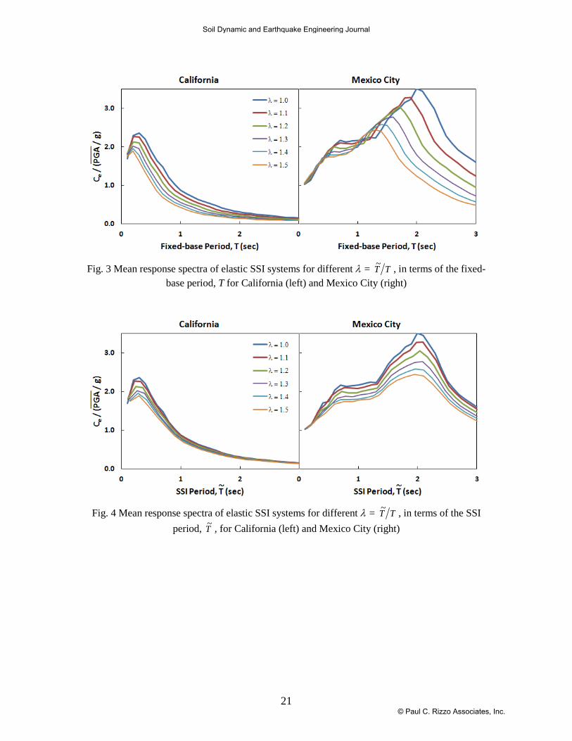
Having completely specified the SSI system for a prescribed value of λ = TT~ , we could

calculate its response for different periods T and different value of λ, for the two sets of

excitations. We interpret λ as a metric of the amount of interaction in the system. The mean

elastic seismic coefficient, WeVeC /= , is shown in Fig. 3. eV is the mean base shear force of

the elastic structure. The left panel of Fig. 3 corresponds to the California accelerograms and

shows that, practically for all periods, an increase in λ reduces the base shear with respect to the

fixed-base case (λ = 1). In addition, the slight shift of the peak spectral value towards the left

reflects the increase in the effective natural period of the SSI system. The right panel displays

the average spectra obtained with the Mexican records, which show that increasing λ reduces the

shear force for fixed-base periods greater than the dominant period of 2 sec and for periods lower

than 1 sec. For intermediate periods, the response shows a small increase.

Figure 4 displays the same spectra as in Fig. 3 but with the SSI period, T~ , in the abscissa.

This display shows clearly that the peak shear forces for different values of λ are all aligned and

occur at a period T~ equal to the dominant period of the seismic input. For all periods, smaller

spectral values are obtained as the flexibility of the soil increases, thus reflecting the effect of the

SSI damping.

4. SEISMIC RESPONSE OF SSI SYSTEMS WITH INELASTIC STRUCTURES

With the previous preamble, we now proceed to study again the earthquake response of the

SSI systems studied in the previous section, but considering now that the structure in Fig. 2

exhibits the hysteretic behavior depicted in the same figure. The need for this study is attested by

the example presented in Appendix C which shows that the base flexibility can increase the

ductility demand on the superstructure.

The seismic coefficient is now defined as yC~ = yV~ /W, where yV~ = k yu~ is the structure yield

force. Values of yC~ that lead to a prescribed average ductility are determined as follows:

• Select λ and a target ductility demand µt;

• For each fixed-based period, T, and prescribed λ, define the properties of the elastic SSI

system as described in Appendix B;



6

• For a given set of records, find the minimum yC~ for which the response of the

superstructure remains elastic for all records;

• Progressively reduce yC~ and set the yield displacement as:

yu~ = yV~ /k = W yC~ /k = yC~ T 2 g / (2π)2 (6)

• For each yC~ and each earthquake record, solve numerically the nonlinear differential

equations of motion of the system. Obtain the maximum relative displacement of the

structure, umax, and the resulting ductility demand, µ = umax/ yu~ ; μ can be less than unity;

• Calculate the mean µ from the results for all the records in the set, assuming that µ has a

lognormal distribution, as explained by Jarernprasert [21];

• By interpolating between closely spaced values of yC~ , determine yC~ such that µ equals

µt. Whereas for an individual earthquake record the relationship between µ and yC~ is

not necessarily unique (e.g., see Chopra, [25], p.256), we found a one-to-one

correspondence between yC~ and µ .

In all SSI systems we consider H/B = 2.

Figure 5 shows yC~ when µt equals 2, for λ between 1 (fixed-base case) and 1.5, as a function

of the SSI-period T~ . For a given period, the seismic coefficient yC~ increases as the SSI effects,

as measured by λ = TT~ , increase. This behavior, opposite to that exhibited by elastic SSI

systems, indicates that as the soil becomes softer, the structure deforms less and dissipates less

energy than when the soil is stiffer. The additional energy dissipated in the soil is not sufficient to

compensate for the reduced hysteretic energy in the superstructure. Thus, there is a need for a

higher yC~ to maintain µt = 2 as λ increases. The spread of spectral values is most pronounced

where the SSI period equals the dominant period of the input set of earthquake records

(approximately 0.3 sec for the California set and 2.0 sec for the Mexico City set). Also, the

peaks of the spectra shift slightly to the right for increasing λ, as a consequence of the lengthening

of the effective natural period of the superstructure caused by its inelastic behavior.

Figure 6 shows again yC~ in terms of T~ , but now for a target ductility demand of 4. Again,

yC~ increases with λ, but this time the peaks for SSI periods are significantly flatter, revealing that

just as for fixed-base systems, increasing inelastic behavior in the structure tends to eliminate the

peaks that characterize elastic spectra.



7

5. EVALUATION OF CURRENT SEISMIC SSI PROVISIONS

In contrast to the result in the preceding section, building codes generally allow (1) a

reduction of the overall seismic coefficient on account of SSI, or (2) SSI effects to be ignored. In

this section we examine these two courses of action on the ductility demand. First, we study the

option of reducing the seismic coefficient for a set of fixed-based periods, T, by means of the

following steps for each T:

• Select the ratio of SSI period to fixed-base period, λ = TT~ , of the system, and a target

ductility µt;

• Calculate T~ = λT and the increased damping ratio of the equivalent linear oscillator, β~ ,

e.g., with (3);

• Reduce the elastic fixed-base seismic coefficient at the period T. We use the

prescriptions of ASCE 7-10 [1] which account for reductions due to elongated period T~

and for the increased damping ratio β~ .

• To incorporate the nonlinear structural effect, calculate the fixed-base inelastic reduction

factor, )(TntR µ= which leads to a mean ductility demand µt in the fixed-based system;

• Apply R to reduce the elastic fixed-base seismic coefficient;

• Analyze the SSI system, and calculate resulting the mean ductility demand.

In Fig. 7 we compare, for different values of λ, the target ductility µt, shown with dashed

lines, against the actual calculated ductility mean demands, µ , displayed as continuous lines. We

find that these SSI provisions lead to excessive ductility demands, especially at lower periods, for

all target ductilities. In addition, this figure shows that reducing the seismic coefficient for SSI, as

presently allowed in seismic provisions, can lead to excessive ductility demand compared to the

corresponding target ductility. For both sets of earthquakes, the discrepancy increases as λ

increases.

Next we study the option in which the effects of SSI are ignored in selecting the seismic

coefficient, which is calculated directly using the original fixed-base period and structural

damping of 0.05. The reduction factor is also the same as for fixed-base, in our case, R = µtn(T).

The corresponding mean ductility demand is presented in Fig. 8 and indicates that ignoring SSI is

beneficial for long-period structures, but detrimental for short-period systems. Nonetheless, the

departures from the target ductility ratios are much smaller than in Fig. 7, showing that between



8

the two choices contemplated in current codes, it seems preferable for nonlinear structures to

ignore SSI than to allow a reduced base shear.

6. SEISMIC COEFFICIENT OF SSI SYSTEMS WITH INELASTIC STRUCTURES

In this section we devise a procedure to calculate the inelastic seismic coefficient for the SSI

systems under consideration that maintains the target ductility demand as the key parameter, by

extending the methodology developed by Jarernprasert et al [21] for inelastic fixed-base

structures. By maintaining the ductility as the defining parameter, we emphasize that, even if the

reduction factor introduced to consider structural inelastic behavior changes on account of SSI,

the structural design and detailing requirements, controlled by the ductility demand, remain the

same as in the original fixed-base system.

6.1 Seismic Coefficient

While calculating the mean ductility demand, µ , we observed that the logarithm of µ varies

linearly with the logarithm of the seismic design coefficient, yC~ , for a wide range of µ . For

instance, Fig. 9 shows log µ vs. log yC~ for λ = 1.3 and several values of T for the California and

the Mexico records. Our approach for estimating the seismic coefficient stems from this

observation. From Fig. 9 and similar ones for different values of λ one can write:

log yC~ = log C − n~ log µ ; 1.5 ≤ µ ≤ 6.0 (7)

or

),~(~),~(~),,~(~ λµλλµ TnTCTyC −= ; 1.5 ≤ µ ≤ 6.0 (8)

),~(~ λTC is the intersection of each straight-line approximation for yC~ vs. µ with the horizontal

axis µ = 1 and – ),~(~ λTn is its negative slope. Since T and T~ are related through λ, we can

express yC~ and as functions of T~ rather than T. ),~(~ λTC and ),~(~ λTn are determined by

regression of yC~ on µ for different values of T~ , similar to those shown in Fig. 9. It should be

emphasized that ),~(~ λTC is not the mean elastic spectrum corresponding to the SSI period T~ = λ

T. Both C~ and were obtained by regression on calculated inelastic results for yC~ and µ .

),~(~ λTC has been plotted in Fig. 10 as a function of the SSI natural period for different

values of λ, for both sets of earthquakes. This figure shows that C~ is practically independent of



9

λ. Thus, we can approximate ),~(~ λTC by C( T~ ), the unreduced seismic coefficient for fixed-base

system (λ = 1) , i.e.:

),~(~ λTC ≈ C(T~ ) (9)

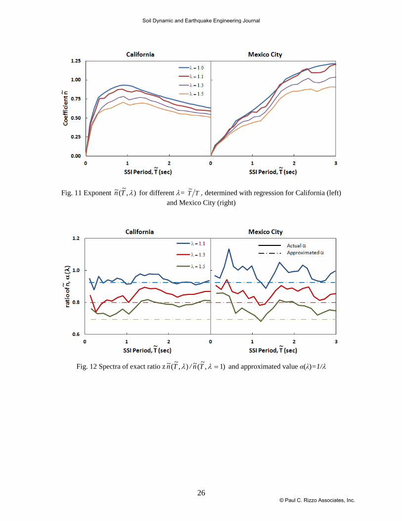
The exponent (T~ , λ) in (8), and similar ones for other values of λ, are plotted in Fig. 11,

which shows that is a decreasing function of λ, and vanishes for T~ = 0. This implies that

),(0,~ λµyC = C(0, λ), and since C(0, λ) = PGA /g, the condition that a ),(0,~ λµyC must be

equal to PGA /g is satisfied.

Since ),~(~ λTn decreases for increasing λ, (8) implies that for a prescribed µ , yC~ also

increases with λ, i.e., yC~ is larger for softer than for stiffer soils. To assess the effects of T~ and λ

on separately, it is useful to express the exponent ),~(~ λTn as the product:

),~(~ λTn = n(T~ ) α(λ) (10)

in which n(T~ ) is the limit of ),~(~ λTn for a fixed-base system (λ = 1), evaluated at the SSI

period T~ . The factor α(λ) accounts for the effect of λ. We use the results of Fig. 11 to obtain

α(λ), by dividing ),~(~ λTn by )1,~(~ =λTn . Observing that this ratio varies weakly with T~ , α(λ)

can be approximated as:

( ) ( )( ) λλ

λλα

11,~~

,~~≈

==

TnTn , 1 ≤ λ ≤ 1.5, (11)

The actual ratio α(λ) and its approximation 1/λ are shown in Fig. 12. Almost everywhere the

latter is smaller than the former. Since a smaller α(λ) yields a higher seismic coefficient, 1/λ

provides a conservative value of the seismic coefficient. With the approximations (9), (10) and

(11), the expression (8) for yC~ becomes:

( ) ( )( )λµ

λµ,,~~

~,,~~

TRTC

TyC = (12)

where

( )

=

λµλµ

1~

,,~~ TnTR (13)

Substituting from (1), this expression may be also written as:



10

( ) ( )

−=

λλ

µ

µλµ 1~

,~,,~~

Tn

TCTyC (14)

This expression indicates that in order to obtain the seismic coefficient of the SSI system with

a natural period T~ and a period elongation ratio λ it suffices to divide the seismic coefficient of a

rigid-base structure with the natural period T~ and a mean ductility demand µ by the factor

−

λλ

µ1~Tn

.

To assess the accuracy of (14) for determining the seismic coefficient, yC~ , of the SSI system

with a target ductility demand µt, we first obtained the “exact” value of yC~ from regression of

nonlinear analyses results obtained directly from the solution of the governing equations of the

system. Then we applied (14) to estimate yC~ . Results of the two approaches for different values

of λ and µt are plotted in Fig. 13. The difference between the two sets of curves is small. This

means that (14) provides a satisfactory estimate of yC~ for the two ensembles of earthquake

records, for all values of the target ductility, and for all ratios TT~ .

It is of considerable practical interest that (14) holds for the two very different sets of

earthquake records considered in this study. This indicates that a simple rule of the type embodied

in (11) might be applicable to other seismic regions.

As a further test of the accuracy of (14), Fig. 14 shows the actual mean ductility demand µ of

SSI systems whose strength is evaluated from this expression, for a prescribed target ductility μt.

The values of µ are in close agreement with μt, except for long period systems and λ = 1.5 in

Mexico City. In practice, such a large interaction ratio is unlikely for long period structures,

because they are built on pile foundations, which tend to increase the relative stiffness between

the foundation and the structure.

6.2 Structural Displacements

Having established a simple procedure for determining the SSI seismic design coefficient yC~ ,

and thereby the yield displacement via (6), the maximum mean relative displacement of the

inelastic superstructure, maxu , can be approximated consistently within this approach as the yield

displacement times the mean ductility demand µ . That is:



11

( )2π

µµ

2~

2

maxgTC

uu yy

⋅== (15)

With maxu known, the mean total displacement, totalu , of the mass of the structure with

respect to the free-field motion of the base can be estimated approximately as:

φhuuu xtotal ++= max (16)

xu is the mean relative horizontal displacement of the foundation with respect to the free-field

displacement and φ is the mean angle of rocking of the foundation. Using the assumption that

the foundation remains elastic, with horizontal and rocking stiffness kx and kφ, xu and φ are:

x

yx k

Vu

~= (17)

φ

φk

Vhh y

~2 ⋅= (18)

Substituting (13), (15) and (16) into (14), the total displacement becomes:

kV

kkh

kk

kVh

kV

kV

u y

xt

y

x

yyttotal

~~~~ 22

⋅++=

⋅++=

φφ

µµ (19)

Now, because yV~ /k = yu~ , the above equation can be rewritten as:

( )

⋅+++−=

φ

µk

khkkuuux

ytytotal

2

1~1~ (20)

From (2), the terms inside the second parenthesis are equal to the square of λ; thus:

( )1~ 2 −+= λµ tytotal uu (21)

Equation (21) allows one to compare the relative effect of the target ductility to that of the

flexibility of the soil on the total displacement of the structure. The ratio of the approximate mean

total relative displacement evaluated with (21) to the exact value obtained by solving the

nonlinear equations of motion has been calculated for different values of λ and μt. The results

presented in Fig. 15, indicate that the maximum difference between the approximate and exact

solutions is 10 percent and occurs for λ = 1.5 and µt = 5, for the Mexican records. For the

California records the discrepancy is less than 5 percent for any combination of λ and μt.

7. CONCLUDING REMARKS



12

In this study of the SSI response of inelastic structures to two very different sets of

earthquake records, we have first confirmed that for the simple linear systems considered in this

study, SSI mostly leads to a reduction of the mean response with respect to that of the

corresponding fixed-based structures. By contrast, a bilinear hysteretic structural behavior results

in an increase of the mean ductility demand with respect to that of the corresponding fixed-base

structure if the natural period of the system is smaller than the dominant period of the excitation

at the site, and in a decrease otherwise.

Based on these observations, we developed a simple procedure for estimating the SSI seismic

coefficient, yC~ , such that the ductility demand of the structure remains close to the target

ductility. In particular we derived an expression for yC~ as the product of the seismic coefficient

for the structure on a fixed-base structure divided by a factor that incorporates the SSI effects.

This result suggests that the seismic design coefficient can be determined from expression

(14). One only needs to replace the mean ductility demand µ by the target ductility, µt. In

practice, building codes stipulate a reduction factor R associated with the inelastic behavior of the

fixed-base structure. To incorporate SSI with our approach one would use a smaller reduction

factor ( )tTR µλ,,~~ equal to λλµ /)1)(~( −TntR .

The proposed approach can be used for rapidly assessing the importance of SSI effects on the

dynamic behavior of the building-foundation system, by comparing the seismic response

coefficient or, perhaps better yet, the resulting drift or peak structural displacement, with the

corresponding fixed-base quantities.

The results presented in this paper correspond to a structural aspect ratio, H/B = 2; we have

also analyzed SSI systems with H/B = 4, obtaining very similar qualitative results. The impact of

H/B is properly considered in the calculation of period elongation ratio λ. The proposed approach

has been developed for a particular class of SSI systems; while it is reasonable to expect that the

key equation (10) will apply to other foundation conditions, e.g., piles, and soil stratigraphy, the

procedure should be additionally verified before applying it to systems whose structural behavior

differs widely from the bilinear hysteretic considered here. It is also well to emphasize that only

inertial interaction has been considered in this study. Kinematic interaction should be included if

the dominant length of the incident waves is of the same order as the base (or depth) dimension of

the foundation.

ACKNOWLEDGMENTS



13

This research was partially supported by the National Science Foundation Division of

Engineering Education and Centers under grant 01-21989. The authors are grateful for this

support. We also thank the reviewers for their constructive comments. They were very helpful in

revising the paper.

REFERENCES

[1] ASCE, ASCE 7-10 Minimum Design Loads for Buildings and Other Structures, American Society of Civil Engineers, 2010.

[2] NTDF, “Normas Técnicas Complementarias para Diseño por Sismo”, Gaceta Oficial del Distrito Federal , Mexico City, Mexico, 2004.

[3] NEHRP, NEHRP Recommended Provisions for Seismic Regulations for New Buildings and Other Structures. Part 1 – Provisions 2009 Edition; FEMA 750 CD.

[4] Stewart JP, Kim S, Bielak J, Dobry R, and Power MS. Revisions to Soil-Structure Interaction Procedures in NEHRP Design Provisions. Earthquake Spectra 2003; 19(3): 677-696.

[5] Bielak J. Earthquake response of building-foundation systems. Technical Report: CaltechEERL:1971.EERL-71-04, California Institute of Technology 1971; http://caltecheerl.library.caltech.edu/197/00/7104.pdf

[6] Jennings, PC, and Bielak, J. Dynamics of Building-Soil Interaction. Bull. Seism. Soc. Am.1973; 63 (1): 9-48.

[7] Veletsos AS and Meek JW. Dynamic behavior of building-foundation systems Earthquake Engineering and Structural Dynamics 1974; 3(2): 121-138.

[8] Luco JE. Linear Soil Structure Interaction, in Seismic Safety Margins Research Program (Phase I), U.S. Nuclear Regulatory Commission, Washington D.C., 1980.

[9] Roesset JM. “A review of soil-structure interaction,” in Soil-structure interaction: The status of current analysis methods and research, J. J. Johnson, ed., Rpt. No. NUREG/CR-1780 and UCRL-53011, U.S. Nuclear Regulatory Com., Washington DC, and Lawrence Lab., Livermore, CA., 1980.

[10] Isenberg J. Interaction between soil and nuclear reactor foundation during earthquakes. USAEC Report, ORO-3822-5, Agbabian-Jacobsen Associates, Los Angeles, California 1970.

[11] Minami T. Elastic-plastic earthquake response of soil-building systems. Proc. Fifth World Conference Earthquake Engineering, Rome, Italy 1973; 2080-2083.

[12] Kobori T, Minai R, and Inoue Y. On earthquake response of elasto-plastic structure considering ground characteristics. Proc. Fourth World Conference Earthquake Engineering, 3, Santiago, Chile, 1969: 117-132.

[13] Inoue Y, Kawano M, and Maeda Y. Dynamic response of nonlinear soil-structure systems. Technology Reports of the Osaka University1974; 24: 803-825.

[14] Veletsos AS and Verbic B. Dynamics of elastic and yielding structure-foundation systems. Proc. Fifth World Conference Earthquake Engineering, Rome, Italy 1973; 2610-2613.

[15] Bielak J. Dynamic Response of Non-Linear Building-Foundation Systems. Earthquake Engineering and Structural Dynamics 1978; 6, 17-30.

[16] Bazán-Zurita E, Díaz-Molina I, Bielak J, and Bazán-Arias NC. Probabilistic seismic response of inelastic building foundation systems. Proc. 10th World Conf. on Earthq. Engineering, Madrid, Spain1992; 1559-1565.

[17] Rodríguez M and Montes R. Seismic response and damage analysis of buildings supported on flexible soils, Earthq Engineering & Struct. Dyn 2000; 29: 647-665



http://caltecheerl.library.caltech.edu/197/00/7104.pdf�

14

[18] Mylonakis G. and Gazetas G. Seismic Soil-Structure Interaction: Beneficial or Detrimental? Journal of Earthquake Engineering 2000; 4(3): 377-401

[19] Avilés J and Pérez-Rocha LE. Soil-structure interaction in yielding systems. Earthquake Engineering and Structural Dynamics 2003; 32: 1749-1771.

[20] Jarernprasert S, Bazan E, and Bielak J. An Inelastic-Based Approach for Seismic Design Spectra. Journal of Structural engineering 2006; 132;, 1284-1292.

[21] Jarernprasert S. An inelastic design approach for asymmetric structure-foundation systems. Ph.D. Dissertation, Carnegie Mellon University, Pittsburgh, PA, 2005.

[22] Arias A and Husid R. Influencia del amortiguamiento sobre la respuesta de estructuras sometidas a temblor. (In Spanish), Rev. IDIEM 1962; Vol 1: 219-228.

[23] Gazetas G. (1991). Foundation Vibration. Foundation Engineering Handbook. H.-Y. Fang. Van Nostrand Reinhold, New York: Chapter 15.

[24] Avilés J and Pérez-Rocha LE 1996. Evaluation of interaction effects on the system period and the system damping due to foundation embedment and layer depth. Soil Dynamics and Earthquake Engineering 1996; 15(1): 11-27.

[25] Chopra AK. Dynamics of Structures, Theory and Applications to Earthquake Engineering, Prentice Hall, Upper Saddle River, New Jersey, 1995.



15

APPENDIX A Symbol Description

B Base dimension of the foundation C Pseudo-elastic spectrum of fixed-base system C~ Pseudo-elastic spectrum of SSI system

eC Average Elastic spectrum of fixed-base system

Cv Foundation horizontal viscous damping Cφ Foundation rocking viscous damping

yC~ Inelastic spectrum of SSI system Cy Inelastic spectrum of fixed-base system D Soil hysteretic damping g Gravitational acceleration H Actual height of super structure h Equivalent height of fixed-base system k Translational stiffness of fixed-base system kv Translational stiffness of foundation kφ Rocking stiffness of foundation m Mass of super structure m0 Mass of foundation n Inelastic modification factor of fixed-base system n~ Inelastic modification factor of SSI system PGA Average peak ground acceleration r Equivalent radius of base dimension of the foundation R Fixed-base inelastic reduction factor R~ SSI inelastic reduction factor T~ SSI period T Fixed-base period umax Maximum relative displacement

maxu Average maximum relative displacement

totalu Average total displacement

xu Average translational displacement of foundation uy Fixed-base yielding displacement

yu~ SSI yielding displacement Vs Soil shear wave velocity

eV Average fixed-base elastic base shear Vy Fixed-base yield base shear

yV~ SSI yield base shear W Weight of super structure

α Exponent of SSI inelastic modification factor β~ Total SSI effective damping ratio βο SSI effective damping ratio from foundation interaction λ Ratio of SSI period respect to Fixed-base period µ Ductility demand μt Target ductility



16

µ Average ductility demand φ Average rotation of foundation



17

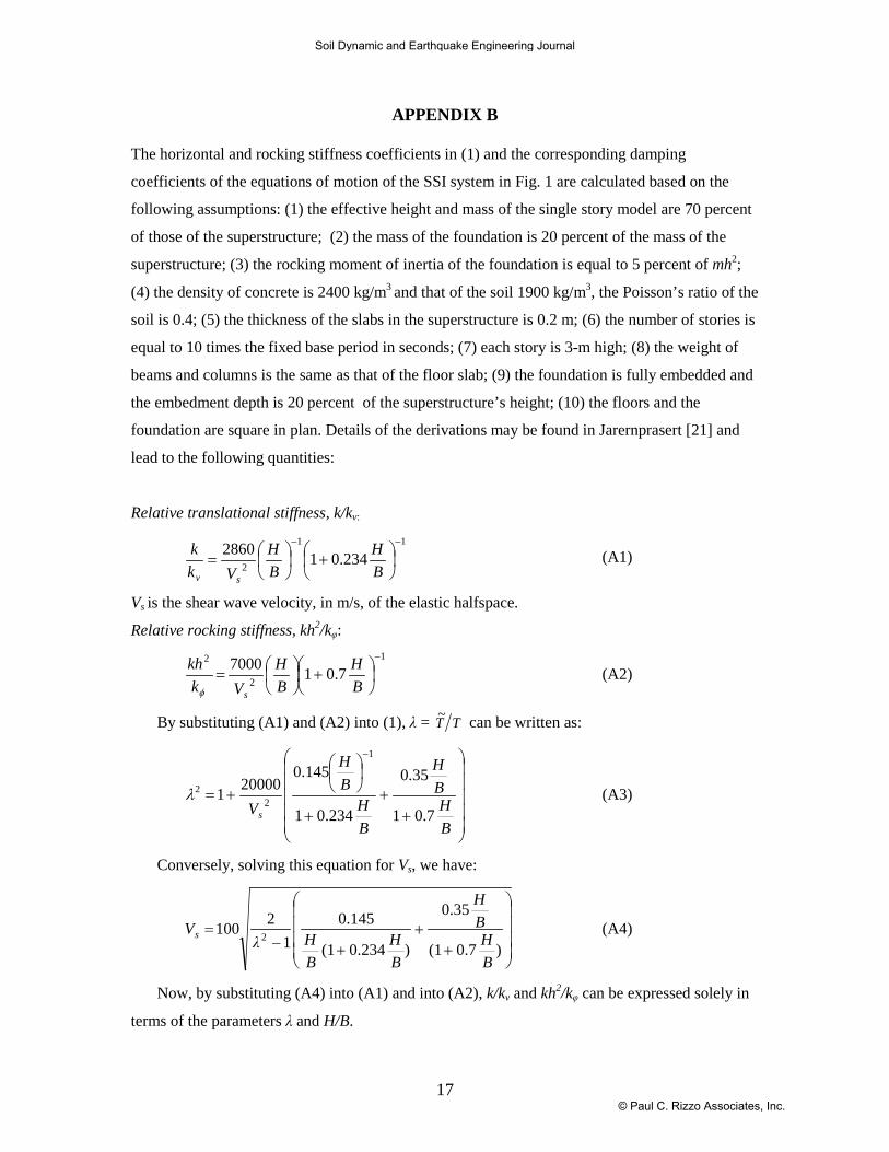
APPENDIX B

The horizontal and rocking stiffness coefficients in (1) and the corresponding damping

coefficients of the equations of motion of the SSI system in Fig. 1 are calculated based on the

following assumptions: (1) the effective height and mass of the single story model are 70 percent

of those of the superstructure; (2) the mass of the foundation is 20 percent of the mass of the

superstructure; (3) the rocking moment of inertia of the foundation is equal to 5 percent of mh2;

(4) the density of concrete is 2400 kg/m3 and that of the soil 1900 kg/m3, the Poisson’s ratio of the

soil is 0.4; (5) the thickness of the slabs in the superstructure is 0.2 m; (6) the number of stories is

equal to 10 times the fixed base period in seconds; (7) each story is 3-m high; (8) the weight of

beams and columns is the same as that of the floor slab; (9) the foundation is fully embedded and

the embedment depth is 20 percent of the superstructure’s height; (10) the floors and the

foundation are square in plan. Details of the derivations may be found in Jarernprasert [21] and

lead to the following quantities:

Relative translational stiffness, k/kv:

11

2 234.012860 −−

+

=

BH

BH

Vkk

sv (A1)

Vs is the shear wave velocity, in m/s, of the elastic halfspace.

Relative rocking stiffness, kh2/kφ:

1

2

2

7.017000 −

+

=

BH

BH

Vkkh

sφ

(A2)

By substituting (A1) and (A2) into (1), λ = TT~ can be written as:

++

+

+=

−

BH

BH

BH

BH

Vs 7.01

35.0

234.01

145.0200001

1

22λ (A3)

Conversely, solving this equation for Vs, we have:

++

+−=

)0.7(1

0.35

)0.234(1

0.1451

2100 2

BH

BH

BH

BHλ

Vs (A4)

Now, by substituting (A4) into (A1) and into (A2), k/kv and kh2/kφ can be expressed solely in

terms of the parameters λ and H/B.



18

Damping

β0 in (2) can be related to the coefficients cv and cφ of the two viscous dampers used in the SSI

system shown in Fig. 2 as follows:

+

=

−

φ

φπβkkh

hC

kkC

TT

kT vv

2

2

23

0 ~ (A5)

Using (A5) and the formulas in Gazetas (1991), we obtain:

DTTTk

kkh

kk

TTkT

C v

v

v

+

+

=~

~

22

3

0

πα

πβ

φ

(A6)

DTT

hTk

kkh

kk

TTkT

hC

v

+

+

=~

~

222

3

0

2 πψ

πβ

φ

φ

φ (A7)

D is the fraction of linear hysteretic damping in the soil, taken to be 0.05, and ψ is given by:

2

2410367.0

= −−

BHTVx sψ (A8)



19

APPENDIX C

As an example of the individual calculations performed as the basic step for evaluating the

average ductility demand, µ , in this Appendix we describe the seismic response of a specific

inelastic structure excited by the SCT2990930.3 record from the Mexican database. The selected

structure has a fixed-base period T = 1.0 sec, 5% critical damping, and H/B = 2. The properties of

the SSI system were defined by the procedure described in Appendix B to yield an SSI period of

1.3 sec. Both systems have a seismic coefficient of 0.95.

Figure C1 shows the strong segments of the relative displacements normalized by the yield

displacement of the structure, uy (the same for both the fixed-base and the SSI cases.) The

properties of the selected system and the peak values of the normalized relative displacement with

and without interaction are summarized in Table C1. These peak values are the ductility

demands.

Table C1. Comparison of dynamic properties and response of a selected case

Property Fixed-base structure

SSI system

Natural period (s) 1.0 1.3 Period elongation ratio, λ= T~ / Τ 1.0 1.3 Effective damping (%) 5 Code formula Peak relative displacement normalized with respect to yield displacement (also, ductility demand)

4.7 5.9

For this example, the ductility demand when SSI is considered is 26 percent larger than when SSI

is disregarded. By counting the response peaks in Fig. C1, it is apparent that the displacement of

the SSI system (λ = 1.3) exhibits fewer cycles than those of the fixed base structure because the

elongated natural period, T~ , dominates the seismic response.



20

Fig. 1 Mean elastic spectrum with 5% damping ratio and inelastic coefficients C and n for

accelerograms from California (left) and from Mexico City (right)

Fig. 2 Fixed-base and SSI systems: (a) Fixed-base system (b) Soil structure interaction system (c)

Hysteretic behavior



21

Fig. 3 Mean response spectra of elastic SSI systems for different λ = TT~ , in terms of the fixed-base period, T for California (left) and Mexico City (right)

Fig. 4 Mean response spectra of elastic SSI systems for different λ = TT~ , in terms of the SSI period, T~ , for California (left) and Mexico City (right)



22

Fig. 5 Inelastic mean seismic coefficient for different λ= TT~ , for a target ductility µt = 2, in terms of SSI period, T~ , for California (left) and Mexico City (right)

Fig. 6 Inelastic mean seismic coefficient for different λ= TT~ , for a target ductility demand µt = 4, as a function of SSI period, T~ for California (left) and Mexico City (right)



23

Fig. 7 Comparison of target ductilities (dotted lines) with mean ductility demands of SSI systems

designed with current code SSI provisions (solid lines), for λ = TT~ = 1.1, 1.3 and 1.5, for California (left) and Mexican records (right)



24

Fig. 8 Comparison of target ductility (dotted lines) with mean ductility demands for SSI systems

designed ignoring SSI (solid lines) for λ = TT~ = 1.1, 1.3, and 1.5, for California (left) and Mexican records (right)



25

Fig. 9 Variability of mean ductility demand µ with yield strength yC~ for systems with

λ = TT~ = 1.3 and prescribed fixed-base elastic periods, T, for California (left) and Mexico City (right)

Fig. 10 Unreduced Inelastic Spectra ),~(~ λTC for different λ= TT~ , determined by regression for

California (left) and Mexico City (right)



26

Fig. 11 Exponent ),~(~ λTn for different λ= TT~ , determined with regression for California (left) and Mexico City (right)

Fig. 12 Spectra of exact ratio z ),~(~ λTn / )1,~(~ =λTn and approximated value α(λ)=1/λ



27

Fig. 13 Comparison of “exact” and approximate seismic coefficients of SSI inelastic systems with

λ = TT~ = 1.1 to 1.5 from top to bottom, respectively, for California (left) and Mexico City (right)



28

Fig. 14 Mean response ductility demand of inelastic SSI structures designed via the proposed SSI

method (solid line) with λ = TT~ = 1.1, 1.3 and 1.5 from top to bottom, respectively, for Californian (left) and Mexican records (right)



29

Fig. 15 Ratio of mean maximum total displacement of SSI systems from (21) to the “exact” value from numerical integration, for Californian (left) and Mexican (right) records, for target ductility

µt between 2 and 5.

Fig. C1 Response of a selected structure to the Mexican SCT2990930 record



Documents

SEISMIC SOIL-STRUCTURE INTERACTION RESPONSE OF INELASTIC