Inelastic strain distribution and seismic radiation from ...people.tamu.edu/~bduan/Duan_2008JB005847.pdf · Inelastic strain distribution and seismic radiation from rupture of a fault

Inelastic strain distribution and seismic radiation from rupture

of a fault kink

Benchun Duan1 and Steven M. Day2

Received 3 June 2008; revised 25 September 2008; accepted 14 October 2008; published 30 December 2008.

[1] We extend an elastodynamic finite element method to incorporate off-fault plasticyielding into a dynamic earthquake rupture model. We simulate rupture for models offaults with a kink (a sharp change in fault strike), examining how off-fault plastic yieldingaffects rupture propagation, seismic radiation, and near-fault strain distribution. Wefind that high-frequency radiation from a kink can be reduced by strong plastic yieldingnear the kink. The reduction is significant above several Hz. When rupture propagatesaround the kink onto a less favorably stressed fault segment, plastic strain tends to localizeinto bands and lobes. Off-fault plastic yielding also significantly reduces heterogeneityof residual stresses around the kink following a dynamic event. The calculated plasticstrain distribution around the kink and the radiated pulse from the kink are nearly gridindependent over the range of element size for which computations are feasible. Wealso find that plastic strain can sometimes localize spontaneously during rupture along aplanar fault, in the absence of a discrete stress concentrator like the kink. In that case, anon-dimensional parameter T, characterizing the initial proximity of off-fault materialto its yield strength, determines whether plastic strain localizes into discrete bands or issmoothly distributed, with a large value of T promoting localization. However, in the casesof spontaneous localization, the details of the shear banding change with numericalelement size, indicating that the final plastic strain distribution is influenced byinteractions occurring at the shortest numerically resolvable scales. Off-fault plasticyielding also makes an important contribution to the cohesive zone at the advancing edgeof the rupture.

Citation: Duan, B., and S. M. Day (2008), Inelastic strain distribution and seismic radiation from rupture of a fault kink, J. Geophys.

Res., 113, B12311, doi:10.1029/2008JB005847.

1. Introduction

[2] It has long been recognized that an abrupt change inearthquake rupture speed results in high-frequency radiation[Madariaga, 1977]. Observations and theoretical studieshave shown that a fault kink can cause abrupt changes inrupture speed [e.g., King and Nabelek, 1985; Bouchon andStreiff, 1997; Aochi et al., 2000; Duan and Oglesby, 2005;Ely et al., 2008]. More recently, an analysis of seismicradiation from a kink on an antiplane fault performed byAdda-Bedia and Madariaga [2008] shows that rupturethrough a fault kink radiates a step function in particlevelocities. A velocity step entails strong high-frequencyradiation to the far field, with displacement spectrumproportional to f�2 (f is frequency). This analysis of thekink contribution to seismic radiation assumes, of course,that deformation in the medium surrounding the fault ispurely elastic.

[3] Detailed geological measurements on exhumed faultzones, such as the Punchbowl fault in southern California,have shown that the core of a fault, i.e., the zone with athickness of cm to tens of cm that accommodates most ofslip, is surrounded by a zone of cataclastic material with athickness of few meters and a broader damage zone that isseveral hundred meter wide [e.g., Chester and Chester,1998; Ben-Zion and Sammis, 2003; Chester et al., 2004].Trapped-wave studies [e.g., Li et al., 1994; Ben-Zion et al.,2003] reveal a low-velocity zone with a width of tens tohundreds of meters around the active faults in Californiaand Turkey. A new observation of fault guided PSV-wavesat SAFOD (San Andreas Fault Observatory at Depth)supports the hypothesis that the low-velocity fault zonescan extend deep into the seismogenic crust [Ellsworth andMalin, 2006]. These observations suggest that slip during anearthquake rupture is localized on the core of a fault, and isaccompanied by inelastic deformation distributed in a zonesurrounding the core.[4] Theoretical analyses on the stress field near the tip of

a steadily propagating rupture suggest that stresses elasti-cally predicted near the rupture front can be large enough tocause failure of off-fault material, based on a Coulombfailure criterion, particularly for propagation speed near the

JOURNAL OF GEOPHYSICAL RESEARCH, VOL. 113, B12311, doi:10.1029/2008JB005847, 2008ClickHere

for

FullArticle

1Department of Geology and Geophysics, Texas A&M University,College Station, Texas, USA.

2Department of Geological Sciences, San Diego State University, SanDiego, California, USA.

Copyright 2008 by the American Geophysical Union.0148-0227/08/2008JB005847$09.00

B12311 1 of 19

http://dx.doi.org/10.1029/2008JB005847

theoretical limiting speed for a sharp crack (e.g., theRayleigh speed for mode II rupture) [Poliakov et al.,2002; Rice et al., 2005]. These studies indicate the likelyimportance of off-fault inelastic response for models ofrupture behavior and ground motion excitation. Andrews[2005] has modeled this inelastic response on planar faults,using Mohr-Coulomb elastoplasticity. He has shown that, insuch models, energy loss off the fault is proportional topropagation length (in 2D), and is much larger than energyloss on the fault. Templeton and Rice [2008] have used thesimilar Drucker-Prager elastoplastic model to study theextent and distribution of off-fault plasticity during seismicrupture on a planar fault. Numerical simulations by Andrewset al. [2007] have shown that nonlinear material responsemay significantly affect model predictions of near-faultground motion.[5] In this study, we model rupture on both planar and

kinked faults, using a simple (slip-weakening) friction law,in 2D (mode II, in-plane motion). We retain the approach byAndrews [2005], treating off-fault material as a Mohr-Coulomb elastoplastic solid, with post-yielding behaviorgoverned by a non-associative flow rule. Through compar-isons with elastodynamic simulations for the same geome-tries, we examine effects of yielding on rupture propagation,strain distribution, and seismic radiation.

2. Method

[6] We modify an elastodynamic finite element methodcode EQdyna [Duan and Oglesby, 2006] to allow the off-fault material to yield when the stress state reaches aCoulomb yield criterion [Scholz, 2002; Andrews, 2005].

2.1. EQdyna: An Explicit Finite Element Method(FEM) for Elastoplastic Dynamic Analysis

[7] To perform elastoplastic dynamic analysis, the ele-ment stress cannot be calculated from displacement, as itcan in elastodynamic analysis. Rather, the element stressmust be updated from the previous time step value byintegrating the stress rate. The stress rate can be computedfrom the element nodal velocity. The general structure ofEQdyna [Duan and Oglesby, 2006] does not require change.The major modifications involve only the element stresscalculation and implementation of the stiffness-proportionalRayleigh damping at the element level.[8] From the element point of view, the internal force for

elastic analysis can be computed by [e.g., Hughes, 2000]

f e ¼ kede ¼ 4jBTDBde; ð1Þ

where f e, de, ke are the nodal force vector, the displacementvector, and the element stiffness matrix, respectively, j is theJacobin determinant, and B and D are, respectively, thestrain-displacement matrix and the constitutive matrix withstandard definition in the FEM literature [e.g., Hughes,2000]. Equation (1) is based upon one-point GaussianQuadrature, which (in 2D) accounts for the pre-factor of 4appearing in (1). In the code, one does not have to calculatethe element stiffness matrix. Rather, the multiplication onthe right hand of equation (1) can be performed from right

to left. In this point of view, the element strain and stressvectors at the integration point are

ee ¼ Bde

se ¼ Dee; ð2Þ

where, the superscript e denotes ‘‘element’’, indicating theelement point of view of the quantities. In elastic analysis,one does not need to explicitly calculate the element strainand stress if they are not required for analysis. However, theelement stress is required in elastoplastic analysis to assessthe Coulomb yield criterion. We remark that the elementstress is calculated at the Gaussian quadrature point (thecenter of the element), while the internal force is evaluatedat the element nodes.[9] For elastoplastic dynamic analyses, we require the

elastic stress increments (which may be subsequently mod-ified by the yield condition) at each time step. One canevaluate them from element strain rate and stress rate at theintegration point, using the time derivatives of (2),

_ee ¼ Bve

_se ¼ D _ee; ð3Þ

where overdot represents the time derivative, and ve is thevelocity vector. Then the element stress at the time step n + 1can be updated from the value of the previous time stepn through time integration, approximated by

senþ1 ¼ se

n þ _seDt; ð4Þ

where Dt is the dynamic simulation time step. This is thetrial element stress and may be altered if plastic yieldingoccurs. In this update scheme, velocity, strain rate, andstress rate are evaluated at the time (n + 1/2) Dt. Then theinternal nodal force vector (at the element level) at the timestep n + 1 can be calculated as

f enþ1 ¼ 4jBTsenþ1: ð5Þ

[10] In addition to the above modification in the internalforce calculation, the implementation of the stiffness-proportional Rayleigh damping [e.g., Hughes, 2000] alsoneeds to be revised. In elastic analyses, one can easilyimplement the damping by adding a correction vector qve tothe displacement vector de before calculating the internalforce [Hughes, 2000; Duan and Oglesby, 2006]. Here, q isthe damping coefficient. In elastoplastic analyses, thisdamping force needs to be calculated separately from theinternal force. Using the above notation, one can calculatethe element damping force vector at the time step n + 1 fromthe stress rate at the time (n + 1/2) Dt as

fdampnþ1 ¼ 4jqBT _se: ð6Þ

[11] In the new version of the code EQdyna, we still usethe traction-at-split-node (TSN) treatment for the faultboundary [Andrews, 1999]. In this method, a given faultplane node is split into two halves, which interact throughtraction acting on the interface between them. The calculated

B12311 DUAN AND DAY: KINK RADIATION AND STRAIN LOCALIZATION

2 of 19

B12311

fault-plane nodal tractions (shear and normal components)represent averages over adjacent element edges, that is, eachis a nodal force divided by an effective element-edge area;the fault boundary conditions are enforced for these aver-aged quantities. We adopt the formulation given by Day etal. [2005] in the new version, which provides a consistenttreatment for fault behavior (at a given pair of split nodes) atall times, including pre-rupture, rupture initiation, arrest ofsliding, and possible reactivation and arrest of sliding. Inthis work, rupture is artificially initiated from the uniformstress state by prescribing stress drops on the fault behind arupture front that propagates at a fixed speed (2000 m/s,which is two thirds of the shear wave speed in the models ofthis study). This artificial initiation is enforced within anucleation zone with half length of L0. Beyond this zone,rupture propagates spontaneously. This initiation scheme issimilar to that used by Andrews [2005] for similar calcu-lations with nonelastic off-fault response.

2.2. Off-Fault Elastoplastic Material Behavior

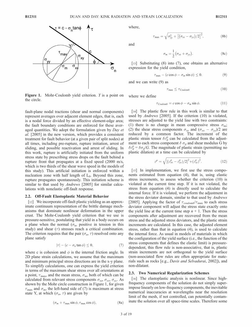
[12] We incorporate off-fault plastic yielding as an approx-imate continuum representation of the brittle damage mech-anisms that dominate nonlinear deformation in the uppercrust. The Mohr-Coulomb yield criterion that we use ispressure-sensitive, postulating that yield in a body occurs ona plane when the normal (sn, positive in tension in thisstudy) and shear (t) stresses reach a critical combination.The criterion requires that the pair (sn, t) resolved onto anyplane satisfy

tj j � c� sn tanfð Þ � 0; ð7Þ

where c is cohesion and f is the internal friction angle. In2D plane strain calculations, we assume that the maximumand minimum principal stress directions are in the x-y plane.To simplify calculations, one can express the yield criterionin terms of the maximum shear stress over all orientations ata point, tmax, and the mean stress, sm, both of which can becalculated from relevant stress components sxy, sxx, syy. Asshown by the Mohr circle construction in Figure 1, for giventmax and sm, the left-hand side of (7) is maximum at stressstate Y, at which (sn, t) are given by

sm þ tmax sinf; tmax cosfð Þ; ð8aÞ

where,

tmax ¼ffiffiffiffiffiffiffiffiffiffiffiffiffiffiffiffiffiffiffiffiffiffiffiffiffiffiffiffiffiffiffiffiffiffiffiffiffiffiffiffiffiffiffiffiffis2xy þ sxx � syy

� �=2

� �2q; ð8bÞ

and

sm ¼ 1

2sxx þ syy

� �: ð8cÞ

[13] Substituting (8) into (7), one obtains an alternativeexpression for the yield condition,

tmax � c cosf� sm sinfð Þ � 0: ð9Þ

and we can write (9) as

tmax � tCoulomb ð10Þ

where we define

tCoulomb ¼ c cosf� sm sinf: ð11Þ

[14] The plastic flow rule in this work is similar to thatused by Andrews [2005]. If the criterion (10) is violated,stresses are adjusted to the yield line with two constraints:(1) there is no change in mean compressive stress sm;(2) the shear stress components sxy and (sxx � syy)/2 arereduced by a common factor. The increment of theplastic strain tensor deij

p can be calculated from the adjust-ment to each stress component d sij and shear modulus G bydeij

p = dsij/G. The magnitude of plastic strain (permitting noplastic dilation) at a time can be calculated by

ep ¼ffiffiffiffiffiffiffiffiffiffiffiffiffiffiffiffiffiffiffiffiffiffiffiffiffiffiffiffiffiffiffiffiffiffiffiffiffiffiffiffiffiffiffiffiffiepxx � epyyð Þ=2½ 2þ epxyð Þ2

q: ð12Þ

[15] In implementation, we first use the stress compo-nents estimated from equation (4), that is, using elasticstress increments, to assess whether the criterion (10) isviolated at the current time step. If it is not violated, thestress from equation (4) is directly used to calculate theinternal force. If it is violated, we perform the adjustment inthe stress deviator domain, similar to that used by Andrews[2005]. Applying the factor of tcoulomb/tmax to each stressdeviator component will adjust the stress state exactly ontothe yield line at the current time step n + 1. Then the stresscomponents after adjustment are recovered from the meanstress and the adjusted stress deviators, and the plastic strainincrements are calculated. In this case, the adjusted elementstress, rather than that in equation (4), is used to calculatethe internal force. As usual in models of materials in whichthe configuration of the yield surface (i.e., the function of thestress components that defines the elastic limit) is pressure-dependent, this flow rule is non-associative, that is, plasticstrain increments are not orthogonal to the yield surface(non-associated flow rules are often appropriate for mate-rials such as rocks [e.g., Davis and Selvadurai, 2002]), andnon-dilatant.

2.3. Two Numerical Regularization Schemes

[16] The elastoplastic analysis is nonlinear. Since high-frequency components of the solution do not simply super-impose linearly on low-frequency components, the inevitablenumerical inaccuracies at wavelengths near the resolutionlimit of the mesh, if not controlled, can potentially contam-inate the solution over all space-time scales. Therefore some

Figure 1. Mohr-Coulomb yield criterion. Y is a point onthe circle.


3 of 19

B12311

form of numerical regularization is usually necessary tosuppress solution components with spatial scale near thatresolution limit. We apply two schemes to regularizecalculations in the code: one is stiffness-proportional Ray-leigh damping; the other is Maxwellian viscoplasticity(time-dependent relaxation of the stress adjustment). Theformer introduces a Q (seismic quality factor, which charac-terizes the rate of decay of seismic waves) that is inverselyproportional to frequency, and therefore selectively dampswavelengths (l) near the resolution limit of the numericalmesh. The damping parameter q can be specified through anon-dimensional parameter b, such that q = bDt, orequivalently,

q ¼ baDx=vp: ð13Þ

where Dx is the minimum element dimension, a is theCourant-Friedrich-Lewy (CFL) number and Vp is the P wavevelocity. Then holding b fixed while the mesh is refined (atfixed CFL number) has the effect of shifting the absorptionband such that Q is unchanged as a function of l/Dx.Alternatively, one can hold q itself fixed to keep theabsorption band invariant as a function of l.[17] The second scheme, viscoplasticity, was used by

Andrews [2005] to regularize elastoplastic rupture simula-tions. In this scheme, the abrupt relaxation of the trial stress(4) is replaced by a smoothed relaxation with some expo-nential decay time Tv. That is, the stress adjustment factortcoulomb/tmax is replaced by {1 � (1 � tcoulomb/tmax)[1 �exp (�Dt/Tv)]}. We remark that a smaller Tv results in fasterrelaxation of the trial stress to the yield surface and thuscauses stronger off-fault plastic yielding that in turn leads toslower rupture propagation.[18] Both numerical parameters b and Tv have the

intended effect of removing poorly-resolved short-wave-

length features from the solution, and ideally we would likethe solution to be relatively insensitive to their precisevalues. Values of b of order 0.1 have been found effectivein reducing short-wavelength noise in elastodyanamic rup-ture simulations [Day et al., 2005; Duan and Oglesby, 2006,2007; Dalguer and Day, 2007]. Values of Tv of order Dx/Vs

(with Vs the S wave speed) were successfully used byAndrews [2005] to reduce short-wavelength noise in elasto-plastic rupture simulations.

2.4. Code Verification: Revisiting the Modelby Andrews

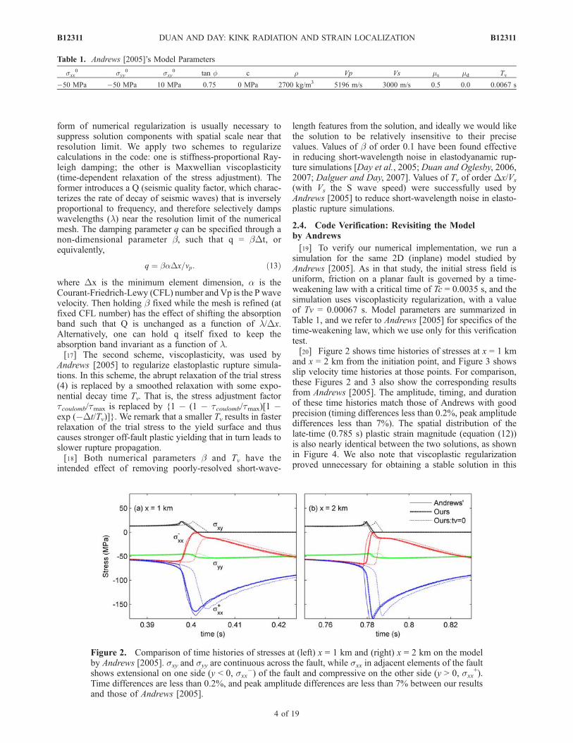
[19] To verify our numerical implementation, we run asimulation for the same 2D (inplane) model studied byAndrews [2005]. As in that study, the initial stress field isuniform, friction on a planar fault is governed by a time-weakening law with a critical time of Tc = 0.0035 s, and thesimulation uses viscoplasticity regularization, with a valueof Tv = 0.00067 s. Model parameters are summarized inTable 1, and we refer to Andrews [2005] for specifics of thetime-weakening law, which we use only for this verificationtest.[20] Figure 2 shows time histories of stresses at x = 1 km

and x = 2 km from the initiation point, and Figure 3 showsslip velocity time histories at those points. For comparison,these Figures 2 and 3 also show the corresponding resultsfrom Andrews [2005]. The amplitude, timing, and durationof these time histories match those of Andrews with goodprecision (timing differences less than 0.2%, peak amplitudedifferences less than 7%). The spatial distribution of thelate-time (0.785 s) plastic strain magnitude (equation (12))is also nearly identical between the two solutions, as shownin Figure 4. We also note that viscoplastic regularizationproved unnecessary for obtaining a stable solution in this

Table 1. Andrews [2005]’s Model Parameters

sxx0 syy

0 sxy0 tan f c r Vp Vs ms md Tv

�50 MPa �50 MPa 10 MPa 0.75 0 MPa 2700 kg/m3 5196 m/s 3000 m/s 0.5 0.0 0.0067 s

Figure 2. Comparison of time histories of stresses at (left) x = 1 km and (right) x = 2 km on the modelby Andrews [2005]. sxy and syy are continuous across the fault, while sxx in adjacent elements of the faultshows extensional on one side (y < 0, sxx

�) of the fault and compressive on the other side (y > 0, sxx+).

Time differences are less than 0.2%, and peak amplitude differences are less than 7% between our resultsand those of Andrews [2005].


4 of 19

B12311

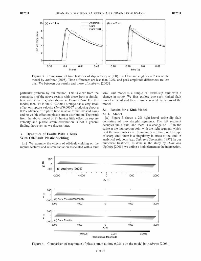
particular problem by our method. This is clear from thecomparison of the above results with those from a simula-tion with Tv = 0 s, also shown in Figures 2–4. For thismodel, then, Tv in the 0–0.00067 s range has a very smalleffect on rupture velocity (Tv of 0.00067 producing about a0.7% advance of rupture time relative to the inviscid case)and no visible effect on plastic strain distribution. The resultfrom the above model of Tv having little effect on rupturevelocity and plastic strain distribution is not a generalfinding, however, as we discuss later.

3. Dynamics of Faults With a KinkWith Off-Fault Plastic Yielding

[21] We examine the effects of off-fault yielding on therupture features and seismic radiation associated with a fault

kink. Our model is a simple 2D strike-slip fault with achange in strike. We first explore one such kinked faultmodel in detail and then examine several variations of themodel.

3.1. Results for a Kink Model

3.1.1. Model[22] Figure 5 shows a 2D right-lateral strike-slip fault

consisting of two straight segments. The left segmentoccupies the x axis, and there is a change of 10� in thestrike at the intersection point with the right segment, whichis at the coordinates x = 10 km and y = 0 km. For this typeof sharp kink, there is a singularity in stress at the kink inanalytical solutions [e.g., Tada and Yamashita, 1997]. In ournumerical treatment, as done in the study by Duan andOglesby [2005], we define a kink element at the intersection.

Figure 3. Comparison of time histories of slip velocity at (left) x = 1 km and (right) x = 2 km on themodel by Andrews [2005]. Time differences are less than 0.2%, and peak amplitude differences are lessthan 7% between our results and those of Andrews [2005].

Figure 4. Comparison of magnitude of plastic strain at time 0.785 s on the model by Andrews [2005].


5 of 19

B12311

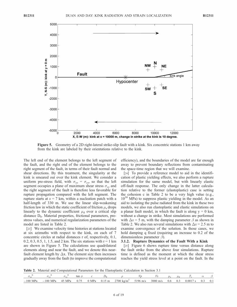
The left end of the element belongs to the left segment ofthe fault, and the right end of the element belongs to theright segment of the fault, in terms of their fault normal andshear directions. By this treatment, the singularity at thekink is smeared out over the kink element. We consider auniform pre-stress field, with sxx = syy, so that the leftsegment occupies a plane of maximum shear stress sxy andthe right segment of the fault is therefore less favorable forrupture propagation compared with the left segment. Therupture starts at x = 7 km, within a nucleation patch with ahalf-length of 330 m. We use the linear slip-weakeningfriction law in which the static coefficient of friction ms dropslinearly to the dynamic coefficient md over a critical slipdistance D0. Material properties, frictional parameters, pre-stress values, and numerical regularization parameters of themodel are listed in Table 2.[23] We examine velocity time histories at stations located

at six azimuths with respect to the kink, on each of 7concentric circles at radial distances r of, respectively, 0.1,0.2, 0.3, 0.5, 1, 1.5, and 2 km. The six stations with r = 1 kmare shown in Figure 5. The calculations use quadrilateralelements along and near the fault, and we denote this near-fault element length by Dx. The element size then increasesgradually away from the fault (to improve the computational

efficiency), and the boundaries of the model are far enoughaway to prevent boundary reflections from contaminatingthe space-time region that we will examine.[24] To provide a reference model to aid in the identifi-

cation of plastic yielding effects, we also perform a rupturesimulation for the same model, but with linearly elasticoff-fault response. The only change in the latter calcula-tion relative to the former (elastoplastic) case is settingthe cohesion c in Table 2 to be a very high value (e.g.,1030 MPa) to suppress plastic yielding in the model. As anaid to isolating the pulse radiated from the kink in these twomodels, we also run elastoplastic and elastic simulations ona planar fault model, in which the fault is along y = 0 km,without a change in strike. Most simulations are performedwith Dx = 5 m, with the damping parameter b as shown inTable 2. We also run several simulations with Dx = 2.5 m toexamine convergence of the solution. In those cases, wehold damping q fixed (requiring an increase to 0.2 of thedimensionless parameter b).3.1.2. Rupture Dynamics of the Fault With a Kink[25] Figure 6 shows rupture time versus distance along

the fault strike from the above four simulations. Rupturetime is defined as the moment at which the shear stressreaches the yield stress level at a point on the fault. In the

Figure 5. Geometry of a 2D right-lateral strike-slip fault with a kink. Six concentric stations 1 km awayfrom the kink are labeled by their orientations relative to the kink.

Table 2. Material and Computational Parameters for the Elastoplastic Calculation in Section 3.1

sxx0 syy

0 sxy0 tan f c D0 r Vp Vs ms md Tv a b

�100 MPa �100 MPa 45 MPa 0.75 0 MPa 0.15 m 2700 kg/m3 5196 m/s 3000 m/s 0.6 0.3 0.0017 s 0.3 0.1


6 of 19

B12311

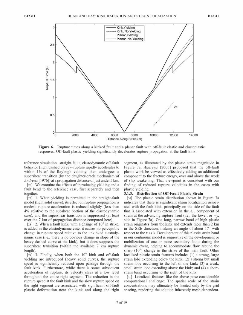
reference simulation–straight-fault, elastodynamic off-faultbehavior (light dashed curve)–rupture rapidly accelerates towithin 1% of the Rayleigh velocity, then undergoes asupershear transition (by the daughter-crack mechanism ofAndrews [1976]) at a propagation distance of just under 5 km.[26] We examine the effects of introducing yielding and a

fault bend to the reference case, first separately and thentogether.[27] 1. When yielding is permitted in the straight-fault

model (light solid curve), its effect on rupture propagation ismodest: rupture acceleration is reduced slightly (less than4% relative to the subshear portion of the elastodynamiccase), and the supershear transition is suppressed (at leastover the 7 km of propagation distance computed here).[28] 2. When a fault kink, with a change of 10� in strike,

is added in the elastodynamic case, it causes no perceptiblechange in rupture speed relative to the unkinked elastody-namic case (i.e., there is no obvious change in slope of theheavy dashed curve at the kink), but it does suppress thesupershear transition (within the available 7 km rupturelength).[29] 3. Finally, when both the 10� kink and off-fault

yielding are introduced (heavy solid curve), the rupturespeed is significantly reduced upon passage through thefault kink. Furthermore, while there is some subsequentacceleration of rupture, its velocity stays at a low levelthroughout the entire right segment. The reduction in therupture speed at the fault kink and the slow rupture speed onthe right segment are associated with significant off-faultplastic deformation near the kink and along the right

segment, as illustrated by the plastic strain magnitude inFigure 7a. Andrews [2005] proposed that the off-faultplastic work be viewed as effectively adding an additionalcomponent to the fracture energy, over and above the workof slip weakening. That viewpoint is consistent with ourfinding of reduced rupture velocities in the cases withplastic yielding.3.1.3. Distribution of Off-Fault Plastic Strain[30] The plastic strain distribution shown in Figure 7a

indicates that there is significant strain localization associ-ated with the fault kink, principally on the side of the faultthat is associated with extension in the exx component ofstrain at the advancing rupture front (i.e., the lower, or –y,side in Figure 7a). One long, narrow band of high plasticstrain originates from the kink and extends more than 2 kmin the SEE direction, making an angle of about 17� withrespect to the x axis. Development of this plastic strain bandin our continuum model is suggestive of the development ormobilization of one or more secondary faults during thedynamic event, helping to accommodate flow around thesharp (10�) change in the strike of the main fault. Otherlocalized plastic strain features includes (1) a strong, largestrain lobe extending below the kink; (2) a strong but smallstrain lobe occurring to the left of the kink; (3) a weak,small strain lobe extending above the kink; and (4) a short-strain band occurring to the right of the kink.[31] Localized features like the above pose considerable

computational challenge. The spatial scale of the strainconcentrations may ultimately be limited only by the gridspacing, rendering the solution inherently mesh-dependent.

Figure 6. Rupture times along a kinked fault and a planar fault with off-fault elastic and elastoplasticresponses. Off-fault plastic yielding significantly decelerates rupture propagation at the fault kink.


7 of 19

B12311

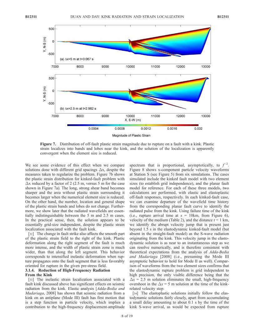
We see some evidence of this effect when we comparesolutions done with different grid spacings Dx, despite themeasures taken to regularize the problem. Figure 7b showsthe plastic strain distribution for kinked-fault problem withDx reduced by a factor of 2 (2.5 m, versus 5 m for the caseshown in Figure 7a). The long, strong shear band becomessharper and the area without plastic strain surrounding itbecomes larger when the numerical element size is reduced.On the other hand, the number, location and general shapeof the plastic strain bands and lobes do not change. Further-more, we show later that the radiated wavefields are essen-tially indistinguishable between the 5 m and 2.5 m cases.In the practical sense, then, the solution appears to beessentially grid-size independent, despite the plastic strainlocalization associated with the fault kink.[32] The change in fault strike also affects the smooth part

of the plastic strain field to the right of the kink. Plasticdeformation along the right segment of the fault is muchmore intense, and the width of plastic strain zone is muchwider, than that along the left segment. This behaviorcorresponds to intensified inelastic deformation when rup-ture propagates onto the fault segment that is less favorablyoriented for rupture in the given pre-stress field.3.1.4. Reduction of High-Frequency RadiationFrom the Kink[33] The inelastic strain localization associated with a

fault kink discussed above has significant effects on seismicradiation from the kink. Elastic analysis [Adda-Bedia andMadariaga, 2008] has shown that seismic radiation from akink on an antiplane (Mode III) fault has first motion thatis a step function in particle velocity, which implies acontribution to the high-frequency displacement-amplitude

spectrum that is proportional, asymptotically, to f�2.Figure 8 shows x-component particle velocity waveformsat Station S (see Figure 5) from six simulations. The casessimulated include the kinked fault model with two elementsizes (to establish grid independence), and the planar faultmodel for reference. For each of these three models, twocalculations are performed, with elastic and elastoplasticoff-fault responses, respectively. In each kinked-fault case,we can examine departure of the wavefield time historyfrom the corresponding planar fault curve to identify theradiated pulse from the kink. Using failure time of the kink(i.e., rupture arrival time at x = 10km, from Figure 6),velocity of the medium (Table 2), and the distance r = 1 km,we identify the abrupt velocity jump that is present justbeyond 1.5 s in the elastodynamic kinked-fault model (butabsent in the straight-fault model) as the S-wave radiationoriginating from the kink. This velocity jump in the elasto-dynamic solution is as near to an instantaneous step as wecan resolve numerically, and is therefore consistent withtheoretical expectations from the analysis of Adda-Bediaand Madariaga [2008] (i.e., presuming the Mode IIIasymptotic behavior to hold for Mode II as well). Compar-ison of waveforms from the two element sizes confirms thatthe elastodynamic rupture problem is grid independent tohigh precision, the only visible difference being that theDx = 2.5 m solution eliminates the small, high-frequencyovershoot in the Dx = 5 m solution at the time of the kink-related velocity step.[34] The elastoplastic solutions initially follow the elas-

todynamic solutions fairly closely, apart from accumulatinga small delay amounting to about 0.1 s by the time of thekink S-wave arrival, as would be expected from rupture

Figure 7. Distribution of off-fault plastic strain magnitude due to rupture on a fault with a kink. Plasticstrain localizes into bands and lobes near the kink, and the solution of the localization is apparentlyconvergent when the element size is reduced.


8 of 19

B12311

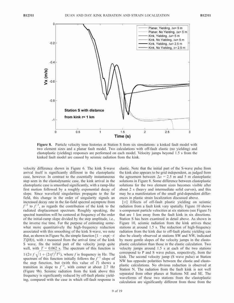
velocity difference shown in Figure 6. The kink S-wavearrival itself is significantly different in the elastoplasticcase, however. In contrast to the essentially instantaneousstep seen in the elastodynamic case, the kink arrival in theelastoplastic case is smoothed significantly, with a ramp-likefirst motion followed by a roughly exponential decay ofslope. Since wavefield singularities propagate to the farfield, this change in the order of singularity signals anincreased decay rate in the far-field spectral asymptote fromf�2 to f�3, as regards the contribution of the kink to theradiated displacement spectrum. Roughly speaking, thespectral transition will be centered at frequency of the orderof the initial-ramp slope divided by the step amplitude, i.e.,the inverse rise time. For the purpose of estimating some-what more quantitatively the high-frequency reductionassociated with this smoothing of the kink S-wave, we notethat, as shown in Figure 9a, the simple function [1� exp(�t/T)]H(t), with t measured from the arrival time of the kinkS wave, fits the initial part of the velocity jump quitewell, with T = 0.062 s. The spectrum of this function is

1/(2p f

ffiffiffiffiffiffiffiffiffiffiffiffiffiffiffiffiffiffiffiffiffiffiffiffiffiffiffi1þ 2pfð Þ2T2

q), where f is frequency in Hz. The

spectrum of this function initially follows the f�1 slope ofthe step function, but (with this value of T) shows atransition in slope to f�2, with corner at about 2.7 Hz(Figure 9b). Seismic radiation from the kink above thisfrequency is significantly reduced by off-fault plastic yield-ing, compared with the case in which off-fault response is

elastic. Note that the initial part of the S-wave pulse fromthe kink also appears to be grid independent, as judged fromthe agreement between Dx = 2.5 m and 5 m elastoplasticsolutions in Figure 8. Some difference between elastoplasticsolutions for the two element sizes becomes visible afterabout 2 s (heavy and intermediate solid curves), and thismay be a manifestation of the small grid-dependent differ-ences in plastic strain localization discussed above.[35] Effects of off-fault plastic yielding on seismic

radiation from a fault kink vary spatially. Figure 10 showsx-component particle velocities at six stations (see Figure 5)that are 1 km away from the fault kink in six directions.Station S has been examined in detail above. As shown inFigure 10, seismic radiation from the kink arrives thesestations at around 1.5 s. The reduction of high-frequencyradiation from the kink due to off-fault plastic yielding canalso be clearly observed at stations SW and NW, indicatedby more gentle slopes of the velocity jumps in the elasto-plastic calculation than those in the elastic calculation. Twovelocity jumps around 1.5 s at each of the two stationscorrespond to P and S wave pulses, respectively, from thekink. The second velocity jump (S wave pulse) at StationNW has opposite polarities between the elastic and elasto-plastic calculations. No obvious reduction is observed atStation N. The radiation from the fault kink is not wellseparated from other phases at Stations NE and SE. Thewaveforms of these two stations from the elastoplasticcalculation are significantly different from those from the

Figure 8. Particle velocity time histories at Station S from six simulations: a kinked fault model withtwo element sizes and a planar fault model. Two calculations with off-fault elastic (no yielding) andelastoplastic (yielding) responses are performed on each model. Velocity jumps beyond 1.5 s from thekinked fault model are caused by seismic radiation from the kink.


9 of 19

B12311

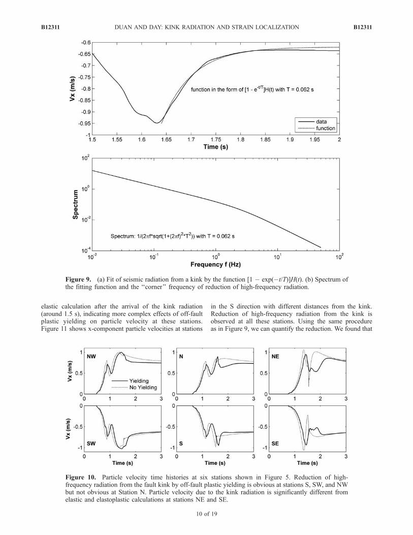
elastic calculation after the arrival of the kink radiation(around 1.5 s), indicating more complex effects of off-faultplastic yielding on particle velocity at these stations.Figure 11 shows x-component particle velocities at stations

in the S direction with different distances from the kink.Reduction of high-frequency radiation from the kink isobserved at all these stations. Using the same procedureas in Figure 9, we can quantify the reduction. We found that

Figure 9. (a) Fit of seismic radiation from a kink by the function [1 � exp(�t/T)]H(t). (b) Spectrum ofthe fitting function and the ‘‘corner’’ frequency of reduction of high-frequency radiation.

Figure 10. Particle velocity time histories at six stations shown in Figure 5. Reduction of high-frequency radiation from the fault kink by off-fault plastic yielding is obvious at stations S, SW, and NWbut not obvious at Station N. Particle velocity due to the kink radiation is significantly different fromelastic and elastoplastic calculations at stations NE and SE.


10 of 19

B12311

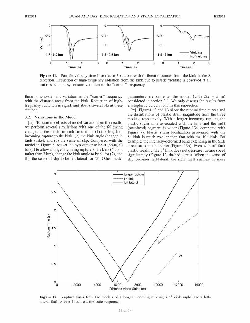
there is no systematic variation in the ‘‘corner’’ frequencywith the distance away from the kink. Reduction of high-frequency radiation is significant above several Hz at thesestations.

3.2. Variations in the Model

[36] To examine effects of model variations on the results,we perform several simulations with one of the followingchanges to the model in each simulation: (1) the length ofincoming rupture to the kink; (2) the kink angle (change infault strike); and (3) the sense of slip. Compared with themodel in Figure 5, we set the hypocenter to be at (5500, 0)for (1) to allow a longer incoming rupture to the kink (4.5 kmrather than 3 km), change the kink angle to be 5� for (2), andflip the sense of slip to be left-lateral for (3). Other model

parameters are same as the model (with Dx = 5 m)considered in section 3.1. We only discuss the results fromelastoplastic calculations in this subsection.[37] Figures 12 and 13 show the rupture time curves and

the distributions of plastic strain magnitude from the threemodels, respectively. With a longer incoming rupture, theplastic strain zone associated with the kink and the right(post-bend) segment is wider (Figure 13a, compared withFigure 7). Plastic strain localization associated with the5� kink is much weaker than that with the 10� kink. Forexample, the intensely-deformed band extending in the SEEdirection is much shorter (Figure 13b). Even with off-faultplastic yielding, the 5� kink does not decrease rupture speedsignificantly (Figure 12, dashed curve). When the sense ofslip becomes left-lateral, the right fault segment is more

Figure 11. Particle velocity time histories at 3 stations with different distances from the kink in the Sdirection. Reduction of high-frequency radiation from the kink due to plastic yielding is observed at allstations without systematic variation in the ‘‘corner’’ frequency.

Figure 12. Rupture times from the models of a longer incoming rupture, a 5� kink angle, and a left-lateral fault with off-fault elastoplastic response.


11 of 19

B12311

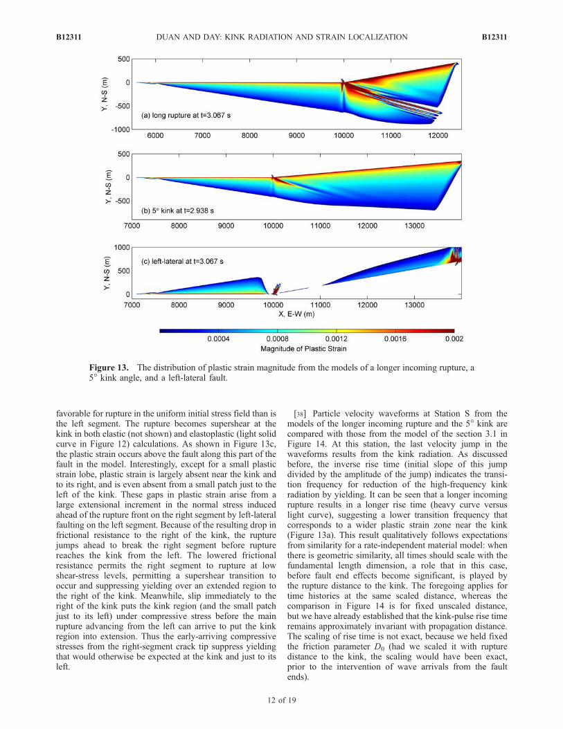
favorable for rupture in the uniform initial stress field than isthe left segment. The rupture becomes supershear at thekink in both elastic (not shown) and elastoplastic (light solidcurve in Figure 12) calculations. As shown in Figure 13c,the plastic strain occurs above the fault along this part of thefault in the model. Interestingly, except for a small plasticstrain lobe, plastic strain is largely absent near the kink andto its right, and is even absent from a small patch just to theleft of the kink. These gaps in plastic strain arise from alarge extensional increment in the normal stress inducedahead of the rupture front on the right segment by left-lateralfaulting on the left segment. Because of the resulting drop infrictional resistance to the right of the kink, the rupturejumps ahead to break the right segment before rupturereaches the kink from the left. The lowered frictionalresistance permits the right segment to rupture at lowshear-stress levels, permitting a supershear transition tooccur and suppressing yielding over an extended region tothe right of the kink. Meanwhile, slip immediately to theright of the kink puts the kink region (and the small patchjust to its left) under compressive stress before the mainrupture advancing from the left can arrive to put the kinkregion into extension. Thus the early-arriving compressivestresses from the right-segment crack tip suppress yieldingthat would otherwise be expected at the kink and just to itsleft.

[38] Particle velocity waveforms at Station S from themodels of the longer incoming rupture and the 5� kink arecompared with those from the model of the section 3.1 inFigure 14. At this station, the last velocity jump in thewaveforms results from the kink radiation. As discussedbefore, the inverse rise time (initial slope of this jumpdivided by the amplitude of the jump) indicates the transi-tion frequency for reduction of the high-frequency kinkradiation by yielding. It can be seen that a longer incomingrupture results in a longer rise time (heavy curve versuslight curve), suggesting a lower transition frequency thatcorresponds to a wider plastic strain zone near the kink(Figure 13a). This result qualitatively follows expectationsfrom similarity for a rate-independent material model: whenthere is geometric similarity, all times should scale with thefundamental length dimension, a role that in this case,before fault end effects become significant, is played bythe rupture distance to the kink. The foregoing applies fortime histories at the same scaled distance, whereas thecomparison in Figure 14 is for fixed unscaled distance,but we have already established that the kink-pulse rise timeremains approximately invariant with propagation distance.The scaling of rise time is not exact, because we held fixedthe friction parameter D0 (had we scaled it with rupturedistance to the kink, the scaling would have been exact,prior to the intervention of wave arrivals from the faultends).

Figure 13. The distribution of plastic strain magnitude from the models of a longer incoming rupture, a5� kink angle, and a left-lateral fault.


12 of 19

B12311

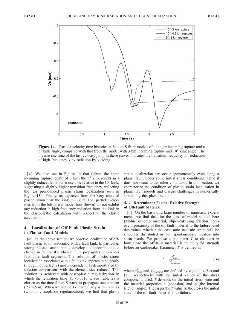
[39] We also see in Figure 14 that (given the sameincoming rupture length of 3 km) the 5� kink results in aslightly reduced kink-pulse rise time relative to the 10� kink,suggesting a slightly higher transition frequency, reflectingthe less pronounced plastic strain localization seen inFigure 13b. Finally, as expected from the very minimalplastic strain near the kink in Figure 13c, particle veloc-ities from the left-lateral model (not shown) do not exhibitany reduction in high-frequency radiation from the kink inthe elastoplastic calculation with respect to the elasticcalculation.

4. Localization of Off-Fault Plastic Strainin Planar Fault Models

[40] In the above section, we observe localization of off-fault plastic strain associated with a fault kink. In particular,strong plastic strain bands develop to accommodate achange in fault strike when rupture propagates onto a lessfavorable fault segment. The solution of plastic strainlocalization associated with a fault kink appears to be nearly(though not perfectly) grid independent, as demonstrated bysolution comparisons with the element size reduced. Thissolution is achieved with viscoplastic regularization inwhich the relaxation time Tv (0.0017 s, see Table 2) ischosen as the time for an S wave to propagate one element(Dx = 5 m). When we reduce Tv, particularly with Tv = 0 s(without viscoplastic regularization), we find that plastic

strain localization can occur spontaneously even along aplanar fault, under some initial stress conditions, while itdoes not occur under other conditions. In this section, wecharacterize the condition of plastic strain localization inplanar fault models and discuss challenges in numericallysimulating this phenomenon.

4.1. Determinant Factor: Relative Strengthof Off-Fault Material

[41] On the basis of a large number of numerical experi-ments, we find that, for the class of model studied here(Mohr-Coulomb material, slip-weakening friction), pre-event proximity of the off-fault material to the failure leveldetermines whether the coseismic inelastic strain will besmoothly distributed or will spontaneously localize intoshear bands. We propose a parameter T to characterizehow close the off-fault material is to the yield strengthbefore an earthquake. Parameter T is defined as

T ¼ t0max

t0coulomb; ð14Þ

where tmax0 and tcoulomb

0 are defined by equations (8b) and(11), respectively, with the initial values of the stresscomponents used. T depends on the initial stress state andthe material properties c (cohesion) and f (the internalfriction angle). The larger the T value is, the closer the initialstate of the off-fault material is to failure.

Figure 14. Particle velocity time histories at Station S from models of a longer incoming rupture and a5� kink angle, compared with that from the model with 3 km incoming rupture and 10� kink angle. Theinverse rise time of the last velocity jump in these curves indicates the transition frequency for reductionof high-frequency kink radiation by yielding.


13 of 19

B12311

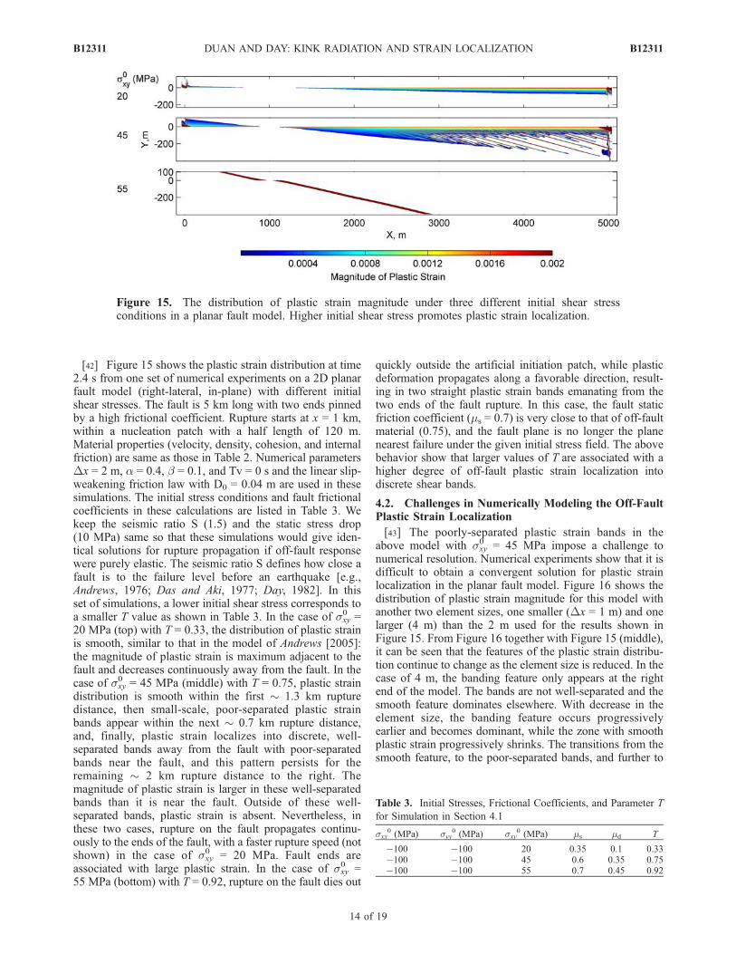
[42] Figure 15 shows the plastic strain distribution at time2.4 s from one set of numerical experiments on a 2D planarfault model (right-lateral, in-plane) with different initialshear stresses. The fault is 5 km long with two ends pinnedby a high frictional coefficient. Rupture starts at x = 1 km,within a nucleation patch with a half length of 120 m.Material properties (velocity, density, cohesion, and internalfriction) are same as those in Table 2. Numerical parametersDx = 2 m, a = 0.4, b = 0.1, and Tv = 0 s and the linear slip-weakening friction law with D0 = 0.04 m are used in thesesimulations. The initial stress conditions and fault frictionalcoefficients in these calculations are listed in Table 3. Wekeep the seismic ratio S (1.5) and the static stress drop(10 MPa) same so that these simulations would give iden-tical solutions for rupture propagation if off-fault responsewere purely elastic. The seismic ratio S defines how close afault is to the failure level before an earthquake [e.g.,Andrews, 1976; Das and Aki, 1977; Day, 1982]. In thisset of simulations, a lower initial shear stress corresponds toa smaller T value as shown in Table 3. In the case of sxy

0 =20 MPa (top) with T = 0.33, the distribution of plastic strainis smooth, similar to that in the model of Andrews [2005]:the magnitude of plastic strain is maximum adjacent to thefault and decreases continuously away from the fault. In thecase of sxy

0 = 45 MPa (middle) with T = 0.75, plastic straindistribution is smooth within the first 1.3 km rupturedistance, then small-scale, poor-separated plastic strainbands appear within the next 0.7 km rupture distance,and, finally, plastic strain localizes into discrete, well-separated bands away from the fault with poor-separatedbands near the fault, and this pattern persists for theremaining 2 km rupture distance to the right. Themagnitude of plastic strain is larger in these well-separatedbands than it is near the fault. Outside of these well-separated bands, plastic strain is absent. Nevertheless, inthese two cases, rupture on the fault propagates continu-ously to the ends of the fault, with a faster rupture speed (notshown) in the case of sxy

0 = 20 MPa. Fault ends areassociated with large plastic strain. In the case of sxy

0 =55 MPa (bottom) with T = 0.92, rupture on the fault dies out

quickly outside the artificial initiation patch, while plasticdeformation propagates along a favorable direction, result-ing in two straight plastic strain bands emanating from thetwo ends of the fault rupture. In this case, the fault staticfriction coefficient (ms = 0.7) is very close to that of off-faultmaterial (0.75), and the fault plane is no longer the planenearest failure under the given initial stress field. The abovebehavior show that larger values of T are associated with ahigher degree of off-fault plastic strain localization intodiscrete shear bands.

4.2. Challenges in Numerically Modeling the Off-FaultPlastic Strain Localization

[43] The poorly-separated plastic strain bands in theabove model with sxy

0 = 45 MPa impose a challenge tonumerical resolution. Numerical experiments show that it isdifficult to obtain a convergent solution for plastic strainlocalization in the planar fault model. Figure 16 shows thedistribution of plastic strain magnitude for this model withanother two element sizes, one smaller (Dx = 1 m) and onelarger (4 m) than the 2 m used for the results shown inFigure 15. From Figure 16 together with Figure 15 (middle),it can be seen that the features of the plastic strain distribu-tion continue to change as the element size is reduced. In thecase of 4 m, the banding feature only appears at the rightend of the model. The bands are not well-separated and thesmooth feature dominates elsewhere. With decrease in theelement size, the banding feature occurs progressivelyearlier and becomes dominant, while the zone with smoothplastic strain progressively shrinks. The transitions from thesmooth feature, to the poor-separated bands, and further to

Figure 15. The distribution of plastic strain magnitude under three different initial shear stressconditions in a planar fault model. Higher initial shear stress promotes plastic strain localization.

Table 3. Initial Stresses, Frictional Coefficients, and Parameter T

for Simulation in Section 4.1

sxx0 (MPa) syy

0 (MPa) sxy0 (MPa) ms md T

�100 �100 20 0.35 0.1 0.33�100 �100 45 0.6 0.35 0.75�100 �100 55 0.7 0.45 0.92


14 of 19

B12311

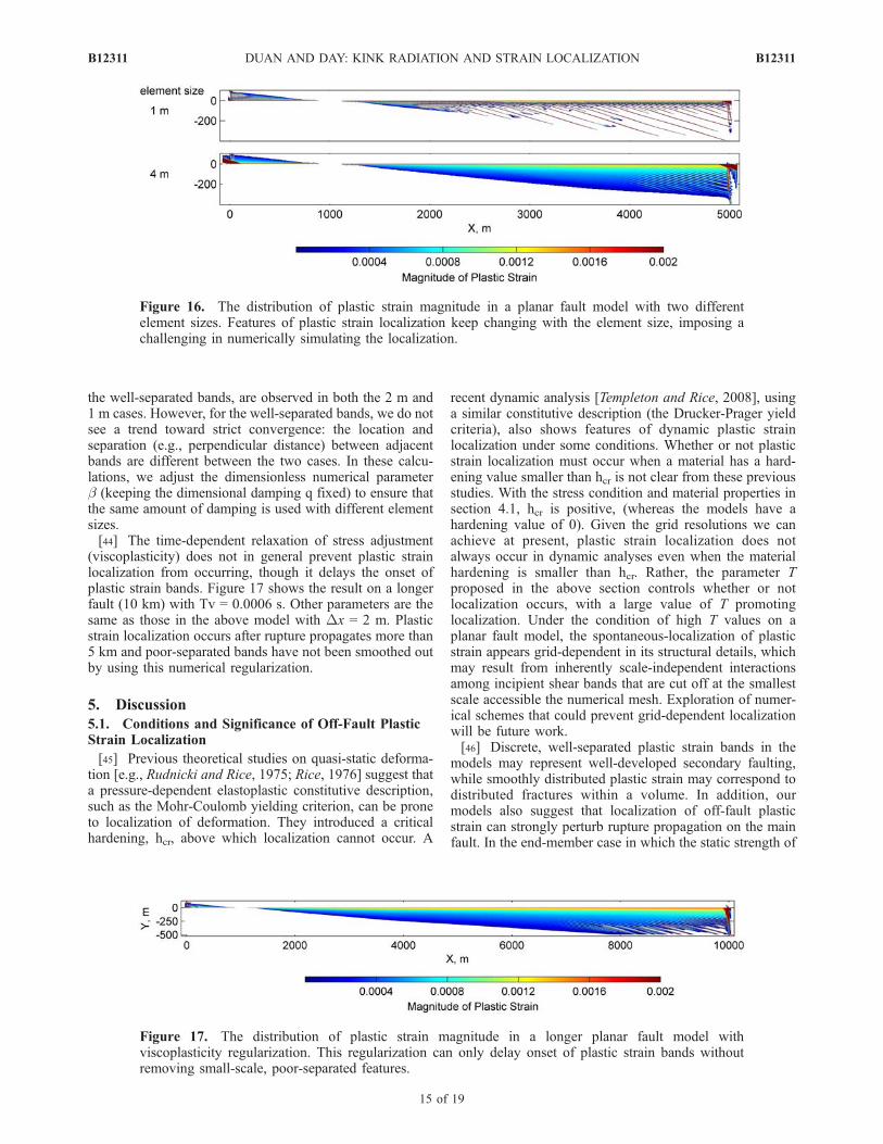
the well-separated bands, are observed in both the 2 m and1 m cases. However, for the well-separated bands, we do notsee a trend toward strict convergence: the location andseparation (e.g., perpendicular distance) between adjacentbands are different between the two cases. In these calcu-lations, we adjust the dimensionless numerical parameterb (keeping the dimensional damping q fixed) to ensure thatthe same amount of damping is used with different elementsizes.[44] The time-dependent relaxation of stress adjustment

(viscoplasticity) does not in general prevent plastic strainlocalization from occurring, though it delays the onset ofplastic strain bands. Figure 17 shows the result on a longerfault (10 km) with Tv = 0.0006 s. Other parameters are thesame as those in the above model with Dx = 2 m. Plasticstrain localization occurs after rupture propagates more than5 km and poor-separated bands have not been smoothed outby using this numerical regularization.

5. Discussion

5.1. Conditions and Significance of Off-Fault PlasticStrain Localization

[45] Previous theoretical studies on quasi-static deforma-tion [e.g., Rudnicki and Rice, 1975; Rice, 1976] suggest thata pressure-dependent elastoplastic constitutive description,such as the Mohr-Coulomb yielding criterion, can be proneto localization of deformation. They introduced a criticalhardening, hcr, above which localization cannot occur. A

recent dynamic analysis [Templeton and Rice, 2008], usinga similar constitutive description (the Drucker-Prager yieldcriteria), also shows features of dynamic plastic strainlocalization under some conditions. Whether or not plasticstrain localization must occur when a material has a hard-ening value smaller than hcr is not clear from these previousstudies. With the stress condition and material properties insection 4.1, hcr is positive, (whereas the models have ahardening value of 0). Given the grid resolutions we canachieve at present, plastic strain localization does notalways occur in dynamic analyses even when the materialhardening is smaller than hcr. Rather, the parameter Tproposed in the above section controls whether or notlocalization occurs, with a large value of T promotinglocalization. Under the condition of high T values on aplanar fault model, the spontaneous-localization of plasticstrain appears grid-dependent in its structural details, whichmay result from inherently scale-independent interactionsamong incipient shear bands that are cut off at the smallestscale accessible the numerical mesh. Exploration of numer-ical schemes that could prevent grid-dependent localizationwill be future work.[46] Discrete, well-separated plastic strain bands in the

models may represent well-developed secondary faulting,while smoothly distributed plastic strain may correspond todistributed fractures within a volume. In addition, ourmodels also suggest that localization of off-fault plasticstrain can strongly perturb rupture propagation on the mainfault. In the end-member case in which the static strength of

Figure 16. The distribution of plastic strain magnitude in a planar fault model with two differentelement sizes. Features of plastic strain localization keep changing with the element size, imposing achallenging in numerically simulating the localization.

Figure 17. The distribution of plastic strain magnitude in a longer planar fault model withviscoplasticity regularization. This regularization can only delay onset of plastic strain bands withoutremoving small-scale, poor-separated features.


15 of 19

B12311

the fault is close to the strength of the surrounding material,for example, off-fault strain bands develop while ruptureon the pre-existing fault dies out (e.g., in the model ofsxy0 = 55 MPa in section 4.1). Thus different damage

distributions in the field may give us some clues aboutrelative strength between a main fault and the surroundinghost rocks: if there is significant secondary faulting, it mayindicate the strength of the main fault is close to that of thehost rocks; more diffuse damage may be characteristic whenthe strength of the main fault is significantly lower than thatof the host rocks.

5.2. Effects of Off-Fault Plastic Yielding on ResidualStresses at a Fault Kink

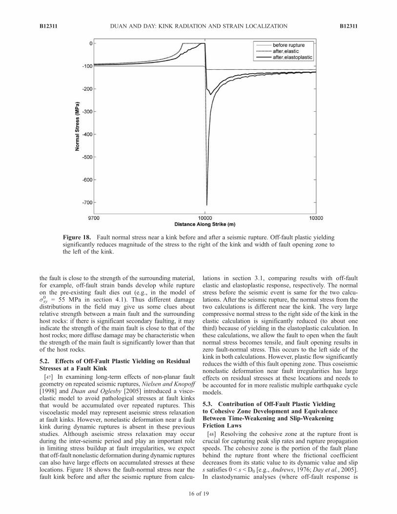
[47] In examining long-term effects of non-planar faultgeometry on repeated seismic ruptures, Nielsen and Knopoff[1998] and Duan and Oglesby [2005] introduced a visco-elastic model to avoid pathological stresses at fault kinksthat would be accumulated over repeated ruptures. Thisviscoelastic model may represent aseismic stress relaxationat fault kinks. However, nonelastic deformation near a faultkink during dynamic ruptures is absent in these previousstudies. Although aseismic stress relaxation may occurduring the inter-seismic period and play an important rolein limiting stress buildup at fault irregularities, we expectthat off-fault nonelastic deformation during dynamic rupturescan also have large effects on accumulated stresses at theselocations. Figure 18 shows the fault-normal stress near thefault kink before and after the seismic rupture from calcu-

lations in section 3.1, comparing results with off-faultelastic and elastoplastic response, respectively. The normalstress before the seismic event is same for the two calcu-lations. After the seismic rupture, the normal stress from thetwo calculations is different near the kink. The very largecompressive normal stress to the right side of the kink in theelastic calculation is significantly reduced (to about onethird) because of yielding in the elastoplastic calculation. Inthese calculations, we allow the fault to open when the faultnormal stress becomes tensile, and fault opening results inzero fault-normal stress. This occurs to the left side of thekink in both calculations. However, plastic flow significantlyreduces the width of this fault opening zone. Thus coseismicnonelastic deformation near fault irregularities has largeeffects on residual stresses at these locations and needs tobe accounted for in more realistic multiple earthquake cyclemodels.

5.3. Contribution of Off-Fault Plastic Yieldingto Cohesive Zone Development and EquivalenceBetween Time-Weakening and Slip-WeakeningFriction Laws

[48] Resolving the cohesive zone at the rupture front iscrucial for capturing peak slip rates and rupture propagationspeeds. The cohesive zone is the portion of the fault planebehind the rupture front where the frictional coefficientdecreases from its static value to its dynamic value and slips satisfies 0 < s < D0 [e.g., Andrews, 1976; Day et al., 2005].In elastodynamic analyses (where off-fault response is

Figure 18. Fault normal stress near a kink before and after a seismic rupture. Off-fault plastic yieldingsignificantly reduces magnitude of the stress to the right of the kink and width of fault opening zone tothe left of the kink.


16 of 19

B12311

assumed to be purely elastic), a linear slip-weakeningfriction law with a constant critical slip distance D0 resultsin shrinking of the cohesive zone width with increasingrupture velocity vr, the width approaching zero as terminalvelocity (the Rayleigh velocity in the plane strain case) isapproached. Rupture velocity in turn grows with rupturepropagation distance (assuming conditions of uniform stressdrop and 2D geometry), so the cohesive-zone width con-tracts with propagation distance in the elastodynamic case.A linear time-weakening friction law can avoid this narrow-ing of the cohesive zone with propagation distance, andresults in an effective D0 that is proportional to the squareroot of rupture propagation distance [Andrews, 2004; Day etal., 2005].[49] With off-fault plastic yielding, however, the cohesive

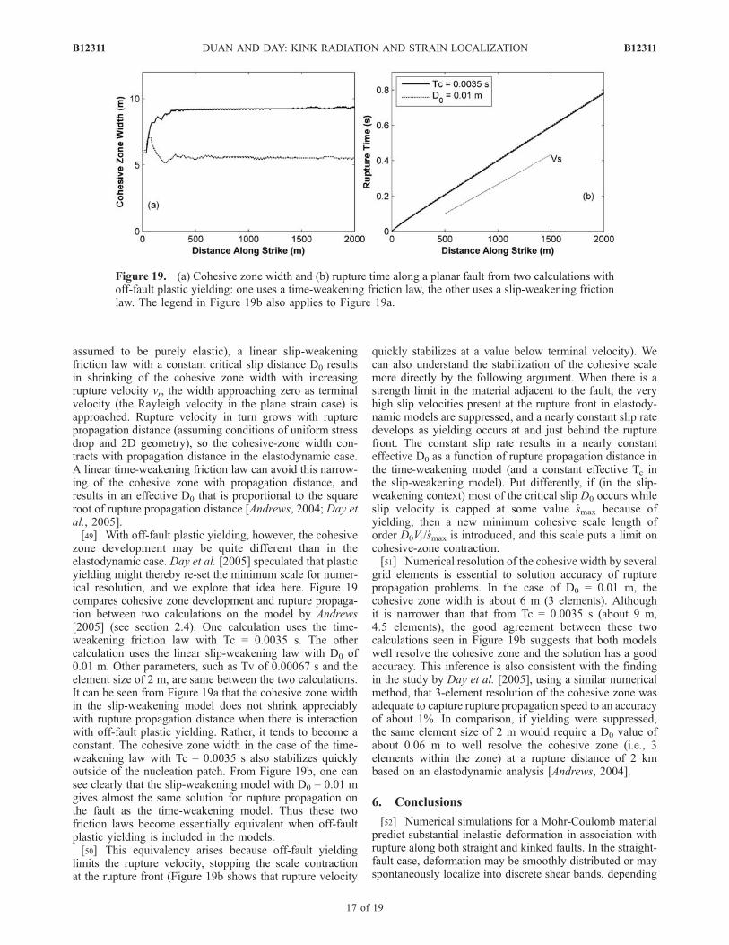
zone development may be quite different than in theelastodynamic case. Day et al. [2005] speculated that plasticyielding might thereby re-set the minimum scale for numer-ical resolution, and we explore that idea here. Figure 19compares cohesive zone development and rupture propaga-tion between two calculations on the model by Andrews[2005] (see section 2.4). One calculation uses the time-weakening friction law with Tc = 0.0035 s. The othercalculation uses the linear slip-weakening law with D0 of0.01 m. Other parameters, such as Tv of 0.00067 s and theelement size of 2 m, are same between the two calculations.It can be seen from Figure 19a that the cohesive zone widthin the slip-weakening model does not shrink appreciablywith rupture propagation distance when there is interactionwith off-fault plastic yielding. Rather, it tends to become aconstant. The cohesive zone width in the case of the time-weakening law with Tc = 0.0035 s also stabilizes quicklyoutside of the nucleation patch. From Figure 19b, one cansee clearly that the slip-weakening model with D0 = 0.01 mgives almost the same solution for rupture propagation onthe fault as the time-weakening model. Thus these twofriction laws become essentially equivalent when off-faultplastic yielding is included in the models.[50] This equivalency arises because off-fault yielding

limits the rupture velocity, stopping the scale contractionat the rupture front (Figure 19b shows that rupture velocity

quickly stabilizes at a value below terminal velocity). Wecan also understand the stabilization of the cohesive scalemore directly by the following argument. When there is astrength limit in the material adjacent to the fault, the veryhigh slip velocities present at the rupture front in elastody-namic models are suppressed, and a nearly constant slip ratedevelops as yielding occurs at and just behind the rupturefront. The constant slip rate results in a nearly constanteffective D0 as a function of rupture propagation distance inthe time-weakening model (and a constant effective Tc inthe slip-weakening model). Put differently, if (in the slip-weakening context) most of the critical slip D0 occurs whileslip velocity is capped at some value _smax because ofyielding, then a new minimum cohesive scale length oforder D0Vr/_smax is introduced, and this scale puts a limit oncohesive-zone contraction.[51] Numerical resolution of the cohesive width by several

grid elements is essential to solution accuracy of rupturepropagation problems. In the case of D0 = 0.01 m, thecohesive zone width is about 6 m (3 elements). Althoughit is narrower than that from Tc = 0.0035 s (about 9 m,4.5 elements), the good agreement between these twocalculations seen in Figure 19b suggests that both modelswell resolve the cohesive zone and the solution has a goodaccuracy. This inference is also consistent with the findingin the study by Day et al. [2005], using a similar numericalmethod, that 3-element resolution of the cohesive zone wasadequate to capture rupture propagation speed to an accuracyof about 1%. In comparison, if yielding were suppressed,the same element size of 2 m would require a D0 value ofabout 0.06 m to well resolve the cohesive zone (i.e., 3elements within the zone) at a rupture distance of 2 kmbased on an elastodynamic analysis [Andrews, 2004].

6. Conclusions

[52] Numerical simulations for a Mohr-Coulomb materialpredict substantial inelastic deformation in association withrupture along both straight and kinked faults. In the straight-fault case, deformation may be smoothly distributed or mayspontaneously localize into discrete shear bands, depending

Figure 19. (a) Cohesive zone width and (b) rupture time along a planar fault from two calculations withoff-fault plastic yielding: one uses a time-weakening friction law, the other uses a slip-weakening frictionlaw. The legend in Figure 19b also applies to Figure 19a.


17 of 19

B12311

upon the initial stress state and the material strengthparameters (i.e., cohesion and internal friction). For uniforminitial stress, the determinative parameter controlling spon-taneous localization is the ratio tmax/tcoulomb (defined byequations (8b) and (11)). If these distinct damage modes(smoothly distributed versus localized) arising in idealizedmodels have approximate counterparts in real faulting, thenfield patterns of damage and secondary faulting may pro-vide information about relative strength between faultsurface and host rock, with, e.g., a more localized damagemode being inductive of bulk and frictional strength that arerelatively close in value.[53] In the case of a kinked-fault, extensive inelastic

deformation concentrates near a restraining bend, principallyon the side of the fault associated with rupture-frontextensional strains, the deformation taking the form of afew distinct lobes and shear bands. The spatial extent andintensity of the deformation both increase with increasingrestraining-bend angle, and become relatively much smallerin the case of a releasing-bend orientation. For someazimuths, the inelastic strain reduces the high-frequencyseismic radiation originating from the kink, with the far-field spectrum of this phase diminishing by an extra factorof f�1 (relative to the corresponding perfectly elastic model),above a frequency of several Hz. The coseismic inelasticstrain also greatly reduces the residual stress concentrationsleft behind after rupture through a fault bend (e.g., residualnormal stress reduction of a factor of 3 in a typical 10�restraining bend case), with potentially significant con-sequences for models of fault-system evolution throughmultiple-earthquake cycles.[54] Rupture simulations for the Mohr-Coulomb material

model raise some computational issues not present incorresponding perfectly elastic problems. Our comparisonwith published results by Andrews [2005] suggests thatnumerical solutions for those rupture models with smoothstrain distributions can be reproduced to high precisionwhen done with different numerical methods and different(but sufficiently refined) grids. When localized shear bandsare induced at an isolated, discrete concentrator like a faultkink, the essential features of the solution appear to be gridindependent, but some grid dependence persists in thedetails of the final strain distribution. Finally, in the casewhere multiple shear bands develop spontaneously, thebands appear to interact strongly at the smallest spatialscales accessible to the grid, and we therefore do not obtainstrict numerical convergence as the grid is refined. On theother hand, plastic yielding suppresses the scale contractionof the fault cohesive zone that otherwise occurs in perfectlyelastic rupture propagation models, thereby improving theprospects for numerical resolution of the short-scale lengthsinduced by frictional breakdown.

[55] Acknowledgments. We are grateful to D. J. Andrews for pro-viding data and image files for facilitating the code comparison. Careful anddetailed reviews by R. Madariaga, E. Templeton, and the associate editorimproved our presentation. This research was supported by the SouthernCalifornia Earthquake Center through a grant from the U.S. Department ofEnergy/Pacific Gas and Electric Extreme Ground Motions project, as wellas by USGS grant 08HQGR0048 and NSF grant ATM-0325033. The SCECcontribution number for this paper is 1198.

ReferencesAdda-Bedia, M., and R. Madariaga (2008), Seismic radiation from a kinkon an antiplane fault, Bull. Seismol. Soc. Am., 98, 2291 – 2302,doi:10.1785/0120080003.

Andrews, D. J. (1976), Rupture velocity of plane strain shear cracks,J. Geophys. Res., 81(32), 5679–5687.

Andrews, D. J. (1999), Test of two methods for faulting in finite-differencecalculations, Bull. Seismol. Soc. Am., 89(4), 931–937.

Andrews, D. J. (2004), Rupture models with dynamically-determinedbreakdown displacement, Bull. Seismol. Soc. Am., 94, 769–775.

Andrews, D. J. (2005), Rupture dynamics with energy loss outside the slipzone, J. Geophys. Res., 110, B01307, doi:10.1029/2004JB003191.

Andrews, D. J., T. C. Hanks, and J. W. Whitney (2007), Physical limits onground motion at Yucca Mountain, Bull. Seismol. Soc. Am., 97, 1771–1792, doi:10.1785/0120070014.

Aochi, H., E. Fukuyama, and M. Matsu’ura (2000), Spontaneous rupturepropagation on a non-planar fault in 3-D elastic medium, Pure Appl.Geophys., 157, 2003–2037.

Ben-Zion, Y., and C. G. Sammis (2003), Characterization of fault zones,Pure Appl. Geophys., 160, 677–715.

Ben-Zion, Y., Z. Peng, D. Okaya, L. Seeber, L. G. Armbruster, N. Ozer, A. J.Michael, S. Baris, and M. Aktar (2003), A shallow fault zone structureilluminated by trapped waves in the Karadere-Duzce branch of the NorthAnatolian fault, western Turkey, Geophys. J. Int., 152, 699 – 717,doi:10.1046/j.1365-246X.2003.01870.x.

Bouchon, M., and D. Streiff (1997), Propagation of a shear crack on anonplanar fault: A method of calculation, Bull. Seismol. Soc. Am., 87,61–66.

Chester, F. M., and J. S. Chester (1998), Unltrcataclasite structure andfriction processes of the Punchbowl, San Andreas system, California,Tectonophysics, 295, 199–221.

Chester, F. M., J. S. Chester, D. L. Kirschner, S. E. Schulz, and J. P. Evans(2004), Structure of large-displacement strike-slip fault zones in the brittlecontinental crust, in Rheology and Deformation in the Lithosphere atContinental Margins, MARGINS Theor. and Exp. Earth Sci. Ser., vol. 1,edited by G. D. Karner et al., pp. 223–260, Columbia Univ. Press,New York.

Dalguer, L. A., and S. M. Day (2007), Staggered-grid split-node method forspontaneous rupture simulation, J. Geophys. Res., 112, B02302,doi:10.1029/2006JB004467.

Das, S., and K. Aki (1977), A numerical study of two-dimensional sponta-neous rupture propagation, Geophys. J. R. Astron. Soc., 50, 643–668.

Davis, R. O., and A. P. S. Selvadurai (2002), Plasticity and Geomechanics,Cambridge Univ. Press, Cambridge, New York.

Day, S. M. (1982), Three-dimensional simulation of spontaneous rupture:The effect of nonuniform prestress, Bull. Seismol. Soc. Am., 72, 1881–1902.

Day, S. M., L. A. Dalguer, N. Lapusta, and Y. Liu (2005), Comparison offinite difference and boundary integral solutions to three-dimensionalspontaneous rupture, J. Geophys. Res., 110, B12307, doi:10.1029/2005JB003813.

Duan, B., and D. D. Oglesby (2005), Multicycle dynamics of nonplanarstrike-slip faults, J. Geophys. Res., 110, B03304, doi:10.1029/2004JB003298.

Duan, B., and D. D. Oglesby (2006), Heterogeneous fault stresses fromprevious earthquakes and the effect on dynamics of parallel strike-slipfaults, J. Geophys. Res., 111, B05309, doi:10.1029/2005JB004138.

Duan, B., and D. D. Oglesby (2007), Nonuniform prestress from prior earth-quakes and the effect on dynamics of branched fault systems, J. Geophys.Res., 112, B05308, doi:10.1029/2006JB004443.

Ellsworth, W. L., and P. Malin (2006), A first observation of fault guidedPSV-waves at SAFOD and its implications for fault characteristics, EosTrans. AGU, 87(52), Fall Meet. Suppl., Abstract T23E-02.

Ely, G., S. M. Day, and J.-B. Minster (2008), A support-operator methodfor 3D rupture dynamics, Geophys. J. Int., in review.

Hughes, T. J. R. (2000), The Finite Element Method: Linear Static andDynamic Finite Element Analysis, Dover, Nineola, New York.

King, G., and J. Nabelek (1985), Role of fault bends in the initiation andtermination of earthquake rupture, Science, 228, 984–987.

Li, Y. G., K. Aki, D. Adams, A. Hasemi, and W. H. K. Lee (1994), Seismicguided waves trapped in the fault zone of the Landers, California, earth-quake of 1992, J. Geophys. Res., 99, 11,705–11,722.

Madariaga, R. (1977), High frequency radiation from crack (stress drop)models of earthquake faulting, Geophys. J. R. Astron. Soc., 51, 625–651.

Nielsen, S. B., and L. Knopoff (1998), The equivalent strength of geome-trical barriers to earthquakes, J. Geophys. Res., 103(B5), 9953–9965.

Poliakov, A. N. B., R. Dmowska, and J. R. Rice (2002), Dynamic shearrupture interactions with fault bends and off-axis secondary faulting,J. Geophys. Res., 107(B11), 2295, doi:10.1029/2001JB000572.


18 of 19

B12311

Rice, J. R. (1976), The localization of plastic deformation, in Theoreticaland Applied Mechanics, Proceedings of the 14th International Congresson Theoretical and Applied Mechanics, Delft, 1976, vol. 1, edited byW. T. Koiter, pp. 207–220, North-Holland, New York.

Rice, J. R., C. G. Sammis, and R. Parsons (2005), Off-fault secondaryfailure induced by a dynamic slip pulse, Bull. Seismol. Soc. Am., 95(1),109–134, doi:10.1785/0120030166.

Rudnicki, J. W., and J. R. Rice (1975), Conditions for the localization ofdeformation in pressure-sensitive dilatant materials, J. Mech. Phys. Solids,23, 371–394.

Scholz, C. H. (2002), The Mechanics of Earthquakes and Faulting, 2nd ed.,Cambridge Univ. Press, New York.

Tada, T., and T. Yamashita (1997), Non-hypersingular boundary integralequations for two-dimensional non-planar crack analysis, Geophys. J. Int.,130, 269–282.

Templeton, E. L., and J. R. Rice (2008), Off-fault plasticity and earthquakerupture dynamics. 1: Dry materials or neglect of fluid pressure changes,J. Geophys. Res., 113, B09306, doi:10.1029/2007JB005529.

��S. M. Day, Department of Geological Sciences, San Diego State

University, 5500 Campanile Dr., San Diego, CA 92182, USA.B. Duan, Department of Geology and Geophysics, Texas A&M

University, 3115 TAMU, College Station, TX 77843-3115, USA.([email protected])


19 of 19

B12311

Documents

Inelastic strain distribution and seismic radiation from ...people.tamu.edu/~bduan/Duan_2008JB005847.pdf · Inelastic strain distribution and seismic radiation from rupture of a fault