Geol. Soc. Malaysia, Bulletin 25, December 1989; pp. 53 - 63

Seismic. processing applications on a personal computer

Geophysical Service (Malaysia) Sdn. Bhd.

Lam Soon Industrial Building

63, Hillview Avenue,# 08-23

Singapore 2366

Abstract : This paper demonstrates the "state-of-the-art" processing that has been moved from a mainframe environment to the small office/desk-top machine. Although the data examples are combined to demonstrate a vertical seismic processing example, it will be stressed that this application is just an example of a particular grouping of seismic programmes from the software library.

As mainframe computers increase in capacity and speed, the personal computers are reducing in size, but not in power. The personal computer will be increasingly used in decision making based on small subsets of data whilst interacting with the mainframe as a workstation.

INTRODUCTION

Tasks such as project start-up, testing and modelling call for large numbers of jobs but relatively little computing power. If tests on small subsets of data are moved to a personal computer (PC workstation), turnaround time is reduced as time spent in job queues on the mainframe and waiting for hard-copy displays is saved. On a PC workstation the tests, selection of results based on them, and review of the data at various stages can be done in an efficient way.

Some of the larger tasks that can now be performed on a PC workstation include refraction modelling, vertical seismic profiling (VSP) and velocity modelling for CDP stacking. Before we look at VSP processing as an example of the use of PC workstations in seismic processing we will have a brief overview of the VSP method and its objectives.

THE VERTICAL SEISMIC PROFILING (VSP) METHOD

A vertical seismic profile is a small scale seismic survey recorded with the seismic source at or near the surface and a receiver down the borehole. The source may be at or close to the wellhead (zero-offset VSPS). This would create reflection points close to the borehole. If the source were offset from the wellhead(offset VSPS), or the well were deviated, reflection points at some distance from the borehole would be generated. Receivers are located at different depths down the borehole. More than one recording may be taken at each depth.

Presented at GSM Petroleum Geology Seminar 1988

54 GEOPHYSICAL SERVICE (M) SoN. BHD.

Objectives of the VSP method may be summarized as follows:-

1) Accurate depth to reflectors observed on surface seismic data,

2) Recognition of multiple reflections,

3) Measurement of accurate interval velocities,

4) Method for studying attenuation,

5) Measurement of shear wave velocities,

6) High resolution structural and stratigraphic delineation near the well,

7) Capability to "Look ahead of the bit".

VSP PROCESSING

A VSP is unique compared to conventional seismic recording in that both upgoing and downgoing wavefields are recorded. The downgoing wavefield consists of direct waves from the surface source and downgoing multiples. The upgoing wavefield comprises upgoing energy travelling back towards the surface as primary reflections and upgoing multiples. VSPS therefore contain information about the reflection and transmission properties of the earth.

To recover this information the data must be processed to separate the upgoing and downgoing wavefields and the results studied in relation to surface recorded data.

The PC workstation VSP processing system we are considering is a modular seismic data processing system which allows the user to process VSPS from field data through to a final product. The program modules are designed to work together through an MS-DOS batch processing file. This allows the user to run a pre-planned processing sequence which may last several hours, and execute different programs with little or no user interaction with the computer after starting the programs.

During screen displays there is also an interactive processing capability for edit, event picking, flattening and stack.

There are basically two paths in a VSP processing flowchart, one for zero­offset processing and a variation for offset processing. Once the field data has been reformated to PC format a fairly standard zero-offset processing sequence would consist of the following:-

1) Ordering and vertically stacking common depth traces,

2) Separating downgoing and upgoing energy,

3) Deconvolving the source signature,

4) Correcting for absorption and spreading loss, and

SEISMIC PROCESSING APPLICATIONS ON A PERSONAL CoMPUTER 55

5) Flattening on the upgoing energy and corridor stacking.

In offset VSP processing the first four steps are the same as for zero offset processing. Subsequently the data has to be mapped to true spatial position before it can be displayed as a small 2D seismic section in CDP-time space.

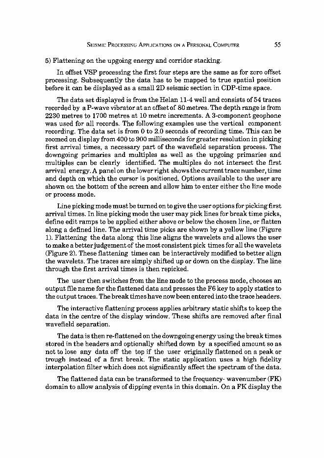
The data set displayed is from the Helan 11-4 well and consists of 54 traces recorded by a P-wave vibrator at an offset of 80 metres. The depth range is from 2230 metres to 1700 metres at 10 metre increments. A 3-component geophone was used for all records. The following examples use the vertical component recording. The data set is from 0 to 2.0 seconds of recording time. This can be zoomed on display from 400 to 900 milliseconds for greater resolution in picking first arrival times, a necessary part of the wavefield separation process. The downgoing primaries and multiples as well as the upgoing primaries and multiples can be clearly identified. The multiples do not intersect the first arrival energy. A panel on thelowerright showsthecurrenttracenumber, time and depth on which the cursor is positioned. Options available to the user are shown on the bottom of the screen and allow him to enter either the line mode or process mode.

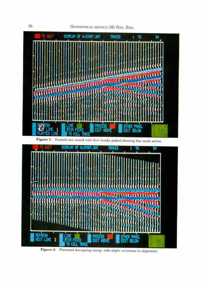
Line picking mode must be turned on to give the user options for picking first arrival times. In line picking mode the user may pick lines for break time picks, define edit ramps to be applied either above or below the chosen line, or flatten along a defined line. The arrival time picks are shown by a yellow line (Figure 1). Flattening the data along this line aligns the wavelets and allows the user to make a better judgement of the most consistent pick times for all the wavelets (Figure 2). These flattening times can be interactively modified to better align the wavelets. The traces are simply shifted up or down on the display. The line through the first arrival times is then repicked.

The user then switches from the line mode to the process mode, chooses an output file name for the flattened data and presses the F6 key to apply statics to the output traces. The break times have now been entered into the trace headers.

The interactive flattening process applies arbitrary static shifts to keep the data in the centre of the display window. These shifts are removed after final wavefield separation.

The data is then re-flattened on the downgoing energy using the break times stored in the headers and optionally shifted down by a specified amount so as not to lose any data off the top if the user originally flattened on a peak or trough instead of a first break. The static application uses a high fidelity interpolation filter which does not significantly affect the spectrum of the data.

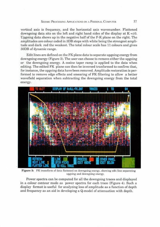
The flattened data can be transformed to the frequency- wavenumber (FK) domain to allow analysis of dipping events in this domain. On a FK display the

56 GEOPHYSICAL SERVICE (M) SDN. BHD.

Figure 1: Zoomed raw record with first breaks picked showing line mode active.

Figure 2: Flattened downgoing energy with slight variations in alignment.

SEI SM IC PROCESSING APPLICATIONS ON A P ERSONAL COMPUTER 57

vertical axis is frequency, and the horizontal axis wavenumber. Flattened downgoing data sits on the left and right hand sides of the display at K =±0. Upgoing data shows up in the negative half of the F-K plane on the right. The amplitudes are colour coded in 3DB steps with white being the strongest ampli­tude and dark red the weakest. The total colour scale has 11 colours and gives 30DB of dynamic range.

Edit lines are defined on the FK plane data to separate upgoing energy from downgoing energy (Figure 3). The user can choose to remove either the upgoing or the downgoing energy. A cosine taper ramp is applied to the data when editing. The edited FK plane can then be inversed tranformed to confirm that, for instance, the upgoing data have been removed. Amplitude restoration is per­formed to remove edge effects and smearing of FK filtering to allow a better wavefield separation when subtracting the downgoing energy from the total energy.

Figure 3: FK transform of data flattened on downgoing energy, showing edit line separating upgoing and downgoing energy.

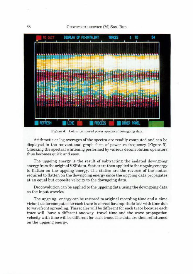
Power spectra can be computed for all the downgoing traces and displayed in a colour contour mode as power spectra for each trace (Figure 4). Such a display format is useful for analyzing loss of amplitude as a function of depth and frequency as an aid in developing a Q-model of attenuation with depth.

58 GEOPHYSICAL SERVICE (M) SDN. BHD.

Figure 4: Colour contoured power spectra of downgoing data.

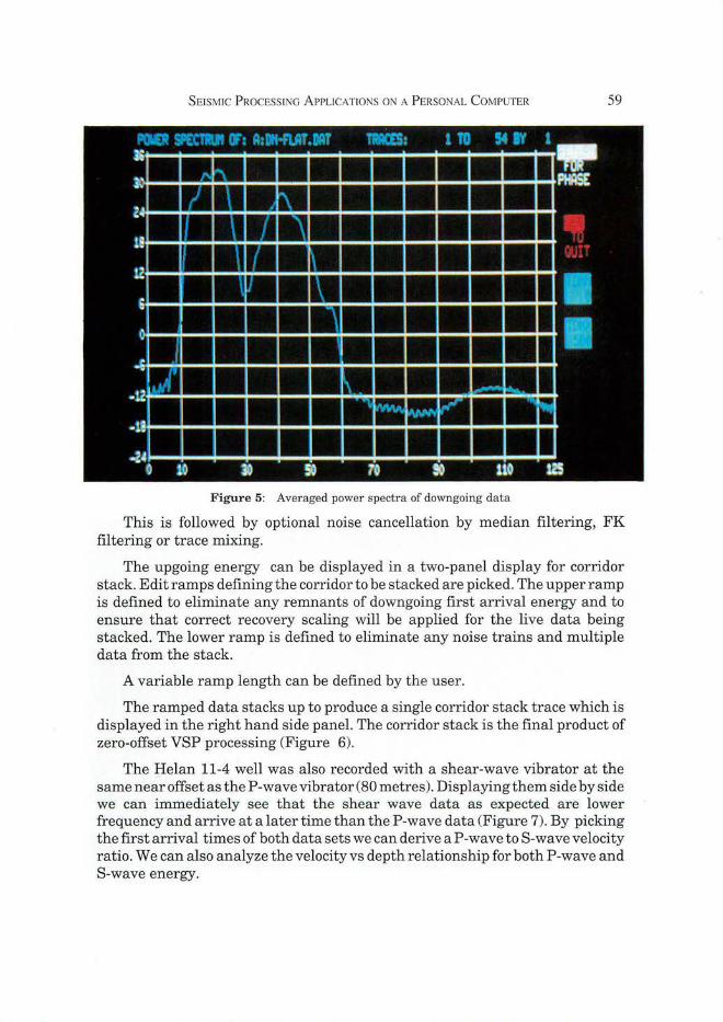
Arithmetic or log averages of the spectra are readily computed and can be displayed in the conventional graph form of power vs frequency (Figure 5). Checking the spectral whitening performed by various deconvolution operators thus becomes quick and easy.

The upgoing energy is the result of subtracting the isolated downgoing energy from the original VSP data. Statics are then applied to the up going energy to flatten on the upgoing energy. The statics are the reverse of the statics required to flatten on the downgoing energy since the upgoing data propagates at an equal but opposite velocity to the downgoing data.

Deconvolution can be applied to the upgoing data using the downgoing data as the input wavelet.

The upgoing energy can be restored to original recording time and a time viriant scaler computed for each trace to correct for amplitude loss with time due to wavefront spreading. This scaler will be different for each trace because each trace will have a different one-way travel time and the wave propagation velocity with time will be different for each trace. The data are then reflattened on the upgoing energy.

S EISMIC PROCESS ING APPLICATIONS ON A P ERSONAL C OM PUTER 59

Figure 5: Averaged power spectra of downgoing dat a

This is followed by optional noise cancellation by median filtering, FK filtering or trace mixing.

The upgoing energy can be displayed in a two-panel display for corridor stack. Edit ramps defining the corridor to be stacked are picked. The upper ramp is defined to eliminate any remnants of downgoing first arrival energy and to ensure that correct recovery scaling will be applied for the live data being stacked. The lower ramp is defined to eliminate any noise trains and multiple data from the stack.

A variable ramp length can be defined by the user.

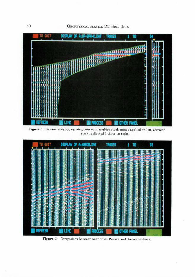
The ramped data stacks up to produce a single corridor stack trace which is displayed in the right hand side panel. The corridor stack is the final product of zero-offset VSP processing (Figure 6).

The Helan 11-4 well was also recorded with a shear-wave vibrator at the same near offset as the P-wave vibrator (80 metres). Displaying them side by side we can immediately see that the shear wave data as expected are lower frequency and arrive at a later time than the P-wave data (Figure 7). By picking the first arrival times of both data sets we can derive a P-wave to S-wave velocity ratio. We can also analyze the velocity vs depth relationship for both P-wave and S-wave energy.

60 GEOPHYSICAL SERVICE (M ) SnN. B HD.

Figure 6: 2-panel display, upgoing data with corridor stack ramps applied on left, corridor stack replicated 3 times on right.

Figure 7: Comparison between near offset P-wave and S-wave sections.

SEISMIC PROCESS ING APPLICATIONS ON A P ERSONAL COMPUTER 61

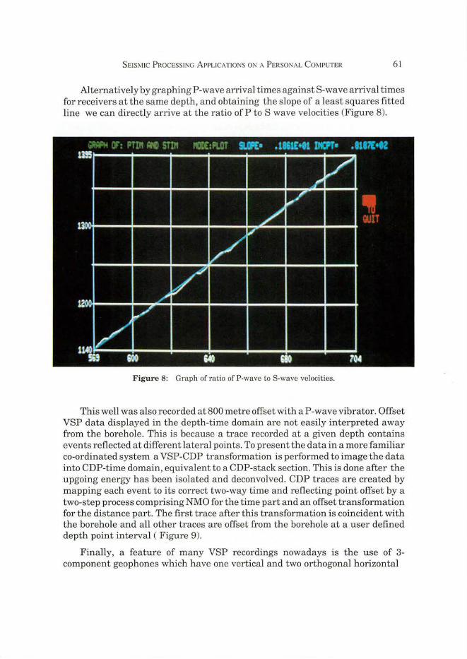
Alternatively by graphing P-wave arrival times against S-wave arrival times for receivers at the same depth, and obtaining the slope of a least squares fitted line we can directly arrive at the ratio of P to S wave velocities (Figure 8).

· · · SlOP£• .1861£+01 m:PT• .8197£•02 liS • ~ ...

•• ':~'~

1~

Ill· !:.11

IS-II"'

"'""" .... ,;l'ioll

/ llli :i'

l1tl 600 104

Figure 8: Graph of ratio of P-wave to S-wave velocities.

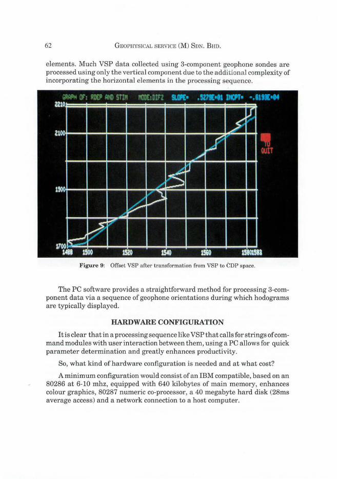
This well was also recorded at 800 metre offset with a P-wave vibrator. Offset VSP data displayed in the depth-time domain are not easily interpreted away from the borehole. This is because a trace recorded at a given depth contains events reflected at different lateral points. To present the data in a more familiar co-ordinated system a VSP-CDP transformation is performed to image the data into CDP-time domain, equivalent to a CDP-stack section. This is done after the upgoing energy has been isolated and deconvolved. CDP traces are created by mapping each event to its correct two-way time and reflecting point offset by a two-step process comprising NMO for the time part and an offset transformation for the distance part. The first trace after this transformation is coincident with the borehole and all other traces are offset from the borehole at a user defined depth point interval ( Figure 9).

Finally, a feature of many VSP recordings nowadays is the use of 3-component geophones which have one vertical and two orthogonal horizontal

62 GEOPHYSICAL SERVICE (M) SDN. B HD.

elements. Much VSP data collected using 3-component geophone sondes are processed using only the vertical component due to the additional complexity of incorporating the horizontal elements in the processing sequence.

Figure 9: Offset VSP after transformation from VSP to CDP space.

The PC software provides a straightforward method for processing 3-com­ponent data via a sequence of geophone orientations during which hodograms are typically displayed.

HARDWARE CONFIGURATION

It is clear that in a processing sequence like VSP that calls for strings of com­mand modules with user interaction between them, using a PC allows for quick parameter determination and greatly enhances productivity.

So, what kind of hardware configuration is needed and at what cost?

A minimum configuration would consist of an IBM compatible, based on an 80286 at 6-10 mhz, equipped with 640 kilobytes of main memory, enhances colour graphics, 80287 numeric co-processor, a 40 megabyte hard disk (28ms average access) and a network connection to a host computer.

SEISMIC PROCESSING APPLICATIONS ON A PERSONAL COMPUTER 63

A system consisting of an IBM-compatible 80386 at 16-25 mhz with 80387 numeric co-processor, 1 megabyte of main memory, VGA graphics and a larger hard disk in the 100 megabyte range would provide improved system perform­ance. A mouse, a laser printer capable of printing graphics and letter quality documents, and a digitizing tablet might be included. Such a system could cost less than $10,000 US dollars. .

Manuscipt received 2nd May 1989