Embed Size (px)
Citation preview
J. Inv. Ill-Posed Problems 18 (2011), 823–838DOI 10.1515/JIIP.2011.005 © de Gruyter 2011
Seismic impedance inversion using l1-normregularization and gradient descent methods
Yanfei Wang
Abstract. We consider numerical solution methods for seismic impedance inversion prob-lems in this paper. The inversion process is ill-posed. To tackle the ill-posedness of theproblem and take the sparsity of the reflectivity function into consideration, an l1 norm reg-ularization model is established. In computation, a nonmonotone gradient descent methodbased on Rayleigh quotient for solving the minimization model is developed. Theoreti-cal simulations and field data applications are performed to verify the feasibility of ourmethods.
Keywords. Impedance inversion, optimization, regularization.
2010 Mathematics Subject Classification. 65J22, 86-08, 86A22.
1 Introduction
The reflection seismic exploration becomes an important method of explorationgeophysics. This is because different subsurface layers have different impedance;reflective waves will appear as the seismic waves propagating to the layer interface.The purpose of seismic inversion is to speculate the spatial distribution of under-ground strata structure and physical parameter by using seismic wave propagationlaw. A key step for reflectivity inversion is the deconvolution [28]. By deconvolu-tion, we mean that we attempt to recover the reflectivity function from the seismicrecords. So far, the inversion and deconvolution technique has experienced thedevelopment process from direct inversion to model-based inversion, from post-stack inversion to pre-stack inversion, and from linear inversion to nonlinear in-version [1, 6, 9–13, 16]. In recent ten years, nonlinear inversion methods havebeen utilized effectively. Practice shows that nonlinear inversion is much closerto real situation than linear inversion. Among these methods, nonlinear optimiza-tion methods are based on gradient computation, include steepest descent method,Newton’s method and conjugate gradient method; statistical methods include neu-
This work is supported by National Natural Science Foundation of China under grant num-bers 10871191, 40974075 and Knowledge Innovation Programs of Chinese Academy of SciencesKZCX2-YW-QN107.
AUTHOR’S COPY | AUTORENEXEMPLAR
AUTHOR’S COPY | AUTORENEXEMPLAR
824 Y. Wang
ral network method, genetic algorithm (GA), simulated annealing algorithm (SA)and random search algorithm [17, 18, 20, 21, 30]. To improve the solution pre-cision and accelerate convergence speed, many hybrid optimization algorithmswere developed [21, 27]. Roughly speaking, there are three classes of commonlyused methods [7]. The first class of methods is based on local differential charac-teristics of the objective function, represented by conjugate gradient method andvariable metric method. Since the impedance inversion is quasi-linear, this kindof iterative methods is feasible, but the results strongly depend on the choice ofthe initial model. The second class of methods is randomized algorithm based onpure random searching, represented by SA. It can obtain global optimal solution,but has difficulty in determining temperature parameter and needs large amount ofcalculation. The last kind of methods is intelligent algorithms which incorporaterandomness and inheritance, represented by GA. One major disadvantage of GAis that it cannot invert too many parameters, so it is usually used to invert somecharacteristic parameters such as interval velocity and reflection depth.
Though a lot of research works have been done, they still cannot completelysatisfy the practical requirements. The results of different methods may lead todifferences and may result in incorrect geological explanation. The reasons maycome from the low quality of seismic data, inaccurate wavelet extraction, and er-rors between normal incidence assumption and real situation. In addition, twomain influences should be accounted: the first is the band-limited property of seis-mic data, hence direct inversion can only obtain the mid-frequency componentof impedance model and lack the low-frequency and high-frequency component;second, in the Hardmard sense, deconvolution and inversion are ill-posed prob-lems, so the inversion results are highly sensitive to noise. Proper regularizationtechniques are necessary.
Nowadays, the most effective way to solve band-limited problem is the con-strained inversion which can be generalized as the Tikhonov regularization, andthe most effective way to solve ill-posed problem is the regularization methods as-sisted with proper optimization techniques [21]. We study regularization and op-timization methods in this paper. Considering the sparsity properties of the reflec-tivity functions, we develop an equality constrained l1 norm regularization model.In solving the model, a nonmonotone gradient descent method is developed. Nu-merical experiments based on synthetic model and filed data are performed.
2 Problem formulation
The seismic impedance usually refers to the characteristic impedance, defined byI.t/ D �.t/v.t/, where �.t/ refers to the medium density of layers (e.g., deter-
AUTHOR’S COPY | AUTORENEXEMPLAR
AUTHOR’S COPY | AUTORENEXEMPLAR
Seismic impedance inversion 825
mined by analyzing well logging data) and v.t/ is the wave velocity. A practicaldefinition of the characteristic impedance in exploration is using the reflectivityfunction r.t/. Since
r.t/ DI.t C�t/ � I.t/
I.t C�t/C I.t/;
therefore the reflectivity coefficient of a layer can be expressed as
rj DIjC1 � Ij
IjC1 C Ij:
Hence we obtain
IjC1 D Ij
�1C rj
1 � rj
�D � � � D I1
jYkD1
�1C rk
1 � rk
�:
Note that jr.t/j < 1, applying logarithm to the above expression and using Taylorextension, we have that
ln
�1C x
1 � x
�� 2:
Therefore
ln
�IjC1
I1
�D
jXkD1
ln
�1C rk
1 � rk
�� 2
jXkD1
rk :
The above formula yields
IjC1 D I1 exp
�2
jXkD1
rk
�: (2.1)
Define �sk D 2rk , a more practical formula of the characteristic impedance isgiven by
IjC1 D I1 exp
��
jXkD1
sk
�: (2.2)
Therefore, to find the impedance, a key problem is to solve for an accurate reflec-tivity function r .
A convenient expression for the characteristic impedance inversion is the con-volution model
W r D d; (2.3)
AUTHOR’S COPY | AUTORENEXEMPLAR
AUTHOR’S COPY | AUTORENEXEMPLAR
826 Y. Wang
where r D Œr0; r1; : : : ; rN�1�T is the reflectivity coefficient vector, d D
Œd0; d1; : : : ; dN�1�T is the recorded seismic data and W is the wavelet matrix
with length LC 1 expressed by the wavelet function w as
W.NCL/�N D
2666666666666666666664
w0 0 0 0 � � � 0
w1 w0 0 0 � � � 0
0 w1 w0 0 � � � 0:::
:::: : :
: : :: : :
:::
wL wL�1 � � � w1 w0 0
0 wL wL�1 � � � w1 w0
0 0 wL wL�1 � � � w1:::
::::::
: : :: : :
:::
0 0 0: : : wL wL�1
0 0 0 � � � 0 wL
3777777777777777777775
:
Practically, the data d may also contains different kinds of noises, hence insteadof the exact data d , we have a perturbed version dı : dı D d C ı � n, where nrepresents noise.
A naive approach for finding the reflectivity model r is by
r D .W �W /�1W �dı : (2.4)
It is evident that if W � is an approximation to the forward operator W , then thereflectivity model can be obtained by r D W �dı . This process in seismic explo-ration is called the migration [5,26]. However, for seismic imaging problems, dueto limited bandwidth and limited acquisition spaces, the seismic images obtainedare blurred, and then direct inversion may cause distortion on the low-frequencycomponent and the high-frequency component as well.
3 Regularization
As noted above, the numerical inversion for finding r is an ill-posed process.Therefore incorporating some kind of regularization is necessary. The generalform of the regularization technique is solving a constrained optimization problem
minJ.r/; (3.1)
s.t. W r D dı ; (3.2)
�1 � c.r/ � �2; (3.3)
AUTHOR’S COPY | AUTORENEXEMPLAR
AUTHOR’S COPY | AUTORENEXEMPLAR
Seismic impedance inversion 827
where J.r/ denotes an object function, which is a function of r , c.r/ is the con-straint to the solution r ,�1 and�2 are two constants which specify the bounds ofc.r/. Usually, J.r/ is chosen as the norm of r with different scale. If the parameterr comes from a smooth function, then J.r/ can be chosen as a smooth function,otherwise, J.r/ can be nonsmooth.
A conventional regularization method is the Tikhonov’s regularization [8, 14,15], which is in the form
min krk2l2 ; (3.4)
s.t. W r D dı ; (3.5)
or the equivalent form
min1
2kW r � dık
2l2C˛
2krk2l2 ; (3.6)
where ˛ > 0 is the regularization parameter. But this formulation is not suitablefor sparse seismic signals.
4 Minimal solution in l1 space
It is clear that the reflectivity function may possess spiky and may be sparse. Inthis case the above l2 minimization model is not proper description of the problem.We consider a special model of (3.1)–(3.3), i.e., an l1 minimization model
min krkl1 ; (4.1)
s.t. W r D dı : (4.2)
We remark that the l1 norm minimization is not a new thing. The use of absolutevalue error for data fitting had been studied in [4]. However, the l1 norm has a sin-gular problem when the values of residual vanish. Even if the values of residualsare not zero, the numerical inversion process goes to failure at very small resid-ual. Finding suitable methods for solving the nonlinear optimization problem isdesirable.
It is clear that equation (4.1)–(4.2) is equivalent to
min eT r; (4.3)
s.t. W r D dı ; cTi r C "i � 0; (4.4)
where e is a vector with all components 1, ci is some vector and "i 2 R, i D1; 2; : : : : Then the optimal solution of problem (4.3)–(4.4) is also a solution of
AUTHOR’S COPY | AUTORENEXEMPLAR
AUTHOR’S COPY | AUTORENEXEMPLAR
828 Y. Wang
problem (4.1)–(4.2). Solving (4.3)–(4.4) can use the linear programming method[24], however, this method is not applicable for large scale problems in seismol-ogy. Instead, we consider an inequality constrained minimization problem
min krkl1 ; (4.5)
s.t. kW r � dıkl2 � ı (4.6)
and solve the unconstrained minimization problem
min f .r/ WD kW r � dık2l2C ˛krkl1 (4.7)
will yield the solution.It is evident that the above function f is nondifferentiable at r D 0. To make it
easy to be calculated by computer, we approximate krkl1 byPliD1
p.ri ; ri /C �
(� > 0) and l is the length of the vector r . For simplification of notations, we let�.r/ D . r1p
.r1/T r1C�; rip
.ri /T riC�; : : : ; rnp
.rn/T rnC�/T and
�p.r/ D
0BBBBBBBB@
�..r1/T r1C�/p=2
0 0 � � � 0
0: : : 0
::::::
0 � � � �..ri /T riC�/p=2
::: 0
::: 0:::
: : ::::
0 0 � � � 0 �..rn/T rnC�/p=2
1CCCCCCCCA:
Straightforward calculation yields the gradient of f
g.r/ � W T .W r � dı/C ˛�.r/
and the Hessian of fH.r/ � W TW C ˛�3.r/:
With the gradient information, the gradient-based iterative methods can be applied.
4.1 Gradient descent methods
The gradient method is one of the simplest methods for solving the nonlinear min-imization problem. Given an iterate point rk , the gradient method chooses the nextiterate point rkC1 in the following form:
rkC1 D rk � kgk; (4.8)
AUTHOR’S COPY | AUTORENEXEMPLAR
AUTHOR’S COPY | AUTORENEXEMPLAR
Seismic impedance inversion 829
where gk D g.rk/ is the gradient at rk and k > 0 is a step-length. The gradientmethod has the advantages of being easy to program and suitable for large scaleproblems. Different step-lengths k give different gradient algorithms. If k D �
where � satisfiesf .rk �
�kgk/ D min
�>0f .rk � gk/; (4.9)
the gradient method is the steepest descent method, which is also called theCauchy’s method. However, the steepest descent method, though it uses the “best”direction and the “best” step-length, turns out to be a very bad method as it nor-mally converges very slowly, particularly for ill-conditioned problems.
When we apply the gradient method to large scale problems, the most importantissue is which step-length will give a fast convergence rate. Therefore it is vitallyimportant to find what choices of k require less number of iterations to reduce thegradient norm to a given tolerance.
Recently, nonmonotone gradient methods are much popular, see, e.g., [25, 29].We recall a well-known such kind of method, developed by Barzilai and Borwein[2], which lies in the two choices for the step-length k:
BB1k D
.sk�1; sk�1/
.sk�1; yk�1/; BB2
k D.sk�1; yk�1/
.yk�1; yk�1/; (4.10)
where yk�1 D gk � gk�1, sk�1 D rk � rk�1. This method initially designs forwell-posed convex quadratic programming problems. However, it reveals that themethod is also applicable for ill-posed problems and non quadratic programmingproblems provided that the deviation of the non quadratic model is not far awayfrom the quadratic model [22, 25].
Let us consider the quasi-Newton equation of the minimization problem (4.7).It is easy to deduce that the quasi-Newton equation satisfies
HkC1sk D yk; (4.11)
where Hk D H.rk/ D W TW C ˛�3.rk/. Noting that sk D �kgk , we have that
BB10k D
.gk�1; gk�1/
.gk�1;Hkgk�1/; BB20
k D.gk�1;Hkgk�1/
.gk�1;HTkHkgk�1/
: (4.12)
This indicates that the two step-lengths inherit different information from the seis-mic wavelet. In literature, people usually favor BB1
kor BB10
k. It is readily to
see that BB10k
> BB20k
, i.e., the BB1 step-length is usually larger than BB2 step-
length. However, there is no reason to disregard BB2k
or BB20k
since the methodusing BB2 step-length would be efficient if we want to obtain a very accuratesolution of a very large-scale and ill-conditioned problem [29].
AUTHOR’S COPY | AUTORENEXEMPLAR
AUTHOR’S COPY | AUTORENEXEMPLAR
830 Y. Wang
Further, we observe that the inverse of the scalar k is the Rayleigh quotient ofHk orHT
kHk at the vector gk�1. This indicates that more choices can be obtained
by combining Rayleigh quotients. To make a trade-off, we develop a new choiceof the step-length by
Rayleighk
D ˇ1.gk�1; gk�1/
.gk�1;Hkgk�1/C ˇ2
.gk�1;Hkgk�1/
.gk�1;HTkHkgk�1/
; (4.13)
where ˇ1 and ˇ2 are two positive parameters assigned by users.
4.2 Chaotic nature
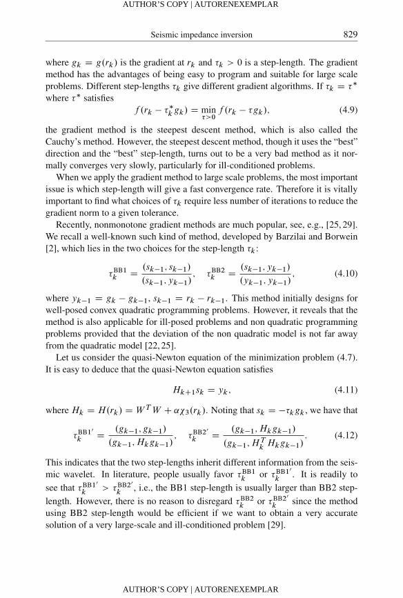
In recent communications, van den Doel and Ascher notice the chaotic nature ofthe nonmonotone gradient methods when they study the Poisson problem
��u.; t/ D q.s; t/; ; t 2 .0; 1/
solved by the nonmonotone gradient method [19]. In which, q.; t/ is known andsubject to homogeneous Dirichlet boundary conditions. The chaotic nature lies inthe sensitivity of the total number of iterations required to achieve a fixed accuracyto small changes in the initial vector 0. We give an example of 1d case:
Ax.s/ D
Z�
a.s � t /x.t/dt D z.s/;
where a.s/ D 1=.p2��/ exp.�1=2.s=�/2/, D Œ��=2; �=2� and the true solu-
tion is 2 exp.�6.t � 0:8/2/C exp.�2.t C 0:5/2/.The initial guess value is chosen as x0Da1e1Ca2e2, where ai 2 Œ�10�5; 10�5�
(i D 1; 2), e1 and e2 are two random orthogonal vectors. The chaotic nature canbe vividly seen from Figure 1.
The chaotic nature indicates that the pure nonmonotone iteration may be notsufficient to guarantee fast convergence, some safeguard techniques maybe useful.
4.3 Safeguard
From equations (4.1)–(4.2) we learn that their solution is also the solution of theproblem
min kW r � dıkl2 ; (4.14)
s.t. krkl1 � �; � > 0: (4.15)
Therefore, r� solves (4.14) within the feasible set S D ¹r W krkl1 � �º. To main-tain this property, we apply a projection technique. Note that the set S is bounded
AUTHOR’S COPY | AUTORENEXEMPLAR
AUTHOR’S COPY | AUTORENEXEMPLAR
Seismic impedance inversion 831
−5 −4 −3 −2 −1 0 1 2 3 4 5
x 10−5
60
80
100
120
140
160
180
X (coefficient)
Num
ber
of it
erat
ions
Figure 1. Chaotic nature of the nonmonotone gradient method.
below and convex, therefore, there exists a projection operator PS W RN ! S
onto S such thatPS .x/ D argminzkx � zk; z 2 S:
The projection is easy to be calculated [3]. Assume that the current iterate rk isfeasible, then the next iteration point can be obtained by
rkC1 D PS .rk � kgk/:
4.4 Choosing the regularization parameter
There are many ways to choosing the regularization parameter. Roughly speaking,the techniques can be classified as either a priori way or a posteriori way. An apriori choice of the regularization parameter ˛ requires that ˛ > 0 and is fixed.An a posteriori choice of the regularization parameter usually requires solvingnonlinear equations about ˛ which involves the computations of derivatives ofthe solution r˛ . For our gradient descent method, we apply a simple posterioritechnique, i.e., a geometric choice manner,
˛k D ˛0 � k�1; 2 .0; 1/; (4.16)
where ˛0 > 0 is a preassigned value of regularization parameter.
AUTHOR’S COPY | AUTORENEXEMPLAR
AUTHOR’S COPY | AUTORENEXEMPLAR
832 Y. Wang
4.5 Remarks
The minimization model based on combination of l2 and l1 norm possesses sev-eral advantages. A simple fact is that the l1 norm is robust to eliminate outliersand large amplitude anomalies when the necessity of the signal to have minimumenergy is unnecessary. A more general form is the lp-lq model, which can be inthe form
min f .r/ WD kW r � dıkp
lpC ˛kL.r � r0/k
q
lq; (4.17)
where p; q > 0 which are specified by users, ˛ > 0 is the regularization parame-ter, L is the scale operator and r0 is an a priori estimated solution of the originalmodel. This model relaxes the convexity requirements on the usual models l2-l2 and l2-l1. Details about implementation of the minimization model are givenin [23].
5 Numerical experiments
5.1 Synthetic simulations
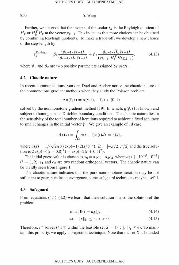
The seismogram is generated by a velocity model with 6 layers, see Figure 2. Thethickness of each layer varies. The velocity parameter in each layer is shown inTable 5.1. To generate the seismogram, a theoretical Ricker wavelet
w.t/ D .1 � 2�2f 2mt2/ exp.�.�fmt /
2/
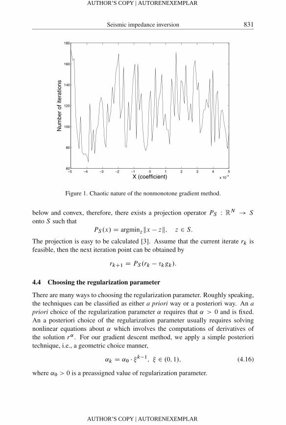
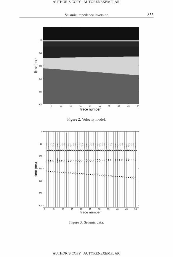
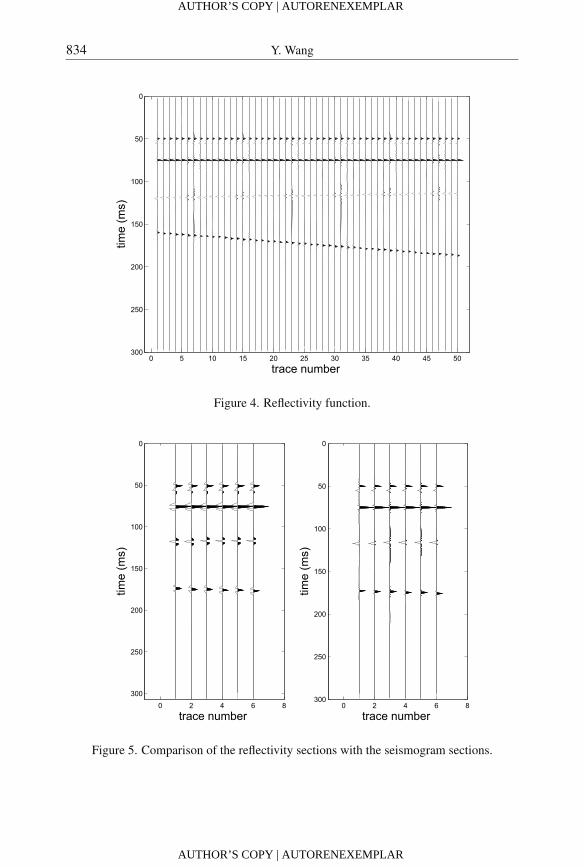
is used to perform a convolution, where fm represents the central frequency. Theseismic records with additive Gaussian random noise is shown in Figure 3. Usingour algorithm, the retrieved reflectivity function is shown in Figures 4 and 5. It isevident that our algorithm can reduce the noise and retrieve the reflectivity stably.With the reflectivity function we could rebuild the velocity. The recovered velocityis shown in Figure 6. Comparison of the true velocity model (Figure 2) with therecovered velocity (Figure 6) reveals that our algorithm is robust and could be usedfor seismic impedance inversion.
layers 1 2 3 4 5 6
V (km � s�1) 2.5 3.0 2.7 3.2 3.8 4.0
Table 1. Parameters of the velocity model.
AUTHOR’S COPY | AUTORENEXEMPLAR
AUTHOR’S COPY | AUTORENEXEMPLAR
Seismic impedance inversion 833
trace number
time
(ms)
5 10 15 20 25 30 35 40 45 50
50
100
150
200
250
300
Figure 2. Velocity model.
0 5 10 15 20 25 30 35 40 45 50
0
50
100
150
200
250
300
time
(ms)
trace number
Figure 3. Seismic data.
AUTHOR’S COPY | AUTORENEXEMPLAR
AUTHOR’S COPY | AUTORENEXEMPLAR
834 Y. Wang
0 5 10 15 20 25 30 35 40 45 50
0
50
100
150
200
250
300
time
(ms)
trace number
Figure 4. Reflectivity function.
0 2 4 6 8
0
50
100
150
200
250
300
time
(ms)
trace number0 2 4 6 8
0
50
100
150
200
250
300
time
(ms)
trace number
Figure 5. Comparison of the reflectivity sections with the seismogram sections.
AUTHOR’S COPY | AUTORENEXEMPLAR
AUTHOR’S COPY | AUTORENEXEMPLAR
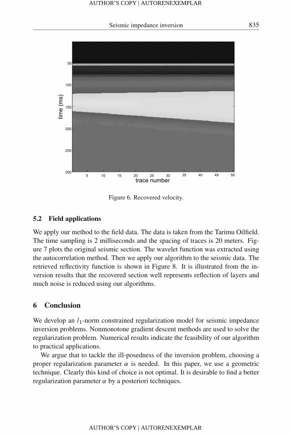
Seismic impedance inversion 835
time
(ms)
trace number5 10 15 20 25 30 35 40 45 50
50
100
150
200
250
300
Figure 6. Recovered velocity.
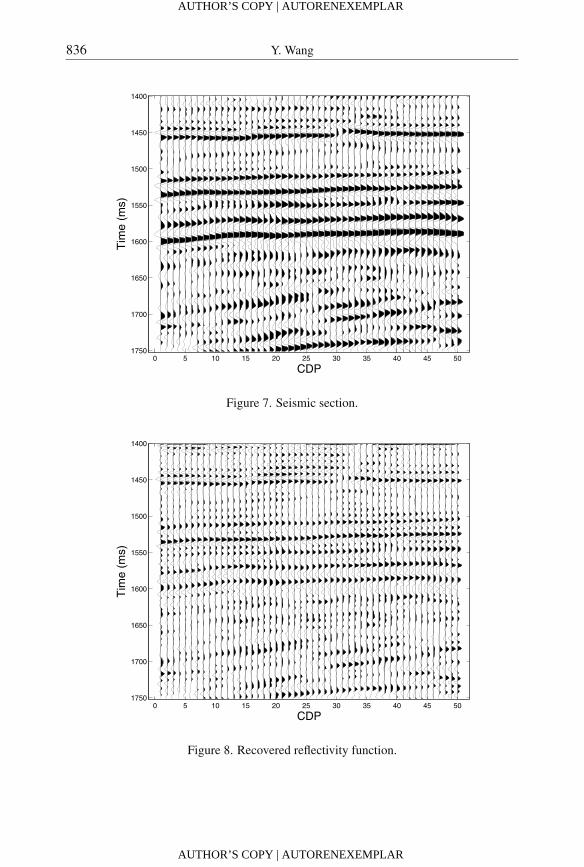
5.2 Field applications
We apply our method to the field data. The data is taken from the Tarimu Oilfield.The time sampling is 2 milliseconds and the spacing of traces is 20 meters. Fig-ure 7 plots the original seismic section. The wavelet function was extracted usingthe autocorrelation method. Then we apply our algorithm to the seismic data. Theretrieved reflectivity function is shown in Figure 8. It is illustrated from the in-version results that the recovered section well represents reflection of layers andmuch noise is reduced using our algorithms.
6 Conclusion
We develop an l1-norm constrained regularization model for seismic impedanceinversion problems. Nonmonotone gradient descent methods are used to solve theregularization problem. Numerical results indicate the feasibility of our algorithmto practical applications.
We argue that to tackle the ill-posedness of the inversion problem, choosing aproper regularization parameter ˛ is needed. In this paper, we use a geometrictechnique. Clearly this kind of choice is not optimal. It is desirable to find a betterregularization parameter ˛ by a posteriori techniques.
AUTHOR’S COPY | AUTORENEXEMPLAR
AUTHOR’S COPY | AUTORENEXEMPLAR
836 Y. Wang
0 5 10 15 20 25 30 35 40 45 50
1400
1450
1500
1550
1600
1650
1700
1750
CDP
Tim
e (m
s)
Figure 7. Seismic section.
0 5 10 15 20 25 30 35 40 45 50
1400
1450
1500
1550
1600
1650
1700
1750
CDP
Tim
e (m
s)
Figure 8. Recovered reflectivity function.
AUTHOR’S COPY | AUTORENEXEMPLAR
AUTHOR’S COPY | AUTORENEXEMPLAR
Seismic impedance inversion 837
Bibliography
[1] K. Aki and P. G. Richards, Quantitative Seismology: Theory and Methods, W. H.Freeman and Company, San Francisco, 1980.
[2] J. Barzilai and J. Borwein, Two-point step size gradient methods, IMA Journal ofNumerical Analysis, 8 (1988), 141–148.
[3] M. Bertero and P. Boccacci, Introduction to Inverse Problems in Imaging, Instituteof Physics Publishing, Bristol and Philadelphia, 1998.
[4] J. Claerbout and F. Muir, Robust modeling with erratic data, Geophysics, 38 (1973),826–844.
[5] Y. Cui , Y. F. Wang and C. C. Yang, Regularizing method with a priori knowledgefor seismic impedance inversion, Chinese Journal of Geophysics, 52 (2009), 2135–2141.
[6] V. Dimri, Deconvolution and Inverse Theory-Applications to Geophysical Problems,Elsevier, Amsterdam, 1992.
[7] D. E. Goldberg, Genetic Algorithms in Search. Optimization & Machine Learning,Addison-Wesley Publishing Company, INC, 1989.
[8] S. I. Kabanikhin, Definitions and examples of inverse and ill-posed problems, J. Inv.Ill-posed Problems, 16 (2008), 317–357.
[9] K. Levenberg, A method for the solution of certain nonlinear problems in leastsquares, Qart. Appl. Math., 2 (1944), 164–166.
[10] D. W. Marquardt, An algorithm for least-squares estimation of nonlinear inequalities,SIAM J. Appl. Math., 11 (1963), 431–441.
[11] G. Nolet, Seismic Tomography, Reidel Publishing, Boston, 1987.
[12] G. Nolet and R. Snieder, Solving large linear inverse problems by projection, Geo-phys. J. Int., 103 (1990), 565–568.
[13] A. Tarantola, Inverse Problems Theory: Methods for Data Fitting and Model Param-eter Estimation, Elsevier, Amsterdam, 1987.
[14] A. N. Tikhonov and V. Y. Arsenin, Solutions of Ill-posed Problems, John Wiley andSons, New York, 1977.
[15] A. N. Tikhonov, A. V. Goncharsky, V. V. Stepanov and A. G. Yagola, NumericalMethods for the Solution of Ill-Posed Problems, Kluwer, Dordrecht, 1995.
[16] J. Trampert and J. J. Leveque, Simultaneous iterative reconstruction technique: phys-ical interpretation based on the generalized least squares solution, Journal of Geo-physical Research, 95 (1990), 12553–12559.
[17] T. J. Ulrych, M. D. Sacchi and M. Grau, Signal and noise separation: art and science,Geophysics, 64 (1999), 1648–1656.
[18] T. J. Ulrych, M. D. Sacchi and A. Woodbury, A Bayesian tour to inversion, Geo-physics, 66 (2000), 55–69.
AUTHOR’S COPY | AUTORENEXEMPLAR
AUTHOR’S COPY | AUTORENEXEMPLAR
838 Y. Wang
[19] K. van den Doel and and U. Ascher, The chaotic nature of faster gradient descentmethods, Preprint, 2010.
[20] J. Y. Wang, Inversion Theory for Geophysics, Higher Education Press, Beijing, 2002,(in Chinese).
[21] Y. F. Wang, Computational methods for inverse problems and their applications,Higher Education Press, Beijing, 2007, (in Chinese).
[22] Y. F. Wang, An efficient gradient method for maximum entropy regularizing retrievalof atmospheric aerosol particle size distribution function, Journal of Aerosol Science,39 (2008), 305–322.
[23] Y. F. Wang, J. J. Cao, Y. X. Yuan, C. C. Yang and N. H. Xiu, Regularizing active setmethod for nonnegatively constrained ill-posed multichannel image restoration prob-lem, Applied Optics, 48 (2009), 1389–1401.
[24] Y. F. Wang, S. F. Fan and X. Feng, Retrieval of the aerosol particle size distribu-tion function by incorporating a priori information, Journal of Aerosol Science, 38(2007), 885–901.
[25] Y. F. Wang and S. Q. Ma, Projected Barzilai–Borwein methods for large scalenonnegative image restorations, Inverse Problems in Science and Engineering, 15(2007), 559–583.
[26] Y. F. Wang and C. C. Yang, Accelerating migration deconvolution using a non-monotone gradient method, Geophysics, 75 (2010), S. 131–S. 137.
[27] W. C. Yang, On inversion methods for nonlinear geophysics, Progress in Geophysics,17 (2002), 255–261, (in Chinese).
[28] O. Yilmaz, Seismic Data Processing, Investigations in Geophysics No. 2, Society ofExploration Geophysicists, Tulsa, Okla, 1987.
[29] Y. Yuan, Gradient methods for large scale convex quadratic functions, in Y. F. Wang,A. G. Yagola and C. C. Yang editors, Optimization and Regularization for Computa-tional Inverse Problems and Applications, Springer, Berlin, 2010, pp. 141–155.
[30] H. B. Zhang, Z. P. Shang and C. C. Yang, A non-linear regularized constrainedimpedance inversion, Geophysical Prospecting, 55 (2007), 819–833.
Received August 20, 2010; revised December 2, 2010.
Author information
Yanfei Wang, Key Laboratory of Petroleum Resources Research,Institute of Geology and Geophysics, Chinese Academy of Sciences,P. O. Box 9825, Beijing, 100029, P. R. China.E-mail: [email protected]
AUTHOR’S COPY | AUTORENEXEMPLAR
AUTHOR’S COPY | AUTORENEXEMPLAR


![arXiv:1706.06141v1 [math.NA] 19 Jun 2017Vatankhah et al. 3 Inversion of gravity data using the RSVD of the L 1-norm stabilizer with a L 2-norm term, and a hard constraint matrix W](https://img.pdfslide.us/doc/110x75/5e62b76cfbc9411ca23c4c19/arxiv170606141v1-mathna-19-jun-2017-vatankhah-et-al-3-inversion-of-gravity.jpg)