An Effective Method for Inversion of Elastic Impedance for ... D. Myers, Director ... 2006 Posted online January 2007 This publication is available only online at ... the inversion

U.S. Department of the InteriorU.S. Geological Survey

Scientific Investigations Report 2006–5297

An Effective Method for Inversion of Elastic Impedance for Shallow Sediments and Its Application to Gas Hydrate-Bearing Sediments

1n(1

∆k∆k

n

Q


By Myung W. Lee

Scientific Investigations Report 2006–5297

U.S. Department of the InteriorU.S. Geological Survey

U.S. Department of the InteriorDIRK KEMPTHORNE, Secretary

U.S. Geological SurveyMark D. Myers, Director

U.S. Geological Survey, Reston, Virginia: 2006

Posted online January 2007

This publication is available only online at http://pubs.usgs.gov/sir/2006/5297/

For more information on the USGS--the Federal source for science about the Earth, its natural and living resources, natural hazards, and the environment: World Wide Web: http://www.usgs.gov Telephone: 1-888-ASK-USGS

Any use of trade, product, or firm names is for descriptive purposes only and does not imply endorsement by the U.S. Government.

Although this report is in the public domain, permission must be secured from the individual copyright owners to reproduce any copyrighted materials contained within this report.

Suggested citation:Lee, M.W., 2006, An effective method for inversion of elastic impedance for shallow sediments and its application to gas hydrate-bearing sediments: U.S. Geological Survey Scientific Investigations Report 2006–5297, 11 p.

http://pubs.usgs.gov/sir/2006/5297

http://www.usgs.gov

iii

Contents

Abstract ...........................................................................................................................................................1Introduction.....................................................................................................................................................1Theory .............................................................................................................................................................2

Elastic Impedance ................................................................................................................................2Original Formulation of EI-inversion ..................................................................................................2New Formulation of EI-inversion ........................................................................................................2

Results and Analysis .....................................................................................................................................4Noiseless Input......................................................................................................................................4Noisy Input .............................................................................................................................................5Comparison Between Original Inversion and New Inversion Equations ....................................7Error in VS Associated with Error in Elastic Impedance .................................................................8Inversion for Gas Hydrate-Bearing Sediments ................................................................................8

Conclusions...................................................................................................................................................10References ....................................................................................................................................................10

Figures 1–9. Graphs showing: 1. Error analysis .........................................................................................................................3 2. Inversion results from the new formula using noiseless elastic impedance ..............4 3. Inversion results using noisy elastic impedance at the Keathley Canyon

151-2 well ................................................................................................................................5 4. Inversion results using noisy elastic impedance at the Alpine-1 well .........................6 5. Inversion results from the new formula using noisy elastic impedance .....................6 6. The S-wave velocity simulated at the Keathley-Canyon 151-2 well .............................7 7. Gain factor with respect to the fractional error in elastic impedance .........................8 8. Inversion results for gas hydrate-bearing sediments at the Keathley

Canyon 151-2 well ..................................................................................................................9 9. Inversion results for gas hydrate-bearing sediments at the Mallik 5L-38 well,

Canada ..................................................................................................................................10

AbstractElastic properties of gas hydrate-bearing sediments

(GHBS) are important for identifying and quantifying gas hydrate as well as discriminating the effects of free gas on velocity from that due to overpressure. Elastic properties of GHBS sediments can be estimated from elastic inversion using the elastic impedance. The accuracy of elastic inversion can be increased by using the predicted S-wave velocity (V

S) in the

parameter k, which is k = (VS / V

P)2. However, when V

S is less

than about 0.6 kilometer per second, the inversion is inaccu-rate, partly because of the difficulty in accurately predicting low S-wave velocities and partly because of the large error associated with small k values. A new formula that leads to estimates of only the high-frequency part of velocity is pro-posed by decomposing V

S into low- and high-frequency parts.

This new inversion formula is applied to a variety of well logs, and the results demonstrate its effectiveness for all ranges of V

S as long as the deviation of V

S from the low-frequency part

of VS is small. For GHBS, the deviation of V

S from the low-

frequency part of VS can be large for moderate to high gas

hydrate saturations. Therefore, the new formula is not effective for elastic inversion for GHBS unless the gas hydrate effect is incorporated into the low-frequency part of V

S. For inversion

of GHBS with VS greater than about 0.6 kilometer per second,

the original formulation is preferable.

IntroductionIdentification and quantification of gas hydrate present

in sediments are important research areas (Collett, 2002), and detailed seismic analysis is necessary to detect gas hydrate-bearing sediments (GHBS). Gas hydrate increases the seismic velocities of sediments; therefore, the effect manifests itself in the amplitude and traveltime of seismic data. By comparing seismically driven interval velocities to those for sediments without gas hydrate, GHBS can be identified and quanti-fied (for example, see Tinivella and Lodolo, 2000; Lu and McMechan, 2002; Jin and others, 2003).

Detailed velocity information for sediments is essential to accurately estimate the amount of gas hydrate. Arrival times provide the low-frequency velocity informa-tion, and amplitudes provide the high-frequency information of velocities. By combining the amplitude and traveltime information, detailed interval velocities can be estimated. The high-frequency part of velocity information can be deduced from the amplitude-versus-offset (AVO) intercept and gradient or elastic impedances calculated through angle stacks.

Elastic impedance (EI) is a generalization of acoustic impedance (AI) using a three-term approximation of reflec-tion coefficients (Connolly, 1999). AI has been used success-fully to derive P-wave velocities for GHBS (Sakai, 1999; Lu and McMechan, 2002; Jin and others, 2003). However, more detailed seismic-attribute analysis for GHBS can be accom-plished by estimating S-wave velocities from the seismic data using elastic inversion (Mallick and others, 2000; Lu and McMechan, 2002).

Elastic inversion can be calculated in different ways—for example, by full prestack inversion (Mallick, 1999), by post-stack inversion using AVO (AVO-inversion), and by poststack inversion using elastic impedance (EI-inversion). Although computationally expensive, the full prestack inversion is optimum for obtaining elastic parameters from seismic data. Many good results are obtained, however, by using AVO-inversion (Mallick, 2001) or EI-inversion (Lu and McMechan, 2004).

Detailed inversion methods using the elastic impedances are discussed in Lee (2006), where predicted S-wave velocities are used to increase the accuracy of inversion without assum-ing V

S / V

P = 0.5 or some constant (Connolly, 1999; Mallick

and others, 2000; Mallick, 2001). The inversion proposed by Lee (2006) is problematic, however, when V

S is less than about

0.6 kilometer per second (km/s), which is the velocity range for most GHBS in marine environments.

In this paper, a new effective formula for elastic inver-sion for low S-wave velocities (less than about 0.6 km/s) is proposed by decomposing V

S into low- and high-frequency

parts. The new formula is applied to well logs acquired at the Keathley Canyon 151-2 well, Gulf of Mexico; Alpine-1 well,


By Myung W. Lee

North Slope of Alaska; and Mallik 5L-38, western Canada, with promising results. By using the new formula for V

S less

than about 0.6 km/s and the original formula for VS greater

than about 0.6 km/s, accurate S-wave velocities for GHBS can be estimated at the Mallik 5L-38 well.

Theory

Elastic Impedance

Impedance is generally defined as a product of P-wave velocity, and density and is related to a normal-incidence reflection seismogram. However, this definition cannot be applied to far-offset data. In order to generalize the normal incidence impedance concept, Connolly (1999) defined EI as follows:

EI V Vp sk k( ) ( tan ) sin ( sin )θ ρθ θ θ= + − −1 8 1 42 2 2 (1)

with the parameter k = (VS / V

P)2. V

P, V

s, r, and q, are P-wave

velocity, S-wave velocity, density, and angle of incidence, respectively. The dimension of EI in equation 1 varies with respect to the angle of incidence. In order to avoid this dimen-sion change in EI, a normalized elastic impedance concept is used in this report (Whitcombe, 2002).

Original Formulation of EI-inversion

A detailed description of EI-inversion is given in Lee (2006). A practical way of EI-inversion is using a sequential inversion of AI and EI (Lu and McMechan, 2004; Lee, 2006). P-wave impedance is estimated from the AI-inversion using EI(0), and the shear wave-velocity is estimated from the fol-lowing equation using EI(q),

ln( )( tan ) ln( ) ln( ( )) ( sin ) ln( )

sinV

V EI kks

p=+ − + −1 1 4

8

2 2

2

θ θ θ ρθ

. (2)

EI-inversion using equation (2) requires a good estimate of k, and it is particularly important to estimate reliable S-wave velocities at shallow depths, where small k values are required.

The error associated with error in k can be derived by writing equation 2 as

ln( ) sin ln sin ln( )sin

V V Q k kk ks s+ = − −

+∆ ∆

∆4 4

8

2 2

2

θ ρ θ ρθ

(3)

where Q = (1 + tan2 q)1nVp – 1nEI(q) +1nr. When k >> Dk,

equation 3 becomes

ln ( / ) ln ln( ) (ln ln )( )V V V V V kk

kks s s s s1 1

21+ = + + ≈ − −∆ ∆ ∆ε ρ . (4)

Therefore,

ln( ) ln ln12

+ ≈ − +

ε ρV kks

∆

ε ρρ= − ≈ − +

− +e V kk

V k ks

s(ln ln / ) / ln ln2 12

∆ ∆ (5)

When Dk >> k, the error can be written as

ln( ) ln ln ln1 12

1+ = −

− − −

ε ρkk

kk

V V kks s∆ ∆ ∆

. (6)

The error of S-wave velocity associated with error in k in the case that an error in k is much larger than k itself is given by

ε ρ= −− +e Vs(ln ln / )2 1 (7)

Errors calculated from equations 5 and 7 are shown in figure 1A. When the error in k is small, the errors in the estimated S-wave velocities are also small. However, when the error in k is larger than k itself, figure 1A indicates a large error in the predicted S-wave velocity. Note that when Dk >> k, the error is independent of k and dependent only on the S-wave velocity and density of the medium. This kind of error occurs when S-wave velocities at shallow depths are estimated using EI-inversion. For example, the P- and S-wave velocities at 100-m subbottom depth are typically 1.55 km/s and 0.15 km/s, respectively. This gives a value of k of about 0.1. If k of 0.21 is used for the inversion, the error in k is about 0.2, which is 20 times larger than the true k. Assuming a density of 1.66 g/cm3, the error from equation 7, or approximately from figure 1A, is about 4, yielding the estimated V

S = 0.15 km/s × 4. = 0.6 km/s.

Therefore, inverting low S-wave velocities from the seismic data is not practical using equation 2 because the required accuracy of k may not be obtained.

Although k values can be closely estimated, the inversion is inaccurate when k is very small (less than ~0.07). Because k is in the denominator in equation 2, a small error in the input can be accentuated in the inversion results. Therefore, equa-tion 2 is not a practical approach when using EI-inversion with low S-wave velocities.

New Formulation of EI-inversion

As mentioned previously, the inversion scheme shown in equation 2 is sensitive to k. Lee (2006) suggested using a more accurate k by using predicted S-wave velocity in the inversion scheme, and this approach works well when k is greater than about 0.1 and noise is small. However, modeling indicates that this approach substantially overestimates S-wave velocity when k is very small, less than about 0.07 as in unconsolidated sediments at shallow depths. Consequently, this approach is inadequate for the elastic inversion for gas hydrate-bearing sediments at shallow depths.

� An Effective Method for Inversion of Elastic Impedance and Its Application to Gas Hydrate-Bearing Sediments

Elastic impedances consist of two components; one is a slowly varying or low-frequency component (sometimes viewed as a trend) and the other is a high-frequency compo-nent. The primary function of the low-frequency component is the kinematics of the wave field, which controls arrival times of P- and S-waves. The high-frequency components control the amplitudes of waves. Therefore, it is useful to decompose the EI into two components, and equation 1 can be written, by taking the natural logarithm and assuming that density has only a low-frequency component, as

ln ln ( ) ln( ) ( tan )[ln ln( )]

sin [ln

EI EI Vk V

LPL= + + = + + +

−

θ δ θ αθ

1 1 1

8

2

2ssL k+ + + −ln( )] ( sin ) ln( )1 1 4 2β θ ρ (8)

where a = VP

H / Vp

L, b = VSH / V

SL, d = EIH / EIL, the superscript

L is the low-frequency component, and the superscript H is the high-frequency component. The low-frequency component of EI due to the low-frequency part of V

S can be written as

ln ( ) ( tan )[ln ] sin [ln( )]

( sin ) ln(

EI V k Vk

LP L S

L

L

θ θ θθ

= + −

+ −

1 8

1 4

2 2

2 ρρ) (9)

with kL = (V

SL / V

P)2.

By subtracting the low-frequency component of elastic impedance from equation 8 using equation 9, it is shown that equation 8 becomes

ln( )ln( ) ( )sin ln( ) ( )sin ln( )

si

11 8 4

8

2 2

+ =− + − − − −

βδ θ θ ρk k V k k

kL S

LL

nn2 θ (10)

The inversion method proposed here is based on the assumption that equation 10 can be approximated by the following equation:

ln( ) ( tan ) ln( ) ln( )sin*1 1 1 1

8

2

2+ ≈ + + − +β θ α δθk

(11)

The purpose of this formulation is to mitigate the error associ-ated with small values of k in equation 2. If a large k* for small V

S can be used in equation 11 and the approximation of

equation 11 is valid, errors associated with small k values in the original formula can be reduced.

The parameter k* in equation 11 is different from the parameter k in equations 2 or 10. The k* is just a convenient parameter, and its value is chosen to yield accurate S-wave velocities from the inversion. Note that values for low-frequency components are much higher than those for high-frequency components in consolidated sediments. Therefore, in most seismic applications, a, b, and d are small numbers. However, b can be large because V

S is small at shallow depths.

Therefore, a more accurate VSL is required for the inversion of

sediments at shallow depth to reduce the magnitude of b, as shown in the next section.

The error of S-wave velocity associated with the uncertainty in k* using equation 11 when k* >> Dk* can be written as

∆ ∆∆VV

e kk

SH

S

k k= − ≈ − +− +(ln( )) /*

*

* *

ln( )1 1 1β β . (12)

Figure 1. Error analysis. A, Fractional error in VS with respect to VS for a given uncertainty in k when using the original equation, equation 2. B, Fractional error in VS with respect to parameter b (b = VS

H / VSL)

for a given uncertainty in k* when using the new equation, equation 11.

FRA

CT

ION

AL

ER

RO

R IN

VS,∆

VS

/VS

FRA

CT

ION

AL

ER

RO

R IN

VS,∆

VS

/VS

6

4

2

0

–20.0 0.5 1.0 1.5 2.0

S-WAVE VELOCITY,IN KILOMETERS PER SECOND

For a given ρ = 1.8 g/cm3

∆k / k = 0.1∆k >>k

A PARAMETER β–0.8 –0.4 0.4 0.80.0

4

6

2

0

–2

B

Error when ∆k* / k* = 0.1Error when ∆k* >> k*

Theory �

When k* << Dk*, the error becomes

∆VV

eSH

S

= −− +ln( )1 1β . (13)

Figure 1B shows calculated errors for Dk* / k* = 0.1 and Dk* >> k* with respect to the parameter b. The error increases as the magnitude of b increases, which is similar to the behav-iors shown in figure 1A. However, the magnitude of error is small if the magnitude of b is small. In other words, if the low-frequency part of the S-wave velocity is determined accurately, equation 11 yields more accurate S-wave velocities than those estimated from equation 2. Therefore, equation 11 can be used to estimate low S-wave velocities using EI-inversion if reason-able values of k*, preferably greater than 0.01, can be obtained.

Results and Analysis

Noiseless Input

Figure 2 shows the estimated S-wave velocities using noiseless EI (0) and EI (25) at the Keathley Canyon 151-2 well, Gulf of Mexico, and the Alpine-1 well, North Slope of Alaska. At the Keathley Canyon 151-2 well, there were no

measured velocities, so velocities were predicted from porosi-ties using the modified Biot-Gassmann theory by Lee (Lee, 2002), referred to as the BGTL, with the BGTL parameter m = 1.5. The calculated velocities are denoted as synthetic velocities in this paper.

In order to estimate a reasonable k* for equation 11, a series of inversions using different values of k* was performed

and k* was chosen based on the accuracy of estimated S-wave velocities. This exercise resulted in the following values of k*: k* = 0.1 when V

SL <0.2 km/s, k* = 0.15 when V

SL < 0.4 km/s,

k* = 1.0 when VS

L > 1.5 km/s, and k* is linearly interpolated between 0.15 and 1.0 when 0.4 < V

SL < 1.5 km/s. The red dot-

ted lines in figure 2 show S-wave velocities estimated from equation 11 with these k*values. As indicated, the inverted S-wave velocities using equation 11 are similar to input S-wave velocities for V

S greater than about 0.25 km/s. Note

that all inversion results, unless stated, were smoothed using 11 points.

S-wave velocities less than about 0.25 km/s, shown in figure 2A, are not accurate. The smallest k* used in the inver-sion is 0.1. In order to estimate very small S-wave velocities accurately, k* should be much smaller than 0.1. Small values of k*, however, yield large errors in S-wave velocities. As will be discussed, the error can be reduced by using the more accu-rate low-frequency part of V

S. The advantage of the new for-

mula is its ability to reduce errors by using the more accurate

Figure �. Inversion results from the new formula using noiseless elastic impedance calculated at an incidence angle of 25°. A, At the Keathley Canyon 151-2 well, Gulf of Mexico. The synthetic velocity is the predicted S-wave velocity from porosity. B, At the Aline-1 well, North Slope of Alaska.

Keathley Canyon 151-2 well Alpine-1 well

A B DEPTH, IN FEETSUBBOTTOM DEPTH, IN METERS

S-W

AV

E V

ELO

CIT

Y, IN

KIL

OM

ET

ER

S P

ER

SE

CO

ND

S-W

AV

E V

ELO

CIT

Y, IN

KIL

OM

ET

ER

S P

ER

SE

CO

ND

0.8

0.4

0.00 250 500 2,000 4,000 6,000

2.0

1.5

1.0

0.5

Measured velocityUsing the original equationUsing the new equation

Synthetic velocityUsing the original equationUsing the new equation


low-frequency part of S-wave velocity without decreasing the k* value for small values of V

S. The original formula is inde-

pendent of the low-frequency part of the S-wave velocity.For comparison, the inversion results using the original

equation 2 is shown as blue lines in figure 2. For S-wave velocities less than about 0.6 km/s, the inversion results using the original equation are inferior to those from the new equa-tion, whereas the results are similar for S-wave velocities greater than about 0.6 km/s.

The accurate inversion results using equation 2 for V

S > 0.6 km/s are due to accurate k values in the inversion,

which are possible because the predicted S-wave velocities were used in calculating k, as demonstrated in Lee (2006). The inac-curacy of inversion results using equation 2 for V

S <0.6 km/s is

due to the inability of obtaining accurate S-wave velocities suit-able for the calculation of k as well as a small k value.

The accuracy of inversion using equation 2 can be increased with accurate k values, whereas the accuracy of inversion using equation 11 is obtained with an accurate low-frequency part of S-wave velocity or with a smaller b. In ap-plying equation 11, much simpler k* values were estimated and applied instead of using the predicted S-wave velocity. The smallest value of k* used for equation 11 is 0.15. Therefore, the inverted S-wave velocities using equation 11 at shallow depths are more stable than those estimated from equation 2, as demonstrated in figure 2A.

Noisy Input

Figure 3A shows the noiseless EI(25) and noisy EI(25) at the KC 151-2 well. The noisy EI(25) is generated by adding 10 percent random noises to the noiseless EI(25). Figure 3B shows the inversion results using equations 2 and 11. The S-wave velocities estimated using equation 2 are much larger than the input velocities when S-wave velocities are less than about 0.4 km/s. Also, local variations of S-wave velocities estimated from equation 2 are much larger than those of the input data. However, the estimated S-wave velocities using equation 11 are similar to the input data and are close to the result of noiseless input.

Another example is given in figure 4 for the Alpine-1 well. In this case, the random noise is about 20 percent. The estimated S-wave velocities using equations 2 and 11 are similar and close to measured velocities at the well. The random noise effect on the EI-inversion using the original equation is not much affected when the S-wave velocities are greater than 0.7 km/s.

For the case where the error in EI is not random noise, the inversion results are shown in figure 5. The dotted line in figure 5A shows the inverted S-wave velocity at the KC 151-2 well using equation 11 when DEI / EI = 0.1, and figure 5B shows the inverted S-wave velocity at the Alpine-1 well when DEI / EI = 0.5. Figure 5 indicates that the inverted S-wave velocities using equation 11 are shifted more toward lower velocities than measured S-wave velocities. However, the local

Figure �. Inversion results using noisy elastic impedance (EI) calculated at an incidence angle of 25° at the Keathley Canyon 151-2 well. A, Noiseless EI(25) with a black line and noisy EI(25) with green line. B, Inversion results using the original and new formulas.

0 250 500

5

4

3

2

SUBBOTTOM DEPTH, IN METERS

ELA

ST

IC IM

PE

DA

NC

E, E

(25)

Keathley Canyon 151-2 well

A B

0.8

0.6

0.4

0.2

0.00 250 500


S-W

AV

E V

ELO

CIT

Y, IN

KIL

OM

ET

ER

S P

ER

SE

CO

ND

Noisy data EI(25) inversionSimulated velocityVelocity using the original equationVelocity using the new equation

Noiseless EI(25)Noisy EI(25) (about 10 percent random noise)

Results and Analysis �

Figure �. Inversion results using noisy elastic impedance (EI) calculated at an incidence angle of 25° at the Alpine-1 well. A, Noiseless EI(25) with a black line and noisy EI(25) with a green line, B, Inversion results using the original and new formulas.

Figure �. Inversion results from the new formula using noisy elastic impedance (EI). A, Inversion results at the Keathley Canyon 151-2 well in the case that the fractional error in EI is 10 percent. B, Inversion results at the Alpine-1 well in the case that the fractional error in EI is 50 percent.

Noiseless EI(25)Noisy EI(25) (about 20 percent random noise)

Alpine-1 well

Noisy EI(25) inversionMeasured velocityVelocity using the original equationVelocity using the new equation

ELA

ST

IC IM

PE

DA

NC

E, E

I(25

)

12

8

4

2,000 4,000 6,000

DEPTH, TO FEET

S-W

AV

E V

ELO

CIT

Y, IN

KIL

OM

ET

ER

S P

ER

SE

CO

ND

2.0

1.5

1.0

0.52,000 4,000 6,000

DEPTH, IN FEETA B

Keathley Canyon 151-2 well Alpine-1 well

S-W

AV

E V

ELO

CIT

Y, IN

KIL

OM

ET

ER

S P

ER

SE

CO

ND


S-W

AVE

VELO

CITY

, IN

KIL

OMET

ERS

PER

SECO

ND

DEPTH, IN FEET

2.4

1.6

0.8

0.02,000 4,000 6,000 8,0000 250 500

0.8

0.4

0.0

Error in EI: 10 percentSynthetic velocityEI-inversion using the new equationEI-inversion using the new equation with matching average

Error in EI: 50 percentMeasured at Alpine-1 wellEI-inversion using the new equationEI-inversion using the new equation with matching average

A B


variations of inverted S-wave velocities are similar to those of the measured S-wave velocities. Therefore, a correction term can be estimated by assuming that an average of inverted S-wave velocities is the same as an average of low-frequency part of S-wave velocities. The red lines in figure 5 are inverted S-wave velocities determined by matching the average S-wave velocities.

Comparison Between Original Inversion and New Inversion Equations

The original inversion formulation, equation 2, works well when S-wave velocity is greater than about 0.6 km/s or k is greater than about 0.1. However, the performance deterio-rates when S-wave velocity is less than about 0.6 km/s.

As shown in figure 1A, the fractional error in the S-wave velocity due to a large error in k is large when V

S is less than

about 0.6 km/s, whereas the error associated with a large error in k* is much smaller when b is small. The smallest k* used in the inversion for figure 1A is 0.1, whereas the smallest k used is 0.01. Equations 2 and 11 indicate that the S-wave velocity is inversely proportional to k or k*. Therefore, unless exact input and k are available, the fractional error in V

S increases

as k and k* become smaller. The inversion method of the new formulation is stable because k* is greater than 0.1.

Figures 2 and 3 indicate that both inversion formulations fail to estimate S-wave velocities less than about 0.25 km/s. The P-wave velocity of water-saturated sediments is generally greater than 1.5 km/s. If it is assumed that the P-wave velocity is about 1.5 km/s for sediments whose S-wave velocities are less than 0.25 km/s, then the k value is less than about 0.03. For small val-ues of k, a small error in k corresponds to a large fractional error in k. When V

S is less than about 0.2 km/s, the predicted S-wave

velocities are much higher than the measured velocities, yielding a large error in k. Therefore, it is not practical to use equation 2 for small S-wave velocities.

The failure of equation 11 for small values of S-wave velocity is partly due to its inaccuracy and partly due to the inaccuracy of the low-frequency part of V

S. Figure 6A

shows the input S-wave velocity and low-frequency part of S-wave velocity (V

SL ) used in the inversion. Previous results

are produced using the VSL shown as LSF1 in figure 6A.

Inversion results with the VS

L using LSF2 for depths up to 40 m and LSF1 for depths greater than 40 m are shown in figure 6B. Use of the new formula leads to more reliable estimates of S-wave velocities, whereas the original for-mula fails to estimate low S-wave velocities. Therefore, for low S-wave velocities, accurate V

SL improves the accuracy

of inversion using the new formula, but not for the original formula.

Figure �. A, The S-wave velocity simulated at the Keathley-Canyon 151-2 well and low-frequency parts of S-wave velocity used in the inversion; previous results are estimated using the least-squares fit (LSF), LSF1, for all depths. B, Inversion results using the new low-frequency part of S-wave velocities shown in figure 6A. The new low-frequency part of S-wave velocity is LSF2 for depths less than 40 meters and is LSF1 for depths greater than 40 meters.


S-W

AV

E V

ELO

CIT

Y, IN

KIL

OM

ET

ER

S P

ER

SE

CO

ND

S-W

AV

E V

ELO

CIT

Y, IN

KIL

OM

ET

ER

S P

ER

SE

CO

ND

SUBBOTTOM DEPTH, IN METERS SUBBOTTOM DEPTH, IN METERS

0.8

0.4

0.00 250 500

0.8

0.4

0.00 250 500

Noise free EISynthetic velocityInversion using the original formulaInversion using the new formula

Syntheticvelocity

LFS1

LSF2

A B

Low-frequencypart of VS


The effect of VS

L on the EI-inversion can be analyzed from the error analysis shown in figure 1. In the original for-mulation, only k values control the accuracy of the inversion. As indicated previously, the desired accuracy of k may not be obtained in practice and a small error can be accentuated for low values of k. However, in the new formulation, error is dependent upon b. Therefore, by using an accurate V

SL, the

accuracy of inversion can be increased, even where there are large uncertainties in k*.

One problem in using the new equation is that the magnitude of parameter b should be small to estimate accurate S-wave velocities. In other words, the new equation requires accurate low-frequency part of S-wave velocity. Because of this requirement on b, the new equation is not optimum for the inversion of GHBS as demonstrated in a later section, “Inversion for Gas Hydrate-Bearing Sediments.”

Error in VS Associated with Error in Elastic Impedance

If there is error only in EI, that is EI ⇒ EI + DEI = EI(1 + DEI / EI) = (1 + l)EI, the fractional error in V

S (e) can

be written as

ελθ= −

− +

e kln( )

sin1

8 2 1, (14a)

and ελθ= −

− +

e kln( )

sin*1

8 2 1. (14b)

Equations 14a and 14b are respective errors that occur when the original and the new equations are used. The S-wave velocity for a given error in EI is given by V

S* = V

S (1 + e),

where VS

* and VS are the erroneous and true S-wave velocities,

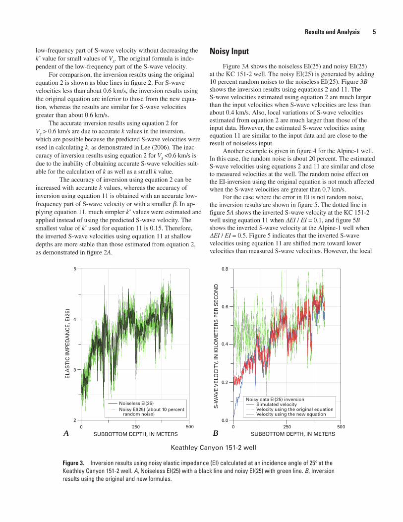
respectively.Figure 7 shows the gain factor (G), defined as G =

(1 + e), with respect to fractional errors in EI for various k or k* values. The plot indicates that inverted S-wave velocities are less than the true S-wave velocities when the fractional error in EI is greater than 0.0. The fractional error in V

S increases as

k or k* decreases. Because k values for the original formula-tion can be much less than 0.2, the fractional errors in V

S can

be large for low S-wave velocities. However, as shown in the model study, the scaling error in EI can be reduced by match-ing the average S-wave velocities between the low-frequency input and inverted S-wave velocities.

Inversion for Gas Hydrate-Bearing Sediments

The S-wave velocities for GHBS and host sediments can be very small as demonstrated at the Hydrate Ridge, Offshore Oregon, by Kumar and others (2006). Their S-wave velocities estimated from multicomponent ocean-bottom seismograph data are in the range of 0.15 to 0.35 km/s. Also, S-wave

velocities analyzed from the multicomponent ocean-bottom cable data in the Gulf of Mexico by Hardage and others (2006) are in the range of 0.3 km/s. The well log S-wave velocities of GHBS at Hydrate Ridge that were acquired during Ocean Drilling Program Leg 204 vary from 0.25 km/s to 0.65 km/s. However, S-wave velocities of GHBS at the Mallik 5L-38 well site, Mackenzie Delta, Canada, reach 2 km/s. Therefore, in order to perform EI-inversion for GHBS, all ranges of S-wave velocities should be considered.

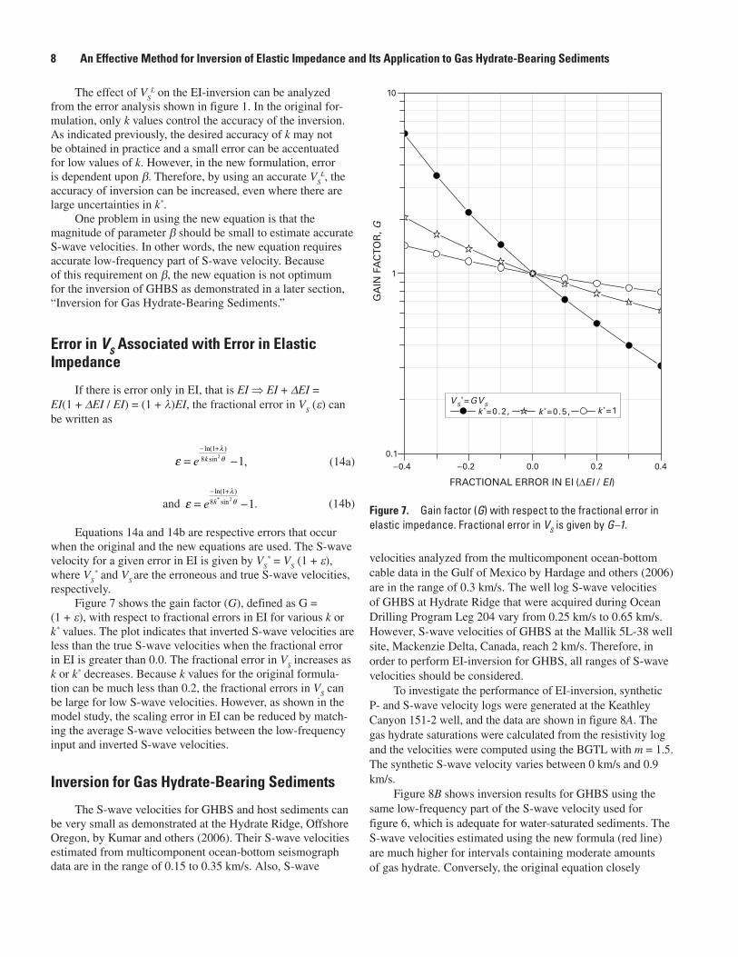
To investigate the performance of EI-inversion, synthetic P- and S-wave velocity logs were generated at the Keathley Canyon 151-2 well, and the data are shown in figure 8A. The gas hydrate saturations were calculated from the resistivity log and the velocities were computed using the BGTL with m = 1.5. The synthetic S-wave velocity varies between 0 km/s and 0.9 km/s.

Figure 8B shows inversion results for GHBS using the same low-frequency part of the S-wave velocity used for figure 6, which is adequate for water-saturated sediments. The S-wave velocities estimated using the new formula (red line) are much higher for intervals containing moderate amounts of gas hydrate. Conversely, the original equation closely

Figure �. Gain factor (G) with respect to the fractional error in elastic impedance. Fractional error in VS is given by G–1.

FRACTIONAL ERROR IN EI ( EI / EI)

GA

IN F

AC

TOR

, G

10

1

0.1–0.4 –0.2 0.0 0.2 0.4

VS*=GVS

k *=0.2, k *=0.5, k *=1


estimates S-wave velocities for GHBS near 250 m below sea floor (mbsf) (black dotted line). However, like the previ-ous example, the original equation overestimates the S-wave velocities at shallow depths where velocities are less than about 0.4 km/s.

The amount of error in S-wave velocities estimated from the new formula can be assessed using the parameter b. The V

SL near 220 mbsf is 0.43 km/s, whereas V

S is about 0.9 km/s.

Therefore, b near 220 mbsf is 1.0. Because the new equa-tion 11 is accurate for small b, the estimated S-wave velocity near 220 mbsf is inaccurate. Gas hydrate in the pore spaces increases P- and S-wave velocities significantly for moder-ate to high gas saturations, so b for GHBS can be very large unless the gas hydrate effect on velocity is incorporated in the V

SL.

The results shown in figure 8 indicate a probable opti-mum approach applicable for the inversion of GHBS at shal-low depths. It is proposed that the new formulation be used when V

SL is less than 0.4 km/s and the original equation be

used when VSL is greater than 0.4 km/s. The blue line in fig-

ure 8C shows S-wave velocities estimated from the proposed method by combining the two equations. Almost the same results are obtained if the new equation is used when k is less than 0.07 and the original equation is used when k is greater than 0.07. Using k is preferable to using V

SL to determine when

to use the new equation or the original equation because k is estimated from the input data.

It is emphasized that the largest k values appropriate for GHBS are limited by the unconsolidated nature of GHBS (Lee and Collett, 2001). Because they are unconsolidated

even at high gas hydrate saturations (Lee and Collett, 2001), the values of k for GHBS rarely exceed 0.25 (that is V

S / V

P

ratio of 0.5). When predicting S-wave velocity from P-wave velocity, it is generally assumed that the pore space is filled by water not by gas hydrate. Therefore, the predicted S-wave velocities for highly saturated GHBS are much higher than the actual velocity and yield higher k values for the inversion.

Figure 9A shows the measured P- and S-wave veloci-ties at the Mallik 5L-38 well and the calculated gas hydrate saturations from the nuclear magneto resonance porosity. As indicated, gas hydrate saturations in some intervals reach about 80–90 percent. Figure 9B shows the inverted S-wave velocities with k calculated from the predicted S-wave veloc-ity assuming 100-percent water saturation. The estimated S-wave velocities for intervals with high measured S-wave velocities (or high gas hydrate saturation) are highly under-estimated because higher values of k than actual k were used in the inversion. Therefore, it is erroneous to use predicted S-wave velocity for the inversion for highly saturated GHBS unless the effects of gas hydrate in the S-wave velocities are accounted for.

On the basis of an analysis by Lee and Collett (2001), the actual k appropriate for highly saturated GHBS is about 0.22. Figure 9C shows the inversion result by setting k = 0.22, if the calculated k values are larger than 0.22. The S-wave veloci-ties shown in figure 9C indicate that EI-inversion by limiting the maximum value of k to k = 0.22 produces accurate S-wave velocities at the Mallik 5L-38 well.

Figure �. Inversion results for gas hydrate-bearing sediments at the Keathley Canyon 151-2 well. A, Synthetic P- and S-wave velocities predicted from porosity and gas hydrate saturations estimated from the resistivity log using the modified Biot-Gassmann theory by Lee (2002). B, S-wave velocities estimated from the new and original equations. C, S-wave velocities estimated from the proposed inversion method for gas hydrate-bearing sediments.


SUBBOTTOM DEPTH, IN METERS SUBBOTTOM DEPTH, IN METERS SUBBOTTOM DEPTH, IN METERS

VE

LOC

ITY,

IN K

ILO

ME

TE

RS

PE

R S

EC

ON

D

GA

S H

YD

RA

TE

SA

TU

RA

TIO

N, I

N F

RA

CT

ION

S

2.5

2.0

1.5

1.0

0.5

0.0

0 250 500 0 250 500 0 250 500

2.5

2.0

1.5

1.0

0.5

0.0

S-wave

A B C

S-W

AV

E V

ELO

CIT

Y, IN

KIL

OM

ET

ER

S P

ER

SE

CO

ND

S-W

AV

E V

ELO

CIT

Y, IN

KIL

OM

ET

ER

S P

ER

SE

CO

ND

1.2

0.8

0.4

0.0

1.0

0.5

0.0

Synthetic velocityUsing both equations

SimulatedUsing the original equationUsing the new equation

Saturation

P-wave


ConclusionsInversion of elastic impedance is problematic when

S-wave velocities are smaller than about 0.6 km/s. The origi-nal inversion formulation requires an accurate estimate of the parameter k. It is not practical, however, to obtain the accuracy required for the inversion when S-wave velocities are less than about 0.6 km/s. In order to mitigate this problem, the S-wave velocities are decomposed into the low-frequency (input) and high-frequency (inversion result) parts with appropriate low- and high-frequency parts of elastic impedances. Using low- and high-frequency parts, a new inversion formula is derived with a new parameter k*. This new inversion formula is an approximate solution of the original inversion formula, and k* can be large, ranging from 0.1 to 1.0 depending on the S-wave velocity. For S-wave velocities less than about 0.6 km/s, the new equation appears to be appropriate.

This new inversion formula was applied to well logs acquired in the Gulf of Mexico and the North Slope of Alaska. Inversion results indicate that this new formula yields accu-rate S-wave velocities. When S-wave velocities are greater than about 0.6 km/s, both inversion methods yield accurate S-wave velocities. However, on the basis of model results, it is observed that the effect of noise in EI is less affected on the results from the new formula when S-wave velocities are less than about 0.6 km/s.

The accuracy of the new inversion equation can be increased by using an accurate low-frequency part of the S-wave velocity, even in the case that there are large uncertain-ties in k*.

For low S-wave velocities less than about 0.2 km/s, an accurate V

SL enables the new formula to estimate accurate

S-wave velocity, whereas it fails to enable the original formula to increase the inversion accuracy. However, the new equation requires a rather accurate low-frequency part of the S-wave velocity. Because of this restriction on the low-frequency part of S-wave velocity, the new equation is not adequate for inver-sion for GHBS with moderate or high gas hydrate saturations. For inversion of GHBS, using the original equation when k is greater than 0.07 and using the new equation when k is less than 0.07 appears to be appropriate. However, because GHBS is unconsolidated, the permissible largest k value is about 0.22.

References

Collett, T.S., 2002, Energy resources potential of natural gas hydrates: American Association of Petroleum Geologists Bulletin, v. 86, p. 1971–1992.

Connolly, Patrick, 1999, Elastic impedance: The Leading Edge, v. 18, p. 438–452.

Hardage, B.A., Muray, Paul, Sava, Diana, Backus, M.M., and Graebner, Robert, 2006, Evaluation of deepwater gas hydrate systems: The Leading Edge, v. 25, p. 572–576.

Jin, Y.K., Lee, M.W., Kim, Y., Nam, S.H., and Kim, K.J., 2003, Gas hydrate volume estimations on the south Shetland continental margin, Antarctic Peninsula: Antarctic Science, v. 15, p. 271–282.

Figure �. Inversion results for gas hydrate-bearing sediments at the Mallik 5L-38 well, Canada. A, Measured P- and S-wave velocities and gas hydrate saturations estimated from the nuclear magneto resonance porosity. B, Inversion results using the original equation without limiting the calculated k values. C, Inversion results using the original equation with limiting the calculated k values to 0.22, which means that the largest k value used in the inversion is 0.22.

Mallik 5L-38 well

VE

LOC

ITY,

IN K

ILO

ME

TE

RS

PE

R S

EC

ON

D

DEPTH, IN METERS DEPTH, IN METERS DEPTH, IN METERS

S-W

AV

E V

ELO

CIT

Y, IN

KIL

OM

ET

ER

S P

ER

SE

CO

ND

S-W

AV

E V

ELO

CIT

Y, IN

KIL

OM

ET

ER

S P

ER

SE

CO

ND

900900900

0

1

2

3

4

950950950 1,0001,0001,000 1,0501,0501,050

1.8

1.2

0.6

1.8

1.2

0.6

GA

S H

YD

RA

TE

SA

TU

RA

TIO

N, I

N F

RA

CT

ION

S

4

3

2

1

0

Saturation

Measured at Mallik 5L-38Estimated from EI-inversion

Measured at Mallik 5L-38Estimated from EI-inversion with kmax = 0.22

CBA

P-wave

S-wave

10 An Effective Method for Inversion of Elastic Impedance and Its Application to Gas Hydrate-Bearing Sediments

Kumar Dhananjay, Sen, M.K., and Bang, N.L., 2006, Seismic characteristics of gas hydrates at Hydrate Ridge, offshore Oregon: The Leading Edge, v. 25, p. 610–612, 614.

Lee, M.W., 2002, Modified Biot-Gassmann theory for cal-culating elastic velocities for unconsolidated and consoli-dated sediments: Marine Geophysical Researches, v. 23, p. 403–412.

Lee, M.W., 2006, Inversion of elastic impedances for uncon-solidated sediments: U.S. Geological Survey Scientific Investigations Report 2006–5081, 14 p.

Lee, M.W., and Collett, T.S., 2001, Elastic properties of gas hydrate-bearing sediments: Geophysics, v. 66, p. 763–771.

Lu, Shaoming, and McMechan, G.A., 2002, Estimation of gas hydrate and free gas saturation, concentration, and distribu-tion from seismic data: Geophysics, v. 67, p. 582–593.

Lu, Shaoming, and McMechan, G.A., 2004, Elastic impedance inversion of multichannel seismic data from unconsolidated sediments containing gas hydrate and free gas: Geophysics, v. 69, p. 164–179.

Mallick, Subhashis, 1999, Some practical aspects on imple-mentation of pre-stack waveform inversion using a genetic algorithm—An example from east Texas Woodbine gas sand: Geophysics, v. 64, p. 326–336.

Mallick, Subhashis, 2001, AVO and elastic impedance: The Leading Edge, v. 20, p. 1094–1104.

Mallick, Subhashis, Huang, X., Lauve, J., and Ahmad, R., 2000, Hybrid seismic inversion–A reconnaissance tool for deepwater exploration: The Leading Edge, v. 19, p. 1230–1251.

Sakai, A., 1999, Velocity analysis of vertical seismic pro-file (VSP) survey at JAPEX/NOC/GSC Mallik 2L-38 gas hydrate research well, and related problems for estimating gas hydrate concentration, in Dallimore, S.R., Uchida, T., and Collett, T.S., eds., Scientific results from JAPEX/JNOC/GSC Mallik 2L-38 Gas Hydrate Research Well, Mackenzie Delta, Northwest Territories, Canada: Geological Survey of Canada Bulletin 544, p. 323–340.

Tinivella, Umberta, and Lodolo, Emanuele, 2000, The Blake Ridge bottom-simulating reflector transect—Tomographic velocity field and theoretical model to estimate methane hydrate quantities, in Paull, C.K., Matsumoto, R., Wallace, P.J., and Dillon, W.P., eds., Proceedings of the Ocean Drill-ing Program, Scientific Results, v. 164: College Station, Texas A&M University, p. 273–281.

Whitcombe, D.N., 2002, Elastic impedance normalization: Geophysics, v. 67, p. 60–62.

References 11

Documents

An Effective Method for Inversion of Elastic Impedance for ... D. Myers, Director ... 2006 Posted online January 2007 This publication is available only online at ... the inversion