Embed Size (px)
Citation preview

Seismic Early Warning Systems: Procedure for Automated Decision Making
Seis
mic
Early
War
ning
Syst
ems:
Ve
roni
ca F
. Gra
sso
Proc
edur
e fo
rAut
omat
edD
ecis
ion
Mak
ing
Dot
tora
to d
i Ric
erca
in R
isch
io S
ism
ico
Università degli Studi di Napoli Federico II
Veronica Francesca Grasso
ˆPGA
PGA
Missed Alarms
False Alarms
ac ⋅
a

“Nel Mondo nulla di grande è stato fatto senza passione”
Hegel


Acknowledgments First of all I want to thank Gaetano Manfredi, Edoardo Cosenza and Paolo Gasparini that inspired
this work and supported me since my university studies. Their influence and thinking has greatly
influenced my perspectives in research and life.
I want to thank my advisor during my stay at CalTech, James Beck, for introducing me to the
exciting world of probability and Bayes theory and for being so generous with his time and ideas. I
will never forget our extremely interesting and fulfilling meetings and his lovely dedition to
transmitting all his knowledge to his students.
Special thanks to Hiroo Kanamori for encouraging my work at CalTech and for all the wise advises.
To Thomas Heaton for sharing experiences and insights on early warning throughout the
development of my work in CalTech.
To Richard Allen that with his enthusiasm in research let the work at the Seismological Lab at
University of Berkeley be an exciting experience. Collaborating with Richard provided a renew
sense of excitement for my research.
Thank you to Judith Mitrani-Reiser that was always ready to help me and let me feel at home while
in Pasadena. Thanks to Cristina Spizzuoco, Antonio Occhiuzzi, Iunio Iervolino and all my
colleagues and friends in Naples, in CalTech and in Berkeley, Ada Biondi, Tiziana Petti, Rossella
Maione and Laura Multari. I want to thank Georgia Cua for the time she dedicated me discussing on
early warning systems, one of our common interests. To Alexandra Olaya-Castro and Cristina
Nardone, my housemates in Pasadena and Berkeley respectively, with whom I share colorful and
happy memories.
Thanks to Francesco that always supported me during this great adventure that has been Ph.D.
His love and care always helped me especially away from home. Thanks for bringing love and joy
to my life.
To my sisters, Ludovica and Lucrezia, that full my life with love and joy, they are a very important
part of my life. To my mother that always supports me and is there whenever I need. Her view of
life opened my mind. To my father teaching me moderation, rationality and ambition. Thanks to
him I always remember “sky is the limit” that helps to look ahead and to remind to do the best in
every situation. To my grandmothers and grandfathers for teaching me with their example that
sacrifice and dedition pay back.
To Fabiana Piscitelli reminding me that a smile always helps.
Finally thanks to myself that realized all this.

Index Seismic early warning systems: procedure for automated decision making....…………………….1 1. Introduction.....................................................................…………………………………………1
1.1. Considerations and Road Map................................………………………………………….2 2. EWS: State-of-art............................................................…………………………………………3
2.1. Early Warning Systems...........................................………………………………………….4 2.2. Existing EWS applications......................................………………………………………….5 2.3. Innovative EWS applications: Structural Control...…………………………………………12 2.4. Prediction Methods: examples................................…………………………………………13
2.4.1. ElarmS.............................................................……………………………………….…13 2.4.2. VS method......................................................………………………………………….15
3. Seismic EWS from user’s perspective............................………………………………………...16
3.1. Time required for security measure activation.......…………………………………………17 3.2. Main aspects of consequences of prediction uncertainty.......………………………………18 3.3. Definitions...............................................................…………………………………………19
4. Uncertainty Analysis …………………………………………………………………………….23
4.1. EWS prediction process and predictors..................………………………………………….23 4.2. Uncertainty Analysis...............................................………………………………………….25
4.2.1. Sources of uncertainty.....................................…………………………………………..26 4.3. Uncertainty propagation..........................................………………………………………….27 4.4. Aproximation method for uncertainty propagation…………………………………………..28 4.5. Monte Carlo method for Uncertainty Analysis.......………………………………………….29 4.6. Monte Carlo method: quantifying ElarmS prediction error...………………………………..30
4.6.1. ElarmS Magnitude uncertainty.......................…………………………………………...31 4.6.2. Location Uncertainty.......................................…………………………………………...35 4.6.3. Attenuation model uncertainty........................……………………………………………36 4.6.4. Total Error.......................................................……………………………………………37 4.6.5. Sensitivity analysis..........................................……………………………………………40
5. Aspects of Feasibility and Reliability of Seismic EWS……………………………………………44
5.1. Probability of wrong decisions in a pre-installation scenario………………………………….44 5.2. Procedure for estimating Pfa and Pma in a pre-installation scenario.……………………………46 5.3. Prior information: Hazard function.........................……………………………………………47 5.4. Probability of false alarm in a pre-installation scenario.......…………………………………...48 5.5. Probability of missed alarm in a pre-installation scenario.....………………………………….50
6. Warning threshold design and Feasibility assessment....……………………………………………53
6.1. Designing the test procedure: warning threshold setting.......…………………………………..53 6.2. Threshold setting based on OC function.................…………………………………………….54 6.3. Threshold setting based on cost-benefit considerations.........…………………………………..56 6.4. Threshold design and Feasibility assessment: an example for Southern California …………...59

7. Operational aspects of EWS: Decision making ..............……………………………………………66 7.1. Sequential test .........................................................…………………………………………….66 7.2. Operational aspects of EWS ..........……………………………………………………………..67 7.3. Probability of wrong decisions in a real-time analysis ..........…………………………………..69 7.4. How EWS works during the event ..........................……………………………………………70 7.5. Decision making during the event ..........................………………………………………….…72 7.6. Decision making during a seismic event: simulation of the decision procedure during California Earthquakes .......................................................…………………………………………………….74
7.6.1. Yorba Linda M=4.75 ......................................……………………………………………..74 7.6.2. San Simeon M=6.5 ..........................................………………………………………….….79
7.7. Extension to other predictors than IM .....................…………………………………………….83 8. Performance-Based Earthquake Early Warning-PBEEW…………………………………………...85 8.1. PBEEW for performance assessment and design: Background ………………………………..85
8.2. PBEEW for performance assessment and design ...……………………………….……………86 8.3. PBEEW for Real-Time Loss estimation: Background ..…………………………………….….87
8.3.1. An overview .................................................……………….………………………….…...88 8.4. PBEEW for Real-Time Loss estimation .............………………..……………………………...89
9. Conclusions and Future Directions……………………...…………………………………………...93 10. References……………………………………………...…………………………………………...94

Chapter1- Introduction 1
Seismic early warning systems: procedure for automated decision
making
Veronica Francesca Grasso
Chapter 1
1. Introduction
The high social and economical relevance of the seismic risk associated with the high vulnerability
of urbanized areas has become evident in recent years due to severe losses as a consequence of
catastrophic seismic events. A detailed analysis of structural damages and economic losses due to
catastrophic events underlines the strong necessity of social, political and scientific cooperation for
disaster prevention. Historical lessons are of some help to point out the evidence that timely
warning could mitigate the effects of natural disasters.
In the recent Asian tsunami disaster occurring on 26 December 2004, thousands of lives could have
been saved if a preventive alarm and prediction had been effective, in terms of warning time and
reliability, to warn the people about the coming event. At the moment the earthquake occurred in
Sumatra, alarm messages could have been sent to the endangered areas. By the time the tsunami
arrived, many people might have been able to escape from the coastal areas, reaching higher
locations. In addition, the availability of inundation and damage maps in the few minutes after the
seismic event could have saved many other people by effective and immediate emergency aid, if an
emergency response system was in place.
Early warning technologies are a key component for an effective and efficient protection from
catastrophic natural disasters, seconds before, during and after the event (Wieland, 2001).
Early warning systems (EWS) have been recently developed as an innovative technology for natural
risk mitigation that could be applied to all natural disasters, altough the attention here is focused on
seismic risk mitigation. Effective early warning technologies for earthquakes are much more
challenging to develop because warning times range from only a few seconds to a minute or so
(Allen and Kanamori, 2003). In areas close to faults, where seismic EWS represent a mandatory
necessity, only tens of seconds of warning are available. Such short warning time means that to be
effective, a seismic EWS must depend on automated procedures, including those for decision
making about whether to activate mitigation measures; the time is too short to require human
intervention when the event is first detected. As a result of the automation, careful attention must be

Chapter1- Introduction 2
paid to the design of the local seismic EWS for each critical facility; in particular, a means of
controlling the trade-off between false alarms and missed alarms is desirable.
Although early warning technologies have been developed to provide natural hazard mitigation for
many types of hazards, attention here is focused on seismic risk mitigation because the technologies
for this application are not yet fully developed.
1.1. Considerations and Road Map
The main goal of EWS is the reduction of loss of lives and mitigation of structural damage and
economic loss. EWS impact or effectiveness is strictly dependent on the warning time available and
the quality of the information provided that influences and constrains the utilization of the
information. Timeliness and reliability are contradictory design requirements.
Solving the trade-off between timeliness and reliability is often a problem with not a uniquely
determined solution. As from the state-of-art analysis accuracy of estimates is of general interest
and represents one of the main goals for existing EWS improvements (as Iglesias et al. 2005,
Veneziano et al., 1998).
The benefits of an EWS for earthquakes are often not fulfilled due to limitations that depend on the
amount of warning time and accuracy of the prediction. These parameters strongly influence EWS
impact and effectiveness on seismic risk reduction. Suppose that the EWS works by setting an
alarm if a critical shaking intensity threshold is predicted to be exceeded at a site, where the choice
of critical threshold depends on the vulnerability of the system to be protected at the site. Assuming
that the warning time provided by the EWS is sufficient for activation of the mitigation measure,
then based on the predictions from the first few seconds of P-wave observation, a decision has to be
made of whether to activate the alarm or not. Since prediction is uncertain in making this decision
we may committ two kinds of errors, false alarms and missed alarms. As a consequence a key
element of an EWS is a better understanding of the parameters that play a fundamental role in this
uncertainty. As a result performance-based approach to EWS design and decision models is a
mandatory necessity.
A frame-work for the uncertainty estimation in real-time is presented (Chapter 4), representing a
fundamental information to be sent to the user. In addition is presented, in Chapter 3-6, a
performance-based design approach to EWS for a rational warning threshold setting based on the
evaluation of the consequances expressed in costs and benefits (that may be monetary or loss of
lives). A decision model (Chapter 7) is then presented for making a decision in a real-time scenario
based on the expected consequences and savings coming from the decision itself.

Chapter 2- EWS: state-of-art 3
Chapter 2
2. EWS: State-of-art
In order to mitigate the seismic risk, different approaches are possible such as seismic design of
structures or strenghtening of existing buildings. Quite recently a more innovative technology has
been developed, based on “early warning systems” (EWS).
To introduce the EWSs, consider that, dealing with seismic risk mitigation, different approaches can
be considered related to the phases of an earthquake event (Wieland 2001):
1. Prevention during the years before an earthquake. Related measures: seismic design and
strengthening of buildings and installations; preparation of emergency plans, to conduct
programs for earthquake preparedness of population, installation of earthquake early warning,
seismic alarm and earthquake rapid response systems. Please notice that for financial reasons,
not all the buildings can be strengthened and, therefore, a scale of priority is needed .
2. Early Warning Systems are represented by the measures that can be carried out from the
moment in which a seismic event is triggered, with sufficient reliability, in a given place. These
measures, for prevention or emergency, can be classified considering the time of warning
available: as examples, evacuation of buildings, shut-down of critical systems (nuclear and
chemical reactors), stop of high-speed trains.
Wieland (2000) evidenced the benefits in different fields as a consequence of the implementation
of EWS. A qualitative analysis shows that earthquake early warning, seismic alarm and earthquake
rapid response systems can be effective for seismic risk mitigation, in every phase of the seismic
event. Social preparedness associated with a sufficient warning time could prevent loss of lives, on
the other hand few seconds of warning may give the possibility to put into a safer position critical
facilities and transportation systems, and to improve rescue operations. Within seconds after an
earthquake, the information provided by EWS could be used to produce damage and loss maps
based on the ground shaking intensity and could be the basis for more efficient emergency response
and rescue operations. More recently an interesting application of EWS is emerging for the
protection of strategic buildings (e.g. hospitals, public buildings, buildings of hystorical interest),
by the activation of structural control systems.
The first idea of an earthquake EWS has been developed by Cooper in 1868 for San Francisco,
California. Cooper proposed to create a network of seismic detectors in the epicentral area. An
electric signal, in case of an earthquake event, would be sent by telegraph to San Francisco, where

Chapter 2- EWS: state-of-art 4
the ring of a bell, situated in the City Hall, would alert the population. Unfortunately, Cooper’s idea
was never realized and only 100 years later the first early warning system has become effective. In
1985, Heaton proposed a seismic alert network for South California. For the earthquake of Loma
Prieta, in 1989, Bakun et al. implemented a seismic EWS.
The principle on which EWSs are based can be addressed to the characteristic of seismic waves that
travel with a velocity that is less than electromagnetic signals transmitted by telephone or radio,
used to transmitt the seismic informations about the incoming event (which travel at a velocity of
about 300000 Km/s). In addition, seismic waves can be identified as compression waves (primary
waves, P-waves) and shear waves (secondary waves, S-waves); in particular P-waves are
characterized by a velocity that is almost two times the travel velocity of S-waves, that cause
structural damage. The time interval from the arrival of P-waves and the S-waves may be utilized to
activate security measures.The feasible warning time is evaluated by Eqs. 2.1, 2.2 :
w S rT T T= − 2.1
r d prT T T= + 2.2
where Tr is the reporting time constituted by the time Td needed by the system to trigger and record
a sufficient length of waveforms and the time Tpr to process the data, Ts is the S wave travel time
and finally, Tw is the early warning time, as synthetized in Fig. 2.1.
P
S
t (se
c.)
Tr
Epicentral Distance (Km.)Td
TS
TW
Tpr
Figure 2.1: P and S-waves arrival time as a function of distance from an earthquake
2.1. Early Warning Systems
EWS is constituted by: a distributed network of seismometers and strong motion recording
instruments; real-time data communications to a central data processing; central processing facility;
warning information packet and area wide broadcasting system; warning information receivers. The

Chapter 2- EWS: state-of-art 5
seismic network could be distributed in the epicentral area (i.e. Mexico City and Bucharest EWS),
or localized around the area to protect (i.e. Ignalina power plant EWS, Wieland 2000), if the
epicenter is unknown. In the case of uncertain source zone a virtual subnetwork approach is
possible (Wu and Teng, 2002).
The network is composed by remote sensing stations that transmit in real-time to the central
processor that provides to calculate in real-time seismic parameters such as location, origin time,
magnitude. If the threshold is exceeded, a warning signal is transmitted over an area-wide
transmitter. The message contains informations of the incoming event. A dedicated receiver, part of
the user’s system, collects and processes the data, in order to activate security measures (automatic
or manual), when the user’s facility tolerances are exceeded. The central unit is dedicated to receive
signals trasmitted by the stations and the central processor provides a real-time analysis. As the
event evolves, more data are available in order to confirm and increase the accuracy of the
informations processed starting from the incoming signals. The location of the epicenter,
magnitude, maximum ground acceleration, spectrum response analysis, damage maps are the
informations that can be provided by EWS, as from the state-of-art review.
The data that will be later processed by the central unit, are limited to the first seconds of
registration of a limited number of sensors (i.e. in (Allen and Kanamori, 2003) the number of
sensors is 10, and 7 is the number proposed in (Wu and Teng, 2002)). The definition of the time of
observation and the number of sensors of interest is obtained by minimizing the error of estimate
and maximizing the warning time feasible. The data are processed and the estimate of the seismic
parameters (as epicentral distance and magnitude) are defined by a predictive model. The
parameters of structural interest, as peak ground acceleration (PGA) or spectral acceleration (Sa),
are defined by an attenuation model, taking into account the distance from the structure and the
epicenter and the geotechnical characteristics of the soils invested by the seismic waves. Reliability
data associated to information relative to the seismic parameters of the incoming earthquake could
be a fundamental tool to prevent false alarms; the decision is demandated, in this way, to the user
itself, related to the level of reliability and to the effects of false alarms. Note that the parameter of
interest for a facility could also be taken as some critical engineering demand parameter (EDP) as in
Chapter 4, such as interstory drift in a building or floor acceleration at the location of vulnerable
equipment or even economic loss (Chapter 8).
2.2. Existing EWS applications
Early warning refers to real-time seismology in which seismic data are collected and analysed in
real-time for an early warning or post-event utilization of this information.

Chapter 2- EWS: state-of-art 6
For early warning two approaches are possible (Kanamori 2004):
• Regional warning
• On-site (or site-specific) warning
Traditional approaches refer to the regional method that consits in estimating ocation and
magnitude of the event and predicting ground motion at other sites. The on-site approach is related
to predicting the ground shaking at the site is not necessary to locate the event and predict the
magnitude. While the first approach is more reliable the second is much faster.
The second approach could provide useful early warning for sites close to the epicenter.
This approach requires a deep understanding of earthquake rupture and physiscs in order to estimate
the nature of the evolving rupture only from the first observation.
The traditional approach (first one) has been already applied for Japan, Mexico City, Taiwan and
Turkey (Erdik et al., 2003; Boese et al., 2004), while the second approach has been done by
Kanamori (2004), Wu and Kanamori (2004).
The most important and effective EWS application is in Japan developed in the 1960’s by the
Japanese Railway to avoid trains derailment in case of heavy ground shaking (Nakamura, 1988).
EWS has been applied to the high velocity Shinkansen railway line, based on the P-wave detection
and the installation of the stations near the epicentral zone far from the railroad, providing time for
an early warning.
Ordinary alarm seismometers were installed along the coast line at the Tohoku area in 1984 to
complete the early warning system and this system can control the train operation before the main
shock reaches the railroad. An existing system is present along the Shinkansen line, composed by
ordinary alarm seismometeres that had been installed in 1965 every 20-25 km. The system issues an
alarm if the acceleration of the ground motion exceeds a limit level. In 1996, UrEDAS (Urgent
Earthquake Detection and Alarm System) has been developed. At the moment there are 19
UrEDAS stations covering about 1000 km along the Shinkansen line from Tokyo to Hakata. In the
case of an earthquake, each station estimates the potential damage area within 3 seconds after
detecting the P-wave, and issues an alarm to cut off the power supply for the Shinkansen trains if
necessary. UrEDAS is a unique early warning system because it can determine seismic parameteres
with P-wave data from only one station (single station approach), and can issue the alarm based on
the ground motion excedance of a threshold defined on observed damages of previous earthquakes.
Espinosa-Aranda et al (1995) in 1991 developed an EWS for the protection of Mexico city. The
system has been implemented after the M=8.1 Michocoan earthquake. The system provides alerts to
residents and authorities in order to evacuate large segments of population in case of damaging
earthquakes in the Guerrero seismic gap, located at 300 Km from the city. The system started in

Chapter 2- EWS: state-of-art 7
1991 in experimental mode for schools’ alert and stop the metropolitan subway system. Later in the
1993 became a public service. After several months the system triggered the M=5.8 and M=6
earthquakes originated from the Guerrero gap fault giving an alert of 60 seconds. Till now the
system has triggered more than 1783 earthquakes of magnitude in the range of 2.5 and 7.3 (Note:
events of magnitude greater than 5 are felt in Mexico City). The EWS sent 46 alerts for magnitude
greater than 6 and 11 with magnitude less than 6. More recently in November 2003 the EWS for
Oaxaca region started in experimental mode. The alert signals are sent to schools, residential
constructions, radio and television companies, emergency and civil protection agencies. A study on
Mexico City EWS performance (Iglesias et al., 2005) reveals a high failure rate of the system.
Iglesias et al. (2005) suggest that the causes are related to an innacurate algorithm and limited areal
coverage of the network. The possible actions may be threshold adjustment and 40 additional
stations in three concentric rings around Mexico City, as suggested by the authors. The proposed
scheme refers to an algorithm that relates to a relationship between the root-mean acceleration in
the epicentral area and the expected maximum acceleration in a reference site in Mexico City.
Based on the analysis of Michocoan earthquakes since 1985 to present, a warning threshold of 5 gal
for the root-mean acceleration for unfiltered records in the near-source is suggested for performance
improvement of Mexico City EWS.
An EWS for Taiwan has been implemeted as part of the strong-motion instrumentation program
(Wu et al., 1998). The “Taiwan Rapid Earthquake Information Release System-TREIRS” has been
developed by Central Weather Bureau in 1995. This system has been refined and updated as a basis
for the successive development of Taiwan EWS. The system TREIRS is composed by 97 digital
telemetered strong-motion stations that continuosly trasmitt seismic data to the Taipei central
station. At the central station the data are continuosly processed, in case a magnitude of 3.5 or
greater event is recognized alert signals are sent trough fax, e-mail, pager and short message. The
EWS for Taiwan is based on a virtual sub-network approach (Wu and Teng, 2002). The first 12
triggered stations are contributing to information for location and magnitude estimates. The analysis
is concentrated only on a small number of stations of the network in order to reduce the reporting
time and the volume of data to transmitt resulting in a gain in the warning time available.
The EWS works based on a sub-network approach able to issue an early alert to urbanized areas
located more than 70 Km away from the epicenter. A window of 10 sec of waveforms from the
stations is analysed and processed for the estimate of magnitude and location of the event. An
empirical correction is applied to the magnitude estimate considering that S waves may not have
arrived within the time window considered. A warning time of tens of seconds is available for the
alert of areas located at 100 Km away from the epicenter, altough is not a public service considering

Chapter 2- EWS: state-of-art 8
that doesn’t exist yet an education program for population. Is under development a program for
instrumentation update, replacing the 16-bit digital accelerographs to 24-bit. A tsunami warning
system is also under development.
Allen and Kanamori (2003) developed ElarmS for early warning application in Southern California.
The system may issue alert in case of damaging event with few to tens of seconds of warning time.
The system within a second after the earthquake origin estimates predominant period and event
location based on P-wave trigger times, predominant frequencies and amplitudes. By using 2
seconds and 4 seconds of recorded data, respectively for low- magnitude earthquakes and for larger
magnitude events, a good magnitude estimate is obtained.
The magnitude is evaluated using the relation obtained from a regression analysis as a function of
the predominant period. Based on the estimate of magnitude and location ground shaking map is
released within a second from the earthquake origin. The shake map is updated as more data
become available and its accuracy increases with time.
Is under development an extension of ElarmS to Northern California. For the earthquakes
representing a threat for the city of San Francisco a warning around 20 seconds may be available by
ElarmS.
More recently the Japan Metereological Agency developed a prototype warning system that alerts
universities and private organizations, in case of seismic event. A national research project on EWS
started in 2003 as a joint collaboration between Japan Metereological Agency and other national
agencies. Within a few seconds from the first trigger based on the first seconds of observation
considering a single-station approach, hypocenter and magnitude are defined (Hirouchi et al., 2004).
JMA has developed the EWS called Now-Cast for practical experiments. The network used for
Now-Cast is composed by 800 seismometers distributed all over Japan with a inter distance of 25
Km, Hi-Net.
The seismometers are bore-hole installed at 100 m or deeper to eliminate noise. The central
processing stations are located at JMA Tokyo and Tsukuba Information Center of NIED. The time
to transmit data is about 2 seconds. By Hirouchi method seismic parametrs are estimated. A new
algorithm for more accurate estimates is under development that combines Hirouchi and JMA
method. Through a dedicated line and wireless communication system the information is
transmitted to users represented by co-investigators of the project. Receiving systems based on the
early information calculate shaking intensity of JMA scale and arrival time of S wave. During the
experimental period, February and March 2005, the system triggered 740 events of which 100 were
felt. The magnitude estimates were affected by an error of the order of 1 magnitude units, while

Chapter 2- EWS: state-of-art 9
hypocenters were in the 99% of the cases correctly estimated. Future directions are related to more
accurate and earlier estimates.
Under development is an EWS for the Lions Gate Bridge that is the main artery that connects the
city of Vancouver to the North Shore municipalities of North Vancouver and West Vancouver.
The equakealert system is a network of seismometers/transmitters/receivers distributed throughout
British Columbia, Washington and Oregon. The stations are connected together and to several
central information processing hubs via high-speed telecommunication networks.
The equakealert stations measure the primary vertical ground movements and transmit the data at a
continuous rate to the central processing hubs, which, if an earthquake is detected, pass the
earthquake warning on to adjacent sensing units and beyond according to the intensity of the
earthquake that is in progress. Since high-speed telecommunication systems can pass along the
warning (data) much faster than the speed of earthquake seismic waves, a substantial warning (in
range of tens of seconds to minutes is possible evaluated on the basis of a scenario analysis).
The scenario analysis has estimated a maximum time of 90 seconds and a minimum of 34 seconds,
sufficient to turn to red the traffic lights and avoid a big number of vehicles to board the bridge,
from 300 to 35, depending on the alert time available.
Another interesting case is the EWS for the nuclear power-plant, Ignalina, Lithuania (Wieland,
2000)
Seismic EWS can contribute significantly to the reduction of the seismic risk in nuclear power
plants. This is particularly true for areas of high seismicity.
An early warning system for power plants produces the following benefits:
• It reduces the risk of release of radioactive material during a strong earthquake.
• It reduces the consequential damage in heavy equipment (steam turbine generator, large
circulation pumps, depressurization system of reactor pressure vessel, steam generator,
etc.).
• It reduces the seismic risk and thus the amount of insurance coverage.
• An early warning system can be installed without interfering with power production
• It is a short-term solution for reducing the seismic risk; in the long-term, improvements of
the critical components have to be implemented.
• Shutting the nuclear reaction or releasing control rods in various types of nuclear reactors
requires only about three seconds of pre-warning time.
An EWS has been installed at the 2x1500 MW Ignalina Nuclear Power Plant (INPP) in Lithuania
(Wieland, 2000). The reactor building was designed for peak ground accelerations related to the
seismicity of the Baltic states but the structure, by a latter analysis, do not comply with the modern

Chapter 2- EWS: state-of-art 10
standards of safety. Since shutting down the reactors was not possible, for economical and political
reasons, an alternative solution has been studied. An EWS will provide to shut down the reactor
before a hazardous earthquake might occurr in the vicinity of INPP.
The system consists of six seismic stations encircling INPP at a distance of 30 km and a seventh
station at INPP. Each station is made up by three seismic substations each 500 m apart, as in
Fig.2.1, the ground motion is recorded and the data are transmitted to the control centre via
telemetry.
Figure 2.1 Earthquake early warning system for Ignalina Nuclear Power Plant (YT: accelerometer, ST:seismometer) The seismic parameteres are evaluated and on the basis of this information the appropriate action is
taken. By continous updates and by redundancy from several measurements at the same location,
the problem of false allarms is reduced. For each seismic station, the cables are separated into three
measurement channels up to the 2-out-of-3 voting logic located adiacent to the reactor control
room, as in Fig. 2.2.
In the case the epicenter of the seismic event is included in the radius of 30 km, the time alarm is
very short. To solve the problem, a seismic system is installed in INPP in order to release a seismic
alarm. A time period of 2 seconds is required for the insertion of control rods (A rod, plate, or tube
containing a material such as hafnium, boron, etc., used to control the power of a nuclear reactor.
By absorbing neutrons, a control rod prevents the neutrons from causing further fissions) in the
nuclear reactor, to prevent the meltdown in case of strong earthquake and to reduce substantially the
nuclear thermal capacity. The existing seimic system has been improved to guarantee a warning
time greater than 2 s.

Chapter 2- EWS: state-of-art 11
The INPP Seismic Alarm System, described above, can provide 8.5 s of alarm, but considering the
time required to transfer and to process the data, the time is reduced to 4 s.
The warning time available is sufficient for INPP EWS to release control rods in the reactor before
the arrival of the seismic waves.
Figure 2.2 Seismic Alarm System (SAS): diagram of one of the six stations (YT: accelerometer, A/D: analog-digital converter, YS: seismic switch, RFDT: radio frequency data trasmission)
Wenzel et al. (1999) in the past years have developed an EWS for the protection of Bucharest,
Romania. Hystorical data demonstrate that the earthquakes that represent a serious threat for
Bucharest are intermediate depth Vrancea events (Oncescu et al 1999). The epicentral area is
located at 130 Km from the city. This allows a warning time of half a minute for Vrancea events
representing a similar case to Mexico City having a known epicentral area at a significant distance
from the urbanized area. The estimated warning time is about 25-30 seconds.
Ground shaking prediction in Bucharest is done based on a scaling relationship between observed
P-wave amplitude at the epicenter and S-wave amplitude at Bucharest. This consideration saves
precious time, avoiding the need of an accurate estimate of magnitude and location for an accurate
estimate of ground shaking at a site of interest.
Scaling relations have beeen found for PGA, spectral acceleration and expected intensities at
Bucharest. The EWS for Bucharest is in operation officially since 2005.
Campania Region represents an interesting application for EWS. Moderate to high intensity
earthquakes represent the threat for a high densely populated area as Campania. The most recent
event is the 1980 M=6.9 event with epicenter localized in the Irpinia at 80-100 Km from the city of
Naples. Recently a project on the development of an EWS for Campania Region has been funded
by Regional Department of Civil Protection (Zollo et al. 2005). The warning time available for
activation of security measures before the shaking initiates varies between 14-20 sec, at 40-60 Km
of epicentral distance, and 26-30 seconds at 80-100 Km. This time of warning enables the
possibility of activating several security measures for the protection of strategic infrastructures

Chapter 2- EWS: state-of-art 12
(hospitals, bridges, shools, etc.) from a seismic threat. The EWS is based on a sub-network
approach to reduce time consuming, decision and processing is in this way distributed to the nodes
of the network, located in the source zone. Local control centers receive information from the nodes
and communicate with the central unit, in Naples. Each single node based on the first seconds of P-
waves is able to communicate to the closest local control center estimates of origin time, magnitude
and location of the event. As more stations are triggered and as more data become available, the
nodes refine their estimates. The local control center receives in real-time the estimates from the
nodes and compares the information coming from the nodes for the sake of accuracy. The
information will only then be sent to the central unit in Naples. Location estimates are done by the
use of Voronoi cells, defining the most likely locations based on the triggered stations. Magnitude
prediction models will be based on P-wave ground motions observed at near-source.
Virtual Seismologist (VS) (Cua and Heaton, 2004) method is a Bayesian framework based approach
to early warning. Vs method uses prior knowledge as prior seismicity, Gutenberg-Richter law,
Voronoi cells and real-time data from the stations during the seismic event. From acceleration,
velocity and displacement observed in real-time the VS method estimates the most likely location
and magnitude by maximizing the likelyhood function. Based on the initial 3 seconds of P-waves
coming from the first station magnitude is estimated from the ratio of the acceleration to the
displacement. Location is based on Voronoi cells that define the most likely locations. In the first
phase of the event prior information becomes essential for solving the trade-off between magnitude
and location. As more stations are triggered and as more data become available the estimate become
more accurate. Recently the method accuracy is being tested for bigger events as Chi-Chi
earthquake (Yamada and Heaton, 2005).
2.3. Innovative EWS applications: Structural Control
Possible interaction between EWS and Structural Control is a quite recent subject still to be fully
investigated. A general description of the potentialities of an EWS applied to the structural control
of buildings has been first discussed in (Kanda et al. 1994; Occhiuzzi et al. 2004).
Performance of structural control systems can be improved by a preventive knowledge of the
incoming seismic event. Relatively to passive Structural Control, according to the forecasting
operations of the EWS, passive but property-adjustable devices could be fine-tuned in order to
optimize the expected structural response based on the knowledge of the intensity and of the
frequency content of the upcoming earthquake. The time needed to adjust the physical behavior of
the devices would be about 10 s. In case of semi-active structural control system, according to the
estimated properties of the upcoming earthquake, the most appropriate combination of control

Chapter 2- EWS: state-of-art 13
algorithm and device properties could be selected and EWS could start the warm-up of the control
system before the shaking initiates. As an example, consider a semi-active magnetorheological
damper. By varying the intensity of the magnetic field inside the damper, it is possible to command
to the device a fairly wide range of physical behaviours (Dyke et al.1996, Occhiuzzi et al. 2003,
Yang et al. 2002). In this case, by an a priori knowdlege of intensity and frequency content of the
upcoming earthquake, it is possible both to set up the initial value of the magnetic field and to select
the most appropriate operation logic, i.e. the control algorithm among those numerically
investigated in a multi-scenarios analysis. The time needed to update the semi-active control system
would be of about 1 s. Finally, in the case of active structural control systems, an early warning
system could make possible to start the autonomous production of electric energy or to activate
some different form of energy storage in order to make the control system work during the time
interval corresponding to higher values of the ground motion. Furthermore, the adoption of feed-
forward control loops, whose effectiveness in earthquake response reduction is largely unexplored
(Mei et al. 2000), could be looked at from a different perspective if an estimate of the incoming
disturbance were available.
2.4. Prediction Methods: examples
2.4.1. ElarmS
Based on the consideration that P-waves represent an important information carrier on the size of
the incoming event, Elarms has been designed for seismic risk mitigation in Southern California,
issuing an alarm ahead of time, before a damaging seismic event occurs (Allen and Kanamori,
2003).
The ElarmS methodology is designed to provide the most rapid assessment of the hazard posed by
an earthquake as possible. A first hazard estimate is possible one second after the first P-wave
trigger. By using the information contained within the P-wave a warning may be issued before
significant ground shaking occurs at the surface, i.e. before the S-wave at the epicenter. The
methodology is described by Allen and Kanamori (2003) and Allen (2004), here we briefly review
the components of the ElarmS methodology that are important in the following error analysis.
Event location is determined from the P-wave arrival times. When the first station is triggered the
epicenter is located at that station with a typical depth for the region. When the second station
triggers the epicenter is located between the two stations, and then between the first three stations.
When four stations have triggered the location is determined by a grid search to minimizing residual
times. Magnitude is estimated using scaling relations between the predominant period of the P-
wave within the first 4 seconds and event magnitude (Nakamura, 1988; Allen and Kanamori, 2003;

Chapter 2- EWS: state-of-art 14
Lockman and Allen, in press; Olson and Allen, in press; Lockman and Allen, in review). For
southern California two scaling relations have been defined (Allen and Kanamori, 2003). Initially,
an event is assumed to be “low” magnitude (3.0 < M <5.0) and the predominant period of the P-
wave is determined from the vertical velocity waveform having low-passed the data (using a
recursive real-time filter) at 10 Hz. The magnitude is then estimated from the maximum observed
predominant period, pTmax , using the relation:
( )max6.3log 7.1PM T= + 2.3
If the magnitude estimate for a given event becomes greater than M 4.5, then pTmax is determined
from a waveform that has been low-pass filtered at 3 Hz and the magnitude is estimated from the
relation:
( )max7.0 log 5.9PM T= + 2.4
The first magnitude estimate is available one second after the first station has triggered. As time
progresses and more of the P-wave at the first station is available, the magnitude is updated if pTmax
increases. As additional stations trigger the event magnitude is defined as the average of individual
station estimates.
Given the event location and magnitude, the distribution of ground shaking is estimated using
attenuation relations. Most published attenuation relations focus on large magnitude events (e.g.
Newmark and Hall, 1982; Abrahamson and Silva, 1997; Boore et al., 1997; Campbell, 1997;
Sadigh et al., 1997; Somerville et al., 1997; Field, 2000; Boatwright et al., 2003). ElarmS is
intended to be operational for M > 3 earthquakes and therefore uses its own simplified attenuation
relations. The attenuation model used for southern California is defined as:
( )10 10log 0.7179 2 log 3.2373PGA M N N R= + − − 2.5
where PGA is the peak ground acceleration, M is the magnitude, R is the epicentral distance and N
is a coefficient which is a function of the magnitude (Allen, 2004).

Chapter 2- EWS: state-of-art 15
2.4.2. VS method
The magnitude-estimation method, described in the virtual seismologist method (Cua and Heaton
2004), consists in predicting magnitude and epicentral distance and updating the informations as
more real-time data become available. The prediction of magnitude and epicentral distance,
“posterior”, is based on a bayesian approach, accounting for an a-priori knowledge of the
phenomenon, “prior”, and for the observations of the upcoming event, “likelihood”. The “prior”
represents the knowledge related to the expected values of magnitude and location, before analyzing
the observations. The real-time data are used to the define the “likelihood” that represents
magnitude and location predictions based on the observations of the first seconds of P-waves; as the
first station is triggered, the most probable values of magnitude and epicentral distance are defined
from the observed ground motion amplitudes, considering the first seconds of real-time
registrations. The most-likely magnitude and locations, related to the observed ground motion
amplitudes, will be compared to a prediction of magnitude based on the following equation:
1.627 8.94adM Z= − × + 2.6
where: 0.36log( ) 0.93log( )adZ PGA PGD= − 2.7
and PGA and PGD are, respectively, the observed peak acceleration and displacement for the
considered station and Zad is defined as ground motion ratio. Assembling the most likely values of
magnitude and location from the amplitudes observations and the most-likely magnitude as a
function of the ground motion ratio, it will result a consistent “likelihood” prediction of magnitude
and epicentral distance.As more stations are triggered and as more data become available, the
prediction will be updated. The predicted values of magnitude and epicentral distance, considering
one of the described methods, are then used to predict the ground motion amplitudes.
In the VS method (Cua and Heaton 2002) the amplitude is defined as:
( )( )
( )( )1
1
log( )
log
A aM b R C M
d R C M e ε
= − × + +
− + + + 2.8
where M is the magnitude; R1 depends on R which is the epicentral distance; C(M) is a correction
factor depending on magnitude. The residual term ε is a zero mean error term representing the
prediction uncertainty and e is a constant error which includes station corrections; the parameters a,
b, d, e are defined by the model’s calibration by data fitting.

Chapter 3- Seismic EWS from user’s perspective 16
Chapter 3
3. Seismic EWS from user’s perspective
EWS design philosophy concepts may be found in the theory of ergonomics that is the discipline
which focuses on the interaction among humans and other elements of a system, in order to
optimize the overall system performance focusing on user’s requirements (Grasso et al. 2004 c).
The design of an ergonomic system relies on user’s requirements, represented by human needs
(Genaidy et al. 1999). In the case of EWS design the end user is represented by the system to
protect, that may be a structure, an infrastructure, a bridge, an urbanized area, trasportation system,
etc; Important lessons can be learned from ergonomics, as a fundamental guideline for the design
philosophy of both the systems, EWS and control system for security measure activation in case of
alarm.
Based on the concept of a whole single system composed by EWS and control system, the design
process for system optimization should be planned backward, focusing on the objectives
(represented by user design requirements, in terms of time required for security measure activation,
type of predictor required for the control system, quality level of the predictor, and tolerable level of
probability of wrong decisions), going to the EWS design; on the other hand, the control system
should be designed based on the “early” information, that could be available from an EWS.
In order to work as a whole system, the design of the single components should rely on the
requirements of other components. Based on these considerations, feasibility of the interaction of
control system and EWS and global system’s reliability can be achieved focusing on the definition
of the most appropriate precursor information, threshold calibration and uncertainty propagation for
the evaluation of the consequences of taking action.
The EWS design is based on the requirements:
1. Warning time required for the security measure activation
2. Type of predictor (required by the control system)
3. Quality of the predictor (Error Analysis)
4. Tolerable level of probability of making wrong decisions
In this sense the design process will be based on the analysis of the EWS application to ralize, the
evaluation of user requirements, definition of the most appropriate information (predictor) required
ahead of time on which the decision (alarm activation or do nothing) will be based, uncertainty
analysis to define the error associated to the predictor, reliability assessment based on the expected
probabilities of making wrong decisions, evaluation of the tolerable levels of probability of wrong
decisions and alarm threshold setting.

Chapter 3- Seismic EWS from user’s perspective 17
Each step of the process will be described in details in the following Chapters 4, 5, 6. Error analysis
and type of predictors description will be addressed in Chapter 4. Assuming to have selected the
most convenient predictor, seismic EWS requirements may be sinthesized as timeliness and
accuracy of predictions. The system has to guarantee a certain performance together with timeliness
representing a fundamental aspect for user’s response before the strong motion is activated at the
site.
The conflicting requirements of timeliness and reliability are often an issue and, up-to-date, are not
considered properly in the EWS design process.
From a review of existing EWS applications emerges a mandatory need of including user
perspectives in the design of the system. This chapter will introduce basic concepts in order to take
into account user requirements in terms of the consequences of taking action as a fundamental step
in the feasibility assessment of an existing EWS application and in the system design process of
new applications.
3.1. Time required for security measure activation
The main goal of an EWS for earthquakes is the reduction or prevention of loss of life and
mitigation of structural damage and economic loss. The benefits of EWS are due to the measures
that can be carried out from the moment in which a seismic event is detected at a certain place until
the moment in which the seismic waves arrive at a location of interest. These measures, for
prevention or emergency response, can be categorized by considering the phases of the seismic
event (Wieland, 2001).
After event detection but before the earthquake arrives at a site, the warning provided by EWS with
pre-arrival times of up to perhaps 90 seconds, could be used to evacuate buildings, shut-down
critical systems (such as nuclear and chemical reactors), put vulnerable machines and industrial
robots into a safe position, stop high-speed trains, activate structural control systems (Kanda et al.
1994, Occhiuzzi et al. 2004), and so on.
During an earthquake, the alarm generated by EWS could still enable such mitigation processes to
be activated if there was insufficient time to do so prior to the arrival of the earthquake at the site.
Within seconds after an earthquake, the information provided by EWS could be used to produce
damage and loss maps based on the ground shaking intensity and could be the basis for more
effective emergency response and rescue operations.
Evacuation of at-risk buildings and facilities is only feasible if the warning time is around 1 minute
before the arrival of the strong shaking, which is possible only in the case where the seismic source
zone is sufficiently far away. This is the situation, for example, for the threat to Mexico City from

Chapter 3- Seismic EWS from user’s perspective 18
earthquakes occurring in the subduction zone along the Pacific Coast (e.g. Lee and Espinosa-
Aranda, 1998), where the time available is sufficient to alert large segments of the population by
commercial radio and television, and for evacuation of strategic buildings, such as schools, crowded
facilities, and so on.
In the case of a few seconds warning time before the shaking, it is still possible to slow down trains
(e.g. Saita and Nakamura, 1998), to switch traffic lights to red (as for the Lions Gate bridge EWS,
Vancouver), to close valves in gas and oil pipelines, to release control rods in nuclear power plants
(e.g. Wieland et al., 2000), activate structural control systems, and so on. In addition, secondary
hazards can be mitigated that are triggered by earthquakes but which take more time to develop,
such as landslides, tsunamis, fires, etc., by predicting the ground motion parameters for the
incoming seismic waves. This could be used, for example, to initiate the evacuation of endangered
areas.
Given that an appropriate EWS is in place for a local area or critical facility, its impact or
effectiveness is dependent on the warning time available and the quality and reliability of the
information that is provided, since these influence and constrain the utilization of the information.
In most EWS applications, the available warning time is likely to be no more than tens of seconds,
enabling the possibility of activating mitigation measures but meaning that automated activation is
essential to fully utilize the available warning time.
3.2. Main aspects of consequences of prediction uncertainty
Suppose that the EWS works by setting an alarm if a critical shaking intensity threshold is predicted
to be exceeded at a site, where the choice of critical threshold depends on the vulnerability of the
system to be protected at the site, then based on the predictions from the first few seconds of P-
waves observation, a decision has to be made of whether to activate the alarm or not. In making this
decision, two kinds of errors may be committed (Wald, 1947) due to the uncertainty associated to
the predictor on which the decision is based:
• Type I error: the alarm is not activated when it should have been.
• Type II error: the alarm is activated when it should not have been.
The type I errors are missed alarms and type II errors are false alarms; the probability of each of
these wrong decisions can be therefore expressed as:
• Pma= probability of missed alarm, that is the probability of having threshold exceedance but
no alarm activation.
• Pfa = probability of false alarm, that is the probability of having no threshold exceedance
but alarm activation.

Chapter 3- Seismic EWS from user’s perspective 19
The tolerance of a type I or II error is related to a trade-off between the benefits of a correct
decision and the costs of a wrong decision and it could vary substantially, depending on the relative
consequences of possible missed and false alarms. For example the automated opening of a fire
station door has minimal impact if the door is opened for a false alarm. On the contrary, an
automated shutdown of a power plant could cause problems over an entire city and involve
expensive procedures to restore to full-operational status. In this latter case, the EWS must be
designed to keep the frequency of false alarms very low.
In general, the automated decision process has to be designed with attention focused on the
probability of false and missed alarms along with a cost-benefit analysis. Some mitigation measures
could be unacceptable to operate as a result of the false or missed alarm rate being too high.
The probability of a wrong decision is due to having only partial knowledge of the phenomenon and
so any prediction, as a consequence, is affected by uncertainty. A key element of an EWS is a better
understanding of the parameters that play a fundamental role in the uncertainty, and hence the
quality of the predictions on which decision making is based. Reliability and feasibility of EWS,
will be analysed both for new applications and for feasibility assessment of existing EWS
applications.
3.3. Definitions
Lets clarify the terms that will often be used in the following chapters, representing important
aspects of EWS (Grasso et al., 2005 a,b).
• Critical Threshold (a): defined by a parameter a that represents the value of the predictor
related to the occurrence of heavy damage and/or economic losses. The critcal threshold is a
known parameter of the design process. For structural applications of EWS the critical
threshold may be represented by occurrence of structural damage or collapse, depending on
the damage level of interest, the value of the threshold is defined by vulnerability
assessment. For industrial applications the critical threshold may be defined by risk
analysis.
• Warning (Alarm) Threshold ( c a⋅ ): The alarm threshold corresponds to the value of the
predictor for which activate the alarm. To control the probability of wrong decisions, the
warning threshold is chosen as the product of the critical threshold a and a parameter, c, to
be specified during the design process. The warning threshold c a⋅ depends on the design
process chosen to optimize the automated alarm activation system. The design parameter c
provides a mechanism to control the incidence of false and missed alarms. The coefficient c
is a parameter that will be defined in the design process, based on consequence based

Chapter 3- Seismic EWS from user’s perspective 20
approach. Two approaches are possible: time-invariant approach providing fixed alarm
threshold (Fig. 3.1 and 3.2) and time-variant approach for the definition of a time-varying
alarm threshold(Fig. 3.3 and 3.4). These concepts will be explained in detail in the
following Chapters 6-7. The coefficient c will be greater than unit if we are more concerned
about false alarms and less than unit if we are more concerned about missed alarms.
• Tolerable level of probability of wrong decision: based on a cost-benefit analysis is the
level of probability of false alarm (β) or missed alarm (α) that can be accepted based on the
consequences of false and misse alarm, expressed in monetary costs or loss of lives etc. For
example a nuclear power-plant is characterized by a high cost of false alarm due to the
expensive procedures to restore the full operational status of the plant, on the contrary for
population alert, as for Mexico City EWS, the cost of a missed alarm is much higher
compared to the cost of a false alert.
• Pma= probability of missed alarm, that is probability of having critical threshold exceedance
but no alarm activation,
• Pfa = probability of false alarm, that is, probability of having no critical threshold
exceedance but alarm activation.

Chapter 3- Seismic EWS from user’s perspective 21
t
IM
aCritical thresholdCritical threshold
( )ˆIM t
IM
c a⋅
Warning thresholdWarning threshold
Figure 3.1 False alarm in the time-invariant approach. In the figure is represented IM that
is the actual value of the predictor, ˆIM is the predicted value as a function of time, in the red dashed line is represented the critical threshold and with the orange line the warning threshold. Note the warning threshold is time independent. False alarm is represented by the situation of alarm activation (warning threshold exceedance of the predictor) when we should have not (no critcal threshold exceedance of the actual value).
t
IM
a
Critical thresholdCritical thresholdWarning thresholdWarning threshold
( )ˆIM t
IM
c a⋅
Figure 3.2 Missed alarm in the time-invariant approach. In the figure is represented IM
that is the actual value of the predictor, ˆIM is the predicted value as a function of time, in the red dashed line is represented the critical threshold and with the orange line the warning threshold. Note the warning threshold is time independent. Missed alarm is represented by the situation of no alarm activation (no warning threshold exceedance of the predictor) when we should have (critical threshold exceedance of the actual value).

Chapter 3- Seismic EWS from user’s perspective 22
t
IM
Critical threshold
IMa
Warning threshold
ta
( )fac t a⋅
( )ˆIM t
Figure 3.3 False alarm in the time-variant approach. In the figure is represented IM that is
the actual value of the predictor, ˆIM is the predicted value as a function of time, in the red dashed line is represented the critical threshold and with the orange line the warning threshold. Note the warning threshold is time dependent. False alarm is represented by the situation of alarm activation (warning threshold exceedance of the predictor) when we should have not (no critcal threshold exceedance of the actual value).
t
IM
aIM
Critical thresholdWarning threshold
( )mac t a⋅
( )ˆIM t
Figure 3.4 Missed alarm in the time-variant approach. In the figure is represented IM that
is the actual value of the predictor, ˆIM is the predicted value as a function of time, in the red dashed line is represented the critical threshold and with the orange line the warning threshold. Note the warning threshold is time dependent. Missed alarm is represented by the situation of no alarm activation (no warning threshold exceedance of the predictor) when we should have (critical threshold exceedance of the actual value).

Chapter 4- Uncertainty Analysis 23
Chapter 4
4. Uncertainty Analysis
A fundamental aspect of an EWS, for feasibility assessment or real-time decision making, is
represented by a better understanding of the quality of the predictions on which decision making is
based. A first review of EWS prediction process will help to underline the parameters that play a
fundamental role in prediction uncertainty . A description of the probability models of the errors
associated with each of these parameters follows. Finally prediction uncertainty is obtained by
uncertainty propagation, two methodologies are proposed. The ElarmS methodology (Allen and
Kanamori, 2003) is analysed as a case study in order to determine the total uncertainty associated
with the ground shaking prediction at a site of interest.
4.1. EWS prediction process and predictors
The prediction model for the ground motion parameters can be represented as a sequential multi-
compartment model, composed of two sub-models, M1 and M2 (Grasso et al., 2005 c), in which
outputs of M1 are inputs to M2 but inputs and outputs of M2 cannot be inputs to M1.
M1I M2M, R IM
Figure 4.1 The multi-component model representing EWS, Bates et al. (2003). M1 is the earthquake predictive model; M2 is the attenuation model; I is the synthetic information
estrapolated from the data from the stations; M is the magnitude; R is the epicentral distance; IM is the intensity measure representing the shaking intensity.
M1 is the earthquake predictive model, which estimates earthquake parameters (magnitude, M;
epicentral distance, R), based on parameters, I, from real-time measurements of the first seconds of
P-waves, e.g., I is the predominant period in Allen and Kanamori (2003); I is the observed ground
motion ratio for the Virtual Seismologist method in Cua and Heaton (2004).
The ground motion attenuation model, M2, predicts a ground motion parameter (IM), based on the
magnitude and epicentral distance predicted by M1. The parameter IM, which could be the final
outcome of the EWS prediction process, represents the predicted ground motion intensity (PGA,
PGV, Sa, etc) that will occur at the site where a strategic facility of interest is located and it is the
predictor on which the decision to take some protective action is based. The decision may be based
on other parameters of interest (i.e. engineering demand parameters, expected losses, etc.), in this
case the IM represents an input parameter of another prediction model (M3). A modified model that
can be used for the estimate of other predictors may be represented as a multi-compartment model.

Chapter 4- Uncertainty Analysis 24
The EWS model described previously is a two-compartment model (M1 and M2) whereas a single
compartment model (M3) able to predict the relevant parameter can be adopted (Grasso et al. 2004
c).
M1I M2M,R IM M3 O3
Figure 4.2 The multi-component model representing EWS for engineering demand parameter prediction, Grasso et al. (2004). M1 is the earthquake predictive model; M2 is the
attenuation model; I is the synthetic information estrapolated from the data from the stations; M2 is the predictive model of engineering demand parameters; M is the magnitude; R is the
epicentral distance; IM is the intensity measure representing the shaking intensity; O3 represents the predicted engineering demand parameter.
For example for structural applications the decision might be based on engineering demand
parameters. It is important to point out that the predictor intensity measure provided by an EWS,
expressed in terms of ground motion amplitude (usually PGA, PGV), cannot represent a convenient
tool for the prediction of the dynamic behaviour of the structure, that perform in a non-linear and
multi-degree-of-freedom behaviour. For a better prediction of the structural behaviour, in order to
optimize the decision making for the activation/design of the control systems a few seconds before
the occurrence of the ground motion, a more representative parameter should be taken in account.
For example, response parameters correlated with drift demand δ are generally agreed to
significantly represent the structural behaviour. A relationship between the drift and the intensity
measure (represented by the model M3) could therefore represent an effective tool for the prediction
of the structural behaviour. The structural behaviour should be foreseen on the basis of the predicted
intensity measure, which is the output of the ground motion prediction process of an EWS. Barroso
and Winterstein (2002) have proposed the relation between ground motion intensity measure,
expressed in terms of spectral acceleration, Sa, and the structural parameter, δ̂ , representing the
median drift demand:
ˆ baaSδ = 4.1
where the coefficients a and b are obtained by fitting observed data, obtained by non-linear
incremental dynamic analysis, (Vamvakistos and Cornell 2000). In this case, Barroso and
Winterstein have considered a steel moment-resisting frame excited by synthetic ground motions
obtained for different values of Sa. The drift demand is related to the median drift demand by:

Chapter 4- Uncertainty Analysis 25
ˆ( )aSδ δ ε= ⋅ 4.2
The parameter ε defines the variability of the values of δ compared to the median value.
For structural control application the predictor may be the expected behaviour of the controlled
structure, that is expressed as (Barroso and Winterstein 2002):
ˆ cbc c aa Sδ = 4.3
where the index c is addressed to the controlled structure and the coefficients ac and bc are obtained
from structural analyses on different structures in controlled configuration.
Other predictor to take in account in the decision process may be probability of false and missed
alarm, structural damage, economic or loss of lives, that represent the consequences of the action of
activating the alarm or not (see Chapter 8).
4.2. Uncertainty Analysis
Uncertainty analysis represents an important tool for feasibility assessment of EWS application,
based on the uncertainty of the prediction.
The estimate of the uncertainty associated with the prediction is a fundamemtal information in order
to evaluate the expected consequences of a decision in real-time analysis. A method for uncertainty
analysis is described in the following sections. Is presented a frame-work for evaluating the error
associated with the prediction, useful for comparing the performance of existing prediction models
of real-time seismic parameters, isolating the single errors source of uncertainty in order to define
the mitigation strategies to reduce the total error.
A single station approach for ground motion parameter prediction is described and the error
associated with the estimate is evaluated, underlining the possibility of defining the effects and the
advantages of waiting for additional information.
The attention is focused on the uncertainty of the predictor on which the decision of raising the
alarm or not is based.
In this report, the predictor (quantity of interest) is taken to be a ground motion parameter that
represents the shaking intensity at the site of the facility. The prediction is based on a partial
knowledge of the event (first second of P-waves) and represent the output of predictive models,
associated to an error as well. The total uncertainty associated to the predictor will be decomposed
in single uncertainties, sources of uncertainty; each error will be analysed and modeled by the
means of probability distribution function and the total uncertainty will be defined.

Chapter 4- Uncertainty Analysis 26
4.2.1. Sources of uncertainty
Uncertainty in the predictor IM is a result of the uncertainties in the models M1 and M2, including
the prediction errors related to the magnitude, the source location, and the attenuation model.
The source of the uncertainties for each model is represented in the following figure, where εM, εR
and εIM denote the uncertainties related to the magnitude and location prediction model and to the
attenuation model, respectively.
Uncertainties of each sub-model propagate through the output, so each uncertainty plays an
important role in the definition of the final quality of the intensity measure, IM.
M1I M2M, R IM
εM, εR εIM
Figure 4.3 The multi-component model for EWS uncertainty propagation. M1 is the earthquake prediction model and M2 is the ground motion attenuation model
A Gaussian distribution model is choosen for εM and εIM to model the magnitude and attenuation
model uncertainties. The uncertainty of the predicted magnitude can be well modeled as a Gaussian
distribution, as confirmed by Grasso and Allen (2005) and Cua and Heaton (2004), with a standard
deviation dependent on the prediction model (e.g., the magnitude error has zero-mean and a
standard deviation of 0.4 for the Heaton-Cua relation and it decreases with increasing number of
data). According to the Allen-Kanamori method, the uncertainty of magnitude prediction, is related
to the number of stations considered and to the elapsed time, and it assumes a value of 0.7 (in
magnitude units) considering only one station, 0.6 for three stations, 0.45 for five stations, and it
drops to 0.35 if ten stations are considered (Allen, 2004).
Errors related to ground motion amplitude are modeled well by a lognormal distribution, i.e. if the
intensity measure IM is the natural logarithm of the ground motion parameter, then IM can be
assumed to be Gaussian. This hypothesis is confirmed by the analysis done by Grasso and Allen
(2005) for the analysis of ElarmS uncertainty and by Cua and Heaton (2004) in which the errors,
evaluated based on a large number of data and considering ground motions recorded by the seismic
network in Southern California over 4 years, were analysed.
Related to the uncertainty in epicentral distance prediction, in the case of large magnitude
teleseismic events, the probability of a large prediction error based on the first few seconds of data

Chapter 4- Uncertainty Analysis 27
is likely. In fact, in this case the network could erroneously locate the epicenter inside the
instrumented area (Kanamori and Heaton 2004, personal comunication). To avoid epicenter
mislocation, in case of teleseismic events, is important to exclude the case in which the triggered
stations are the perimetral ones and for which the amplitude of P waves is small, as confirmed by
Kanamori (2004)
Small Event;Large and distant Small and near
Large eventYes Yes
No No
P large? τ large?
CASE 1 CASE 2
CASE 3
Figure 4.4 The P wave amplitude is a key parameter in identifying immediatly the level of intensity of the incoming event, P waves are an important information carrier. If the P wave amplitude is small we are in the case of small or teleseismic event, if the P wave amplitude is large we have to look at the predominant period, τ. If τ is small the event is small and near, if is lare the event is a large event. (Kanamori, 2004). For epicenter mislocation is important to exclude the stations triggered by events that are not
seismic (noise) (Allen personal comunication). Excluding these cases the epicentral distance error
can be modeled as a lognormal distribution, or equivalently as a Gaussian distribution considering
the variable logR, instead of R.
4.3. Uncertainty propagation
Our trust in EWS depends on the expected levels of error committed in the prediction. It is
necessary to estimate the error in order to quantify the performance of the EWS prediction process.
Two different methods will be described for uncertainty propagation:
1. uncertainty propagation method
2. numerical Monte Carlo method.
Uncertainty propagation method refers to an aproximation method based on first-order Taylor series
expansion in order to evaluate the total error as a composition of the single errors, assuming
independency of errors.
In the cases in which the aproximation method is not applicable the Monte Carlo method is
suggested, that is a simulation method for uncertainty propagation of the single errors through the
output. The two methods are fully decribed and an application of Monte Carlo method is analysed

Chapter 4- Uncertainty Analysis 28
for the evaluation of ElarmS (Allen and Kanamori 2003) performance (Grasso and Allen, 2005).
4.4. Aproximation method for uncertainty propagation
The aproximation method for uncertainty propagation is a method based on a first-order Taylor
series expansion in order to quntify the total error associated with the predition. The predictor that
will be considered is the intensity measure. The predictor is a function of magnitude and epicentral
distance (in log scale) that in the uncertainty propagation process will be affected by errors, as
shown in Fig. 4.3, and which are modeled and described by Gaussian distribution.
The prediction error is given by comparing the predicted intensity measure, ˆIM , to the actual IM:
ˆtot IM IMε = − 4.4
where:
MI ˆ is a function of the predicted values M, R and the uncertainties εM, εR and εΙM:
ˆ ˆ ˆ( , ) ( , )IM M R IMIM f M R f M Rε ε ε ε= + = + + + 4.5
where the function f represents of the attenuation model, that in a general expression:
( , ) logef M R M Rα β γ= + + 4.6
MI ˆ represents the predicted value of intensity measure, dependent on M, R and the uncertanties εM,
εR and εΙM, that has to be compared to the actual intensity measure, IM, that is represented by:
( , )IM f M R= 4.7
IM is a function of magnitude and location, M and R, where f is the ground motion attenuation
model.
Under previous assumptions about εM, εR and εΙM, the total prediction error follows a Gaussian
distribution with mean and standard deviation that is depends on the means and standard deviations
of these contributing prediction errors. As the quality of the prediction increases with increasing
data, the standard deviation decreases and the uncertainty decreases.
The prediction error can be expressed as:
logˆ ( , log ) ( , log )tot M e R IM eIM IM f M R f M Rε ε ε ε= − = + + + − 4.8

Chapter 4- Uncertainty Analysis 29
Based on the assumption of using M and logeR as the basic Gaussian variables, the function may be
expressed as a first-order Taylor series:
( ) ( )log,log ,log
log
| |logtot M R IMM R M R
M R IM
f fM R
ε ε ε ε
βε γε ε
∂ ∂= + +
∂ ∂≈ + +
4.9
For given M and R the standard deviation is given by adding Gaussian variables which gives the
variance of the sum equal to the sum of the individual variances under the assumption of
independence of errors:
2 2 2 2 2logtot M R IMσ β σ γ σ σ= + + 4.10
where σtot is a function of time in relation with σM and σlogR that are time dependent. As time
progresses the standard deviation are updated and the total error σtot is evaluated. Eq. 4.10 allows a
simple evaluation of the total error associated to the EWS prediction asa a function of time. The
mean of the total error is given by:
logtot M R IMε ε εµ βµ γµ µ= + + 4.11
in most of the cases may be assumed a zero-mean value for the total error distribution (Cua and
Heaton 2004). If the empirically-derived models M1 and M2 (Fig. 4.3) are unbiased, then the mean
0totµ = . In fact, totµ does have a value close to zero in the Virtual Seismologist method (Cua and
Heaton 2004). If more complex attenuation models, or more complex probability models for εM,
log Rε and εΙM, are used, this analytical approach may be not applicable and then a Monte Carlo
method is suggested to quantify the uncertainty in totε (Grasso et al. 2005 a,b).
4.5. Monte Carlo method for Uncertainty Analysis
Monte Carlo method for uncertainty propagation follows the same steps decribed for indentifying
the sources of uncertainty, defining the probabilistic models that describe the single errors and
finally evaluating the total uncertainty associated with the predictor.
While with the uncertainty propagation method the total error is defined by using a first-order
Taylor series expansion Eq. 4.9 considering logR as basic variable, with the Monte Carlo method
the total uncertainty is defined by a Monte Carlo simulation to propagate uncertainties through the

Chapter 4- Uncertainty Analysis 30
system. The method is described with an application to ElarmS.
4.6. Monte Carlo method: quantifying ElarmS prediction error
We use a dataset of 32 earthquakes from southern California to estimate the errors in ground
shaking predictions (Grasso and Allen, 2005). In order to assess the uncertainty if ElarmS was
implemented in southern California, the event dataset consists of earthquakes recorded by the
current dense seismic network close to the metropolitan areas, Fig. 4.5.
Figure 4.5 Map of the stations and earthquakes used in this study.
All the events occurred from 2000 to 2003 and have a local magnitude ranging from 3.0 to 5.4
(Table 4.1). The dataset does not include larger magnitude earthquakes as none have occurred
beneath a dense seismic network as exists today. The waveforms were recorded by the California
Integrated Seismic Network (http://www.cisn.org) and were obtained from the Southern California
Earthquake Data Center (http://www.data.scec.org).
The ElarmS methodology can be represented as a multi-component model consisting of earthquake
location, magnitude estimation and ground shaking prediction. The total uncertainty in a ground
motion prediction can be derived from the individual errors in location, magnitude estimates using
the predominant period, and the attenuation relations.

Chapter 4- Uncertainty Analysis 31
Table 4.0 Earthquakes used in the analysis.
4.6.1. ElarmS Magnitude uncertainty
Error in ElarmS magnitude estimate has been evaluated as a function of time for the 32 events.
The error is defined as the difference between the prediction (Eq. 2.6 and 2.7) and the true
magnitude determined by the network.
The time of the first trigger for each event is set to the zero time. In making this choice we assume
that the amount of information about an earthquake, i.e. the number of stations recording P-wave
information, increases in a similar fashion with time for all earthquakes. This assumption is
reasonable for events occurring beneath the dense portion of the seismic network where the station
spacing is approximately constant.
At 15 seconds from the first trigger, the error stabilizes and additional data will produce neglegible
effects in terms of error reduction. The magnitude error can be modeled as Gaussian distribution

Chapter 4- Uncertainty Analysis 32
with mean and standard deviation that varies as a function of time.
For each 1 sec of increment an error model is defined by fitting a Gaussian distribution to the errors
to determine mean and standard deviation.
The error, when the first station is triggered, can be modeled as Gaussian distribution with mean
equal to –0.45 and standard deviation of 0.61, these values decrease to –0.25 and 0.41, for mean and
standard eviation, respectively, at 5 seconds from the first trigger, at 10 seconds the mean and the
standard deviation assume the values of –0.14 and 0.34, respectively, at 25 seconds the value of the
mean goes to zero and the standard deviation assumes 0.26.
t µ σ
1 s -0.45 0.61
2 s -0.3 0.47
3 s -0.28 0.47
4 s -0.28 0.46
5 s -0.25 0.41
6 s -0.2 0.39
7 s -0.19 0.39
8 s -0.18 0.37
9 s -0.16 0.37
10 s -0.14 0.34
11 s -0.096 0.3
12 s -0.08 0.26
13 s -0.067 0.26
14 s -0.06 0.26
15 s -0.05 0.26
20 s -0.045 0.26
25 s -0.045 0.26
Table 4.1 Magnitude error is characterized by mean, µ, and the standard deviation, σ, function of time.

Chapter 4- Uncertainty Analysis 33
Figure 4.6 Magnitude error distribution as a function of time, considering the zero time the instant when the first station is triggered.
In the above analysis it has been assumed that the errors in M̂ from individual station observations,
and in AGP ˆ at specific sites are the same. Improvements in the uncertainty of AGP ˆ can be made
by taking both the individual stations and site errors into account. This is particularly important
during the first few seconds of an earthquake sequence when data for a magnitude estimate is only
available from a few stations. A recent study by Lockman and Allen (in press) determined the
variability in the uncertainty in magnitude estimates from 22 stations in southern California. The
average absolute magnitude error for the 22 stations varied from 0.13 to 1.02 magnitude units (see
Lockman and Allen (in press) Figure 2), the corresponding range in the standard deviation was 0.18
to 1.57 magnitude units. A magnitude estimate based on observations from the best three stations
in the Lockman and Allen study would have a standard deviation of 0.15 compared 0.41 when we
treat the errors from all stations as being the same. In the case when it is the worst three stations the
standard deviation would be 0.83.
The use of station-specific errors is perhaps most important in the real-time decision making
process. Consider a scenario in which a specific user of the warning information receives a
message predicting ground shaking above the threshold at which they would take action. When
they first receive this warning the uncertainty may be large. However, if they know that 2 sec later,
additional data is likely to reduce the uncertainty significantly, they may decide to wait for that
information before taking action. Alternatively, if the uncertainty is unlikely to change, they will
either initiate mitigating action immediately or not at all.
Different scenarios have been simulated, in which different combinations of stations have been
choosen to be triggered. The error associated with the triggered stations in a single station approach

Chapter 4- Uncertainty Analysis 34
has been defined and then compared to the error models defined previously based on all the data
available.
In the first scenario, three stations characterized by a little scatter of the period-magnitude
relationship are considered, the magnitude error associated is defined by propagating the single-
station errors.
The error is characterized by an uncertainty of 0.15 for the standard deviation, much less if
compared to the 0.41 for the magnitude error for all the data.
In the second scenario the magnitude error has a standard deviation of 0.83, for 3 triggered stations
characterized by a big scatter.
Finally the last scenario has been analysed in order to define the worth of waiting for more data, in
the case the next station to be triggered is characterized by a high accuracy in the magnitude
prediction.
In tis scenario, if the first two stations to detect P-wave arrivals are those with the largest errors in
Lockman and Allen’s study (in press), the magnitude uncertainty would be 1.09. Based on the
event location, the small subset of stations which will trigger next will be known along with their
associated errors. If the third station to trigger is also a poor station the error will reduce to 0.83, but
if it is a good station it will be reduced to 0.7 (Grasso and Allen, 2005).
Note that in the analysis the error associated with the averaged magnitude prediction has been
evaluated based on the following equation:
( )
( )
2
2 2 21 2
2 2 21 2
...
...
nM
n
n
n
σ σ σσ
σ σ σ
+ + +=
+ + +=
4.12
based on the consideration that the error of the average magnitude estimate is characterized by a
variance that is equal to the sum of the variances of the errors associated with the single-station
errors, assuming indepencency of the errors, where n is the number of triggered stations.
If the the error of each station has the same standard deviation, σ, Eq.4.12 assumes the well known
expression:
M nσσ = 4.13

Chapter 4- Uncertainty Analysis 35
4.6.2. Location Uncertainty
Location error is defined as the scalar distance between the estimated location and the true network
epicentral location. As more stations are triggered, the location estimate is updated producing a
decrease in the location error.
The ElarmS tests on the 32 events pointed out that the location error stabilizes after 4 seconds.
The location error is modeled as lognormal distribution that is commonly used for probability
distribution function of positive quantities such as the location error. The location error at 1 second
represents the distance between the first triggered station and the epicenter, as the second station is
triggered the epicenter is located between the two stations and so on, this implies that the location
accuracy is dependent on the station density in the epicentral area.
At 3-4 seconds the error stabilizes, corresponding to 4 stations triggered.
The location error as a function of time is represented in the following figure.
The error in the epicentral distance estimate is related to the location error, the worst case has been
considered that is represented by alignment of epicenter, predicted epicenter and target location.
In this case the epicentral distance error is represented by the location error.
Cases of epicenter mislocation have been observed and the main cause of large location error is
noise.
Figure 4.7 Location error (Km) distribution as a function of time, considering the zero time the instant when the first station is triggered.
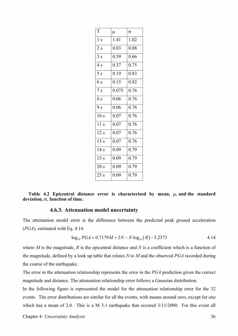
Chapter 4- Uncertainty Analysis 36
T µ σ
1 s 1.41 1.02
2 s 0.83 0.88
3 s 0.59 0.66
4 s 0.37 0.75
5 s 0.19 0.83
6 s 0.15 0.82
7 s 0.075 0.76
8 s 0.06 0.76
9 s 0.06 0.76
10 s 0.07 0.76
11 s 0.07 0.76
12 s 0.07 0.76
13 s 0.07 0.76
14 s 0.09 0.79
15 s 0.09 0.79
20 s 0.09 0.79
25 s 0.09 0.79
Table 4.2 Epicentral distance error is characterized by mean, µ, and the standard deviation, σ, function of time.
4.6.3. Attenuation model uncertainty
The attenuation model error is the difference between the predicted peak ground acceleration
(PGA), estimated with Eq. 4.14.
( )10 10log 0.7179 2 log 3.2373PGA M N N R= + − − 4.14
where M is the magnitude, R is the epicentral distance and N is a coefficient which is a function of
the magnitude, defined by a look up table that relates N to M and the observed PGA recorded during
the course of the earthquake.
The error in the attenuation relationship represents the error in the PGA prediction given the correct
magnitude and distance. The attenuation relationship error follows a Gaussian distribution.
In the following figure is represented the model for the attenuation relationship error for the 32
events. The error distributions are similar for all the events, with means around zero, except for one
which has a mean of 2.0. This is a M 3.1 earthquake that occured 3/11/2000. For this event all

Chapter 4- Uncertainty Analysis 37
stations that recorded detectable ground shaking were with 10 km. The errors in the attenuation
relations are greater at small epicentral distances and in this case predict a higher intensity of
ground shaking than occured. The errors for all events are combined to determine a single Gaussian
error distribution for the attenuation relations. It has a mean of 0.26 and standard deviation equal to
0.9.
Figure 4.8 Attenuation model uncertainty for the 32 events, with thin black line, and the attenuation model error, for all data, with the thick black line. A model for the attenuation relationship error is assumed considering all the events, represented by
a Gaussian distribution with mean as 0.26 and standard deviation equal to 0.9.
4.6.4. Total Error
Error analysis represents a fundamental tool for estimating the error associated to the ground motion
parameter, the single uncertainties are propagated through to the output, that is a function of the
estimated magnitude, M̂ , and the estimated epicentral distance, R̂ :
ˆ ˆ ˆ( , )PGA f M R= 4.15
where f represents ElarmS attenuation relationship Eq. 4.14 (Allen, 2004).
The predicted magnitude and epicentral distance are defined from the true true magnitude M, the
true epicentral distance R, using their time dependent errors εM, εR respectively:
ˆ
ˆ
M
R
M M
R R
ε
ε
= +
= + 4.16

Chapter 4- Uncertainty Analysis 38
The error in the PGA prediction, PGAε , is determined by differencing the logarithm of the observed
and the predicted PGA:
( ) ( ) ( ) ( )ˆlog log log ( , ) logPGA M RPGA PGA f M R PGAε ε ε= − = + + − 4.17
We use the difference in the logarithm of the PGA observation to account for the wide range of
PGA values given the range of magnitudes for the dataset. This is typical in studies of ground
shaking attenuation.
For every observation of magnitude and epicentral distance will be estimated the predicted
magnitude and epicentral distance, M̂ and R̂ , according to Eq. 4.16
The Monte Carlo simulation consists in randomly choosing errors from their distributions to define
the predicted magnitude and location, M̂ and R̂ from Eq. 4.16 and, based on these values the
predicted ground motion parameter, ˆPGA is defined from Eq.4.14.
,ˆ
j i M jM M ε= +
jRij RR ,ˆ ε+=
M1 R1
M2 R2
Mi Ri
Mn Rn
. . . . . . .
. . . . . . ., , ,
ˆ ( ; )i j i M j i R jPGA f M Rε ε= + +
Figure 4.9 Monte Carlo simulation, prediction of ground motion parameter represented by ˆPGA , where for j is indicated the Monte Carlo cycle and for i the observation.
The predicted ˆPGA will be compared with the observed value of PGA and the error will be
evaluated as the difference between prediction and observation, comparing
( ) ( )ˆlog to loge ePGA PGA .
The Monte Carlo simulation procedure is represented in the following figure.
Uncertainty propagation analysis has been carried out for different instants of time from 1 second to
25. For example for instant t we have ( ) ( ) ( )( ), ,tot M R IMt f t tε ε ε ε= that is obtained from Monte
Carlo simulation adopting the error models for andM Rε ε related to instant t . This procedure will
be adopted to build the pdf of the total error related to each 1 sec increment.
The uncertainty associated with the ground motion parameter prediction follows a Gaussian
distribution with mean and standard deviation that vary with time.
The mean goes from a value of –0.61 for 1 second to a value of -0.17 at 5 seconds, finally assuming
a value of 0.16 for 20 seconds.

Chapter 4- Uncertainty Analysis 39
The standard deviation decreases with time going from 1.33 at 1 second to 1.1 at 5 seconds to 1.16
at 20 seconds.
Mi Ri
0 εΜ
p(εΜ)
0 ε R
p (ε R )
M1 R1 PGA1
M2 R2 PGA2
Mi Ri PGAi
Mn Rn PGAn
. . . . . . .
. . . . . . .
,ˆ
i jM ,ˆ
i jR
, , ,ˆ ( ; )i j i M j i R jPGA f M Rε ε= + +
ln ,ˆln( ) ln( )PGA i j iPGA PGAε = −
observation
prediction
Figure 4.10 Monte Carlo simulation: for each observation i , Mi and Ri, and for each cycle j errors, εM and εR, are randomly choosen from their distributions to define the predicted
, ,ˆ ˆ,i j i jM R and then ,
ˆi jPGA to be compared to the observed PGA, in order to define the
distribution of the total error.
The values that characterize the error associated with the PGA prediction are described in the
following table.
t µ σ aad rms
1 s -0.61 1.33 1.15 1.5
5 s -0.17 1.1 0.86 1.1
10 s 0.01 1.02 0.78 1.02
20 s 0.16 0.95 0.73 0.95
25 s 0.16 0.95 0.73 0.95
Table 4.3 The total uncertainty of the prediction is characterized by the mean, µ, the standard deviation, σ, the average absolute deviation, aad, and root mean squared, rms.

Chapter 4- Uncertainty Analysis 40
Figure 4.11 PGA error distribution, result of the uncertainty propagation, as a function of time, where zero time is the instant when the first station is triggered. At this point in order to study the influence of the single error on the total error a sensitivity analysis
has been carried out.
4.6.5. Sensitivity analysis
To determine the largest source of error in the PGA predictions we conduct a simple sensitivity
analysis. The total error in the PGA prediction can be espressed as:
( ) ( )' log ( , ) log ( , )PGA M R Attf M R f M Rε ε ε ε= + + + − 4.18
In order to consider the influence of the single errors, different cases have been considered, the
following table synthesizes the cases.
Case εM εR εATT.M.
1 x x x
2 x x
3 x x
4 x x
Table 4.4The cases considered are defined by different combinations of the errors. We consider four cases (Grasso and Allen, 2005). In case 1 we include all three sources of error in
equation 4.18. The characteristics of 'PGAε are shown in Table 4.9. The errors are of course very
similar to those in Table 4.4 where the total error was determined by differencing the prediction
with the observed PGA. In case 2 we set the error in the magnitude estimate, Mε , to zero thereby

Chapter 4- Uncertainty Analysis 41
assuming an exact magnitude is available for an event and Rε and Attε are the only sources of error
in 'PGAε .
The following cases, from 2 to 4, have been designed in order to isolate and quantify the
contribution of the single errors on the total error.
The Case 1, in which all the error are included, represents the reference point to which compare the
results of the other cases. Comparing the results of the Case 1 obtained with synthetic data to the
results obtained from the error defined as the difference between predictions and real data, is
possible to confirm the perfect aggreement of the results.
In Case 2 the magnitude error influence is evaluated, in the Case 3 the epicentral error is quantified
and finally in Case 4 the attenuation model error influence is weighted.
The results related to Case 2 are synthesized in the following table.
Case 2
t µ σ aad rms
1 s 0.076 0.93 0.74 0.93
5 s 0.18 0.9 0.73 0.92
10 s 0.19 0.9 0.73 0.92
20 s 0.19 0.9 0.73 0.92
25 s 0.19 0.9 0.73 0.92
Table 4.5 The Case 2 is characterized reporting the parameters describing the total error associated with the considered errors, εR and εATT.M.. Analysing the results of Case 2, we can notice that the magnitude error has some influence initially
on the behaviour of the total error of Case 1. The magnitude has negative error, causing a negative
value of the mean in Case 1, that does not happen in Case 2, in which the magnitude error equal to
zero. Considering no magnitude uncertainty is possible to notice that the prediction is still
characterized by an error that has a standard deviation equal to 0.9 for every instant of time
considered, equal to the attenuation model error.
The mean of the error is equal to 0.18 at 5 seconds and 0.19 at 10, 20 and 25 seconds that is equal
to the mean of the attenuation error. These considerations lead to the conclusion that with exact
magnitude value the error is mainly due to the attenuation model error, except for the first second
where location error is of some influence.
Magnitude error has an influence of some importance in the first second, while after 5 seconds the
effect might be neglected.
Case 3, represents the case of correct epicenter location while magnitude and attenuation model are
sources of errors, the results are reported in the following table.

Chapter 4- Uncertainty Analysis 42
Case 3
t µ σ aad rms
1 s -0.48 1.34 1.14 1.43
5 s -0.15 1.125 0.9 1.13
10 s 0.03 1.06 0.8 1.06
20 s 0.2 0.99 0.8 1
25 s 0.2 0.99 0.8 1
Table 4.6 The Case 3 is characterized reporting the parameters describing the total error associated with the considered errors, εΜ and εATT.M.. Observing the results of Case 3 is possible to confirm that the influence of the epicentral distance
error on the total error is present only for the first second, while becomes not influent after 5
seconds. As is possible to notice from the comparison of the results of Case 3 and Case 1 in
correspondance of the first second, the effect of the location error is only on the mean value, while
the other parameters are not influenced.
In the case of location error equal to zero (Case 3), when the magnitude error goes to values close to
zero, the contribution to the prediction error comes only from the attenuation model error, in this
way the error never yields to zero values.
Finally Case 4 is considered in which the attenuation model error is equal to zero.
Case 4
t µ σ aad rms
1 s -0.91 1.03 1.13 1.38
5 s -0.48 0.68 0.67 0.83
10 s -0.3 0.56 0.51 0.64
20 s -0.14 0.43 0.36 0.45
25 s -0.14 0.43 0.36 0.45
Table 4.7 The Case 4 is characterized reporting the parameters describing the total error associated with the considered errors, εΜ and εR. The most important contribution to prediction error is given by the attenaution model error as
confirmed by the results of Case 4.
Is interesting to notice that the mean value goes to a value of –0.14 and the standard deviation
reaches a value of 0.43 less than the values observed in the other cases. The influence of the
attenuation model error is either on mean and on standard deviation for every instant of time
considered.

Chapter 4- Uncertainty Analysis 43
Figure 4.12 Error in PGA as a function of time for the four cases. The mean is shown as a
solid symbol joined by a solid line, plus and minus one standard deviation are shown with open symbols joined by a dashed line. Case 1 (circles) includes all sources of error. Case 2 (squares) neglects error in the magnitude estimate, Mε , but includes epicentral distance error, Rε , and the attenuation relation error, Attε . Case 3 (triangles) neglects Rε but includes
Mε and Attε . Case 4 (stars) neglects Attε but includes Mε and Rε .
Case 1 Case 2 Case 3 Case 4
µ σ aad rms µ σ aad rms µ σ aad rms µ σ aad rms
s -0.66 1.37 1.2 1.52 0.076 0.93 0.74 0.93 -0.48 1.34 1.14 1.43 -0.91 1.03 1.13 1.38
s -0.22 1.12 0.9 1.15 0.18 0.9 0.73 0.92 -0.15 1.125 0.9 1.13 -0.48 0.68 0.67 0.83
0 s -0.04 1.06 0.85 1.06 0.19 0.9 0.73 0.92 0.03 1.06 0.8 1.06 -0.3 0.56 0.51 0.64
5 s 0.12 0.99 0.8 1 0.19 0.9 0.73 0.92 0.2 0.99 0.8 1 -0.14 0.43 0.36 0.45
0 s 0.12 0.99 0.8 1 0.19 0.9 0.73 0.92 0.2 0.99 0.8 1 -0.14 0.43 0.36 0.45
5 s 0.12 0.99 0.8 1 0.19 0.9 0.73 0.92 0.2 0.99 0.8 1 -0.14 0.43 0.36 0.45
Table 4.8 Distribution of errors in the predicted PGA using the ElarmS error model, 'PGAε .
For each case the errors have a Gaussian distribution with mean, µ, the standard deviation, σ. Τhe average absolute deviation, aad, and root mean squared, rms, of the errors are also shown. Case 1 is the total error in PGA which includes errors in the magnitude, Mε , the epicentral distance, Rε , and the attenuation relations, Attε . In Case 2 Mε is set to zero and errors in Rε and Attε only are considered. In Case 3 Rε is set to zero, Mε and Attε only are considered. In Case 4 Attε is set to zero, Mε and Rε only are considered.
In summary, Rε has a negligible contribution to uncertainty in PGA predictions, Mε
contributes initially (the first 5-10 sec only), and Attε is the most significant source of error, particularly at later times after several stations have recoded P-wave arrivals and contribute to the magnitude estimate (Grasso and Allen, 2005).

Chapter 5- Aspects of Feasibility and Reliability of Seismic EWS 44
Chapter 5
5. Aspects of Feasibility and Reliability of Seismic EWS
Main aspetcs involved in feasibility and reliability of an EWS application are:
• the amount of warning time
• the probability of making wrong decisions (false alarms and missed alarms)
that represent, respectively, timeliness and reliability, conflicting requirements of EWS.
These parameters strongly influence EWS impact and effectiveness on seismic risk reduction.
With respect to the first point, the time available to activate security measures is the time interval
from the detection of P-waves in the epicenteral area, and the arrival of S-waves in the area where
the structure or facility is located. This time interval, Tw, defined by Eqs. 2.1 and 2.2, is a function
of the reporting time, Tr, and the S-wave travel time, Ts. The warning time, to be considered
adequate for the activation of a security measure, has to be greater than the time necessary for its
activation.
As a function of the epicentral distance, the area of interest may be decomposed in homogeneous
zones characterized by equal amount of warning time available. This analysis has been carried out
for the San Francisco Bay area (Working Group ‘02) by Allen et al.
Altough for a territorial feasibility assessment for each area has to be evaluated an estimate of
expected annual probability of false alarm and missed alarm in order to have an overview of
possible EWS applications.
Assuming that the warning time provided by the EWS is sufficient for security measure activation,
EWS effectiveness is influenced by system reliability in terms of probability of making wrong
decisions, fundamental aspect in a pre-installation feasibility assessment and for decision making
during the course of the earthquake.
5.1. Probability of wrong decisions in a pre-installation scenario
When examining the feasibility of installing an EWS for a facility, it is important to have a
mechanism to control the probabilities of false and missed alarms. Since the decision to activate the
alarm is based on a predictor, ˆ ,IM false alarms can be caused by the predictor exceeding the
warning threshold even though the actual intensity measure, IM, that occurs at the site does not
reach the critical value. Similarly, missed alarms can be caused by the predictor not exceeding the
warning threshold even though the actual intensity measure reaches its critical value.
For a given facility, the critical threshold, a, of IM may be chosen by the user as the value of IM for
which damage (or high economic losses) is expected to occur with a high probability. However, to

Chapter 5- Aspects of Feasibility and Reliability of Seismic EWS 45
control the probability of wrong decisions, the warning threshold is chosen as the product of the
critical threshold a and a parameter, c, to be specified during the design process. The critical
threshold depends on the facility, structure or equipment to be protected, but the warning threshold
c a⋅ depends on the design process chosen to optimize the warning system. The parameter c
provides a mechanism to control the incidence of false and missed alarms. Note that it is not
possible to simultaneously reduce both but c may be used to control the trade-off between them. A
false alarm occurs when the EWS predicts a value, ˆIM , that exceeds the warning threshold, ac ⋅ ,
while the actual value, IM, of the intensity measure at the site turns out to be less than the value of
the critical threshold, a.
In a pre-installation scenario, the probability of false alarm is therefore given by:
ˆP[ | ]faP IM a IM c a= ≤ > ⋅ 5.1
Similarly the probability of missed alarm is:
ˆP[ | ]maP IM a IM c a= > ≤ ⋅ 5.2
The values of the probabilities of false and missed alarms, Pfa and Pma, are an important tool for the
decision-making process during pre-installation design and during operation in a seismic event.
During design, the anticipated rate of missed and false alarms represents a guideline for
EWS feasibility. The realization of EWS could be feasible or not, depending on whether the
requirements in terms of warning time available and the probability of wrong decisions can be met.
A useful tool to evaluate an EWS may be constructed by using a seismic hazard map to provide the
probability of exceedance of ground shaking intensity, given a site and time interval of interest, to
produce a map of probability of wrong decisions. Such a map would help when performing a
territorial feasibility assessment of EWS applications.
During a seismic event, the (automated) decision to activate protective measures may be done either
by comparing the requirements in terms of warning time needed and the tolerable level of faP
(or maP ) based on the information made available by the EWS, or by monitoring a time-varying
threshold ( )c t a⋅ . This case is examined later in Chapter 7.

Chapter 5- Aspects of Feasibility and Reliability of Seismic EWS 46
5.2. Procedure for estimating Pfa and Pma in a pre-installation scenario
The main reasons for evaluating the probability of wrong decisions in a pre-installation scenario are
to design the warning threshold, following the considerations presented before and, then to define
the probabilities of false and missed alarms and their expected annual frequency that are tolerable to
the owner or manager of the facility to be protected.
The probability of false or missed alarm, in a pre-installation scenario, can be evaluated as a time-
independent variable, based on the seismicity of the area of interest. Time dependence could be
neglected as a first approximation, assuming that the prediction uncertainty stabilizes after a certain
time following the first trigger.
This simplified approach could be applied to special cases as Mexico City where the location of the
fault area, the configuration of the seismic stations enable the possibility of assuming that the
uncertainty of the prediction stabilizes after the first seconds. The time-invariant approach will be
based on the consideration of error as a time independent parameter and we will consider a certain
pdf for the total error related to a certain instant of time.
By estimating the probability of false alarm, before the earthquake, we are primarily trying to
answer to the question: How would an EWS perform during earthquakes that might occur in the
area of interest, in terms of a false (or missed) alarm rate?
Prior information can be expressed by using the hazard (rate) function (Kramer, 1996) that defines
the mean rate per year of events with intensity measure exceeding a certain critical value, given a
site of interest.
The hazard (rate) function provides the information related to the expected intensity measures, IM,
for a given site and period of interest that represents the known parameter in Fig. 5.1; on the other
hand the unknown quantity is represented by the predicted intensity measure, ˆIM , that is evaluated
by adding prediction error, εtot, to the actual IM. The prediction error εtot is defined taking in account
the errors related to the prediction of magnitude, M, epicentral distance, R, and the error of the
ground motion attenuation model. In Fig. 5.1 is represented the relation between the IM and ˆIM
that are related by the εtot, that includes εM, εR and εIM.
The simulated EWS prediction process of ground motion parameters goes backward from the
known intensity measure value, IM, to the predicted value, ˆIM .
The aim is to describe the EWS behaviour for a given seismic event, represented by the
correspondent value of intensity measure, given by the hazard function, and to define the
probability of having false and missed alerts; considering all the possible events, the probability of
wrong decisions is defined, given an area of interest and a period of time of interest (one year), for

Chapter 5- Aspects of Feasibility and Reliability of Seismic EWS 47
all the expected events. The key to forecast the behaviour of the EWS and the predicted value,
given the real value from the hazard function, is the prior knowledge of the errors that we committ
predicting the intensity measure of interest, as a result of the uncertainty propagation of the errors.
The uncertainty propagation, is based on the assumptions of time indepence of the errors of the
earthquake parameters prediction and of the uncertainty related to the attenuation model.
Attenuation Model
M
IM
R
Attenuation Model
M̂
MI ˆ
R̂εR
εM
εIM
εtot
Figure 5.1 Simulation of the EWS process of prediction in a pre-installation analysis.
5.3. Prior information: Hazard function
The hazard (rate) function (Kramer, 1996) gives the mean annual rate of events with intensity
measure exceeding a certain critical value, given a site of interest. From the mean rate, the
probabilty of exceedance of a critical value, given that an earthquake of interest has occurred, can
be defined by considering the rate of exceedance rescaled by the rate corresponding to the minimum
intensity measure of interest (cut-off value), called IM0, assuming a Poisson process for
earthquakes:
0 0( ) ( ) [ | ]c cIM IM P IM IM IM IMλ λ= ⋅ > > 5.3
An exponential model is assumed for the hazard function for a site (but recall that the choice of IM
used in the examples is loge PGA so this corresponds to a power law on PGA):
10( ) 10 k IMIM kλ −= 5.4
where k0 and k1 can be obtained by fitting the hazard function from a PSHA for the site. This model
implies from Eq. 5.3 that (Grasso et al., 2005 a):

Chapter 5- Aspects of Feasibility and Reliability of Seismic EWS 48
[ ] 1 0( )
0| 10 ck IM IMcP IM IM IM IM − −> > = 5.5
The cumulative distribution function is then:
[ ] 1 0( )0| 1 10 ck IM IM
cP IM IM IM IM − −≤ > = − 5.6
and the expression for the PDF (probability density function) is derived by differentiating this
cumulative distribution function:
( ) 1 0 1( )0 1| log 10 10 10k IM IM k IM
ep IM IM IM k c− − −> = ⋅ ⋅ = ⋅ 5.7
where 1 01 log 10 10k IM
ec k= ⋅ ⋅ .
In this work, the parameter k1 is estimated from a hazard function for the site of interest by using a
minimum entropy criterion in which the relative entropy E is minimized with respect to k1:
log ii
i i
pE pq
⎛ ⎞= ⎜ ⎟
⎝ ⎠∑ 5.8
where pi represents the discrete probability distribution function derived from ( )0|p IM IM IM>
and qi is the discrete probability distribution function derived from the given hazard function
( )IMλ using Eq. 12, so qi is obtained by numerically differentiating the cumulative distribution
function in the same way as ( )0|p IM IM IM> was derived above. Therefore, pi is a function of
the parameter k1 but qi is not. By minimizing the relative entropy, we determine the parameter k1 so
that the model PDF is the best fit in an information-theoretic sense to the PDF implied by the
hazard function for the site.
5.4. Probability of false alarm in a pre-installation scenario
The probability of false alarm, as defined in Eq.5.1, for Bayes rule can be expressed as:
0
0
0
ˆ| ,
ˆ |
ˆ |
faP P IM a IM c a IM IM
P IM a IM c a IM IM
P IM c a IM IM
⎡ ⎤= ≤ > ⋅ >⎣ ⎦⎡ ⎤≤ ∩ > ⋅ >⎣ ⎦=
⎡ ⎤> ⋅ >⎣ ⎦
5.9

Chapter 5- Aspects of Feasibility and Reliability of Seismic EWS 49
where it is assumed that an earthquake of interest, i.e. 0IM IM> , has occurred and that 0a IM> .
The numerator, let us call it Pfa,1, is evaluated as:
0
,1 0
0
ˆ |
ˆ ˆ ( , | )
fa
a
ca IM
P P IM a IM c a IM IM
p IM IM IM IM dIMdIM∞
⎡ ⎤= ≤ ∩ > ⋅ >⎣ ⎦
= >∫ ∫ 5.10
which can be written, using Bayes rule, as:
0
,1 0ˆ ˆ( | ) ( | )
a
faIM ca
P p IM IM p IM IM IM dIMdIM∞
= ⋅ >∫ ∫ 5.11
where ( )0|p IM IM IM> is given by Eq. 5.7 and )|ˆ( IMMIp is a Gaussian distribution with IM
representing the mean value (if εtot has zero mean) and standard deviation σtot given by uncertainty
propagation (Chapter 4). In the case that the prediction, ˆ ,IM is affected by a significant bias error
(i.e. mean µtot of εtot is not close to zero), then the mean of the Gaussian distribution )|ˆ( IMMIp is
(IM ± µtot) (from the dfinition of the prediction error as difference between prediction and
observation). Substituting in Eq. 5.11:
1
0
,1
2ˆ1
21 ˆexp 10
2
ak IM
faIM ca tot
IM IMtot
P c dIMdIMσσ π
∞⎛ ⎞ −⎜ ⎟⎜ ⎟⎝ ⎠
−−⎡ ⎤
= ⋅ ⋅⎢ ⎥⎣ ⎦
∫ ∫ 5.12
The integral of the Gaussian distribution over ˆIM can be expressed in terms of the standard
Gaussian cumulative distribution function Φ:
2
ˆ12
1 ˆexp2ca tot
ca IMIM IMtot tot
dIMσ σσ π
∞⎛ ⎞⎜ ⎟⎜ ⎟⎝ ⎠
−−− −⎡ ⎤ ⎛ ⎞
= Φ⎢ ⎥ ⎜ ⎟⎝ ⎠⎣ ⎦
∫ 5.13
so Eq. 5.11 can be cast in a simpler form:
1
0
,1 10a
k IMfa
IM
ca IM
totP c dIM
σ
−−−
⎛ ⎞= Φ ⋅ ⋅⎜ ⎟
⎝ ⎠∫ 5.14

Chapter 5- Aspects of Feasibility and Reliability of Seismic EWS 50
The denominator of Pfa in Eq. 5.9 is expressed as:
,2 0ˆ ˆ( | )fa
ca
P p IM IM IM dIM∞
= >∫ 5.15
which can be written, using the theorem of total probability, as:
0
,2 0ˆ ˆ( | ) ( | )fa
IM ca
P p IM IM p IM IM IM dIMdIM∞ ∞
= ⋅ >∫ ∫ 5.16
This can be expressed in terms of the standard Gaussian cumulative distribution function Φ as:
1
0
,2 10 k IMfa
IM
ca IM
totP c dIM
σ
∞−−
−⎛ ⎞
= Φ ⋅ ⋅⎜ ⎟⎝ ⎠
∫ 5.17
Summarizing, the probability of false alarm in a pre-installation analysis is given by (Grasso et al. 2005 a):
1
0
1
0
10
10
ak IM
IMfa
k IM
IM
ca IM
tot
ca IM
tot
dIMP
dIM
σ
σ
−
∞−
−−
−−
⎛ ⎞Φ ⋅⎜ ⎟
⎝ ⎠=⎛ ⎞
Φ ⋅⎜ ⎟⎝ ⎠
∫
∫ 5.18
The integrals in the denominator and numerator here can be evaluated numerically for different
values of c, given the value of a; then curves of Pfa versus c can be plotted for different critical
thresholds a. Examples are given later in Chapter 6.
5.5. Probability of missed alarm in a pre-installation scenario
The probability of missed alarms, as defined in Eq.5.2, can be written using Bayes rule as:

Chapter 5- Aspects of Feasibility and Reliability of Seismic EWS 51
0
0
0
ˆ| ,
ˆ |ˆ |
maP P IM a IM c a IM IM
P IM a IM c a IM IM
P IM c a IM IM
⎡ ⎤= > ≤ ⋅ >⎣ ⎦⎡ ⎤> ∩ ≤ ⋅ >⎣ ⎦=
⎡ ⎤≤ ⋅ >⎣ ⎦
5.19
where once again it is assumed that an earthquake of interest has occurred and that 0a IM> . The
numerator can be expressed as:
,1 0
0
ˆ |
ˆ ˆ ( , | )
ma
ca
a
P P IM a IM c a IM IM
p IM IM IM IM dIMdIM∞
−∞
⎡ ⎤= > ∩ ≤ ⋅ >⎣ ⎦
= >∫ ∫ 5.20
which can be written, using Bayes rule, as:
,1 0ˆ ˆ( | ) ( | )
ca
maa
P p IM IM p IM IM IM dIMdIM∞
−∞
= ⋅ >∫ ∫ 5.21
where ( )0|p IM IM IM> is given by Eq. 5.7 and )|ˆ( IMMIp is a Gaussian distribution as before
(see after Eq. 5.11). Substituting in Eq. 5.21:
1,1
2ˆ1
21 ˆexp 10
2
cak IM
maa tot
IM IMtot
P c dIMdIMσσ π
∞⎛ ⎞ −⎜ ⎟⎜ ⎟⎝ ⎠−∞
−−⎡ ⎤
= ⋅ ⋅⎢ ⎥⎣ ⎦
∫ ∫ 5.22
The integral of the Gaussian distribution over MI ˆ can be expressed in terms of the standard
Gaussian cumulative distribution function Φ:
2
ˆ12
1 ˆexp 2
ca
tot
ca IMIM IMtot tot
dIMσ σσ π⎛ ⎞⎜ ⎟⎜ ⎟⎝ ⎠−∞
−−−⎡ ⎤ ⎛ ⎞
= Φ⎢ ⎥ ⎜ ⎟⎝ ⎠⎣ ⎦
∫ 5.23
so Eq. 5.22 can be cast in a simpler form:
1,1 10 k IM
maa
ca IM
totP c dIM
σ
∞−−⎛ ⎞
= Φ ⋅ ⋅⎜ ⎟⎝ ⎠
∫ 5.24
The denominator of Pma in Eq. 5.19 is:

Chapter 5- Aspects of Feasibility and Reliability of Seismic EWS 52
,2 0ˆ ˆ( | )
ca
maP p IM IM IM dIM−∞
= >∫ 5.25
which can be expressed, using the theorem of total probability, as:
0
,2 0ˆ ˆ( | ) ( | )
ca
maIM
P p IM IM p IM IM IM dIMdIM∞
−∞
= ⋅ >∫ ∫ 5.26
This can be expressed in terms of the standard Gaussian cumulative distribution function:
1
0
,2 10 k IMma
IM
ca IM
totP c dIM
σ
∞−−⎛ ⎞
= Φ ⋅ ⋅⎜ ⎟⎝ ⎠
∫ 5.27
The probability of missed alarms in a pre-installation analysis is therefore given by (Grasso et al.
2005 a):
1
1
0
10
10
k IM
ama
k IM
IM
ca IM
tot
ca IM
tot
dIMP
dIM
σ
σ
∞−
∞−
−
−
⎛ ⎞Φ ⋅⎜ ⎟
⎝ ⎠=⎛ ⎞
Φ ⋅⎜ ⎟⎝ ⎠
∫
∫ 5.28

Charter 6- Warning threshold design and Feasibility assessment 53
Chapter 6
6. Warning threshold design and Feasibility assessment
6.1. Designing the test procedure: warning threshold setting
The warning threshold is the EWS parameter that most influences the onsequences impact of a
decision this is the reason why accuracy and attention is needed for threshold design procedure.
Two performance-based methods are described for warning threshold design. The first method is
based on the operating characteristic (OC) function and the second one on cost-benefit
considerations.
A test procedure leading to the acceptance\rejection of a hypothesis is simply a rule specifying
whenever the hypothesis should be accepted or rejected based on the observed data. In our case
accepting/rejecting the hypothesis means raising the alarm or doing nothing.
Designing a test procedure, can be defined by subdividing the sample space of all possible values
that the predictor can assume, in two exclusive regions (Wald, 1947).
The space of all the possible samples is divided in:
• Region 1, for which acceptance of the hypothesis is prefered
• Region 2, is the critical region, for which rejection of the hypothesis is prefered
Considering the hypothesis of threshold exceedance, the critical region (2) is represented by all the
values of intensity measure for which the alarm has to be activated and region 1 where the alarm
has not to be activated.
The critical region is defined by the critical threshold, that is a given design parameter, provided by
the user, representing the occurrence of structural damage or heavy economic losses.
The warning threshold corresponds to raising the alarm.
The warning threshold is defined by a decision criteria, based on user’s requirements, that could be
based on tolerable level of probability of wrong decion or on cost-benefit considerations.
The process of warning threshold design is described for both the situations, in which the
constraints are related to tolerable level of wrong decision rate, in the first case, and to cost-benefit
analysis, in the other case.
The test is designed defining the critical regions, by assignig the alarm threshold ca that satisfyies
the user’s requirements.

Charter 6- Warning threshold design and Feasibility assessment 54
6.2. Threshold setting based on OC function
In the case that the user’s requirements are given as the tolerable values of probabilities of false and
missed alarms, the test procedure can be designed as follows.
The goal is to design a test that satisfies the conditions imposed on Pfa (or Pma) by controlling the
alarm threshold c·a on ˆIM . If the probability of false alarms is lowered, then the probability of
missed alarms is increased. To design the alarm threshold for IM, the trade-off between Pfa and Pma
must be studied. Because of this trade-off, there is a limit as to how much the probabilities of wrong
decisions can be reduced. This limit can be studied by using Stein’s lemma, which states:
If a large number N of observations is available, then as Pma → 0, [ ]0 1exp ( , )faP N K p p→ −
where K is the relative entropy (Kullback-Leibler distance):
10 1 1
0
( , ) logepK p p p dIMp
= ∫ 6.1
where p0 is the PDF of IM conditioned on ˆIM c a≤ ⋅ (null hypothesis) and p1 is the PDF of IM
conditioned on ˆIM c a> ⋅ .
Based on the user’s specifications of tolerable Pma, the corresponding Pfa is given by Stein’s
Lemma. By means of the operating characteristic (OC) function, the warning threshold can be
defined. The OC function represents the probability of acceptance of the null hypothesis which
corresponds to the probability of no alarm activation.
The ideal test corresponds to the ideal OC function shown in Figure 6.1, which gives a probability
of acceptance of 1 for IM a≤ when ˆIM c a≤ ⋅ (in acceptance zone) and probability of acceptance
of zero for IM a≤ when ˆIM c a> ⋅ (in the rejection zone). Note that the probability of acceptance
conditioned on the predictor, ˆIM , may be written as ˆ|P IM a IM⎡ ⎤≤⎣ ⎦ , that corresponds to Pfa in the
rejection (critical) zone and (1- Pma) in the acceptance zone.

Charter 6- Warning threshold design and Feasibility assessment 55
ca MI ˆ
1
ˆ|P IM a IM⎡ ⎤≤⎣ ⎦
Figure 6.1 The ideal OC function
Based on uncertainties in the prediction of IM by ˆIM , which is based on the first seconds of
observation of the seismic data, we cannot obtain an ideal OC function and we have to accept errors
of type I and II (missed and false alarms). If the tolerable probability of a missed alarm in the
acceptance zone is α and the tolerable probability of false alarm is β in the rejection zone, then the
OC function will be characterized as in Figure 6.2 where β (or α) is the design requirement
specified by the user and α (or β), respectively, is given by Stein’s Lemma. The test is better
designed if the OC function corresponding to the test is closer to the optimal OC function
represented in Figure 5.
A prior definition of a possible set of thresholds, c a⋅ , can be defined and for each value of a the
optimal OC function is defined. The discrete OC function representing the test may be evaluated at
a finite number of points representative of the values of probabilities of wrong decisions for a range
of values of c a⋅ of interest. A best fitting curve can be constructed based on these points and the
corresponding value of c a⋅ will be the optimal warning threshold.
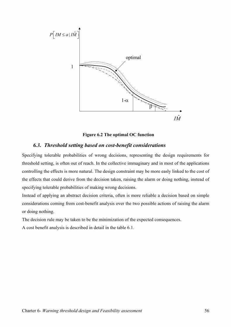
Charter 6- Warning threshold design and Feasibility assessment 56
MI ˆ
1
1-αβ
optimal
ˆ|P IM a IM⎡ ⎤≤⎣ ⎦
Figure 6.2 The optimal OC function
6.3. Threshold setting based on cost-benefit considerations
Specifying tolerable probabilities of wrong decisions, representing the design requirements for
threshold setting, is often out of reach. In the collective immaginary and in most of the applications
controlling the effects is more natural. The design constraint may be more easly linked to the cost of
the effects that could derive from the decision taken, raising the alarm or doing nothing, instead of
specifying tolerable probabilities of making wrong decisions.
Instead of applying an abstract decision criteria, often is more reliable a decision based on simple
considerations coming from cost-benefit analysis over the two possible actions of raising the alarm
or doing nothing.
The decision rule may be taken to be the minimization of the expected consequences.
A cost benefit analysis is described in detail in the table 6.1.

Charter 6- Warning threshold design and Feasibility assessment 57
Action Case: IM<a Case: IM>a
Raise Alarm False alarm:
Cfa
Good Alarm:
Cga
No Alarm Good Missed Alarm:
Cgm
Missed Alarm:
Cma
Table 6.1 Cost benefit analysis for threshold design
Where:
0
1
1
ga eq save
ma eq
gm
ga fa
gm ma
C C C
C C
C
P P
P P
= −
=
= −
= −
6.2
Where Ceq represents the expected costs due to the earthquake, Csave the expected savings as a
consequence of the security measure activation, Cfa is the cost of a false alarm and Cma is the cost of
a missed alarm.
In the case we decide to raise the alarm, the expected cost is represented by:
[ ]
( ) ( )cos |
1fa fa ga ga
fa fa eq save fa
E t alarm C P C P
C P C C P
= ⋅ + ⋅
= ⋅ + − ⋅ − 6.3
In the case we decide not to raise the alarm, the expected cost is defined by:
[ ]cos | gm gm ma ma
ma ma
E t no alarm C P C P
C P
− = ⋅ + ⋅
= ⋅ 6.4
The decision criteria for deciding between the options, raising the alarm or not, is represented by the
minimum cost rule:
Raise the alarm if and only if:
[ ] [ ]cos | cos |E t no alarm E t alarm− ≥ 6.5

Charter 6- Warning threshold design and Feasibility assessment 58
( ) (1 )
( ) ( )eq ma fa fa eq save fa
save fa eq fa eq save
C P C P C C P
C C C P C C
⋅ ≥ ⋅ + − ⋅ −
= + − ⋅ + − 6.6
Eq. 6.6 can be taken as an equality used to select an appropriate value of c, solving the equation for
Pfa (or Pma). The tolerable value of Pma (Pfa) may then be determined from Eq. 5.33 (or Eq. 5.21) for
this value of c.
The tolerable value of Pfa (or Pma) may be used for:
− evaluate the warning threshold, when the time-invariant approach is applicable
− alarm activation during the event while monitoring the Pfa (or Pma), when the time invariant
approach is not applicable
In order to evaluate the warning threshold assuming that the time invariant approach is applicable,
(σtot in Eq. 5.18 and 5.28 is time invariant) the first step is to calculate the Pfa (or Pma) given by Eq.
5.21 and 5.33 for a range of interest of values of warning threshold, given the value of critical
threshold, a, that is a design data given from the user.
Then defined a curve that represents the Pfa (or Pma) as a function of c a⋅ we can evaluate the value
of c a⋅ that corresponds to Pfa (or Pma) equal to the tolerable level β (α) evaluated in Eq. 6.6.
During a seismic event, however, more and more information becomes available to the EWS and so
σtot will decrease with time. A refined analysis using a time-dependent warning threshold, c(t)a,
would then be more appropriate. Alternatively, the probability of false and missed alarms could be
monitored as a function of time and then the alarm would be raised when the tolerable level of
probability of Pfa(t) or Pma(t) is exceeded.
In the next chapter, we consider a refined decision-making procedure that is appropriate during a
seismic event and which takes into account that the quality of the IM prediction improves as more
and more information is obtained by the EWS. It is shown in Chapter 7 that in this case: Pfa(t) +
Pma(t) =1, so Eq. 6.6 implies that the probability of a false alarm is tolerable if and only if:
( ) savefa
fa save
CP tC C
β≤ =+
6.7
Similarly, since the alarm is not raised if and only if:
( ) ( )eq ma save fa eq fa eq saveC P C C C P C C⋅ < + − ⋅ + − 6.8
it follows that the probability of a missed alarm is tolerable if and only if:

Charter 6- Warning threshold design and Feasibility assessment 59
( ) fama
fa save
CP t
C Cα< =
+ 6.9
It is clear from Eq. 6.7 and 6.9 that in this case, where the decision criterion is based on a cost-
benefit analysis, 1α β+ = , which directly exhibits the trade-off between the threshold probabilities
that are tolerable for false and missed alarms. If the threshold β is reduced to make false alarms less
likely, then the threshold α for missed alarms becomes correspondingly larger.
6.4. Threshold design and Feasibility assessment: an example for Southern
California
In the hypothesis of a future realization of an EWS for the protection of Southern California, in this
section will be addressed a feasibility assessment of the application of interest of the potential end-
user of the EWS (Grasso et al. 2005 a).
In particular we will be answering to the question: How would an EWS perform during earthquakes
that might occurr in the area of interest, in terms of false and missed alarm rate?
We might quantify the effectiveness of the EWS application, by providing to the end-user of the
EWS the probabilities of wrong decisions to see whether they are acceptable or not and on the other
hand we will be able to set the warning threshold in order to match the user’s requirements.
In case of existing EWS application we might be interested in assessing the reliability of the system
in terms of probabilities of making wrong decisions. The values of critical and warning thershold
for an existing application are known parameters. For the given facility we can build the curves
representing Pfa and Pma as a function of the warning threshold ca (Eq. 5.18 and 5.28). We will be
able to define the probabilities of wrong decisions related to the critical threshold and warning
threshold that define the existing application. We could discover that the tolerable levels of
incidence of false or missed alarms are not met. Based on the tolerable level of probability of wrong
decisions we will be able to adjust the warning threshold, if time-invariant approach is applicable.
Assuming to be interested in Southern California, based on the Hazard function provided for the
area of Los Angeles, we will evaluate the probabilities of wrong decision as a function of the
warning coeffient, c. Assuming to know the critical threshold, a, provided by the user, the warning
threshold will be set based on the design requirements in case of new EWS application (if time-
invariant approach is applicable).
In case of existing application, given the value of the critical threshold, a, and the warning
threshold, ca, the performance and feasibility assessment of the EWS application will be carried out
by evaluating the corresponding expected annual probabilities of wrong decisions (Eq. 5.18 and

Charter 6- Warning threshold design and Feasibility assessment 60
5.28). If the annual probabilities of wrong decision result not acceptable the warning threshold will
be set in order to match the tolerable levels ( assuming that the time-invariant approach is
applicable).
Cua and Heaton prediction method is choosen as the earthquake predictive model (M1 in the
Fig.4.3) of interest, the attenuation model used (M2 in Fig.4.3) is the Cua and Heaton relation and
the intensity measure parameter of interest provided in output is the peak ground acceleration in
log10 scale (Eq. 2.11).
The parameters a, b, d, e, in Eq. 2.11 are defined by Cua and Heaton (2004) for different soil types.
Rock type has been considered, where: 30.779; 2.55 10 ;a b −= = ⋅ 1.352; 0.645; (0,0.243)d e Gaussianε= = − = .
The intensity measure IM is the peak ground acceleration (PGA) on a log10 scale. The chosen
hazard function for the Los Angeles area is shown in the following figure and it represents the mean
rate of exceedance versus PGA in g units. The hazard function is fitted, as described previously, by
using a minimum relative entropy criterion in order to define the coefficient k1 to describe the
probability distribution function of IM. Minimizing the relative entropy, a value of k1=1.06 is
obtained.
0
0.5
1
1.5
2
2.5
3
3.5
4
4.5
0 0.5 1 1.5 2 2.5
PGA(g)
λ(PGAc)
Figure 6.3 Hazard function for Los Angeles representing the annual probability of
exceedance of PGA.

Charter 6- Warning threshold design and Feasibility assessment 61
0
0.1
0.2
0.3
0.4
0.5
0.6
0.7
0.8
0.9
0 0.5 1 1.5 2 2.5 3 3.5PGA (g)
λ(PGAc) Data
Power-Law
k1=1.06
Figure 6.4 Fitting the Hazard function for Los Angeles with power-law
In order to simulate the behaviour of the EWS, in the prediction process we need to know the total
error associated to the process, defined in the uncertainty propagation analysis.
In uncertainty propagation based on the assumption of time independency of the errors, will be
chosen:
• εM : Gaussian (0, 0.5)
• εR : ignored at this stage
• εIM : Gaussian (0, 0.243)
correspondent to the error pdf of magnitude at 4 sec (Cua and Heaton, 2004) and for the attenuation
model error, respectively, neglecting at this stage the epicentral distance error.
The total error associated to the predicted ˆIM , is defined as described in Chapter 4 (uncertainty
propagation):
• εtot : Gaussian (0, 0.44)
Modeling the total error associated with the predicition is fundamental step for evaluating the
consequences of a making wrong decison.
The probabilities of false and missed alarm are evaluated based on the Eq.5.18 and 5.28 as a
function of the warning threshold factor, c, for different values of the critical threshold, a. Notice
that for Pfa in the approximate range of 0.05 to 0.4, the choice of c is insensitive to a.

Charter 6- Warning threshold design and Feasibility assessment 62
0
0.1
0.2
0.3
0.4
0.5
0.6
0.7
0.8
0.9
1
0 0.5 1 1.5 2 2.5 3 3.5c
Pfa
a=0.03 g
a=0.025 g
a=0.1 g
a=0.05 g
Figure 6.5 Probability of false alarm as a function of warning threshold factor c for
different critical thresholds, a, expressed in g’s.
0
0.05
0.1
0.15
0.2
0.25
0.3
0.35
0.4
0.45
0.5
0 0.5 1 1.5 2 2.5 3 3.5c
Pma
a=0.1 g
a=0.03 g
a=0.025 g
a=0.05 g
Figure 6.6 Probability of missed alarm as a function of warning threshold factor c for
different critical thresholds, a, expressed in g’s. if it is false alarms that the the user is most concerned about, the warning threshold will be set so
that the tolerable level of false alarm will not be exceeded.
If the tolerable level of probability of false alarm is equal to 0.4, given the critical threshold equal to
2 cm/s/s, the warning thereshold will be set equal to 2.22 (Fig. 6.7).

Charter 6- Warning threshold design and Feasibility assessment 63
From Fig. 6.8 assuming the warning threshold equal to 2.22 and given the critical threshold equal to
2 cm/s/s, we will obtain a Pma of 0.045, that has to be accepted .
If this value of Pma is not acceptable (tolerable level is exceeded) the warning threhold value has to
be redesigned iteratively till the requirements are matched.
The graphs of Pfa (or Pma) vs. the warning threshold factor, c, are useful, in the case of existing
application, for performance and feasibility assessment of the EWS application. For example in the
case of 2 / /a ca cm s s= = the corresponding Pfa is 0.8 and Pma is 0.025 (from Fig. 6.7 and 6.8).
assuming that the user is concerned on false alerts and from the cost-benefit analysi comes out that
the tolerable level of Pfa is equal to 0.4, the threshold settings result inadequate. Is important to point
out that Pfa and Pma are parameters that can be controlled.
We will use again the graphs in Fig. 6.7 and 6.8 assuming 0.4faP β= = . Based on this requirement
we will be able to redesign the warning threshold in order to match the requirements, assuming
time-invariant approach is applicable.
The warning threshold corresponding to the condition 0.4faP β= = is equal to 2.2 cm/s/s. Due to
the trade-off between false and missed alerts the Pma value increased from a value of 0.025 to a
value of 0.42. Can we accept this value of Pma? If the answer is positive the process ends accepting
the “new” warning threshold. If not we have to iterate the process several times until the conditions
on Pfa and Pma are met. Fig. 6.9 visualizes the trade-off between Pfa and Pma..
0
0.1
0.2
0.3
0.4
0.5
0.6
0.7
0.8
0.9
1
0 1 2 3 4 5 6ca
Pfa a=a'
β
Figure 6.7 The curve represents the probability of false alarm for a given critical
threshold a’ equal to 2 cm/s/s, as a function of the warning threshold. Defined the tolerable value of probabilità of false alarm, as described above, is possibile to define the correspondent warning threshold.

Charter 6- Warning threshold design and Feasibility assessment 64
0
0.02
0.04
0.06
0.08
0.1
0.12
0 1 2 3 4 5 6ca
Pma a=a'
Figure 6.8 The curve represents the probability of missed alarm for a given critical
threshold a’ equal to 2 cm/s/s, as a function of the warning threshold. Defined the tolerable value of warning threshold as described above, is possibile to define the correspondent probability of missed alarm to be accepted.
0
0.1
0.2
0.3
0.4
0.5
0.6
0.7
0.8
0.9
1
0 1 2 3 4 5 6ca
Pma
a=a'Pfa
Figure 6.9 The curve represent the probability of false (blue line) and missed alarm (red line) as a function of the warning threshold. This graph visualizes the trade-off between probability of false and missed alarm, decreasing the tolerable level of probability of false alarm we will have as a consequence an increase of probability of missed alarm that we will have to accept. On the other hand the curves represented in Fig. 6.5 and 6.6 will give a sense of the feasible
applications representing the probabilities of false and missed alarm for a given area of interest. In
this way is possible to map and decompose the areas surrounding the epicentral one in
homogeneous areas that will be characterized by a certain amount of warning time and an expected

Charter 6- Warning threshold design and Feasibility assessment 65
probability of wrong decision. Based on this information for each area of interest it will be possible
to assess the feasible EWS applications.

Chapter 7- Operational Aspects of EWS: Decision Making 66
Chapter 7
7. Operational aspects of EWS: Decision making
7.1. Sequential test
During the seismic event we have to decide between the two options: raise the alarm, do nothing.
This decision is based on a parameter, the so called predictor. The decision problem may be
approached by the theory of hypothesis testing (Wald 1947) . The sequential method of testing an
hypothesis may be described as follows. A rule is given for making one of the following three
decisions during the course of the seismic event:
• Accept the hypothesis
• Reject the hypothesis
• Continue and make an additional observation.
Such a test is carried out sequentially. On the basis of the first observation a decision is made. In the
case the first option is choosen (accept) the process is ended, if the second or third decision (reject
or continue) is made a second observation is made. Again on the basis of the first two observations
a decision is made. If the second or third decision is made a third trial is made and so on. The
process is carried out till one of the first decisions is made. The number of observations is a random
number depending on the outcome of the observations.
In our case the decision is made based on the observation of the predictor that represents the
outcome of the prediction process of the EWS. A rule for making one of the three decisions consists
in defining the critical region. For each observation the hypothesis will be accepted or rejected if the
observation lies in the critical region or not. At every trial the observation will be drawn and
compared with the critical region. Lets consider an example of sequential test. The case is of a lot of
manifactured products that has to be accepted or rejected depending on the outcome of the
inspection. Each product may be considered defective or non-defective and the lot will be accepted
if the probability of defectives in the lot is less or equal than a given value p’, that corresponds to a
number no of defectives. The lot will be rejected if the portion of defectives is greater than this
value. In this case the hypothesis that we are testing is that 'p p≤ . Given the value of no, if the first
no units inspected will be non-defective, the lot will be accepted. If in the first om n≤ there is a unit
that is defective, the lot will be rejected. The critical region is the key aspect of a sequential test.
The principles of a proper choice of the critical region are based on the study of the consequences of
any decision.
The critical region has been defined in the previous sections in the case the tolerable level of wrong

Chapter 7- Operational Aspects of EWS: Decision Making 67
decision is known or based on cost-benefit considerations. Given the critical region we might want
to investigate the degree of acceptance and rejection of the null hypothesis.
In the case there is only one unknown parameter φ in the process (i.e. the value of the predictor) the
null hypothesis consists in oφ φ≤ . The hypothesis will be accepted if the parameter is less or equal
than the critical one and rejected if is greater. Lets now analyse the degree for acceptance and
rejection. For example the rejection of the hypothesis is not considered a serious error if oφ φ≤ but
near the boundary. Similarly the acceptance of the hypothesis will not be a serious error if the
parameter is greater than the critical value but near the boundary of the critical area. If the point is
right on the boundary the hypothesis may be accepted or rejected. The parameter space may be
subdivided in three areas, the first one in which the acceptance is strongly preferred, the second one
in which the rejection is strongly preferred and the last one in which there is no preference of
acceptance or rejection. The subdivision of the space in the three areas gives an idea of the degree
of preference for acceptance or rejection that will be better described by two functions of the
parameter φ : fο that expresses the importance of the consequence of accepting the hypothesis when
we should have not and f1 the importance of rejecting the hypothesis when we should have not. For
example in the zone of preference for rejection fο has a high positive value that represents the cost
of acceptance, in this situation the f1 will have a loss that will be very low. The dependence of
preference for one action or another is related to the subdivision of the area of the samples in three
areas, quantified by the functions fο and f1.
The functions fο and f1 represent a guideline for decision making representing the degree of
preference of one action or the other. The process consists not only in observing the parameter of
interest but monitoring the functions fο and f1. Τhese functions represent the consequences of taking
action, i.e. false and missed alarm, loss caused by making a wrong decisions, etc.
In the following sections the decision process will be explained, based on sequential testing, during
a seismic event, by monitoring the predictor and the functions representing the consequences of
taking action.
The analysis has been first approached by choosing the probability of false and missed alarm as
coincident to the fο and f1 and then the analysis has been extended to the observation of other
consequences as economic loss, structural damage etc (Chapter 8).
7.2. Operational aspects of EWS
During a seismic event, the probability of false and missed alarms will be updated with time as
more stations are triggered by the seismic waves and more data comes in from those that have
already been triggered. This increase in data available will produce a decrease with time in the

Chapter 7- Operational Aspects of EWS: Decision Making 68
uncertainty in the predicted earthquake location and magnitude. Therefore, the prediction of the
intensity measure can be updated with time and the characterization of its uncertainty, εtot (t), will
vary with time. As a consequence, it is important to update the probability of false and missed
alarms as the seismic event evolves.
The necessity of a time-dependent method for the evaluation of the probability of false becomes
essential. As more stations are triggered, the predictions (magnitude and epicentral distance) will be
updated and their uncertainty as well, as a consequence the prediction of the intensity measure will
be updated with time and its uncertainty, εtot (t), function of time.
The IM that will be observed is unknown, the higher is the quality of the prediction the closer the
value of the observed intensity measure will be to the prediction, that is a known parameter at each
instant of time, when the predictions of magnitude and location and their uncertainties are available.
Attenuation Model
M
IM
R
Attenuation Model
M̂
MI ˆ
R̂εR(t)
εM(t)
εIM
εtot(t)
Figure 7.1 Simulation of the EWS prediction process, during the seismic event. In a real-time analysis, during the seismic event, the information that results known is the prediction
provided by the EWS prediction process, while in a off-line analysis the known parameter is the
observation.
Given the prediction the value of the predictor that will be observed will be a value close or not to
the prediction depending on the accuracy of the prediction process, represented by total error
defined by the error analysis in the previous chapters.
The IM that will be observed may be assumed as a random variable of Gaussian distribution with
mean equal to the prediction MI ˆ and pdf given by the Bayesian approach (Virtual Seismologist
Method, Cua and Heaton 2004) or by uncertainty propagation of the error.
The more the prediction process is accurate the more the distribution is peaked around the
prediction. The assumption of IM normally distributed around the prediction is confirmed by the
error analysis for ElarmS performance assessment, where from the results of the error analysis the
Chapter 7- Operational Aspects of EWS: Decision Making 69
total error resulted well modeled by a Gaussain distribution.
In the real-time analysis the values of predicted magnitude, epicentral distance, provided by the
EWS, will be used to estimate the predicted intensity measure MI ˆ , by the means of the attenuation
model.
( ) ( ) ( )ˆtotIM t IM t tε= + 7.1
Fundametal informations to be provided are the uncertainties of the predictions of M, R, εM, εR that
as more data become available will be updated with time and will be ued to define the total error
related to the prediction, εtot (t), characterized by a Gaussian distribution with zero mean and
standard deviation given by uncertainty analysis (Chapter 4).
The total error represents the quality of the information provided by the EWS and is a basic
information for consequences evaluation, representing the main source of wrong decisions.
7.3. Probability of wrong decisions in a real-time analysis
In this section we examine the decision-rule criterion chosen for decision making during the seismic
event, that will represent the guideline to decide between raising the alarm and doing nothing.
The decision between an action or the other will be guided by the observation of the predictor and
the degree of preference between the options.
The degree of preference may be considered as a measurable parameter. Degree of preference is
considered to be connected to the concept of utility (Von Neumann and Morgenstern, 1945).
A numerical approach to utility is dependent on the possibility of comparing differences in utility.
As an example for giving the sense of the measurable characteristic of utility as degree of
preference of an event may be given by the very natural attitude of individuals to have a clear
intuition of preferences of two objects or events. For any two alternatives the individual will
associate probabilities. Associating a probability to an event or a combination of events he will
intuitively prefer the one to the other. At same way the use of probabilities of errors will guide the
user and define a rule for quantifying the preference for the possible actions, in our case raising the
alarm or doing nothing.
A decision rule may be based on the probability of error criterion (Melsa and Cohn, 1978) related to
the analysis of the probabilities of error. In our case the possible errors of interest are, as defined
before, false and missed alarm. The total probability of error is defined as:
e eI eIIP P P= + 7.2

Chapter 7- Operational Aspects of EWS: Decision Making 70
being the two conditions mutually exclusive.
The probabilities andeI eIIP P represent respectively the probability of a missed and of a false alert.
During the seismic event andeI eIIP P represent potential probabilities of wrong decision that will
become probabilities of wrong decision when a decision is made.
In particular, the (potential) probability of false alarm is estimated as the probability of IM being
less than the critical threshold, a, (if the alarm is raised becomes an probability of false alarm):
ˆ( ) P[ | ]faP t IM a IM= ≤ 7.3
Considering that the IM has a normal distribution with mean equal to the predicted MI ˆ (if there is a
known bias in the prediction totµ it should be added to this mean) and standard deviation totσ
evaluated as a function of the updated uncertainties (uncertainty propagation methods, Chapter 4):
( ) ( )
2ˆ( ( ))22
ˆ1 - ( )( ) exp( )2
a
fatottot
IM IM tttot
a IM tP t dIMtt σ σσ π−∞
− −⎡ ⎤ ⎛ ⎞= = Φ ⎜ ⎟⎢ ⎥
⎝ ⎠⎣ ⎦∫ 7.4
where Φ is the standard Gaussian cumulative distribution function (Grasso et al., 2005 a).
The (potential) probabilty of missed alarm is equal to the probability of IM being greater than the
critical threshold (if the alarm is not raised is the probability of missed alarm):
ˆ( ) P[ | ]maP t IM a IM= > 7.5
( ) ( )
2ˆ( ( ))22
ˆ1 - ( )( ) exp 1( )2ma
tota tot t
IM IM t
tot
a IM tP t dIMtt σ σσ π
∞− −⎡ ⎤ ⎛ ⎞
= = − Φ⎢ ⎥ ⎜ ⎟⎢ ⎥ ⎝ ⎠⎣ ⎦
∫ 7.6
Since the two conditions ( andIM a IM a≤ > ) are mutually exclusive and exhaustive, the
probabilities Pfa(t) and Pma(t) always sum to one.
Probabilities of wrong decision are fundametal tools for decision making, representing our
preference in one action instead of the other.
7.4. How EWS works during the event
In the operational situation the seismic EWS will provide information related to the estimates of

Chapter 7- Operational Aspects of EWS: Decision Making 71
seismic parameters, magnitude and location of the event. Each end user of the EWS will receive in
real-time these informations related to theincoming event.
How to use these informations? Before answering to this fundamental aspect, is important to point
out the importance of sending informations on the quality of the predictions provided by the EWS.
The importance and the impact of uncertainty related to the predictor is fundamental at this point for
decision making. Every end-user has to be provided not only by the estimates of the seismic
parameters but also by the uncertainties related to it. The error probability distributions of
magnitude and location will be provided by the EWS in the case of Bayesian update approach to the
prediction process (as the Virtual Seismologist) or on the contrary in the case of traditional
approaches to early warning it will be possible to use the results of the error analysis (as done for
ElarmS in Chapter 4). In this case based on the statistical analysis based on off-line simulations
associated to each instant of interest we will have error model of magnitude and of location.
At each second the EWS will provide the estimate of magnitude, location and related error models.
At this point the estimates will be sent to user’s central processing unit that will use the location of
the event to estimate the epicentral distance. Magnitude and epicentral distance will be then used to
evaluate the predictor of interest.
To the predictor has to be associated an uncertainty as well. The probability distribution function of
the error of the predictor will be evaluated based on the considerations done for uncertainty
propagation (Chapter 4). In the case the aproximation method is applicable (for uncertainty
propagation in Chapter 4), an estimate of εtot will be available in real-time. On the contrary a Monte
Carlo simulation has to be done off-line and the results will be available in the real-time. For
example a table has to be created, that associates the magnitude and the epicentral distance error
models to the error model of the predictor of interest. In this way (aproximation method or Monte-
Carlo method) the error model of the predictor defining the quality of the information will be
available in real-time. The estimate of the predictor and its unceratinty will be updated every instant
of time. The availability of these informations, ( ) ( )ˆ and totIM t tε enable the possibility of
evaluating the consequences of taking action, representing our preference in an action or the other
(alarm or doing nothing). Based on ( ) ( )ˆ and totIM t tε a real-time estimate the potential
probabilities of wrong decisions will be available (Eq. 7.4 and 7.6).

Chapter 7- Operational Aspects of EWS: Decision Making 72
time
Detection
Data Collection
Decision Modelsbased on: O2, O3, Pfa;Pma
M1 M2O1=I2 O2M1 M2O1=I2 O2
EQ. Prediction
Case of other Predictors
O2 M3 O3O2 M3 O3
Data I1Data I1
Interpretation
Activate\not Alarm
Figure 7.2 How EWS decision process works during a seismic event. The event is detected, the stations trigger the event and the registered data are collected and processed. The synthetic parameters are evaluated I1 used to predict magnitude and location, O1 (representing M and location) this information is then used to estimate the epicentral distance and the gorund motion parameter (O2). In the case of other predictors of interest the O2 will be used to estimate O3 (as engineering demand parameter etc.). In a parallel process the quality of the predictor is estimated and used to evaluate Pfa(t) and Pma(t). The decision models based on this information will be a guideline for choosing to raise the alarm or do nothing.
7.5. Decision making during the event
Probabilities of wrong decisions represent a fundamental guideline for the user’s decision making
during the seismic event, that will represent a quantification of our belief in the information
provided by the EWS.
In fact a decision based on pre-fixed threshold (adequate only for “special” cases as Mexico City
and Bucharest, for which time-invariant approach is applicable) exceedance of the intensity
measure predicted as a function of time during the event, could cause a false alarm, and the user
will take a decision accepting a probability of wrong decision, without being aware of it.
A more rational decision can be based on real-time monitoring of the probability of wrong
decisions, choosing the situation (false alarm or missed alarm) the user is more concerned about,
that will be demonstrated that is equivalent to monitoring the predicted intensity measure
exceedance of a time variant warning threshold, c(t)a.

Chapter 7- Operational Aspects of EWS: Decision Making 73
The value of the probability (Pfa or Pma) of interest, evaluated during the course of the event, is
compared to the tolerable value (β or α), based on cost-benefit considerations (or provided by the
user).
Monitoring the value of the probability of wrong decision of interest, during the event, the alarm
will be raised when the value reaches the tolerable value.
This assumes that the time available is sufficient for activation of the protective measures. If the
time available reaches the minimum time necessary for activation of the protective measure, the
alarm will be raised only if the probability of a wrong decision, evaluated at that time, can be
accepted.
MI ˆ
α>maP β<faPalarm
maP faP
Yes YesNo No
No alarm
Figure 7.3 Decision making process based on probability of wrong decisions.
In the case the missed alarm is the situation of concern, in real-time the Pma(t) will be evaluated and
compared to the tolerable level, from this condition the time-varying expression for the warning
threshold can be derived:
( )( )
( )
ˆ( ) P[ | ]ˆ-
=1-
ma
tot
P t IM a IM t
a IM ttσ
= >
⎛ ⎞Φ ⎜ ⎟⎜ ⎟
⎝ ⎠
7.7
( ) ( ) ( ) ( )1 1ˆ( ) 1- tot
ma ma
tP t IM t a c t a
aσ α
α−⎡ ⎤Φ −
> ⇔ > = ⋅⎢ ⎥⎣ ⎦
7.8
Therefore, the setting of the alarm based on the probability of a missed alarm becoming
unacceptable occurs if ˆ ( ) ( )maIM t c t a> ⋅ where:

Chapter 7- Operational Aspects of EWS: Decision Making 74
( ) ( ) ( )1 11 tot
ma
tc t
aσ α−⋅Φ −
= − 7.9
The alarm is also set if the probability of a false alarm falls below the tolerable level β :
( )( )
( )
ˆ( ) P[ | ]
ˆ-=
fa
tot
P t IM a IM t
a IM ttσ
= ≤
⎛ ⎞Φ ⎜ ⎟⎜ ⎟
⎝ ⎠
7.10
( ) ( ) ( ) ( )1
ˆ( ) 1- totfa fa
tP t IM t a c t a
aσ β
β−⎡ ⎤Φ
< ⇔ > = ⋅⎢ ⎥⎣ ⎦
7.11
that is, the alarm is set if ˆ ( ) ( )faIM t c t a> ⋅ where:
( ) ( ) ( )1
1 totfa
tc t
aσ β−⋅Φ
= − 7.12
If β<1-α, then ( ) ( )ma fac t c t< and so the concern about missing an alarm will control the setting of
the alarm; on the other hand, if β>1-α, then concern about causing a false alarm will control the
setting of the alarm. Of course, making an alarm decision based on the exceedance of the predictor
above the time-varying warning threshold is equivalent to monitoring the probability of Pfa(t) and
Pma(t) and raising the alarm based on exceedance of the tolerable level β and α, respectively.
It was pointed out in Chapter 6 that when the tolerable probabilities β and α to use during
operation are based on cost-benefit considerations, they are related by: 1β α= − . Therefore, since
the alarm probabilities and the tolerable probabilities sum up to one, the alarm probabilities will
reach their critical thresholds at the same time, so one can choose to monitor either Pfa(t) and Pma(t).
Similarly, if the predictor ˆ ( )IM t is monitored, the critical thresholds ( ) and ( )ma fac t a c t a are equal
and so are reached at the same time (Grasso et al. 2005 a,b).
7.6. Decision making during a seismic event: simulation of the decision
procedure during California Earthquakes
7.6.1. Yorba Linda M=4.75
The 3 September 2002, Yorba Linda earthquake occurred in California, in Orange County, with
magnitude 4.75. The epicenter has been located at 33.91730 N and –117.77580 W with a depth of

Chapter 7- Operational Aspects of EWS: Decision Making 75
12.92 Km. The main shock was anticipated by two foreshocks of magnitude 2.66 and 1.6, occurred
24 hours before the main shock.
The area of the main shock is densely instrumented and the first station triggering the event is the
Serrano (SRN) station at 9.9 Km from the epicenter. The prediction of the seismic parameter during
the evolution of the event used for the decision model simulation of the real-time analysis is carried
out by the Virtual Seismologist method (Cua and Heaton 2004).
After the first 3-second after the P-wave detection the first estimate of magnitude and location is
done by the Virtual Seismologist method. Due to the high density of stations in the epicentral area
the location is uniquely determined. This is a special case and the most favorable for the method
testing. Cua and Heaton (2004) have defined as a function of time the most likely estimates of
magnitude and location at 5, 8, 13, 38, and 78 seconds after the initial P arrival.
The first staion to be triggered SRN defines the Voronoi cell that constrains the location of the
event. The event is located within the Voronoi cell. Using data only from the first station the
method defines magnitude and epicentral distance or magnitude and location coordinates.
The discriminant function that is a function of maximum vertical acceleration, velocity and
displacement and the corresponding envelope amplitudes for the root mean square of the maximum
amplitudes of the horizontal channels. The discriminant function is evaluated in real-time and
defines the P and S arrivals. The function is evaluated at station SRN, the zero crossing of the
function, after P arrival, defines the S arrival. For values greater than zero it coresponds to P wave
for values of the function less than zero value is related to S wave.
The accuracy is of 15%. The magnitude estimate is related to the evaluation of the ground motion
ratio that is a function of the logarithm of the acceleration amplitude and the logarithm of the
displacement amplitude (peak vertical ground motions). The values of the ratio are compared to
decision boundaries in order to define the range of corresponding magnitude. The ground motion
ratios estimated for SRN station indicate a magnitude between 5 and 6.
At this point the likelihood function ( | , )p data M R which combines the magnitude estimates from
the vertical acceleration and displacement ground motion ratio, along with the peak available
vertical velocity, and rms horizontal acceleration, velocity, and displacement amplitudes, is
estimated.
Maximizing the likelihood function an estimate of magnitude and location will be obtained. The
most probable values of M and R are included in the high probability area, unfortunately the trade-
off between M and R cannot be solved using only the first 3 sec of data from only one station.
Considering the 3 sec of P wave coming from SRN station an estimated magnitude of 5.5 and

Chapter 7- Operational Aspects of EWS: Decision Making 76
location of 33 Km from SRN station is estimated from the Virtual Seismologist method.
Different prior informations ( ),p M R can be considered in the process in order to solve the trade-
off, as Gutenberg-Richter law for magnitude distribution, Voronoi cells to constrain the locations,
and finally previously observed seismicity, so to take in account foreshocks occurred in the area of
interest. The Voronoi cell of SRN may be used to construct the pdf of locations and the Gutenberg-
Richter law defines the most probable magnitudes, smaller events are more probable than bigger
magnitude events.
The most likely predictions of magnitude and location are those that maximize the posterior given
by:
( ), | ( | , ) ( , )p M R data p data M R p M R∝ ⋅ 7.13
where ( )| ,p data M R represents the likelihood and ( ),p M R the prior.
Cua (2004) assumes that the prior is given by the product of the prior of magnitude and the prior of
epicentral distance assuming magnitude and location information to be independent.
Considering the Gutenberg-Richter law and the first 3 sec of P wave from the first station, a
magnitude of 4.4 and location of 8 Km from SRN is predicted.
Multiple station update is also considered for magntiude and location estimate. In this case is
included prior seismicity considering foreshocks occurred 24 hours before the main shock and the
station geometry prior related to the Voronoi cell of station SRN that first triggers the event. During
the first 3 seconds already 7 stations are triggered. Again Gutenberg-Richter law is used to create
the magnitude prior. The Bayesian prior is then evaluated as the product of the prior of magnitude
and of location. The error of location is 0.89 Km and the magnitude, without including the
Gutenberg-Richter prior, is 4.8.
Prior information becomes fundamental for solving the trade-off between magnitude and location
but becomes unnecessary when there is enough data available to find a uniquely determined
solution as in this case due to a high station density.
Gutenberg-Richter prior for magnitude and multiple station approach has been considered.
In this case the location error is within 4 Km of the reported epicenter and the error stabilizes at 4
seconds. While the magnitude estimate varies as described in the Fig. 7.4.
At this stage the epicentral distance prediction is considered time invariant, assuming, Kanamori
personal comunication, that the error associated with magnitude is more influent in the IM
prediction process as confirmed in the error analysis for ElarmS sensitivity analysis (Chapter 4).
Magnitude uncertainty is assumed to decrease as 1/ N where N is the number of station
contributing information to the Virtual Seismologist method (Fig. 7.5).

Chapter 7- Operational Aspects of EWS: Decision Making 77
Based on these assumptions:
• εM : Gaussian (0, σM) where 1/M Nσ =
• εR : ignored at this stage
• εIM : Gaussian (0, 0.243)
The total error associated to the predicted ˆIM , is defined as in Chapter 4:
• εtot : Gaussian (0, σtot)
In the Virtual Seismologist method the amplitude is defined as:
( )( )
( )( )1
1
log( )
log
A aM b R C M
d R C M e ε
= − × + +
− + + + 7.14
where M is the magnitude; R1 depends on R which is the epicentral distance; C(M) is a correction
factor depending on magnitude. The residual term ε is a zero mean error term representing the
prediction uncertainty (the so called εIM) and e is a constant error which includes station corrections;
the parameters a, b, d, e are defined by the model’s calibration by data fitting, in this case rock soil
has been considered.
The epicentral distance is assumed to be 10 Km.
4.25
4.3
4.35
4.4
4.45
4.5
4.55
4.6
4.65
4.7
4.75
4.8
0 10 20 30 40 50 60t(s)
Figure 7.4 Yorba Linda M=4.75. The Virtual Seismologist Magnitude estimate as a
function of time evaluated by Bayesian update considering multiple station data and Gutenberg-Richter magnitude prior. Note that the observed magnitude is equal to 4.75. Magnitude is underestimated due to the influence of the Gutenberg-Richter prior that tells that smaller events are more probable than bigger ones.
M̂

Chapter 7- Operational Aspects of EWS: Decision Making 78
0
0.2
0.4
0.6
0.8
1
1.2
0 20 40 60 80 100 120 140 160 180 200N
σM
Figure 7.5 Yorba Linda M=4.75. Magnitude uncertainty as a function of the number of
stations contributing observations to the Virtual Seismologist estimate. At each prediction update the probabilities of wrong decisions are evaluated, as a fundamental tool
for decision making.
In Fig. 7.6 are represented, as a function of time, the intensity measure prediction, the standard
deviation of the prediction error and, the probabilities of wrong decions are evaluated, assuming the
critical threshold a=1.4 (in log10 scale in cm\s\s) following Eq. 7.4 and 7.6.
The probabilities of wrong decisions are used to make a decision during the event, raise the alarm or
not, based on threshold exceedance of the tolerable values of Pfa or Pma, evaluated based on cost-
benefit considerations.
As demonstrated before decision making approach is equivalent the case of monitoring ˆIM , Pfa or
Pma so in this case Pfa is chosen.
In Fig. 7.7 is represented the Pfa as a function of time and when the tolerable value (β is 0.4) is
reached the alarm is raised, if the minimum warning time for security measure activation is not
reached before. Note that when Pfa reaches β, the predictor ˆIM reaches the warning threshold, c(t)a,
demonstrating that a decision can be made either monitoring Pfa (or Pma) either the predcitor, ˆIM .
If the warning time reaches the minimum time necessary for security measure activation before Pfa
reaches the tolerable level a decision has to be made. Based on the value assumed by Pfa at the time
of minimum time required for alarm activation the alarm will be raised if this value is acceptable.

Chapter 7- Operational Aspects of EWS: Decision Making 79
0
0.2
0.4
0.6
0.8
1
1.2
1.4
1.6
1.8
0 10 20 30 40 50 60t(s)
Pfa
Pma σtot
Figure 7.6 Yorba Linda 2002: Evolution of the prediction of IM, the standard deviation of magnitude prediction and the probabilities of wrong decisions (false and missed alarms)
with time.
0
0.2
0.4
0.6
0.8
1
1.2
1.4
1.6
1.8
0 10 20 30 40 50 60t(s)
Pfa
Figure 7.7 Yorba Linda M=4.75. Decision making based on cost-benefit considerations.
7.6.2. San Simeon M=6.5
22 of December 2003 San Simeon earthquake occurred in central coast of California, with
magnitude 6.5.
ˆIM
MI ˆ ( )fac t a

Chapter 7- Operational Aspects of EWS: Decision Making 80
The mainshock has been located in 35.7020 N and 121.080 W with a depth of 7 Km causing two
causalities in the town of Paso Robles.
The closest station to the epicenter is Parkfield that first triggered the event, located at a distance of
57 Km (Cua 2004).
Unfortunately the area is not densely instrumeneted, the data available were not as many as for
Yorba Linda event, described before. The event occurred at the boundary between the Southern
California Seismic Network and the Berkeley Digital Seismic Network.
In this case the San Simeon event is interesting to test the Virtual Seismologist method and the
decision models for larger events at the boundary of the network.
From Virtual Seismologist method (Cua and Heaton 2004) the predictions for magnitude and
location are available at 3, 5.5, 8, 31 and 71 seconds after the first station triggered the event.
The Virtual Seismologist method for estimates updating considers the previous seismicity,
Gutenberg-Richter law, the San Andreas fault as the Bayes prior for magnitude and location. Two
earthquakes occurred in the 24 hours before the mainshock that have been located at the San
Andreas fault and at 8.5 Km from the epicenter, respectively.
The first triggering station, Parkfield station, defines the Voronoi cell that constraints the epicenter
location. The cell defines the area of the most likely locations that occurrs to be fairly sparse due to
the low density of the stations in the area.
The second station, Park Hill, is triggered almost at the same time of the first one. As a consequence
the Voronoi cell defining the possible locations shares an edge with the Voronoi cell of Parkfield
station. Looking at the first 3 seconds of P waves considering only the first triggered station, the
Virtual Seismologist method cannot solve the trade-off between magnitude and location due to
inadequate volume of data. Altough maximizing the likelihood function a value of 6.7 of magnitude
and a location at 158 Km away from Parkfield, is estimated (San Simeon had M=6.5 located 57 Km
away from Parkfiled).
Taking into account further station’s information helps to solve the trade-off and obtain more
accurate estimates.

Chapter 7- Operational Aspects of EWS: Decision Making 81
4
4.5
5
5.5
6
6.5
0 1 2 3 4 5 6 7 8 9
t(s)
M
Figure 7.8 San Simeon M=6.5. The Virtual Seismologist Magnitude estimate as a function of time evaluated by Bayesian update considering multiple station data and Gutenberg-Richter magnitude prior. Note that the observed magnitude is equal to 6.5. Magnitude is underestimated due to the influence of the Gutenberg-Richter prior that tells that smaller events are more probable than bigger ones.
0.2
0.25
0.3
0.35
0.4
0.45
0.5
0.55
0.6
0 1 2 3 4 5 6 7 8 9t(s)
σM
Figure 7.9 San Simeon M=6.5. Magnitude uncertainty as a function of the number of stations contributing observations to the Virtual Seismologist estimate.
The magnitude estimate varies as in the Fig. 7.8.
At this stage the epicentral distance prediction is considered time invariant, assuming, Kanamori
personal comunication, that the error associated with magnitude is more influent in the IM
prediction process as confirmed in the error analysis for ElarmS sensitivity analysis. The epicentral

Chapter 7- Operational Aspects of EWS: Decision Making 82
distance is assumed to be equal to 57 Km.
Magnitude uncertainty is assumed to decrease as 1/ N where N is the number of station
contributing information to the Virtual Seismologist method (Fig. 7.9).
Based on these assumptions:
• εM : Gaussian (0, σM) where 1/M Nσ =
• εR : ignored at this stage
• εIM : Gaussian (0, 0.243)
The total error associated to the predicted ˆIM , is defined as in Chapter 4:
• εtot : Gaussian (0, σtot)
In the Virtual Seismologist method the amplitude is defined as from Eq. 7.14. The ground motion
parameter estimate (PGA in log10 scale in cm\s\s) is described in Fig. 7.10.
At each instant of time, as the estimates of magnitude and location are updated by the Virtual
Seismologist, the ground motion parameter is updated.
The probabilities of wrong decisions are evaluated (based on Eq. 7.4 and 7.6) and used as a tool for
decision making during the event, assuming a=1.4 (in log10 scale in cm\s\s) (Fig. 7.10-7.11).
The probabilities of wrong decisions are used in the decision model in order to make a decision
during the event, raise the alarm or do nothing, based on threshold exceedance of the tolerable
values of Pfa or Pma, evaluated from a cost-benefit analysis.
As demonstrated before is equivalent the case of monitoring ˆIM , Pfa or Pma so in this case Pfa is
chosen for making the decision of raising the alarm or doing nothing.
In Fig. 7.11 is represented the Pfa as a function of time and when the tolerable value is reached the
alarm is raised, if the minimum warning time for security measure activation is not reached before.
If the warning time reaches the minimum time necessary for security measure activation before Pfa
reaches the tolerable level a decision has to be made. Based on the value assumed by Pfa at the time
of minimum time required for alarm activation the alarm will be raised if this value is included in a
tolerance zone.

Chapter 7- Operational Aspects of EWS: Decision Making 83
0
0.2
0.4
0.6
0.8
1
1.2
1.4
1.6
0 1 2 3 4 5 6 7 8 9t(s)
Pfa Pmaσtot
Figure7.10 San Simeon M=6.5. Evolution of the prediction of IM, of the standard deviation of prediction error, of probabilities of wrong decions (false and missed alarm) as a function of time.
0
0.2
0.4
0.6
0.8
1
1.2
1.4
1.6
1.8
0 1 2 3 4 5 6 7 8 9t(s)
Pfa
Figure 7.11 San Simeon M=6.5. Decision making based on cost-benefits considerations.
7.7. Extension to other predictors than IM
Decision making could be based on other decision variables than probability of wrong decisions,
that represent the expected consequences in terms of structural behaviour, damage or economic
ˆIM
ˆIM
( )fac t a

Chapter 7- Operational Aspects of EWS: Decision Making 84
losses.
The theory that has been layed out in the previous paragraphs could be readily extended to other
predictors of interest by the PBEE framework (Chapter 8), as engineering demand parameters, as
drift, spectral acceleration, expected damage or losses, in terms of loss of lives or economic losses,
due to the incoming seismic event (Grasso et al., 2005 a,b).
The real-time analysis will be based on monitoring probabilities based on engineering parameters of
interest or expected consequences, instead of the intensity measure.
The analysis will be an extension of the previous expressions, using the theory of the total
probability, e.g. extending the probability of missed alarm based on IM to an engineering demand
parameter (EDP):
( ) ( )
0
ˆ( ) P[ | ]
ˆ= p | p |
maP t EDP e IM
EDP e IM IM IM dIM∞
= >
>∫ 7.15
Where e is the threshold value of the EDP.
The probability can be extended to the estimate of the probability of damage or loss:
( ) ( ) ( )
0
ˆ( ) P[ | ]
ˆ= p | p | p |
maP t DV d IM
DV d EDP EDP IM IM IM dIM∞
= >
>∫ 7.16
Where DM is the decision variable, e.g. expected damage or loss, and d is the threshold.

Chapter 8- Performance-Based Earthquake Early Warning-PBEEW 85
Chapter 8
8. Performance-Based Earthquake Early Warning-PBEEW
8.1. PBEEW for performance assessment and design: Background
PBEEW may be interpreted as an extension of Performance-based earthquake engineering (PBEE)
method for the quantification of structural performance, fatalities, repair costs, and repair duration
of a builing subject to a seismic event.
Before introducing PBEEW is fundametal to describe PBEE methodology. In the PBEE frame-
work as in Fig. 8.1 (Beck et al. 1999, 2002) more level of seismicity are considered, the expected
structural analysis is perfomed via dynamic analysis, the damage is calculated based on the
structural performance, finally damage is used to evaluate loss (Beck et al. 2004).
Hazard Analysis
Hazard Modelp[IM|D]
Select ground motion
Structural Analysis
Structural Modelp[EDP|IM]
Structural Response
DamageAnalysis
Fragility Modelp[DM|EDP]
Damage Response
LossAnalysis
Loss Modelp[DV|DM]
Performance
Facility def.D Decision
Making
Figure 8.1 PBEE frame-work (Porter et al. 2004). From a structural design perspective PBEE represents an innovative design approach opposed to
load-and-resistance-factor design (LRFD). The goal of LRFD is to assure the performance in terms
of failure probability of single components, on the contrary PBEE looks at the performance at a
system level, in terms of risk of collapse, repair cost, downtime (Porter, 2003).
PBEE works in four stages: hazard analysis, structural analysis, damage analysis and loss analysis.
Hazard analysis consists in defining the seismic hazard at the facility site characterized by Hazard
function.
In Hazard analysis sample time-histories are choosen as representative of various levels of intensity
IM for various hazard levels (i.e. 10%, 5%, and 2% exceedance probability in 50 years). Procedures
for time-history selection is described in Somerville and Collins (2002).
Structural analysis is pursed to calculate the structural response correspondent to various intensity

Chapter 8- Performance-Based Earthquake Early Warning-PBEEW 86
measures of the ground motion. Various non-linear structural analysis are carried out in order to
evaluate structural response in terms of drifts, accelerations, or other EDP. The uncertain structural
response is defined by the probability distribution function of EDP conditioned to seismic
excitation, IM. PEER analysis includes mass, damping, and force-deformation uncertainty
treatment.
In damage analysis the EDPs are used to evaluate the parameter state of damage DM by the means
of fragility functions of the single components. The decision variable DV, that may be repair costs,
operability and others, is evaluated based on DM. The probability of various damage levels DM is
conditioned on structural EDP. The final stage is represented by the evaluation of the perfomance
expressed in terms of probability of various levels of DV conditioned on damage DM.
The output of the method is the performance in terms of probabilistic estimates of repair costs,
casualities, loss. For a given facility at a given location the performance may be evaluated for a
certain period of interest as the probability of exceeding various levels of interest, of a certain
decision variable of interest. Frequency and probability distribution functions of a decision variable
of interest are evaluated to be used eventually to evaluate single values (i.e. the expected value) of
interest for facility stakeholders.
PBEE method is a probabilistic approach for performance estimation taking into account
uncertainty associated with each of the four phases of the process. In the Hazard analysis is
considered as uncertain the level of intensity measure of the earthquake that will occurr. The
structural model is uncertain itself, its mass, damping and force-deformation behaviour. Damage
and loss analysis are affected by uncertainties as well.
The impat of each source of uncertainty has been estimated for the Van-Nuys PEER testbed. The
test-bed consists in applying PEER methodology to a specific facility, in this case Van-Nuys hotel
located in San Fernando valley in California. A simple deterministic study (Porter, 2003) has been
conducted evaluating the change in output considering uncertain input once at the lower bound and
once at the upper bound. The uncertain parameters which has the most significant impact on the
uncertainty of the expected loss are the component fragility, maximum spectral acceleration that the
facility will experience and ground motion details. Uncertain unit repair cost, force-deformation
behaviour, damping do not contribute significantly on loss uncertainty.
8.2. PBEEW for performance assessment and design
Performance based earthquake early warning is a method for perfomance assessment at the system
level in terms of collapse, fatalities, repair cost and post-earthquake loss. The system in analysis is
composed by the EWS and the control system that provides the activation of security measures, in

Chapter 8- Performance-Based Earthquake Early Warning-PBEEW 87
case of the decision variable of interest exceeds the threshold for a given facility and given location.
The output of the procedure is a probabilistic representation of the system’s performance, expected
under the uncertain ground motion that the facility will experience.
Opposed to PBEE method the system in PBEEW is represented by the target facility and the EWS.
PBEEW is a probabilistic method that takes into account the uncertainty associated with Hazard
analysis, structural analysis, damage analysis and loss analysis, in addition uncertainty associated to
EWS prediction is considered. The system performance is affected by the uncertainty of EWS
prediction. The prediction error is propagated through the output for performance evaluation. From
Hazard analysis sample time-hystories are choosen characterized by various levels of IM, then to
take into account the EWS uncertainty, the value of IM is affected by a prediction error. Assuming a
Gaussian distribution for the prediction error, the distribution of the prediction will be characterized
by a mean of tot
IM µ± and standard deviation of tot
σ given by error analysis (Chapter 4). For a
certain IM level, lets indicate it as 'IM , several values of IM will be choosen from the distribution
characterized by a mean of 'tot
IM µ± and standard deviation of tot
σ , for each value the structural
performance will be estimated. Structural analysis are performed in order to estimate the structural
behaviour in termes of EDP. Structural performance will be evaluated as the probability of EDP
conditioned on IM. Damage analysis estimates the probability distribution of DM conditioned on
EDP. Finally system performance is estimated by evaluating the probability distribution of DV
conditioned on DM. PBEEW differs from PBEE in taking into account the EWS prediction
uncertainty, obtaining the system performance, considering theorem of total probability:
( ) ( ) ( ) ( ) ( ) ( )ˆ ˆ| | | |p DV p DV DM p DM EDP p EDP IM p IM IM p IM= 8.1
where ( )p IM may be derived from the Hazard function as in section 5.2 and ( )ˆ |p IM IM is a
Gaussian distribution with mean tot
IM µ± and standard deviation tot
σ given by error analysis,
Chapter 4.
From Eq. 8.1 useful information for facility stakeholders may be derived, as probability of
exceedance of a threshold level of concern, d:
[ ] ( ) ( ) ( ) ( ) ( )ˆ ˆ| | | |P DV d P DV d DM p DM EDP p EDP IM p IM IM p IM dIM dEDPdDM> = >∫∫ ∫ 8.2
8.3. PBEEW for Real-Time Loss estimation: Background
Based on PBEE methods, availability in real-time of seismic data, advances in structural
identification and damage detection, Porter et al. 2004 propose a method for (near) real-time loss
estimation for instrumented buildings after the cessation of ground shaking. The goal of the method

Chapter 8- Performance-Based Earthquake Early Warning-PBEEW 88
is the development of a near-.real-tiume method for the evaluation of probabilistic damage, repair
cost, safety and operability for an instrumented building where have been located accelerometers at
the base, any additional instrumentation are used to reduce structural model uncertainty. The
advantage of the method is represented by availability of safety and operability information for
emergency managment, safety assessment and prioritizing operations for safety inspections, damage
assessment reduces costs of business interruption and building evacuation, funding procedures may
be simplified and speed up.
8.3.1. An overview
An instrumented facility is considered by Porter et al. 2004, defined by structural and architectural
design. The structural model, accounting the uncertainty of the structural parameters, is a stochastic
model defined by probability distributions to describe the uncertain structural parameters.
Hazard Analysis
Hazard Modelp[IM|D]
Observed motion
Structural Analysis
Structural Modelp[EDP|IM]
Structural Response
DamageAnalysis
Fragility Modelp[DM|EDP]
Damage Response
LossAnalysis
Loss Modelp[DV|DM]
Performance
DataD Decision
Making
Figure 8.2 Near-real-time loss estimation based on PBEE frame-work (Porter et al. 2004).
Different structural parameters are treated as uncertain: damping, initial and post-yield stiffness, and
structural strength. Randomly sampling from these distributions, N realizations of the structural
model are created. When an earthquake occurs, the accelerations are registered by the sensors at
different locations of the structure. The real-time registrations are used for performing structural
analysis. For each structural realization a non-linear time-history structural analysis is performed.
From each structural analysis the sample engineering demand parameter (EDP) is evaluated. A
bayesian updating process is used to evaluate weighting factor wi, by comparing calculated and
observed accelerations, to apply to each simulation, details may be found in Porter et al. 2004.
Each sample EDP is used to define physical damage of each damageable assembly. A vector of N
damage measures DM is obtained. Then for each DM the decision variable DV (i.e. repair cost, life-
safety, etc.) is estimated based on the loss model. The output of the analysis is a vector of N

Chapter 8- Performance-Based Earthquake Early Warning-PBEEW 89
elements (wi, DVi) that is used to build the probability distribution of a DV :
( ) [ ] ( )1
0
N
DV i ii
F dv P DV dv w H dv DV−
=
= ≤ = −∑ 8.3
where H(x)=1 if 0x ≥ and H(x)=0 in the other case, H is the Heaviside function (Porter et al., 2004).
8.4. PBEEW for Real-Time Loss estimation
Performance based earthquake early warning (PBEEW) is a proposed methodology based on PBEE.
In particular PBEEW is an extension of PBEE to early warning. PBEEW goal is to enable the
possibility of providing performance assessment, expected loss, expected operability, and safety
before the strong shaking occurs at the “target” location, representing an important decision
variables for decision making.
The interest in PBEEW raises related to the posibility of performing automated loss analysis that
provides expected loss estimates before the strong shaking occurs at the “target” facility. In early
time information on repair cost, losses, safety and operability will be available. Expected physical
damage of the structure will be available, useful data for effective emergency managment strategies.
The proposed PBEEW method is based on Porter et al. (2004) near-real-time loss estimation for
instrumented buildings. In particular in PBEEW is proposed as an interaction between PBEE and
EWS.
Another interesting option for real-time loss analysis may be the possibility of interfacing maps of
shaking intensity, Shake Map, proiduced by TriNet, available in real-time by an EWS, with HAZUS
(FEMA,1999) providing loss maps (Porter et al., 2004). Altough HAZUS provides loss maps that
may be considered reliable for a large scale assessment while in small scale HAZUS loss map is
only approximate. On the contrary PBEEW real-time performance estimate is more accurate.
For PBEEW the fundamental data are represented by the characteristics required to describe the
“target” structure for loss estimation (as in Porter et al. 2004) represented by location, structural and
architectural drawings, geotechnical reports and occupancy during the daytime and night. These
information are useful to define the damageable assemblies and to model the structure for non-
linear time-history structural analysis. In PBEEW case an instrumented building is not necessary,
the information on EDP comes from EW early estimates. The EWS provides in real-time location
and magnitude estimates and based on these values an IM prediction is based. Based on IM a
prediction of EDP may be available based on structural response from off-line non linear structural
analysis.
The frame-work of PBEEW is represented in the following figure.

Chapter 8- Performance-Based Earthquake Early Warning-PBEEW 90
Hazard Analysis
Hazard Modelp[IM|D]
Observed motion
Structural Analysis
Structural Modelp[EDP|IM]
Structural Response
DamageAnalysis
Fragility Modelp[DM|EDP]
Damage Response
LossAnalysis
Loss Modelp[DV|DM]
Performance
EWS
M1
M, R
M2
IM
I
εR
εM
εIM
εtot
Error Analysis
DataD Decision
Making
Figure 8.3 PBEEW frame-work The data D coming from the seismic network are registered by the stations and processed in real-
time. The data D are processed by the central processing unit (or by the single nodes) by the use of
prediction models M1 and M2 represented under the EWS tag. The prediction process has been
described in chapter 4. The output of the EWS is the prediction of the ground shaking intensity
expected at the “target” site facility. Error analysis is necessary to evaluate the uncertainty
associated with the prediction by the means of the aproximation method or Monte Carlo method
described in Chapter 4. The expected intensity measure, IM, and its uncertainty are then used to
estimate ( )ˆp |IM IM equivalent to ( )p |IM D that has a Gaussian distribution with mean equal to
( )ˆtot
IM tµ± and standard deviation ( )tot tσ from uncertainty analysis (section 2.3). The mean and
standard deviation of the distribution ( )ˆp |IM IM are updated with time, as more data become
available. The structural response for time saving may be evaluated on the basis of off-line
structural analysis that provides ( )p |EDP IM . A large number of structural realizations may be
created to consider the structural parameter uncertainties and for each model a non-linear structural
analysis is performed. The goal is to obtain the relation between the IM and the EDP of interest. A
functional relationship may found between the IM and the EDP of interest and the uncertainty to it
associated (as in Barroso and Winterstein (2002) where a power relationship is suggested
considering the spectral acceleration as IM and drift as EDP of interest).
Damage response is estimated on the basis of damage model. In the damage analysis the damage is
evaluated for each damageable assembly based on fragility functions. Fragility function provides
the probability that the assembly would reach or exceed a damage state when subject to a certain
EDP. Porter et al. 2004 suggest to consider the fragility functions as cumulative lognormal
distribution functions, where if xm is the median value of the distribution and βs the standard
deviation:

Chapter 8- Performance-Based Earthquake Early Warning-PBEEW 91
( ) ( ),
ln / mR dm
s
x xF x
β⎛ ⎞
= Φ⎜ ⎟⎝ ⎠
8.4
where Rdm is the threshold level EDP to cause a damage level dm of the assembly. For each
assembly and dm associated we have a mean xm and standard deviation βs to define the fragility
curve determined by testing or analytical evaluation (Porter et al 2004).
At this point is necessary to calculate the probability distribution function of DM conditioned to
EDP that is given by the cumulative distribution function:
( ) [ ]
( )|
1
|
1DM EDP
Rdm
F dm P DM dm EDP x
F x+
= ≤ =
= − 8.5
based on DM the decision variable DV has to be evaluated.
The interest is focused on repair cost as decision varaible of interest. Repair cost is evaluated by
cost-estimation analysis.
The uncertain cost Cjdm to restore an assembly from damage level dm is defined by a cumulative
distribution function as suggested by Porter et al (2004) FCjdm lognormally distributed characterized
by mean xm and logarithmic standard deviation βs specified for each assembly type and damage
state. The cost of the contractor Cc is considered to be 15% or 20% of the total cost.
The repair cost is defined by (Porter et al 2004):
( ) , ,1 1
1j DMN N
c j dm j dmj dm
RC C N C= =
= + ∑∑ 8.6
where j is the type of assembly, Nj,dm is the number of damaged assemblies in damage level dm.
The cumulative distribution function of the decision variable is calculated by (Porter et al 2004):
( ) [ ] ( )0
NDV i ii
F dv P DV dv w H dv RC=
= ≤ = −∑ 8.7
where H is the Heaviside function and wi is the weight assigned to each simulation (Porter et al.
2004 for the details).
The final output of the method is a probability distribution of a DV, in this case the repair cost is the
decision variable of interest:
( ) ( ) ( ) ( ) ( )( )ˆp =p | p | p | p |DV DV DM DM EDP EDP IM IM IM t 8.8

Chapter 8- Performance-Based Earthquake Early Warning-PBEEW 92
where ( )ˆp |IM IM comes from ˆIM based on EW estimates and error analysis, is a Gaussian
distribution with mean ˆtot
IM µ± and standard deviation totεσ given by error analysis, Chapter 4;
( )p |EDP IM is the output of structural analysis, ( )p |DM EDP comes from damage analysis and
finally ( )p |DV DM (Eq. 8.7) is the outcome of loss analysis, in the case of repair cost as decision
variable of interest.
From Eq. 8.8 an important information may be estrapolated, as the probability of exceedance of a
decision threshold:
( ) ( ) ( ) ( ) ( )( )ˆ ˆP[ | ]= | p | p | p |DV d IM t P DV d DM DM EDP EDP IM IM IM t dIM dEDPdDM> >∫ ∫ ∫ 8.9
Chapter 9- Conclusions and Future Directions 93
Chapter 9
9. Conclusions and Future Directions
From a review of existing EWS applications in Japan, Mexico, Taiwan and Turkey (Espinosa
Aranda et al., 1995; Wu et al., 1998; Wu and Teng, 2002, Erdik et al., 2003; Boese et al., 2004;
Horiuchi et al., 2005) emerges a mandatory need of approaching EWS from user’s perspectives,
both in analysis and design.
In this sense theory of ergonomics comes of some help for system optimization based on user’s
requirements.
This thesis presents the development of a performance-based methodology for EWS analysis and
design.
The methodology seeks to provide a probabilistic description of the system performance (in terms
of probability of making wrong decisions, expected losses, damage, etc.) in a pre-installation
scenario for feasibility assessment of new and existing EWS applications. An example is shown for
Southern California .
In addition is also explored the real-time case, the methodology presented in Chapter 7-8 develops a
decision making strategy for deciding whether raising the alarm or not, based on EWS performance
evaluated during the course of the seismic event (in terms of probability of making wrong decisions,
expected losses, damage, etc.). The methodology has been applied to Yorba Linda and San Simeon
seismic events.
Many theoretical and practical issues has to be solved. Which are the best indicators of EWS
performance? What is required to demonstrate that EWS offers new value to owners and facility
stakeholders? Which information decision makers would like to know in a pre-installation phase in
order to evaluate the benefits of applying EWS for seismic risk protection?
The methodology has to be explored for real case facilities and it might produce the most value
when applied to strategic facilities as hospitals, schools, industrial plants, etc.
On the other hand it would be interesting the comparison of existing prediction method and
exploring possible prediction uncertainty mitigation strategies.

References
Abrahamson, N. A. and W. J. Silva, Empirical response spectral attenuation relations for shallow
crustal earthquakes, Seismo. Res. Lett. 68, 94-127, 1997.
Allen, R.M. and Kanamori, H., The Potential for Earthquake Early Warning in Southern California,
Science, 300, 786-789, 2003.
Allen, R.M., Rapid magnitude determination for earthquake early warning, Proceedings of the
"Workshop on Multidisciplinary Approach to Seismic Risk Problems," Sant'Angelo dei Lombardi,
September 22, 2004.
Bakun WH, Fischer FG, Jensen EG, VanSchaack J., Early warning system for aftershocks. Bull.
Seismol. Soc. Am.. 84: 359-65, 1994.
Barroso, L.R. and Winterstein, S., Probabilistic Seismic demand analysis of controlled steel moment-
resisting frame structures, Earthquake Engineering and Structural Dynamics, 31: 2049-2066, 2002.
Bates, S., Cullen A., and Raftery, A., Bayesian uncertainty asessment in multicompartment
deterministic simulation models for environmental risk assessment, Environmetrics, 14: 355-371,
2003.
Beck J. L., Kiremidjian A., Wilkie S., Mason A., Salmon T., Goltz J., Olson R., Workman J., Irfanoglu
A., and Porter K.,m Decision supprt tools for earthquake recovery of businesses, Final Report,
CUREe-Kajima Joint Research Program Phase III, Consortium of Universities for Earthquake
Engineering Research, Richmond, CA, 1999.
Beck J.L., Porter K., Shaikhutdinov R., Au S. K., Mizukoshi K., Miyamura M., Ishida H., Moroi T.,
Tsukada Y., and Masuda M., Impact of seismic risk on lifetime property values, Final Report,
Consortium of Universities for Earthquake Engineering Research, Richmond, CA, 2002.
Boatwright, J., H. Bundock, J. Luetgert, L. Seekins, L. Gee and P. Lombard, The dependence of pga
and pgv on distance and magnitude inferred from northern california shakemap data, Bull. Seismol.
Soc. Am. 93, 2043-2055, 2003.
Boese, M., M. Erdik and F. Wenzel. Real-time prediction of ground motion from p-wave records, Eos
Trans. AGU Fall Meet. Suppl. 85, Abstract S21A.0251, 2004.

Boore, D. M., W. B. Joyner and T. E. Fumal, Equations for estimating horizontal response spectra
and peak acceleration from western north american earthquakes; a summary of recent work,
Seismo. Res. Lett. 68, 128-153, 1997.
Campbell, K. W., Empirical near-source attenuation relationships for horizontal and vertical
components of peak ground acceleration, peak ground velocity, and pseudo-absolute acceleration
response spectra, Seismo. Res. Lett. 68, 154-179, 1997.
Chapra and Canale, Numerical methods for Engineers, Ed. Mc-Graw Hill, 2001.
Cua, G. and Heaton, T. "Illustrating the Virtual Seismologist (VS) Method for Seismic Early
Warning on the 3 September 2002 M=4.75 YorbaLinda, California Earthquake", 2004 SCEC
Annual Meeting Proceedings and Abstracts, Volume XIV, 2004.
Cua, G. and Heaton, T., Characterizing Average Properties of Southern California Ground Motion
Envelopes, 2004 SCEC Annual Meeting Proceedings and Abstracts, Volume XIV, 2004.
Dyke, S. J., Spencer, B. F., Sain, M. K. and Carlson, J. D., Modeling and control of
magnetorheological dampers for seismic response reduction, Smart Materials and Structures,
Vol. 5, p. 565-75, 1996.
Erdik, M. O., Y. Fahjan, O. Ozel, H. Alcik, M. Aydin and M. Gul, Istanbul earthquake early
warning and rapid response system, Eos Trans. AGU Fall Meet. Suppl. 84, Abstract S42B.0153,
2003.
Espinosa-Aranda JM, Jimenez A, Ibarrola G, Alcantar F, Aguilar A, Mexico City Seismic Alert
System. Seismoogical Research Letters 66: 42-53, 1995.
Field, E. H., A modified ground-motion attenuation relationship for southern california that
accounts for detailed site classification and a basin-depth effect, Bull. Seismol. Soc. Am. 90,
S209-S221, 2000.
Genaidy, A., Karwowski, W. and Christensen, D., Principles of Work Systems Performance
Optimization: A Business Ergonomic Approach, Human Factors and Ergonomics in
Manifacturing, vol. 9, 105-128, 1999.
Grasso V.F., Beck J.L., and Manfredi G., Seismic Early Warning: Procedure for automated decision
making, Earthquake Engineering Research Laboratory, EERL 2005-02, CalTech, Pasadena, CA,
2005 (a).
Grasso V.F., Beck J.L., and Manfredi G., Seismic Early Warning: decision making strategies and
performance assessment, Springer Ed., 2005 (b).

Grasso V.F., Iervolino I., Occhiuzzi A., Manfredi G., Critical issues of seismic early warning
systems for structural control, Proceedings of 9th International Conference on Structural Safety
and Reliability, Rome, Italy, June 2005 (c).
Grasso V.F. and Allen R.M., Uncertainty in real-time earthquake hazard predictions, Bulletin of
Seismological Society of America, BSSA, Submitted, 2005.
Heaton, T. H. A model for a seismic computerized alert network. Science 228 (4702), 987–990.
1985.
Horiuchi, S., H. Negishi, K. Abe, A. Kimimura, and Y. Fujinawa. An automatic processing system
for broadcasting earthquake alarms. Bulletin of Seismological Society of America, BSSA,
Submitted, 2004.
Iglesias A., Singh S. K., Santoyo M., Pacheco J., and Ordaz M., The Seismic Alert System for
Mexico City: An Evaluation of its Performance and a Strategy for its Improvement.
Kanamori, H.. Real-time seismology and earthquake damage mitigation. Annual Review of Earth
and Planetary Science. 2004
Kanda, K., Kobori, T., Ikeda, Y. and Koshida, H., The Development of a Pre-arrival Transmission
System for Earthquake Information“ Applied to Seismic Response Controlled Structures,
Proceedings 1st World Conference on Structural Control, 2, IASC, California, USA, 1994.
Kramer, S.L., Geotechnical Earthquake Engineering, Prentice-Hall, 1996.
Lee, W.H.K. and Espinosa-Aranda, J.M., Earthquake early warning systems: Current status and
perspectives, Proceedings International Conference on Early Warning Systems for Natural
Disaster Reduction, EWC98, 409-423, 1998.
Lockman, A. and R. M. Allen (in press). Single station earthquake characterization for early
warning, Bull. seism. Soc. Am.
Lockman, A. and R. M. Allen (in review). Magnitude-period scaling relations for japan and the
pacific northwest: Implications for earthquake early warning, Bull. Seismol. Soc. Am.
Mei, G., Kareem, A. and Kantor, J., Real-time predictive control of structures under earthquakes,
Earthquake Engineering and Structural Dynamics, Vol. 30, p. 995-1019, 2000.
Melsa, J., and Cohn D., Decision and Estimation Theory, Ed. McGraw Hill, 1978.
Nakamura, Y., On the Urgent Earthquake Detection and Alarm System (UrEDAS). Proceedings of
World Conference in Earthquake Engineering, 1988.
Newmark, N. M. and W. J. Hall, Earthquake spectra and design, Geotechnique 25, 139-160. 1982
Occhiuzzi A., Grasso, V.F. and Manfredi, G., Early Warning Systems from a Structural Control
Perspective, Proceedings Third European Conference on Structural Control, 3ECSC, Vienna
University of Technology, Vienna, Austria, 12-15 July 2004.

Occhiuzzi, A., Spizzuoco, M. and Serino, G., Experimental analysis of magnetorheological dampers
for structural control, Smart Materials and Structures, vol. 12, n. 5, p. 703-711, 2003
Olson, E. and R. M. Allen (in press). The deterministic nature of earthquake rupture, Nature
Oncescu M.C., Marza V.I., Rizescu M., Popa M., The Romanian Earthquake Catalogue between
984-1996, Vrancea Earthquakes: Tectonics. Hazard and Risk Mitigation, Kluwer Academic
Publishers, Wenzel F., Lungu D., Novak O. Editors, Dordrecht, Nederlands, pp.43-45, 1999.
Paté-Cornell, E., Warning Systems in Risk Managment, Risk Analysis, vol.6, No.2, 223-234, 1986.
Porter K., An overview of PEER’s performance-based earthquake engineering methodology,
Proceedings of the 9th International Conference on applications of statistics and probability in
civil engineering (ICASP9) San Francisco, CA, July 6-9, 2003.
Porter K. A. and Beck J. L. and Ching, J. Y. and Mitrani-Reiser J. and Miyamura M. and Kusaka A.
and Kudo T. and Ikkatai K. and Hyodo Y. Real-time Loss Estimation for Instrumented
Buildings. Technical Report: CaltechEERL:EERL-2004-08. Earthquake Engineering Research
Laboratory, Pasadena, CA, 2004.
Saita J., Nakamura Y., UrEDAS:The Early Warning System for Mitigation of Disasters caused by
earthquakes and tsunamis. Proceedings International Conference on Early Warning Systems for
Natural Disaster Reduction, EWC98, 453-460, 1998.
Sadigh, K., C. Y. Chang, J. A. Egan, F. Makdisi and R. R. Youngs, Attenuation relationships for
shallow crustal earthquakes based on california strong motion data, Seismo. Res. Lett. 68, 180-
189, 1997.
Somerville P., and Collins N., Ground motion time-hystories for the Humboldt bay bridge.
Pasadena, CA, URS Corporation, 2002.
Somerville, P. G., N. S. Smith, R. W. Graves and N. A. Abrahamson, Modification of empirical
strong motion attenuation relations to include the amplitude and duration effects of rupture
directivity, Seism. Res. Lett. 68, 199-222, 1997.
Vamvakistos D. and Cornell C.A.. Incremental Dynamic Analysis, Earthquake Engineering and
Structural Dynamics, 31 (3):491-514, 2002.
Veneziano D. and Papadimitriou A.G., Optimization of the seismic early warning system for the
Tohoku Shinkansen, Proceedings of the 11th European Conference of Earthquake Engineering ,
ISBN 9054109823, Rotterdam 1998.
Von Neumann J. and Morgenstern O., Theory of Games and economic behaviour, Ed. Princeton
University Press, 1947.
Wald A., Sequential Analysis, New York John Wiley & Sons, INC., Chapman and Hall, LTD.,
London, 1947.

Wenzel F., Oncescu M.C., Baur M., Fiedrich F., Ioncescu C., An early warning system for
Bucharest, Seismological Research Letters 70:2:161-169, 1999.
Wieland, M., Griesser, L., and Kuendig, C., Sesmic Early Warning System For a Nuclear Power
Plant. Proceedings of the “12th World Conference on Earthquake Engineering– 12WCEE”
Auckland, New Zealand, 2000.
Wieland M. : Earthquake Alarm, Rapid Response and early Warning Systems: Low Cost Systems
for Seismic Risk Reduction. Proceedings of the “International Workshop on Disaster
Reduction”, Reston, Virginia,U.S., 19-22 August, 2001.
Williams D., Weighing the odds- A course in probability and statistics, Ed. Cambridge, 2001.
Wu, Y. M., T. C. Shin and Y. B. Tsai, Quick and reliable determination of magnitude for seismic
early warning, Bull. Seismol. Soc. Am. 88, 1254-1259. 1998.
Wu Y.H. and Kanamori H., Experiment on an onsite early warning method for the Taiwan early
warning system, Bulletin of Seismological Society of America, BSSA, 94: submitted, 2004.
Wu Y.M. and Teng T., A Virtual Subnetwork Approach to Earthquake Early Warning, Bulletin of
Seismological Society of America, BSSA, Vol. 92, No.5, pp. 2008-2018, June 2002.
Yamada M. And Heaton T., Extending the Virtual Seismologist to Finite Ruptures; An Example
from Chi-Chi Earthquake, Earthquake Early Warning Workshop, July 13-15, 2005, California
Institute of technology, Pasadena, CA, USA, 2005.
Yang, G., Spencer, B. F., Carlson, J. D. and Sain, M. K., Large-scale MR fluid dampers: modeling
and dynamic performance considerations, Engineering Structures, Vol. 24, p. 309-23, 2002
Zollo A., Iannaccone G., Satriano C., Weber E., Lancieri M. and Lomax A., On going development
of a seismic alert managment system for the Campania region (Southern Italy), Earthquake Early
Warning Workshop, July 13-15, 2005, California Institute of technology, Pasadena, CA, USA,
2005.