Seismic Context Measurements - University of Liverpool

Seismic Context Measurements for Induced Seismicity Ben Edwards, Antoine Delvoye and Louisa Brotherson

School of Environmental Sciences & Institute of Risk and Uncertainty University of Liverpool A technical report for the Department of Business, Energy and Industrial Strategy 6/11/2018 DOI: 10.17638/datacat.liverpool.ac.uk/609 1. Executive Summary In order to provide a context to induced seismicity and the associated traffic light system (TLS) for hydraulic fracturing operations in the UK, we have determined equivalent earthquake scenarios for everyday activities. A range of scenarios that may induce ground vibration were selected, such as dropping objects onto the floor, or operating equipment such as fans and computers. Vibrations in the ground surface were measured using sensors typically used to monitor seismic activity (seismometers). The recorded vibrations were processed to provide measurements of ground movement (velocity and displacement). From these measurements, peak particle velocity (PPV) and peak particle displacement (PPD) were calculated. Finally, the local magnitude (ML) of an earthquake at 2.5 km depth that would produce comparable ground shaking to each scenario was determined. We note that some degree of variability in PPV, PPD and ML should be expected depending on the specifics of each scenario, such as weight of object, impact face, deformation etc. This is beyond the scope of this work, which aims only to provide contextual information. We provide results for 39 cases, with equivalent ML (for a 2.5 km deep event) ranging from -0.4 to 2.1, PPV from 0.06 to 4 mm/s and PPD from 0.09 to 24µm.

Seismic Context Measurements for Induced Seismicity University of Liverpool

2

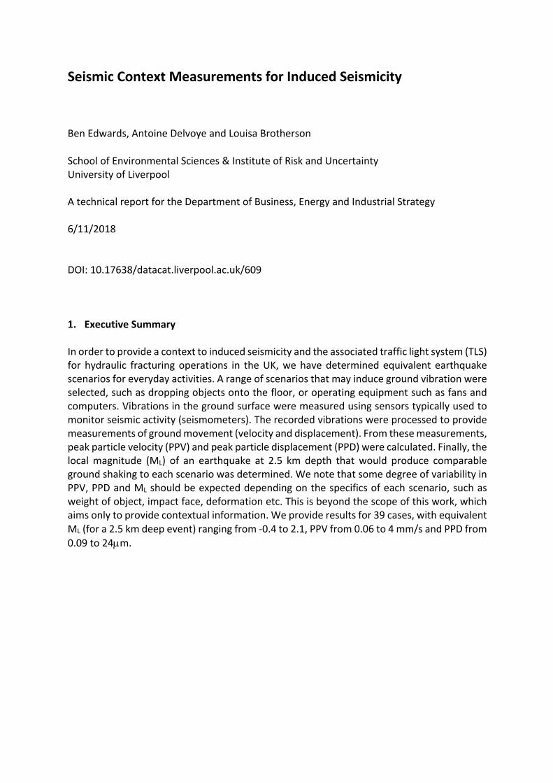
2. Data Acquisition and Processing Figure 1 shows some of the items used in this investigation. Where objects were dropped, they were allowed to fall under gravity from a height equivalent to a kitchen counter – about 0.9 – 1.0 m. Where items were bounced, the result is somewhat subjective as the force was not measured. In general, the seismometer was placed as close as possible (typically around 0.5 m) to the object (or the impact point). For traffic measurements, the seismometer was placed at the side of the road. Traffic measurements will vary significantly depending on the interaction of the traffic with the road surface (e.g. potholes, speedbumps). The road was judged to be smooth in this case so vibrations can be considered to be relatively low.

Figure 1: Items used for some of the scenarios.

Ground vibrations were recorded using a 3-component 4.5 Hz geophone (HL-6B) and DiGOS DATA-CUBE³ recording at 200 samples per second. All records were made on the vertical component consistent with the scenarios used to generate the waves (i.e. predominantly downward forces). Due to the nature of the experiment and the purpose—which is to provide a context to induced seismicity—the scenarios are somewhat subjective and should be interpreted within these constraints. For instance, dropped objects were always dropped from a height of ~1 m, but the orientation of the object, and its impact face was not controlled. Due to time constraints each scenario was performed once and therefore no scenario variability is determined. Linear detrending of the recorded data is performed, followed by the application of a 5% time-domain taper of the end samples. A cosine filter with bandpass 2 to 80 Hz is then applied prior to the removal of the instrument response function. Manufacturer information was used for instrument response restitution, providing direct measurements of ground vibration in (i) velocity and (ii) displacement in the range 2 to 80 Hz.


3

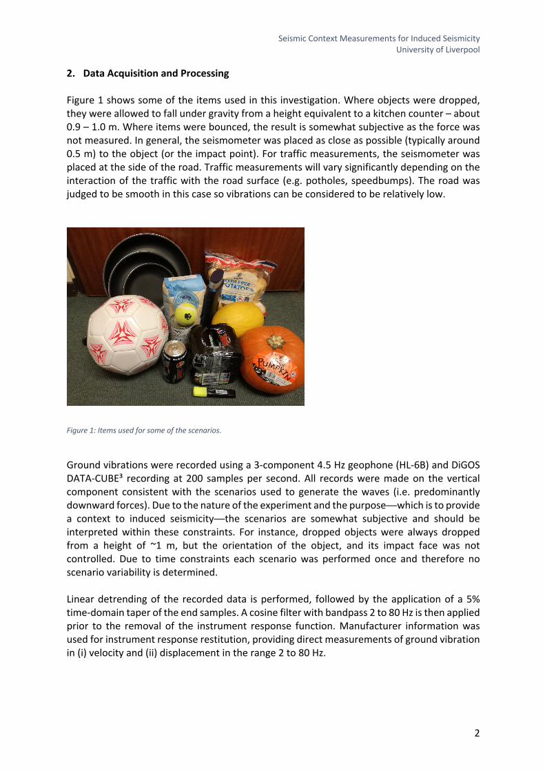
3. Calculation of PPV, PPD, ML Using the vibration time series, the (vertical) peak particle velocity and displacement are determined by searching for the largest absolute deviation from zero on the velocity and displacement time series, respectively. ML is calculated using the standard approach of the British Geological Survey (BGS). First the displacement time-history is convolved with the normalized response (i.e. without the x2080 gain) of a Wood-Anderson Seismometer (defined by its poles and zeros: [-5.49779+5.60886j], [-5.49779-5.60886j] and [0+0j], [0+0j] respectively) then the peak value,𝐴, is obtained in nm. Again, we work only with the vertical component of vibration since this is the strongest signal and more likely to be ‘felt’. This differs from the determination of ML for earthquakes, where the horizontal components of recording are used (earthquakes tend to generate the strongest shaking in the horizontal orientation). ML is defined by BGS (pers. comm. BGS) as: 𝑀𝐿 = log(𝐴) + 1.11 log(𝑟) + 0.00189𝑟 − 1.16𝑒56.78 − 2.09 (1) with 𝑟 in km. Using the measured peak amplitude, 𝐴, and defining ‘characteristic’ distance we can then determine an equivalent ML for our scenarios. For the distance we use 2.5 km, corresponding to being directly above a typical hydraulic fracturing well. For increasing distance the equivalent magnitude would increase – since the earthquake has to be larger in order to achieve the same level of vibrations further away. However, since the ground motions from induced seismicity are, in general, only felt in the epicentral region, we believe our measurements should be put into the context of being at the epicentre. 4. Scenario Results A summary of the results from all 39 scenarios is provided in Table 1. In the appendix, the waveforms for each scenario are shown. Note that higher ML does not necessarily imply higher peak velocity – since ML is a displacement-based measure. Table 1: Summary of PPV, PPD and ML for all scenarios, ordered by increasing ML

Description PPV

(mm/s) PPD (mm) A(nm) [email protected] Bus passing on opposite side of the road 0.014 0.000094 90.6 -0.4 Washing machine on wash cycle 0.006 0.000094 99.22 -0.4 Phone vibrating 0.009 0.000154 126.98 -0.2 Small car passing (nearside) 0.039 0.000156 161.08 -0.1 Washing machine on spin cycle 0.011 0.000207 179.42 -0.1 Train passing below (tunnel) 0.026 0.000191 192.37 -0.1 Closing a window 0.037 0.000211 206.91 0.0 Delivery van arriving 0.032 0.000206 238.75 0.0 Dropping a small frying pan 0.015 0.000285 396.94 0.3 A coach passing (nearside) 0.176 0.000564 583.42 0.4 Mixed traffic (busy road) 0.184 0.000612 622.59 0.5 A door slamming 0.281 0.000871 859.53 0.6 Sitting down on an office chair 0.039 0.001116 885.95 0.6 Building site (piledriver 15 m away) 0.235 0.000977 1126.22 0.7


4

Description PPV

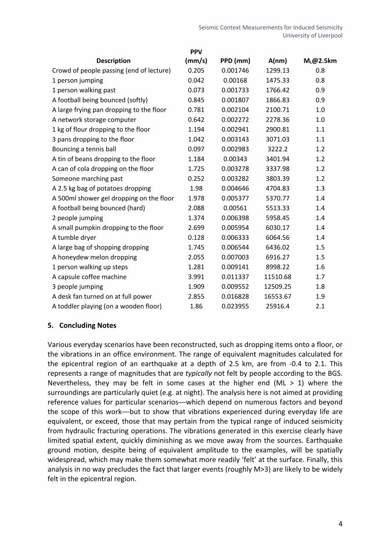
(mm/s) PPD (mm) A(nm) [email protected] Crowd of people passing (end of lecture) 0.205 0.001746 1299.13 0.8 1 person jumping 0.042 0.00168 1475.33 0.8 1 person walking past 0.073 0.001733 1766.42 0.9 A football being bounced (softly) 0.845 0.001807 1866.83 0.9 A large frying pan dropping to the floor 0.781 0.002104 2100.71 1.0 A network storage computer 0.642 0.002272 2278.36 1.0 1 kg of flour dropping to the floor 1.194 0.002941 2900.81 1.1 3 pans dropping to the floor 1.042 0.003143 3071.03 1.1 Bouncing a tennis ball 0.097 0.002983 3222.2 1.2 A tin of beans dropping to the floor 1.184 0.00343 3401.94 1.2 A can of cola dropping on the floor 1.725 0.003278 3337.98 1.2 Someone marching past 0.252 0.003282 3803.39 1.2 A 2.5 kg bag of potatoes dropping 1.98 0.004646 4704.83 1.3 A 500ml shower gel dropping on the floor 1.978 0.005377 5370.77 1.4 A football being bounced (hard) 2.088 0.00561 5513.33 1.4 2 people jumping 1.374 0.006398 5958.45 1.4 A small pumpkin dropping to the floor 2.699 0.005954 6030.17 1.4 A tumble dryer 0.128 0.006333 6064.56 1.4 A large bag of shopping dropping 1.745 0.006544 6436.02 1.5 A honeydew melon dropping 2.055 0.007003 6916.27 1.5 1 person walking up steps 1.281 0.009141 8998.22 1.6 A capsule coffee machine 3.991 0.011337 11510.68 1.7 3 people jumping 1.909 0.009552 12509.25 1.8 A desk fan turned on at full power 2.855 0.016828 16553.67 1.9 A toddler playing (on a wooden floor) 1.86 0.023955 25916.4 2.1

5. Concluding Notes Various everyday scenarios have been reconstructed, such as dropping items onto a floor, or the vibrations in an office environment. The range of equivalent magnitudes calculated for the epicentral region of an earthquake at a depth of 2.5 km, are from -0.4 to 2.1. This represents a range of magnitudes that are typically not felt by people according to the BGS. Nevertheless, they may be felt in some cases at the higher end (ML > 1) where the surroundings are particularly quiet (e.g. at night). The analysis here is not aimed at providing reference values for particular scenarios—which depend on numerous factors and beyond the scope of this work—but to show that vibrations experienced during everyday life are equivalent, or exceed, those that may pertain from the typical range of induced seismicity from hydraulic fracturing operations. The vibrations generated in this exercise clearly have limited spatial extent, quickly diminishing as we move away from the sources. Earthquake ground motion, despite being of equivalent amplitude to the examples, will be spatially widespread, which may make them somewhat more readily ‘felt’ at the surface. Finally, this analysis in no way precludes the fact that larger events (roughly M>3) are likely to be widely felt in the epicentral region.


5

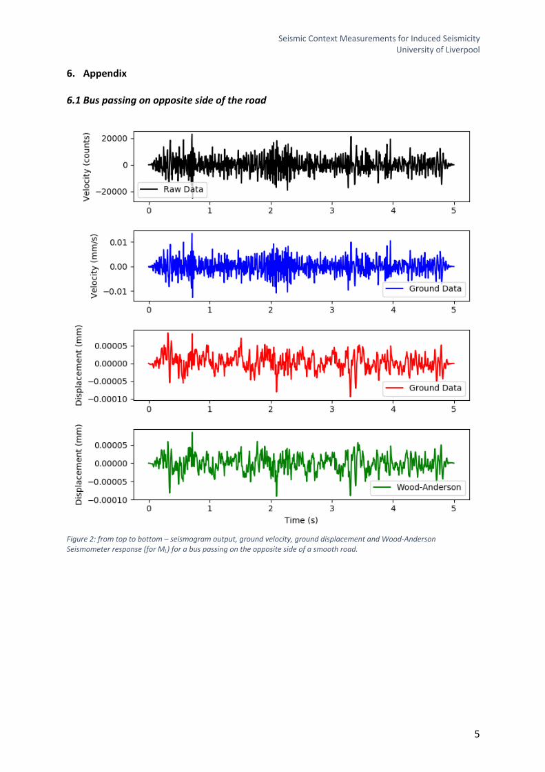
6. Appendix 6.1 Bus passing on opposite side of the road

Figure 2: from top to bottom – seismogram output, ground velocity, ground displacement and Wood-Anderson Seismometer response (for ML) for a bus passing on the opposite side of a smooth road.


6

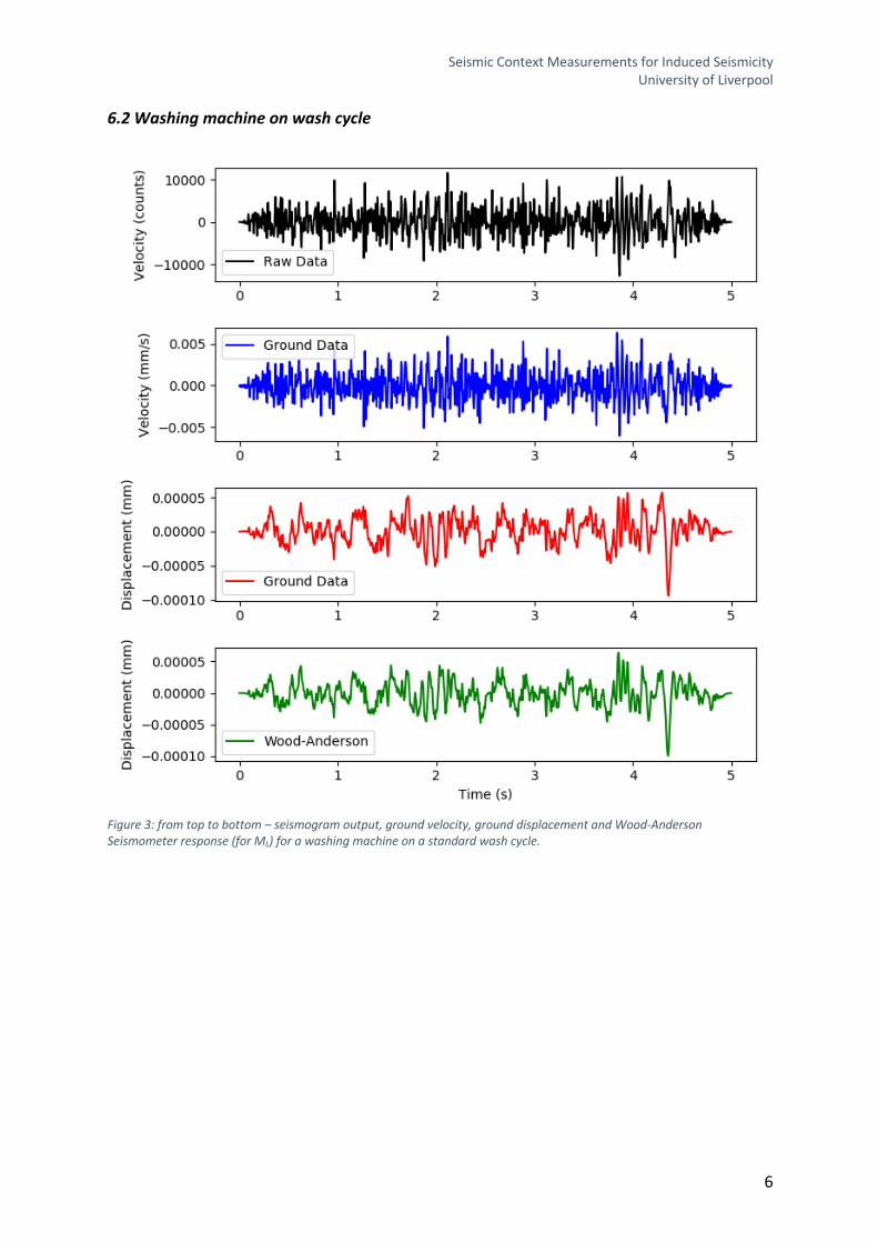
6.2 Washing machine on wash cycle

Figure 3: from top to bottom – seismogram output, ground velocity, ground displacement and Wood-Anderson Seismometer response (for ML) for a washing machine on a standard wash cycle.


7

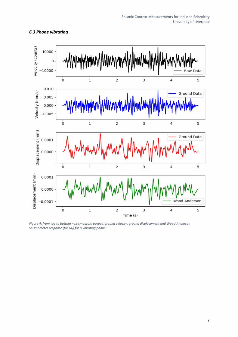
6.3 Phone vibrating

Figure 4: from top to bottom – seismogram output, ground velocity, ground displacement and Wood-Anderson Seismometer response (for ML) for a vibrating phone.


8

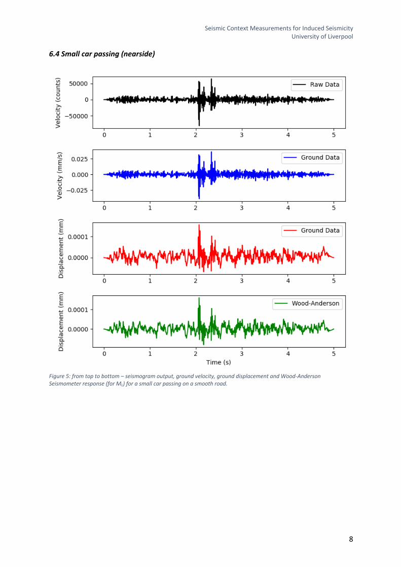
6.4 Small car passing (nearside)

Figure 5: from top to bottom – seismogram output, ground velocity, ground displacement and Wood-Anderson Seismometer response (for ML) for a small car passing on a smooth road.


9

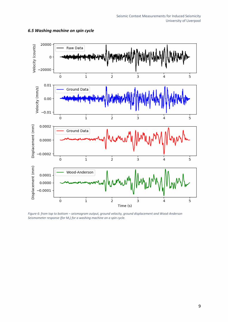
6.5 Washing machine on spin cycle

Figure 6: from top to bottom – seismogram output, ground velocity, ground displacement and Wood-Anderson Seismometer response (for ML) for a washing machine on a spin cycle.


10

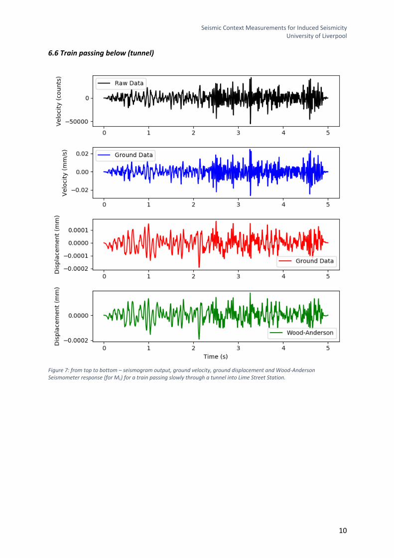
6.6 Train passing below (tunnel)

Figure 7: from top to bottom – seismogram output, ground velocity, ground displacement and Wood-Anderson Seismometer response (for ML) for a train passing slowly through a tunnel into Lime Street Station.


11

6.7 Closing a window

Figure 8: from top to bottom – seismogram output, ground velocity, ground displacement and Wood-Anderson Seismometer response (for ML) for a window being closed.


12

6.8 Delivery van arriving

Figure 9: from top to bottom – seismogram output, ground velocity, ground displacement and Wood-Anderson Seismometer response (for ML) for the arrival of a delivery van.


13

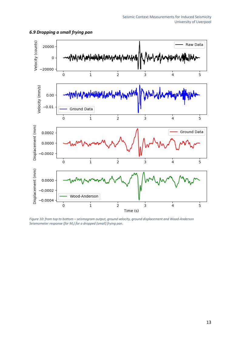
6.9 Dropping a small frying pan

Figure 10: from top to bottom – seismogram output, ground velocity, ground displacement and Wood-Anderson Seismometer response (for ML) for a dropped (small) frying pan.


14

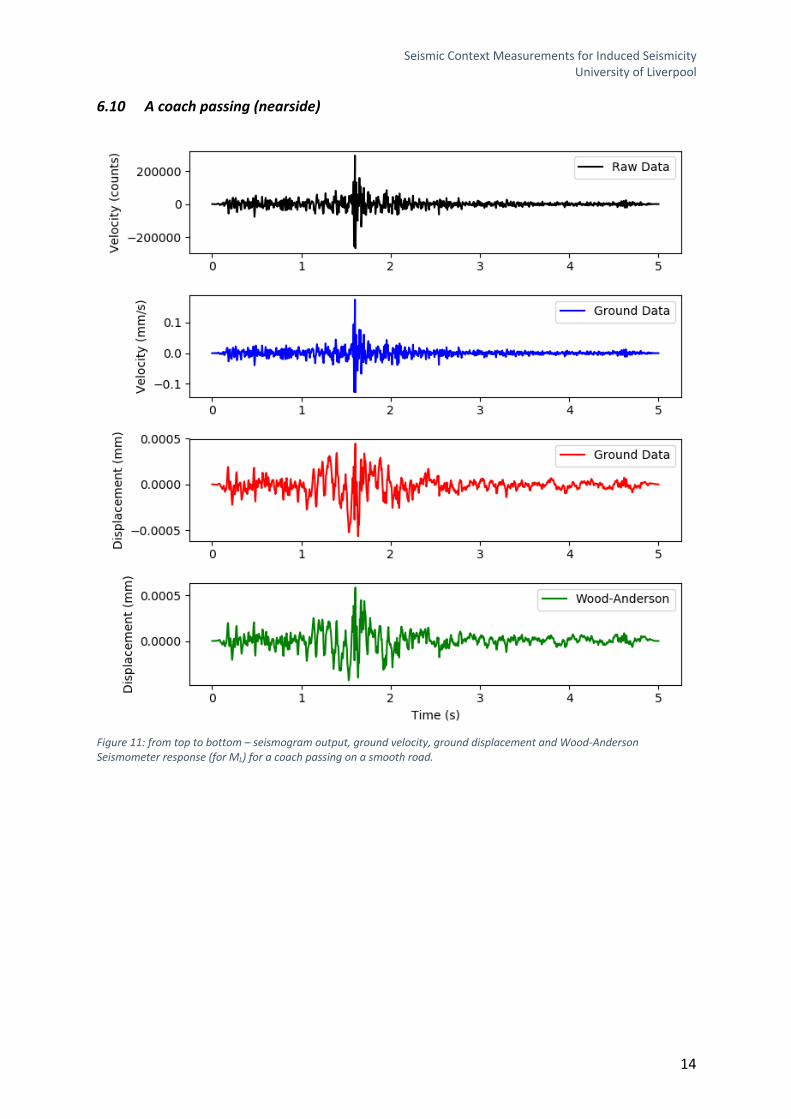
6.10 A coach passing (nearside)

Figure 11: from top to bottom – seismogram output, ground velocity, ground displacement and Wood-Anderson Seismometer response (for ML) for a coach passing on a smooth road.


15

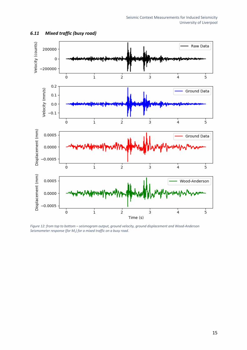
6.11 Mixed traffic (busy road)

Figure 12: from top to bottom – seismogram output, ground velocity, ground displacement and Wood-Anderson Seismometer response (for ML) for a mixed traffic on a busy road.


16

6.12 A door slamming

Figure 13: from top to bottom – seismogram output, ground velocity, ground displacement and Wood-Anderson Seismometer response (for ML) for a door being slammed.


17

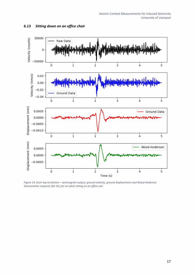
6.13 Sitting down on an office chair

Figure 14: from top to bottom – seismogram output, ground velocity, ground displacement and Wood-Anderson Seismometer response (for ML) for an adult sitting on an office cair.


18

6.14 Building site (piledriver 15 m away)

Figure 15: from top to bottom – seismogram output, ground velocity, ground displacement and Wood-Anderson Seismometer response (for ML) for a building site with piledriver approx. 15 m away.


19

6.15 Crowd of people passing (end of lecture)

Figure 16: from top to bottom – seismogram output, ground velocity, ground displacement and Wood-Anderson Seismometer response (for ML) for a crowd of adults passing.


20

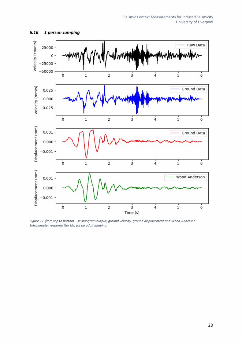
6.16 1 person Jumping

Figure 17: from top to bottom – seismogram output, ground velocity, ground displacement and Wood-Anderson Seismometer response (for ML) for an adult jumping.


21

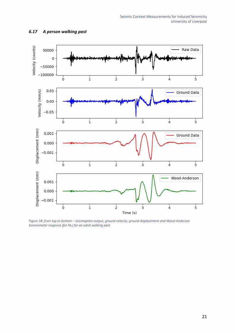
6.17 A person walking past

Figure 18: from top to bottom – seismogram output, ground velocity, ground displacement and Wood-Anderson Seismometer response (for ML) for an adult walking past.


22

6.18 A football being bounced (softly)

Figure 19: from top to bottom – seismogram output, ground velocity, ground displacement and Wood-Anderson Seismometer response (for ML) for a football being bounced.


23

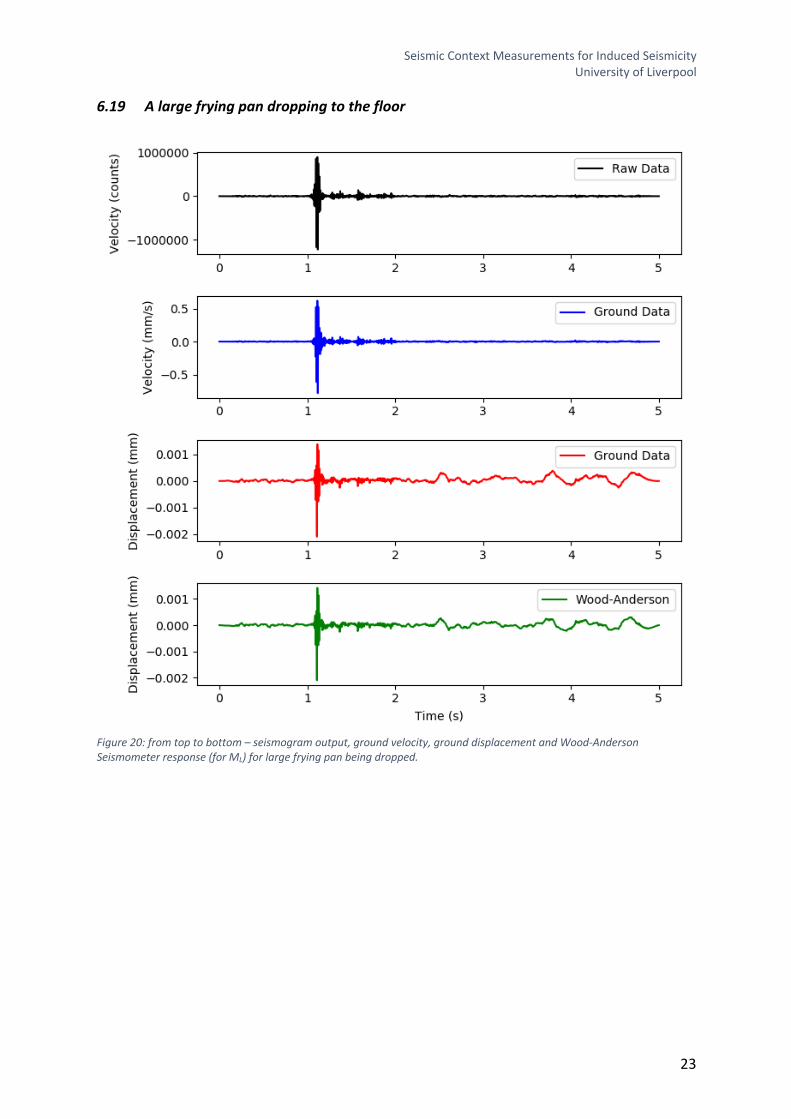
6.19 A large frying pan dropping to the floor

Figure 20: from top to bottom – seismogram output, ground velocity, ground displacement and Wood-Anderson Seismometer response (for ML) for large frying pan being dropped.


24

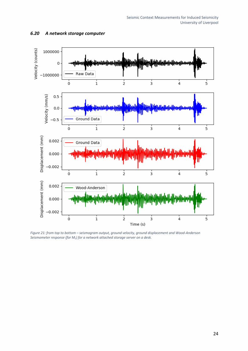
6.20 A network storage computer

Figure 21: from top to bottom – seismogram output, ground velocity, ground displacement and Wood-Anderson Seismometer response (for ML) for a network attached storage server on a desk.


25

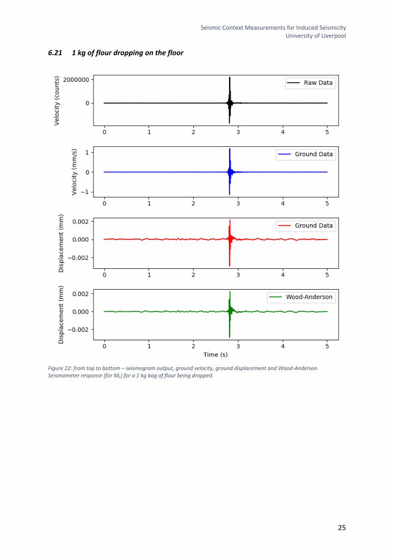
6.21 1 kg of flour dropping on the floor

Figure 22: from top to bottom – seismogram output, ground velocity, ground displacement and Wood-Anderson Seismometer response (for ML) for a 1 kg bag of flour being dropped.


26

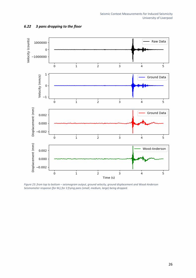
6.22 3 pans dropping to the floor

Figure 23: from top to bottom – seismogram output, ground velocity, ground displacement and Wood-Anderson Seismometer response (for ML) for 3 frying pans (small, medium, large) being dropped.


27

6.23 Bouncing a tennis ball

Figure 24: from top to bottom – seismogram output, ground velocity, ground displacement and Wood-Anderson Seismometer response (for ML) for tennis ball being bounced.


28

6.24 A tin of beans dropping to the floor

Figure 25: from top to bottom – seismogram output, ground velocity, ground displacement and Wood-Anderson Seismometer response (for ML) for a tin of beans being dropped.


29

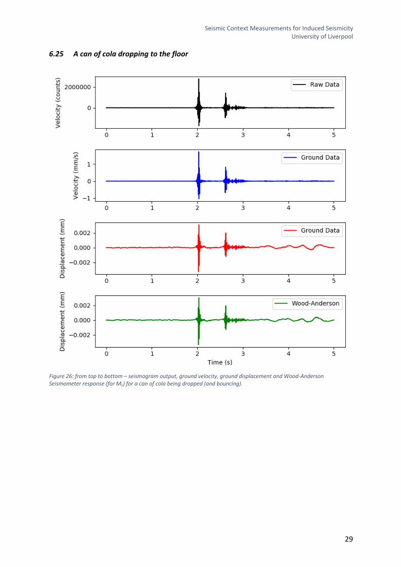
6.25 A can of cola dropping to the floor

Figure 26: from top to bottom – seismogram output, ground velocity, ground displacement and Wood-Anderson Seismometer response (for ML) for a can of cola being dropped (and bouncing).


30

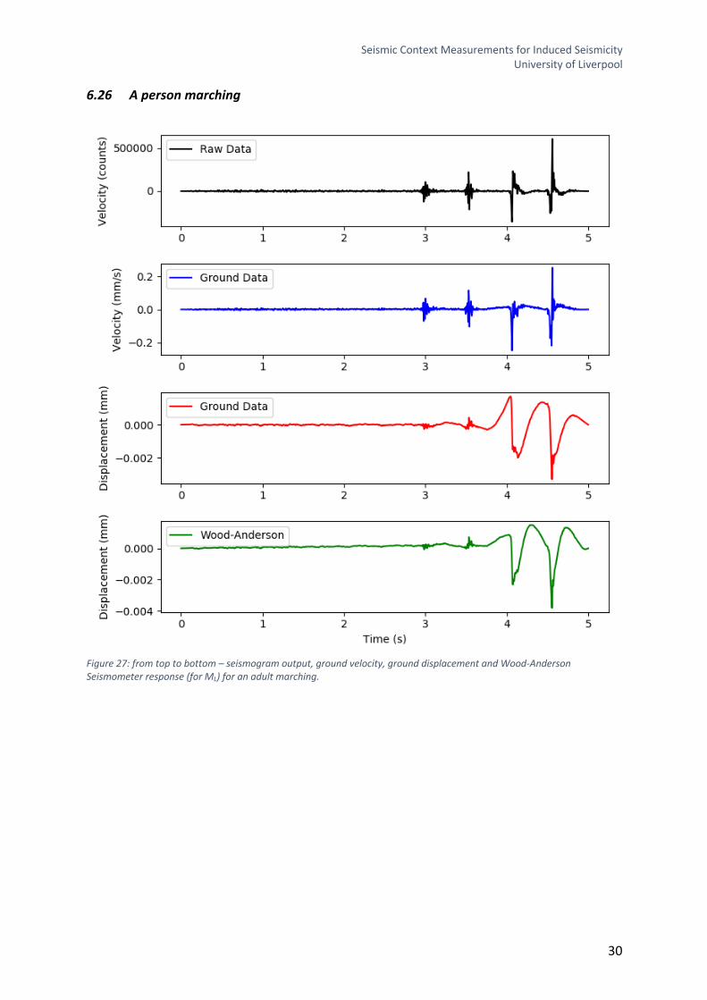
6.26 A person marching

Figure 27: from top to bottom – seismogram output, ground velocity, ground displacement and Wood-Anderson Seismometer response (for ML) for an adult marching.


31

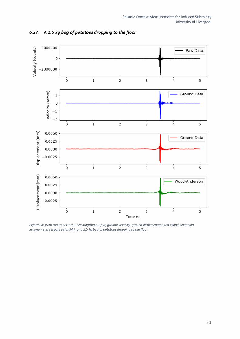
6.27 A 2.5 kg bag of potatoes dropping to the floor

Figure 28: from top to bottom – seismogram output, ground velocity, ground displacement and Wood-Anderson Seismometer response (for ML) for a 2.5 kg bag of potatoes dropping to the floor.


32

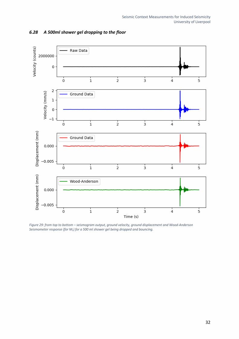
6.28 A 500ml shower gel dropping to the floor

Figure 29: from top to bottom – seismogram output, ground velocity, ground displacement and Wood-Anderson Seismometer response (for ML) for a 500 ml shower gel being dropped and bouncing.


33

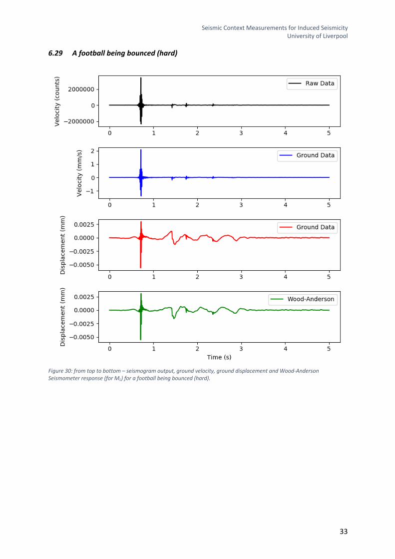
6.29 A football being bounced (hard)

Figure 30: from top to bottom – seismogram output, ground velocity, ground displacement and Wood-Anderson Seismometer response (for ML) for a football being bounced (hard).


34

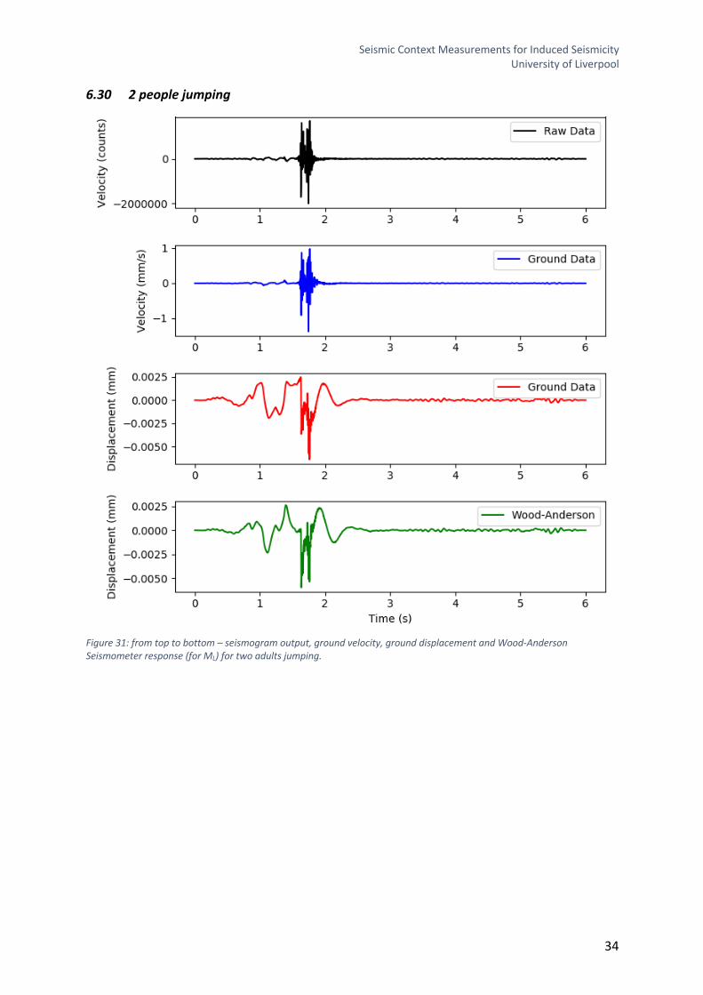
6.30 2 people jumping

Figure 31: from top to bottom – seismogram output, ground velocity, ground displacement and Wood-Anderson Seismometer response (for ML) for two adults jumping.


35

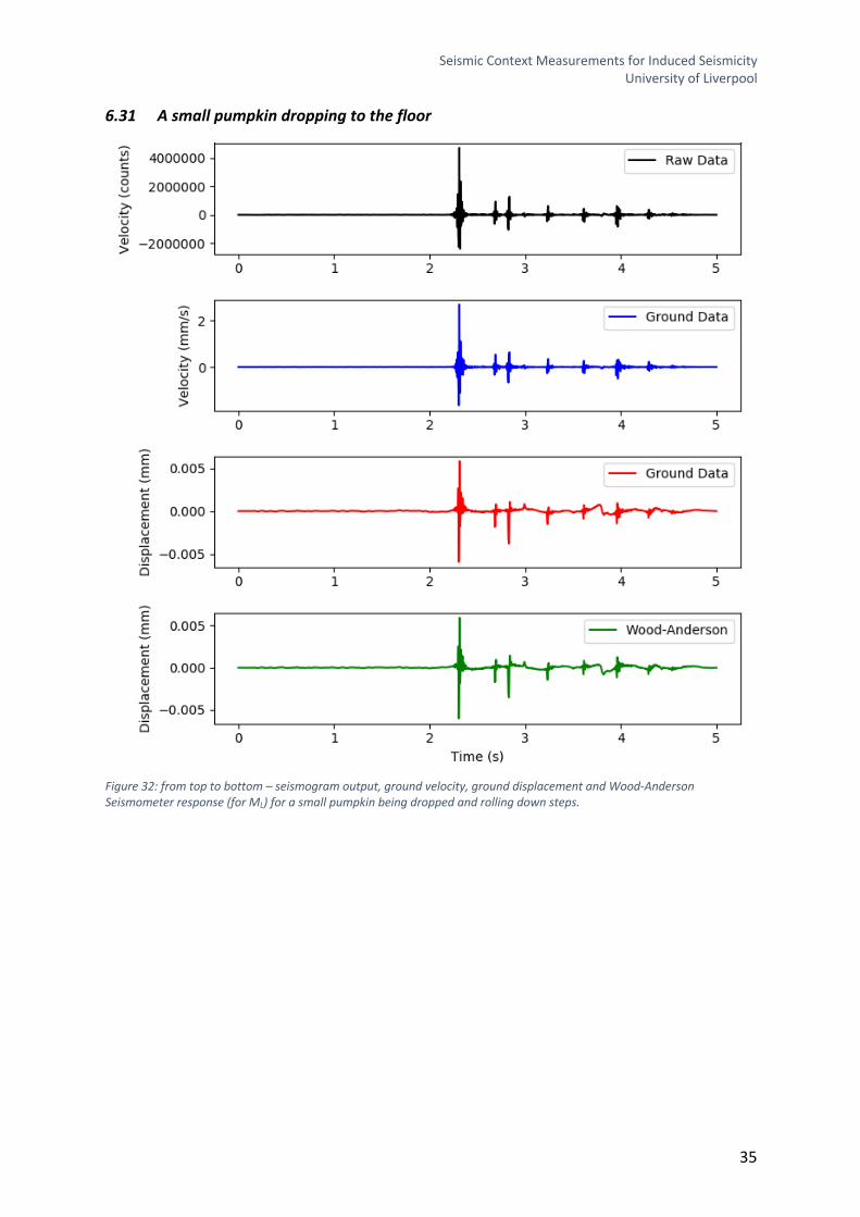
6.31 A small pumpkin dropping to the floor

Figure 32: from top to bottom – seismogram output, ground velocity, ground displacement and Wood-Anderson Seismometer response (for ML) for a small pumpkin being dropped and rolling down steps.


36

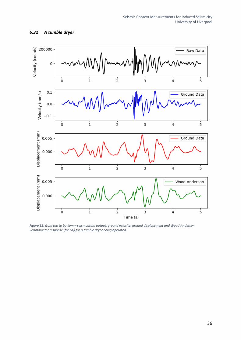
6.32 A tumble dryer

Figure 33: from top to bottom – seismogram output, ground velocity, ground displacement and Wood-Anderson Seismometer response (for ML) for a tumble dryer being operated.


37

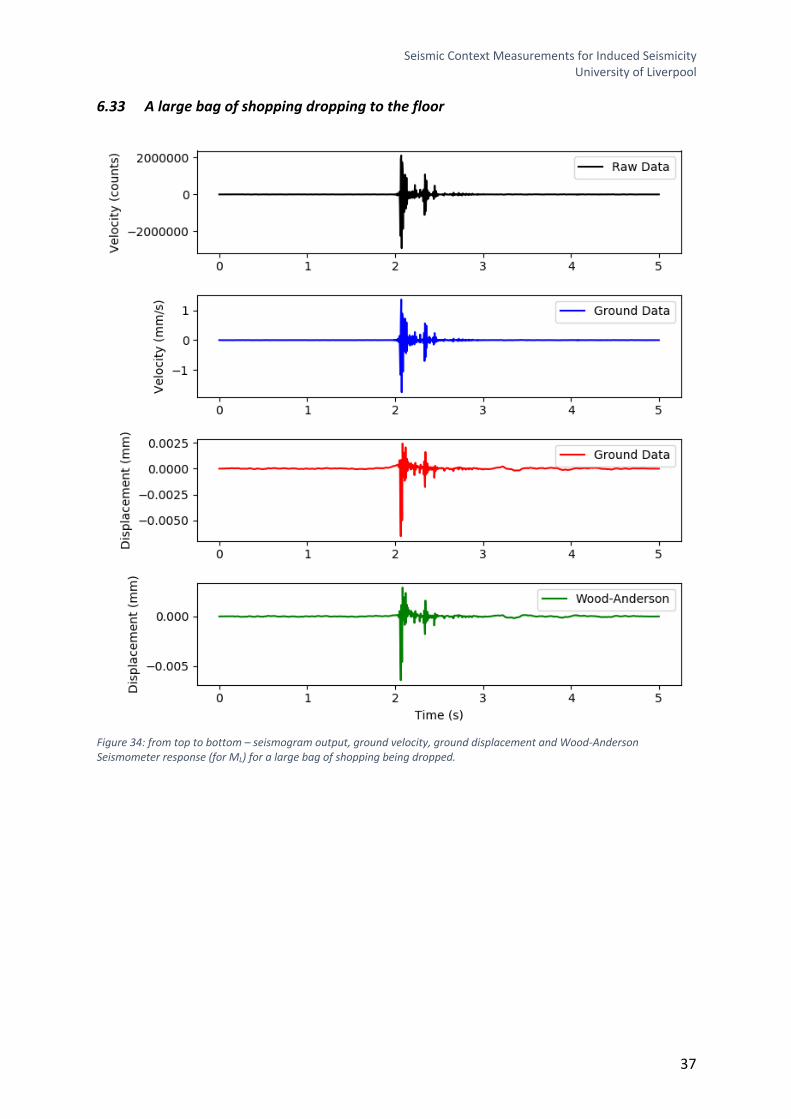
6.33 A large bag of shopping dropping to the floor

Figure 34: from top to bottom – seismogram output, ground velocity, ground displacement and Wood-Anderson Seismometer response (for ML) for a large bag of shopping being dropped.


38

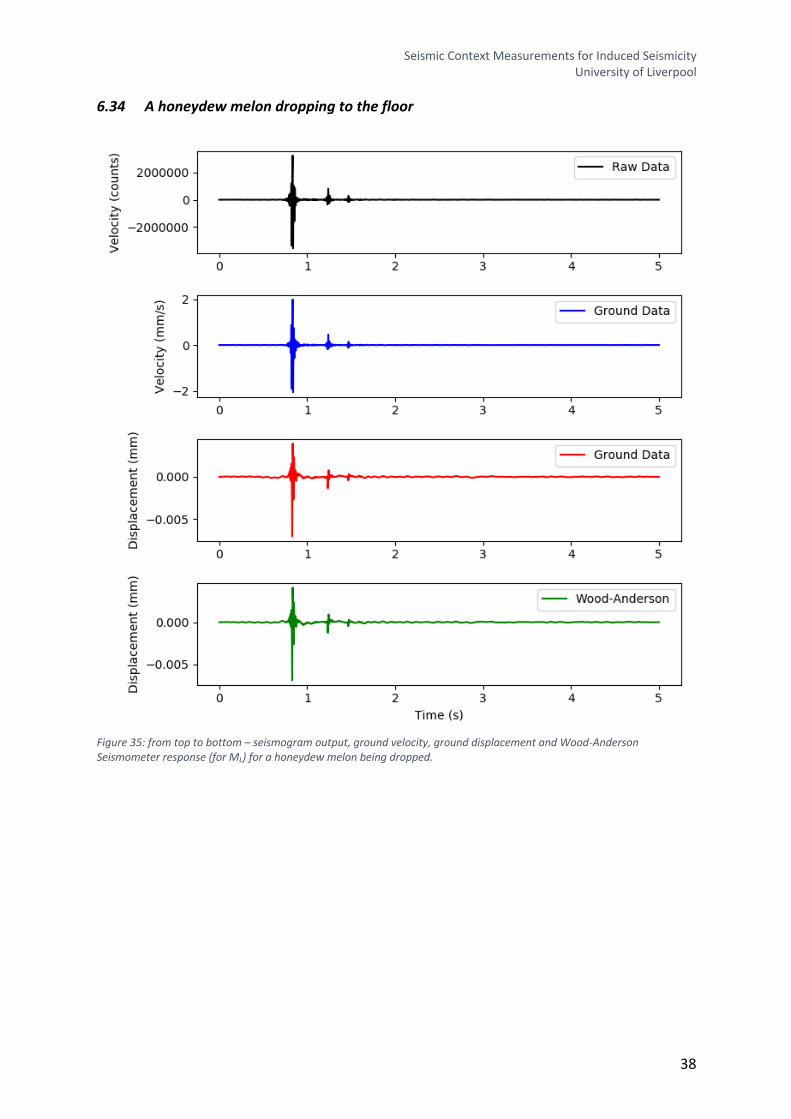
6.34 A honeydew melon dropping to the floor

Figure 35: from top to bottom – seismogram output, ground velocity, ground displacement and Wood-Anderson Seismometer response (for ML) for a honeydew melon being dropped.


39

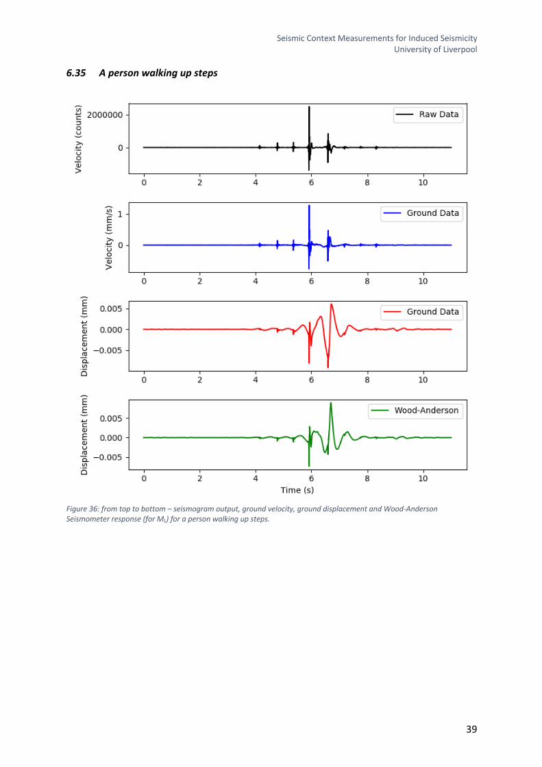
6.35 A person walking up steps

Figure 36: from top to bottom – seismogram output, ground velocity, ground displacement and Wood-Anderson Seismometer response (for ML) for a person walking up steps.


40

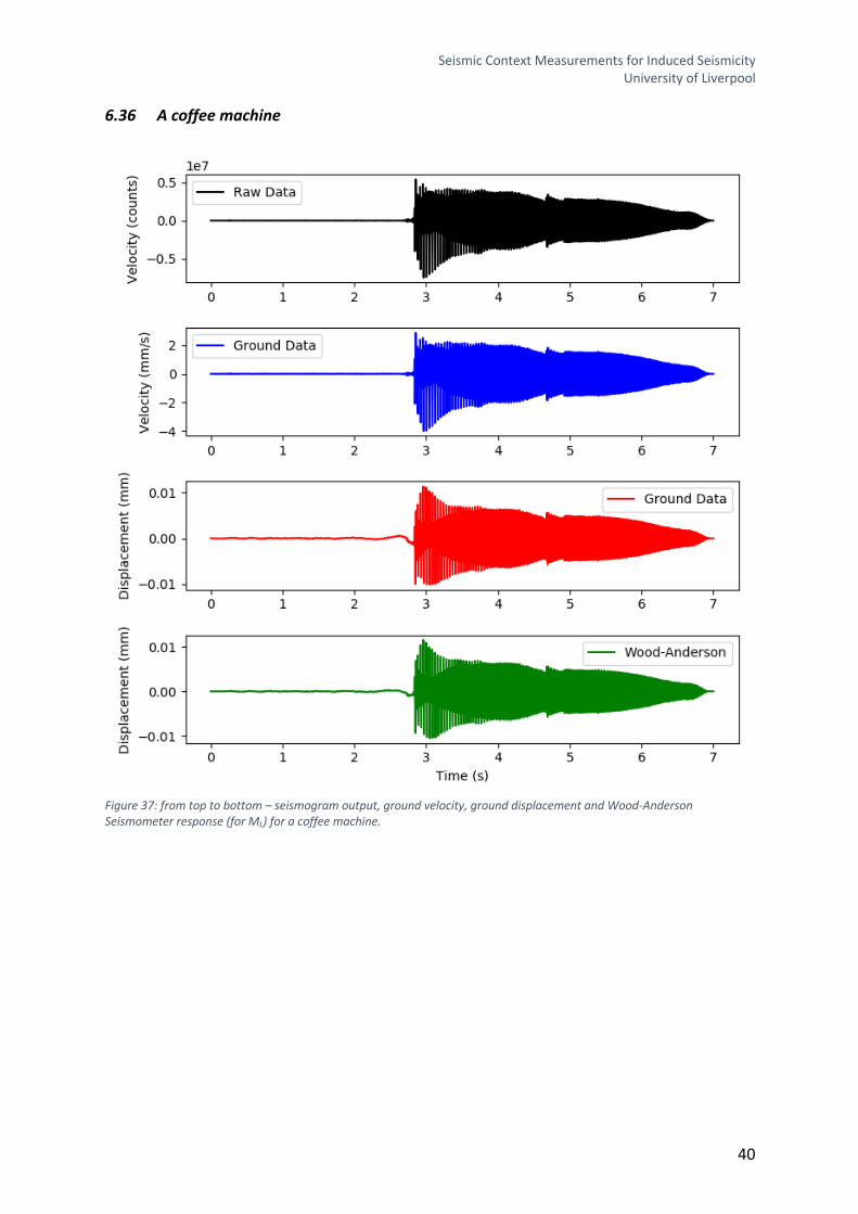
6.36 A coffee machine

Figure 37: from top to bottom – seismogram output, ground velocity, ground displacement and Wood-Anderson Seismometer response (for ML) for a coffee machine.


41

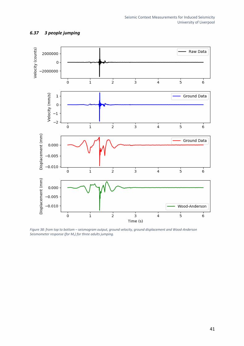
6.37 3 people jumping

Figure 38: from top to bottom – seismogram output, ground velocity, ground displacement and Wood-Anderson Seismometer response (for ML) for three adults jumping.


42

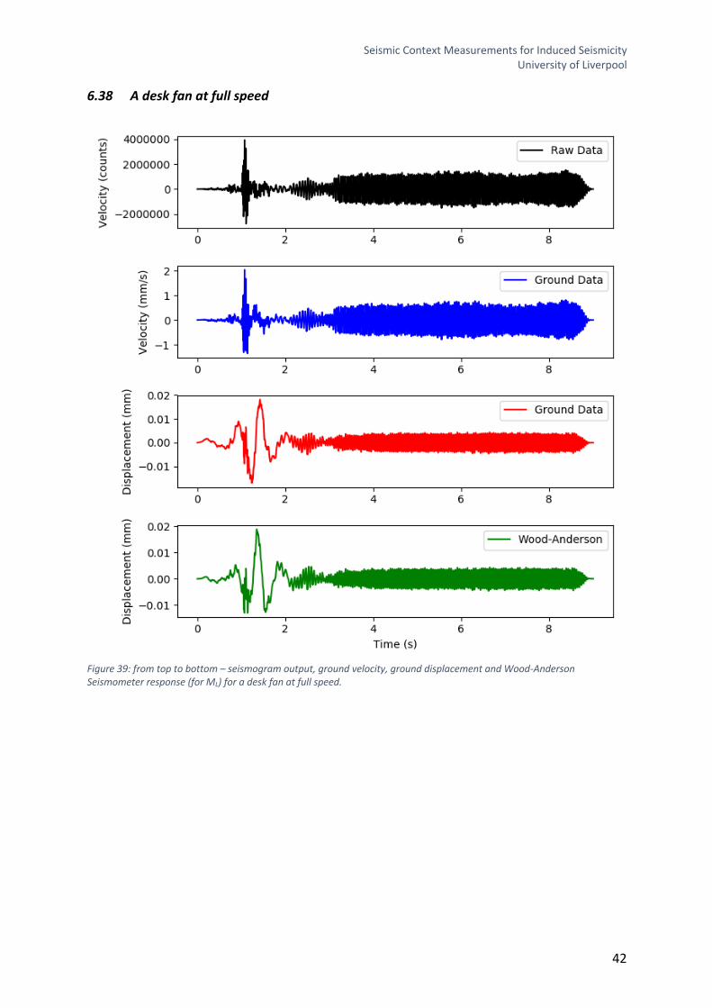
6.38 A desk fan at full speed

Figure 39: from top to bottom – seismogram output, ground velocity, ground displacement and Wood-Anderson Seismometer response (for ML) for a desk fan at full speed.


43

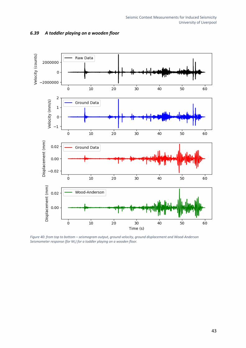
6.39 A toddler playing on a wooden floor

Figure 40: from top to bottom – seismogram output, ground velocity, ground displacement and Wood-Anderson Seismometer response (for ML) for a toddler playing on a wooden floor.

Documents

Seismic Context Measurements - University of Liverpool