Segment Profitability and the Proprietary Costs of Disclosure

Philip G. Berger Graduate School of Business, University of Chicago, 1101 E. 58th St., Chicago, IL 60637

and

Rebecca N. Hann*

Leventhal School of Accounting, University of Southern California, Los Angeles, CA 90089

April, 2005

*Corresponding Author. Leventhal School of Accounting University of Southern California Los Angeles, CA 90089-1421 Phone: (213) 740-6939 Fax: (213) 747-2815 email: rebecca.hann@marshall.usc.edu

We have benefited from the comments of Ray Ball, Anne Beatty, Bill Beaver, Bob Bowen, John Dickhaut, Ted Goodman, Il-Horn Hann, Leslie Hodder, Ole-Kristian Hope, Jack Hughes, Bjorn Jorgensen, S.P. Kothari, Christian Leuz, Maureen McNichols, Greg Miller, Joe Piotroski, Gord Richardson, Tjomme Rusticus, Shiva Rajgopal, Terry Shevlin, Abbie Smith, Suraj Srinivasan, Andy Van Buskirk, Ram Venkataraman, Ro Verrecchia, Joe Weber, and workshop participants at the following universities: Chicago, Minnesota, Toronto, Washington and Stanford Accounting Summer Camp. We also thank James Chan, Steffi Chan, Jae Kim, and Pierre Sato for their research assistance. Berger gratefully acknowledges financial support from the Neubauer Family Faculty Fellows program at the University of Chicago Graduate School of Business.

Segment Profitability and the Proprietary Costs of Disclosure

Abstract: We exploit the new U.S. segment reporting standard, SFAS 131, to identify a sample of firms

that increased segment disaggregation solely due to a mandated reporting change. We then test the joint

hypothesis that: (1) the increase in segment reporting under the new rule indicates discretionary

aggregation of segments under the old standard (SFAS 14) and (2) concerns about revealing profitability

information motivated managers to aggregate segment data under the old reporting regime.

We find firms increased their segment disclosure on adoption of the new rule when they had a higher

level of abnormal profitability, a slower rate of deterioration in abnormal profitability, and operations

with more divergent profit performance. These findings are consistent with firms being less likely to

voluntarily disaggregate segment information when the proprietary costs of additional disaggregation are

higher. We do not find, however, a significant decline in abnormal profits for the firms that increased

segment disaggregation after adoption of the new rule. One possible explanation is that the proprietary

costs of the mandated increase in segment disaggregation are offset by the proprietary information

benefits of concurrent reporting increases by competitors. A second possibility, for which we find some

preliminary support, is that agency costs as well as proprietary costs motivated the aggregation of

segment information under the old rule.

Keywords: segment reporting; discretionary disclosure; proprietary costs; agency costs

Data Availability: All data are available from public sources, except for the restated SFAS 131 segment data, which are proprietary.

1

1. Introduction

This paper exploits the recent change in U.S. segment reporting rules to examine whether the desire to

conceal profitability data reduces voluntary disclosure and, relatedly, whether a mandated increase in

disclosure erodes profitability. Information about profitability is potentially valuable to both capital

market participants and the firm’s competitors. Indeed, mandated changes aimed at increasing

disclosures about profitability are often supported by capital market participants while being opposed by

managers. Our goal in this paper is to study whether the proprietary cost argument for opposing a

mandated increase in disclosure finds empirical support.

A mandated reporting change offers several advantages for studying whether the desire to withhold

profitability data reduces disclosure. If the mandated change tends to increase disclosure it provides an

indication that there were important costs of voluntarily disclosing the information under the old reporting

rule. Moreover, a mandated change is much less likely than a voluntary one to be endogenously related

to profitability measures (or other variables of interest). This allows us to examine profitability as both an

explanatory variable for the voluntary disclosure decisions made prior to the rule change and as a

dependent variable potentially affected by the mandated disclosure change.

The mandated change we examine is the new segment reporting required by SFAS 131, which

supercedes SFAS 14.1 The adoption of the new standard was largely motivated by the belief that

disaggregation of segment data has large capital market benefits. Consistent with this view, most sell-

side analysts consider segment disclosures (followed by the three financial statements) as the most useful

data for their investment recommendations (Epstein and Palepu 1999). Despite the importance of

segment information to capital market participants, segment disaggregation was often criticized for being

limited under SFAS 14’s industry approach. A major concern was that discretion in the definition of

“industry” allowed many enterprises to report much less segment information to external users than what

was reported internally (Ernst & Young 1998). Hence, the main objective of Statement 131 was to

1 SFAS 131 is FASB Statement No. 131, Disclosures about Segments of an Enterprise and Related Information (FASB 1997). SFAS 14 is FASB Statement No. 14, Financial Reporting for Segments of a Business Enterprise (FASB 1976).

2

increase segment disaggregation. Recent studies (Street et al. 2000; Herrmann and Thomas 2000; Berger

and Hann 2003) provide evidence that the new rule induced firms to provide more disaggregated segment

information. The increase in disaggregation was primarily attributable to Statement 131 defining

segments based on the firm’s internal decision-making structure rather than on the basis of industry.

We acknowledge that the greater aggregation of segments under SFAS 14 could merely indicate that

firms use internal decision-making structures that partition the firm more finely than a neutral application

of the industry-based definition of segments. However, our maintained assumption is that many firms

opportunistically exploited the flexibility afforded by Statement 14 to broadly define their operating

segments. If the aggregation of segments was indeed due to management discretion, a natural question

that follows is: What motivated managers to withhold disaggregated segment information under the old

reporting regime? We therefore explore the joint hypothesis that aggregation of segments under SFAS 14

reflects “hiding” of segment information (rather than a “neutral” grouping of operations into industries)

and that the motivation was to withhold information about profitability.

Managers have often expressed concerns that more segment disclosure would force them to provide

valuable proprietary information to competitors. Ettredge, Kwon, and Smith (2002) report that 86% of

the (self-selected) industrial firms that commented on the exposure draft for SFAS 131 were opposed to

the new standard on the grounds that “it would put them at competitive disadvantage.” Of course, even if

the lobbying against the new rule were attributable more to managers’ self-interests than to shareholders’

interests, managers would be unlikely to say so in their lobbying letters. More direct evidence about the

proprietary cost motive is thus called for. We gather such evidence by using a hand-collected database

that contains the restated SFAS 131 segment data for the final SFAS 14 fiscal year. This database allows

us to compare the segment information generated under the two reporting regimes for the same firm at the

same time and thus to identify the firms that have increased segment disclosure solely because of the

mandated reporting change.

Further, the mandated segment reporting change allows us to identify a sample of firms where the

proprietary costs of disclosure likely outweigh the capital market benefits. Under the new standard,

3

enterprises are required to present disaggregated information based on how management internally

evaluates the operating performance of its business units. Because the segment data required under the

new standard were presumably already available internally, managers could have voluntarily disclosed

more disaggregated information with little data collection cost under the old reporting regime.

Because our research design relies on comparing the number of segments reported under SFAS 14 to

that reported under SFAS 131, we take steps to ensure that this is an “apples-to-apples” comparison. We

seek to compare line-of-business reporting under the two regimes. Therefore, we aggregate Statement

131 geographic segments within the same line-of-business and ignore Statement 14 geographic segments.

Moreover, to ensure that our restated SFAS 131 segments do not reflect restatement for reasons other than

adoption of Statement 131, we eliminate observations with restated data that reflect real changes in the

adoption year (e.g., pooling acquisitions or discontinued operations).

After taking these steps to achieve an apples-to-apples comparison, we make three validity checks of

our approach. First, our comparison of line-of-business reporting under the two standards relies on

Compustat’s assignment of SIC codes, which may seem more questionable under SFAS 131 because the

new standard does not define segments based on industry. However, time-series correlations between the

sales (earnings) of a segment and the sales (earnings) of the segment’s corresponding industry show no

difference between the two segment reporting regimes in the applicability of using Compustat SIC codes

to classify segments. Second, we identify 37 firms for which reporting more segments under Statement

131 could be attributable to internal growth rather than adoption of the new standard. Inferences are

unchanged when these 37 firms are excluded from the tests. Finally, we examine the validity of our

assumption that SFAS 131 segment data constitute new public disclosures by checking whether some of

these data were disclosed in the last SFAS 14 10-K’s MD&A. Both abnormal return tests around the

filing of the last Statement 14 10-K for the full sample and detailed examinations of the MD&A for a

subsample of 100 firms show the last SFAS 14 year’s MD&A contained little of the Statement 131

segment earnings information.

4

Our empirical results indicate that managers were more likely to increase the disaggregation of

segment information under Statement 131 when their firms had a large variation in segment performance,

high levels of abnormal profit, and operations in industries with a slow rate of decrease in abnormal

profitability. These results are consistent with firms being less likely to voluntarily disaggregate segment

information under Statement 14 when increased disaggregated disclosure would have revealed more

detailed information about the firm’s profit opportunities.

Although our evidence is consistent with proprietary cost concerns affecting segment aggregation

under SFAS 14, we do not find the firms that revealed more disaggregated information under the new

standard experienced a significant decline in abnormal profits. Taken together, these results suggest the

new standard forced some companies to disclose proprietary data, but that the information revealed did

not result in competitive harm. A possible explanation for these results is that firms that would suffer

competitive harm from voluntarily increasing segment disaggregation did not suffer harm when they were

mandated to increase disaggregation at the same time as many of their competitors.

An alternative explanation for the preceding results is that the measures we use to capture proprietary

information costs also capture (at least to some extent) agency costs. If the aggregation of segments

under Statement 14 was partly attributable to agency issues, it becomes less likely that abnormal

profitability should decrease after SFAS 131 mandated more disaggregation. Disaggregated segment

disclosure can provide information about resource transfers across segments and the presence of poorly

performing segments, both of which can attract heightened external monitoring. Our results show that the

presence of a loss segment and, to a lesser extent, a positive measure of cross-segment resource transfers

are associated with an increased probability of aggregating segments under SFAS 14.

The results for the proprietary cost measures continue to hold, however, even after including the

separate measures of agency costs that also significantly affect the segment aggregation decision. Our

evidence thus indicates that both proprietary costs and agency costs reduce voluntary disaggregation of

segment information. We leave to future research a more detailed exploration of the role played by

agency costs in the discretionary disclosure of segment data.

5

The rest of the paper is organized as follows. Section 2 provides a brief discussion of SFAS131 and

reviews the related literature. Section 3 presents the research hypotheses and section 4 details our sample

selection. Section 5 describes the research methods and presents our empirical results, with our

conclusions offered in section 6.

2. Background

2.1 SFAS 131

SFAS 131 was issued by the FASB in June 1997 and is effective for fiscal years commencing after

December 15, 1997. The main difference between SFAS 131 and SFAS 14 is in how a segment is

defined. Under SFAS 14, business segments were defined by industry groupings of products and services

sold to external customers. In contrast, SFAS 131 defines segments based on how management organizes

divisions within the enterprise for making decisions and assessing performance. The management

approach along with the other provisions of SFAS 131 offers several trade-offs relative to SFAS 14's

industry approach. Most fundamentally, the new standard provides greater, but more individualized,

insight into the management strategy of each firm, thus reflecting a trade-off between more relevance and

less comparability. The FASB favored the new approach over the old primarily because of its belief that

the new standard provides more relevant and disaggregated information to users.

The most frequent criticism of SFAS 14 was its loose definition of “industry,” which allowed

managers of some diversified firms to report all operations “as being in a single, very broadly defined

industry segment” (FAS 131, ¶ 58). The FASB believed that the management approach would offer less

discretion about segment definition and that, as a result, the information provided under SFAS 131 would

be less subjective than what was provided under the industry approach.2 Therefore, the FASB expected

the new standard to induce more segmentation.

2 Critics argued, however, that the new standard's aggregation criteria still allow for some discretion by managers in deciding how many segments to report. Under the new standard, multiple operating segments can be combined into one reporting segment if the aggregation is consistent with the objectives and basic principles of SFAS 131 and the operating segments have “similar” economic and basic characteristics (see Ernst & Young 1998 for a more detailed discussion).

6

The major criticism of SFAS 131 is that it reduces comparability across firms because each company

can use a different measure of financial information to make operating decisions. A related concern is

that the information reported externally under Statement 131 had previously been completely within

management's prerogatives. The external reporting of internal information creates questions about the

objectivity of the reported information. For example, a Bear Stearns equity research note argued that

internal segment information is often misleading because divisional managers have incentives to

misinform other divisions about their performance (McConnell, Pegg, and Zion 1998).3

2.2 Related Literature

The evidence to date on the association between profitability and the discretionary reporting of

segment information is mixed. Positive and generally significant correlations are found by Giner et al.

(1997) for Spain, Saada (1998) for France, and Prencipe (2001) for Italy whereas negative and generally

significant correlations are documented by Kelly (1994) for Australia, Leuz (2003) for Germany, and

Harris (1998) and Piotroski (2003) for the U.S. The mixed findings in prior studies are perhaps

unsurprising. One difficulty these studies and, more generally, the empirical studies on discretionary

disclosure (e.g., Scott 1994) face is that profitability is likely to affect both the capital market benefits and

the proprietary costs of voluntary disclosure. Moreover, to induce increased disclosure the capital market

benefits must be sufficient to outweigh the proprietary costs plus any information collection costs

associated with the new disclosure. Thus, signed predictions are only possible if information collection

costs can be quantified and an assessment can be made of whether variation in profitability should have a

bigger effect on proprietary costs than on capital market benefits, or vice-versa. Making such an

assessment for voluntary disclosures is subject to considerable ambiguity.

Our study explores the relation between profitability and discretionary reporting by examining a

mandated reporting change in the U.S. While we face, to some extent, the same difficulty discussed

above, the recent mandated segment reporting change offers several advantages that mitigate the

ambiguous prediction problem. First, since the segment data required under the new standard were

3 See Berger and Hann (2003) for a detailed discussion of the potential advantages and disadvantages of SFAS 131.

7

presumably already available internally, firms could have voluntarily disclosed more disaggregated

information with little data collection cost under the old reporting regime. Further, several studies have

documented that, under Statement 131, the number of segments reported increased significantly relative

to Statement 14. More importantly, the reporting change is overwhelmingly one-sided, with very few

firms decreasing the number of reported segments. The mandated segment reporting change thus allows

us to identify a sample of firms where the costs of expanding disclosure are likely to outweigh the

benefits. In other words, it is more likely that profitability characteristics capture a net cost of disclosure

for such firms.

Following its enactment, several studies have explored the effects of Statement 131. Bar-Yosef and

Venezia (2000) and Street et al. (2000) find that the number of segments reported increased significantly

in the year that firms adopted Statement 131. Herrmann and Thomas (2000) find adoption of SFAS 131

resulted in about two-thirds of the 100 sample firms changing how they defined their reportable operating

segments, implying that the remaining one-third defined segments consistent with the internal

organization of the company even under SFAS 14. Ettredge, Kwon and Smith (2000) claim that prior

under-reporting is associated with the extent of the increase in the number of segments on adoption of the

new standard.4

Venkataraman (2001) and Berger and Hann (2003) examine the impact of Statement 131 on the

information environment. Venkataraman (2001) shows that average forecast accuracy and the precision

of common information are higher at firms that change their reported segments to comply with Statement

131 relative to firms that do not change.5 Berger and Hann (2003) find analysts and the market had

4 Ettredge, Kwon and Smith’s (2000) measures of under-reporting are all based on comparing the number of SIC codes in which the firm operates with the firm’s number of reported segments. There is some evidence, however, that the number of SIC codes is not a good benchmark for the number of segments that “should be” reported. Benartzi (1995) finds that the percentile rank of the AIMR evaluations of the firm’s segment reporting quality was unrelated to the diversity of SIC code industries within reported segments. In addition, Ettredge, Kwon and Smith do not disentangle increases in the reported number of segments due to acquisitions from those due to adoption of SFAS 131 per se. Thus, it is unclear what portion of the increase in the number of segments in the Ettredge, Kwon and Smith (2000) paper is actually attributable to SFAS 131. 5 Piotroski (2003) finds similar results for voluntary expansions in segment reporting and Botosan and Harris (2000) find that firms are more likely to increase their segment disclosure frequency when they have had a decline in liquidity or an increase in information asymmetry.

8

access to a portion of the new segment information before it was made public, but that analyst and market

expectations were still strongly altered by the mandated release of the new segment data. They also find

that the new standard induced diversified firms to reveal previously “hidden” information about their

diversification strategies.

Finally, Ettredge, Kwon and Smith (2002) find that companies’ lobbying positions on the exposure

draft for SFAS 131 were related to proxies for the expected competitive harm that would result from the

altered disclosures. While lobbying positions are of interest, only a relatively small (and self-selected)

sample of firms engaged in lobbying against this standard. Moreover, lobbying positions can provide

only indirect evidence on the reason(s) for firms’ opposition to the new segment reporting standard. Our

study provides more direct evidence about competitive harm by examining the impact of Statement 131

on a large sample using multiple measures of proprietary costs constructed from restated segment data.

3. Hypothesis Development

This section develops predictions about when firms were more likely to use reporting discretion to

aggregate SFAS 14 segment data. We test these predictions by examining whether the restated SFAS 131

segment footnote reports more line-of-business segments than the historical SFAS 14 footnote did. One

of our maintained assumptions is thus that reporting a higher number of line-of-business segments under

Statement 131 indicates discretionary aggregation under Statement 14. We also assume managers

believed some of the data “hidden” through SFAS 14 aggregation would not be obtained by competitors.

We acknowledge that reporting more segments under SFAS 131 could merely indicate that firms use

internal decision-making structures that partition the firm more finely than a neutral application of the

industry-based definition of segments. However, we conduct several validity checks to assess whether

the number of segments reported under SFAS 131 versus SFAS 14 constitutes an “apples-to-apples”

comparison. As detailed in the next section, all of the validity checks support our approach. Moreover, if

we are measuring an “apples-to-oranges” change in segment reporting, it should work against

documenting significant associations between the reporting change and the hypothesized determinants of

discretionary aggregation.

9

We also recognize that firms have incentives to obtain data from competitors and can use non-public

information to do so (e.g., hiring away a competitor’s employees). However, stock market participants

also have reason to acquire such information, particularly when it relates to profitability. Yet Berger and

Hann (2003) find at least a 14% abnormal return to forming a hedge portfolio the month following the

release of the last SFAS 14 10-K and holding it for 12 months.6 The hedge portfolio goes long (short) in

firms with one-year-ahead, segment-based, time-series forecasts of earnings and revenues that are higher

(lower) using restated SFAS 131 data than they are using the historical SFAS 14 segment data. Stock

prices thus failed to impound a significant portion of the Statement 131 segment information prior to its

public release, raising the possibility that competitors also failed to acquire all of this information.

A final issue in developing our hypotheses is that disclosure models often address the existence of

disclosure rather than how disaggregated the disclosure is. By viewing aggregation as equivalent to

‘nondisclosure’ these models can be adapted to address segment disclosure. We do so by considering the

influence of profitability information on the manager's industry segment reporting decision.

3.1 Profitability Characteristics and Segment Disclosure Choices

The Level of Abnormal Profitability and the Speed of Abnormal Profit Adjustment

The higher the level of abnormal profitability, and the slower the speed at which the firm's abnormal

profits have been driven down toward a normal rate of return, the more susceptible the firm is to an

increased rate of erosion in its abnormal profitability. The resulting proprietary cost predictions are that

firms with higher abnormal profits and more gradual rates of reduction in their abnormal profits are more

likely to aggregate their activities into fewer segments. Smiley’s (1988) study on entry deterrence

provides survey evidence consistent with this prediction. He finds that the most frequently chosen

strategy for entry deterrence is “masking the division’s profitability.” Approximately 80% of the

6 The results are insensitive to computing the 12-month abnormal returns using: (1) the buy-and-hold abnormal returns using size- and book-to-market matched control firms, (2) cumulative abnormal returns (CARs) where the expected returns are from the size and book-to-market matched control firms, and (3) mean monthly calendar-time abnormal returns (MARs) that calculate abnormal returns as for the CARS but that treat each monthly average abnormal return as a single observation, with statistical significance of the MARs evaluated using t-statistics derived from the time series of the monthly abnormal returns.

10

respondents (U.S. product managers) to his survey claim they use this strategy at least occasionally.

Similarly, Gray and Roberts’ (1988) survey shows British managers view segment disclosures as among

the most sensitive of all disclosures, with the degree of sensitivity depending heavily on the level of

aggregation in the segment data.

Nevertheless, the proprietary cost prediction may be counteracted by the capital market benefits of

increased disclosure. If disaggregated data are more valuable to the capital markets for firms with higher

abnormal profits and a more gradual rate of reduction in abnormal profitability, such firms will be less

likely to aggregate. Extant models show that the relation between voluntary disclosure and profitability is

complex (Verrecchia 1983) and depends on the level of profitability (Wagenhofer 1990) and the type of

competition (see, e.g., Darrough and Stoughton 1990; Darrough 1993; Feltham, Gigler and Hughes 1992;

Verrecchia 1990a; and Verrecchia 1990b).

Divergence in Profitability Across Segments

Hayes and Lundholm (1996) and Nagarajan and Sridhar (1996) develop models in which firms are

more likely to report an aggregated segment when profitability differences across operating units are

greater. When results differ considerably across operating units, the competitive cost of informing a rival

about which market to enter becomes too high and results are aggregated. Conversely, Chen and Zhang

(2003) demonstrate analytically that disclosing disparity in segment profitability allows investors to value

high-profit segments as call options (projecting expansion) and low-profit segments as put options

(projecting abandonment or adaptation). Chen and Zhang predict and find that the amount of value

created by disaggregation increases in the divergence of profitability across segments.

The preceding discussion shows that the proprietary costs and capital market benefits of disclosure

result in opposite directional predictions about the association between segment aggregation and each of

the three profitability measures. We expect the proprietary cost effect to dominate in our setting because,

for firms required to change their reporting, Statement 131 almost uniformly resulted in firms increasing

their degree of segment disaggregation. Put differently, the costs of increased segment disclosure

generally outweighed the benefits under SFAS 14. We therefore expect that as the magnitude of each of

11

the profitability measures increases so too does the net cost (i.e., proprietary cost – capital market benefit)

of more disaggregated disclosure.

3.2 The Impact of Increased Segment Disclosure on Abnormal Profits

Prior research and the preceding hypotheses suggest that firms may have aggregated line-of-business

information under SFAS 14 to protect proprietary information related to profitability. Under this

scenario, firms that increased the disaggregation of their segment reporting on adoption of Statement 131

would be revealing previously hidden data about their profitability. We therefore examine whether these

firms suffered a resulting loss of abnormal profitability.

4. Sample, Data and Descriptive Statistics

4.1 Sample and Data

The sample selection procedures described in this section closely follow those reported in Berger and

Hann (2003), where additional details are provided. Our initial sample includes firms listed on

Compustat’s Annual Industrial, Research, and Full Coverage files, the CRSP monthly returns file, and the

I/B/E/S detail database with minimum sales of $20 million and industry segment data available on

Compustat's industry segment file. To isolate the effect of SFAS 131 from real changes (such as

acquisitions and divestitures), we hand collect restated segment data from the first SFAS 131 10-K,

allowing us to directly compare segment reporting for the fiscal year prior to the adoption year (i.e., the

lag adoption year) under both the old (historical) and the new (restated) reporting regimes. Figure 1

provides a timeline detailing the data collection.

Aggregating Mechanism for Geographic Segments

We begin by identifying all multisegment firms based on the SFAS 131 adoption year segment

footnote. We then collect the restated data for the lag adoption year from this footnote. Firms without 10-

Ks in the SEC’s Edgar database are deleted. The adoption year multisegment firms we initially identify

consist of all firms with multiple SFAS 131 internal operating segments. Although firms can internally

organize their segments in many ways, the Statement 131 footnotes reveal that most define operating

segments in essentially the same two basic ways mandated under SFAS 14: line-of-business (LOB) and

12

geographic. LOB segments are defined based on industry classification, whereas geographic segments

are defined based on location.

We are interested in the impact of LOB segment reporting because the concerns raised about

Statement 14 primarily related to the discretion in industry definitions for LOB segments. We therefore

ignore the SFAS 14 geographic segments. To avoid overstating the change in the number of reported

LOB segments, we aggregate all Statement 131 geographic segments by exploiting the fact that, in our

sample, all geographic segments within a line-of-business always report the same segment SIC code on

Compustat. The aggregation mechanism for the SFAS 131 segments is illustrated below for Pepsico for

the year ended December 27, 1997.

Pepsico Inc. Original Data (NSEG=4): Aggregated Data (NSEG=2):

Segment Name SIC Sales Segment Name SIC Sales Frito-Lay: International 2096 $ 3,409 Frito-Lay 2096 $10,376Frito-Lay: North America 2096 6,967 -- -- -- Pepsi-Cola: International 2087 2,642 Pepsi-Cola 2087 10,541Pepsi-Cola: North America 2087 7,899 -- -- --

The aggregation mechanism overcomes the lack of comparability resulting from geographic segments

being reported as operating segments under SFAS 131, but not being included in the historical SFAS 14

LOB segments. The aggregation technique may not, however, eliminate all of the infrequent

classification differences between the old and new rules. For instance, under SFAS 131, internal

reporting units can be based on such things as type of customer. Because of the wide discretion on LOB

segment definitions available under Statement 14, segments based on type of customer under the new

standard may or may not have been reported as LOB segments under the old standard. After our detailed

examination of the hand-collected SFAS 131 segment data, we believe that segments based on anything

other than LOB or location are rare in our sample.

Identification of Segment SIC Codes

In order to measure the industry concentration ratio and the rate of abnormal profit adjustment, we

identify the primary SIC code of each segment. Although SFAS 131 follows the management approach

as opposed to the industry approach, each segment is assigned an SIC code on Compustat’s Industry

13

Segment database, both before and after SFAS 131. Further, because most firms report in their adoption

year 10-K the same set of segments for the current and restated years, we are able to identify the primary

SIC codes assigned to each segment for the lag adoption year.

The only time we cannot use the adoption year segment SIC code for a lag adoption year segment is

when the firm has divested a segment during the adoption year. In such cases, the divested segment will

appear in the restated year in the hand-collected segment data, but not in the adoption year on the segment

database. For most divested segments, we are able to assign a two-digit SIC code based on the

description of the divested segment's business operations disclosed in the annual financial statement

footnotes. We exclude from the relevant tests those firms for which a two-digit SIC code cannot be

clearly assigned to all segments.

Elimination of Restatements Made for Reasons other than SFAS 131 Adoption

To ensure that our restated segment data capture only reporting changes related to the adoption of

SFAS 131, we eliminate all observations “contaminated” by having their restated data partially reflect

other changes at the firm in the adoption year (e.g., pooling acquisitions, discontinued operations, or

changes from LIFO to other inventory accounting methods). We check for contaminated restatements

using an algorithm that compares the sum of segment revenues (and earnings) from the restated reports to

the corresponding sum for the historical year. An observation is eliminated when the historical and

restated sums differ for both revenues and earnings by more than 1% of the restated sum.7 This occurs

for

20% of the original sample and these observations are eliminated to arrive at the final sample of 2,999

observations.

4.2. Validity Checks of our Comparison of SFAS 14 and SFAS 131 Segments

Validity of Industry Classification under SFAS 14 versus SFAS 131

In order to obtain comparability with the SFAS 14 LOB segment reporting, we rely on the SIC codes

assigned by Compustat to classify our aggregated segments under Statement 131. The assignment by

14

Compustat of these SIC codes may seem more questionable under the new standard (where segments are

defined by the firm’s internal operating system) than under the old standard (where LOB segments were

delineated along industry lines).

To test whether it is equally appropriate to use the SIC code classification of segments under both

reporting regimes, we conduct the following test. We first compute the correlations between the sales

(earnings) of segments and the sales (earnings) of their corresponding industry, with industry defined by

two-digit SIC code. Correlations for stand-alone firms are computed in a similar manner. We compute

these correlations under both SFAS 14 and SFAS 131 (with geographic segments aggregated based on the

mechanism described above), using a procedure similar to that in Givoly, Hayn, and D’Souza (1999).

We include in each industry all businesses that are either stand-alone companies or segments of

multisegment firms. For each business, an industry index is formed by averaging (equally weighted and

value-weighted by entity sales) the performance measure (i.e., sales or earnings) across all other entities

in the industry. We then compute the time-series correlation of each business with its industry index, first

based on the SFAS 14 segment definitions (pre-131 period) and then using the SFAS 131 definitions

(post-131 period). We restrict both the pre-131 and post-131 analysis to firms with three consecutive

years of observations.8 To assess the quality of the SIC code classification of segments, we compare the

average of the correlations of the segments operating in an industry with those of the stand-alone firms,

before and after SFAS 131. We denote these two sets of correlations as CorrSegment and CorrFirm.

Although we are primarily interested in the segment correlations under SFAS 14 and SFAS 131, we

use the correlations of the stand-alone firms as a benchmark to control for any potential time trend. For

each performance measure, we report two sets of correlations – one with the equal-weighted industry

index and the other with the value-weighted index. We believe that value-weighting is preferable,

especially under SFAS 131. Under the new standard, there are more small segments and there is greater

within-firm divergence in segment size.

7 We verified on a random subsample that our procedure always eliminates observations where the restated segment data reflect restatement for reasons additional to the adoption of Statement 131.

15

The results, reported in table 1, show that there is not any difference between the two segment

reporting regimes in the appropriateness of using SIC codes to classify segments. With the exception of

the sales correlations constructed with the equally-weighted industry index, CorrSegment is insignificantly

different under the two reporting regimes. Although the difference across the two standards in the equal-

weighted sales version of CorrSegment is negative and significant (-0.193), the corresponding difference for

the stand-alone firms (-0.201) is almost identical. Thus, the significant decline in this version of

CorrSegment is unlikely to be driven by the new segment reporting standard.

These findings indicate that it is just as appropriate to classify our SFAS 131 segments by SIC code as

it is for the SFAS 14 segments. We believe there are two reasons for this finding. First, after performing

our aggregation of the Statement 131 geographic segments, SFAS 131 data become more industry-

oriented. Moreover, our findings (and prior complaints about SFAS 14 LOB reporting) are consistent

with Statement 14 being less reflective of industry information than it may have appeared to be.

Check for Reporting Changes Due to Internal Segment Growth Rather than SFAS 131

Our research approach characterizes firms with a positive reporting change in the number of segments

as having used discretion to aggregate segments under SFAS 14. We therefore check whether some of

these reporting changes could be attributable to internal growth rather than adoption of SFAS 131. We

determine how many of the sample firms with a positive reporting change had segments that failed, in the

lag adoption year, to meet the quantitative thresholds that applied for both the old and new segment

reporting rules (i.e., segments could remain unreported if they did not contribute 10% or more to firm

revenue, profit or loss, or assets). We conduct this examination in the lag adoption year based on the

restated SFAS 131 data.

Of the 691 firms (with 1749 segments) that had positive reporting changes, we find that 128 firms had

a total of 155 segments that fell below the quantitative thresholds in the lag adoption year. However, 110

of these 155 segments also fell below the quantitative threshold in the adoption year. A majority of these

small segments were categorized as “other” segments (which are not always the same as the “corporate”

8 For the post-131 period, we include only firms that adopted SFAS 131 in fiscal year 1998 (based on Compustat’s

16

or “elimination” segments that we have excluded in our study). We are thus left with 45 segments (from

37 firms) in which the reported increase is potentially attributable to internal growth rather than

discretionary aggregation of segments under SFAS 14. We have conducted sensitivity checks on all

analyses that use samples based on the reported change in the number of segments. In all cases,

excluding these 37 firms produces results that are qualitatively and statistically similar to those we report.

Checks for Statement 131 Segment Information Contained in the Lag Adoption Year’s MD&A

One might also question whether the number of segments reported in the segment footnote under

SFAS 14 should be the only benchmark against which the SFAS 131 segment footnote data are

compared. Under the old reporting regime, management sometimes provided segment disclosures in the

Management Discussion and Analysis (MD&A) section of the 10-K filing that did not fully overlap with

the data provided in the segment footnote. We therefore take two steps to investigate whether the MD&A

in the lag adoption year contained any of the information that we categorize as an increase in LOB

segment reporting.

First, we examine the cumulative abnormal returns (CARs) for the 3-day window around the filing of

the lag adoption year 10-K. To allow the test statistic to take into account cross-sectional dependence in

the abnormal returns, we follow the methodology of Brown and Warner (1985) as implemented in Berger

and Hann (2003). The price revisions around the lag adoption year 10-K filings should be correlated with

the reporting change in the number of segments if previously non-public SFAS 131 information was

bundled into the 10-K filing. The untabulated results show that the abnormal returns (around the lag

adoption year 10-K filing) of the firms with a non-zero reporting change are, on average, not significantly

different from zero. Moreover, cross-sectional variation in the CARs is not significantly associated with

the magnitude of the reporting change in the number of segments. The CAR tests thus provide no

indication that the lag adoption year’s 10-K filing contained any of the information that we categorize as

an increase in LOB segment reporting.

fiscal year definition) – thus, companies adopting after May, 1999 are excluded.

17

Second, we examine the details of the MD&A discussions in 100 of the lag adoption year 10-K

filings. We choose the 100 SFAS 14 single-segment firms that have the largest increases in the number

of segments reported due to adoption of SFAS 131. For these firms, we determine how many of the new

SFAS 131 segments are discussed in the lag adoption year’s MD&A, and we gather data on the level of

detail provided in these discussions. We find that of the 443 new segments reported by these firms, 209

(47%) are discussed in some manner in the lag adoption year’s MD&A. Numerical information about

revenues is provided for 180 of these segments, but earnings figures are given for only 12. In addition,

segment discussions in the lag adoption year’s MD&A never include numerical information about assets,

depreciation, or capital expenditures, and rarely include figures on operating expenses. Thus, lag

adoption year MD&A discussions contain some of the revenue information, but little of the earnings

information, revealed in the adoption year segment footnotes.

4.3. Descriptive Statistics

Panel A of table 2 presents the number of business segments using SFAS 14 and SFAS 131 reporting

for the lag adoption year. As documented in Berger and Hann (2003), the results indicate a significant

movement from single-segment to multisegment reporting under the new reporting regime. Twenty-three

percent of the firms that were single-segment become multisegment under SFAS 131. The number of

multisegment firms increases significantly under the new standard – from 664 to 1207 (an 82% increase).

The proportion of multisegment firms also increases greatly, from 22% to 40%.

“Aggregation” and “No-change” Samples

We focus our analyses on the SFAS 131 multisegment firms (i.e., the shaded column in panel A). Of

the 1207 SFAS 131 multisegment firms, we compare the companies that have increased their reported

segments under SFAS 131 with those that report the same number of segments under both regimes. We

refer to the first set of firms as the aggregation sample and the latter (control) group as the no-change

sample. The aggregation sample thus comprises firms that appear to have previously aggregated segment

information under SFAS 14.

18

Single-segment firms with no reporting change are similar to the no-change firms to the extent that

they both have no reporting change. We believe that it is inappropriate to include single-segment firms

with no reporting change in the control sample, however, because our objective is to examine the

aggregation decision. The no-reporting-change single-segment firms, by definition, do not have any

segment data to aggregate and thus differ from the no-change multisegment firms in this key respect.

Also, if we were to include the no-reporting-change single-segment firms they would constitute a

considerable majority of the control sample. Thus, the comparison of the aggregation and control

samples would be similar to a comparison of single-segment and multisegment firms under SFAS 131.

Such an analysis would likely address the decision to diversify rather than the decision to aggregate

segment data.9

Panel B of table 2 provides a breakdown of the reporting change in the number of segments for the

SFAS 131 multisegment firms. Thirty-nine percent (n=472) of the sample has no reporting change (i.e.,

the no-change sample) and 61% of the sample has a reporting change, with about 4% (n=44) moving

downward, and the other 57% (n=691) shifting upward. We include in the aggregation sample only the

firms with an upward reporting change, because we study the factors that affect the decision to aggregate

segment information. Finally, panels C and D of table 2 present the distribution of the number of

reported segments for the no-change and aggregation samples. Both have mostly two- to four-segment

firms, with two-segment firms dominating more heavily in the no-change sample.

Table 3 provides descriptive statistics across the two samples for the pre-SFAS 131 period. The

aggregation companies are significantly smaller in terms of total assets, total sales, and market

capitalization. Despite the size difference, the aggregation firms have a higher number of segments than

the no-change firms, suggesting that the aggregation sample tends to have smaller segments. Further, we

9 A secondary reason for focusing on the multisegment firms is that one of the main variables of interest, RANGE_PROFIT, can only be meaningfully measured for multi-segment firms.

19

find that DIVERSIFICATION does not differ significantly across the two samples even though

NUMSEG does. These results indicate that the aggregation firms have segments with more extreme sizes

than the no-change firms.10 The difference in the market-to-book ratio suggests that the aggregation

sample has higher growth opportunities. Finally, the operations of the aggregation firms are in relatively

more similar industries than those of the no-change sample. We incorporate these firm characteristics in

the multivariate analyses.

5. Empirical Tests

We present three sets of empirical tests in this section. First, we examine whether the profitability

variables are associated with firms increasing their disaggregation of segment data more under SFAS 131.

We then analyze whether Statement 131 has any adverse effect on the aggregation firms’ abnormal

profits. Lastly, we provide additional analysis on whether agency cost variables are associated with

disaggregated segment reporting.

5.1 Increased Segment Disaggregation and Profitability Measures

In this section, we first describe the measures and the models used to examine whether the segment

reporting decision is related to: the magnitude of abnormal profits, the rate of decrease in abnormal

profits, and the diversity in segment profits. We then discuss the results from estimating the models.

Measure of Abnormal Profit: ABN_PROFIT

We use industry-adjusted return on assets (ROA) and return on equity (ROE) as measures of abnormal

profits. Profitability is measured at the firm level and the industry-adjustment is based on the firm’s main

SIC code. Industry profits are computed based on the narrowest SIC grouping that includes at least five

firms. ABN_PROFIT thus has the disadvantage of controlling for industry only based on the firm’s main

SIC code, rather than controlling for industry based on a weighting of the different industries of the

10 DIVERSIFICATION is equal to one for single-segment firms, and is decreasing in the reported level of diversification. In addition to capturing the reported number of segments, DIVERSIFICATION also captures the relative size of the segments. For example, assume that Firm A and Firm B both have two segments. While Firm A allocates 90% of its revenue to one segment and 10% to the other, Firm B allocates its revenue equally across the two segments. In this example, Firm B’s DIVERSIFICATION will be lower than that of Firm A (i.e., Firm B’s segment reporting is considered more disaggregated than that of Firm A).

20

segments. We use this metric because measuring ROA and ROE at the segment level is problematic due

to allocation issues with determining segment assets or equity.

Measure of the Speed of Abnormal Profit Adjustment: PROFIT_ADJ

The abnormal profit adjustment measure is similar to that used by Harris (1998). It is intended to

capture the speed with which abnormal profits are driven down to a normal rate of return. To estimate the

firm-level measure of PROFIT_ADJ, we follow three steps.11 First, we estimate the persistence of

abnormal profits for each industry using the following industry pooled cross-sectional time-series

regression over the period 1985 to 1997:

Xijt = β0j + β1j (DnXijt-1) + β2j (DpXijt-1) + εijt where,

Xijt The year t difference between firm i’s ROA and mean ROA for its 2-digit industry, j. Dn An indicator variable with the value of 1 if Xijt-1 is less than or equal to zero; 0 otherwise. Dp An indicator variable with the value of 1 if Xijt-1 is greater than zero; 0 otherwise. The coefficient estimate of DpXijt-1 (i.e., β2j) is used to measure the speed of adjustment for positive

abnormal ROA in industry j (i.e., IPROFIT_ADJj), with greater β2j indicating a slower rate of abnormal

profit adjustment. Second, we match the industry measure, IPROFIT_ADJj, to each segment by two-digit

SIC code. Finally, we construct the firm-level measure by taking the average (weighted by segment sales

or segment assets) across the segments in each firm.12 Specifically, the firm level measure,

PROFIT_ADJ, is computed as follows:

i. Weighted by segment sales: PROFIT_ADJSale = ∑i=1

n [si/FS x IPROFIT_ADJi]

ii. Weighted by segment assets: PROFIT_ADJAsset = ∑i=1

n [ai/FA x IPROFIT_ADJi]

n The number of segments based on the restated SFAS131 segment data for the 11 While the construction of our measure is similar to that of Harris (1998), her analyses are performed at the segment level and hence do not require the construction of a firm-level measure. 12 We do not use an equal-weighted method to compute these measures for the following reasons. First, table 3 shows that the aggregation sample on average has a greater number of segments than the no-change sample. We also learn from panels C and D of table 2 that the no-change sample has more two-segment firms and the aggregation sample has more three- and four-segment firms. However, we find in table 3 that DIVERSIFICATION is insignificantly different across the two samples. These findings together suggest that the aggregation sample's three- or four-segment firms tend to have both large and small segments. Because our sample appears to have firms with segments of unequal size, we believe that measures weighted by sales or assets can better capture our underlying constructs than measures that are equally weighted.

21

lag adoption year. si Segment i’s sales based on the restated SFAS131 segment data for the lag

adoption year. ai Segment i’s assets based on the restated SFAS131 segment data for the lag

adoption year. FS Total firm sales. FA Total firm assets. PROFIT_ADJSale/Asset The firm-level measure of the speed of abnormal profit adjustment. IPROFIT_ADJi The industry-level measure of the speed of abnormal profit adjustment for

segment i.

Measure of Within-Firm Heterogeneity in Segment Profits: RANGE_PROFIT

Ideally, we would like to assess the variance of the time-series properties of earnings (e.g., earnings

persistence) across segments.13 However, time-series segment data based on Statement 131 reporting

requirements are not available. Instead, we examine the heterogeneity in segment profits by studying the

difference between the highest and lowest segment return on assets (RANGE_PROFITROA) and return on

sales (RANGE_PROFITROS), calculated using the restated SFAS 131 segment data for the lag adoption

year. We view RANGE_PROFITROS as the more reliable of the two measures because firm sales are fully

allocated to the segments, whereas firm assets are not. The greater RANGE_PROFIT, the higher the

range in operating profits across segments.

Control Variables

We include five control variables in our analyses: the level of pre-SFAS131 industry aggregation,

industry concentration, segment diversity, firm size, and firm growth opportunities. The first control

variable, IND_AGG, captures the degree of industry aggregation prior to SFAS 131. Intuitively, multi-

segment firms are more likely to aggregate their segment data to “hide” profit information if their

segments operate in industries where a large proportion of their multi-segment peers are also aggregating.

To construct this measure of pre-131 industry aggregation, we first compute the proportion of sales from

single segment firms to total industry sales before and after SFAS 131 (i.e., in 1997 and 1998), where

industry is defined by two-digit SIC code. The time series of this measure of single segment industry

13 Harris (1998) develops a measure of within-firm heterogeneity in earnings persistence based on the earnings persistence of the industry that the segment operates in. Her measure, however, is highly correlated with within-firm segment industry diversity, which we include as a control variable. The correlation arises because the firms

22

share (SS_INDSHR) is of interest, and we therefore report the summary statistics by year in panel E of

table 2. SS_INDSHR is relatively stable in the periods before and after SFAS 131. In the three years

prior to SFAS 131 (i.e., 1995-1997), the average (median) SS_INDSHR across all industries ranges

between 45-47% (43-45%). In 1998, after the enactment of SFAS 131, the average (median)

SS_INDSHR decreases to 32% (26%) and stays at about that level in the two years after. The significant

drop in SS_INDSHR in 1998 is consistent with a large number of pre-131 single-segment firms switching

to reporting multiple segments after SFAS 131 (as documented in panel A of table 2 and in prior studies).

Put differently, the industries with the biggest drop in SS_INDSHR after SFAS 131 are industries with a

larger proportion of multi-segment firms that were aggregating (reporting as single segment firms) under

SFAS 14. We therefore use the magnitude of the decrease in SS_INDSHR in 1998 as a measure of pre-

131 industry aggregation (i.e., ΔSS_INDSHR = SS_INDSHR97 - SS_INDSHR98). To construct the

corresponding firm level measure of industry aggregation, we first compute ΔSS_INDSHR for each

industry. We then match it to each restated SFAS 131 segment by industry (2-digit SIC code) and

compute the firm-level measure, IND_AGG, by taking the average (weighted by segment sales) across

the segments.

The second control variable, the Herfindahl index (HERF), is widely used as a measure of industry

concentration and competition. To construct this measure at the firm-level, we follow the same three

steps described previously in constructing the firm-level measure of PROFIT_ADJ. In particular, we first

compute the industry measure of HERF (denoted as IHERF) as follows:

Industry Herfindahl index (IHERFj) = ∑i=1

n[sij/Sj]2, where

sij Business i’s sales (segment i’s sales for segments of multisegment firms and firm i’s sales for single-segment firms) in industry j, as defined by 2-digit SIC code.

Sj The sum of sales for all businesses (including segments of multisegment firms) in industry j. sij/Sj Business i’s market share. n The number of businesses in industry j.

with operations in similar industries will mechanically have lower heterogeneity in earnings persistence. We therefore do not include her measure in the analysis.

23

The greater IHERFj the higher (lower) the current level of industry concentration (competition) for

industry j. After computing this measure at the industry level, we match it to each restated SFAS 131

segment by industry (2-digit SIC code) and construct the firm-level measure by taking the average

(weighted by segment sales or segment assets) across the segments in each firm.

Our third control variable, SEG_DIVERSITY, is a measure of diversity that captures the firm’s

ability to report aggregated segment information under the old reporting rule. Under Statement 14, firms

with operations in similar industries were afforded greater discretion to aggregate segment information

than those with operations in diverse industries. We measure segment diversity as the ratio of the number

of unique two-digit SIC codes across segments to the total number of restated SFAS 131 segments.

We also control for firm size (SIZE), which is measured by the log of total assets. Firm size could

influence segment reporting decisions in conflicting ways. Both SFAS 14 and SFAS 131 require

disclosure only if the resulting segment would constitute at least 10% of consolidated values. If the size

of businesses in a given industry is typically below 10% of the size of the firm, segment disclosure of the

business is less likely. This effect creates a positive association between firm size and the aggregation of

line-of-business data. On the other hand, an opposing (and likely larger) effect is that bigger firms tend to

operate more lines of business and therefore to report more segments. Moreover, firm size can be viewed

as a proxy for litigation risk because larger firms have more assets and are thus more likely to be targets

of litigation (Kasznik and Lev 1995). This too would lead to a negative association between size and

aggregation of different activities, consistent with prior findings that size is associated with a greater level

of disclosure (see, e.g., Lang and Lundholm 1993).

Lastly, we include the market-to-book ratio to control for growth opportunities. While we include

growth opportunities as a control variable in this study, prior research has argued that proprietary costs

are positively associated with firm-specific growth opportunities (e.g., Bamber and Cheon 1998).

However, the capital market benefits of increased disclosure could also be associated with the level of

firm-specific growth opportunities, consistent with findings that management earnings forecast frequency

increases prior to securities offerings (e.g., Frankel, McNichols and Wilson 1995).

24

Increased Segment Disaggregation Model

We examine segment reporting decisions by estimating the following probit and OLS regressions:

INC_NSEG = α + β1 ABN_PROFIT + β2 PROFIT_ADJ + β3 RANGE_PROFIT + β4 IND_AGG + β5 HERF + β6 SEG_DIVERSITY + β7 SIZE + β8 MKT_BK + ε, [1A]

RPC_NSEG = α + β1 ABN_PROFIT + β2 PROFIT_ADJ + β3 RANGE_PROFIT + β4 IND_AGG

+ β5 HERF + β6 SEG_DIVERSITY + β7 SIZE + β8 MKT_BK + ε, [1B]

Dependent Variables: INC_NSEG

An indicator variable with the value of 1 for the aggregation sample; 0 for the no change sample.

RPC_NSEG

The reporting change in the number of segments, measured as the difference between the log of the number of segments reported under SFAS 14 (historical segment data) and SFAS 131 (restated segment data) for the lag adoption year.

Independent Variables: ABN_PROFIT

The average of industry-adjusted ROA (at the firm-level) over the three years prior to the adoption year. Industry is defined by the narrowest SIC code with at least five firms.

PROFIT_ADJ An estimate of the speed of abnormal profit adjustment. RANGE_PROFIT An estimate of within-firm heterogeneity in segment return on sales. IND_AGG The level of pre-SFAS 131 industry aggregation. HERF The Herfindahl index of industry concentration. SEG_DIVERSITY

Segment industry diversity: the ratio of the number of unique two-digit SIC codes across segments to the total number of restated SFAS 131 segments.

SIZE

The average of the log of total assets over the three years prior to the adoption year.

MKTBK

The average of the ratio of the market value of equity to the book value of equity over the three years prior to the adoption year.

Results

Tables 4 and 5 present the empirical results. The univariate analysis reported in table 4 shows that the

aggregation firms tend to have higher abnormal profits, have operations in industries with a slower rate of

abnormal profit adjustment (i.e., higher PROFIT_ADJ), and have greater heterogeneity in segment

profits. The univariate results are therefore consistent with firms aggregating segment information under

SFAS 14 in order to conceal information about lines of business with exceptional profitability.

Panel A of table 5 reports the correlations between the independent variables in equations [1A] and

[1B], with the Pearson product moment (Spearman rank order) correlations reported below (above) the

25

diagonal. The Spearman correlation coefficient between ABN_PROFIT and MKT_BK is relatively high

(0.42); however, the condition index does not suggest the presence of multicollinearity.14

The results of the multivariate probit and OLS regression analyses (equations [1A] and [1B]) are

presented in panel B of table 5. For both PROFIT_ADJ and HERF, the measures weighted by segment

sales are highly correlated with those weighted by segment assets. We therefore report the results using

the measures weighted by sales (i.e., PROFIT_ADJSale and HERFSale) as they retain more observations.

Similarly, we report the results using RANGE_PROFITROS (instead of RANGE_PROFITROA).15 For ease

of notation, we hereafter drop the “sale” subscript on PROFIT_ADJ and HERF and the “ROS” subscript

on RANGE_PROFIT.

The first column reports the coefficient estimates of the probit regression and the second column the

corresponding marginal effects. The marginal effects measure the change in the probability of the firm

choosing to aggregate segment information given a one-unit change in the independent variables.16 The

third column presents the results of the OLS regression analysis. The coefficient estimates on

ABN_PROFIT, PROFIT_ADJ, and RANGE_PROFIT are all significantly positive, in both the probit and

the OLS regressions. These results, similar to those from the univariate analysis, suggest that aggregation

is associated with higher abnormal profits, a slower speed of abnormal profit adjustment, and greater

diversity in segment profits. None of the inferences are changed if the MKT_BK variable is dropped,

providing reassurance that the correlation between ABN_PROFIT and MKT_BK does not affect the

tabulated results.

The positive marginal sensitivity of 0.10 on PROFIT_ADJ implies that the probability of a firm

increasing the number of reported segments on adoption of SFAS 131 would be higher by 0.10% if the

14 Belsley, Kuh, and Welsch (1980) suggest that the greater the linear dependence among the independent variables, the higher the condition index, with values in excess of 20 indicating potential multicollinearity problems. Similarly, Kennedy (1992) suggests that a condition index greater than 30 indicates strong collinearity. The condition numbers for the probit and OLS regressions are below 20. 15 We find similar results when HERFAsset, PROFIT_ADJAsset, and RANGE_PROFITROA are used instead of HERFSale, PROFIT_ADJSale, and RANGE_PROFITROS. 16 The marginal effects are calculated as ф(βx)βi, where ф is the standard normal density and βi is the coefficient estimate of xi. All marginal effects are calculated at the means of the independent variables.

26

speed of profit adjustment were lowered by 1%. Further, the marginal effect of RANGE_PROFIT

implies that the probability of the manager choosing to aggregate segment information is higher by 0.06%

when the range of segment profitability increases by 1%. This result suggests that managers are more

likely to aggregate segment information when the firm’s operations have both “winners” and “losers,”

consistent with Piotroski’s (2003) finding that variation in ROE across activities reduces the probability

of more disaggregated segment reporting.

Finally, the coefficient estimates on the control variables IND_AGG and SEG_DIVERSITY are also

of interest. We find a positive and significant coefficient for IND_AGG, which suggests that firms with

operations in industries with a high degree of aggregation are more likely to follow their industry peers

and aggregate prior to SFAS 131. Also, we find a negative and significant coefficient for

SEG_DIVERSITY, indicating that the aggregation firms, on average, have SFAS 131 segments that are

more similar to each other than is true for the no-change firms. Put differently, firms with operations in

diverse industries were less able to aggregate their segment information than firms with operations in

similar industries under the old industry-based reporting regime.

5.2 Increased Segment Disaggregation and Abnormal Profitability

In the previous section, we found evidence consistent with firms aggregating segment information

under SFAS 14 at least in part to protect their abnormal profits from potential competition. This finding

raises the question of whether the aggregation firms’ abnormal profits dissipate after the adoption of the

new standard. In particular, we compare pre- and post-131 industry-adjusted ROA and ROE (our

measures of abnormal profits) across the aggregation and no-change samples, with industry profits

computed based on the narrowest SIC grouping that includes at least five firms. To address the self-

selection of the aggregation firms, we estimate the following (second stage) change in abnormal profit

regression models with two stage least squares (2SLS):

∆ABN_PROFITt = α + β1 P_INC_NSEG + β2 PROFIT_ADJ + β3 SIZEt + β4 MTK_BKt + ε, [2A] ∆ABN_PROFITt = α + β1 P_RPC_NSEG + β2 PROFIT_ADJ + β3 SIZEt + β4 MTK_BKt + ε, [2B]

27

where t = the time period [pre-SFAS131 (Pre-131) and post-SFAS131 (Post-131)], and the dependent

variable is defined as:

∆ABN_PROFIT (ROA/ROE)

The difference between pre-131 and post-131 abnormal profits, which are defined as follows: Pre-131: The average industry-adjusted return on assets (return on equity) over the three years prior to the adoption year. Post-131: The average industry-adjusted return on assets (return on equity) over the three years after the adoption year.17

The corresponding first stage regression models are the aggregation models presented in the previous

section (5.1). We use the fitted probability (predicted value) from the first stage probit (OLS) regression

reported in panel B of table 5, P_INC_NSEG (P_RPC_NSEG), as an instrumental variable in equation 2A

(2B). The rest of the independent variables are defined below:

PROFIT_ADJ An estimate of the speed of abnormal profit adjustment. SIZE

Pre-131: The average of the log of total assets over the three years prior to the adoption year. Post-131: The average of the log of total assets over the three years after the adoption year.

MKTBK

Pre-131: The average of the market value of equity to book value of equity over the three years prior to the adoption year. Post-131: The average of the market value of equity to book value of equity over the three years after the adoption year.

Note that in addition to the instrumental variable, we also include in the second stage regression model

those determinants variables that could directly affect ∆ABN_PROFIT. The variables we identify as

potentially directly affecting ∆ABN_PROFIT are PROFIT_ADJ, SIZE, and MKT_BK. The remaining

explanatory variables from the aggregation model are unlikely to have a direct effect on ∆ABN_PROFIT

and their indirect effect is captured in the 2SLS estimation process.

The variables of most interest are the predicted values from the aggregation models. A negative and

significant coefficient on P_INC_NSEG would suggest that the aggregation sample experiences a

significant decline in abnormal profits in the post-131 period; a negative and significant coefficient on

P_RPC_NSEG would suggest that such a decline is more pronounced for the aggregation firms with

greater segment reporting changes.

17 For about twenty percent of our sample firms, the first adoption year falls in the 1999 calendar year (instead of 1998), and hence, for those firms, we have only two years of post-SFAS 131 financial data from Compustat’s annual files.

28

Results

Panel A of table 6 provides the results of the univarate analysis of abnormal profitability for the

periods before and after SFAS 131. The pre-131 results indicate that the aggregation firms’ mean

abnormal profits (ROA: 0.07 and ROE: 0.19) are significantly higher than those of the no-change firms

(ROA: 0.04 and ROE: 0.12). In the post-131 period the aggregation firms’ abnormal profit advantage is

reduced somewhat, although the reduction is only significant for the mean difference in

ABN_PROFITROA.18 There is no indication in panel A of any wealth transfer from the aggregation firms

to other firms as a result of adoption of Statement 131. The no-change multisegment firms do not

increase their abnormal profits in the post-131 period and the same is true for the no-change single

segment sample.

We hesitate to draw inferences from the univariate results because the measurement error in the

ABN_PROFIT variables may vary systematically between the aggregation and no-change samples. For

example, the table 3 difference in the market-to-book ratio between the samples is consistent with book

measures of assets and equity understating the corresponding economic values by more for the

aggregation firms. Such self-selection issues motivate the two-stage estimation approach we use to draw

inferences about the impact of segment aggregation on abnormal profitability.

The results of the second stage of the 2SLS regression analysis (equations [2A] and [2B]) are reported

in the first four columns of panel B in table 6. In models 1 and 2, the 2SLS regressions with change in

industry-adjusted ROA as the dependent variable, the coefficient estimates on P_INC_NSEG and

P_RPC_NSEG are negative and, in the former case, significant. However, when we replace the

dependent variable with change in industry-adjusted ROE in models 3 and 4, these two coefficient

estimates are not significantly different from zero.

We conduct two sensitivity tests of these initial results. First, we estimate OLS results, which are

reported in the last four columns in panel b of table 6 the OLS regression results. Similar to the 2SLS

result for ∆ABN_PROFIT (ROE), the coefficients of P_INC_NSEG and P_RPC_NSEG are insignificant

29

in all four models. Second, we check whether our results are sensitive to the choice of control variables

included in the ∆ABN_PROFIT model. In particular, we perform the table 6 2SLS estimations with 1) no

control variables, and 2) the full set of determinants variables repeated as control variables. In the first

specification, the coefficients of P_INC_NSEG and P_RPC_NSEG are significantly negative in both the

ROA and ROE regressions. However, in the latter specification, the coefficients of P_INC_NSEG and

P_RPC_NSEG are insignificantly different from zero in all models. We also note that in this second

specification, the coefficient of the pre-131 level of abnormal profit is negative and significant, which

suggests that there is mean-reversion in abnormal profit. In other words, when we control for potential

mean-reversion in abnormal profit, the negative and significant coefficients on P_INC_NSEG and

P_RPC_NSEG disappear.

Overall, our results suggest that the aggregation firms on average had higher abnormal profits.

However, we do not find consistent evidence of a decline in their abnormal profits after the adoption of

SFAS 131. Taken together, our results suggest that managers’ concern about the potential for competitive

harm from the new reporting standard was unwarranted.

5.3 Additional Analysis on Agency Costs and Segment Disclosure

The previous findings together suggest that the new reporting standard forced some companies to

disclose proprietary data, but that the information revealed did not result in competitive harm. An

alternative explanation of these results is that the measures we use to capture proprietary information

costs also capture (at least to some extent) agency costs. In particular, increased segment disclosure could

be costly to managers by revealing underlying agency problems.

Segment data are of particular importance for revealing agency concerns because they provide

information about a company’s diversification strategy and its transfers of resources across divisions. A

number of papers find evidence consistent with internal capital markets in conglomerates transferring

funds across segments in a suboptimal manner (Lamont 1997; Shin and Stulz 1998; Rajan, Servaes and

Zingales 2000). Several studies indicate that diversified firms trade at a discount relative to stand-alone

18 We also perform the same analysis using unadjusted ROA and ROE. The results are similar, but with greater

30

firms (Lang and Stulz 1994; Berger and Ofek 1995) and that the “diversification discount” is associated

with measures of agency problems (Dennis, Dennis, and Sarin 1997; Berger and Ofek 1999). Recent

papers also show that switching from reporting a single segment under SFAS 14 to reporting multiple

segments under SFAS 131 creates a diversification discount (Berger and Hann 2003; Sanzhar 2003).19

Therefore, the “hiding” of disaggregated information under SFAS 14 may be attributable to both

proprietary costs and agency issues. To the extent information had been aggregated due to agency

problems, we would not expect abnormal profitability to decrease with more disaggregation under the

new standard.

To investigate this issue, we examine whether firms’ decisions to withhold disaggregated segment

information are associated with measures of (potentially inefficient) transfers of funds across segments

and within firm heterogeneity in segment price-earnings (PE) ratios, in addition to the measures of

proprietary costs. In the remainder of this section, we provide the definitions of our measures of agency

costs and present the regression model and empirical results.

Measures of Resource Transfers Across Segments: NLSEG & TRANSFER

NLSEG represents the number of loss segments. It provides a crude proxy for transfers across

segments because, empirically, loss segments persist longer when they are part of a diversified firm than

when they must stand alone to fund their own losses (see Berger and Ofek 1995).

TRANSFER is a relatively more sophisticated measure of the level of resource transfers across

segments. The intuition behind the construction of this measure is as follows. If a segment’s free cash

flow is not sufficient to cover its investments, then some investments are being subsidized by a

statistical significance on the mean and median differences across the pre- and post-131 periods. 19 A considerable debate is ongoing, however, as to whether the diversification discount results from diversification per se as opposed to self-selection effects (in which firms with poorer prospects are more likely to diversify and/or segments with poorer prospects are more likely to be acquired than to stand alone). The view that diversification per se accounts for the discount is usually linked to the view that diversified firms, on average, have greater unresolved agency conflicts than their pure play peers. The position that self-selection can explain part or all of the discount sometimes attributes the self-selection mainly to efficiency motives (e.g., Campa and Kedia 2002) and sometimes ascribes the self-selection at least partly to agency problems that exist at the diversified firm prior to its diversifying acquisitions (e.g., Villalonga 2001).

31

combination of: the other segments, excess operating cash flow that the segment in question had in prior

years, and the external capital market. Using the level of capital expenditures (CAPX) as a proxy for

investment and the sum of operating profits and depreciation to proxy for free cash flow, we first compute

the sum of excess CAPX (i.e., max [CAPX – (operating profits + depreciation, 0]) across all segments.20

We then compare it with excess CAPX at the firm-level to control for investments that are funded out of

either prior years' retained cash flow or external financing. If the sum of excess CAPX at the segment

level is greater than that at the firm-level, TRANSFER captures this difference and thus proxies for the

level of transfers used to fund segment investments. This direct approach to measuring transfers is

similar to that used by Billett and Mauer (2003).21

Our measure of transfers does not, however, indicate whether the shift of funds between segments is

value-decreasing or value-enhancing. The shifting of resources could be value-decreasing if it arises due

to agency problems. These conflicts occur in internal capital markets if, for example, divisional managers

distort resource allocation through rent-seeking behavior. Meyer, Milgrom and Roberts (1992), Rajan

and Zingales (2000), and Scharfstein and Stein (2000) present models in which the internal capital market

allocates too much funding to the weakest divisions. On the other hand, “efficient internal capital

market” models argue that diversified firms reassign funds in order to allocate resources to their best use

(see, e.g., Li and Li (1996), Matsusaka and Nanda (1997), Stein (1997), Weston (1970), and Williamson

(1975)).

Measure of Within-Firm Heterogeneity in the Price-Earnings Multiple

This measure is in spirit similar to RANGE_PROFIT. Unlike segment profitability, however, price-

earnings (PE) ratios are not available at the segment level. Hence, we use the median PE ratio of the

industry that a segment operates in as a proxy for the segment’s PE. Industry PE is computed based on

20 Of the SFAS 131 segments with CAPX and operating profit data, about 10% have missing depreciation data. To maximize the number of usable observations, we assign depreciation a value of zero when it is missing. We conduct a sensitivity test excluding the firms with missing depreciation data for all their segments and find very similar results in all analyses that use the TRANSFER measure. 21 See Billett and Mauer (2003) and Berger and Hann (2003) for discussions of the advantages of the direct approach relative to the indirect approaches that have been used in the prior literature.

32

the narrowest SIC grouping that includes at least five firms. RANGE_PE, our measure of the within-firm

heterogeneity in segment PE ratios, is computed as the difference between the highest and lowest segment

PE ratio.

Increased Segment Disaggregation Model with Measures of Agency Costs

We extend equations [1A] and [1B] to incorporate the two measures of cross-segment resource

transfers in our examination of the decision to withhold disaggregated information. Specifically, we

estimate the following probit and OLS regressions:

INC_NSEG = α + β1 ABN_PROFIT + β2 PROFIT_ADJ + β3 RANGE_PROFIT + β4 D_LOSSSEG + β5 D_TRANSFER + β6 RANGE_PE + β7 IND_AGG + β8 HERF + β9 SEG_DIVERSITY + β10 SIZE + β11 MKT_BK + ε, [3A]

RPC_NSEG = α + β1 ABN_PROFIT + β2 PROFIT_ADJ + β3 RANGE_PROFIT

+ β4 D_LOSSSEG + β5 D_TRANSFER + β6 RANGE_PE + β7 IND_AGG + β8 HERF + β9 SEG_DIVERSITY + β10 SIZE + β11 MKT_BK + ε, [3B]

D_LOSSSEG

An indicator variable with the value of 1 for firms with at least one loss segment; 0 otherwise.

D_TRANSFER

An indicator variable with the value of 1 if TRANSFER is greater than 0; 0 otherwise.

RANGE_PE

An estimate of within-firm heterogeneity in the PE multiple.

The rest of the variables are defined in section 5.1 Results

Panel A of table 7 presents the univariate analysis on the measures of cross-segment transfers. We

find that, relative to the no-change firms, the aggregation firms tend to have a higher number of loss

segments (NLOSSSEG) and greater diversity in segment PE ratios. However, we do not find the level of

excess capital expenditures (TRANSFER) to be significantly different across the two samples.

Panel B of table 7 reports the correlations between the dummy variables for NLOSSSEG and

TRANSFER, RANGE_PE, and the rest of the independent variables in equations [3A] and [3B], with the

Pearson product moment (Spearman rank order) correlations reported in the top (bottom) half of the table.

D_LOSSSEG and D_TRANSFER are highly correlated (Pearson and Spearman correlations = 0.50).

Moreover, the results of stepwise regressions suggest a multicollinearity concern when both variables are

included together as explanatory variables. We therefore enter these two variables separately in the

33

multivariate regression analysis. The correlation between D_LOSSSEG and RANGE_PROFIT is also

relatively high (spearman correlation = 0.49). Despite the relatively high correlation, we include both

variables in the regression analysis because the condition index and the results of stepwise regressions do

not suggest the presence of multicollinearity.

Panel C reports the probit regression results and Panel D the OLS regression results. We include

RANGE_PE only in models 3 and 4 for the following reason. Recall that RANGE_PE is constructed

based on the segment’s industry PE ratio. Hence, for firms that have all segments in the same industry,

this measure is equal to zero. In theory, the firms with RANGE_PE equal to zero would have less

incentive to aggregate their segment data; however, firms with segments in the same industry also have

more ability to report aggregated segment information under the old industry-based reporting rule.

Therefore, when we include the observations with RANGE_PE equal to zero, RANGE_PE is highly

correlated with SEG_DIVERSITY (our control variable for firms’ ability to aggregate under SFAS 14)

and has a negative association with CHG and RPCNSEG. To isolate the effect of having diverse segment

PE ratios, we exclude the observations where RANGE_PE is equal to zero when RANGE_PE is included

among the explanatory variables.

Similar to the table 5 estimations (which excluded the agency cost measures), the coefficient

estimates on ABN_PROFIT, PROFIT_ADJ, and RANGE_PROFIT are positive and almost always

significant at the .10 level. The only exceptions are the estimates on ABN_PROFIT in the last probit

model and on PROFIT_ADJ in the first OLS model. Recall that the correlation between

RANGE_PROFIT and D_LOSSSEG is relatively highly, which suggests that RANGE_PROFIT may

capture both the agency and proprietary information costs of increased disclosure. Specifically, firms

with more diversity in segment profitability are more likely to have some less profitable segments and

self-interested management may have a desire to conceal such segments. However, the significantly

positive coefficient estimate on RANGE_PROFIT remains even when D_LOSSSEG is also included as a

regressor. Moreover, the estimates on RANGE_PROFIT and D_LOSSSEG are always positive and

significant regardless of whether they are included separately or together in the regressions, thus

34

alleviating concerns about multicollinearity. To the extent that D_LOSSSEG captures agency cost

incentives to aggregate segments, our results indicate that RANGE_PROFIT is associated with the

decision to aggregate for reasons other than only agency conflicts.

With respect to the two new measures of cross-segment transfers (D_LOSSSEG and

D_TRANSFER), the coefficient estimates are positive and significant at the .10 level, except on

D_TRANSFER in the probit regressions. These results indicate firms are more likely to withhold

disaggregated data when they have at least one loss segment and when they have positive cross-segment

transfers. With respect to the measure of diversity in segment PE ratios (RANGE_PE), the significantly

positive association with segment aggregation that we find in the univariate analysis disappears in the

multivariate analysis. In particular, the coefficient estimate on RANGE_PE is insignificant in all models.

When we exclude RANGE_PROFIT and D_LOSSSEG (D_TRANSFER) in model 3 (4), the coefficient

of RANGE_PE becomes positive and significant (p=0.02) in the OLS regressions (results not reported).

It appears that the positive effect of RANGE_PE is subsumed by the measures of cross-segment transfers.

Overall, our results are consistent with firms withholding disaggregated information that can reveal

either proprietary information or agency problems. These findings serve as a first step in indicating that

agency costs as well as proprietary costs may affect firms’ segment disclosure decisions. A more detailed

examination of the role of agency conflicts in discretionary disclosure is beyond the scope of this paper.

6. Conclusion

This study examines the factors affecting managers’ incentives to aggregate segment information

under SFAS 14 and the impact of the new reporting standard, SFAS 131, on firms’ abnormal profits. We

compile a hand-collected database that contains restated SFAS 131 segment data for the final SFAS 14

fiscal year, which allows us to compare the segment information generated under the two reporting

regimes for the same firm at the same time, and hence, to isolate the effect of the mandated change from

real changes (e.g., acquisitions and divestitures). Using these data, we identify firms that reported more

segments solely due to the mandated change in segment reporting. We use this sample to test the joint

hypothesis that aggregation of segments under SFAS 14 reflects “hiding” of segment information (rather

35

than a “neutral” grouping of operations into industries) and that the motivation was to withhold

information about profitability.

Our results suggest that one reason managers aggregate segment information is their desire to protect

abnormal profits from being expropriated by potential competitors. We find evidence of higher abnormal

profits, slower rates of decline in abnormal profitability, and greater diversity in profitability across

segments for those firms that increased the number of segments reported on adoption of the new standard.

There is little indication, however, that the increased disaggregation required of these firms under

Statement 131 had any adverse effect on their level of abnormal profitability. Overall, these results

suggest that the new standard forced some companies to disclose proprietary information, but that the

disclosures did not create competitive harm.

We also find evidence consistent with the conjecture that managers withheld segment information in

part to avoid external scrutiny. In particular, we find a positive association between the likelihood of

aggregating segment information and the extent of cross-segment resource transfers. These cross-

segment transfers are often argued to be indicative of agency problems. Further exploration of the extent

to which agency costs provide an alternative (or additional) motive to proprietary costs for withholding

information about segment profitability is left for future research to address.

36

References

Bamber, L. and Y. Cheon. 1998. Discretionary Management Earnings Forecast Disclosures: Antecedents and Outcomes Associated with Forecast Venue and Forecast Specificity Choices. Journal of Accounting Research 36, 167-190. Bar-Yosef, S. and Y. Venezia. 2000. Implications of SFAS 131: Theory and Empirical Results Regarding the Effects of the Standard on the Reporting of Accounting Results in the USA. Rosh Ha'Hesbon (published in Hebrew, English translation available from authors). Belsley, D., E. Kuh, R. Welsch. 1980. Regression Diagnostics: Identifying Influential Data and Sources of Collinearity, New York, John Wiley and Sons. Benartzi, S. 1995. Segment Diversity and the Usefulness and Adequacy of Line-of-Business Segment Reporting. Working paper, UCLA. Berger, P. and R. Hann. 2003. The Impact of SFAS No. 131 on Information and Monitoring. Journal of Accounting Research 41, 163-223. Berger, P. and E. Ofek. 1995. Diversification's Effect on Firm Value. Journal of Financial Economics 37, 39-65. . 1999. Causes and Effects of Corporate Refocusing Programs. Review of Financial Studies 12, 311-345. Billett, M. and D. Mauer. 2003. Cross-Subsidies, External Financing Constraints, and the Contribution of the Internal Capital Market to Firm Value. Review of Financial Studies, forthcoming. Botosan, C. and M. Harris. 2000. Motivations for a Change in Disclosure Frequency and its Consequences: An Examination of Voluntary Quarterly Segment Disclosures. Journal of Accounting Research 38, 329-353. Campa, J. and S. Kedia. 2002. Explaining the Diversification Discount. Journal of Finance 57, 1731-1762. Chen, P. and G. Zhang. 2003. Heterogeneous Investment Opportunities in Multiple-Segment Firms and the Incremental Value Relevance of Segment Accounting Data. The Accounting Review 78, 397-428. Darrough, M. and N. Stoughton. 1990. Financial Disclosure Policy in an Entry Game. Journal of Accounting and Economics 12, 480-511. Darrough, M. 1993. Disclosure Policy and Competition: Cournot vs. Bertrand. The Accounting Review 68, 534-561. Denis, D., D. Denis, and A. Sarin. 1997. Agency Problems, Equity Ownership, and Corporate Diversification. The Journal of Finance 52, 135-160. Ernst & Young LLP, 1998. Disclosures about Segments of an Enterprise and Related Information: FASB Statement 131. Ettredge, M., S. Kwon, and D. Smith. 2000. The Effect of SFAS No. 131 on Numbers of Reported Business Segments. Working paper, Iowa State University.

37

. 2002. Competitive Harm and Managers’ Attitude Towards SFAS No. 131. Journal of Accounting, Auditing, and Finance 17, 93-109. Feltham, G., F. Gigler, and J. Hughes. 1992. The effects of line-of-business reporting on competition in oligopoly settings. Contemporary Accounting Research 9, 1-23. Financial Accounting Standards Board (FASB). 1976. Financial Reporting for Segments of a Business Enterprise. Statement of Financial Accounting Standards No. 14. Norwalk CT (FASB). Financial Accounting Standards Board (FASB). 1997. Disclosures about Segments of an Enterprise and Related Information. Statement of Financial Accounting Standards No. 131. Norwalk CT (FASB). Frankel, R., M. McNichols, and G. Wilson. 1995. Discretionary Disclosure and External Financing. The Accounting Review 70, 135-150. Giner, B., A. Ruiz, N. Cervera, and M. Arce. 1997. Accounting Policy Choice and the Disclosure of Segmental Information: Spanish Evidence. Working paper presented at the 20th EAA Annual Congress, Graz, Austria. Givoly, D, C. Hayn, and J. D'Souza. 1999. Measurement Errors and Information Content of Segment Reporting. Review of Accounting Studies 4, 15-43. Gray, S. and C. Roberts. 1988. Voluntary information disclosure and the British multinationals: Corporate perceptions of costs and benefits. Published in International pressures for accounting change, Anthony Hopwood (ed.), London, Prentice Hall. Harris, M. 1998. The Association between Competition and Managers’ Business Segment Reporting Decisions. Journal of Accounting Research 36, 111-128. Hayes, R. and R. Lundholm. 1996. Segment Reporting to the Capital Market in the Presence of a Competitor. Journal of Accounting Research 34, 261-279. Herrmann, D. and W. Thomas. 2000. An Analysis of Segment Disclosures under SFAS No. 131 and SFAS No. 14. Accounting Horizons 14, 287-302. Kelly, G. 1994. Unregulated Segment Reporting: Australian Evidence. British Accounting Review 26, 217-234. Kennedy, P. A Guide to Econometrics. Cambridge MA: The MIT Press (1992). Kasznik, R. and B. Lev. 1995. To warn or not to warn: Management disclosures in the face of an earnings surprise. Accounting Review 70, 113-134. Lamont, O. 1997. Cash Flow and Investment: Evidence from Internal Capital Markets. Journal of Finance 52, 83-109. Lang, M. and R. Lundholm. 1993. Cross-Sectional Determinants of Analyst Ratings of Corporate Disclosures. Journal of Accounting Research 31, 246-271. Lang, L. and R. Stulz. 1994. Tobin's Q, Corporate Diversification and Firm Performance. Journal of Political Economy 102, 1248-1280.

38

Leuz, C. 2003. Proprietary versus Non-Proprietary Disclosures: Evidence from Germany. Forthcoming in The Economics and Politics of Accounting: International Essays, Anthony Hopwood et al. (eds.), Oxford University Press. Li, D. and S. Li. 1996. A Theory of Corporate Scope and Financial Structure. Journal of Finance 51, 691-709. Matsusaka, J. and V. Nanda. 1997. Corporate diversification, value maximization, and organizational capabilities. Working paper, University of Southern California. McConnell, P., J. Pegg, and D. Zion. 1998. FAS No. 131 on Segment Reporting: Management Slices the Pie. Accounting Issues Equity Research Note. Bear Stearns & Co., Inc. (New York, NY). Meyer, M., P. Milgrom, and J. Roberts. 1992. Organizational Prospects, Influence Costs, and Ownership Changes. Journal of Economics and Management Strategy 1, 9-35. Nagarajan, N. and S. Sridhar. 1996. Corporate Responses to Segment Disclosure Requirements. Journal of Accounting & Economics 21, 253-275. Piotroski, J. 2003. Segment Reporting Fineness and the Precision of Investor Beliefs. Working paper, University of Chicago. Prencipe, A. 2001. Proprietary Costs and Voluntary Segment Disclosure: Evidence from Italian Listed Companies. Working paper, Bocconi University, Italy. Rajan, R,, H. Servaes and L. Zingales. 2000. The Cost of Diversity: The Diversification Discount and Inefficient Investment. Journal of Finance 55, 35-80. Rajan, R. and L. Zingales. 2000. The Tyranny of Inequality: An Inquiry into the Adverse Consequences of Power Struggles. Journal of Public Economics 76, 521-558. Saada, T. 1998. La Politique de Publication des Informations Segmentees des Entreprises Francaises (Segment Reporting Publication Policy by French Companies). Revue Francaise de Gestion 121, 95-107. Sanzhar, S. 2003. Two Puzzles about the Diversification Discount: SFAS #131 and ‘Pseudo-Conglomerates.’ Working paper, London Business School. Scharfstein, D. and J. Stein. 2000. The Dark Side of Internal Capital Markets: Divisional Rent-Seeking and Inefficient Investment. Journal of Finance 55, 2537-2564. Scott, T. 1994. Incentives and Disincentives for Financial Disclosure: Voluntary Disclosure of Defined Benefit Pension Plan Information by Canadian Firms. Accounting Review 69, 26-43. Shin, H. and R. Stulz. 1998. Are Internal Capital Markets Efficient? Quarterly Journal of Economics 113, 531-552. Smiley, R. 1988. Empirical Evidence on Strategic Entry Deterrence. Journal of Industrial Organization 6, 167-180. Stein, J. 1997. Internal Capital Markets and the Competition for Corporate Resources. Journal of Finance 52, 111-133.

39

Street, D., N. Nichols, and S. Gray. 2000. Segment Disclosures under SFAS No. 131: Has Business Segment Reporting Improved? Accounting Horizons 14, 259-285. Venkataraman, R. 2001. The Impact of SFAS 131 on Financial Analysts' Information Environment. Unpublished dissertation, Penn State University. Verrecchia, R. 1983. Discretionary Disclosure. Journal of Accounting and Economics 5, 365-380. . 1990a. Information Quality and Discretionary Disclosure. Journal of Accounting and Economics 12, 365-380. . 1990b. Endogenous Proprietary Costs Through Firm Interdependence. Journal of Accounting and Economics 12, 245-250. Villalonga, B. 2001. Does Diversification Cause the Diversification Discount? Working paper, Harvard Business School. Wagenhofer, A. 1990. Voluntary Disclosure with a Strategic Opponent. Journal of Accounting and Economics 12, 341-363. Weston, F. 1970. The Nature and Significance of Conglomerate Firms. St. John's Law Review 44, 66-80. Williamson, O. 1975. Markets and Hierarchies: Analysis and Antitrust Implications (New York, NY: Collier MacMillman Publishers, Inc.).

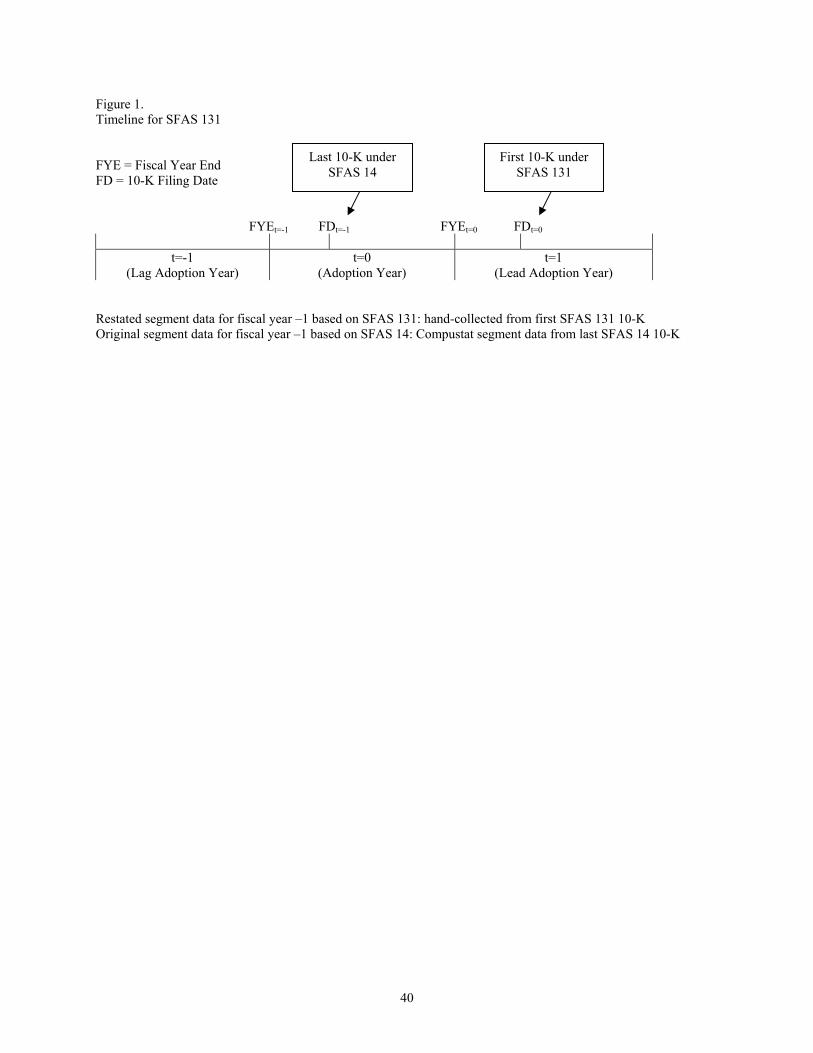
40

Figure 1. Timeline for SFAS 131 FYE = Fiscal Year End FD = 10-K Filing Date FYEt=-1 FDt=-1 FYEt=0 FDt=0

t=-1

(Lag Adoption Year) t=0

(Adoption Year) t=1

(Lead Adoption Year) Restated segment data for fiscal year –1 based on SFAS 131: hand-collected from first SFAS 131 10-K Original segment data for fiscal year –1 based on SFAS 14: Compustat segment data from last SFAS 14 10-K

First 10-K under SFAS 131

Last 10-K under SFAS 14

41

Table 1. Correlation Coefficients between Segments/Stand-Alone Firms and their Industries under SFAS14 and SFAS 131 Stand-Alone Firms (CorrFirm) Segments (CorrSegment)

Mean (t-statistics) SFAS 14 SFAS 131 Dif. SFAS 14 SFAS 131 Dif. Dif of Dif

Sales: Equal-Weighted

0.478***(15.16)

0.276***(4.60)

-0.201***(-2.82)

0.369***(10.98)

0.176***(3.95)

-0.193***(-3.47)

0.009 (0.14)

Value-Weighted

0.301***(5.77)

0.220***(3.36)

-0.082***(-1.11)

0.212***(4.81)

0.176***(3.78)

-0.036 (-0.65)

0.045 (0.73)

Earnings: Equal-Weighted

0.264***(7.98)

0.252***(4.71)

-0.012 (-0.19)

0.148***(4.79)

0.114***(3.00)

-0.034 (-0.67)

-0.022 (-0.39)

Value-Weighted

0.180***(4.47)

0.231***(4.06)

0.051 (0.79)

0.133***(4.81)

0.106***(3.08)

-0.027 (-0.63)

-0.078 (-1.28)

* , ** , *** Statistical significance at the 10%, 5%, and 1% level (two-tailed test). The t-statistics are reported in parentheses. CORRFirm Average correlation of sales (earnings) of stand-alone firms with their respective industries. CORRSegment Average correlation of sales (earnings) of segments (of multi-segment firms) with their respective

industries. In computing the industry indexes, we include in each industry all businesses that are either stand-alone companies or segments of multisegment firms. For each business, an industry index is formed by averaging (equally weighted or value-weighted by entity sales) the performance measure (i.e., sales or earnings) across all other entities in the industry.

42

Table 2. Descriptive Statistics: The Distribution of Single-Segment and Multisegment Firms under SFAS 14 & SFAS 131 for the Lag Adoption Year

Panel A. Full Sample

SFAS 131 Single-segment Multisegment Total no. of obs.

SFAS 14

Single-segment 1792 543 2335 (76.75%) (23.25%) (100%) [100.00%] [44.99%] [77.86%]

Multisegment 0 664 664 (0.00%) (100.00%) (100%) [0.00%] [55.01%] [22.14%]

Total no. of obs. 1792 1207 2999 (59.75%) (40.25%) [100%] [100%]

Panel B. SFAS 131 Multisegment Sample

Reporting Δ in Cumulative Cumulative # of Segments Frequency Percent Frequency Percent

-3 1 0.08 1 0.08 -2 4 0.33 5 0.41 -1 39 3.23 44 3.65 0 472 39.11 516 42.75

+1 357 29.58 873 72.33 +2 208 17.23 1081 89.56 +3 89 7.37 1170 96.93 +4 30 2.49 1200 99.42 +5 6 0.50 1206 99.92 +6 1 0.08 1207 100.00

Full Sample: The adoption year is the first fiscal year in which SFAS 131 was adopted and the lag adoption year is the preceding fiscal year. The SFAS 131 restated segment data for the lag adoption year are taken from the footnotes of the annual reports of the adoption year. Our original sample includes all firms listed in Compustat, CRSP and IBES with restated segment data available for the lag adoption year. The full sample is a subset of the original sample for which restatements of historical segment data are made only due to adoption of SFAS 131. See Section 4 for a more detailed discussion on the construction of the full sample. SFAS 131 Multisegment Sample: Firms within the full sample that are reported as multisegment firms in the restated segment footnotes for the lag adoption year.

43

Table 2. continued Panel C. SFAS 131 Multisegment: No-Change Sample

# of Segments Cumulative Cumulative (based on SFAS 131) Frequency Percent Frequency Percent

2 242 51.27 242 51.27 3 132 27.97 374 79.24 4 59 12.50 433 91.74 5 21 4.45 454 96.19 6 10 2.12 464 98.31 7 8 1.69 472 100.00

Panel D. SFAS 131 Multisegment: Aggregation Sample

# of Segments Cumulative Cumulative (based on SFAS 131) Frequency Percent Frequency Percent

2 259 37.48 259 37.48 3 232 33.57 491 71.06 4 127 18.38 618 89.44 5 53 7.67 671 97.11 6 16 2.32 687 99.42 7 3 0.43 690 99.86 9 1 0.14 691 100.00

Aggregation Sample: Firms within the SFAS 131 multisegment sample with the restated number of segments under SFAS 131 greater than the number reported in the original annual report under SFAS 14 in the lag adoption year. No-Change Sample: Firms within the SFAS 131 multisegment sample that had the same number of reported segments under both reporting regimes in the lag adoption year. Panel E. Pre- and Post-SFAS 131 Single Segment Industry Share (SS_INDSHR)1

Mean Median 1995 45% 43% 1996 47% 45% 1997 47% 43% 1998 32% 26% 1999 36% 27% 2000 33% 25%

1 Single segment industry share is the proportion of sales from single segment firms to total industry sales. Total industry sales include sales from single segment firms and segments of multisegment firms that are in Compustat. Industry is defined by 2-digit SIC code. The mean single segment industry share is computed as the average across all industries.

44

Table 3. Descriptive Statistics: Firm Characteristics of the Aggregation and No-Change Samples in the Pre-SFAS131 Period

Mean

Aggregation Sample

No-Change Sample

Dif. Bet.

Aggregation & No-Change Samples

Total Assets

1980.17

4152.96

-2172.79*** (-5.33)

Total Sales

1557.49

3103.91

-1546.42*** (-5.71)

Total Market Value of Equity (N=681;458)

1934.18

3447.15

-1512.97*** (-4.20)

Market-to-Book (MKT_BK) (N=668;446)

3.28

2.77

0.51*** (3.13)

Leverage (LEVERAGE)

0.20

0.20

0.00 (0.48)

Number of Segments (NUMSEG)

3.06

2.83

0.23*** (3.42)

Level of Disaggregation (DISAGG) (N=670;443)

0.60

0.21

0.40*** (10.96)

Level of Diversification (DIVERSIFICATION) (N=690;469)

0.59

0.57

0.02** (2.02)

Segment Industry Diversity (SEG_DIVERSITY)

0.62

0.76

-0.14*** (-9.49)

No. of Observations 691 472

* , ** , *** Statistical significance at the 10%, 5%, and 1% level (two-tailed test). The t-statistics are reported in parentheses. Aggregation Sample: Firms within the SFAS 131 multisegment sample with the restated number of segments under SFAS 131 greater than the number reported in the original annual report under SFAS 14 in the lag adoption year. No-Change Sample: Firms within the SFAS 131 multisegment sample that had the same number of reported segments under both reporting regimes in the lag adoption year. Variable Definitions: Except for NUMSEG, DIVERSIFICATION and SEG_DIVERSITY, all other variables are measured as the average over the three years prior to the adoption year. The adoption year is the first fiscal year in which SFAS 131 was adopted. MKT_BK The ratio of the market value of equity to book value of equity. LEVERAGE The ratio of long-term debt to total assets. NUMSEG

The number of segments reported in the restated segment footnotes based on SFAS 131 for the lag adoption year.

DISAGG

The natural log of

# of segments # of business activities , where

the number of business activities is measured as the number of different two-digit SIC codes the firm operates in during the segment report year, as collected from the Standard & Poor’s Register of Corporations, Directors and Executives.

DIVERSIFICATION

The revenue-based Herfindahl index measure of a firm’s diversification.

It is calculated as: ∑i=1

nSi

2 / ⎝⎜⎛

⎠⎟⎞

∑i=1

nSi

2

where n=number of segments; Si = segment i’s sales

SEG_DIVERSITY

The ratio of the number of unique primary SIC codes (from Compustat’s segment database) across segments to the total number of restated SFAS 131 segments.

45

Table 4. Univariate Analysis of Factors Associated with Segment Aggregation Under SFAS 14 Measures of abnormal profit, speed of abnormal profit adjustment and within-firm range of segment profits

Aggregation Sample

No-Change Sample

Mean Median

Difference

Mean

Median

Std Dev

Mean

Median

Std Dev Difference

(t-stat) (Wilcoxon

z-stat) Abnormal Profit: Industry adjusted ROA (ABN_PROFITROA) (N=617; 426)

0.071

0.041

0.137

0.035

0.018

0.119

0.036***(4.51)

0.023***(4.17)

Industry adjusted ROE (ABN_PROFITROE) (N=598; 412)

0.189

0.073

0.320

0.123

0.049

0.275

0.066***(3.52)

0.024***(3.01)

Speed of Abnormal Profit Adjustment: Weighted by Segment Sales (PROFIT_ADJSale) (N=590; 403)

0.783

0.767

0.404

0.723

0.739

0.340

0.060***(2.55)

0.028** (2.29)

Weighted by Segment Assets (PROFIT_ADJAsset) (N=382; 367)

0.802

0.767

0.402

0.743

0.738

0.334

0.059** (2.17)

0.029** (2.21)

Within Firm Heterogeneity in Segment Profits: Range of Segment ROA (RANGE_PROFITROA) (N=380; 366)

0.375

0.164

0.666

0.234

0.127

0.377

0.141***(3.12)

0.037***(3.09)

Range of Segment ROS (RANGE_ PROFITROS) (N=561; 401)

0.612

0.137

1.377

0.353

0.122

0.791

0.259***(3.03)

0.015** (2.18)

* , ** , *** Statistical significance at the 10%, 5%, and 1% level (two-tailed test). The t-statistics are reported in parentheses. Aggregation Sample: Firms within the SFAS 131 multisegment sample with the restated number of segments under SFAS 131 greater than the number reported in the original annual report under SFAS 14 in the lag adoption year. No-Change Sample: Firms within the SFAS 131 multisegment sample that had the same number of reported segments under both reporting regimes in the lag adoption year. Summary of Variable Definitions: ABN_PROFITROA/ROE

The average of industry-adjusted ROA or ROE (at the firm-level) over the three years prior to the adoption year. Industry is defined by the narrowest SIC code with at least five firms.

PROFIT_ADJSale/Asset An estimate of the speed of abnormal profit adjustment. RANGE_PROFITROA/ROS

The difference between the highest and lowest segment ROA or ROS, calculated using the restated SFAS 131 segment data for the lag adoption year.

46

Table 4. continued Construction of PROFIT_ADJ: 1) Compute each measure at the 2-digit SIC code level; 2) Match the industry measure to each segment by 2-digit SIC code; 3) Compute the firm-level measure by taking the average (weighted by segment sales or assets) of the corresponding segment measures. Industry Measure The persistence of abnormal profits for each industry is estimated using the following industry pooled cross-sectional time-series regression over the period 1985 to 1997:

Xijt = β0j + β1j (DnXijt-1) + β2j (DpXijt-1) + εijt where, Xijt = The year t difference between firm i’s ROA and mean ROA for its 2-digit industry, j. Dn = An indicator variable with the value of 1 if Xijt-1 is less than or equal to zero; 0 otherwise. Dp = An indicator variable with the value of 1 if Xijt-1 is greater zero; 0 otherwise. The coefficient estimate of DpXijt-1 (i.e., β2j) is used to measure the speed of adjustment for positive abnormal ROA in industry j (i.e., IPROFIT_ADJ). Firm-Level Measure After computing IPROFIT_ADJ at the 2-digit industry level, we match it to each segment (as restated under SFAS 131 for the lag adoption year) by industry and construct the corresponding firm-level measure in two ways:

i. Weighted by segment sales: PROFIT_ADJSale = ∑i=1

n [si/FS x IPROFIT_ADJSale i ]

ii. Weighted by segment assets: PROFIT_ADJAsset = ∑i=1

n [ai/FA x IPROFIT_ADJAsset i]

n = The number of segments based on the restated SFAS131 segment data for the lag adoption year si = Segment i’s sales based on the restated SFAS131 segment data for the lag adoption year ai = Segment i’s assets based on the restated SFAS131 segment data for the lag adoption year FS = Total firm sales FA = Total firm assets

47

Table 5. Probit and OLS Regression Analysis on the Determinants of Managers’ Decisions to Aggregate Segment Information Under SFAS 14 Panel A. Pearson/Spearman Correlation Matrix1

ABN_PROFIT PROFIT_ADJSale RANGE_PROFIT IND_AGG HERFSale SEG_DIVERSITY SIZE MKT_BK ABN_PROFIT 0.07 -0.07 0.05 0.00 -0.05 -0.17 0.42

0.03 0.03 0.07 0.96 0.07 0.00 0.00 983 952 1150 983 1152 1152 1105

PROFIT_ ADJSale 0.11 -0.07 -0.01 -0.22 0.00 -0.01 0.07 0.00 0.03 0.65 0.00 0.94 0.76 0.02 983 962 991 993 993 993 949

RANGE_ PROFIT -0.10 -0.04 0.08 -0.04 -0.11 0.05 0.01 0.00 0.24 0.01 0.23 0.00 0.16 0.79 952 962 960 962 962 962 919

IND_AGG 0.03 0.00 0.08 0.23 -0.05 -0.08 0.14 0.33 0.97 0.02 0.00 0.09 0.01 0.00 1150 991 960 991 1161 1161 1112

HERFSale -0.01 -0.13 -0.08 0.18 0.16 -0.15 0.00 0.64 0.00 0.02 0.00 0.00 0.00 0.94 983 993 962 991 993 993 949

SEG_DIVERSITY -0.08 -0.02 -0.08 -0.05 0.11 -0.05 -0.05 0.01 0.61 0.01 0.10 0.00 0.10 0.08 1152 993 962 1161 993 1163 1114

SIZE -0.11 -0.01 0.01 -0.10 -0.11 -0.06 -0.02 0.00 0.66 0.84 0.00 0.00 0.03 0.50 1152 993 962 1161 993 1163 1114

MKT_BK 0.29 0.07 0.05 0.08 -0.04 -0.12 -0.03 0.00 0.03 0.11 0.01 0.18 0.00 0.28 1105 949 919 1112 949 1114 1114

1 The correlation coefficients presented below (above) the diagonal are Pearson product moment (Spearman rank order) correlations. For each pair of variables, the first row reports the correlation coefficient, the second row the p-value, and the last row the number of observations.

48

Table 5. continued Panel B. Probit and OLS Regression Analysis (Dependent Variables: INC_NSEG and RPC_NSEG)

PROBIT:

INC_NSEG OLS:

RPC_NSEG

Coefficient (p-value) Marginal Effect

Coefficient (p-value)

INTERCEPT

1.449*** (0.00)

--

1.110*** (0.00)

ABN_PROFIT

0.949*** (0.01)

0.366

0.284** (0.01)

PROFIT_ADJ

0.248** (0.04)

0.096

0.063 (0.11)

RANGE_PROFIT

0.152*** (0.00)

0.059

0.045*** (0.00)

IND_AGG

0.653** (0.04)

0.252

0.357*** (0.00)

HERF

0.364 (0.63)

0.140

0.154 (0.55)

SEG_DIVERSITY

-1.285*** (0.00)

-0.496

-0.679*** (0.00)

SIZE

-0.125*** (0.00)

-0.048

-0.050*** (0.00)

MKT_BK

0.015 (0.39)

0.006

0.006 (0.30)

No. of Obs.:

Aggregation 535 535 No-Change 374 374 Total 919 919 Pseudo R2 (Probit) and Adj R2 (OLS) 0.13 0.21 * , ** , *** Statistical significance at the 10%, 5%, and 1% level (two-tailed test). The p-values are reported in parentheses. Aggregation Sample: Firms within the SFAS 131 multisegment sample with the restated number of segments under SFAS 131 greater than the number reported in the original annual report under SFAS 14 in the lag adoption year. No-Change Sample: Firms within the SFAS 131 multisegment sample that had the same number of reported segments under both reporting regimes in the lag adoption year. Dependent Variable: Probit Regression INC_NSEG

An indicator variable with the value of 1 for the aggregation sample; 0 for the no-change sample.

OLS Regression RPC_NSEG

The difference between the log of the number of segments reported under SFAS 14 (historical segment data) and SFAS 131 (restated segment data) for the lag adoption year.

Independent Variables: ABN_PROFIT

The average of industry-adjusted ROA (at the firm-level) over the three years prior to the adoption year. Industry is defined by the narrowest SIC code with at least five firms.

PROFIT_ADJ

An estimate of the speed of abnormal profit (positive abnormal ROA) adjustment that is constructed based on the weighted average of segment sales. See variable definitions in Table 3.

RANGE_PROFIT An estimate of within-firm heterogeneity in segment profits. IND_AGG

The level of pre-SFAS 131 industry aggregation. See section 5.1 for the construction of this variable. HERF

The Herfindahl index of 2-digit industry concentration constructed based on the weighted average of segment sales. SEG_DIVERSITY

Segment industry diversity, measured by the ratio of the number of unique SIC codes across segments to the total number of restated SFAS 131 segments.

SIZE The average of the log of the total assets over the three years prior to the adoption year. MKT_BK

The average ratio of the market value of equity to book value of equity over the three years prior to the adoption year.

The marginal effects measure the change in the probability of the firm increasing its number of reported segments upon adopting SFAS 131, given a one-unit change in the independent variables (xi). They are calculated as ф(βx)βi, where ф is the standard normal density and βi is the coefficient estimate of xi. The marginal effects are calculated at the means of the independent variables. The Pseudo R2 is computed as: 1 – exp[-2(ln Lr – ln L)/no. of obs.], where Lr and L are the log-likelihood functions evaluated at the restricted (slopes=0) and unrestricted estimates, respectively.

49

Table 6. The Relation Between Segment Aggregation under SFAS 14 and Abnormal Profitability Panel A. Univariate Analysis of Change in Firm-Level Abnormal Profitability: Before and After SFAS 131

Pre-131

Post-131

Mean Median

Difference1

Mean

Median

Std Dev

Mean

Median

Std Dev Difference

(t-stat) (Wilcoxon

z-stat) Industry-Adjusted ROA (ABN_PROFITROA): Aggregation Sample (N=617)

0.071

0.041

0.137

0.055

0.022

0.136

-0.016***(-3.19)

-0.019** (-2.52)

No-Change (MS) Sample (N=426)

0.035

0.018

0.119

0.038

0.016

0.115

0.003 (0.67)

-0.002 (-0.02)

Difference bet. Aggregation and No-Change Samples

0.036***(4.51)

0.023***(4.17)

0.017** (2.21)

0.006* (1.74)

-0.019***(-2.78)

-0.017 (-1.58)

No-Change Single Segment Sample (N=1562)

0.073

0.048

0.229

0.078

0.049

0.161

0.005 (0.85)

0.000 (0.77)

Industry-Adjusted ROE (ABN_PROFITROE): Aggregation Sample (N=598)

0.189

0.073

0.320

0.128

0.075

0.259

-0.062***(-4.96)

0.002** (-2.28)

No-Change (MS) Sample (N=412)

0.123

0.049

0.275

0.091

0.047

0.234

-0.032** (-2.35)

-0.002 (-0.97)

Difference bet. Aggregation and No-Change Samples

0.066***(3.52)

0.024***(3.01)

0.036** (2.31)

0.028** (2.04)

-0.030 (-1.63)

0.004 (-0.99)

No-Change Single Segment Sample (N=1442)

0.261

0.106

0.49

0.118

0.066

0.29

-0.143***(11.25)

-0.031***(-3.05)

* , ** , *** Statistical significance at the 10%, 5%, and 1% level (two-tailed test). The t-statistics are reported in parentheses. ABN_PROFITROA/ROE

Pre-131: The average industry-adjusted return on assets (return on equity) over the three years prior to the adoption year. Post-131: The average industry-adjusted return on assets (return on equity) over the three years after the adoption year.

Aggregation Sample: Firms within the SFAS 131 multisegment sample with the restated number of segments under SFAS 131 greater than the number reported in the original annual report under SFAS 14 in the lag adoption year. No-Change Sample: Firms within the SFAS 131 multisegment sample that had the same number of reported segments under both reporting regimes in the lag adoption year. 1 Because the Wilcoxan two-sample test is based on signed-ranks, the test results are not always consistent with the direction of the difference across the medians.

50

Table 6 continued Panel B. Two Stage Least Squares and OLS Regression Analysis of Change in Firm-Level Abnormal Profitability

Two Stage Least Squares Estimation (Second Stage) OLS Estimation

∆ABN_PROFIT

(ROA)

∆ABN_PROFIT (ROE)

∆ABN_PROFIT (ROA)

∆ABN_PROFIT (ROE)

Model 1 Model 2 Model 3 Model 4 Model 1 Model 2 Model 3 Model 4

INTERCEPT

-0.022 (0.37)

-0.048** (0.02)

-0.199***(0.00)

-0.229***(0.00)

-0.056***(0.00)

-0.060***(0.00)

-0.229***(0.00)

-0.221***(0.00)

P_INC_NSEG (from 1st stage Probit )

-0.056** (0.03)

--

-0.031 (0.65)

--

--

--

--

--

P_RPC_NSEG (from 1st stage OLS)

--

-0.023 (0.22)

--

0.011 (0.83)

--

--

--

--

INC_NSEG

--

--

--

--

-0.009 (0.25)

--

0.012 (0.57)

--

RPC_NSEG

--

--

--

--

--

-0.003 (0.69)

--

-0.001 (0.96)

PROFIT_ADJ

0.017 (0.10)

0.013 (0.20)

0.040 (0.14)

0.036 (0.17)

0.012 (0.25)

0.011 (0.28)

0.033 (0.21)

0.034 (0.19)

SIZE

0.007*** (0.00)

0.008***(0.00)

0.029***(0.00)

0.031***(0.00)

0.008***(0.00)

0.009***(0.00)

0.031***(0.00)

0.030***(0.00)

MKTBK

-0.002 (0.15)

-0.002* (0.09)

-0.014***(0.00)

-0.014***(0.00)

-0.003* (0.06)

-0.003* (0.06)

-0.014***(0.00)

-0.014***(0.00)

No. of firm Obs. (pre & post periods)

829 (1658)

829 (1658)

829 (1658)

829 (1658)

831 (1662)

831 (1662)

820 (1640)

820 (1640)

Adjusted R2 0.03 0.03 0.05 0.05 0.03 0.03 0.05 0.05

* , ** , *** Statistical significance at the 10%, 5%, and 1% level (two-tailed test). The p values are reported in parentheses.

51

Table 6. continued

We estimate the abnormal profit regressions with two stage least squares using the fitted values from the following probit (for models 1 and 2) and OLS (for models 3 and 4) first stage regression models as the instrumental variables: Probit: INC_NSEC = α + β1 ABN_PROFIT + β2 PROFIT_ADJ + β3 RANGE_PROFIT + β4 HERF + β5 SEG_DIVERSITY + β6 SIZE + β7 MKT_BK + ε,

where INC_NSEG is defined below (see table 5 for a summary of the variable definitions for the probit model). The results of the first stage probit regression are reported in panel B of table 5.

OLS: RPC_NSEG = α + β1 ABN_PROFIT + β2 PROFIT_ADJ + β3 RANGE_PROFIT + β4 HERF + β5 SEG_DIVERSITY + β6 SIZE + β7 MKT_BK + ε,

where RPC_NSEG is defined below (see table 5 for a summary of the variable definitions for the OLS model). The results of the first stage OLS regression are reported in panel B of table 5.

Dependent Variables: ∆ABN_PROFITROA/ROE

The difference between pre-131 and post-131 abnormal profits, which are defined as follows: Pre-131: The average industry-adjusted return on assets (return on equity) over the three years prior to the adoption year. Post-131: The average industry-adjusted return on assets (return on equity) over the three years after the adoption year.

Independent Variables: P_INC_NSEG The fitted probabilities from the first stage probit regression model. P_RPC_NSEG The predicted values from the first stage OLS regression model. INC_NSEG An indicator variable with the value of 1 for the increase disaggregation sample; 0 for the no-change sample. RPC_NSEG

The difference between the log of the number of segments reported under SFAS 14 (historical segment data) and SFAS 13 (restated segment data) for the lag adoption year.

PROFIT_ADJ

An estimate of the speed of abnormal profit (positive abnormal ROA) adjustment that is constructed based on the weighted average of segment sales. See the variable definition in Table 4.

SIZE The average of the log of the total assets over the same period for which ABN_PROFIT is calculated. MKTBK The average ratio of the market value of equity to book value of equity over the same period for which ABN_PROFIT is calculated.

52

Table 7. Univariate and Multivariate (Probit and OLS) Regression Analysis on the Determinants of Managers’ Decisions to Aggregate Segment Information Under SFAS 14: Additional Analysis on Measures of Agency Costs Panel A. Univariate Analysis

Aggregation Sample

No-Change Sample

Mean Median

Difference

Mean

Median

Std Dev

Mean

Median

Std Dev Difference

(t-stat) (Wilcoxon

z-stat) Number of loss segments (NLOSSSEG) (N=658; 466)

0.544

0.000

0.799

0.382

0.000

0.669

0.162***(3.69)

--

Proportion of firms with at least 1 loss segment (D_LOSSSEG) (N=658; 466)

0.403

0.000

0.491

0.294

0.000

0.456

0.109***(3.82)

--

Excess capital expenditures (TRANSFER) (N=446; 407)

3.899

0.000

13.848

3.579

0.000

9.731

0.320 (0.39)

--

Proportion of firms with excess capital expenditures (D_TRANSFER) (N=446; 407)

0.460

0.000

0.499

0.420

0.000

0.494

0.040 (1.16)

--

Within firm heterogeneity in segment PE (RANGE_PE) (N=498; 429)

8.21

6.41

6.54

7.46

5.74

6.33

0.75* (1.77)

0.67** (2.06)

* , ** , *** Statistical significance at the 10%, 5%, and 1% level (two-tailed test). The t-statistics are reported in parentheses. Aggregation Sample: Firms within the SFAS 131 multisegment sample with the restated number of segments under SFAS 131 greater than the number reported in the original annual report under SFAS 14 in the lag adoption year. No-Change Sample: Firms within the SFAS 131 multisegment sample that had the same number of reported segments under both reporting regimes in the lag adoption year. Summary of Variable Definitions: NLOSSSEG The number of segments with losses. D_LOSSSEG An indicator variable with the value of 1 for firms with at least one loss segment; 0 otherwise. TRANSFER

Max ⎣⎡ ⎦⎤

Sum of segment Excess CAPX - Firm level Excess CAPX Mtk value of Equity , 0 x 100, where

Excess CAPX = max [CAPX – (OPS+DEP), 0] CAPX = capital expenditures OPS = operating profits DEP = depreciation expense

D_TRANSFER An indicator variable with the value of 1 if TRANSFER is greater than 0; 0 otherwise. RANGE_PE A measure of within firm heterogeneity in segment PE. See section 5.3 for the construction of this variable.

53

Table 7 continued Panel B. Pearson/Spearman Correlation Matrix1

D_LOSSSEG D_TRANSFER RANGE_PE ABN_PROFIT PROFIT_ADJ

RANGE_ PROFIT IND_AGG HERF

SEG_ DIVERSITY SIZE MKT_BK

D_LOSSSEG 1.00 0.50 0.06 -0.17 -0.02 0.31 0.04 -0.01 -0.12 -0.02 -0.04 0.00 0.04 0.00 0.59 0.00 0.19 0.69 0.00 0.41 0.16 852 1124 1113 958 958 1122 958 1124 1124 1076

D_TRANSFER 1.00 0.06 -0.09 -0.06 0.17 0.01 0.01 -0.08 0.13 -0.09 0.06 0.01 0.14 0.00 0.70 0.77 0.02 0.00 0.01 853 851 731 731 852 731 853 853 830

RANGE_PE 1.00 -0.03 -0.03 0.11 0.09 0.14 0.24 0.13 0.03 0.24 0.37 0.00 0.00 0.00 0.00 0.00 0.36 1152 993 962 1161 993 1163 1163 1114

D_LOSSSEG 1.00 0.50 0.05 -0.16 -0.03 0.49 0.05 -0.02 -0.12 -0.03 -0.10 0.00 0.12 0.00 0.29 0.00 0.08 0.62 0.00 0.29 0.00 852 1124 1113 958 958 1122 958 1124 1124 1076

D_TRANSFER 1.00 0.08 -0.08 -0.08 0.29 0.01 0.02 -0.07 0.13 -0.12 0.03 0.02 0.03 0.00 0.81 0.56 0.03 0.00 0.00 853 851 731 731 852 731 853 853 830

RANGE_PE 1.00 -0.06 -0.01 0.18 0.05 0.10 0.38 0.16 0.06 0.06 0.64 0.00 0.09 0.00 0.00 0.00 0.07 1152 993 962 1161 993 1163 1163 1114

1 The correlation coefficients presented in the top two panels (bottom tow panels) are Pearson product moment (Spearman rank order) correlations. For each pair of variables, the first row reports the correlation coefficient, the second row the p-value, and the last row the number of observations.

54

Table 7 continued Panel C. Multivariate Probit Analysis (Dependent Variables: INC_NSEG)

Model 1 Model 2 Model 3 Model 4

Coefficient (p-value)

Marginal Effect

Coefficient (p-value)

Marginal Effect

Coefficient (p-value)

Marginal Effect

Coefficient (p-value)

Marginal Effect

INTERCEPT

1.339*** (0.00)

--

1.061***(0.00)

--

0.840***(0.01)

--

0.515 (0.15)

--

ABN_PROFIT

1.091*** (0.00)

0.420

0.806** (0.04)

0.321

0.790** (0.04)

0.313

0.444 (0.29)

0.177

PROFIT_ADJ

0.244** (0.04)

0.094

0.301** (0.03)

0.120

0.286** (0.04)

0.113

0.328** (0.04)

0.131

RANGE_PROFIT

0.121*** (0.01)

0.047

0.149***(0.00)

0.059

0.136***(0.01)

0.054

0.171*** (0.00)

0.068

D_LOSSSEG

0.222** (0.03)

0.086

--

--

0.237** (0.03)

0.094

--

--

D_TRANSFER

--

--

0.124 (0.22)

0.049

--

--

0.121 (0.28)

0.048

RANGE_PE

--

--

--

--

0.003 (0.70)

0.001

-0.000 (0.96)

0.000

IND_AGG

0.638** (0.05)

0.246

0.454 (0.22)

0.181

0.756** (0.04)

0.300

0.679 (0.11)

0.270

HERF

0.292 (0.70)

0.112

0.612 (0.49)

0.243

0.491 (0.57)

0.195

0.643 (0.52)

0.256

SEG_DIVERSITY

-1.241*** (0.00)

-0.478

-1.265***(0.00)

-0.503

-0.929***(0.00)

-0.368

-0.909*** (0.00)

-0.362

SIZE

-0.123*** (0.00)

-0.047

-0.093***(0.00)

-0.037

-0.099***(0.00)

-0.039

-0.066** (0.03)

-0.026

MKT_BK

0.016 (0.35)

0.006

0.003 (0.90)

0.001

0.012 (0.53)

0.005

0.006 (0.80)

0.002

No. of Obs.:

Aggregation 534 371 388 276 No-Change 371 336 334 303 Total 905 707 722 579 Pseudo R2 0.13 0.11 0.10 0.08

* , ** , *** Statistical significance at the 10%, 5%, and 1% level (two-tailed test). The p values are reported in parentheses. See tables 5B and 7A for variable definitions. The marginal effects measure the change in the probability of the firm increasing its number of reported segments upon adopting SFAS 131, given a one-unit change in the independent variables (xi). They are calculated as ф(βx)βi, where ф is the standard normal density and βi is the coefficient estimate of xi. The marginal effects are calculated at the means of the independent variables. The Pseudo R2 is computed as: 1 – exp[-2(ln Lr – ln L)/no. of obs.], where Lr and L are the log-likelihood functions evaluated at the restricted (slopes=0) and unrestricted estimates, respectively.

55

Table 7 continued Panel D. Multivariate OLS Analysis (Dependent Variables: RPC_NSEG)

Model 1 Model 2 Model 3 Model 4

Coefficient (p-value)

Coefficient (p-value)

Coefficient (p-value)

Coefficient (p-value)

INTERCEPT

1.037*** (0.00)

0.922*** (0.00)

0.963*** (0.00)

0.754*** (0.00)

ABN_PROFIT

0.366*** (0.00)

0.294** (0.02)

0.380*** (0.00)

0.248* (0.08)

PROFIT_ADJ

0.060 (0.13)

0.095** (0.04)

0.078* (0.10)

0.109** (0.05)

RANGE_PROFIT

0.028** (0.03)

0.029** (0.04)

0.029** (0.05)

0.030* (0.05)

D_LOSSSEG

0.137*** (0.00)

--

0.137*** (0.00)

--

D_TRANSFER

--

0.083** (0.02)

--

0.081** (0.03)

RANGE_PE

--

--

0.004 (0.17)

0.002 (0.57)

IND_AGG

0.347*** (0.00)

0.396*** (0.00)

0.430*** (0.00)

0.496*** (0.00)

HERF

0.125 (0.63)

0.210 (0.48)

0.125 (0.68)

0.203 (0.56)

SEG_DIVERSITY

-0.648*** (0.00)

-0.627*** (0.00)

-0.594*** (0.00)

-0.506*** (0.00)

SIZE

-0.048*** (0.00)

-0.043*** (0.00)

-0.050*** (0.00)

-0.038*** (0.00)

MKT_BK

0.006 (0.24)

0.004 (0.53)

0.004 (0.54)

0.006 (0.44)

No. of Obs.:

Aggregation 534 371 388 276 No-Change 371 336 334 303 Total 905 707 722 579 Adjusted R2 0.22 0.18 0.19 0.13 * , ** , *** Statistical significance at the 10%, 5%, and 1% level (two-tailed test). The p values are reported in parentheses. See tables 5B and 7A for variable definitions.