Segment Profitability and the Proprietary and Agency Costs of Disclosure*

Philip G. Berger Graduate School of Business, University of Chicago, 1101 E. 58th St., Chicago, IL 60637

and

Rebecca N. Hann

Leventhal School of Accounting, University of Southern California, Los Angeles, CA 90089

August, 2005

* This paper was previously circulated under the title “Segment Profitability and the Proprietary Costs of Disclosure.” We thank Melissa Boyle and Todd Yuba for their research assistance and two anonymous referees for many helpful comments. We have also benefited from the comments of Ray Ball, Anne Beatty, Bob Bowen, Ted Goodman, Il-Horn Hann, Ole-Kristian Hope, Bjorn Jorgensen, Christian Leuz, Ron Lott, Steve Monahan, Maria Ogneva, Joe Piotroski, Gord Richardson, Tjomme Rusticus, Terry Shevlin, Suraj Srinivasan, Ram Venkataraman, Joe Weber, and workshop participants at the following universities and conferences: University of Arizona, Canadian Academic Accounting Association's Ph.D. Consortium, University of Chicago, Columbia University's Burton Workshop Conference, Emory University, University of Illinois (Chicago), London Business School, University of Minnesota Empirical Accounting Conference, NYU Accounting Summer Camp, Rutgers University, Stanford University Accounting Summer Camp, University of Toronto, and University of Washington. Berger gratefully acknowledges financial support from the Neubauer Family Faculty Fellows program at the University of Chicago Graduate School of Business.

Segment Profitability and the Proprietary and Agency Costs of Disclosure

Abstract:

We exploit the recent change in segment reporting rules (from SFAS 14 to SFAS 131) to examine

two motives for managers to conceal segment information: proprietary costs and agency costs. By

comparing a hand-collected sample of restated SFAS 131 segments with the historical SFAS 14

segments, we are able to identify the “new” segments that were previously aggregated under the old

standard. This unique setting allows us to examine at the segment-level whether managers’ decisions to

aggregate segment information are driven by proprietary cost as well as agency cost motives. To

disentangle these two motives, we split our sample into four partitions based on our measures of agency

and proprietary costs. We find that firms with relatively high agency costs and relative low proprietary

costs tend to aggregate segments that have worse abnormal profits. This result is consistent with

entrenched managers using their discretion opportunistically to conceal negative information under the

old standard. On the other hand, firms with relatively high proprietary costs and relatively low agency

costs are more likely to aggregate segments that have higher abnormal profits, suggesting that managers

withhold segment information when proprietary cost motive dominates. Overall, we find that segment

profitability is an important determinant of managers’ segment reporting decisions. Our results suggest

that managers’ decisions to aggregate segment information are driven not only by the proprietary cost

motive, but also the agency cost motive.

Keywords: segment profitability; segment reporting; discretionary disclosure; proprietary costs; agency costs Data Availability: All data are available from public sources, except for the restated SFAS 131 segment data, which are proprietary.

1

1. Introduction

This paper exploits the recent change in U.S. segment reporting rules to examine two motives for

managers to conceal segment information: proprietary costs and agency costs. Prior studies (e.g., Harris

[1998]; Ettredge, Kwon, and Smith [2002]; Piotroski [2003]) have focused primarily on examining the

proprietary costs of segment disclosure, probably because managers often express concerns that more

segment disclosure would force them to provide valuable proprietary information to competitors.1

Managers, however, may also have incentives to aggregate segment data to obscure details about their

firms’ underlying agency problems. Segment data are of particular importance for revealing agency

concerns because they provide information about a company’s diversification strategy and transfers of

resources across segments. In this study, we examine whether managers’ decisions to aggregate segment

information are driven by proprietary cost as well as agency cost motives.

The recent mandated segment reporting change offers a unique setting to address this question.2

Under the old standard, SFAS 14, companies were required to classify line-of-business (LOB) segment

information using the industry approach. A major concern with SFAS 14 was that discretion in the

definition of “industry” allowed managers to report more aggregated segment information to external

users than what was reported internally (Ernst & Young [1998]). The new standard, SFAS 131, on the

other hand, follows a management approach, where segments are presented based on how management

internally evaluates the operating performance of its business units.3 Recent studies (e.g., Street, Nichols,

and Gray [2000]; Herrmann and Thomas [2000]; Berger and Hann [2003]) document that the number of

reporting segments under SFAS 131 increased significantly relative to SFAS 14. One interpretation of

this finding, and a maintained assumption of this study, is that the new standard offers relatively less

discretion for segment aggregation. Based on this assumption, we examine whether managers use the

1 For instance, Ettredge et. al (2002) report that 86% of the industrial firms that commented on the exposure draft for SFAS 131 opposed the new standard on the grounds that “it would put them at competitive disadvantage.” 2 SFAS 14 is FASB Statement No. 14, Financial Reporting for Segment of a Business Enterprise (FASB 1976). SFAS 131 is FASB Statement No. 131, Disclosures about Segments of an Enterprise and Related Information (FASB 1997). 3 See Berger and Hann (2003) for a more detailed discussion on the main differences between SFAS 14 and SFAS 131.

2

discretion afforded under SFAS 14 to conceal segment information because of proprietary and agency

costs.

Using a hand-collected database that contains restated SFAS 131 segment data, we compare the

segment information generated under the two reporting regimes for the same firm at the same point in

time. The restated data allow us to identify the “new” SFAS 131 segments that were previously

aggregated under the old standard and hence examine managers’ reporting choice at the segment-level.

Another advantage of this mandated setting is that it allows us to identify a sample of firms where the

costs of expanding disclosure likely outweigh the benefits. On one hand, expanded disclosure about

segment profitability may provide valuable information to the capital markets (hereafter, capital market

benefits). On the other hand, there are potential data collection costs as well as proprietary and agency

costs associated with greater segment disclosure. Therefore, it is in general difficult to have an

unambiguous prediction on the impact of segment profitability on managers’ reporting choices, which is a

common difficulty that prior studies on voluntary segment disclosure face (e.g., Harris [1998] and

Piotroski [2003]). In our setting, the segment data required under the new standard were presumably

already available internally, so there are probably few, if any, data collection costs necessary to provide

more segment information. Intuitively, if the capital market benefits outweigh other costs, firms could

have voluntarily disclosed more disaggregated information under the old standard. Put differently, the

aggregation of segments under the old reporting regime likely reflects a net cost (either proprietary and/or

agency related) of more disaggregated disclosure.

In this study, we focus on abnormal segment profits as the primary determinant of managers’ segment

reporting choices and examine whether segment profitability is related to both proprietary and agency

costs of segment disclosure. From the proprietary cost perspective, it is important to identify what

proprietary information is being revealed in segment footnotes that would otherwise be unknown (or

unlikely to be known) to competitors. Given the limited set of items that are disclosed in segment

footnotes, segment profitability is likely the most valuable piece of information that managers would like

to withhold from competitors. In other words, information about how well the segment performs relative

3

to its industry peers likely constitutes valuable proprietary information. Our first hypothesis predicts that

managers are more likely to aggregate the segments with relatively high abnormal profits when

proprietary costs are the primary motive.

Regarding the agency cost motive, we argue that entrenched managers may aggregate segment data to

avoid revealing underlying agency problems associated with suboptimal cross-segment transfer of

resources. Prior studies find evidence consistent with internal capital markets in conglomerates

transferring funds across segments in a suboptimal manner (e.g., Berger and Ofek [1995]; Lamont [1997];

Shin and Stulz [1998]; Rajan, Servaes and Zingales [2000]). Managers of firms with these agency

problems may try to hide the segments that tend to have relatively poor profits. We therefore predict that

managers are more likely to aggregate the segments with relatively low abnormal profits if agency costs

are the dominating motive.

We test the proprietary and agency cost hypotheses by examining abnormal segment profits, proxied

by industry-adjusted returns on sales, across the “new” and the “old” SFAS 131 segments, which reflects

managers’ discretionary reporting decisions under the old standard. The new segments are segments that

were previously aggregated under the old regime, presumably because of the relatively greater discretion

afforded under SFAS 14. The old segments are those that were already reported as a separate line-of-

business segments under the old standard. To disentangle the agency cost (AC) motive from the

proprietary cost (PC) motive, we partition our sample such that one cost consideration is likely to

dominate the other. Specifically, we argue that proprietary costs are unlikely an important factor in the

aggregation decision if none of the firm’s segments earns an abnormal profit relative to its industry peers.

We therefore assume that the firms with at least one segment making a positive abnormal profit are likely

to have relatively high proprietary costs (hereafter, “high PC” subsample). All other firms in the sample

are included in the “low PC” subsample. From the agency cost perspective, we assume that the firms

with excessive cross-segment transfers are likely to experience relatively higher agency costs; we

therefore classify these firms in the “high AC” group. The firms without substantial cross-segment

transfers are included in the “low AC” subsample. These two classifications based on agency and

4

proprietary costs yield four partitions. We focus on the following two partitions in our hypothesis testing:

1) high PC and low AC (where PC motive likely dominates); and 2) High AC and low PC (where AC

motive likely dominates).

Using a probit regression analysis on managers’ reporting decisions, we find evidence supporting

both the proprietary and agency cost hypotheses. In particular, for the subsample of firms with relatively

high agency costs, we find that the new segments tend to have worse abnormal profits. This result is

consistent with entrenched managers hiding the poorly performing segments under the old standard when

the agency cost motive dominates. On the other hand, for the subsample of firms with relatively high

proprietary costs, the new segments are associated with higher profits than their industry peers,

suggesting that managers avoid revealing profitable segment information when proprietary costs are the

primary motive. Interestingly, we find that for the subsample where both agency and proprietary cost

motives are present (i.e., the high AC and high PC partition), the agency cost motive appears to dominate.

In particular, the new segments in this subsample are associated with lower abnormal profits, suggesting

that managers, when faced with both agency and proprietary cost incentives, may place more weight on

the agency costs.

Given these results, we then examine whether the new segments experience a greater decline in

abnormal profits than the old segments after the adoption of SFAS 131 for the subset of firms where the

proprietary cost motive dominates. Of the four partitions (based on AC and PC) in our sample, we find

that the change in abnormal segment profits is more negative for the new segments than for the old

segments only in the subsample where proprietary costs dominate (i.e., high PC and low AC partition).

For the rest of the three partitions, the change in abnormal profits is insignificantly different across the

new and the old segments. These results are consistent with managers’ concern about competitive harm

from the new reporting standard.

Our results contribute to the literature on the following three dimensions. First, the hand-collected

restated SFAS 131 segment data allows us to study managers’ reporting decisions at the segment-level,

which is an important improvement from prior studies that focus on firm-level analysis (e.g., Piotroski

5

[2003]; Botosan and Stanford [2005]). This is important both conceptually and methodologically because

it is segment profits, not firm-level profits that managers try to conceal, regardless of whether managers

are motivated by proprietary or agency cost motives. To our knowledge, Harris (1998) is the only other

study that examines managers’ segment reporting decisions at the segment level. Her study focuses on

measures that capture how profitable or competitive the segment’s industry is, which are likely of second

order effect because industry-wide data are generally already known to investors and competitors. Our

study focuses on how profitable the segment is relative to its industry, which is a more direct measure of

segment profits and hence a better proxy for proprietary costs of segment disclosure.

Second, as noted earlier, prior research (e.g., Harris [1998]; Ettredge et. al [2002]; Piotroski [2003])

focuses on examining the proprietary costs of disclosure. We extend these studies by incorporating the

agency costs of disclosure in our analysis. Two recent papers (Berger and Hann [2003]; Sanzhar [2003])

also address the agency costs of segment disclosure in their analyses. These studies focus on the impact

of more disaggregated segment disclosure under SFAS 131. They show that switching from reporting a

single segment under SFAS 14 to reporting multiple segments under SFAS 131 creates a diversification

discount, which is consistent with managers concealing information about agency costs under the old

standard. Their findings suggest that the agency cost motive may affect managers’ segment reporting

decisions. Our study complements theirs by providing more direct evidence that managers aggregate

poorly performing segments to hide their underlying agency problems.

Finally, as discussed before, prior studies on voluntary segment disclosure face the difficulty of

disentangling the capital market benefits and the proprietary costs of expanded segment disclosure. The

mandated setting used in this study allows us to largely overcome this difficulty that can result in

ambiguous predictions. A recent study by Berger and Hann (2003) and a concurrent study by Botosan

and Stanford (2005) use a similar mandated setting. Berger and Hann (2003) focus on examining whether

the more disaggregated segment information under the new standard provides new information to analysts

and investors. Their study does not examine managers’ reporting choices. Similar to our study, Botosan

and Stanford (2005) examine managers’ motives to withhold segment disclosure; however, our research

6

design and results differ in the following ways. While we examine managers’ reporting decisions at the

segment level and find evidence consistent with managers hiding poorly performing segments when the

agency cost motive dominates, they analyze profits at the firm-level and do not find evidence that

managers aggregate segments to conceal poor performance. As noted earlier, we believe it is segment

profits, not firm-level profits that managers try to conceal. Our study hence provides additional insight on

managers’ reporting choices beyond the inferences available from firm-level analysis.

Our analysis is subject to the following caveats. First, there are two maintained assumptions in this

study: 1) managers have relatively less discretion about the extent of segment aggregation under the new

standard;4 2) the increased disaggregation under the new standard reflects discretionary aggregation under

the old standard. To the extent they are not true, our inferences will be affected. Critics of the new

standard argue that managers may continue to have substantial discretion under SFAS 131 because firms

can presumably restructure their “internal operating segments” to avoid reporting more disaggregated

data. If this is true, the firms with opportunistic motives to conceal segment information would likely

continue to aggregate under the new regime. That means, either we would not find a significant increase

segment disclosure under the new standard, or that the increased reporting may not fully reflect

discretionary aggregation under the old standard. We acknowledge that this can be the case. However,

we offer the following arguments to support our assumptions.

First, Street et. al (2000) do not find any evidence of internal restructuring after SFAS 131.

Specifically, only six of the 160 firms in their sample realign their organizational structure after SFAS

131. This result suggests that while it is feasible to reorganize internally to withhold segment

information, few companies appear to utilize this flexibility under the management approach. Second, the

new standard was largely the result of extensive lobbying by analysts. From our conversations with the

4 We emphasize that our maintained assumption is that there is less discretion under SFAS 131 about the extent of segment aggregation. We recognize that the new standard can still have substantial discretion on some aspects of segment reporting under the new regime compared to the old standard, but probably not about the extent of segment aggregation (e.g., under SFAS 14, there were more specified the line items that must be reported about each segment).

7

FASB project manager on the new standard, it appears that one of the main concerns with analysts was

that “the old standard seems to offer unlimited discretion,” primarily because of the ample flexibility

inherent in the definitions of what an industry segment is.5 Further, under the old approach, segment

information was not subject to internal controls. The management approach under the new standard at

least ensures that the information was subject to internal controls. Analysts also seem to believe that it is

more difficult for firms to change its internal organization because there would be substantial

consequences to the change. Similarly, our conversations with auditors suggest that it is in general very

costly for companies to change their internal organization for external reporting purposes. Overall, it

appears that both analysts and auditors believe that the old standard afforded ample flexibility to

aggregate segment data. While the new standard does not completely preclude managers from

discretionary aggregation, it is arguably subject to less discretion on segment aggregation compared to the

old standard.

Several recent studies (Street et al. [2000]; Herrmann and Thomas [2000]; Berger and Hann [2003])

document that the number of reporting segments under SFAS 131 increased significantly relative to

SFAS 14. More importantly, the reporting change is overwhelmingly one-sided, with very few firms

decreasing the number of reported segments. In other words, there is at least descriptive evidence to

support that there was a significant increase in segment disaggregation. We acknowledge that the

documented increase in segment reporting under SFAS 131 could merely indicate a neutral application of

the new standard, i.e., the internal organization generally presents a finer partition than the industry

approach under the old standard and therefore firms report more disaggregated segments simply to

comply in good faith. To the extent this is true, our results will be affected. However, if the reporting

5 This quote is taken from an email correspondence with Ron Lott, who is one of the segment project managers at FASB who was involved in the proliferation of SFAS 131.

8

change indeed reflects only managers’ neutral compliance with the two reporting standards, it should

work against finding the hypothesized results.6

Finally, another maintained assumption of this study is that the new SFAS 131 segment data

constitute new public disclosures. A potential concern is that some of the information may already be

disclosed in the Management Discussion and Analysis (MD&A) section. Detailed examination of the

MD&A for a subsample of 100 firms with the greatest increase in the number of reporting segments

shows that MD&A contains little of the SFAS 131 segment earnings information (see Section 3.2.2 for a

detailed discussion). We also recognize that firms have incentives to obtain data from competitors and

can use non-public information to do so. However, stock market participants also have reason to acquire

such information, particularly when it relates to profitability. Yet evidence from Berger and Hann (2003)

suggests that stock prices fail to impound a significant portion of the SFAS 131 segment information

prior to its public release. This result raises the possibility that competitors may also fail to acquire all of

this information from other sources.

The rest of the paper is organized as follows. Section 2 presents the research hypotheses. Section 3

details our sample selection and research design. Section 4 presents our empirical results, with our

conclusions offered in Section 5.

2. Research Hypotheses

2.1 Segment Profits and Managers’ Reporting Choice: Proprietary and Agency Cost Motives

The main research question we address is whether managers’ decisions to aggregate segment information

are driven by proprietary and/or agency cost motives for hiding segments profits. We focus on studying

segment profits as the primary determinant of managers’ segment reporting choice for the following

reasons. First, segment profits are probably the most valuable information to both investors and

6 We acknowledge that the new standard may introduce new costs/benefits of segment disaggregation. However, we do not believe such costs/benefits, if any, would significantly affect our results because the extent of segment aggregation was presumably already established for internal reporting prior to the new standard.

9

competitors. Managers often expressed concerns that more disaggregated segment disclosure would force

them to provide valuable proprietary information to competitors (e.g., Ettredge, Kwon and Smith [2002]).

What is unclear from this assertion is: What proprietary information is revealed in segment footnotes that

would otherwise be unknown (or unlikely to be known) to investors and competitors? In a typical

segment footnote, there are five key line items: sales, assets, earnings, capital expenditures, and

depreciation. Earnings (deflated by segment sales or assets) are probably the most relevant measure in

assessing the segment’s performance or for valuation purposes. Further, as we will discuss later, we find

that earnings figures, unlike revenues, are generally not available in the MD&A section of the 10K, and

hence are less likely to be available to both investors and competitors when they are not reported in the

segment footnote.

Prior studies (e.g., Harris [1998]; Piotroski [2003]; Botosan and Stanford [2005]) have used measures

of the segment’s industry profits/competition and/or firm-level profits to proxy for this “proprietary cost”

of segment disclosure. We argue that it is how well a segment performs relative to its industry peers that

managers try to hide, and that information about how profitable or competitive the industry the segment

operates in is likely of second order effect because industry information is arguably already known to

investors and competitors. Specifically, when a segment earns an abnormal profit relative to its industry

peers, competitors may follow its business/marketing strategies or enter the specific product markets

(within that industry) that the segment operates in. Hence, higher abnormal segment profits may result in

higher proprietary costs of segment disclosure. Our first hypothesis therefore predicts that managers are

more likely to aggregate segments with relatively high profits compared to their industry peers when

proprietary costs are the primary motive.

On the other hand, segment profitability may also be related to underlying agency problems. Prior

studies have focused primarily on the proprietary costs of segment disclosure, probably because this is an

argument that managers often make against more disaggregated segment disclosure. Managers, however,

may have other motives, such as agency cost motive, to hide segment profits and use proprietary costs as

a reason to justify aggregation. Segment data are of particular importance for revealing agency concerns

10

because they provide information about a company’s transfers of resources across segments. Prior studies

find evidence consistent with internal capital markets in conglomerates transferring funds across

segments in a suboptimal manner (Berger and Ofek [1995]; Lamont [1997]; Shin and Stulz [1998]; Rajan,

Servaes and Zingales [2000]). Entrenched managers may use their discretion opportunistically to conceal

negative information. We therefore predict that managers are more likely to aggregate segments with

relatively low abnormal profits when agency costs are the primary motive.

2.2 Disentangling Proprietary and Agency Cost Motives

In the previous section, we discuss the importance of studying segment profits as a primary

determinant of managers’ reporting choices for both proprietary and agency cost motives. We note that

the proprietary cost and agency cost hypotheses yield opposite predictions on segment profits. If

managers’ aggregation decisions are influenced by both proprietary and agency cost motives, then the

overall sign of the relationship is unclear. To examine the proprietary and agency costs of expanded

disclosure, we first identify subsamples where one cost consideration is likely to dominate the other.

Specifically, we partition our sample into four subsamples based on our measures of agency and

proprietary costs, both captured at the firm-level, which are discussed in detailed in Section 3.2.3. For the

firms with relatively high agency costs, but relatively low proprietary costs, we believe the agency cost

motive will likely dominate; we therefore hypothesize that managers of these firms are more likely to

aggregate the poorly performing segments. On the other hand, for the firms with relatively high

proprietary costs and relatively low agency costs, the proprietary cost motive will likely dominate; we

therefore predict that the managers of these firms are more likely to aggregate the segments with

relatively high abnormal profits.

2.3 Changes in Segment Profits After the Adoption of SFAS 131

The proprietary cost and the agency cost hypotheses likely yield different predictions on ex post

profits. If proprietary cost motive dominates, then the previously aggregated profitable segments may

experience a decline in their abnormal profits after being revealed under the new standard. However, if

agency costs are the primary motive for segment aggregation, then it is unclear whether one would expect

11

to see a drop in abnormal profits for the new segments. We therefore predict that the new segments in

firms where proprietary costs dominate are more likely to suffer a decline in abnormal profits relative to

the old segments after the adoption of SFAS 131.

3. Sample Selection and Methodology

3.1 Sample Selection

Our initial sample includes firms listed on Compustat’s Annual Industrial, Research, and Full

Coverage files, the CRSP monthly returns file, and the I/B/E/S detail database with minimum sales of $20

million and industry segment data available on Compustat's industry segment file. To isolate the effect of

SFAS 131 from real changes (such as acquisitions and divestitures), we hand collect restated segment

data from the first SFAS 131 10-K, allowing us to directly compare segment reporting for the fiscal year

prior to the adoption year (i.e., the lag adoption year) under both the old (historical) and the new (restated)

reporting regimes. The sample selection procedures used in this study closely follow those reported in

Berger and Hann (2003) (hereafter, BH). We therefore provide only a summary of our sample selection

in this section.7

To ensure a fair comparison of the restated SFAS 131 segments with the original SFAS 14 segments,

we follow the same procedure described in BH to aggregate geographic segments. In particular, an

internal operating segment under the management approach can be defined based on the segment’s line-

of-business or geography. Since geographic segments were reported (in addition to the “industry”

segments) under SFAS 14, including the SFAS 131 segments that are defined based on geography would

overstate the number of “new” segments. We therefore aggregate all SFAS 131 internal operating

7 See Section 4 of Berger and Hann (2003) for a detailed discussion of the construction of the initial sample and the identification of SIC code for the SFAS 131 segments. See their Figure 1 (p.172) for a timeline detailing the data collection.

12

segments that appear to be defined based on geography and have the same SIC code (which is always the

case in our sample) into one LOB segment to ensure an apples-to-apples comparison.8

We also follow the same algorithm as in BH to eliminate all observations “contaminated” by having

their restated data partially reflect other changes at the firm in the adoption year (e.g., pooling

acquisitions, discontinued operations, or changes from LIFO to other inventory accounting methods) to

ensure that our restated segment data capture only reporting changes related to the adoption of SFAS 131.

In addition, given that segment profits, in particular segment returns on sales, is a main variable of

interest in our analysis, we eliminate all firm observations where the sum of segment sales deviates from

the firm level sales by more than 5%. After deleting all observations with missing segment data from our

initial sample, our final sample contains 4,018 SFAS 131 segments, which is comprised of 2,455 unique

firms. For the change in segment profit analysis, we employ a smaller subsample where segment data are

available for the two years before (the lag adoption year and the adoption year) and the two years

after the adoption of SFAS 131. Finally, we winsorize all variables in our main analysis at the 1st and the

99th percentiles.

3.2 Methodology & Research Design

3.2.1 SFAS 131 Segments: New vs. Old Segments

An important task of this study is to identify whether the restated SFAS 131 segments are “newly”

reported segments. Throughout the study, we refer to an SFAS 131 segment as a “new” segment if it was

not reported as a separate LOB segment (i.e., previously aggregated) under SFAS 14 (based on the

original segment data for the lag adoption year). An SFAS 131 segment is classified as an “old” segment

if it was already reported as a separate LOB segment in the original segment data under SFAS 14 in the

lag adoption year. To classify the segments, we first utilize the segment ID (SID) available from

Compustat. Specifically, since our initial sample of the SFAS 131 segments (with segment names, SIDs,

8 Note that we do not include and hence we do not aggregate any of the separately reported “geographical segments” under either the old standard or the new standard. Our aggregation procedure only aggregates the internal SFAS 131 segments that happen to be geography-based.

13

and SIC codes) is obtained from Compustat in the adoption year, we can determine whether the SFAS

131 segments are new segments by matching the SFAS 131 SIDs to those of the SFAS 14 segments. If a

match is found, then the segment is coded as an old segment, otherwise it is coded as a new segment (see

Example 1 in Appendix A).

We then manually examine all segments in our sample to identify any potential miscoding from

Compustat. We focus on the matching of two items in this second step: segment names and segment

sales. For any segment with identical segment names and sales under the two regimes, we code it as an

old segment. In some cases, the segment names are identical under the two standards, but the restated

sales figure is slightly different from the original SFAS 14 sales figure. There are also cases where the

restated and original segments have slightly different names (but with same SIC code) and sales figures

under the two regimes, but the information content from the two sources is essentially the same. In these

two scenarios, we generally code the segment as an old segment (see Example 2 in Appendix A). For any

firm that reported as a single-segment firm under SFAS 14 and became a multi-segment firm under SFAS

131, all SFAS 131 segments are by definition new segments. On the other hand, all firms reported as a

single segment firm under SFAS 131 are classified as an old segment.

3.2.2 Validity Checks of our Comparison of SFAS 14 and SFAS 131 Segments

Validity of Industry Classification under SFAS 14 versus SFAS 131

In order to obtain comparability with the SFAS 14 LOB segment reporting, we rely on the SIC codes

assigned by Compustat to classify our aggregated segments under SFAS 131. The assignment of the

SIC codes may seem more questionable under the new standard (where segments are defined by the

firm’s internal operating system) than under the old standard (where LOB segments were delineated

along industry lines). To test whether it is equally appropriate to use the SIC code classification of

segments under both reporting regimes, we conduct the following analysis. We first compute the

correlations between the sales (earnings) of segments and the sales (earnings) of their corresponding

industry, with industry defined by two-digit SIC code. Correlations for stand-alone firms are computed in

a similar manner. We compute these correlations under both SFAS 14 and SFAS 131 (with geographic

14

segments aggregated based on the mechanism described in BH), using a procedure similar to that in

Givoly, Hayn, and D’Souza (1999).

We include in each industry all businesses that are either stand-alone companies or segments of multi-

segment firms. For each business, an industry index is formed by averaging (equally weighted and value-

weighted by entity sales) the performance measure (i.e., sales or earnings) across all other entities in the

industry. We then compute the time-series correlation of each business with its industry index, first based

on the SFAS 14 segment definitions (pre-131 period) and then using the SFAS 131 definitions (post-131

period). We restrict both the pre-131 and post-131 analysis to firms with three consecutive years of

observations.9 To assess the quality of the SIC code classification of segments, we compare the average

of the correlations of the segments operating in an industry with those of the stand-alone firms, before and

after SFAS 131. Although we are primarily interested in the segment correlations under SFAS 14 and

SFAS 131, we use the correlations of the stand-alone firms as a benchmark to control for any potential

time trend. In unreported results, we find that there is no difference between the segment correlations

across the two reporting regimes, suggesting that it is just as appropriate to classify our SFAS 131

segments by SIC code as it is for the SFAS 14 segments. We believe there are two reasons for this

finding. First, after performing our aggregation of the Statement 131 geographic segments, SFAS 131

data become more industry-oriented. Moreover, our findings (and prior complaints about SFAS 14 LOB

reporting) are consistent with Statement 14 being less reflective of industry information than it may have

appeared to be.

Checks for Statement 131 Segment Information Contained in the Lag Adoption Year’s MD&A

One might also question whether the number of segments reported in the segment footnote under

SFAS 14 should be the only benchmark against which the SFAS 131 segment footnote data are

compared. Under the old reporting regime, management sometimes provided segment disclosures in the

9 For the post-131 period, we include only firms that adopted SFAS 131 in fiscal year 1998 (based on Compustat’s fiscal year definition) – thus, companies adopting after May, 1999 are excluded.

15

Management Discussion and Analysis (MD&A) section of the 10-K filing that did not fully overlap with

the data provided in the segment footnote. To address this concern, we examine the details of the MD&A

discussions in 100 of the lag adoption year 10-K filings. We choose the 100 SFAS 14 single-segment

firms that have the largest increases in the number of segments reported due to adoption of SFAS 131.

For these firms, we determine how many of the new SFAS 131 segments are discussed in the lag adoption

year’s MD&A, and we gather data on the level of detail provided in these discussions. We find that of

the 443 new segments reported by these firms, 209 (47%) are discussed in some manner in the lag

adoption year’s MD&A. Numerical information about revenues is provided for 180 of these segments,

but earnings figures are given for only 12. In addition, segment discussions in the lag adoption year’s

MD&A never include numerical information about assets, depreciation, or capital expenditures, and

rarely include figures on operating expenses. Thus, while the lag adoption year MD&A discussions

contain some of the revenue information, they appear to have very limited profit information, which is the

focus of our analysis.

3.2.3 Managers’ Segment Reporting Choice Model: Agency and Proprietary Costs

We examine managers’ segment reporting decisions by estimating the following probit regression:

NEW = α + β1 I_ROS + β2 PROFIT_ADJ + β3 I_PE + β4 I_PERS + β5 HERF + β6 IND_AGG + β7 REL_SIZE + β8 SEG_DIVERSITY + β9 F_SIZE + β10 MKT_BK + ε, [1]

The dependent variable, NEW, is a dichotomous variable with the value of 1 if the segment is a “new”

SFAS 131 segment that was aggregated with other segments under SFAS 14 (See Section 3.2 for the

definition of a new segment) and zero otherwise. All independent variables are constructed using restated

SFAS 131 segment data for the lag adoption year. We define each independent variable in the following

subsections.

Measuring Abnormal Segment Profits

We use industry-adjusted returns on sales (I_ROS) as our primary measure of abnormal segment

profits. It is measured at the segment-level and the industry-adjustment is based on the segment’s

primary SIC code, with industry defined based on the narrowest SIC grouping that includes at least five

16

firms. If managers withhold segment information under SFAS 14 mainly because of proprietary costs

reasons, we would expect to find a positive coefficient on I_ROS. However, if managers were motivated

by agency cost reasons to hide the “bad” segments with poor profits, then we would expect to find a

negative coefficient on I_ROS.

We focus our analysis on this measure of abnormal segment profits for several reasons. First, segment

profits are arguably the most important information disclosed in the segment footnote. I_ROS is a direct

measure of segment profits, which captures how well a segment performs relative to its industry peers.

Other measures of segment profitability such as the speed of profit adjustment used in Harris (1998)

generally reflect how profitable the whole industry is, which is likely to be already known to competitors

or potential entrants. Therefore, such industry information may be of second order effect compared to a

direct measure of the segment’s performance in managers’ reporting decisions. Second, prior studies

(e.g., Piotroski [2003]; Botosan and Stanford [2005]) have also used firm-level abnormal profits to

capture potential proprietary costs. While firm-level measures are less subject to the measurement error

arising from allocation issues, it is segment profits, not firm-level profits that managers try to hide,

whether they are motivated by proprietary costs or agency costs. Further, firms with agency costs tend to

have both “good” and “bad” segments. Hence, firm-level profits such as ROS or ROA, which are

weighted averages of the firm’s segment profits, may not reflect suboptimal performance and reveal any

potential agency costs associated with segment disclosure.

As mentioned before, our measure of abnormal segment profits is not free of problems. The main

issue with using segment profits is related to the allocation of total sales and total assets to each segment.

The problem arising from this allocation is much more severe for assets than for sales. For this reason,

we use industry-adjusted ROS instead of ROA. To address the sales allocation issue, we eliminate all

firms where the sum of segment sales deviates from the firm-level figures by more than 5%. In our final

17

sample, 99% of the segments have a deviation of less than 1%.10

Other Segment Characteristics and Control Variables

PROFIT_ADJ is an industry abnormal profit adjustment measure constructed based on Harris (1998).

It is intended to capture the speed with which abnormal profits are driven down to a normal rate of return.

In particular, we estimate the persistence of abnormal profits for each industry using the following

industry pooled cross-sectional time-series regression over the period 1985 to 1997:

Xijt = β0j + β1j (DnXijt-1) + β2j (DpXijt-1) + εijt where,

Xijt The year t difference between firm i’s ROA and mean ROA for its 2-digit industry, j. Dn An indicator variable with the value of 1 if Xijt-1 is less than or equal to zero; 0 otherwise. Dp An indicator variable with the value of 1 if Xijt-1 is greater than zero; 0 otherwise. The coefficient estimate of DpXijt-1 (i.e., β2j) is used to measure the speed of adjustment for positive

abnormal ROA in industry j, with greater β2j indicating a slower rate of abnormal profit adjustment.

We then match the industry measure to each segment by two-digit SIC code to obtain an estimate of the

segment’s industry abnormal profit speed of adjustment.

I_PE and I_PERS measure two other potentially important segment attributes: growth opportunities

and earnings persistence. I_PE, a measure of segment growth opportunity, is proxied by the segment’s

industry price-earnings (PE) ratios. Unlike segment profits, PE ratios are not available at the segment

level. We therefore use the median PE ratio of the industry that a segment operates in as a proxy for the

segment’s PE. Industry PE is computed based on the narrowest SIC grouping that includes at least five

firms. I_PERS, a measure of segment earnings persistence, is constructed in a similar manner as

PROFIT_ADJ. We first estimate the following industry pooled cross-sectional time-series regression

over the period 1985 to 1997:

ROAijt = β0j + β1j ROAijt-1+ εijt

10 We conduct sensitivity tests using two alternative measures of abnormal segment profits: industry-adjusted ROA (with a subsample omitting the observations with asset deviation being greater than 5%) and firm-adjusted ROS. Firm-adjusted ROS is computed as the difference between the segment’s ROS and the firm-level ROS. We find qualitatively and statistically similar results when we use these two alternative abnormal segment profit measures.

18

The coefficient estimate of lagged ROA (β1j) is a measure of earnings persistence for industry j. We then

match the industry measure to each segment by two-digit SIC code to obtain an estimate of the segment’s

persistence.

We include six additional control variables in the model: industry concentration ratio (HERF), the

level of pre-SFAS131 industry aggregation (IND_AGG), the segment’s size relative to the firm

(REL_SIZE), segment diversity (SEG_DIVERSITY), firm size (FSIZE), and firm growth opportunities

(MKT_BK). The first control variable, the Herfindahl index (HERF), is widely used as a measure of

industry concentration and competition. We first compute the industry measure of HERF as follows:

Industry Herfindahl index (IHERFj) = ∑i=1

n[sij/Sj]2, where

sij Business i’s sales (segment i’s sales for segments of multisegment firms and firm i’s sales for single-segment firms) in industry j, as defined by 2-digit SIC code.

Sj The sum of sales for all businesses (including segments of multisegment firms) in industry j. sij/Sj Business i’s market share. n The number of businesses in industry j.

The greater IHERFj the higher (lower) the current level of industry concentration (competition) for

industry j. We then match the industry measure to each segment by two-digit SIC code to obtain an

estimate of the segment’s industry concentration ratio.

The second control variable, IND_AGG, captures the degree of industry aggregation prior to SFAS

131. Intuitively, multi-segment firms are more likely to aggregate their segment data to “hide” profit

information if their segments operate in industries where a large proportion of their multi-segment peers

are also aggregating. To construct this measure of pre-131 industry aggregation, we first compute the

proportion of sales from single segment firms to total industry sales before and after SFAS 131 (i.e., in

1997 and 1998), where industry is defined by two-digit SIC code. The time series of this measure of

single segment industry share (SS_INDSHR) is of interest. In particular, we find in unreported analysis

that SS_INDSHR is relatively stable in the periods before and after SFAS 131. In the three years prior to

SFAS 131 (i.e., 1995-1997), the average (median) SS_INDSHR across all industries ranges between 45-

47% (43-45%). In 1998, after the enactment of SFAS 131, the average (median) SS_INDSHR decreases

19

to 32% (26%) and stays at about that level in the two years after. The significant drop in SS_INDSHR in

1998 is consistent with a large number of pre-131 single-segment firms switching to reporting multiple

segments after SFAS 131 (as documented in prior studies). Put differently, the industries with the biggest

drop in SS_INDSHR after SFAS 131 are industries with a larger proportion of multi-segment firms that

were aggregating (reporting as single segment firms) under SFAS 14. We therefore use the magnitude of

the decrease in SS_INDSHR in 1998 as a measure of pre-131 industry aggregation (i.e., IND_AGG =

SS_INDSHR97 - SS_INDSHR98). Specifically, after computing IND_AGG for each industry, we match it

to each segment by two-digit SIC code to obtain an estimate of the segment’s industry aggregation.

The third and the fourth control variables capture the firm’s ability to report aggregated segment

information under the old reporting rule. REL_SIZE is the ratio of segment sales to firm sales. Smaller

segments are in general easier to “hide” as they may be less visible to investors and competitors. Also,

smaller segments are more likely to be below the reporting threshold under SFAS 14, and hence were not

required to be reported as a separate LOB segment. SEG_DIVERSITY is a measure of diversity. Under

Statement 14, firms with operations in similar industries were afforded greater discretion to aggregate

segment information than those with operations in diverse industries. We measure segment diversity as

the ratio of the number of unique two-digit SIC codes across segments to the total number of restated

SFAS 131 segments. Finally, we control for firms size and market-to-book ratio, as these firm

characteristics are found to be different across the firms with and without new segments.

Disentangling Agency Costs and Proprietary Costs

If we conduct the previous analysis on the full sample, we may not find a significant association

between segment profits and managers’ aggregation decisions if both agency costs and proprietary costs

are present, as these two motivations yield opposite predictions with respect to segment profits. To

disentangle these two motivations, we first split our sample into four groups based on a firm-level

measure of agency costs and a firm-level measure of proprietary costs. The intuition behind using a firm-

level measure to partition our sample is as follows. We note earlier that segment profits are likely related

to both proprietary and agency costs. Hence, it is difficult to have an unambiguous prediction at the

20

segment level (i.e., on the relation between segment profits and managers’ aggregation decisions) without

first identifying the firms that have either relatively high agency or proprietary costs.

Specifically, we use a firm-level measure of cross-segment transfer to classify our sample into a “high

AC” and a “low AC” subsamples. The intuition behind this transfer measure is as follows. If a segment’s

free cash flow is not sufficient to cover its investments, then some investments are being subsidized by a

combination of: the other segments, excess operating cash flow that the segment in question had in prior

years, and the external capital market. Using the level of capital expenditures (CAPX) as a proxy for

investment and the sum of operating profits and depreciation to proxy for free cash flow, we first compute

excess CAPX (i.e., max [CAPX – (operating profits + depreciation, 0]) for each segment.11 Our measure

of transfer (TRANSFER) is the difference between the segment-level and the firm-level excess CAPX.

We classify all firms with at least one segment that has positive TRANSFER in the high AC subsample;

all other firms are included in the low AC subsample. We acknowledge that this measure, which requires

the segment excess CAPX to exceed the firm-level excess CAPX, may impose a high threshold of agency

costs. In other words, the firms in the low AC subsample may not be entirely free of cross-segment

transfer. However, this allows us to identify a set of firms (i.e., the high AC subsample) that are likely to

have agency problems associated with cross-segment subsidization.

Our proprietary cost classification is relatively simple. We argue that proprietary costs are unlikely

an important factor in the aggregation decision if none of the firm’s segments earn an abnormal profit

relative to its industry. We therefore assume that the firms with at least one segment making a positive

abnormal profit relative to its industry are likely to have relatively high proprietary costs (hereafter, “high

PC” subsample). All other firms in the sample are included in the “low PC” subsample.

To test our main hypotheses, we estimate the probit regression (equation [1]) separately for the four

subsamples partitioned based on our firm-level measures of agency and proprietary costs. The main

11 Of the SFAS 131 segments with CAPX and operating profit data, about 10% have missing depreciation data. To maximize the number of usable observations, we assign depreciation a value of zero when it is missing. Also, for a small number of firms, their segment CAPX is missing, but the firm-level CAPX is equal to zero (not missing). In these cases, we assign the segment CAPX a value of zero.

21

variable of interest is our measure of abnormal segment profits, I_ROS. Finding a positive coefficient on

I_ROS for the subsample of firms with high PC and low AC would be consistent with the proprietary cost

hypothesis. Finding a negative coefficient on I_ROS for the subsample of firms with high AC and low

PC would be consistent with the agency cost hypothesis.

3.2.4 Change in Abnormal Segment Profits after SFAS 131

We then examine the change in abnormal segment profits after the adoption of SFAS 131 for the

new and the old segments. To address the potential self-selection bias from managers’ aggregation

decisions, we estimate the following (second stage) change in segment profit regression models with two

stage least squares (2SLS):

CHG_I_ROS = α + β1 P_NEW + β2 PRE_I_ROS + β3 PROFIT_ADJ + β4 I_PE + β5 I_PERS + β6 F_SIZE + β7 MKT_BK + ε, [2]

The dependent variable, CHG_I_ROS measures the difference between post-131 and pre-131 segment

profits. As discussed before, we focus on industry-adjusted segment ROS (as opposed to segment ROA)

because of allocation issues with determining segment assets. We measure pre-131 segment profit

(PRE_I_ROS) as the average industry-adjusted ROS over the lag adoption year (using restated SFAS 131

data) and the adoption year. We include the adoption year in the pre-period because this is the first year

the new segments are reported in the annual report (recall that the lag adoption year restated segment data

are also extracted from the adoption year annual report). Hence, segment profits for these two years

should not be affected by competitive harm, if any, from the revelation of the new segments. Post-131

segment profit is the average industry-adjusted ROS over the two years after the adoption year.

The main variable of interest is P_NEW, which is the predicted value from the first stage probit

regression described in the previous section (Equation [1]). We include the pre-period profits,

PRE_I_ROS, to control for potential mean reversal of segment profits. We also include in the model

those determinants that could directly affect the change in segment profits, mainly PROFIT_ADJ, I_PE,

I_PERS, F_SIZE, and MKT_BK, which are defined as before. The remaining explanatory variables from

22

the choice model are unlikely to have a direct effect on the change in segment profits and their indirect

effect is captured in the 2SLS estimation process.

4. Empirical Results

4.1 Descriptive Statistics

Panel A of Table 1 presents the distribution of new and old SFAS 131 segments, along with the

distribution of segments in single-segment and multi-segment firms. The left (right) panel reports these

distributions at the segment (firm) level. Hereafter, unless otherwise specified, we omit the term “SFAS

131” and simply refer to “segments” as the SFAS 131 segments. Of the 4,018 segments in our sample,

28% are newly reported segments. However, if we exclude single-segment firms from our sample, which

are by definition old segments, then the proportion of newly reported segments is almost half of the

sample. Specifically, 47% of the 2,397 segments from multi-segment firms are classified as new

segments. The right panel reports the corresponding distribution at the firm level. Similarly, among the

multi-segment firms, more than 50% report at least one new segment under the new reporting regime.

Overall, these results are consistent with prior studies (e.g., e.g., Street set. al [2000]; Herrmann and

Thomas [2000]; Berger and Hann [2003]), which find a significant increase in the number of reporting

segments under SFAS 131.

Panel B of Table 1 provides descriptive statistics on general firm characteristics for the full sample

along with the following three subsamples: 1) firms with at least one new segment (hereafter, new-

segment firms), 2) firms without any new segment (hereafter, old-segment firms), and 3) multi-segment

firms without any new segment (hereafter, MS old-semgnet firms). As mentioned before, single segment

firms are by definition classified as old segments, and hence, a large proportion of the second subsample

(i.e., the old-segment firms) is comprised of single segment firms. On the other hand, the new-segment

firms are all multi-segment firms. Therefore, in addition to reporting the mean difference between the

new- and the old-segment firms, we examine the mean difference between the new- and the MS old-

segment firms. This allows us to identify the firm characteristics across the new- and the old-segment

firms that may arise from the inherent differences between single and multi-segment firms. The mean

23

differences, along with their p-values, are reported in the two right panels. We find that the new-segment

firms are significantly larger than the old-segment firms in terms of total assets, total sales, and market

capitalization; they also have relatively higher market-to-book ratios. When we exclude the single-

segment firms in the old-segment subsample, however, the size relationship is reversed. In particular, the

MS old-segment firms are larger in total assets and total sales compared to the new-segment firms. Also,

while industry-adjusted ROA is not significantly different across the new- and the old-segment firms, it

becomes significantly different when we exclude the single-segment firms from the old-segment

subsample. Overall, the three subsamples appear to differ in size, growth, and firm profits. We

incorporate these firm characteristics in the multivariate analysis, not only to control for their differences

across the new- and the old-segment subsamples, but also to control for their differences inherent between

single- and multi-segment firms.

4.2 Analysis on Managers’ Segment Reporting Decisions: New vs. Old SFAS 131 Segments

Sample Distribution

Panels A and B of Table 2 present the distribution of the full sample and the multi-segment

subsample, respectively, based on our measures of agency and proprietary costs. Recall that we split our

sample into four partitions to disentangle the agency and proprietary cost motives of segment aggregation.

The four cells in the top two rows across the first two columns in each panel represent the four partitions

in our sample at the segment level. The bottom row (far right column) provides the distribution across the

high and the low PC (AC) subsamples. Note that because the agency problems related to segment

disclosure are by definition only present in multi-segment firms (i.e., cross-segment subsidization can

only take place in multi-segment firms), the proportion of firms, and hence, the proportion of segments

with high AC is relatively small (27%) because all single-segment firms (which is a significant portion of

our sample) are included in the low AC subsample (73%). When we exclude the single-segment firms in

our sample, we can see from Panel B that the percentage of segments in the high AC subsample (45%) is

roughly the same as that in the low AC subsample (55%). Also, because the high AC subsample includes

only segments from mutli-segment firms, the two cells in the first row are the same across Panels A and

24

B. In other words, the inclusion/exclusion of single segments firms affects only the two subsamples with

low AC.

Contrary to the AC partition, the proportion of segments in the high PC subsample (72%) is

significantly higher than that in the low PC subsample (28%). In particular, the bottom row in Panel A,

shows that 2,910 of the 4,018 segments are classified in the high PC group. Note that not all of the 2910

segments in the high PC group represent segments that earn a positive abnormal profit. Recall that we

partition our sample into high and low PC at the firm-level. Specifically, if a firm has at least one

segment that earns an abnormal profit relative to its industry, all of this firm’s segments are included

in the high PC subsample. While it is true that the firms with more segments are more likely to have a

profitable segment, and hence the uneven distribution is to some extent driven by the high PC firms

having a higher number of segments. However, even at the firm-level (unreported), there are more firms

in the high PC subsample (68%) than in the low PC subsample (32%). We believe this uneven

distribution is in part an artifact of our sample construction. Our initial sample is restricted to firms that

are available in Compustat and IBES for both the lag adoption and the adoption years; these restrictions

may introduce a survival bias. The firms in IBES are on average larger than the population of firms in

Compustat. Since our industry benchmark is constructed based on the population of Compustat firms,

this might result in our sample having more firms in the high PC sample.12 In other words, the firms in

the high PC subsample may not always have high proprietary costs relative to the population. We

acknowledge that this may reduce the power of our analysis. However, that should work against finding

significant difference across the two subsamples. On the other hand, the firms in the low PC subsample

likely includes firms with little, if any, proprietary cost motive to aggregate. Hence, the firms in the high

PC subsample are still more likely to have proprietary costs relative to the low PC group.

Univariate Analysis

12 While we do not use IBES data in this study, our initial sample imposes an IBES data restriction because the hand collected restated data were constructed for another research project that requires analysts forecast data. Since the data collection costs on restated segment data is relatively hide, we use the sample in this study.

25

Panels C to F presents the results of the univariate analysis on the independent variables included

in the choice model (Equation [1]) for the four subsamples partitioned based on agency and proprietary

costs. We compare these segment characteristics across the new and the old SFAS 131 segments for the

lag adoption year. All variables are defined in Section 3.3. The first two columns in each panel report the

means of the independent variables for the new and the old segments; the last two columns present their

mean differences along with p-values. The agency (proprietary) hypothesis predicts a negative (positive)

difference on industry-adjusted ROS (I_ROS) between the new and the old segments for the subsample

with high AC (PC) and low PC (AC). The univariate results reported in Panels C and D do not support

these two hypotheses. However, we note that in both panels, there are at least two control variables that

are significantly different across the new and the old segments, and hence, the univariate results may

reflect a correlated omitted variable problem. For instance, in Panel D, we show that the relative size

(REL_SIZE) of the new segments are significantly smaller than that of the old segments. The negative

mean difference in I_ROS may in part be driven by the smaller segments having lower abnormal profits.

Consistent with this conjecture, we find the opposite result in the multivariate analysis after controlling

for REL_SIZE. Also, the univariate analysis does not control for the general firm characteristics that are

found to be different across the new and the old segment subsamples in Section 4.1. We therefore do not

draw inferences from the univariate analysis. Nevertheless, the univariate results are useful in pointing

out the significant differences in the control variables across the two subsamples and hence the

importance of controlling for these measures in the multivariate analysis.

Multivariate Probit Regression Analysis

Panel A of Table 3 reports the correlations between the independent variables in Equation [1], with

the Pearson product moment (Spearman rank order) correlations reported below (above) the diagonal.

The correlation coefficients between three of the control variables, REL_SIZE, SEG_DIV and F_SIZE are

26

relatively high; however, the condition index and variance inflation factors do not suggest the presence of

multicollinearity.13

For completeness, we report the full sample results in Panel B before we move to the subsample

analysis that tests our main hypotheses. The first column reports the coefficient estimates of the probit

regression and the second column the corresponding change in probability. P-values are reported in the

third column. The change in probability measures the change in the probability of the segment being a

newly reported segment given a one standard deviation change in the independent variable; it is

calculated as the product of the variable’s marginal effect and its standard deviation.14 Recall that the

agency and proprietary cost hypotheses yield opposite prediction on abnormal segment profits (i.e.,

I_ROS). If both agency and proprietary cost motives are present, one may not find a significant

association between abnormal profits and managers’ aggregation decisions unless one cost consideration

dominates the other. In Panel B, the coefficient on I_ROS is insignificantly different from zero. This

result is consistent with one of the two following interpretations: there is no relationship between

abnormal profits and segment aggregation or the presence of both firms with agency and proprietary cost

motives resulting in an ambiguous sign on abnormal segment profits. In Panel C, we present evidence

that supports the later interpretation.

The agency (proprietary) cost hypothesis predicts a negative (positive) relation between abnormal

profits and segment aggregation when agency (proprietary) costs are relatively high and proprietary

(agency) costs are relatively low. The results reported in the first two panels of Panel C support these two

hypotheses. In particular, the coefficient on I_ROS is negative (positive) and significant in the high AC

(PC) and low PC (AC) subsamples. For the firms with relatively high agency (proprietary) costs, the

13 Belsley, Kuh, and Welsch (1980) suggest that the greater the linear dependence among the independent variables, the higher the condition index, with values in excess of 20 indicating potential multicollinearity problems. Similarly, Kennedy (1992) suggests that a condition index greater than 30 indicates strong collinearity. The condition numbers for the probit regressions are below 20. Also, all variance inflation factors are below 2. 14 The marginal effects are calculated as ф(βx)βi, where ф is the standard normal density and βi is the coefficient estimate of xi. All marginal effects are calculated at the means of the independent variables.

27

-0.09 (0.04) reported under the probability change column suggests that a one standard deviation

decrease (increase) in abnormal profits would increase the probability of a segment being aggregated by

9% (4%). These results suggest that when the agency (proprietary) cost motive dominates, managers tend

to aggregate the segments that have worse (higher) abnormal profits.

As noted before, single-segment firms are present only in the two low AC subsamples because

conceptually they do not face any agency problem related to cross-segment subsidization. Further, since

all single-segment firms are by definition old segments, this results in the “high PC and low AC”

subsample having a relatively large proportion of old segments. One may therefore question whether the

positive coefficient on I_ROS found in this subsample (where proprietary cost dominates) is driven by the

inclusion of single-segments firms. We provide two arguments against this assertion. First, single-

segment firms are also included in the “low AC and low PC” subsample, and hence, similar to the high

PC and low AC subsample, the proportion of old segments is also significantly higher. If the positive

relation between abnormal profits and segment aggregation is driven by single-segments having worse

performance, then we would expect to find similar results in the low AC and low PC subsample. The

insignificant result reported in the last panal thus does not support this assertion. In addition, we conduct

a sensitivity test excluding single-segment firms from our sample and find results that are qualitatively

and significantly similar. This finding suggests that the positive association between abnormal profits and

managers’ aggregation decisions is not driven by the differences across single- and multi-segment firms.

In our empirical analysis, we use industry-adjusted ROS to proxy for abnormal profits to test both the

agency and proprietary cost hypotheses. Conceptually, an industry benchmark is relevant in the context

of proprietary costs as it captures how well the segment performs relative to its industry peers. However,

in the context of agency costs, industry-adjusted profit may not always constitute “abnormal” profits. For

instance, a segment that underperforms relative to its industry may be the best-performing segment in the

firm if the other segments also fall behind their industry peers. A more direct measure may be how the

segment performs relative to the firm. We therefore conduct a sensitivity test using a measure of firm-

adjusted ROS (F_ROS) instead of I_ROS. F_ROS is calculated as the difference between the segment’s

28

ROS and the firm’s ROS. Since the industry- and firm-adjusted ROS measures are highly correlated, not

surprisingly, the results are qualitatively and statistically similar in all subsamples. Therefore, despite the

fact that F_ROS is likely a better proxy of abnormal profits than I_ROS to test the agency hypothesis, we

report all regression results using I_ROS for the purpose of consistency and comparability across the four

subsamples.

The results from the last two partitions reported in the third and fourth panels of Panel C are also of

interests. The third panel reports the probit regression results for the subsample with high AC and high

PC. In other words, both agency and proprietary cost motives are present for this group. There are three

possible outcomes on the relation between abnormal profits and segment aggregation for this group: 1) if

the agency cost motive dominates, we would expect a negative relation; 2) if the proprietary cost motive

dominates, we would expect a positive relation; and 3) if neither motive dominates, the sign of the

relation would be ambiguous. Our results support the first outcome. In particular, the coefficient on

I_ROS is negative and significant, with a one standard deviation drop in abnormal profits increasing the

probability of the segment being aggregated by 7%. This result suggests that when both agency and

proprietary cost motives are present, the agency cost motive seems to dominate. In other words,

managers, when face with conflicting incentives in their reporting choices, appear to place more weight

on their own interests than those of the shareholders. Finally, the insignificant result on I_ROS for the

subsample with low AC and low PC, reported in the far right panel, provides additional support for our

hypotheses. Specifically, the insignificant finding suggests that when neither agency nor proprietary cost

motive is present, abnormal segment profit, as predicted, is not a significant determinant of the

aggregation decision.

The results for some of the control variables are also of interest. The coefficient on PROFIT_ADJ is

positive and significant only in the subsample with high PC and low AC, suggesting managers aggregate

not only the segments with high abnormal profits, but also the segments operating in industries with a

slower speed of adjustment when the proprietary cost motive dominates. As in the univariate analysis,

the three control variables (IND_AGG, REL_SIZE, and SEG_DIV) that capture the firm’s ability to

29

aggregate under the old reporting regime are generally significant in the predicted direction. In particular,

we find a positive and significant coefficient for IND_AGG in three of the four subsamples. This result

suggests that managers tend to follow the practice of their industry peers and aggregate the segments in

industries that have a relatively high degree of segment aggregation. The coefficient on REL_SIZE is

negative and significant in two of the subsamples, suggesting that the relative size of the segments is

related to the aggregation decisions for in some cases. Lastly, the coefficient on SEG_DIV is negative

and significant in all subsamples. This result suggests that the degree of segment diversity is an important

factor that affects the firm’s ability to aggregate under the old standard. This finding is perhaps not

surprising as we expect the firms with operations in diverse industries to be less able to aggregate their

segment information than the firms with operations in similar industries under the old industry-based

reporting regime.

Overall, our results suggest that managers’ aggregation decisions are influenced not only by

proprietary cost motive, but also by agency cost motive. Our results illustrate the importance of

disentangling these two important, but conflicting, motives when studying managers’s reporting

decisions.

4.3 Change in Abnormal Segment Profits After SFAS 131

Given our previous results, we then examine whether the new segments suffer a greater decline in

abnormal profits than the old segments in the subsample where the proprietary cost motive dominates.

The 2SLS approach we take to examine the change in abnormal profits is described in Section 3.2.4

(Equation [2]). Note that the sample we use to perform the change in profits analysis is substantially

smaller because we restrict our sample to include only the segments where profit data are available for

four consecutive years: two year before and two years after the adoption year. The segment data in

Compustat are generally less stable (in terms of its availability) than its firm-level data, and hence we lose

a significant number of segment observations (1,844 out of 4,018) in this analysis. We acknowledge that

this approach introduces a survival bias. Our alternatives are to examine firm-level profits or to shorten

the time-series. As discussed before, segment profitability is a more direct measure of proprietary costs

30

than firm-level profitability. Extending this argument to the current analysis, segment profits more

directly capture the competitive harm from expanded segment disclosures then firm-level profits.

Regarding the post adoption time-series, it is difficult to envision competitive harm having an immediate

effect on abnormal profits after SFAS 131. Even two years after the adoption may not fully capture the

impact of the new standard, if any, on competitive harm. Extending the time-series has the disadvantage

of an even smaller sample and possibly more confounding events affecting profits. Hence, the

alternatives have their own drawbacks. We also want to emphasize the importance of including the

single-segment firms as old segments (i.e., the control group) in the context of revealing proprietary costs

and its potential competitive harm. Presumably, the “true” single-segment firms were probably the most

disadvantaged under the old standard because they by default have to disclose detailed information about

their abnormal profits. To some extent, the new standard, by requiring greater disaggregation, has leveled

the playing field for the segments in multi-segment firms and single-segment firms that are in the same

industry. In other words, the aggregated segments, being forced to reveal their profits under the new

standard, may now lose some of its competitive advantage over the single-segment firms.

The results of the analysis on change in abnormal profits are presented in Table 4. The four panels

correspond to the four subsamples partitioned based on agency and proprietary costs. In each panel, we

report two sets of results: the first two columns report the coefficient estimates along with their p-values

from the 2SLS estimation; the last two columns report the OLS estimation results. We also perform OLS

estimation because prior research (Puhani [2000]) suggests that in the presence of multicollinearity, OLS

provides more robust estimates than 2SLS. For our analysis, the 2SLS and OLS results are qualitatively

and statistically similar in all subsamples. We therefore focus our discussion on the 2SLS results.

The main variable of interest in this analysis is P_NEW, which is the predicted value from the choice

model (Equation [1]). We find that the coefficient on P_NEW is negative and significant only in the high

31

PC and low AC subsample; it is insignificantly different from zero in the other three subsamples.15 These

results suggest that for the firms where the aggregation decision was driven primarily by proprietary cost

motive, the new segments experience a greater decline in abnormal profits relative to the old segments

after the adoption of SFAS 131. These results are consistent with the revelation of profitable segments

under the new standard inducing competitive harm.

5. Conclusion

This study examines the two potential motives for managers to aggregate segment information under

SFAS 14: proprietary and agency costs. We compile a hand-collected database that contains restated

SFAS 131 segment data for the final SFAS 14 fiscal year, which allows us to identify the new segments

that were previously aggregated under the old standard. Our results find support for both the proprietary

and agency cost hypotheses. In particular, we show that firms with relatively high agency costs tend to

aggregate segments that have worse abnormal profits. This result is consistent with entrenched managers

concealing information indicative of agency problems under the old standard. On the other hand, firms

with relatively high proprietary costs tend to aggregate segments that have higher abnormal profits,

suggesting that managers withhold segment information when proprietary costs are relatively high.

Overall, our results are consistent with managers’ reporting decisions being motivated not only by

proprietary costs, but also agency costs. These results suggest that while managers often lobby against

expanded segment disclosure on the basis of proprietary costs, their underlying motives may be related to

the agency costs of segment disclosure. Future studies on managers’ discretionary reporting choices

should consider incorporating this potentially important cost of disclosure (i.e., agency costs) into their

analyses, especially in the context of segment disclosure.

15 We conduct a sensitivity test using the average abnormal profits over the three years (instead of two years) after the adoption year to capture post-131 abnormal profits and find results that are qualitatively and statistically similar for all four subsamples.

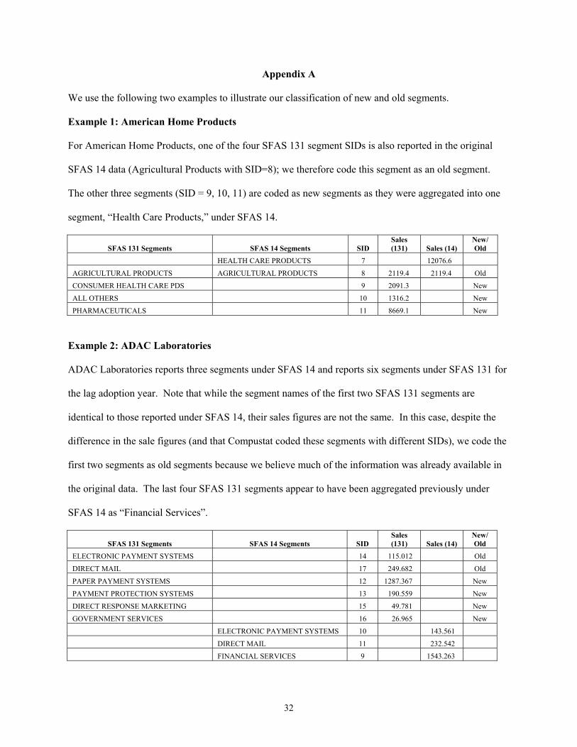
32

Appendix A

We use the following two examples to illustrate our classification of new and old segments.

Example 1: American Home Products For American Home Products, one of the four SFAS 131 segment SIDs is also reported in the original

SFAS 14 data (Agricultural Products with SID=8); we therefore code this segment as an old segment.

The other three segments (SID = 9, 10, 11) are coded as new segments as they were aggregated into one

segment, “Health Care Products,” under SFAS 14.

SFAS 131 Segments SFAS 14 Segments SID Sales (131) Sales (14)

New/ Old

HEALTH CARE PRODUCTS 7 12076.6

AGRICULTURAL PRODUCTS AGRICULTURAL PRODUCTS 8 2119.4 2119.4 Old

CONSUMER HEALTH CARE PDS 9 2091.3 New

ALL OTHERS 10 1316.2 New

PHARMACEUTICALS 11 8669.1 New

Example 2: ADAC Laboratories

ADAC Laboratories reports three segments under SFAS 14 and reports six segments under SFAS 131 for

the lag adoption year. Note that while the segment names of the first two SFAS 131 segments are

identical to those reported under SFAS 14, their sales figures are not the same. In this case, despite the

difference in the sale figures (and that Compustat coded these segments with different SIDs), we code the

first two segments as old segments because we believe much of the information was already available in

the original data. The last four SFAS 131 segments appear to have been aggregated previously under

SFAS 14 as “Financial Services”.

SFAS 131 Segments SFAS 14 Segments SID Sales (131) Sales (14)

New/ Old

ELECTRONIC PAYMENT SYSTEMS 14 115.012 Old

DIRECT MAIL 17 249.682 Old

PAPER PAYMENT SYSTEMS 12 1287.367 New

PAYMENT PROTECTION SYSTEMS 13 190.559 New

DIRECT RESPONSE MARKETING 15 49.781 New

GOVERNMENT SERVICES 16 26.965 New

ELECTRONIC PAYMENT SYSTEMS 10 143.561

DIRECT MAIL 11 232.542

FINANCIAL SERVICES 9 1543.263

33

References

Belsley, D., E. Kuh, R. Welsch. 1980. Regression Diagnostics: Identifying Influential Data and Sources of Collinearity, New York, John Wiley and Sons. Berger, P. and R. Hann. 2003. The Impact of SFAS No. 131 on Information and Monitoring. Journal of Accounting Research 41, 163-223. Berger, P. and E. Ofek. 1995. Diversification's Effect on Firm Value. Journal of Financial Economics 37, 39-65. Botosan, C. and M. Stanford. 2005. Managers’ Motives to Withold Segment Disclosures and the Effect of SFAS No. 131 on Analysts’ Information Enviornment. The Accounting Review 80: 751 – 771. Ernst & Young LLP, 1998. Disclosures about Segments of an Enterprise and Related Information: FASB Statement 131. Ettredge, M., S. Kwon, and D. Smith. 2002. Competitive Harm and Managers’ Attitude Towards SFAS No. 131. Journal of Accounting, Auditing, and Finance 17, 93-109. Financial Accounting Standards Board (FASB). 1976. Financial Reporting for Segments of a Business Enterprise. Statement of Financial Accounting Standards No. 14. Norwalk CT (FASB). Financial Accounting Standards Board (FASB). 1997. Disclosures about Segments of an Enterprise and Related Information. Statement of Financial Accounting Standards No. 131. Norwalk CT (FASB). Givoly, D, C. Hayn, and J. D'Souza. 1999. Measurement Errors and Information Content of Segment Reporting. Review of Accounting Studies 4, 15-43. Harris, M. 1998. The Association between Competition and Managers’ Business Segment Reporting Decisions. Journal of Accounting Research 36, 111-128. Herrmann, D. and W. Thomas. 2000. An Analysis of Segment Disclosures under SFAS No. 131 and SFAS No. 14. Accounting Horizons 14, 287-302. Kennedy, P. A Guide to Econometrics. Cambridge MA: The MIT Press (1992). Lamont, O. 1997. Cash Flow and Investment: Evidence from Internal Capital Markets. Journal of Finance 52, 83-109. Piotroski, J. 2003. Segment Reporting Fineness and the Precision of Investor Beliefs. Working paper, University of Chicago. Puhani, P. 2000. The Heckman Correction for Sample Selection and Its Critique: A Short Survey. Journal of Economic Surveys 14, 53-68. Rajan, R,, H. Servaes and L. Zingales. 2000. The Cost of Diversity: The Diversification Discount and Inefficient Investment. Journal of Finance 55, 35-80. Sanzhar, S. 2003. Two Puzzles about the Diversification Discount: SFAS #131 and ‘Pseudo-Conglomerates.’ Working paper, London Business School.

34

Scott, T. 1994. Incentives and Disincentives for Financial Disclosure: Voluntary Disclosure of Defined Benefit Pension Plan Information by Canadian Firms. Accounting Review 69, 26-43. Shin, H. and R. Stulz. 1998. Are Internal Capital Markets Efficient? Quarterly Journal of Economics 113, 531-552. Street, D., N. Nichols, and S. Gray. 2000. Segment Disclosures under SFAS No. 131: Has Business Segment Reporting Improved? Accounting Horizons 14, 259-285.

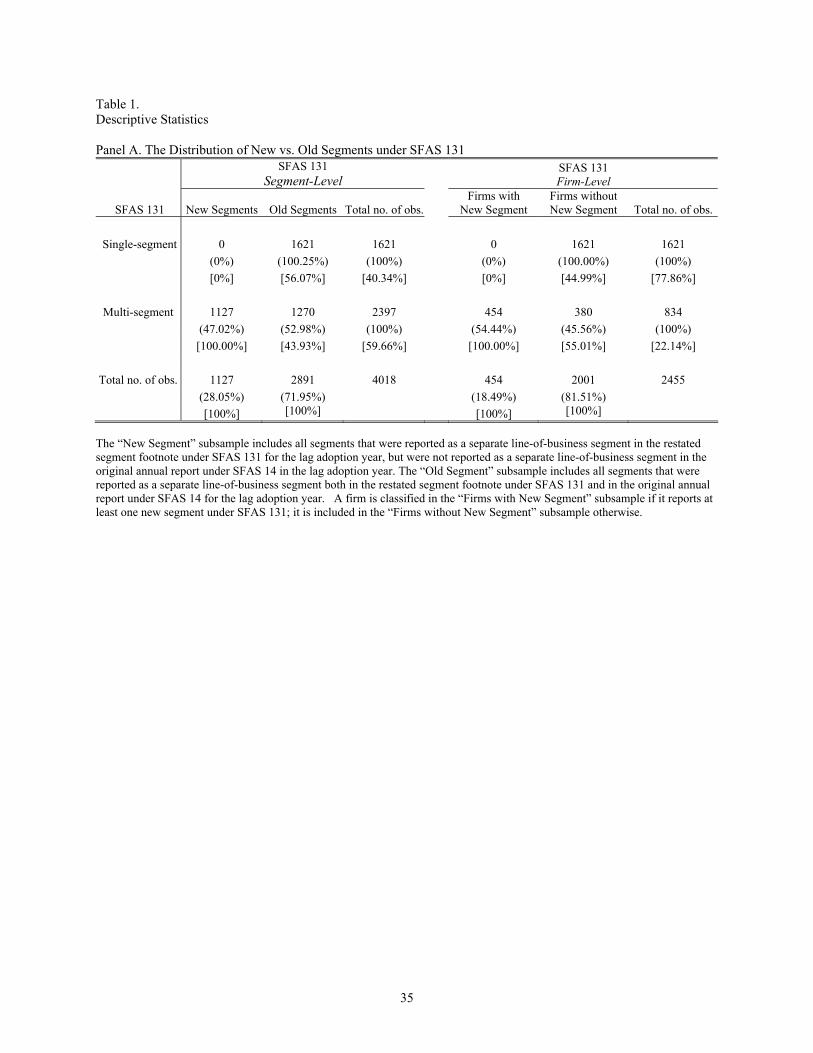
35

Table 1. Descriptive Statistics Panel A. The Distribution of New vs. Old Segments under SFAS 131

SFAS 131

Segment-Level SFAS 131

Firm-Level

SFAS 131 New Segments Old Segments Total no. of obs. Firms with

New Segment Firms without New Segment Total no. of obs.

Single-segment 0 1621 1621 0 1621 1621

(0%) (100.25%) (100%) (0%) (100.00%) (100%) [0%] [56.07%] [40.34%] [0%] [44.99%] [77.86%]

Multi-segment 1127 1270 2397 454 380 834 (47.02%) (52.98%) (100%) (54.44%) (45.56%) (100%) [100.00%] [43.93%] [59.66%] [100.00%] [55.01%] [22.14%]

Total no. of obs. 1127 2891 4018 454 2001 2455 (28.05%) (71.95%) (18.49%) (81.51%) [100%] [100%] [100%] [100%]

The “New Segment” subsample includes all segments that were reported as a separate line-of-business segment in the restated segment footnote under SFAS 131 for the lag adoption year, but were not reported as a separate line-of-business segment in the original annual report under SFAS 14 in the lag adoption year. The “Old Segment” subsample includes all segments that were reported as a separate line-of-business segment both in the restated segment footnote under SFAS 131 and in the original annual report under SFAS 14 for the lag adoption year. A firm is classified in the “Firms with New Segment” subsample if it reports at least one new segment under SFAS 131; it is included in the “Firms without New Segment” subsample otherwise.

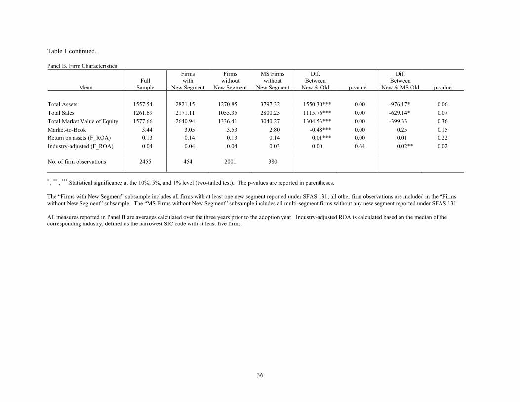
36

Table 1 continued. Panel B. Firm Characteristics

Mean

Full

Sample

Firms with

New Segment

Firms without

New Segment

MS Firms without

New Segment

Dif. Between

New & Old

p-value

Dif. Between

New & MS Old

p-value

Total Assets 1557.54 2821.15 1270.85 3797.32 1550.30*** 0.00 -976.17* 0.06 Total Sales 1261.69 2171.11 1055.35 2800.25 1115.76*** 0.00 -629.14* 0.07 Total Market Value of Equity 1577.66 2640.94 1336.41 3040.27 1304.53*** 0.00 -399.33 0.36 Market-to-Book 3.44 3.05 3.53 2.80 -0.48*** 0.00 0.25 0.15 Return on assets (F_ROA) 0.13 0.14 0.13 0.14 0.01*** 0.00 0.01 0.22 Industry-adjusted (F_ROA) 0.04 0.04 0.04 0.03 0.00 0.64 0.02** 0.02 No. of firm observations

2455

454

2001

380

* , ** , *** Statistical significance at the 10%, 5%, and 1% level (two-tailed test). The p-values are reported in parentheses. The “Firms with New Segment” subsample includes all firms with at least one new segment reported under SFAS 131; all other firm observations are included in the “Firms without New Segment” subsample. The “MS Firms without New Segment” subsample includes all multi-segment firms without any new segment reported under SFAS 131. All measures reported in Panel B are averages calculated over the three years prior to the adoption year. Industry-adjusted ROA is calculated based on the median of the corresponding industry, defined as the narrowest SIC code with at least five firms.

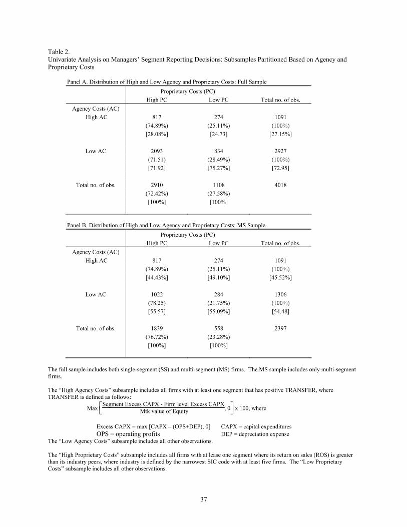
37

Table 2. Univariate Analysis on Managers’ Segment Reporting Decisions: Subsamples Partitioned Based on Agency and Proprietary Costs

Panel A. Distribution of High and Low Agency and Proprietary Costs: Full Sample Proprietary Costs (PC) High PC Low PC Total no. of obs.

Agency Costs (AC) High AC 817 274 1091

(74.89%) (25.11%) (100%) [28.08%] [24.73] [27.15%]

Low AC 2093 834 2927 (71.51) (28.49%) (100%) [71.92] [75.27%] [72.95]

Total no. of obs. 2910 1108 4018 (72.42%) (27.58%) [100%] [100%]

Panel B. Distribution of High and Low Agency and Proprietary Costs: MS Sample

Proprietary Costs (PC) High PC Low PC Total no. of obs.

Agency Costs (AC) High AC 817 274 1091

(74.89%) (25.11%) (100%) [44.43%] [49.10%] [45.52%]

Low AC 1022 284 1306 (78.25) (21.75%) (100%) [55.57] [55.09%] [54.48]

Total no. of obs. 1839 558 2397 (76.72%) (23.28%) [100%] [100%]

The full sample includes both single-segment (SS) and multi-segment (MS) firms. The MS sample includes only multi-segment firms. The “High Agency Costs” subsample includes all firms with at least one segment that has positive TRANSFER, where TRANSFER is defined as follows:

Max Segment Excess CAPX - Firm level Excess CAPX

Mtk value of Equity , 0 x 100, where

Excess CAPX = max [CAPX – (OPS+DEP), 0] CAPX = capital expenditures OPS = operating profits DEP = depreciation expense

The “Low Agency Costs” subsample includes all other observations. The “High Proprietary Costs” subsample includes all firms with at lease one segment where its return on sales (ROS) is greater than its industry peers, where industry is defined by the narrowest SIC code with at least five firms. The “Low Proprietary Costs” subsample includes all other observations.

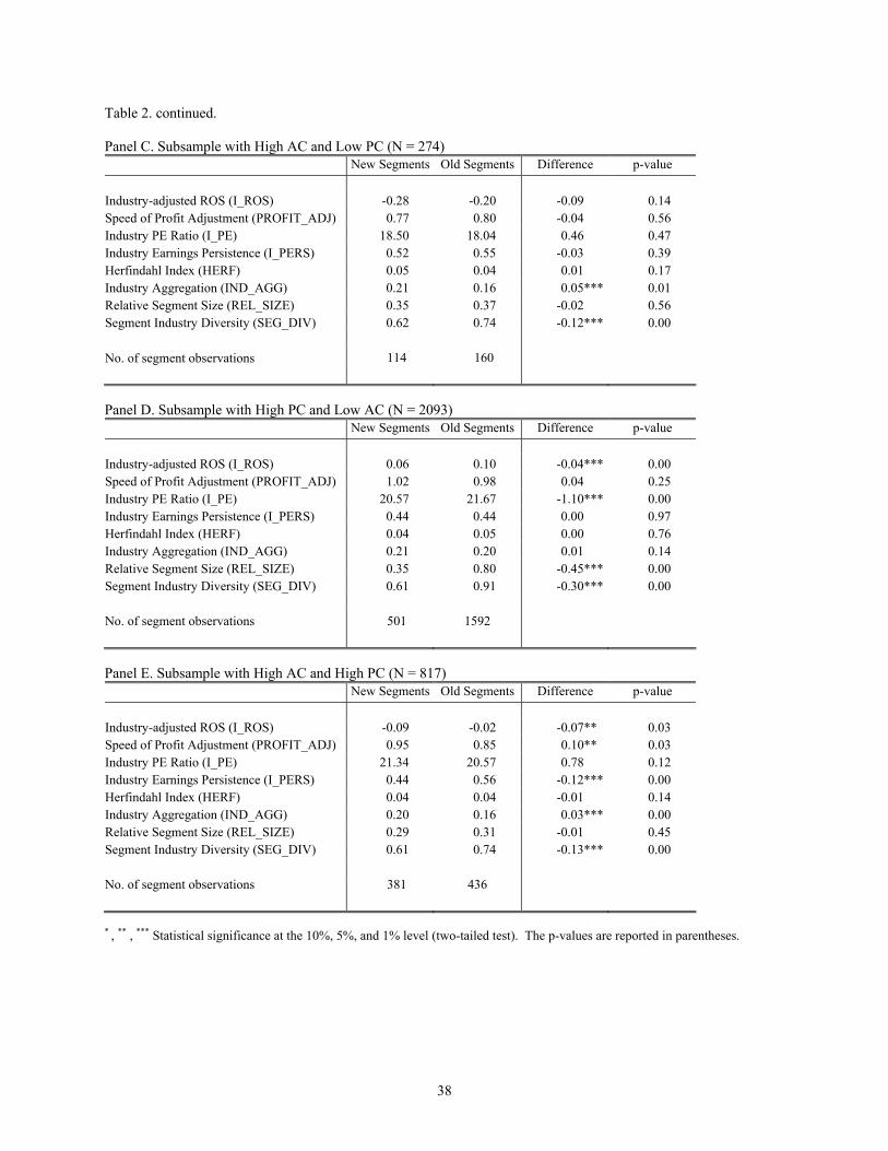
38

Table 2. continued. Panel C. Subsample with High AC and Low PC (N = 274)

New Segments Old Segments Difference p-value Industry-adjusted ROS (I_ROS) -0.28 -0.20 -0.09 0.14 Speed of Profit Adjustment (PROFIT_ADJ) 0.77 0.80 -0.04 0.56 Industry PE Ratio (I_PE) 18.50 18.04 0.46 0.47 Industry Earnings Persistence (I_PERS) 0.52 0.55 -0.03 0.39 Herfindahl Index (HERF) 0.05 0.04 0.01 0.17 Industry Aggregation (IND_AGG) 0.21 0.16 0.05*** 0.01 Relative Segment Size (REL_SIZE) 0.35 0.37 -0.02 0.56 Segment Industry Diversity (SEG_DIV) 0.62 0.74 -0.12*** 0.00 No. of segment observations 114 160 Panel D. Subsample with High PC and Low AC (N = 2093)

New Segments Old Segments Difference p-value Industry-adjusted ROS (I_ROS) 0.06 0.10 -0.04*** 0.00 Speed of Profit Adjustment (PROFIT_ADJ) 1.02 0.98 0.04 0.25 Industry PE Ratio (I_PE) 20.57 21.67 -1.10*** 0.00 Industry Earnings Persistence (I_PERS) 0.44 0.44 0.00 0.97 Herfindahl Index (HERF) 0.04 0.05 0.00 0.76 Industry Aggregation (IND_AGG) 0.21 0.20 0.01 0.14 Relative Segment Size (REL_SIZE) 0.35 0.80 -0.45*** 0.00 Segment Industry Diversity (SEG_DIV) 0.61 0.91 -0.30*** 0.00 No. of segment observations 501 1592

Panel E. Subsample with High AC and High PC (N = 817) New Segments Old Segments Difference p-value

Industry-adjusted ROS (I_ROS) -0.09 -0.02 -0.07** 0.03 Speed of Profit Adjustment (PROFIT_ADJ) 0.95 0.85 0.10** 0.03 Industry PE Ratio (I_PE) 21.34 20.57 0.78 0.12 Industry Earnings Persistence (I_PERS) 0.44 0.56 -0.12*** 0.00 Herfindahl Index (HERF) 0.04 0.04 -0.01 0.14 Industry Aggregation (IND_AGG) 0.20 0.16 0.03*** 0.00 Relative Segment Size (REL_SIZE) 0.29 0.31 -0.01 0.45 Segment Industry Diversity (SEG_DIV) 0.61 0.74 -0.13*** 0.00 No. of segment observations 381 436 * , ** , *** Statistical significance at the 10%, 5%, and 1% level (two-tailed test). The p-values are reported in parentheses.

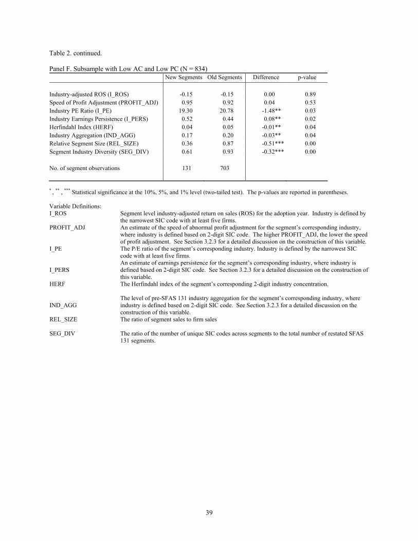
39

Table 2. continued. Panel F. Subsample with Low AC and Low PC (N = 834)

New Segments Old Segments Difference p-value Industry-adjusted ROS (I_ROS) -0.15 -0.15 0.00 0.89 Speed of Profit Adjustment (PROFIT_ADJ) 0.95 0.92 0.04 0.53 Industry PE Ratio (I_PE) 19.30 20.78 -1.48** 0.03 Industry Earnings Persistence (I_PERS) 0.52 0.44 0.08** 0.02 Herfindahl Index (HERF) 0.04 0.05 -0.01** 0.04 Industry Aggregation (IND_AGG) 0.17 0.20 -0.03** 0.04 Relative Segment Size (REL_SIZE) 0.36 0.87 -0.51*** 0.00 Segment Industry Diversity (SEG_DIV) 0.61 0.93 -0.32*** 0.00 No. of segment observations 131 703

* , ** , *** Statistical significance at the 10%, 5%, and 1% level (two-tailed test). The p-values are reported in parentheses. Variable Definitions: I_ROS

Segment level industry-adjusted return on sales (ROS) for the adoption year. Industry is defined by the narrowest SIC code with at least five firms.

PROFIT_ADJ

An estimate of the speed of abnormal profit adjustment for the segment’s corresponding industry, where industry is defined based on 2-digit SIC code. The higher PROFIT_ADJ, the lower the speed of profit adjustment. See Section 3.2.3 for a detailed discussion on the construction of this variable.

I_PE

The P/E ratio of the segment’s corresponding industry. Industry is defined by the narrowest SIC code with at least five firms.

I_PERS

An estimate of earnings persistence for the segment’s corresponding industry, where industry is defined based on 2-digit SIC code. See Section 3.2.3 for a detailed discussion on the construction of this variable.

HERF

The Herfindahl index of the segment’s corresponding 2-digit industry concentration.

IND_AGG

The level of pre-SFAS 131 industry aggregation for the segment’s corresponding industry, where industry is defined based on 2-digit SIC code. See Section 3.2.3 for a detailed discussion on the construction of this variable.

REL_SIZE

The ratio of segment sales to firm sales

SEG_DIV

The ratio of the number of unique SIC codes across segments to the total number of restated SFAS 131 segments.

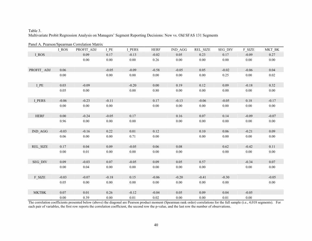
40

Table 3. Multivariate Probit Regression Analysis on Managers’ Segment Reporting Decisions: New vs. Old SFAS 131 Segments Panel A. Pearson/Spearman Correlation Matrix

I_ROS PROFIT_ADJ I_PE I_PERS HERF IND_AGG REL_SIZE SEG_DIV F_SIZE MKT_BK I_ROS 0.09 0.17 -0.13 -0.02 0.05 0.23 0.17 -0.09 0.27

0.00 0.00 0.00 0.26 0.00 0.00 0.00 0.00 0.00

PROFIT_ ADJ 0.06 -0.05 -0.09 -0.58 -0.05 0.05 -0.02 -0.06 0.04 0.00 0.00 0.00 0.00 0.00 0.00 0.25 0.00 0.02

I_PE 0.03 -0.09 -0.20 0.00 0.19 0.12 0.09 -0.18 0.32 0.05 0.00 0.00 0.80 0.00 0.00 0.00 0.00 0.00

I_PERS -0.06 -0.23 -0.11 0.17 -0.13 -0.06 -0.05 0.18 -0.17 0.00 0.00 0.00 0.00 0.00 0.00 0.00 0.00 0.00

HERF 0.00 -0.24 -0.05 0.17 0.16 0.07 0.14 -0.09 -0.07 0.96 0.00 0.00 0.00 0.00 0.00 0.00 0.00 0.00

IND_AGG -0.03 -0.16 0.22 0.01 0.12 0.10 0.06 -0.21 0.09 0.06 0.00 0.00 0.71 0.00 0.00 0.00 0.00 0.00

REL_SIZE 0.17 0.04 0.09 -0.05 0.06 0.08 0.62 -0.42 0.11 0.00 0.01 0.00 0.00 0.00 0.00 0.00 0.00 0.00

SEG_DIV 0.09 -0.03 0.07 -0.05 0.09 0.05 0.57 -0.34 0.07 0.00 0.04 0.00 0.00 0.00 0.00 0.00 0.00 0.00

F_SIZE -0.03 -0.07 -0.18 0.15 -0.06 -0.20 -0.41 -0.30 -0.05 0.05 0.00 0.00 0.00 0.00 0.00 0.00 0.00 0.00

MKTBK 0.07 0.01 0.26 -0.12 -0.04 0.05 0.09 0.04 -0.05 0.00 0.39 0.00 0.01 0.02 0.00 0.00 0.01 0.00

The correlation coefficients presented below (above) the diagonal are Pearson product moment (Spearman rank order) correlations for the full sample (i.e., 4,018 segments). For each pair of variables, the first row reports the correlation coefficient, the second row the p-value, and the last row the number of observations.

41

Table 3 continued.

Variable Definitions:

I_ROS

Segment level industry-adjusted return on sales (ROS) for the adoption year. Industry is defined by the narrowest SIC code with at least five firms.

PROFIT_ADJ

An estimate of the speed of abnormal profit adjustment for the segment’s corresponding industry, where industry is defined based on 2-digit SIC code. The higher PROFIT_ADJ, the lower the speed of profit adjustment. See Section 3.2.3 for a detailed discussion on the construction of this variable.

I_PE

The P/E ratio of the segment’s corresponding industry. Industry is defined by the narrowest SIC code with at least five firms.

I_PERS

An estimate of earnings persistence for the segment’s corresponding industry, where industry is defined based on 2-digit SIC code. See Section 3.2.3 for a detailed discussion on the construction of this variable.

HERF

The Herfindahl index of the segment’s corresponding 2-digit industry concentration.

IND_AGG

The level of pre-SFAS 131 industry aggregation for the segment’s corresponding industry, where industry is defined based on 2-digit SIC code. See Section 3.2.3 for a detailed discussion on the construction of this variable.

REL_SIZE

The ratio of segment sales to firm sales

SEG_DIVERSITY

The ratio of the number of unique SIC codes across segments to the total number of restated SFAS 131 segments.

F_SIZE

The average of the log of the firm’s total assets over the three years prior to the adoption year.

MKTBK

The average ratio of the firm’s market value of equity to book value of equity over the three year prior to the adoption year.

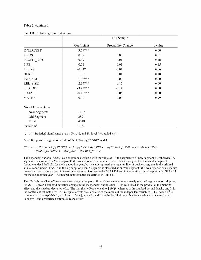
42

Table 3. continued Panel B. Probit Regression Analysis

Full Sample

Coefficient

Probability Change p-value INTERCEPT 3.79*** 0.00 I_ROS 0.08 0.00 0.51 PROFIT_ADJ 0.09 0.01 0.18 I_PE -0.01 -0.01 0.15 I_PERS -0.24* -0.01 0.06 HERF 1.30 0.01 0.10 IND_AGG 1.06*** 0.03 0.00 REL_SIZE -2.35*** -0.15 0.00 SEG_DIV -3.42*** -0.14 0.00 F_SIZE -0.16*** -0.05 0.00 MKTBK 0.00 0.00 0.99

No. of Observations:

New Segments 1127 Old Segments 2891 Total 4018 Pseudo R2 0.27

* , ** , *** Statistical significance at the 10%, 5%, and 1% level (two-tailed test). Panel B reports the regression results of the following PROBIT model: NEW = α + β1 I_ROS + β2 PROFIT_ADJ + β3 I_PE + β4 I_PERS + β5 HERF + β6 IND_AGG + β7 REL_SIZE

+ β8 SEG_DIVERSITY + β9 F_SIZE + β10 MKT_BK + ε, The dependent variable, NEW, is a dichotomous variable with the value of 1 if the segment is a “new segment”; 0 otherwise. A segment is classified as a “new segment” if it was reported as a separate line-of-business segment in the restated segment footnote under SFAS 131 for the lag adoption year, but was not reported as a separate line-of-business segment in the original annual report under SFAS 14 in the lag adoption year. A segment is classified as an “old segment” if it was reported as a separate line-of-business segment both in the restated segment footnote under SFAS 131 and in the original annual report under SFAS 14 for the lag adoption year. The independent variables are defined in Table 2. The “Probability Change” measures the change in the probability of the segment being a newly reported segment upon adopting SFAS 131, given a standard deviation change in the independent variables (xi). It is calculated as the product of the marginal effect and the standard deviation of xi. The marginal effect is equal to ф(βx)βi, where ф is the standard normal density and βi is the coefficient estimate of xi. All marginal effects are calculated at the means of the independent variables. The Pseudo R2 is computed as: 1 – exp[-2(ln Lr – ln L)/no. of obs.], where Lr and L are the log-likelihood functions evaluated at the restricted (slopes=0) and unrestricted estimates, respectively.

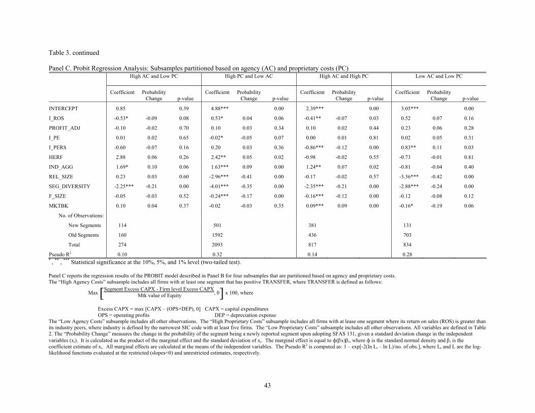
43

Table 3. continued Panel C. Probit Regression Analysis: Subsamples partitioned based on agency (AC) and proprietary costs (PC)

High AC and Low PC

High PC and Low AC

High AC and High PC

Low AC and Low PC

Coefficient Probability

Change p-value Coefficient Probability

Change p-value Coefficient Probability

Change p-value Coefficient Probability

Change p-value

INTERCEPT 0.85 0.39 4.88*** 0.00 2.39*** 0.00 3.05*** 0.00

I_ROS -0.53* -0.09 0.08 0.53* 0.04 0.06 -0.41** -0.07 0.03 0.52 0.07 0.16

PROFIT_ADJ -0.10 -0.02 0.70 0.10 0.03 0.34 0.10 0.02 0.44 0.23 0.06 0.28

I_PE 0.01 0.02 0.65 -0.02* -0.05 0.07 0.00 0.01 0.81 0.02 0.05 0.31

I_PERS -0.60 -0.07 0.16 0.20 0.03 0.36 -0.86*** -0.12 0.00 0.83** 0.11 0.03

HERF 2.88 0.06 0.26 2.42** 0.05 0.02 -0.98 -0.02 0.55 -0.73 -0.01 0.81

IND_AGG 1.69* 0.10 0.06 1.63*** 0.09 0.00 1.24** 0.07 0.02 -0.81 -0.04 0.40

REL_SIZE 0.23 0.03 0.60 -2.96*** -0.41 0.00 -0.17 -0.02 0.57 -3.36*** -0.42 0.00

SEG_DIVERSITY -2.25*** -0.21 0.00 -4.01*** -0.35 0.00 -2.35*** -0.21 0.00 -2.88*** -0.24 0.00

F_SIZE -0.05 -0.03 0.52 -0.24*** -0.17 0.00 -0.16*** -0.12 0.00 -0.12 -0.08 0.12

MKTBK 0.10 0.04 0.37 -0.02 -0.03 0.35 0.09*** 0.09 0.00 -0.16* -0.19 0.06

No. of Observations:

New Segments 114 501 381 131

Old Segments 160 1592 436 703

Total 274 2093 817 834

Pseudo R2 0.10 0.32 0.14 0.28 * , ** , *** Statistical significance at the 10%, 5%, and 1% level (two-tailed test). Panel C reports the regression results of the PROBIT model described in Panel B for four subsamples that are partitioned based on agency and proprietary costs. The “High Agency Costs” subsample includes all firms with at least one segment that has positive TRANSFER, where TRANSFER is defined as follows:

Max [ ]Segment Excess CAPX - Firm level Excess CAPX

Mtk value of Equity , 0 x 100, where

Excess CAPX = max [CAPX – (OPS+DEP), 0] CAPX = capital expenditures OPS = operating profits DEP = depreciation expense

The “Low Agency Costs” subsample includes all other observations. The “High Proprietary Costs” subsample includes all firms with at lease one segment where its return on sales (ROS) is greater than its industry peers, where industry is defined by the narrowest SIC code with at least five firms. The “Low Proprietary Costs” subsample includes all other observations. All variables are defined in Table 2. The “Probability Change” measures the change in the probability of the segment being a newly reported segment upon adopting SFAS 131, given a standard deviation change in the independent variables (xi). It is calculated as the product of the marginal effect and the standard deviation of xi. The marginal effect is equal to ф(βx)βi, where ф is the standard normal density and βi is the coefficient estimate of xi. All marginal effects are calculated at the means of the independent variables. The Pseudo R2 is computed as: 1 – exp[-2(ln Lr – ln L)/no. of obs.], where Lr and L are the log-likelihood functions evaluated at the restricted (slopes=0) and unrestricted estimates, respectively.

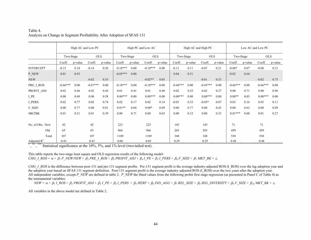
44

Table 4. Analysis on Change in Segment Profitability After Adoption of SFAS 131

High AC and Low PC

High PC and Low AC

High AC and High PC

Low AC and Low PC

Two-Stage OLS Two-Stage OLS Two-Stage OLS Two-Stage OLS

Coeff. p-value Coeff. p-value Coeff. p-value Coeff. p-value Coeff. p-value Coeff. p-value Coeff. p-value Coeff. p-value

INTERCEPT -0.15 0.18 -0.14 0.20 -0.10*** 0.00 -0.10*** 0.00 -0.11 0.11 -0.07 0.21 -0.08* 0.07 -0.08 0.31

P_NEW 0.01 0.93 -0.05*** 0.00 0.04 0.51 -0.02 0.64

NEW -0.02 0.55 -0.02** 0.05 -0.01 0.53 -0.02 0.75

PRE_I_ROS -0.66*** 0.00 -0.67*** 0.00 -0.10*** 0.00 -0.10*** 0.00 -0.44*** 0.00 -0.45*** 0.00 -0.66*** 0.00 -0.66*** 0.00

PROFIT_ADJ 0.02 0.46 0.02 0.44 0.01 0.41 0.01 0.40 0.02 0.25 0.02 0.27 0.00 0.71 0.00 0.96

I_PE 0.00 0.69 0.00 0.58 0.00*** 0.00 0.00*** 0.00 0.00*** 0.00 0.00*** 0.00 0.00** 0.03 0.00*** 0.00

I_PERS 0.02 0.77 0.02 0.74 0.02 0.17 0.02 0.14 -0.03 0.33 -0.05* 0.07 0.03 0.16 0.03 0.11

F_SIZE 0.00 0.77 0.00 0.91 0.01** 0.04 0.00* 0.09 0.00 0.77 0.00 0.43 0.00 0.62 0.00 0.89

MKTBK 0.01 0.51 0.01 0.39 0.00 0.71 0.00 0.65 0.00 0.33 0.00 0.33 0.01*** 0.00 0.01 0.27

No. of Obs: New 42 42 223 223 145 145 71 71

Old 65 65 966 966 203 203 459 459

Total 107 107 1189 1189 348 348 530 530 Adjusted R2 0.43 0.43 0.06 0.05 0.29 0.29 0.48 0.48 * , ** , *** Statistical significance at the 10%, 5%, and 1% level (two-tailed test). This table reports the two-stage least square and OLS regression results of the following model: CHG_I_ROS = α + β1 P_NEW/NEW + β2 PRE_I_ROS + β3 PROFIT_ADJ + β4 I_PE + β5 I_PERS + β6 F_SIZE + β7 MKT_BK + ε, CHG_I_ROS is the difference between post-131 and pre-131 segment profits. Pre-131 segment profit is the average industry-adjusted ROS (I_ROS) over the lag adoption year and the adoption year based on SFAS 131 segment definition. Post-131 segment profit is the average industry-adjusted ROS (I_ROS) over the two years after the adoption year. All independent variables, except P_NEW are defined in table 2. P_NEW the fitted values from the following probit first stage regression (as presented in Panel C of Table 4) as the instrumental variables: NEW = α + β1 I_ROS + β2 PROFIT_ADJ + β3 I_PE + β4 I_PERS + β5 HERF + β6 IND_AGG + β7 REL_SIZE + β8 SEG_DIVERSITY + β9 F_SIZE + β10 MKT_BK + ε, All variables in the above model are defined in Table 2.