Embed Size (px)
Citation preview

ARTICLE IN PRESS
0098-3004/$ - se
doi:10.1016/j.ca
$Code availa
index.htm.�Correspond
fax: +1418 724
E-mail addr
c.ferrarin@ism
(C.L. Amos),
Universite du
Rimouski, QC,
Computers & Geosciences 34 (2008) 1223–1242
www.elsevier.com/locate/cageo
Sedtrans05: An improved sediment-transport model forcontinental shelves and coastal waters with a new
algorithm for cohesive sediments$
Urs Neumeiera,�,1, Christian Ferrarinb, Carl L. Amosa,Georg Umgiesserb, Michael Z. Lic
aSchool of Ocean and Earth Science, National Oceanography Centre, University of Southampton, European Way,
Southampton SO14 3ZH, UKbISMAR-CNR Venice, Venezia, Italy
cGeological Survey of Canada, Bedford Institute of Oceanography, P.O. Box 1006, Dartmouth, Nova Scotia, Canada B2Y 4A2
Received 16 October 2006
Abstract
The one-dimensional (vertical) sediment-transport model SEDTRANS96 has been upgraded to predict more accurately
both cohesive and non-cohesive sediment transport. Sedtrans05 computes the bed shear stress for a given set of flow and
seabed conditions using combined wave-current bottom boundary layer theory. Sediment transport (bedload and total
load) is evaluated using one of five methods. The main modifications to the original version of the model are: (1) a
reorganization of the code so that the computation routines can be easily accessed from different user interfaces, or may be
called from other programs; (2) the addition of the Van Rijn method to the options for non-cohesive sediment transport;
(3) the computation of density and viscosity of water from temperature and salinity inputs; and (4) the addition of a new
cohesive sediment algorithm. This latter algorithm introduces variations of sediment properties with depth, represents the
suspended sediment as a spectrum of settling velocities (i.e. size classes), includes the flocculation process, and models
multiple erosion–deposition cycles. The new model matches slightly better the field measurements of non-cohesive
sediment transport, than does the predictions by SEDTRANS96. The sand-transport calibration has been extended to high
transport rates. The cohesive sediment algorithm reproduced well experimental data from annular flume experiments.
r 2008 Elsevier Ltd. All rights reserved.
Keywords: Cohesive sediment transport; Sand transport; Numerical model; Sediment dynamics; Continental shelf; Estuarine processes
e front matter r 2008 Elsevier Ltd. All rights reserved
geo.2008.02.007
ble from server at http://www.iamg.org/CGEditor/
ing author. Tel.: +1418 7231986x1278;
1842.
esses: [email protected] (U. Neumeier),
ar.cnr.it (C. Ferrarin), [email protected]
[email protected] (G. Umgiesser),
a (M.Z. Li).
ress: Institut des sciences de la mer de Rimouski,
Quebec a Rimouski, 310 allee des Ursulines,
Canada G5L 1G3.
1. Introduction
Predicting the transport of non-cohesive (sand)and cohesive (mud) sediments in estuaries and oncontinental shelves is of great practical importanceas these processes can have significant impacts onseabed stability, on the dispersal of particulatematerial, and on benthic habitat distribution.
.

ARTICLE IN PRESS
Nomenclature
Aulva bed fraction covered by vegetationC0 initial SSC (kgm�3)Cdr constant for the drag reduction formula
(m3 kg�1)Csolid coefficient for the solid-transmitted stress
by free-moving vegetationCt SSC after time t (kgm�3)C(i) SSC of each Ws class (kgm
�3)D (median) sediment grain diameter
(m)Dt constant for turbulent disruption during
erosionD* dimensionless grain sizeE0 empirical coefficient for minimum ero-
sion (kgm�2 s�1)Fk flocculation coefficientFm flocculation coefficientg gravity (m s�1)h water depth (m)Hs significant wave height (m)kcd coefficient for the relationship between
tcd and Ws
mcd coefficient for the relationship betweentcd and Ws
mo dry mass of overlaying sediment (kgm�2)Pe proportionality coefficient for erosion
(Pa�0.5)Ps probability coefficient of resuspensionq bedload transport rate (m2 s�1)rd deposition rate of cohesive sediment
(kgm�2 s�1)re erosion rate of cohesive sediment
(kgm�2 s�1)S salinity (practical salinity scale)
SSC suspended sediment concentration(kgm�3)
t, Dt time, time interval (s)u*crs critical shear velocity for sediment sus-
pension (m s�1)T temperature (1C)Tm dimensionless shear stress parameterWs settling velocity (m s�1)WsFloc settling velocity corrected for flocculation
and hindered settling (m s�1)z depth below sediment surface for cohe-
sive bed (m)z0 bed roughness (m)Z dynamic viscosity (Pa s)n kinematic viscosity (m2 s�1)r fluid density (kgm�3)rclay density of the clay minerals (kgm�3)rdry dry bulk density of cohesive bed (kgm�3)rs density of non-cohesive sediment
(kgm�3)rwet wet bulk density of sediment (kgm�3)t0 bed shear stress (Pa)tcd critical deposition shear stress for cohe-
sive sediment (Pa)tce critical erosion shear stress for cohesive
sediment (Pa)tcrb critical shear stress for initiation of bed-
load motion (Pa)tcs instantaneous skin-friction current shear
stress (Pa)tcws the instantaneous skin-friction combined
shear stress (Pa)tmUlva threshold of motion of vegetation (Pa)tresUlva threshold of full resuspension of vegeta-
tion (Pa)tsolid solid-transmitted stress (Pa)
U. Neumeier et al. / Computers & Geosciences 34 (2008) 1223–12421224
Sediment-transport modelling started with thedevelopment of analytical and 1-D models (DeVries et al., 1989; Dyer and Evans, 1989; Grant andMadsen, 1979; Ross and Mehta, 1989; Smith, 1977;Wiberg et al., 1994). Due to recent advances inhydrodynamic and wave modelling as well as theincrease in computing power, depth-averaged two-dimensional models (Harris and Wiberg, 2001; Liet al., 1994; Mulder and Udink, 1991) and three-dimensional models (Le Normant, 2000; Lesseret al., 2004; Pandoe and Edge, 2004) have evolved.The sophistication of model structure appears tohave outstripped the understanding of sedimentary
processes such as flocculation, consolidation, sand–mud interactions, and the theories on which they arebased.
This paper describes the implementation ofSedtrans05, a one-dimensional (vertical) numericalmodel, which accounts more accurately thanhitherto the complex sedimentary processes ofcoastal environments, giving not only boundarylayer parameters but also predicting bedformdevelopment, bedload as well as suspended loadtransport rates for both sand and cohesive sedi-ments. Our ability to realistically simulate sedimenttransport is often limited by our ability to formulate

ARTICLE IN PRESSU. Neumeier et al. / Computers & Geosciences 34 (2008) 1223–1242 1225
essential sediment processes, not by the efficiencyand sophistication of our numerical models. Sed-trans05 has been developed as a 1D model to testthe model behaviour, to compare various algo-rithms between each other, and to calibrate themwith field data. The simplicity and flexibility of 1Dmodels also facilitate the incorporation of newprocesses, especially for cohesive sediments. On theother hand, multi-dimension models are needed toaddress spatial variability and seabed deposition/erosion pattern. However, once a 1D model hasbeen tested it can be easily integrated into other 2D/3D models; see Ferrarin et al. (2004) for an exampleof integration of Sedtrans05 in a 3D hydrodynamicmodel.
Sedtrans05 is the latest version of SEDTRANS,which was developed more than 20 years ago(Davidson and Amos, 1985; Martec Ltd., 1987;unpublished reports by Martec Ltd.2). The twolatest versions were SEDTRANS92 (Li and Amos,1995) and SEDTRANS96 (Li and Amos, 2001).Sedtrans05 differs from SEDTRANS96 in severalfundamental ways. The Fortran77 code is restruc-tured so that all computations of the hydrody-namics and resulting sediment transport areaccessed through a single subroutine that can becalled from various programs. A new cohesivesediment algorithm is developed: (1) it providesdetailed variations of sediment properties withdepth, (2) it represents the suspended sediment asa spectrum of settling velocities (i.e. size classes), (3)it includes the flocculation process, and (4) itprovides simulations of multiple erosion–depositioncycles. The Van Rijn (1993) method has been addedto the equations available for prediction of non-cohesive sediment transport. Still water settlingvelocity of sand is computed with the equation ofSoulsby (1997). Also, the density and viscosity ofwater are computed from temperature and salinityinput data.
2. Model structure and program operation
Sedtrans05 is a one-dimensional (vertical profiles)model of sediment transport that simulates either
2Martec Ltd., 1984. SED1D: a sediment transport model for
the continental shelf. Unpublished report submitted to Geologi-
cal Survey of Canada, DSS Contract no. 10SC 23420-3-M753,
63pp. Martec Ltd., 1990. Upgrading and application of the AGC
sediment transport model SEDTRANS. Unpublished report
submitted to Geological Survey of Canada, SCC Contract no.
23420-0-M166/01-OSC, 56pp.
sand or cohesive sediments under either steadycurrents or under the combined influences of wavesand currents. Sedtrans05 uses the Grant andMadsen (1986) continental shelf bottom boundarylayer theory to predict the mean bed shear stressesand the combined velocity profile.
Five methods to predict sediment transport fornon-cohesive sediments are programmed into thenewer version. The methods of Einstein–Brown(Brown, 1950), Yalin (1963), and Van Rijn (1993)predict bedload transport. The methods of Enge-lund and Hansen (1967) and Bagnold (1963) predicttotal load transport (bedload plus suspended load).The dimensions and type of bedforms are alsopredicted. A new algorithm for cohesive sedimentsdetermines more accurately bed erosion and deposi-tion (see Section 4).
Sedtrans05 is composed of several linked ele-ments. The calculations are coded in a set ofFortran77 routines that are accessed through thesubroutine SEDTRANS05. This subroutine takesas input current and wave conditions and sedimenttype (Table 1). After calling the appropriatesubroutines, the model returns the results as output.
The core subroutine SEDTRANS05 can be calledin several ways: (1) as an interactive input and batchprogram—SED05—which runs in a console win-dow; (2) as a graphic user interface—Sedtrans05GUI—written in Visual Basic and running underMicrosoft Windows; (3) as a MEX-file function tocall the Fortran77 subroutines directly from Ma-tlab—sedtrans05m; (4) as a 1D (time series) modelfor cohesive sediment—SEDI1D—which was usedto calibrate the cohesive sediment algorithm (seeSection 5.2); and (5) as a subroutine linked to a 3Dhydrodynamic model, such as the model SHYFEM,which simulates waves and tidal flows in Venicelagoon (Ferrarin et al., 2004; Umgiesser et al.,2006).
Sedtrans05 can be used as 1D model or integratedinto a multi-dimensional model. The difference issimply that in the 1D interface the velocities andwave parameters are prescribed as external forcing,supplied by the user, whereas in a 2D/3D modelthese values are supplied directly by the hydro-dynamic model. Likewise, the output of Sedtrans05is simply written to output files for a 1D interface,whereas, when integrated in a multi-dimensionalmodel, the output is fed back to the hydrodynamicmodel to change the bathymetry; it thereforeprovides feedback from the sediment dynamics tothe hydrodynamics.
ARTICLE IN PRESS
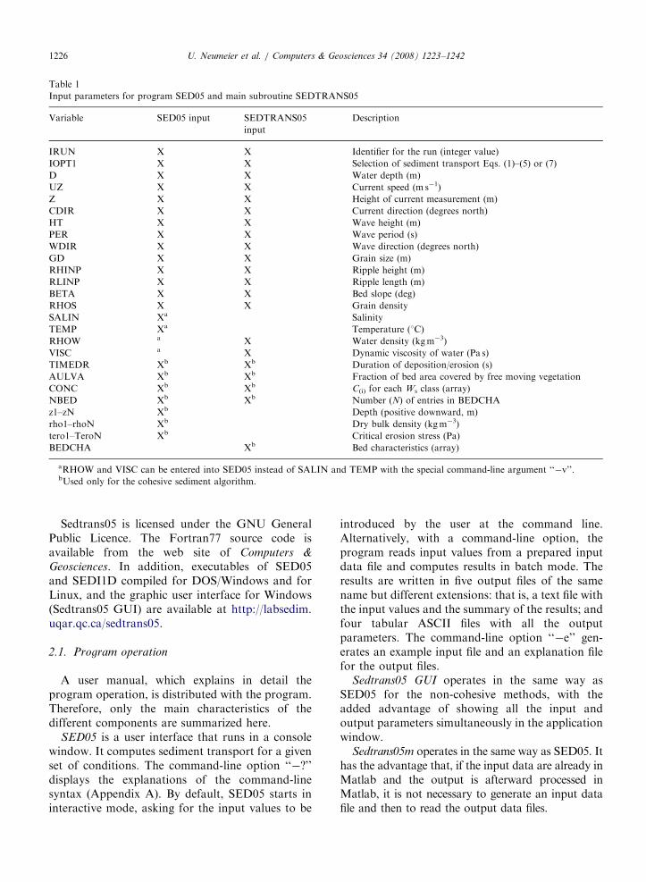
Table 1
Input parameters for program SED05 and main subroutine SEDTRANS05
Variable SED05 input SEDTRANS05
input
Description
IRUN X X Identifier for the run (integer value)
IOPT1 X X Selection of sediment transport Eqs. (1)–(5) or (7)
D X X Water depth (m)
UZ X X Current speed (m s�1)
Z X X Height of current measurement (m)
CDIR X X Current direction (degrees north)
HT X X Wave height (m)
PER X X Wave period (s)
WDIR X X Wave direction (degrees north)
GD X X Grain size (m)
RHINP X X Ripple height (m)
RLINP X X Ripple length (m)
BETA X X Bed slope (deg)
RHOS X X Grain density
SALIN Xa Salinity
TEMP Xa Temperature (1C)
RHOW a X Water density (kgm�3)
VISC a X Dynamic viscosity of water (Pa s)
TIMEDR Xb Xb Duration of deposition/erosion (s)
AULVA Xb Xb Fraction of bed area covered by free moving vegetation
CONC Xb Xb C(i) for each Ws class (array)
NBED Xb Xb Number (N) of entries in BEDCHA
z1–zN Xb Depth (positive downward, m)
rho1–rhoN Xb Dry bulk density (kgm�3)
tero1–TeroN Xb Critical erosion stress (Pa)
BEDCHA Xb Bed characteristics (array)
aRHOW and VISC can be entered into SED05 instead of SALIN and TEMP with the special command-line argument ‘‘�v’’.bUsed only for the cohesive sediment algorithm.
U. Neumeier et al. / Computers & Geosciences 34 (2008) 1223–12421226
Sedtrans05 is licensed under the GNU GeneralPublic Licence. The Fortran77 source code isavailable from the web site of Computers &
Geosciences. In addition, executables of SED05and SEDI1D compiled for DOS/Windows and forLinux, and the graphic user interface for Windows(Sedtrans05 GUI) are available at http://labsedim.uqar.qc.ca/sedtrans05.
2.1. Program operation
A user manual, which explains in detail theprogram operation, is distributed with the program.Therefore, only the main characteristics of thedifferent components are summarized here.
SED05 is a user interface that runs in a consolewindow. It computes sediment transport for a givenset of conditions. The command-line option ‘‘�?’’displays the explanations of the command-linesyntax (Appendix A). By default, SED05 starts ininteractive mode, asking for the input values to be
introduced by the user at the command line.Alternatively, with a command-line option, theprogram reads input values from a prepared inputdata file and computes results in batch mode. Theresults are written in five output files of the samename but different extensions: that is, a text file withthe input values and the summary of the results; andfour tabular ASCII files with all the outputparameters. The command-line option ‘‘�e’’ gen-erates an example input file and an explanation filefor the output files.
Sedtrans05 GUI operates in the same way asSED05 for the non-cohesive methods, with theadded advantage of showing all the input andoutput parameters simultaneously in the applicationwindow.
Sedtrans05m operates in the same way as SED05. Ithas the advantage that, if the input data are already inMatlab and the output is afterward processed inMatlab, it is not necessary to generate an input datafile and then to read the output data files.
ARTICLE IN PRESS
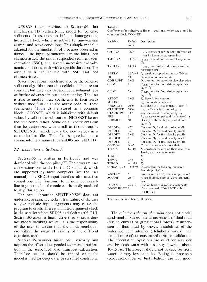
Table 2
Coefficients for cohesive sediment equations, which are stored in
common block CCONST
Variable Default
value
Description
CSULVA 159.4 Csolid coefficient for the solid-transmitted
stress by free-moving vegetation
TMULVA 1.054e�3 tmUlva threshold of motion of vegetation
(Pa)
TRULVA 0.0013 tresUlva threshold of full resuspension of
vegetation (Pa)
RKERO 1.95e�5 Pe, erosion proportionality coefficient
E0 5.88 E0, minimum erosion rate
CDISRUPT 0.001 Dt, constant for turbulent floc disruption
CLIM1 0.1 CLIM1, limit for flocculation equations
(kgm�3)
CLIM2 2.0 CLIM2, limit for flocculation equations
(kgm�3)
KFLOC 0.001 Fk, flocculation constant
MFLOC 1 Fm, flocculation constant
RHOCLAY 2600 rclay, density of clay minerals (kgm�3)
CTAUDEPK 2800 kcd, coefficient for computing tcdCTAUDEPM 1.03 mcd, coefficient for computing tcdPRS 0 Ps, resuspension probability (range 0–1)
RHOMUD 50 Density of the freshly deposited mud
(kgm�3)
DPROFA 470 Constant Da for final density profile
DPROFB 150 Constant Db for final density profile
DPROFC 0.015 Constant Dc for final density profile
DPROFD 0 Constant Dd for final density profile
DPROFE 0 Constant De for final density profile
CONSOA 1e�5 Ca time constant of consolidation
TEROA 6e�10 Ta constants for erosion threshold from
density and overlaying mass
TEROB 3 Tb
TEROC 3.47 Tc
TEROD �1.915 Td
CDRAGRED �0.0893 Cdr constant for the drag reduction
formula (m3 kg�1)
WSCLAY 5 Primary median Ws class (integer value)
ZOCOH 2e�4 z0 bed roughness for cohesive sediments
(m)
FCWCOH 2.2e�3 Friction factor for cohesive sediments
DOCOMPACT 0 If not zero, call COMPACT within
COHESIVE
They can be modified by the user.
U. Neumeier et al. / Computers & Geosciences 34 (2008) 1223–1242 1227
SEDI1D is an interface to Sedtrans05 thatsimulates a 1D (vertical)-time model for cohesivesediments. It assumes an infinite, homogeneous,horizontal bed, which is subject to time-varyingcurrent and wave conditions. This simple model isadapted for the simulation of processes observed influmes. The input parameters are the initial bedcharacteristics, the initial suspended sediment con-centration (SSC), and several successive hydrody-namic conditions, each with a specific duration. Theoutput is a tabular file with SSC and bedcharacteristics.
Several equations, which are used by the cohesivesediment algorithm, contain coefficients that are notconstant, but may vary depending on sediment typeor further advances in our understanding. The useris able to modify these coefficients to their needswithout modification to the source code. All thesecoefficients (Table 2) are stored in a commonblock—CCONST, which is initialized with defaultvalues by calling the subroutine INICONST beforethe first computation. Some or all coefficients canthen be customized with a call to the subroutineSETCCONST, which reads the new values in acustomization file. This file is specified as acommand-line argument for SED05 and SEDI1D.
2.2. Limitations of Sedtrans05
Sedtrans05 is written in Fortran77 and wasdeveloped with the compiler g77. The program usesa few extensions to the Fortran77 standard, whichare supported by most compilers (see the usermanual). The SED05 input interface also uses twocompiler-specific functions to retrieve command-line arguments, but the code can be easily modifiedto skip this action.
The core subroutine SEDTRANS05 does notundertake argument checks. Thus failure of the userto give realistic input arguments may cause theprogram to crash. There is a limited argument checkin the user interfaces SED05 and Sedtrans05 GUI.Sedtrans05 assumes linear wave theory, i.e. it doesnot model breaking waves. It is the responsibilityof the user to assure that the input conditionsare within the range of validity of the differentequations used.
Sedtrans05 assumes linear eddy viscosity andneglects the effect of suspended sediment stratifica-tion in the suspended load transport calculation.Therefore caution should be applied when themodel is used for deep water or stratified conditions.
The cohesive sediment algorithm does not modelsand–mud mixtures, lateral movement of fluid mud(due to current or gravitational forces), resuspen-sion of fluid mud by waves, instabilities of thewater–sediment interface (Helmholtz waves), andthe influence of currents on sediment consolidation.The flocculation equations are valid for seawaterand brackish water with a salinity down to about10–15 psu. Therefore it should not be used for freshwater or very low salinities. Biological processes(bioconsolidation or bioturbation) are not mod-
ARTICLE IN PRESSU. Neumeier et al. / Computers & Geosciences 34 (2008) 1223–12421228
elled, but the program structure allows for theaddition of a biological module modifying the bedcharacteristics outside the core part of Sedtrans05.The cohesive sediment algorithm may not predictcorrectly erosion rate when long (much longer than5min) time steps (TIMEDR) are used.
3. Hydrodynamic and non-cohesive subroutines
3.1. Hydrodynamic calculations
The hydrodynamic calculations (boundary layerparameters, threshold for sediment transport, etc.)have been modified from SEDTRANS96 asdescribed below. The reader is referred to Liand Amos (2001) for detailed theories of theprogram.
3.1.1. Density and viscosity of water
Water density (r) and dynamic viscosity (Z) arecomputed from temperature and salinity in the userinterface (subroutine DENSVISC) and are thentransmitted to the core subroutine SEDTRANS05.This avoids redundant computation when SED-TRANS05 is called from 3D models where r and Zmay be known. The water density is computedaccording to the equation of state for seawaterEOS80 (Fofonoff, 1985). An expression of dynamicviscosity as a function of temperature (T, in 1C) andsalinity (S) is determined from data presented byRiley and Skirrow (1965, Table 25):
Z ¼ 1:802863� 10�3 � 6:1086� 10�5T þ 1:31419� 10�6T2
� 1:35576� 10�8T3 þ 2:15123� 10�6S
þ 3:59406� 10�11S2 (1)
The error of this formula compared to the data ofRiley and Skirrow (1965) is less than 0.5% over thesalinity range 0–38 and the temperature range8–24 1C. The error is less than 1.0% over thetemperature range 0–28 1C.
3.1.2. Settling velocity
Sedtrans96 used the formula of Gibbs et al.(1971), which computes the settling velocity (Ws) ofspherical grains. Sedtrans05 uses the more recentformula of Soulsby (1997), which is more adaptedto natural sand grains:
W s ¼nD½ð10:362 þ 1:049D3
�Þ0:5� 10:36� (2)
where n is the kinematic viscosity (Z/r), D is themedian sieve grain diameter, and D* is the
dimensionless grain size computed as
D� ¼gðrs=r� 1Þ
n2
� �1=3D (3)
where g is the acceleration due to gravity and rs isthe grain density.
3.1.3. Critical shear velocity for initiation of
resuspension
The critical shear velocity for sediment suspen-sion (u*crs) is computed following the Van Rijnmethod (Van Rijn, 1993):
1oD�p10 :u�crs
W s¼
4
D�
D�410 :u�crs
W s¼ 0:4 (4)
The criterion of Bagnold (1966; adopted inSedtrans96) may define the upper limit at which aconcentration profile starts to develop, while theVan Rijn method defines an intermediate stage atwhich locally turbulent bursts lift sediment particlesfrom the bed into suspension (Van Rijn, 1993).
3.1.4. Friction factor and z0 for cohesive sediments
Sedtrans05 computes the friction factor and thebed roughness (z0) for non-cohesive sediment fromthe grain size and the predicted bedforms. Forcohesive sediment, a default friction factor (0.0022)and a default z0 (0.0002m) are defined using valuesproposed by Soulsby (1983). The default values arestored in the common block CCONST and may bemodified by the user. Sedtrans05 does not predictbedforms for cohesive sediments. If height andlength of ripples are given as input, the values arenot used in the computation, but are simply copiedto the output of predicted bedform dimensions.
3.2. Transport equations
Four methods were used in SEDTRANS96 topredict the sediment transport for non-cohesivesediments: the methods of Einstein–Brown (Brown,1950) and Yalin (1963) estimate the bedloadtransport, and the methods of Engelund andHansen (1967) and Bagnold (1963) estimate thetotal load transport (bedload plus suspended load).These methods are described in Li and Amos (2001).In Sedtrans05 the Van Rijn (1993) bedload algo-rithm has been included to estimate more accuratelysediment-transport rate of fine sand. The suggestedapplicable grain-size range for each method is

ARTICLE IN PRESSU. Neumeier et al. / Computers & Geosciences 34 (2008) 1223–1242 1229
reported in Table 3. However, the method shouldnot be principally selected according to the grainsize, but the other assumptions of each method mustalso be considered.
3.2.1. Van Rijn bedload equation
Van Rijn (1993) followed the approach ofBagnold assuming that the motion of the bedloadparticles is dominated by saltation under theinfluence of hydrodynamic fluid forces and gravity.The saltation characteristics have been determinedby solving the equations of motion for an individualparticle. The bedload transport rate is defined as theproduct of the particle velocity, the saltation height,and the bedload concentration. It is assumed thatthe instantaneous bedload transport rate is relatedto the dimensionless shear stress parameter (Tm).
The bedload transport rate (q) for the purecurrent case is
q ¼ aðs� 1Þ0:5g0:5D1:5D�0:3� T2:1m (5)
where s is the ratio of density of sediment and water,a is a constant equal to 0.053, and Tm is computedas
Tm ¼tcs � tcrb
tcrb(6)
where tcs is the instantaneous skin-friction currentshear stress and tcrb is the critical shear stress forinitiation of bedload motion.
The instantaneous bedload transport rate for thecombined current and wave case is
q ¼ 0:25aDD�0:3�
tcwsr
� �0:5
T1:5m (7)
where a ¼ 1–(Hs/h)0.5 is a calibration factor, Hs is
the significant wave height (m), h is the water depth(m), tcws is the instantaneous skin-friction combinedshear stress, and Tm for the combined-flow case is
Table 3
Summary of different transport equations for non-cohesive
sediment
Method Transport mode Grain-size (mm)
Engelund–Hansen (1967) Total load 40.15a
Einstein–Brown (1950) Bedload 0.3–28.6b
Bagnold (1963) Total load 0.18–0.45b
Yalin (1963) Bedload 40.2a
Van Rijn (1993) Bedload 0.05–29.1a
aGrain-size range recommended for using the method accord-
ing to the literature.bGrain size of experiments, which the method is based on.
defined as
Tm ¼tcws � tcrb
tcrb(8)
The time-averaged bedload transport rate isobtained by averaging over a wave period.
4. The cohesive sediment algorithm
The cohesive sediment subroutine of Sedtrans05has been rewritten. It uses the same basic erosionand deposition equations as SEDTRANS96. Thecohesive sediment algorithm is designed to model afull cycle of erosion–deposition as well as bedconsolidation. This is achieved by two arrayvariables, which contain detailed characteristics ofthe bed and the SSC. These array variables are inputarguments that are modified by Sedtrans05, and arethen returned as output arguments. Sediment massis conserved throughout the periods of erosion,deposition, and consolidation. In addition, severalprocesses that were not modelled in SEDTRANS96are now included. These are: (1) the inclusion ofmultiple classes of suspended sediment with differ-ing Ws; (2) the estimation of Ws of aggregateseroded from the bed computed based upon thestress history that lead to the erosion of theseaggregates; (3) the mechanism of flocculation; and(4) bed consolidation. For some of these processes,there is no well-accepted formula, and for someexperimental data are sparse.
4.1. Program flow
Erosion and deposition may occur simulta-neously in Sedtrans05, depending on the erosionthreshold of the bed surface and the settling-velocitydistribution of the concomitant suspended sedi-ment. However, freshly eroded sediment does notdeposit under the same flow conditions; similarlyfreshly deposited sediment does not erode in thesame flow conditions. Therefore, simultaneouserosion and deposition will only occur in rare caseswith rapid change in flow conditions.
The cohesive sediment algorithm is contained inthe subroutine COHESIVE and several subroutinesthat are called from there. Each call to thesubroutine COHESIVE has a specific time step,Dt. For general modelling, a time step of 300 s(5min) is considered optimum. Results may not beaccurate with longer time steps, especially in thepresence of significant flocculation or a strong

ARTICLE IN PRESSU. Neumeier et al. / Computers & Geosciences 34 (2008) 1223–12421230
gradient of critical erosion shear stress (tce) withdepth. A time step of 20 s was used in the calibrationto reproduce processes in a field flume with accuratemeasurements of flow and SSC. For each time step,the calculations are performed in the followingorder:
(1)
the computation of the effective bed shear stresst0 taking into account drag reduction due tohigh SSC and drag enhancement due to solid-transmitted stress;(2)
the mass of eroded sediment and erosion of thebed is computed (first part of erosion calcula-tion);(3)
deposition (which includes flocculation), deposi-tion rate for each Ws class, removal of thedeposited mass from the suspended sedimentload, and addition of the freshly depositedsediment to the bed are calculated;(4)
the mass of eroded sediment is added to thesuspended sediment load (second part of erosioncalculation); and(5)
consolidation of the bed is evaluated (option-ally).The cohesive sediment algorithm takes as inputthe following arguments: bed characteristics, the Ws
distribution, t0, the fraction of the bed covered bydebris involved in the solid-transmitted stress, andDt. The following output is returned at each timestep: final bed characteristics, the final Ws distribu-tion, the final SSC, the mean erosion–depositionrate, the change in bed height, the solid-transmittedstress (tsolid), and the effective stress includingcorrections for drag reduction and tsolid.
4.2. Representation of the sediment bed
Sedtrans05 uses dry bulk density (rdry) to describethe bed (this has units of sediment mass concentra-tion), because it simplifies the mass-conservationcalculation. The often-measured wet bulk densityrwet can be converted to rdry with the formula
rdry ¼ ðrwet � rÞrclay
rclay � r(9)
where rclay is the mineral density of the sediment.The variation of bed characteristics with depth isrepresented by two profiles of tce and rdry. Theinformation is stored in a three-column table (a two-dimensional array), containing depth, tce, and rdry.This corresponds to a bed composed of several
layers, each with linear variations of tce and rdry.Each row in the table specifies a limit betweenlayers; the first row is always the surface. The bedcharacteristics are assumed to be constant below thedepth specified in the last row of the table (Fig. 1).The number of layers is variable between 0 (depthinvariable bed) and 49, depending on initial userinput and subsequent erosion–deposition history.
If a layer is completely eroded, it is removed fromthe table and the remaining layers are movedupward. If a layer is only partially eroded, thesurface values of tce and rdry are updated assuminga linear variation in the uppermost layer. Ifdeposition to the bed is predicted, a new layer isinserted to the top of the table; however, if thecharacteristics of the uppermost layer are close tofreshly deposited sediment, the uppermost layer willsimply be increased in thickness (Fig. 1C).
The reference depth is always the sedimentsurface. After each phase of erosion or deposition,all depth values are corrected accordingly. Theeffective variation of surface elevation during eachtime step is an output of Sedtrans05.
4.3. Representation of suspended sediments
The suspended sediment population is divided inseveral classes to represent the natural size distribu-tion of suspended sediment, each characterized byits settling velocity Ws(i) and concentration C(i). Thenumber of classes must be specified before compil-ing. In this version, 21 classes are used that areequally log-spaced from 0.00001 to 0.1m s�1 (theratio of Ws between two successive classes is 1.58).The number of classes may be adjusted from 5 to 30.Using a small number of classes may be appropriatefor coupling Sedtrans05 with larger 3D models.The median Ws of each class is computed by thesubroutine INICCONST and is stored in thecommon block WSCLASS. It is also written toone of the output files.
Each suspended particle is assumed to have acharacteristic Ws, which is defined during theerosion process when the particle is put intosuspension (see below, under ‘‘erosion’’); this valueit retains until the particle is deposited. However, itmay be modified temporarily to take into accountflocculation (see below).
Particles with a log-normal distribution of Ws areput into suspension at each erosion step (Fig. 2A).The median of this distribution depends on theerosion conditions (see below). Successive erosion

ARTICLE IN PRESS
C(i)
C(i)
C(i)
10-5 10-4 10-3 10-2 10-1
10-5 10-4 10-3 10-2 10-1
10-5 10-4 10-3 10-2 10-1
Ws (m/s)
Fig. 2. Examples of Ws distribution for sediment in suspension.
(A) Log-normal distribution that is put into suspension. (B) Ws
distribution after a complex erosion history. (C) Ws distribution
after settling of coarsest particles.
Densityτce
Dep
th b
elow
bed
surfa
ce
Fig. 1. Examples of cohesive-bed characteristics (critical shear
stress of erosion tce and density rdry) at four instants of an
erosion–deposition–consolidation cycle. Dashed lines mark limits
between layers. Lowest layer has a constant tce and rdry. (A)
Natural consolidated bed (five layers). (B) Same bed truncated by
erosion (three layers). (C) Same bed just after deposition of fresh
sediment (nine layers). (D) Same bed after consolidation (nine
layers).
U. Neumeier et al. / Computers & Geosciences 34 (2008) 1223–1242 1231
steps under different conditions generate a complexWs distribution (Fig. 2B). The deposition rate ofeach Ws class is computed separately from theerosion process, the coarsest particles being depos-
ited fastest (Fig. 2C). This represents well thephenomenon called the degree of retention, i.e.,the fraction of sediment remaining indefinitely insuspension within a given steady current.
4.4. Bed shear stress
Bed shear stress t0 is corrected for two phenom-ena that might take place in flows moving overcohesive (fine-grained) beds: drag reduction due tohigh SSC and the presence of a solid-transmittedstress (tsolid) by moving detritus of low density.Firstly, t0 (the skin-friction stress computed in thehydrodynamic routine) is corrected for drag reduc-tion. Then, tsolid is calculated from this corrected t0and is added to it.
A water–sediment mixture does not behave as aNewtonian fluid at high values of SSC. Therefore,the effective t0 felt by the bed (and which createserosion) is lower for given current speed due thephenomenon of drag reduction (Best and Leeder,1993). Neumeier et al. (in prep.) defined a correctionfactor to the computed t0 by fitting an exponential

ARTICLE IN PRESS
Table 4
Different values for coefficients of the cohesive-sediment erosion
equation (Eq. (12))
Pe E0
Amos et al. (1992)a 1.62 51� 10�6
Sea Carousel Venice 99b 5.88 19.5� 10�6
Miniflume Venice 99b 4.68 6.7� 10�6
Mehta (1988) summarizes in his Table 3 other experimental
values for these coefficients.aUsed in SEDTRANS96.bComputed from data of Amos et al. (2000).
U. Neumeier et al. / Computers & Geosciences 34 (2008) 1223–12421232
best-fit to the data of Li and Gust (2000):
t0 corrected ¼ expðCdrSSCÞ t0 uncorrected (10)
where Cdr is a constant (�0.0893m3 kg�1). With this
formula, t0 is halved for each increase in concentra-tion by 7.8 kgm�3. The experimental data on dragreduction result from flume experiments withunidirectional currents. Therefore, this correctionmay not be adapted for combined current-waveflows, and SSC in Eq. (10) corresponds to theconcentration less than 0.5m from the boundary.
The use of Sedtrans05 in Venice lagoon (Umgies-ser et al., 2006) was one of the motivations for theupgrade of Sedtrans96. A significant amount of thelagoon bed is covered periodically by a freelymoving green alga (Ulva rigida) that is known toapply a solid-transmitted stress tsolid to the bedwhen the alga is in motion (Flindt et al., 2004).Laboratory experiments in a large annular flume(Cozette, 2000) have shown that (1) Ulva has adistinct threshold of motion tmUlva; (2) tsolid isproportional to the bed fraction covered by Ulva
(Aulva) and to the excess stress above tmUlva; and (3)Ulva is fully suspended (without generation of tsolid)above a second threshold tresUlva. A linear decreaseof tsolid is assumed above 0.8 tresUlva, to representthe transition from bedload to suspension:
tsolid ¼ AulvaCsolidðt0 � tmUlvaÞ
for tmUlvaot0o0:8tresUlva (11)
tsolid ¼ AulvaCsolidð0:8tres � tmUlvaÞtresUlva � t00:2tresUlva
for 0:8tresUlvaot0otresUlva (11a)
where Csolid is an experimentally determined coeffi-cient (159.4), tmUlva ¼ 0.001054 Pa, and tresUlva ¼
0.0013 Pa. Csolid, tmUlva, and tresUlva are stored inthe common block CCONST (Table 2) and can bemodified to model tsolid produced by other objectsbased upon the same principles as those applied toUlva.
4.5. Bed erosion
If t0 is higher than the critical shear stress forerosion of the bed surface tce(0), then sedimenterosion will occur. The mass erosion rate re isdefined using a standard formula for beds withvariable tce (Amos et al., 1992; Parchure and Mehta,1985; Van Rijn, 1993):
re ¼ qm=qt ¼ E0 exp½Peðt0 � tceðzÞÞ0:5� (12)
where E0 is an empirical coefficient for minimumerosion, Pe is the proportionality coefficient forerosion, and tce(z) is the critical shear stress forerosion as a function of erosion depth.
For each time step, re is first computed with thesurface tce, then the eroded depth Dz is computed(taking into account the linear variation of rdry withdepth). If Dz is deeper than the first bed layer, thenthe time to erode the first layer is calculated and theoperations are repeated on the next layer with theremaining time. If tce(Dz) is equal to or lower than t0,then the erosion is stopped at the first depth wheretce(z) ¼ t0.
The calibration with SEDI1D revealed that thecoefficients E0 and Pe (Eq. (12)) are not universal,but depend on local conditions (Table 4). Inaddition, t0 may vary up to one order of magnitudedepending on which method is used to measure andcompute it (Thompson et al., 2003); this directlyinfluences Pe. Therefore it may be necessary toadjust the coefficients in the erosion equation duringthe calibration process.
4.5.1. Settling velocities of eroded sediment
A log-normal distribution of seven Ws classes isput in suspension at each erosion step (Fig. 2A).The median of this distribution depends on theerosion conditions (see below). The standard devia-tion of this distribution, computed using log10(Ws),is 0.3.
By default, a primary Ws distribution is put intosuspension, which corresponds to the finest possiblesuspension for a given bed sediment composition.This distribution is defined with the parameterWSCLAY (Table 2), the index of the median Ws
class (default value 5, i.e. Wsn primary of6.3e�5m s�1). The Ws distribution is shifted tohigher values according to (1) the lifting capacity ofthe current (Bagnold, 1973; Dyer, 1986); (2) the size
ARTICLE IN PRESSU. Neumeier et al. / Computers & Geosciences 34 (2008) 1223–1242 1233
of the eroded aggregates, which increases withincreasing consolidation (Droppo et al., 2001;Perkins et al., 2004); and (3) the turbulent break-down of suspended aggregates (Kranck and Milli-gan, 1992). The maximum Ws class that can besuspended (rule 1) is defined as Wlift:
W lift ¼ ðt0=ð0:64rwaterÞÞ0:5 (13)
The maximum Ws class that is strong enough toresist disruption by the turbulence (rules 2 and 3) isdefined as Wdisruption:
Wdisruption ¼ Dttce=t0:50 (14)
where Dt is a coefficient (Table 2, default value0.004). The maximum Ws of particles put insuspension Wsn (coarse end of the Ws distribution)is then computed as the smaller of Wlift andWdisruption; however, if the result is smaller thanthe coarse end of the primary Ws distribution, thelatter value is taken. This method does not take intoaccount biological activity that may significantlyincrease Ws of eroded flocs due to bioconsolidationor pelletization of the sediment (Andersen andPejrup, 2002; Perkins et al., 2004).
4.6. Flocculation– deposition
4.6.1. Flocculation
The set of equations of Whitehouse et al. (2000) isused for the computation of flocculation-hinderedsettling velocity WsFloc as a function of suspendedsediment concentration C. Firstly, the effective flocdensity rfloc, the volume concentration of flocs inwater Cf, the length scale L, the effective diameterde, and the dimensionless floc diameter D* arecomputed, and then the median settling velocityWsFloc is computed as follows:
rfloc ¼ rþ Cinðrclay � rÞ (15)
Cf ¼ðrclay � rÞCðrfloc � rÞ
(16)
de ¼ LCFm=2
L ¼19:8rnrFmclayFk
gðrfloc � rÞ
" #1=2(17)
D� ¼ degðrfloc � rÞ
rn2
� �1=3(18)
W sFloc ¼ n=de½ð10:362 þ 1:049ð1� Cf Þ
4:7D3�Þ
0:5� 10:36�
(19)
where Cin is the internal volume concentration offlocs (0.025–0.04, default value 0.03), Fk and Fm aretwo flocculation coefficients with default values0.001 and 1 (Whitehouse et al., 2000). Fk and Fm aredependent on the sediment characteristics and seemto be different from one estuary to another; the usercan modify them.
To save computation time, no flocculation iscalculated below the concentration limit CLIM1
(default value 0.1 kgm�3), and a simple equationis used between CLIM1 and CLIM2 (default value2 kgm�3): W sFloc ¼ FkCFm (Van Rijn, 1993). Forconcentrations between CLIM2 and 50 kgm�3, theequations of Whitehouse et al. (2000) are used(Eqs. (15)–(19)). These equations are undefined athigh concentrations. Thus the equation WsFloc ¼
0.00462 (1 – 0.01C)3.54 is used for concentrationsbetween 50 and 82 kgm�3 (Van Rijn, 1993), and aconstant WsFloc ¼ 10�5m s�1 is assumed for con-centrations above 82 kgm�3.
Flocculated particles do not have a unique Ws butare still distributed over a certain range. This rangeis simulated by calculating for each original Ws(i) anew Ws(i)Floc such that
W sðiÞFloc ¼W sFloc
ffiffiffiffiffiffiffiffiffiffiffiffiffiffiffiffiffiffiffiffiffiffiffiffiffiffiffiffiW sðiÞ=W sMean
q(20)
where WsMean is the log-mean settling velocity of theoriginal distribution. WsMean is computed with
logðW sMeanÞ ¼
PCðiÞ logðW sðiÞÞ
SSC(21)
where C(i) is the concentration for each Ws class andSSC is the total concentration. This produces adistribution with a log-mean value equal to WsFloc,and a shape similar to the shape of the originaldistribution. The standard deviation of this dis-tribution, computed using log10(Ws), is halvedcompared to the original distribution.
4.6.2. Deposition
Deposition occurs only when the bed shear stresst0 is less than the critical shear stress for depositiontcd, which is computed for each Ws class fromWs(i)Floc using the relationship proposed by Mehtaand Lott (1987):
tcd ¼ kcdW mcds (22)
where mcd and kcd are two coefficients. In settlingexperiments with an annular flume that will be

ARTICLE IN PRESSU. Neumeier et al. / Computers & Geosciences 34 (2008) 1223–12421234
published elsewhere (Neumeier et al., in prep.), wefound values between 0.9 and 1.4 for mcd, andvalues between 1900 and 9000 for kcd. The defaultvalues in Sedtrans05 are mcd ¼ 1.03 and kcd ¼ 2800;these coefficients can be modified by the user.
Sedtrans05 uses the same deposition equation asSedtrans96, which was first defined in 1962 byKrone (1993). This equation exists in two forms: (1)as a deposition rate or (2) integrated over time tocompute the concentration remaining in suspensionCt after a time interval t as a fraction of the initialconcentration C0:
rd ¼ qm=qt ¼ CW sð1� t0=tcdÞð1� PsÞ (23)
Ct ¼ C0 exp �W sð1� t0=tcdÞð1� PsÞt
h
� �(23a)
where Ps is a dimensionless probability coefficient ofresuspension in the depositional state (ranging from0 to 0.2 with a default value of 0). The deposition ofeach class of suspended sediment is computedseparately. All sediment of a class is depositedwhen the concentration of that class falls below0.0001 kgm�3.
4.6.3. Characteristics of freshly deposited sediment
The freshly deposited sediment is assumed to be afluid mud with a fixed density specified by RHO-MUD (Table 2, default value 50 kgm�3, White-house et al., 2000). tce is set through application ofthe following rules: (1) tce is 10% higher than t0 toavoid immediate resuspension (see also Droppoet al., 2001); (2) tce has a minimum value computedfrom rdry with Eq. (25); and (3) tce of a new layermust not be greater than the underlying bed surface.
4.7. Consolidation
Self-weight consolidation of recently depositedcohesive sediment is an important process thatincreases bed stability. Hence it should be includedin sediment-transport models. Self-weight consoli-dation is controlled by sediment permeability thatlimits the escape of interstitial water (Sills, 1997).This depends on many parameters such as miner-alogy, interstitial fluids, sand content, etc. (Migniot,1989). Detailed models have been proposed (Paneand Schiffman, 1985; Sanchez and Grovel, 1994;Toorman, 1996; Winterwerp and van Kesteren,2004), but they are too complex and computationintensive for a general sediment-transport model.
For this reason, we tried to develop a simplified,empirical numerical model based on the followingprinciples: (1) the controlling parameter of con-solidation is the buoyant weight of the overlayingsediment and the depth below the sediment surface;(2) a stable density profile (rfinal) would be reachedafter an infinite time; and (3) tce(z) depends on rdryand the mass of overlaying sediments. The densityincreases according to the relationship
r1 ¼ f ðr0;mo; z;DtÞ (24)
where r0 is the initial density, r1 the density after atime step Dt, mo is the mass of overlaying sediment,and z is the depth. Due to uncertainties in definingand calibrating the empirical Eq. (24), it isdeactivated as a default in Sedtrans05.
The erosion threshold tce is generally linked tothe density, typically with a formula such astce ¼ ardry
b (Van Rijn, 1993; Whitehouse et al.,2000). However, this relationship is only valid forthe bed surface. tce increases rapidly with depthbelow the surface, while rdry changes only slowly(Amos et al., 2000). Therefore we used a modifiedformula that includes also a contribution from mo:
tce ¼ TarTbdryð1þ T cð1� expðTdmoÞÞÞ (25)
where Ta, Tb, Tc, and Td are coefficients (defaultvalues 6e�10, 3, 3.47, �1.915) that were fitted usingdata presented in Amos et al. (2000, 2004). Thisequation with default coefficient characterizes well astandard bed, with the part in brackets modellingthe typical curve of tce increase with depth.However, natural cohesive sediments are highlyvariable (Black et al., 2002) and the coefficientsmust probably be adapted to local conditions. Theprevious value of tce is not modified, if tce computedfrom rdry and mo is lower than the previous value.The variations of both rdry and tce are computed forthe limits between each sediment layer. It is assumedthat both characteristics will vary linearly betweenthese depths. Consolidation is computed if theparameter DOCOMPACT (Table 2) is differentfrom 0.
5. Model calibration
5.1. Non-cohesive model validation
The non-cohesive sediment-transport algorithmshave been compared against three experimentaldata sets. Two data sets were taken in the SableIsland Bank region, Scotian Shelf, and have been

ARTICLE IN PRESSU. Neumeier et al. / Computers & Geosciences 34 (2008) 1223–1242 1235
previously used for the calibration of Sedtrans96 (Liand Amos, 2001). The first data set (SIB93) wascollected by the GSCA instrumented tripodRALPH in 39m water depth on medium sandsediment (D ¼ 0.34mm) in early winter of 1993.The second data set (SIB82) was collected with asimilar tripod in 57m water depth on fine sand(0.23mm) in 1982. They correspond to mixed wave-current conditions on an open shelf. The detaileddescription of field methods, instrumentation, anddata analyses are given in Li et al. (1997) and Li andAmos (1999).
The third data set (Venice) comes from a study onsand transport in Venice lagoon in autumn 2006(Amos et al., 2007). Measurements of sand trans-port were made in Lido and Chioggia inlets in 4 and8m of water, respectively. Two Helley–Smith sandtraps and a surface sampler (all equipped with63 mm mesh sizes) were deployed synchronouslyfrom a boat for periods of 20min duration and for atotal of 12 profiles in each inlet. The region isstrongly tidal and waves were absent. The trappedsediments correspond to well-to-moderately wellsorted, very fine sand (96oD50o129 mm). Thewater-velocity input for Sedtrans05 was derivedfrom ADV flow measurements in Lido (Amos et al.,2007), while results from the SHYFEM hydrody-namic model (Umgiesser, 1997) have been used inChioggia due to lack of field measurements.
The model predictions computed with the cur-rent, waves, and grain-size recorded in the field havebeen compared against the measured sedimenttransport. The results are expressed in terms of thediscrepancy ratio (r) defined as the ratio of thepredicted and measured transport rate. Table 5shows the percentage of r values of the two data setsfalling in the range of 0.5prp2. The table alsosummarizes results from the SEDTRANS96 model.
Table 5
Validation of non-cohesive transport equations: percentage of predict
measured values
Method SIB93, D ¼ 0.34mm
SEDTRANS96
(%)
Sedtrans05
(%)
Engelund–Hansen (1967) 44 43
Einstein–Brown (1950) 64 62
Bagnold (1963) 64 64
Yalin (1963) 32 32
Van Rijn (1993) – 47
Based on the predictions by Sedtrans05, themethods of Van Rijn and Yalin yield the bestresults for SIB82 data with over 85% of thepredicted transport rates within a factor of 2 ofthe measured values (Fig. 3E and D). In the caseof medium sand (SIB93), the computed valuesaccording to Yalin and Van Rijn are too smallat low transport stages and too large at highertransport stage. The SIB93 data set shows thatthe algorithms of Einstein–Brown and Bagnoldgive the best results with 64% and 62% of pre-dicted values within a factor 2 of the mea-sured values respectively (Fig. 3B and C). TheBagnold method tends to underestimate the trans-port rate for both medium and fine sand, whilst,on average, the computed values according toEinstein–Brown for fine sand are too small. Thedeviation is greatest for the Engelund–Hansen totalload method (Fig. 3A).
For the current-dominated environment withvery fine sand (Venice), the best predictions aregiven by the Van Rijn method and the Einstein–Brown method, with 76% and 67% of the predictedtransport rates within a factor of 2 of the measuredvalues, respectively. The methods of Yalin, Enge-lund–Hansen, and Bagnold overestimate the sedi-ment transport. The method of Bagnold givesparticularly bad results for these high transportsof very fine sand by currents only.
The new version gives better estimations of thesediment-transport rate for fine sand (SIB82) thanSEDTRANS96. The results for medium sand(SIB93) and for very fine sand with currents only(Venice) are as good as Sedtrans96. Differences inthe Einstein–Brown computation between the twomodel versions are due to the Soulsby settling-velocity formulation (Soulsby, 1997) used in Sed-trans05.
ed value (by SEDTRANS96 and Sedtrans05) within factor 2 of
SIB82, D ¼ 0.20mm Venice, D ¼ 0.11mm
SEDTRANS96
(%)
Sedtrans05
(%)
SEDTRANS96
(%)
Sedtrans05
(%)
65 65 24 24
62 54 67 67
38 42 5 5
46 88 48 48
– 85 – 76

ARTICLE IN PRESS
1E-5
1E-4
1E-3
0.01
0.1Einstein-Brown
Qb
com
pute
d [k
g/m
s]
SIB93SIB82Venice
1E-5
1E-4
1E-3
0.01
0.1Van Rijn
SIB93SIB82Venice
1E-5 0.01 0.1
1E-5
1E-4
1E-3
0.01
0.1Engelund-Hansen
Qb
com
pute
d [k
g/m
s]SIB93SIB82Venice
1E-5
1E-4
1E-3
0.01
0.1Bagnold
Qb
com
pute
d [k
g/m
s]
Qb
com
pute
d [k
g/m
s]
Qb
com
pute
d [k
g/m
s]SIB93SIB82Venice
1E-5
1E-4
1E-3
0.01
0.1Yalin
SIB93SIB82Venice
1E-4 1E-3Qb measured [kg/ms]
1E-5 0.01 0.11E-4 1E-3Qb measured [kg/ms]
1E-5 0.01 0.11E-4 1E-3Qb measured [kg/ms]
1E-5 0.01 0.11E-4 1E-3Qb measured [kg/ms]
1E-5 0.01 0.11E-4 1E-3Qb measured [kg/ms]
Fig. 3. A comparison between measured rates of sediment transport and rates computed according to the five non-cohesive transport
equations in Sedtrans05. Solid dots are data from the 1993 deployment over medium sand (SIB93), triangles are data from the 1982
deployment over fine sand (SIB82), and open circles are data from Venice (2006). Solid line indicates perfect agreement; dashed lines
represent factors 0.5 and 2.
U. Neumeier et al. / Computers & Geosciences 34 (2008) 1223–12421236

ARTICLE IN PRESSU. Neumeier et al. / Computers & Geosciences 34 (2008) 1223–1242 1237
5.2. Calibration of cohesive sediment algorithm
The cohesive algorithm of Sedtrans05 was cali-brated with the data of field experiments withannular flumes. An annular flume is a closed system,which corresponds to a horizontal sediment bedwith laterally invariable properties. A special inter-face to Sedtrans05 was written for the calibration,the 1D (vertical)-time model SEDI1D. t0 waspreliminarily computed according to the specificflume calibration from current-meter data or lid-rotation speed. It was then used directly as an inputparameter the subroutine COHESIVE.
The accuracy of the predicted SSC (SSCpred) incomparison with the experimentally measured SSC
0
123
4
0 300.0
0.5
1.0
1.5
2.0
time
012
3
4
0
1
2
3
4
5
SSC
SSC
Stat
Stat
SSC m
SSC p
00
0.2
0.4
0.6
0.8
1.0
Initialprofileof τce
dept
h (m
m)
Pa
0 1 30
0.5
1.0
1.5
Initialprofileof τce
dept
h (m
m)
Pa
τ 0 (P
a)S
SC
(kg
m-3
)τ 0
(Pa)
SS
C (k
g m
-3)
1 2 3
10 20
0 30time
10 20
2
Fig. 4. A comparison of the cohesive sediment algorithm with field data
30, February 1999). Initial profile of critical erosion threshold tce, and t
predicted by Sedtrans05 are shown.
(SSCmeas) is evaluated by calculating for each timestep the proportional difference PD ¼ (SSCpred/SSCmeas�1). The overall fit of a predicted timeseries, sPD, is computed as the standard deviationof the proportional difference. The time percent-age when the difference is less than 20%(�0.24PD40.2) is called F20%. Fig. 5 shows thesestatistical parameters computed for the intervalfrom the start to the end of erosion.
The Sea Carousel and the submersible MiniFlume were deployed at several locations in Venicelagoon in February 1999 (Amos et al., 2004).Sedtrans05 reproduces correctly the erosion andthe beginning of the settling of these field experi-ments (Figs. 4 and 5). The model produces a
40 60(minutes)
70
measured
predicted by Sedtrans 05
ion V20
ion V30
easured
redicted by Sedtrans 05
50
40 60(minutes)
50
collected with the Sea Carousel in Venice lagoon (Stations 20 and
ime series of applied bed shear stress t0, measured SSC, and SSC

ARTICLE IN PRESS
SSCpredictedbySedtrans05
SSCmeasured
V80 SC
V31 SC
V60 SC
V21 MF
V40 SC
V31 MF
V41 SC
V70 SC V40 MF
V50 SC
V71 SC V51 MF
V61 SC
V20 SC
V21 SC V51 SC
V30 SC0
1
2
3
0
1
2
3
4
0
1
2
3
0
1
2
3
0
0.5
1.0
1.5
2.0
0
0.5
1.0
1.5
0
1
2
0
0.5
1.0
1.5
0
0.2
0.4
0
0.5
1.0
1.5
2.0
0
0.5
1.0
0
0.5
1.0
1.5
2.0
0
0.5
1.0
1.5
0
0.5
1.0
1.5
2.0
0
1
2
0
2
4
6
0
0.4
0.8
Time (minutes)0
Sus
pend
ed s
edim
ent c
once
ntra
tion
(kg
m-3
)
20 40 60 0 20 40 60 0 20 40 60
σPD = 0.426
F20% = 61%
σPD = 0.113
F20% = 93%
σPD = 0.098
F20% = 95%σPD = 0.212
F20% = 71%σPD = 0.187
F20% = 69%
σPD = 0.325
F20% = 54%σPD = 0.170
F20% = 83%
σPD = 0.094
F20% = 92%
σPD = 0.112
F20% = 88%
σPD = 0.052
F20% = 100%σPD = 0.210
F20% = 78%
σPD = 0.164
F20% = 69%
σPD = 0.074
F20% = 99%
σPD = 0.297
F20% = 60%
σPD = 0.144
F20% = 80%
σPD = 0.085
F20% = 98%
σPD = 0.060
F20% = 99%
Fig. 5. A comparison of the cohesive sediment algorithm with field data collected with the Sea Carousel (SC) and the field Mini Flume
(MF) at different stations in Venice lagoon, February 1999. For each experiment, time series of SSC measured and predicted by
Sedtrans05, standard deviation of proportional difference (sPD), and time percentage when difference is less than 20% (F20%) are shown.
See Fig. 4 for the pattern of applied bed shear stress during each experiment.
U. Neumeier et al. / Computers & Geosciences 34 (2008) 1223–12421238

ARTICLE IN PRESSU. Neumeier et al. / Computers & Geosciences 34 (2008) 1223–1242 1239
smoothed SSC curve that follows well the experi-mental erosion trends. The standard deviation ofthe proportional difference, sPD, is below 0.1 in 1/3of the experiments, and below 0.2 in 3/4 of theexperiments. However, the experimental data some-times show irregularities (for example Fig. 4B) thatcannot be explained through Eq. (12). Good modelresults require as input parameter initial character-istics of the bed for each specific experiment. Inaddition, the coefficients E0 and Pe of Eq. (12) werecustomized for each field campaign (Table 4) toreproduce more accurately the erosion rates.
The settling part of the cohesive sedimentalgorithm worked well with generic input data,showing in detail the deposition of the different SSCfractions depending on t0. However, adequateexperimental data are missing to calibrate in detailthe settling part and the link between erosionprocess and SSC characteristics (Eqs. (13) and (14)).
6. Summary and conclusions
Sedtrans05 is the latest version of the sediment-transport model Sedtrans. The major modificationsfrom the previous version are:
(a)
The code is reorganized so that the calculationroutines of Sedtrans05 can easily called fromvarious programs. A console interface and agraphic user interface have been written, but ithas also been linked with Matlab (with a dllMatlab function), with ArcView (with a dll),and with a 3D hydrodynamic model SHYFEM(Ferrarin et al., 2004).(b)
The Van Rijn (1993) method was added for non-cohesive sediment. It shows acceptable togood agreement with field data (Table 5), andit is recommended for a large grain-size range(Table 3).(c)
A new cohesive sediment algorithm models indetail variations of bed characteristics withdepth, erosion, several classes of suspendedsediment, flocculation, and deposition.Sedtrans05 uses well-established calculationmethods for non-cohesive sediment transport.However, it is important to select carefully the
calculation methods. Some compute only bedload,others bedload and suspended load (Table 3). Thephysical approaches, the assumptions, and theranges of calibration grain sizes differ in each case.The predicted transport rates between the methodsvary up to a factor of 10.
A particular behaviour of Sedtrans05 was noticedduring sensitivity analyses. The bedform prediction,which is based on fixed thresholds (Li and Amos,1998), influences significantly the bed roughness.For this reason, the computed bed shear stress andthe predicted transport rate may vary suddenly atthe thresholds for bedform generation.
The new cohesive sediment algorithm reproducesseveral processes affecting cohesive sediment trans-port, but it does not include biostabilizationand fluid mud transport. It does not compute theprofile of SSC based on turbulence and settling;therefore it is adapted to relatively shallow waterwith a well-mixed water column. For deeper ormore complex flows, a sediment diffusion modelmay be coupled with Sedtrans05 for more accurateprediction.
The calibration with field data shows that thecohesive sediment algorithm can predict correctlythe erosion processes; however, detailed informa-tion on the bed characteristics is necessary. With astandard bed, the model predictions can be inaccu-rate because of the large variability in the erod-ability of natural sediments (Black et al., 2002).Additional research is needed to understand morefully the influence of biological activity, theconsolidation history, and mineralogical composi-tion on bed erosion. The deposition part of themodel works well, but additional experimental dataare required to calibrate the link between theerosion process and the characteristics of suspendedsediment.
Acknowledgements
The present research was partially funded by theprojects CORILA and EUROSTRATFORM. Thispaper is also a contribution of the Centre forCoastal Processes, Engineering and Management(CCPEM) of the University of Southampton. Wethank Christopher Sherwood for his constructivereview.

ARTICLE IN PRESSU. Neumeier et al. / Computers & Geosciences 34 (2008) 1223–12421240
Appendix A. Command-line syntax of SED05
efas
‘cases.*’
Command-line syntax for using the 1D version of Sedtrans05 (version 1.04)SED05 [-b [INPUT-FILE [OUTPUT-FILE]]] [-o OUTPUT-FILE] [-c PARAMFILE] [-f] [-h] [-v]
-b Batch mode with optionally names of input and output files(default is interactive mode)-o Specify the name of the output files-c Modify defaults parameters according to the file PARAMFILE-f Only one tabular output file for non-cohesive sediments-h No header line in tabular output files-v Input water density/dyn.viscosity instead of salinity/temperature
Special options:
SED05 -? Show the present help text SED05 –L Show the licence SED05 –e Generate an example input-file ‘INDATA.DAT’ for batch-moderuns, an example file ‘INDATA.CST’ to modify the defaultparameters and write the list of abbreviations used in theoutput files to the file ‘OUTPUT.LST’
IN-FILE must be with extension, default IN-FILE (batch mode) is ‘INDATA.DAT’.OUT-FILE must be without extension, default OUT-FILE (batch and interactive modes)is ‘OUTPUT.*’.Examples of usage:
SED05 Interactive mode with d
ault output files SED05 -b cases.csv Batch mode with input ‘c es.csv’ and outputAppendix B. Supporting Information
Supplementary data associated with this articlecan be found in the online version at doi:10.1016/j.cageo.2008.02.007.
References
Amos, C.L., Daborn, G.R., Christian, H.A., Atkinson, A.,
Robertson, A., 1992. In situ erosion measurements on fine-
grained sediments from the Bay of Fundy. Marine Geology
108, 175–196.
Amos, C.L., Cloutier, D., Cristante, S., Cappucci, S., Le
Couturier, M., 2000. The Venice Lagoon Study (F-ECTS),
Field Results, February 1999. Geological Survey of Canada
Open File Report 3904, 220pp.
Amos, C.L., Bergamasco, A., Umgiesser, G., Cappucci, S.,
Cloutier, D., DeNat, L., Flindt, M., Bonardi, M., Cristante,
S., 2004. The stability of tidal flats in Venice Lagoon—the
results of in-situ measurements using two benthic, annular
flumes. Journal of Marine Systems 51, 211–241.
Amos, C.L., Helsby, R., Lefebvre, A., Thompson, C.E.L., Villatoro,
M., Venturini, V., Umgiesser, G., Zaggia, L., Mazzoldi, A., Tosi,
L., Rizzetto, F., Brancolini, G., 2007. The origin and transport of
sand in Venice lagoon, the latest developments. CORILA Special
Publication, Venice, vol. 6, in press.
Andersen, T.J., Pejrup, M., 2002. Biological mediation of the
settling velocity of bed material eroded from a intertidal
mudflat, the Danish Wadden Sea. Estuarine, Coastal and
Shelf Science 54, 737–745.
Bagnold, R.A., 1963. Mechanics of marine sedimentation. In:
Hill, M.N. (Ed.), The Sea, vol. 3. Wiley-Interscience, New
York, pp. 507–527.
Bagnold, R.A., 1966. An approach to the sediment transport
problem from general physics. US Geological Survey Profes-
sional Paper 442-1, 37pp.
Bagnold, R.A., 1973. The nature of saltation and of ‘‘bed-load’’
transport in water. Proceedings of the Royal Society of
London A 332, 473–504.
Best, J.L., Leeder, M.R., 1993. Drag reduction in turbulent
muddy seawater flows and some sedimentary consequences.
Sedimentology 40, 1129–1137.
Black, K.S., Tolhurst, T.J., Paterson, D.M., Hagerthey, S.E.,
2002. Working with natural cohesive sediments. Journal of
Hydraulic Engineering 128, 2–8.
Brown, C.B., 1950. Sediment transportation. In: Rouse, H. (Ed.),
Engineering Hydraulics. Wiley, New York, pp. 769–857.
Cozette, P.M.F., 2000. Contribution of an alga (Ulva) to the
erosion of cohesive sediments: towards the modelling of the
phenomenon. M.Sc. Thesis, Department of Civil and

ARTICLE IN PRESSU. Neumeier et al. / Computers & Geosciences 34 (2008) 1223–1242 1241
Environmental Engineering, University of Southampton,
Southampton, Great Britain, 51pp.
Davidson, S., Amos, C.L., 1985. A re-evaluation of SED1D and
SED2D: sediment transport models for the continental shelf.
Geological Survey of Canada Open File Report 1705, Sect. 3,
54pp.
De Vries, M., Klaassen, G.J., Striksma, N., 1989. On the use of
movable bed models for rivers problems: state of the art. In:
Proceedings of the Symposium on River Sedimentation,
Beijing, China.
Droppo, I.G., Lau, Y.L., Mitchell, C., 2001. The effect of
depositional history on contaminated bed. Science of the
Total Environment 266, 7–13.
Dyer, K.R., 1986. Coastal and Estuarine Sediment Dynamics.
Wiley, Chichester, 342pp.
Dyer, K.R., Evans, E.M., 1989. Dynamics of turbidity maximum
in a homogeneous tidal channel. Journal of Coastal Research,
Special Issue 5, 23–30.
Engelund, F., Hansen, E., 1967. A Monograph on Sediment
Transport in Alluvial Streams. Teknisk Vorlag, Copenhagen,
62pp.
Ferrarin, C., Neumeier, U., Umgiesser, G., Amos, C.L., 2004.
Modelling the sediment transport in the Venice lagoon. In:
Abstract at the congress: ‘‘EURODELTA-EUROSTRATA-
FORM Annual Meeting,’’ Venice, Italy.
Flindt, M.R., Neto, J., Amos, C.L., Pardal, M.A., Bergamasco,
A., Pedersen, C.B., Andersen, F.Ø., 2004. Plant bound
nutrient transport, mass transport in estuaries and lagoons.
In: Nielsen, S.L., Banta, G.T., Pedersen, M.F. (Eds.), The
Influence of Primary Producers on Estuarine Nutrient
Cycling, the Fate of Nutrients and Biomass. Kluwer
Academic Publishers, Dordrecht, pp. 93–128.
Fofonoff, N.P., 1985. Physical properties of seawater: a new
salinity scale and equation of state for seawater. Journal of
Geophysical Research 90, 3332–3342.
Gibbs, R.J., Matthews, M.D., Link, D.A., 1971. The relationship
between sphere size and settling velocity. Journal of
Sedimentary Petrology 41, 7–18.
Grant, W.D., Madsen, O.S., 1979. Combined wave and current
interaction with a rough bottom. Journal of Geophysical
Research 84, 1797–1808.
Grant, W.D., Madsen, O.S., 1986. The continental shelf bottom
boundary layer. Annual Review of Fluid Mechanics 18,
265–305.
Harris, C.K., Wiberg, P.L., 2001. A two-dimensional, time
dependent model of suspended sediment transport and bed
reworking for continental shelves. Computer & Geosciences
27, 675–690.
Kranck, K., Milligan, T.G., 1992. Characteristics of suspended
particles at an 11-hour anchor station in San Francisco Bay,
California. Journal of Geophysical Research 97, 11373–11382.
Krone, R.B., 1993. Sedimentation revisited. In: Mehta, A.J.
(Ed.), Nearshore and Estuarine Cohesive Sediment Trans-
port. Coastal and Estuarine Studies 42. American Geophy-
sical Union, Washington, DC, pp. 108–125.
Le Normant, C., 2000. Three-dimensional modelling of cohesive
sediment transport in the Loire Estuary. Hydrological
Processes 14, 2231–2243.
Lesser, G.R., Roelvink, J.A., van Kester, J.A.T.M., Stelling,
G.S., 2004. Development and validation of a three-dimen-
sional morphological model. Coastal Engineering 51,
883–915.
Li, M.Z., Amos, C.L., 1995. SEDTRANS92: a sediment
transport model for continental shelves. Computer &
Geosciences 21, 533–554.
Li, M.Z., Amos, C.L., 1998. Predicting ripple geometry and bed
roughness under combined waves and currents in a con-
tinental shelf environment. Continental Shelf Research 18,
941–970.
Li, M.Z., Amos, C.L., 1999. Field observations of bed-
forms and sediment transport thresholds of fine sand
under combined waves and currents. Marine Geology 158,
147–160.
Li, M.Z., Amos, C.L., 2001. SEDTRANS96: the upgraded and
better calibrated sediment-transport model for continental
shelves. Computers & Geosciences 27, 619–645.
Li, M.Z., Gust, G., 2000. Boundary layer dynamics and drag
reduction in flows of high cohesive sediment suspensions.
Sedimentology 47, 71–86.
Li, M.Z., Amos, C.L., Heffler, D.E., 1997. Boundary layer
dynamics and sediment transport under storm and non-storm
conditions on the Scotian Shelf. Marine Geology 141,
157–181.
Li, Z.H., Nguyen, K.D., Brun-Cottan, J.C., Martin, J.M., 1994.
Numerical simulation of the turbidity maximum transport in the
Gironde estuary (France). Oceanologica Acta 17, 479–500.
Martec Ltd., 1987. Upgrading of AGC sediment transport
model: Geological Survey of Canada Open File Report
1705, Sect. 10, 14pp.
Mehta, A.J., 1988. Laboratory studies on cohesive sediment
deposition and erosion. In: Dronkers, J., van Leussen, W.
(Eds.), Physical Processes in Estuaries. Springer, Berlin,
pp. 427–445.
Mehta, A.J., Lott, J.W., 1987. Sorting of fine sediment during
deposition. In: Krauss, N.C. (Ed.), Coastal Sediment ‘87:
Proceedings of a Speciality Conference on Advances
in Understanding of Coastal Sediment Processes,
vol. 1. American Society of Civil Engineers, New York,
pp. 348–362.
Migniot, C., 1989. Tassement et rheologie des vases, premiere
partie (Bedding-down and rheology of muds, first part).
Houille Blanche 44, 11–29.
Mulder, H.P.J., Udink, C., 1991. Modelling of cohesive sediment
transport. A case study: the western Scheldt estuary. In: Edge,
B.L. (Ed.), Proceedings of the 22nd International Conference
on Coastal Engineering. American Society of Civil Engineers,
New York, pp. 3012–3023.
Pane, V., Schiffman, R.L., 1985. A note on sedimentation and
consolidation. Geotechnique 35, 69–72.
Pandoe, W.W., Edge, B.L., 2004. Cohesive sediment transport in
the 3D hydrodynamic-baroclinic circulation model, study
case for idealized tidal inlet. Ocean Engineering 31, 227–2252.
Parchure, T.M., Mehta, A.J., 1985. Erosion of soft cohesive
sediment deposits. Journal of Hydraulic Engineering 111,
1308–1326.
Perkins, R.G., Sun, H., Watson, J., Player, M.A., Gust, G.,
Paterson, D.M., 2004. In-line laser holography and video
analysis of eroded flocs from engineered and estuarine
sediments. Environmental Science and Technology 38,
4640–4648.
Riley, J.P., Skirrow, G., 1965. Chemical Oceanography, vol. 3.
Academic Press, London, 564pp.
Ross, M.A., Mehta, A.J., 1989. On the mechanics of lutoclines
and fluid mud. Journal of Coastal Research 5, 51–62.
ARTICLE IN PRESSU. Neumeier et al. / Computers & Geosciences 34 (2008) 1223–12421242
Sanchez, M., Grovel, A., 1994. Settlement: a sedimentary
process. In: Berogey, M., Rajaona, R.D., Sleath, J.F.A.
(Eds.), Sediment Transport Mechanism in Coastal Environ-
ments and Rivers. EUROMECH 310. World Scientific,
Singapore, pp. 146–151.
Sills, G.C., 1997. Consolidation of cohesive sediments in settling
columns. In: Burt, N., Parker, R., Watts, J. (Eds.), Cohesive
Sediments. Wiley, Chichester, pp. 107–120.
Smith, J.D., 1977. Modelling of sediment transport on con-
tinental shelves. In: Goldberg, E.D., McCave, I.N., O’Brien,
J.J., Steele, J.H. (Eds.), The Sea, vol. 6. Wiley-Interscience,
New York, pp. 539–576.
Soulsby, R.L., 1983. The bottom boundary layer of shelf seas. In:
Johns, B. (Ed.), Physical Oceanography of Coastal and Shelf
Seas. Elsevier Science Publishers, Amsterdam, pp. 189–266.
Soulsby, R., 1997. Dynamics of Marine Sands: A Manual for
Practical Applications. Thomas Telford, London, 249pp.
Thompson, C.E.L., Amos, C.L., Jones, T.E.R., Chaplin, J., 2003.
The manifestation of fluid-transmitted bed shear stress in a
smooth annular flume—a comparison of methods. Journal of
Coastal Research 19, 1094–1103.
Toorman, E.A., 1996. Sedimentation and self-weight consolida-
tion: general unifying theory. Geotechnique 46, 103–113.
Umgiesser, G., 1997. Modelling the Venice Lagoon. International
Journal of Salt Lake Research 6, 175–199.
Umgiesser, G., Depascalis, F., Ferrarin, C., Amos, C.L., 2006. A
model of sand transport in Treporti channel: northern Venice
lagoon. Ocean Dynamics 56, 339–351.
Van Rijn, L.C., 1993. Principle of Sediment Transport in Rivers,
Estuaries and Coastal Seas. Aqua Publications, Amsterdam
multiple pagination.
Whitehouse, R.J.S., Soulsby, R.L., Roberts, W., Mitchener, H.J.,
2000. Dynamics of Estuarine Muds, A Manual for Practical
Applications. Thomas Telford, London, 210pp.
Wiberg, P.L., Drake, D.E., Cacchione, D.A., 1994. Sediment
resuspension and bed armouring during high bottom stress
events on the northern California inner continental shelf:
measurements and predictions. Continental Shelf Research
14, 1191–1219.
Winterwerp, J.C., van Kesteren, W.G.M., 2004. Introduction to
the Physics of Cohesive Sediment in the Marine Environment.
Developments in Sedimentology 56. Elsevier, Amsterdam,
559pp.
Yalin, M.S., 1963. An expression for bedload transportation.
Journal of the Hydraulics Division, Proceedings of ASCE 89
(HY3), 221–250.
![Ouders in de sport - WOC Alphen aan den Rijn · • Atletiek & Volleybal • Jongens & meisjes ... Microsoft PowerPoint - 2009 WOC Alphen ad Rijn 24 juni ouders.ppt [Compatibiliteitsmodus]](https://img.pdfslide.us/doc/110x75/5c75357109d3f2ba1a8c6952/ouders-in-de-sport-woc-alphen-aan-den-atletiek-volleybal-jongens.jpg)