Wang, Yalin; Sun, Kenan; Yuan, Xiaofeng; Cao, Yue; Li

This is an electronic reprint of the original article.This reprint may differ from the original in pagination and typographic detail.

Powered by TCPDF (www.tcpdf.org)

This material is protected by copyright and other intellectual property rights, and duplication or sale of all or part of any of the repository collections is not permitted, except that material may be duplicated by you for your research use or educational purposes in electronic or print form. You must obtain permission for any other use. Electronic or print copies may not be offered, whether for sale or otherwise to anyone who is not an authorised user.

Wang, Yalin; Sun, Kenan; Yuan, Xiaofeng; Cao, Yue; Li, Ling; Koivo, HeikkiA Novel Sliding Window PCA-IPF based Steady-State Detection Framework and Its IndustrialApplication

Published in:IEEE Access

DOI:10.1109/ACCESS.2018.2825451

Published: 01/01/2018

Document VersionPublisher's PDF, also known as Version of record

Published under the following license:CC BY

Please cite the original version:Wang, Y., Sun, K., Yuan, X., Cao, Y., Li, L., & Koivo, H. (2018). A Novel Sliding Window PCA-IPF basedSteady-State Detection Framework and Its Industrial Application. IEEE Access, 6, 20995-21004.https://doi.org/10.1109/ACCESS.2018.2825451

https://doi.org/10.1109/ACCESS.2018.2825451

https://doi.org/10.1109/ACCESS.2018.2825451

Received December 19, 2017, accepted April 5, 2018, date of publication April 11, 2018, date of current version May 2, 2018.

Digital Object Identifier 10.1109/ACCESS.2018.2825451

A Novel Sliding Window PCA-IPF BasedSteady-State Detection Framework andIts Industrial ApplicationYALIN WANG1, (Member, IEEE), KENAN SUN1, XIAOFENG YUAN 1, (Member, IEEE),YUE CAO1, (Student Member, IEEE), LING LI1, AND HEIKKI N. KOIVO2, (Senior Member, IEEE)1School of Information Science and Engineering, Central South University, Changsha 410083, China2Department of Electrical Engineering and Automation, Aalto University, 00076 Espoo, Finland

Corresponding author: Xiaofeng Yuan ([email protected])

This work was supported in part by the Major Program of the National Natural Science Foundation of China under Grant 61590921, in partby the Program of National Natural Science Foundation of China under Grant 61703440, in part by the Foundation for Innovative ResearchGroups of the National Natural Science Foundation of China under Grant 61621062, in part by the 111 project under Grant B17048, in partby Innovation-driven Plan in Central South University under Grant 2018CX011, and in part by the Fundamental Research Funds for theCentral Universities under Grant 222201717006, and in part by the Fundamental Research Funds for the Central Universities of CentralSouth University under Grant 2017zzts023.

ABSTRACT In industrial processes, it is of great significance to carry out steady-state detection (SSD)for effective system modeling, operation optimization, performance evaluation, and process monitoring.Traditional SSD approaches often need to identify process state for each variable and obtain a compositeindex with sliding window technique, which ignores the variable correlations and is time consuming.Moreover, they can only provide the state of each whole window that slides along data series. To deal withthese problems, a novel sliding window principal component analysis-improved polynomial fitting basedmethod is proposed for steady-state detection. In the proposed framework, principal component analysisis first used to eliminate the data correlations and variable noises. Then, the size of sliding window isautomatically determined by the data series of the first principal component. After that, SSD is carried out foreach selected principal component by 2nd-order improved polynomial fitting. At last, the overall process stateis determined by the weighted combination of the SSD results of selected principal components, in whichthe weight of each principal component is determined by its corresponding contribution of variance. Theeffectiveness and flexibility of the proposed SSD framework is validated on an industrial hydrocrackingprocess.

INDEX TERMS Steady-state detection, principal component analysis, polynomial fitting, sliding window,hydrocracking process.

I. INTRODUCTIONIn modern industrial processes, the real-time detection ofsteady state is significant for effective process modelingand control. Steady-state models are extensively usedfor system identification [1]–[3], process modeling andcontrol [4]–[6], data reconciliation [7]–[9], soft sensor andfault diagnosis [10]–[12], etc. At steady state, the processgenerally runs around certain stable point or within somestationary region. Thus, most of the controlled variablescan remain constant or near-constant for a long period oftime. However, most industrial processes include both steadyand non-stationary states due to reasons like fluctuations inoperation conditions and changes in environment, for which

the real variable relationships may deviate from the originalsystem design. Deviations from steady-state assumption maylead to wrong real-time process optimization and opera-tion. To keep behavior of the true models close to thecorresponding processes, it is necessary to adjust theparameters of steady-state models frequently, which shouldbe performed with only steady, or nearly steady state data.Therefore, steady-state detection is an important step inindustrial processes.

With the development of distributed control system (DCS)technologies, a large amount of process data can be col-lected and recorded for process analysis and modeling, whichcontains both steady and unsteady state data. It is of great

VOLUME 6, 20182169-3536 2018 IEEE. Translations and content mining are permitted for academic research only.

Personal use is also permitted, but republication/redistribution requires IEEE permission.See http://www.ieee.org/publications_standards/publications/rights/index.html for more information.

20995

https://orcid.org/0000-0002-9072-7179

Y. Wang et al.: Novel Sliding Window PCA-IPF Based SSD Framework and Its Industrial Application

significance to develop practical techniques for steady-statedetection (SSD) to improve process control strategies. By far,researchers have proposed many kinds of steady-state iden-tification methods. Generally, they can be classified intothree main categories: model-based, statistical theory basedand trend extraction based approaches [13]. Model-basedapproaches are usually designed to detect process steadystate by deeply analyzing the physical and chemical back-grounds of specific processes like mass balance, energy bal-ance, etc. For example, Prabhakar and Kumar [14] proposedan approach for the assessment of voltage stability mar-gins based on the P-Q-V curve technique and Thevenin’sequivalent. Dorr et al. [15] presented an analytical redun-dancy technique, which is based on steady-state relationshipsbetween measurements. And it is applied for detection, iso-lation and identification of sensor faults in nuclear powerplants. Though model-based techniques can be used to iden-tify steady state in some situations, they are limited mostly tospecial process plants. They are strongly dependent on theaccurate modeling of the processes, which is usually verydifficult or costly to obtain, especially for complicated large-scale industrial processes. Moreover, with the running of theprocesses, the underlying process model may change dueto the time-varying problem. However, the process state isusually reflected in the real-time collected process data. It ismore reasonable to carry out SSD by data-driven methods.Therefore, statistical test based methods were proposed forsteady-state detection by Narasimhan et al. [16] and [17],and Maseleno and Hardaker [18] Among them, compos-ite statistical test (CST) [16] and mathematical theory ofevidence (MTE) [17], [18] are the twomost typically used sta-tistical methods. These methods often assume that the mea-surements are contaminated by random noise, which obeythe Gaussian distribution with mean zero. Then, a windowis sliding along the sampling data series. By comparing themean and covariance between adjacent windows, t-test isused to identify whether the variable is in steady state or not.Also, their improved strategies were developed for practicalapplications. Then, Rhinehart [19] further proposed a novel Rdetection method, which utilizes two separate techniquesto estimate the variance of data and calculates the ratio ofvariances estimated by the two techniques for steady-statedetection. This method can provide SSD results for variablesat each sampling instant. However, it is very sensitive toprocess noises and easily affected by the selected parametersof filters.

Therefore, another category of SSD approaches was devel-oped with data fitting techniques for data trend extraction,like polynomial function fitting, wavelet transform, particlefiltering, etc. Flehmig et al. [20] proposed a wavelet-basedapproach to localize and identify the polynomial trends innoisy data, which is highly computational efficient due tothe hierarchical search in the time-frequency plane. Later,Jiang et al. [21] developed a wavelet transform based steady-state detection method, in which the process trends areextracted bywavelet-basedmulti-scale processing from noisy

measurements. Wu et al. [22] proposed an online SSD strat-egy using multiple change-point models and particle filters,which can first identify the change points of data and thencarry out piecewise linear fitting to extract the data trends.Fu et al. [23] proposed an adaptive polynomial filteringmethod for SSD, in which process steady-state variablesare determined by the first-order coefficients of polynomialfiltering. This method is easy to implement and faster thanothermethods. Especially, it is very suitable for online steady-state detection.

As can be seen, for most of traditional SSD methods, theymainly focus on how to detect for a single measured processvariable. For multivariate processes, it is necessary to carryout SSD procedure for each variable and then obtain the com-posite SSD index by weighting on different variables. Hence,they are very computationally complex and time-consuming.This is more difficult for modern industrial processes sincethere are thousands of measured variables. Also, it is noteasy to identify which variables are more important than theothers for steady-state detection. Moreover, the correlationsbetween different variables are not considered in the tradi-tional SSDmethods. Usually, there are strongly redundanciesand correlations between process variables. Thismay result infalse identification results. Hence, it is necessary to eliminatethe correlations between variables and capture the main datainformation before carrying out steady-state detection. As formultivariate processes, the running state can be characterizedby the underlying data structure of variable data. To eliminatethe correlations and to discover the underlying data structure,it is more desirable to use low-dimensional features to capturethe main data information than the original high-dimensionalvariables. To meet these requirements, principal componentanalysis (PCA) is adopted to obtain the new latent vari-ables for feature extraction, in which the dimension of latentvariables is much lower than the original data dimension.By utilizing PCA, the data information can bemostly retainedin the selected principal components while the correlationsare largely reduced.Moreover, the state information is mainlykept in these principal components and the process noiseis left in the residues. It is more reasonable to detect thesteady state in principal components than in the original high-dimensional variables. Therefore, SSD can be simply carriedout on the low-dimensional latent variables, which can largelyimprove the detection efficiency and accuracy.

As a matter of fact, a moving window is needed for mostSSD methods. It is very important to select a proper windowsize. If the window size is too large, then it may fail todetect the steady state and the detection may be delayed.On the other hand, too small a window size may increasethe possibility of false detection. Moreover, most of previ-ous works usually detect the window as a whole to be insteady or unsteady state, which is sometimes not accuratesince a window may contain both steady- and unsteady- statesampling data simultaneously. It is desirable to provide accu-rate state detection results for each sampling instant, which ismore helpful for real-time process control and optimization.

20996 VOLUME 6, 2018


To deal with these problems, a novel sliding windowPCA-IPF based steady-state detecting method is proposed inthis paper. First, PCA is applied to process data for dimen-sionality reduction, in which the principal components carryon the main trend and information of the process state. As thefirst principal component usually contains the most varianceof data, it is used to adaptively determine the size of thesliding window. Then, for each selected principal component,a 2nd-order polynomial function is used to fit the data series ineach sliding window. In the detection step, the state for eachsampling instant is related to the data trend that are deter-mined by its previous and subsequent data. Hence, the sam-pling instants is not detected at the two ends of each window.This is detected in its previous (fore-end) or next window(back-end), in which their fitted curve contains trend informa-tion of both sides. Then, by calculating the distance betweenthe fitted value and the maximum/minimum value of thefitted curve, the state can be classified as steady or unsteadyby defining a novel threshold, which is related to the stan-dard deviation of fitted data in the corresponding detectionwindow and to all other windows. Then, a new compositedetection index is designed by weighting for all the selectedprincipal components. Since different principal componentsgive different contributions to the variance of data, they havedifferent importance in the final detection index. The weightfor each component is determined by the contribution ofcovariance in representing the whole data information. Theproposed SSD strategy is computationally more efficient andcan give more accurate detection results since it can capturethemain data trend first and then carry out SSD on each usefulprincipal component. The industrial application also showsthe efficiency of the proposed SSD framework.

The remainder of this paper is structured as follows.In Section II, preliminaries about polynomial least squares fit-ting and principal component analysis are introduced. Then,the proposed PCA-IPF based steady-state detection strategyis described in detail in Section III. In Section IV, the effec-tiveness and flexibility of the proposed method is evaluatedon the industrial hydrocracking process. At last, conclusionand prospect are given in Section V.

II. PRELIMINARIESA. POLYNOMIAL LEAST SQUARES FITTINGPolynomial least squares function is used to estimate theunderlying structure that can describe a set of observations.Given the observed sampling data, it is usually necessary tofind a proper fitting curve for them. Polynomial least squaresfitting is one of such approaches, which fits the observed datawith a polynomial function of time by minimizing the sum ofthe squares of the offsets.

Suppose the polynomial least squares function withK th-order degree for a target variable y with time t as [24]

y(t) = c0 + c1t + · · · + cK tK (1)

where c0, c1, . . . , cK are the unknown coefficients. Usu-ally, the observed function for the variable is corrupted

by an additional stochastic measuring noise, which can bewritten as

y(t) = y(t)+ e(t) (2)

where e(t) is the measuring noise and y(t) is the measuredvariable. Given a set of observed samples y1, y2, . . . , yN ,where n is the sample index, the aim is to estimate thecoefficients of the fitted polynomial function.

Let c = [c0, c1, . . . , cK ]T and r(t) = [1, t, . . . , tK ]T .Eq. (1) can be rewritten as y(t) = cT r(t). The polyno-mial exponents for the observed samples are denoted asr1, r2, . . . , rN . By minimizing the sum of the squares ofestimated errors, the optimal estimation for parameter c is

c =(RTR

)−1RT y (3)

where R = [rT1 , rT2 , . . . , r

TN ]

T and y = [y1, y2, . . . , yN ]T .For purposes of simplicity and robustness, it is more commonto select the order of polynomial function to be K = 2 inSSD studies.

B. PRINCIPAL COMPONENT ANALYSIS (PCA)PCA [12], [25], [26] is one of the most popular data dimen-sionality reduction methods used in numerous areas. It aimsto find low-dimensional representations for high-dimensionalobserved data by maintaining the main variance of data. Thedetailed procedure of PCA is illustrated as follows.

Given a data set of high-dimensional observationsxi ∈ RM , i = 1, 2, . . . ,N , where M is the total numberof observed variables and N is the number of data samples.We can denote the observed data matrix as X, whose ith rowis observation xi. First, the mean value vector is calculated as

x =N∑i=1

xi/N (4)

Then the data covariance matrix is obtained as

S =N∑i=1

(xi − x)(xi − x)T/N (5)

By applying the Eigen decomposition on the covariancematrix

SP = 3P (6)

where 3 is a diagonal eigenvalue matrix with it diagonaleigenvalues as λ1 ≥ λ2 ≥ · · · ≥ λM , which are arranged indecreasing order for the Eigenvalues of covariance matrix S;P is the Eigen matrix with its columns being the eigenvectorsp1,p2, . . . ,pM of covariance matrix S corresponding to itseigenvectors. p1,p2, . . . ,pM are also the new directions ofthe principal components. The changes of data are mainlycaptured in the first few principal components while theredundancy and the noises are left in the last few components.Moreover, the first principal component often carries themostinformation of the original data and then the second one. Thecontribution of variance is usually used to measure the data

VOLUME 6, 2018 20997


information that contains in the principal component. Thecontribution of variance for the d th principal component iscalculated as follows.

CVd = λd/ M∑

j=1

λj (7)

To reduce the noise, collinearity and redundancy of data,only the first few components that capture the underlyingstructure of data are kept for further data analysis. Hence,several techniques can be used to determine the number ofprincipal components in PCA. Among them, the cumulativecontribution of variance (CCV) technique is more often used,which is defined as

CCVD =D∑i=1

λi

/ M∑j=1

λj (8)

where D is the number of components to be kept in PCA,which is determined by certain threshold for the indexof CCVD.

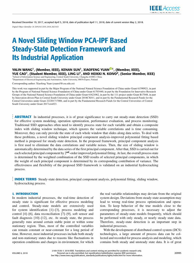
III. SLIDING WINDOW PCA-IPF BASED STEADY-STATEDETECTIONFor a single variable system, if the variable tends to be stablefor a certain period of time, the system is considered to beat steady-state, and the sampling data in this time intervalis steady-state data. As the variable data have complicatedcharacteristics like nonlinearities, a single polynomial func-tion is not sufficient to accurately model the trend of vari-able data. Sliding windows are often used to fit the wholevariable curve with piece-wise polynomials. However, as formultivariate systems, the operating variables cannot be insteady state for a long period of time in the actual industrialprocess due to switching of operation instructions and theadjustment of equipment condition. Therefore, not all thevariables can be steady, and they will vary with time to somedegree. Usually, when most of the operating variables arein steady state, the multivariate system is regarded to be atsteady state. Due to the large number of operating variables,steady-state detection of variable one by one at a time willlead to a heavy computational burden. Moreover, steady-statedetection variables are often strongly correlated as a resultof redundant sensors and mechanism relationships. Hence,before curve fitting for the trend of variable, it is necessaryto carry out dimension reduction to eliminate the redun-dant data information and capture the main data structure.PCA is able to reduce the dimension effectively and main-tain data information in the first few principal components.Hence, it is more reasonable to first carry out PCA on datato extract the main data features. Then, polynomial fittingcan be used to model the trend of each principal componentby sliding window technique. After that, steady-state indexis calculated for each principal component and a syntheticindex is obtained for steady-state detection. Fig. 1 showsthe basic flowchart of PCA-IPF based steady-state detectionmethod.

FIGURE 1. The flowchart of the proposed steady-state detectionframework.

The detailed procedure is summarized as follows:1) Assume the data series are X = [x1, . . . xi, . . . , xN ],

where xi = [xi,1, . . . , xi,j . . . , xi,M ]T . Here, N is thenumber of samples and M is the number of variablesfor steady-state detection; i and j are the sample andvariable indices, respectively.

2) For each variable j, calculate its mean value xj and stan-dard deviation δj from the observed data. Normalizeeach of the sample as follows

xi,j = (xi,j − xj)/δj (9)

Denote the data matrix after normalization asX = [x1, . . . xi, . . . , xN ].

3) Apply PCA on the normalized data matrix X, anddetermine the number D of principal components tobe kept. To select single principal component that con-tains enough information in itself, a threshold θCV forcontribution of variance is set to choose the first fewcomponents satisfying

CVd ≥ θCV , d = 1, 2, . . . ,D (10)

Then, the cumulative contribution of variance of theselected principal components is calculated to test if itis greater than the predefined threshold θCCV . If so, thenthe final number of principal components is D. if not,then new principal component is added one by one untilthe following condition is reached

CCVD ≥ θCCV (11)

where CCVD is the cumulative contribution of vari-ance for the first D principal components; θCCV isthe predefined threshold. Thus, the directions of theD principal components are p1, . . . ,pd , . . . ,pD. Then,the score of the ith sample on the d th principal directionis calculated as

zi,d = xTi pd (12)

After applying PCA on the whole dataset, we canobtain D pieces of principal component time series asz1,d , z2,d , . . . , zN ,d , (d = 1, 2, . . . ,D).

20998 VOLUME 6, 2018


4) Determine the size H of the sliding window by thefirst PC time series, which is described in detailin Section III.A.

5) Fit each selected principal component by a 2nd-orderpolynomial function with sliding window technique.The fitted time series become z1,d , z2,d , . . . , zN ,d ,(d = 1, 2, . . . ,D) for each principal component.Moreover, calculate the discriminant result of steadystate index for each PC series. Details are describedin Section III.B.

6) Compute the synthetic steady-state evaluation index bya weighted sum of the principal component indices,which are described in Section III.

A. DETERMINATION OF WINDOW SIZEThe concept of the steady-state detector [11] initially origi-nates from the theory of noise filter. As one of the simplestand most common methods, sliding window technique isoften used for steady-state detectors by analyzing statisticalcharacteristics of data. A predefined time interval is estab-lished over which the data are fitted by methods like meanfilter or polynomial function. This produces an array of fittingdata, which are much smoother than the original data. More-over, they can better represent the data trend. Hence, fittingdata in the sliding window can be used to replace each datapoint within the timespan for steady-state detection. Sincethe original data of detection variables contains noise andcorrelations, they are not suitable to be used for steady statedetection directly. In order to effectively eliminate noise indata, correlations between variables and better extract datatrend, principal components of data are used to detect steadystate by sliding window technique in this paper. To utilize thesliding window technique, the first step needed to determineis the window size. Here, a novel window size selectionmethod is adopted.

The window size is strongly related to the main data trendof steady state. Traditional methods usually determine it withcertain critical variables, which may not represent the maindata information of the steady state. To alleviate this problem,the first principal component of data is used to set the properwindow size for steady-state detection instead. As mentionedbefore, the first principal component contains the main infor-mation of data, which represents the underlying structure ofsteady-state data. Hence, it can reflect the main data trendof the process state. First, by artificially checking the timeseries of the first principal component of data, a piece ofit that remain steady are manually selected as the standardlearning time series for deciding the window size. Denotethe first PC standard learning series as zs1,1, zs2,1, . . . , zsL ,1,where L is the total number of samples in the standard series.Denote the window size is H . Therefore, the first window isconstructed and a 2nd-order polynomial function is used to fitthe first principal component data in it. After that, the windowis moved forward with step of H time intervals and the firstPC data can be fitted by the 2nd-order polynomial functionfor the second window. By sliding the window along this

TABLE 1. The procedure of determination of the window size H.

time series of the first principal component by step of Hsequentially, we can repeat this procedure until the polyno-mial fitting is finished for the first PC data of the wholestandard learning time series. Assume the time series arezs1,1, zs2,1, . . . , zsL ,1 after 2nd-order polynomial fitting withsliding windows. Then, standard deviations can be calculatedfor zs1,1, zs2,1, . . . , zsL ,1 and zs1,1, zs2,1, . . . , zsL ,1, which aredenoted δs and δs, respectively. The normalized standarddeviation is determined by

δH = δs/δs (13)

For small values of H , there are very few samples in eachwindow. Thus, a 2nd-order polynomial function is easy to beover-fitted, which will result in a large δs in the fitted standarddeviation. Too large a value of H leads to under-fitting forfirst PC data in the window. In this case, the fitted standarddeviation tends to be very small. Therefore, a reasonablevalue of H is determined by a predefined threshold of δH ,the procedure is shown in Table 1.

B. THE WINDOW FITTING AND DETECTION STRATEGYDifferent from traditional sliding window-based steady-statedetection methods, which estimate the whole window as asteady or non-steady region, the polynomial fitting approachcan evaluate the steady state for each sampling instant, whichextracts the general trend from data for steady-state detection.Hence, for each sampling instant, its state is related to thedata trend that is determined by its previous and subsequentdata. Hence, the fitting and state detection procedures foreach component are slightly different from that used in deter-mining the window size.

Here, we use z1, z2, . . . , zN to represent one general PCseries data. For each window, the data are fitted by a quadraticfunction to extract the data trend. Then, the state detectioncan be carried out for these samples in this window. However,

VOLUME 6, 2018 20999


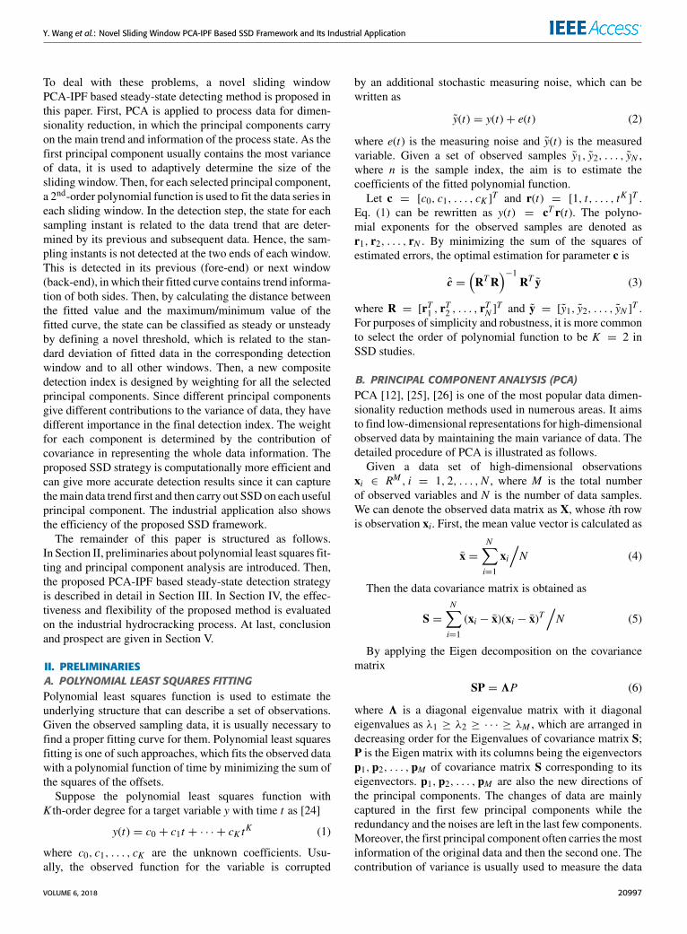
FIGURE 2. The illustration of window fitting and detection strategy.

FIGURE 3. The groups of fitted curves.

for the first and last few samples, the data trends are mainlydetermined by its latter and previous samples, respectively.This indicates that the trends of these samples are not com-pleted. Hence, for each window, only the middle parts ofsamples are detected for state. Denote the length of sampleintervals at two ends of the window as h, which usuallysatisfies h ≤ H/3. For each window, after the data are fitted,only the samples from h+ 1 to H − h are detected for steadystate. After one window is detected, it will be moved forwardbyH−2h sample intervals. Fig. 2 gives the illustration abouthow this fitting and detecting procedures are carried out.In this figure, the data in ‘‘Window n’’ are fitted by the2nd-order polynomial. Then each sample in the middle ‘‘Datan’’ of this window is detected for steady state. After that, thiswindow is forwarded byH−2h steps to get ‘‘Window n+1’’.

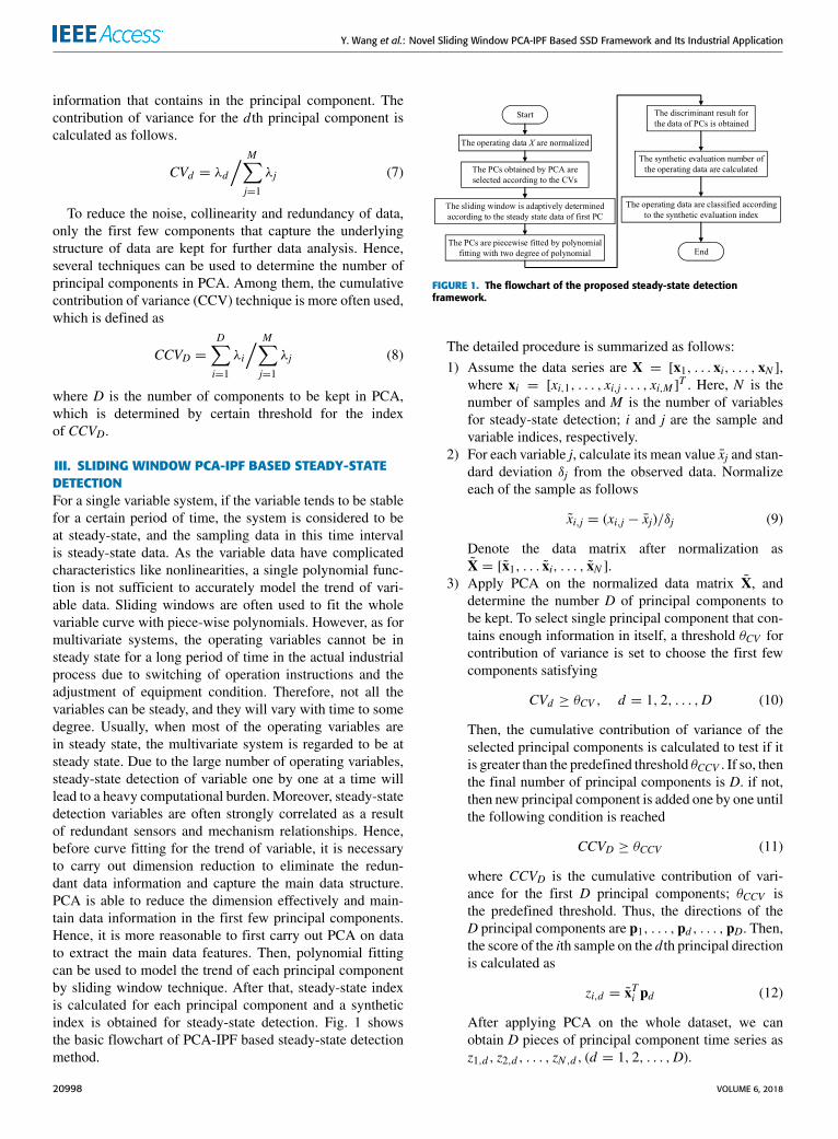
C. THE STEADY-STATE DETECTION INDEXIn the ideal case, the curve for the steady-state data should bea horizontal line because variables remain unchanged. How-ever, measured values always fluctuate due to the affectionof equipment or other conditions in real industrial processes.For each PC series, polynomial function of degree two isfitted in the sliding windows. In each window, the graphafter quadratic function fitting is a part of parabola. There aretotally six groups of fitting curves, which are shown in Fig. 3.When the size of the fitting window is the same, the more

sharply curved the graph appears, the smaller fluctuation thedata changes. Meanwhile, the fitting curve should not showa general increasing or decreasing trend, which means thatthe symmetry axis is located in the fitting curve. Moreover,the steady-state data generally fluctuates less and should beclose to the extreme value of the fitting curve. Hence, the firstgroup of fitting curves are expected to appear in practice.The second and third group curves could also exist when thereis a long period of data fluctuation. As for the fourth and fifthgroups, though the whole data trend seems to be unsteady,theremay be some steady-state data if there is short regulatingtime or measurement fluctuation. In the the last group, it iseasily seen that the process data is unsteady.

Here, 3δ rule is used to determine steady-state samples.Assume the fitting curve function for the nth window of thed th PC data series is given by

znd (t) = and t2+ bnd t + c

nd (14)

where and , bnd , c

nd are the quadratic coefficient, first-order coef-

ficient and constant term, respectively. Then the fluctuation ofthe fitted value at sampling time t to the maximum or mini-mum value of this function is calculated as

snd (t) =∣∣∣znd (t)− (4andcnd − (bnd )

2)/

4and∣∣∣ (15)

In order to identify steady and unsteady state points,the threshold for the fluctuation is defined as

θsnd = wδnd + (1− w)δd (16)

where δnd is the standard deviation of the fitted data for thed th PC in the current nth window; δd is the correspondingaverage value of standard deviations for all windows; w is theweight to control the trade-off between these two deviations.Meanwhile, to avoid misjudgment of the peak-valley datain the sixth group, standard deviation of current window isguaranteed less than a certain range.

δnd < θδnd (17)

Therefore, the steady detection index for sample at time tfrom the nth window of the d th PC series is determined as

ψnd (t) =

{1 snd (t) < 3θsnd and δ

nd < θδnd

0 else(18)

Finally, the state of the whole process is detected by thesynthetic evaluation of these principal components. As ismentioned before, different principal components providedifferent contribution of variance in representing the wholedata. Thus, a novel synthetic evaluation index is designedas the normalized sum of the evaluation index for eachcomponent

ψ(t)=D∑d=1

CVd · ψnd (t)

/ D∑d=1

CVd (19)

By predefining a threshold θψ for the synthetic eval-uation index, the process state can be classified into

21000 VOLUME 6, 2018


steady or unsteady state as

SS(t) =

{1 (steady state) ψ(t) > θψ

0 (unsteady state) otherwise(20)

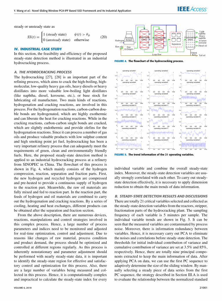
IV. INDUSTRIAL CASE STUDYIn this section, the feasibility and efficiency of the proposedsteady-state detection method is illustrated in an industrialhydrocracking process.

A. THE HYDROCRACKING PROCESSThe hydrocracking [27], [28] is an important part of therefining process, which aims to crack the high-boiling, high-molecular, low-quality heavy gas oils, heavy diesels or heavydistillates into more valuable low-boiling light distillates(like naphtha, diesel, kerosene, etc.), or base stock forlubricating oil manufacture. Two main kinds of reactions,hydrogenation and cracking reactions, are involved in thisprocess. For the hydrogenation reactions, carbon-carbon dou-ble bonds are hydrogenated, which are highly exothermicand can liberate the heat for cracking reactions. While in thecracking reactions, carbon-carbon single bonds are cracked,which are slightly endothermic and provide olefins for thehydrogenation reactions. Since it can process a number of gasoils and produce valuable products with low sulphur contentand high smoking point jet fuel, hydrocracking has been avery important refinery process that can adequately meet therequirements of green, clean and environmentally friendlyfuels. Here, the proposed steady-state detection method isapplied to an industrial hydrocracking process at a refineryfrom SINOPEC in China. The flowchart of this process isshown in Fig. 4, which mainly consists of the hydrogencompression, reaction, separation and fraction parts. First,the new hydrogen and recycled hydrogen are compressedand pre-heated to provide a continuous supply of hydrogento the reaction part. Meanwhile, the raw oil materials arefully mixed and fed to reaction part. In the reaction part, thefeeds of hydrogen and oil materials are combined to carryout the hydrogenation and cracking reactions. By a series ofcooling, heating and heat exchanges, different products canbe obtained after the separation and fraction section.

From the above description, there are numerous devices,reactions, manipulations and control strategies involved inthis complex process. Hence, a large number of processparameters and indices need to be monitored and adjustedfor real-time optimization, control and adjustment. Due toreasons like changes of raw material, process conditionand product demand, the process should be optimized andcontrolled at different regions regularly. As this process isinherently nonstationary and parameter adjustment shouldbe performed with nearly steady-state data, it is importantto identify the steady-state region for effective and satisfac-tory control and optimization for this process. Also, thereare a large number of variables being measured and col-lected in this process. Hence, it is computationally complexand impractical to calculate the steady-state index for every

FIGURE 4. The flowchart of the hydrocracking process.

FIGURE 5. The trend information of the 21 operating variables.

individual variable and combine the overall steady-stateindex. Moreover, the steady-state detection variables are usu-ally strongly correlated with each other. To carry out steady-state detection effectively, it is necessary to apply dimensionreduction to obtain the main trends of data information.

B. STEADY-STATE DETECTION RESULTS AND DISCUSSIONSThere are totally 21 critical variables selected and collected asthe steady-state detection variables from the reactors, stripper,fractionation parts of the hydrocracking plant. The samplingfrequency of each variable is 5 minutes per sample. Theindividual variable trends are shown in Fig. 5. It can beseen that the measured variables are contaminated by processnoise. Moreover, there is information redundancy betweenvariables. Hence, it is necessary carry out PCA to eliminatethe noises and correlations before steady-state detection. Thethresholds for initial individual contribution of variance andcumulative contribution of variance are set at 3.5% and 85%,respectively. Hence, there are totally nine principal compo-nents extracted to keep the main information of data. Afterapplying PCA on data, we can use the first PC sequence toadaptively determine the size of the sliding window. By man-ually selecting a steady piece of data series from the firstPC sequence, the strategy described in Section III.A is usedto evaluate the relationship between the normalized standard

VOLUME 6, 2018 21001


FIGURE 6. The relationship between the window length and thenormalized standard deviation.

FIGURE 7. The fitted results for the data of PCs.

deviation δH and the window size, which is shown in Fig. 6.From this figure, it can be seen that δH decreases sharplywhen H is small and slightly when H increases to a certainextent. Hence, the dotted line represents that the threshold ofthe normalized standard deviation is 0.7. With this threshold,the window size is determined to be 20. Then, the discardedlength of the detection is set as h = H/5 by trial and error.After the window size is determined, each of the PC series

is fitted with piecewise 2nd-order polynomial by sliding win-dow strategy as described in Section III.B. The fitting resultsof the PC data are shown in Fig.7. It can be seen that the firstPC can capture the main data information and the fitted curvereflects the smooth trend of this PC. With the increase of PCnumber, the corresponding PC occupies less data informationthan the former ones. To detect the steady-state samples foreach PC, the trade-off weight w is determined to be 0.2. Thethreshold of the standard deviation θδnd is set as 0.5.Hence, we can evaluate the steady-state index for each

sampling instant for different PCs. Then, the process

FIGURE 8. The synthetic evaluation number of the operating data.

TABLE 2. The detection results of the four methods on different datasets.

steady-state results are determined by the synthetic weightedsum of individual steady-state index for each PC. The detec-tion results are shown in Fig. 8. Here, the threshold for thesynthetic index is set as 70%, which indicates that the samplepoints above the red dot line are detected as steady state datawhile the others are unsteady state.

For performance comparison, we have further evaluatedthe proposed detection method on 6 different datasets withthree other approaches, which are the R-statistical method,PCA-IPF1 (The window is sliding forward with step one),PCA-IPF2 (with discriminant criterion from [23] and [29]).The data changes frequently in datasets 3 and 4, whiledatasets 5 and 6 have a smooth data trend. The detectionaccuracy is shown in Table 2 for the four methods on the sixdatasets. As PCA- IPF1 cannot extract the trend accuratelyat the edge of each window, its detection accuracy is lowerthan PCA-IPF. Moreover, for PCA-IPF and PCA-IPF2, IAF-PCA can provide the detection results for each sampling time,while IAF-PCA2 can only give the overall detection result forthe whole window, in which there may be both steady andunsteady points. Hence, its detection accuracy is much lowerthan PCA-IPF and PCA-IPF1. The R-statistical method givesno indication about how close the process is to the steady statebecause the detection result is only obtained by comparingthe changes in two points. Therefore, the R-statistical methodperforms a little better in test 3 and test 4, in which the processdata changes frequently. However, for the other four datasets,R-statistical method can only provide much lower accuracyof steady-state samples than PCA-IPF.

V. CONCLUSIONIn this paper, the limitations of traditional steady-state detec-tion methods are mainly focused, which usually ignore thecorrelations of variables and cannot provide accurate pointSSD result for process sampling instants. Therefore, PCA isutilized to process data for main feature extraction in orderto eliminate data correlations, redundancy and noises. Then,SSD can be carried out on the selected principal components,

21002 VOLUME 6, 2018


which can represent the main trends of process data. As thefirst principal component usually carries the most data infor-mation, it is used to determine the size of sliding window.After that, the 2nd-order polynomial is fitted for each com-ponent in the sliding windows. The fluctuation is calcu-lated between the fitted value at each sampling time and themaximum or minimum value of the fitted function. Also,the threshold is adaptively determined by the fitting functionfor all data series. By comparing the fluctuation and thethreshold, the state can be determined at different samplinginstants for each principal component. At last, the final pro-cess state is calculated by weighted sum of each principalcomponent.

REFERENCES[1] B. Jiang, F. Yang, W. Wang, and D. Huang, ‘‘Simultaneous identification

of bidirectional path models based on process data,’’ IEEE Trans. Autom.Sci. Eng., vol. 12, no. 2, pp. 666–679, Apr. 2015.

[2] X. Yuan, Y. Wang, C. Yang, Z. Ge, Z. Song, and W. Gui, ‘‘Weighted lineardynamic system for feature representation and soft sensor applicationin nonlinear dynamic industrial processes,’’ IEEE Trans. Ind. Electron.,vol. 65, no. 2, pp. 1508–1517, Feb. 2018.

[3] J. J. Shynk and N. J. Bershad, ‘‘Steady-state analysis of a single-layerperceptron based on a system identification model with bias terms,’’ IEEETrans. Circuits Syst., vol. 38, no. 9, pp. 1030–1042, Sep. 1991.

[4] X. Yuan, B. Huang, Y. Wang, C. Yang, and W. Gui, ‘‘Deep learningbased feature representation and its application for soft sensor modelingwith variable-wise weighted SAE,’’ IEEE. Trans. Ind. Informat., to bepublished, doi: 10.1109/TII.2018.2809730.

[5] A. G. Marchetti, A. Ferramosca, and A. H. González, ‘‘Steady-state targetoptimization designs for integrating real-time optimization and modelpredictive control,’’ J. Process Control, vol. 24, no. 1, pp. 129–145,2014.

[6] X. Yuan, Z. Ge, B. Huang, Z. Song, and Y. Wang, ‘‘SemisupervisedJITL framework for nonlinear industrial soft sensing based on locallysemisupervised weighted PCR,’’ IEEE Trans. Ind. Informat., vol. 13, no. 2,pp. 532–541, Apr. 2017.

[7] M. Schladt and B. Hu, ‘‘Soft sensors based on nonlinear steady-statedata reconciliation in the process industry,’’ Chem. Eng. Process., ProcessIntensification, vol. 46, no. 11, pp. 1107–1115, 2007.

[8] S. A. Bhat and D. N. Saraf, ‘‘Steady-state identification, gross error detec-tion, and data reconciliation for industrial process units,’’ Ind. Eng. Chem.Res., vol. 43, no. 15, pp. 4323–4336, 2004.

[9] M. Korbel, S. Bellec, T. Jiang, and P. Stuart, ‘‘Steady state identificationfor on-line data reconciliation based on wavelet transform and filtering,’’Comput. Chem. Eng., vol. 63, pp. 206–218, Apr. 2014.

[10] X. Yuan, Z. Ge, B. Huang, and Z. Song, ‘‘A probabilistic just-in-timelearning framework for soft sensor development with missing data,’’ IEEETrans. Control Syst. Technol., vol. 25, no. 3, pp. 1124–1132, May 2017.

[11] M. Kim, S. H. Yoon, P. A. Domanski, and W. V. Payne, ‘‘Design of asteady-state detector for fault detection and diagnosis of a residential airconditioner,’’ Int. J. Refrig., vol. 31, no. 5, pp. 790–799, 2008.

[12] X. Yuan, Z. Ge, and Z. Song, ‘‘Locally weighted kernel principalcomponent regression model for soft sensing of nonlinear time-variantprocesses,’’ Ind. Eng. Chem. Res., vol. 53, no. 35, pp. 13736–13749,2014.

[13] J. Liu,M. Gao, Y. Lv, and T. Yang, ‘‘Overview on the steady-state detectionmethods of process operating data,’’ Chin. J. Sci. Instrum., vol. 34, no. 8,pp. 1739–1748, 2013.

[14] P. Prabhakar and A. Kumar, ‘‘Performance evaluation of voltage stabilityindex to assess steady state voltage collapse,’’ in Proc. 6th IEEE PowerIndia Int. Conf., Dec. 2014, pp. 1–6.

[15] R. Dorr, F. Kratz, J. Ragot, F. Loisy, and J.-L. Germain, ‘‘Detection,isolation, and identification of sensor faults in nuclear power plants,’’ IEEETrans. Control Syst. Technol., vol. 5, no. 1, pp. 42–60, Jan. 1996.

[16] S. Narasimhan, R. S. H. Mah, A. C. Tamhane, J. W. Woodward, andJ. C. Hale, ‘‘A composite statistical test for detecting changes of steadystates,’’ AIChE J., vol. 32, no. 9, pp. 1409–1418, 1986.

[17] S. Narasimhan, S. K. Chen, and R. S. H. Mah, ‘‘Detecting changes ofsteady states using themathematical theory of evidence,’’AIChE J., vol. 33,no. 11, pp. 1930–1932, 1987.

[18] A. Maseleno and G. Hardaker, ‘‘Malaria detection using mathematicaltheory of evidence,’’ Songklanakarin J. Sci. Technol., vol. 38, no. 3,pp. 257–263, 2016.

[19] R. R. Rhinehart, ‘‘A novel method for automated identification of steady-state,’’ in Proc. Amer. Control Conf., vol. 6. Jun. 1995, pp. 4065–4066.

[20] F. Flehmig, R. V. Watzdorf, and W. Marquardt, ‘‘Identification of trends inprocess measurements using the wavelet transform,’’Comput. Chem. Eng.,vol. 22, no. 12, pp. S491–S496, 1998.

[21] T. Jiang, B. Chen, X. He, and P. Stuart, ‘‘Application of steady-statedetection method based on wavelet transform,’’ Comput. Chem. Eng.,vol. 27, no. 4, pp. 569–578, 2003.

[22] J. Wu, Y. Chen, S. Zhou, and X. Li, ‘‘Online steady-state detection forprocess control using multiple change-point models and particle filters,’’IEEE Trans. Autom. Sci. Eng., vol. 13, no. 2, pp. 688–700, Apr. 2016.

[23] K.-C. Fu, I.-K. Dai, and T.-J. Wu, ‘‘Method of adaptive steady-state detec-tion based on polynomial filtering,’’ Control Instrum. Chem. Ind., vol. 33,no. 5, p. 18, 2006.

[24] A.Marco and J.-J. Martı, ‘‘Polynomial least squares fitting in the Bernsteinbasis,’’ Linear Algebra Appl., vol. 433, no. 7, pp. 1254–1264, 2010.

[25] B. R. Bakshi, ‘‘Multiscale PCA with application to multivariate statisticalprocess monitoring,’’ AIChE J., vol. 44, no. 7, pp. 1596–1610, 1998.

[26] S. Wold, K. Esbensen, and P. Geladi, ‘‘Principal component analysis,’’Chemometrics Intell. Lab. Syst., vol. 2, nos. 1–3, pp. 37–52, 1987.

[27] J. Ancheyta, S. Sánchez, and M. A. Rodríguez, ‘‘Kinetic modeling ofhydrocracking of heavy oil fractions: A review,’’Catalysis Today, vol. 109,nos. 1–4, pp. 76–92, 2005.

[28] H. K. And and G. F. Froment, ‘‘Mechanistic kinetic modeling of thehydrocracking of complex feedstocks, such as vacuum gas oils,’’ Ind. Eng.Chem. Res., vol. 46, no. 18, pp. 5881–5897, 2006.

[29] S. Xie, C. Yang, Y. Xie, and X.Wang, ‘‘The steady state detection based onoutliers identification for sodium aluminate solution evaporation process,’’in Proc. Chin. Autom. Congr., Nov. 2015, pp. 281–285.

YALIN WANG (M’17) received the B.Eng.degree in industrial electrical automation and thePh.D. degree in control science and engineeringfrom Central South University, Changsha, China,in 1995 and 2001, respectively. She visited theUniversity of Alberta, Canada, from 2011 to 2012.She is currently a Full Professor with the Schoolof Information Science and Engineering, CentralSouth University. Her research interests includethe modeling, optimization, and control of com-

plex industrial processes, pattern recognition, and machine learning.

KENAN SUN received the B.Eng. degree in mea-surement and control technology and instrumentfrom Central South University, Changsha, China,in 2015, where he is currently pursuing the M.S.degree with the School of Information Science andEngineering. His research interests include pro-cess control and optimization, machine learning,and data mining.

XIAOFENG YUAN (M’17) received the B.Eng.and Ph.D. degrees from the Department of Con-trol Science and Engineering, Zhejiang University,Hangzhou, China, in 2011 and 2016, respectively.

He was a Visiting Scholar with the Departmentof Chemical and Materials Engineering, Univer-sity of Alberta, Edmonton, AB, Canada, from2014 to 2015. He is currently an Associate Pro-fessor with the School of Information Scienceand Engineering, Central South University. His

research interests include big data and deep learning, artificial intelligenceand machine learning, and data-driven modeling for industrial processes.

VOLUME 6, 2018 21003

http://dx.doi.org/10.1109/TII.2018.2809730


YUE CAO (S’18) received the B.Eng. degreein automation from Central South University,Changsha, China, in 2014, where he is currentlypursuing the Ph.D. degree with the School of Infor-mation Science and Engineering. His researchinterests include process monitoring, fault diagno-sis, and machine learning.

LING LI received the B.Eng. degree in automationfrom Xiangtan University in 2010 and the M.S.degree in control theory and control engineeringfrom the Nanjing University of Science and Tech-nology in 2013. She is currently pursuing the Ph.D.degree with the School of Information Science andEngineering, Central South University, Changsha,China. Her research interests include process per-formance assessment, machine learning, and datamining.

HEIKKI N. KOIVO (S’67–M’71–SM’86) receivedthe B.S.E.E. degree from Purdue University, WestLafayette, IN, USA, and the M.S. degree in elec-trical engineering and the Ph.D. degree in con-trol sciences from the University of Minnesota,Minneapolis, MN, USA. He has served in variousacademic positions at the University of Toronto,Toronto, ON, Canada, and at the Tampere Univer-sity of Technology, Tampere, Finland. Since 1995,he has been a Professor in control engineering with

the Helsinki University of Technology, Helsinki, Finland. He is a Fellow ofFinnish Academy of Technology.

21004 VOLUME 6, 2018

Documents

Wang, Yalin; Sun, Kenan; Yuan, Xiaofeng; Cao, Yue; Li