February 20, 2020

Section II Presentations

February 20, 2020

Michael Lagrange

Assistant Project Manager,

PDR Outline and Points of Failure

PDR Format and Outline: February 27th

What is Expected• Top level explanations

• Mature analysis, (Expect questions on

decision making)

What to Expect• Compile info from different sub-groups,

address sections of vehicle analysis.

Timing• ~25 – 40 min presentations

• Quick Transitions

• Ensure time for questions

Who is Presenting• PDR outline doc shows vehicle analysis

sections, one person each section

Cycler – 3:50

Tether Slings – 4:35

Mass Driver – 5:20

ED Tether – 6:10

Taxi – 6:50

Communication Satellites – 7:35

Points of Failure – Risk Analysis 1.5

Updated Key Events List Based on Changes to Mission Specifications• No longer planning to use vertical landing on mars, removed events

• Additional risk considerations to rendezvous with moving object in atmosphere

• ED tether no longer directly servicing cycler

• Etc.

Points of Failure Risk Analysis • Key Events have points of failure of highest likelihood (Mechanical or Process)

• Other points of failure are rated comparatively, severity and likelihood

• Communication with sub-groups

• Categorize using risk matrix

• Points of high severity or likelihood will require redundancy and fail-safes

Juliann Mahon

February 20, 2020Discipline: CAD Team

Vehicle and System Group: Tether Slings

ED Tether Sketches

Requirements:

Top, side, and isometric drawings of the ED

Tether in Earth Orbit

Need to Determine:

Dimensional and power requirements for the

tether

ED tether sketches sketched by Juliann Mahon

Next Steps

- Work with Power and Thermal and Structures to get accurate dimensions for the sizing of the tether.

- Create a more developed design and possible animations of the tether sling

- Work with CAD teammates on further designs of each tether

TAXI

HUB

February 20th, 2020

Dylan Pranger

Discipline: CAD

Group and System: Mass Driver

Mass Driver Design

Problem:

• Slowing down the cradle without interfering with the taxi

Old Design:

• Coil Gun

Issues:

• Could not decelerate cradle separately from taxi vehicle

• Taxi could hit coils in launch

Mass Driver Design

Design Moving Forward: Mag Lev

• Proven to work with larger loads(passenger trains)

• Solves the cradle/Taxi problem

February 20, 2020

William Sanders

Discipline: CAD

Vehicle: Taxi

Taxi Design Change

• Due to the change in our mission requirements the Taxi

design had to be significantly altered.

• The shape was changed to better manage heating due

to Martian atmospheric drag.

All Drawings and Figures by

William Sanders

Taxi Breakdown

• Still four Taxis with 24 seats each

• Passenger cabin in nose of vehicle

with two bathrooms

• Life Support, food storage, and

essential avionics located below

• Docking hatch above

• Communications Antennae in nose

cone

All Drawings and Figures by

William Sanders

February 20, 2020

Aaron Engstrom

Discipline: CAD

Vehicle and Systems Group: Cycler 14

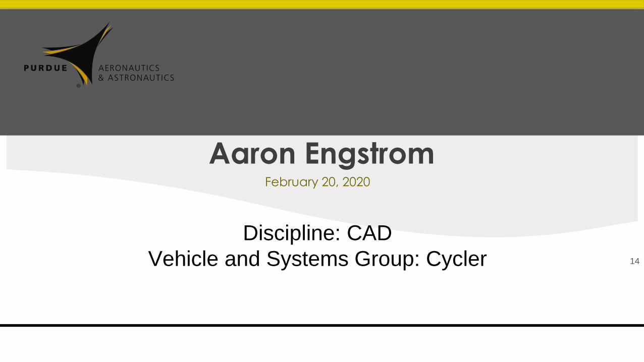
The Problem: Determine the Configuration of the Cycler Vehicle

Requirements

• Solar panels positioned to minimize solar radiation effect on Moment but also simplify

our main prop configuration

• Main prop coaxial w/ super structure, through CM

• Taxi vehicles can comfortably maneuver between the rotating elevators to the

superstructure

• HF settings modeled in the identical hab modules

Assumptions

• We are considering the average material density to be that of ISS aluminum

• Autopiloting in the future is nearly perfect when in a vacuum

Need to Determine

• Solar panel & main prop locations

• Habitation module units

15

Intermediate Design

Next Steps

• Comms modeling

• Detailed superstructure interior modeling

• Mass to be estimated once additional

materials and thicknesses are specified

• Maintain centralized dimensions document

and complete parametric modeling

16

Considerations

● 8 panels on one side is fine

○ Length perpendicular to the SS’s

longitudinal axis

● Angular velocity direction is arbitrary

● Major prop opposite the panels

● Elevator spacing has been extended

to assist with docking

vω

February 20, 2020

Nick Oetting

Communications

Communication Satellites

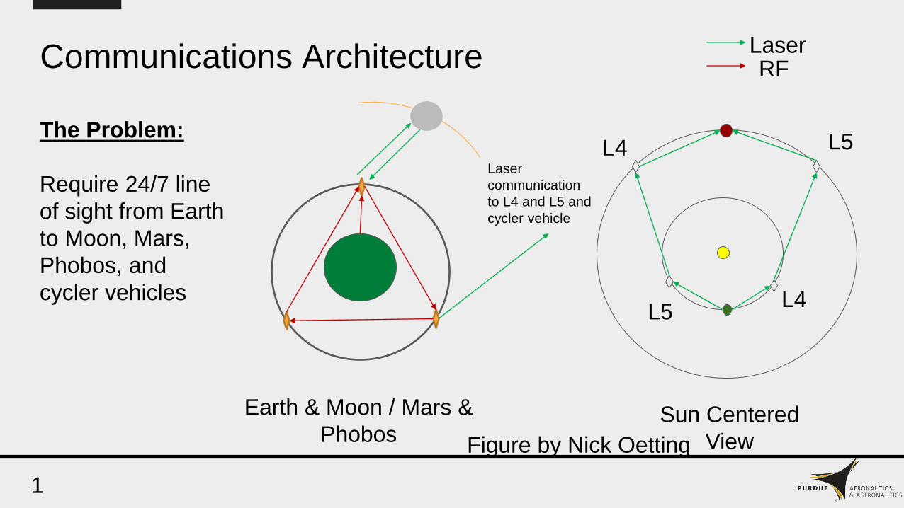
Communications Architecture

Laser

communication

to L4 and L5 and

cycler vehicle

Earth & Moon / Mars &

PhobosSun Centered

View

L5L4

L4 L5The Problem:

Require 24/7 line

of sight from Earth

to Moon, Mars,

Phobos, and

cycler vehicles

LaserRF

Figure by Nick Oetting

1

Communication System LifecycleThe Problem:

Analyze the

lifecycle of

communication

satellites at the

Lagrange points

and develop a

replacement

timeline

A 1550 nm laser has an expected lifetime of 40,000

hours ≈ 6 years [1]

Table by Nick Oetting

2

January 30, 2020

Eric Smith

Communications

Communication Satellites 20

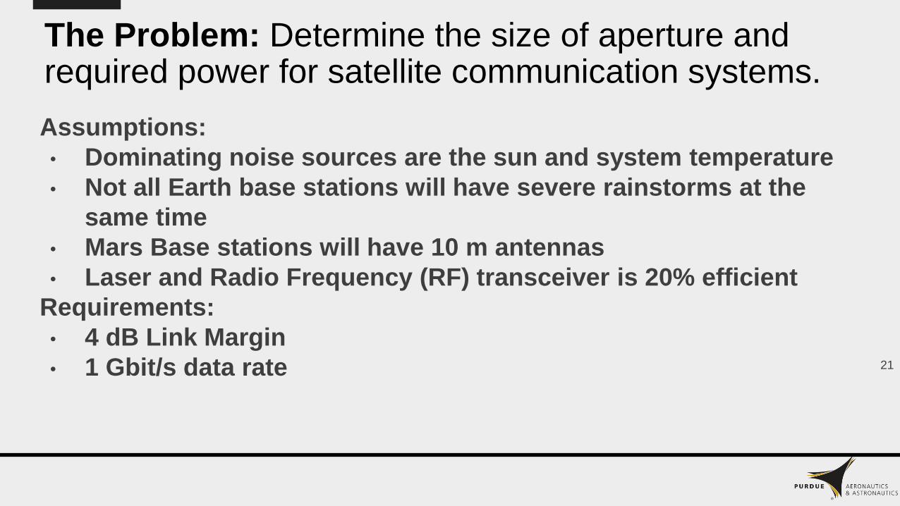
The Problem: Determine the size of aperture and required power for satellite communication systems.

Assumptions:

• Dominating noise sources are the sun and system temperature

• Not all Earth base stations will have severe rainstorms at the

same time

• Mars Base stations will have 10 m antennas

• Laser and Radio Frequency (RF) transceiver is 20% efficient

Requirements:

• 4 dB Link Margin

• 1 Gbit/s data rate 21

Solution:

22

Satellite Location Link Destination Link Type Antenna AperturePower

Required

GEO

Earth Lagrange Optical 3 m 100 W

GEO RF 2 m 500 W

Earth RF 0.5 m 250 W

Earth LagrangeMars Lagrange Optical 4 m 125 W

GEO Optical 3 m 200 W

Mars LagrangeEarth Lagrange Optical 4 m 300 W

AEO Optical 2.5 m 100 W

AEO

Mars Lagrange Optical 2.5 m 100 W

AEO RF 2 m 100 W

Mars RF 0.5 m 32.5 W

February 20th, 2020

Jacob Leet

Discipline: Controls

System: Cycler/Taxi

Problem:

Cycler Trajectory Correction:

Problem:- Investigate Trajectory changes due to

external force on the spacecraft

Requirements:- Initial positions & Velocities of Sun, Earth,

Moon, Mars, Phobos (EME2000 Frame)

- Initial position and velocity of Cycler

Assumptions:- No meteoroids hit during orbit

- No non-propulsive mass expulsion

- No effect from cosmic rays

Cycler/Taxi Interception:Problem:- Find closet location between Cycler and

Phobos for interception to minimize ΔV

- Find time range for taxi tether launch

Requirements:- Same Requirements as trajectory correction

Assumptions:- Same Requirements as trajectory correction

Model & Analysis: Orbit Simulation

Solution Method:- Initial positions & velocities of celestial bodies

retrieved from HORIZONS Web-Interface

- Initial Cycler position and velocity data retrieved

from Rob Potter’s files

Results: (Cycler #1)Trajectory offset?

There is a slight change in simulated trajectory as

compared to desired trajectory. Controller to be

introduced.

Min Distance Between Cycler and Moon:

741,600 km on December 7th, 2020

[1] Chamberlin, A. B. (n.d.). HORIZONS Web-Interface. Retrieved February 19, 2020, from

https://ssd.jpl.nasa.gov/horizons.cgi#top

[2] Longuski, J. M., Todd, R. E., & Konig, W. W. (1992). Survey of Nongravitational Forces and Space Environmental

Torques: Applied to the Galileo. Journal of Guidance, Control, and Dynamics, 15(3).

Ferbruary 20th, 2020

Yash Mishra

Controls

Feedback Control Loop to Soft-Dock the Taxi

Vehicle to the Cycler

Problem: How to achieve soft docking with the cycler

Requirements:

• Match orientation of the taxi docking port with that of the cycler

• Get taxi to match the cyclers angular velocity of 0.157 m/s

• Minimize acceleration while docking

To solve:

• Design a feedback control system for the taxi that updates its position and

orientation coordinates periodically with respect to the cycler

• Design a robotic arm for berthing the taxi into the docking port after desired

orientation has been achieved.

Solution

• Find the cycler orientation and

position in the taxi’s reference

frame

• Use taxi’s gyroscopes to get body

angles and rates and orient them

with respect to the cycler

• Introduction of a robotic arm to

match angular velocities perfectly

before soft-docking.

February 20, 2020

Kevin Huang

Mass Driver—Maximum Tolerable Acceleration

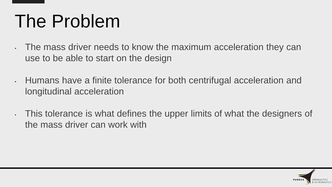
The Problem

• The mass driver needs to know the maximum acceleration they can

use to be able to start on the design

• Humans have a finite tolerance for both centrifugal acceleration and

longitudinal acceleration

• This tolerance is what defines the upper limits of what the designers of

the mass driver can work with

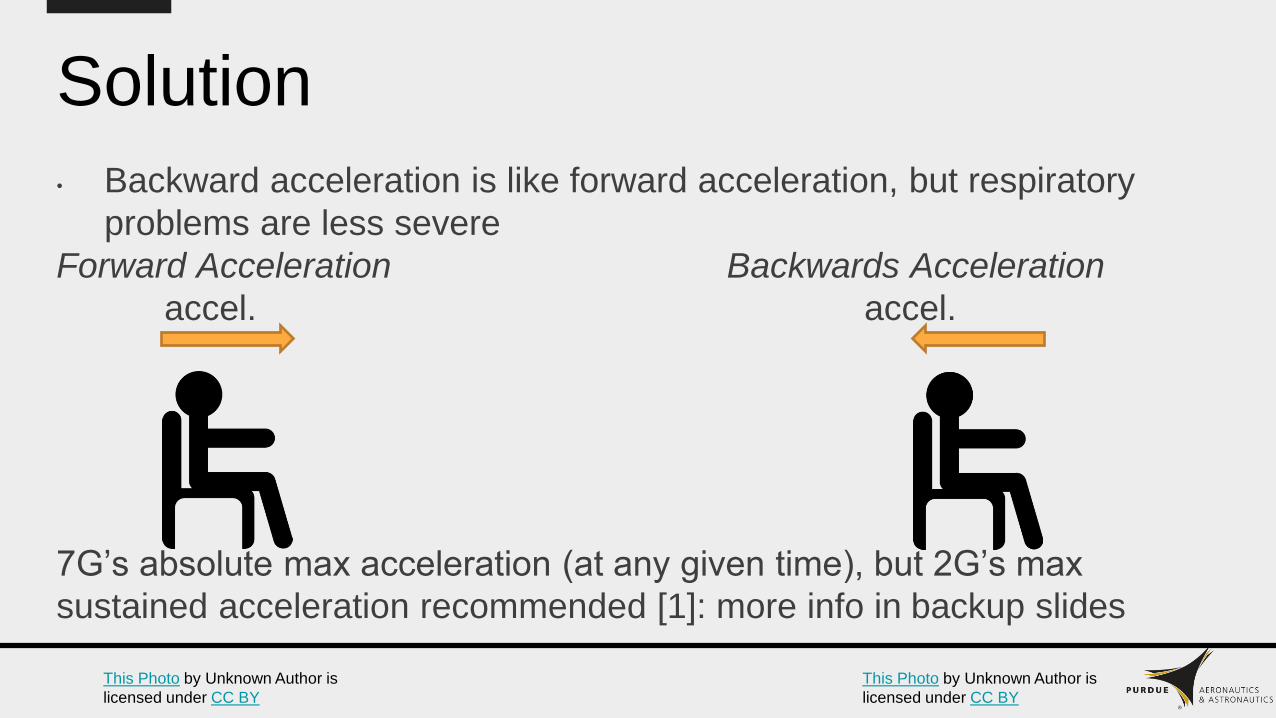
Solution

• Backward acceleration is like forward acceleration, but respiratory

problems are less severe

Forward Acceleration Backwards Acceleration

accel. accel.

7G’s absolute max acceleration (at any given time), but 2G’s max

sustained acceleration recommended [1]: more info in backup slides

This Photo by Unknown Author is

licensed under CC BY

This Photo by Unknown Author is

licensed under CC BY

February 20, 2020

Walter Manuel

Discipline: Human Factors

Vehicles/Systems: Cycler

Topic: Radiation Shielding

32

Problem: Protecting Crew from Radiation

• Space radiation is a serious threat to extended human space exploration

[1][2].

• Current NASA Exposure Limits [3]:

• Limit for radiation exposure in low-Earth orbit = 0.50 Sv/year

• Lowest career exposure limit is 1 Sv (female, 25 years old)

• Highest career exposure limit is 4 Sv (male, 55 years old)

• Maximum possible GCR exposure for 1 year [5]: 0.6 Sv

• Duration of mission: 8 months one-way, 2 years round trip

33

Solution: Aluminum Radiation Shielding

● Each trip is within NASA’s yearly exposure

limits.

● Crew members would be able to make at least

1.5 round-trips to Mars, and at most 7 round-

trips to Mars.

34

Materials Summary

● Several Materials, including polyethylene are

more effective than Aluminum.

● Heat Melt Compactor tiles are 90% as effective

as polyethylene [4].

● However, only Aluminum provides enough

structural integrity to form the outer shell.

● Multi-layered concepts have not demonstrated

significant effectiveness [9]

Material Thickness

(m)

Mass

(Mg)

Volume

(m3)

Aluminu

m

.1481 1722.6 638

Conclusions

Time

Elapsed

Effective

Dose (Sv)

8 Months .1947

1 Year .2920

2 Years .5840

February 20, 2020

Jordan Mayer

Mission Design

Communication Satellites

The Problem: Interplanetary Relay Distances and Station Keeping

● Proposal

○ 2-4 interplanetary relays at

L4/L5 Lagrange points (Sun-

Earth or Mars-Earth)

● Challenges

○ Want to minimize distances

between points of

communication

○ How much Δ𝑉 will be needed

for station keeping (SK)?

● Assumptions/Constraints

○ Assume coplanar orbits

○ Treat each system as a single

point

○ Simulate for 15 years;

geometry repeats after this

(Byrnes, Longuski, & Aldrin)

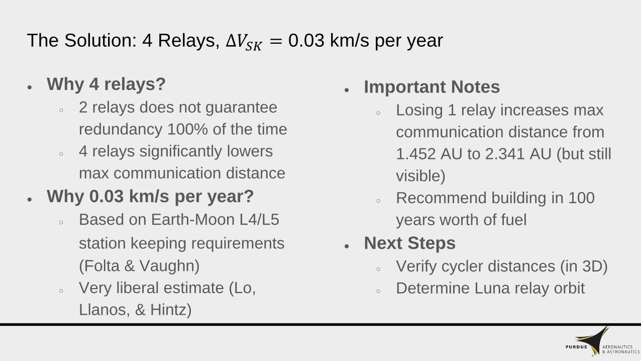
The Solution: 4 Relays, Δ𝑉𝑆𝐾 = 0.03 km/s per year

● Why 4 relays?

○ 2 relays does not guarantee

redundancy 100% of the time

○ 4 relays significantly lowers

max communication distance

● Why 0.03 km/s per year?

○ Based on Earth-Moon L4/L5

station keeping requirements

(Folta & Vaughn)

○ Very liberal estimate (Lo,

Llanos, & Hintz)

● Important Notes

○ Losing 1 relay increases max

communication distance from

1.452 AU to 2.341 AU (but still

visible)

○ Recommend building in 100

years worth of fuel

● Next Steps

○ Verify cycler distances (in 3D)

○ Determine Luna relay orbit

February 20th, 2020

Colin Miller

Mission Design (Comm Sat)

Orbital Stability Analysis at Earth and Mars

Problem

Need to Verify Relevant Forces:

• Solar Radiation Pressure (SRP)

• Third body effects

• Tesseral harmonics

• Drag

Solution Methods:

• Magnitude of gravitation at

certain points

• GMAT Simulation

Results

Drift in Degrees Per Day at Stationary:

Mars Earth

East 3.278 0.6628

Mid 1.195 0.5652

West 3.413 0.9303

Mars

:

Eart

h:

Feburary 20, 2020

Grace Ness

Mission Design:

Safe Taxi Attachment to Pre-Spun-up Tethers

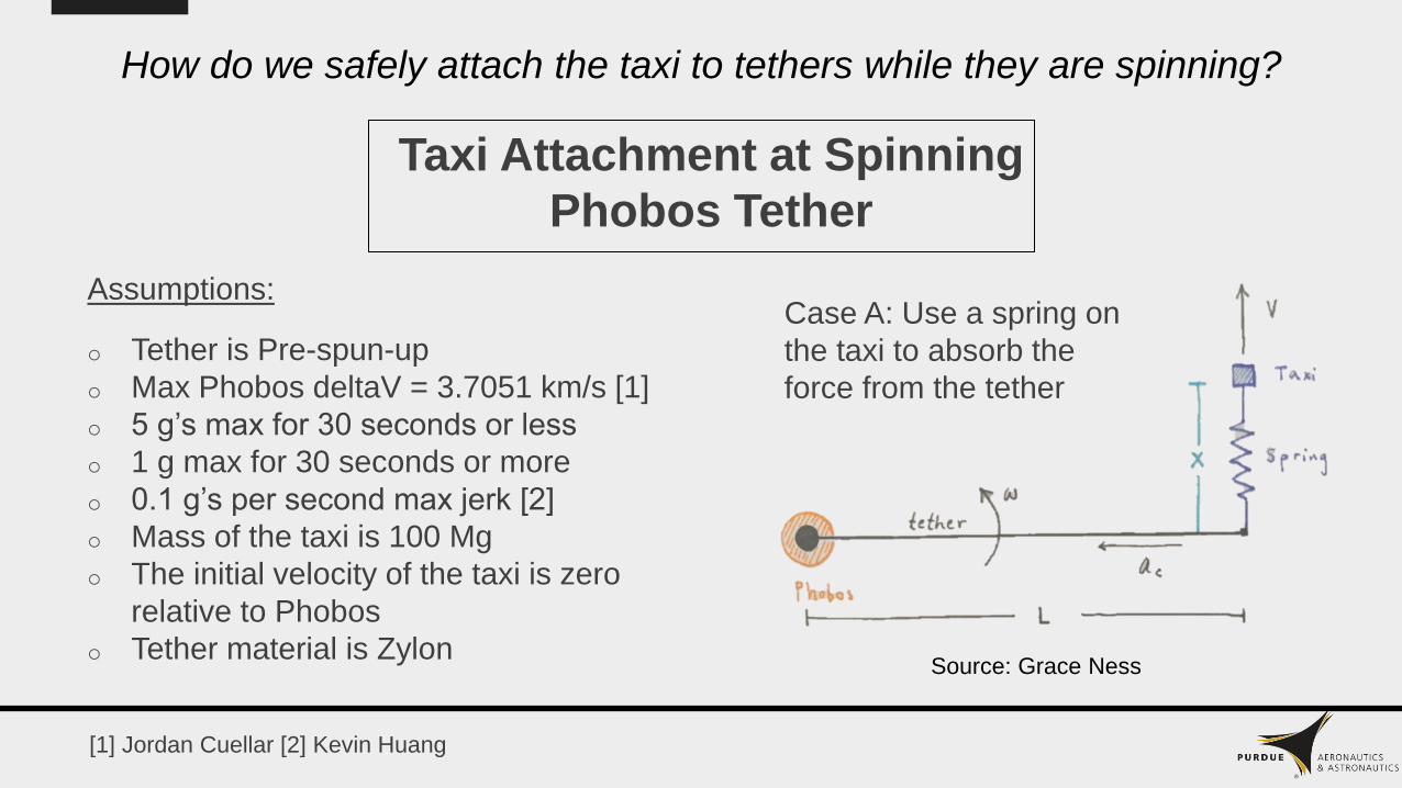
How do we safely attach the taxi to tethers while they are spinning?

Taxi Attachment at Spinning

Phobos Tether

Assumptions:

o Tether is Pre-spun-up

o Max Phobos deltaV = 3.7051 km/s [1]

o 5 g’s max for 30 seconds or less

o 1 g max for 30 seconds or more

o 0.1 g’s per second max jerk [2]

o Mass of the taxi is 100 Mg

o The initial velocity of the taxi is zero

relative to Phobos

o Tether material is Zylon

[1] Jordan Cuellar [2] Kevin Huang

Case A: Use a spring on

the taxi to absorb the

force from the tether

Source: Grace Ness

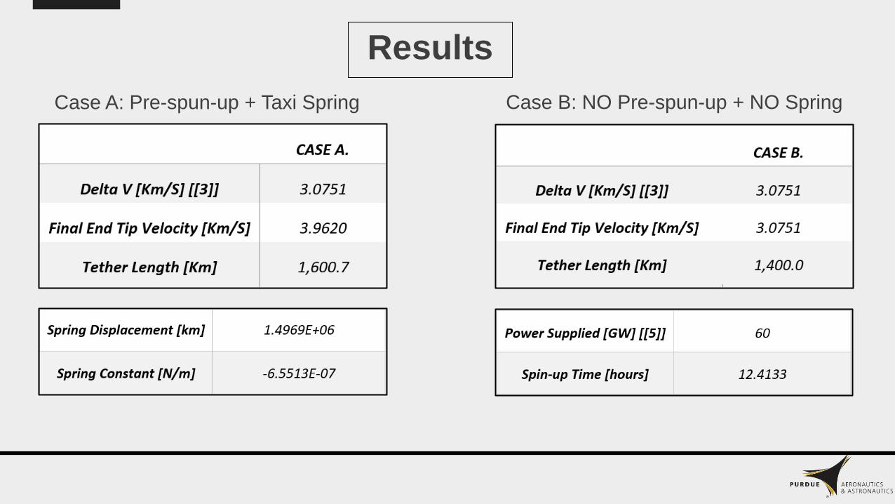
Case A: Pre-spun-up + Taxi Spring Case B: NO Pre-spun-up + NO Spring

Results

February 20, 2020

Dean Lontoc

Power and Thermal:

Taxi Vehicle Power System Configuration

Taxi Vehicle Power

[1] AAE 450: Mission Design: Jennifer Bergeson

[2] AAE 450: Structures: Nicki Liu

Presentation 1 Recap:

• Taxi needs 22kW of power.

• Chose Proton Exchange Membrane Fuel Cell (PEMFC)

Current Problem: Configure power system to last varied mission duration and withstand mission parameters [1].

Select method of reactant storage.

Fuel Cell Location in Taxi [2]

Power System Selection Matrix

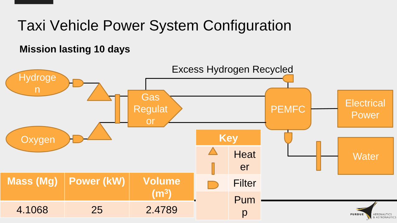
Taxi Vehicle Power System Configuration

Mass (Mg) Power (kW) Volume

(m3)

4.1068 25 2.4789

Mission lasting 10 days

Hydroge

n

Oxygen

PEMFCElectrical

Power

Water

Excess Hydrogen Recycled

Key

Heat

er

Filter

Pum

p

Gas

Regulat

or

January 30, 2020

Jacob Nunez-Kearny

Power & ThermalCycler: Power Generation & Storage

Cycler Power

Problem: Refine power generation estimates, investigate alternative power sources,

size the batteries for critical systems

Requirements:• Generate and store power for life support, communications, propulsion, etc

• Provide source of backup power for crew safety

Assumptions:• Cycler tether-spin & thermal requirements not considered

Objectives:• Refine solar panel, battery sizing for chosen TRL system

• Size alternative power source for mission-critical systems

Cycler PowerSolution:• Nominal Operation

• 1MW for propulsion, 0.85MW for life support w/ margin

• Power: 1.100 MW

• Mass: 31.51 Mg

• Surface Area: 8516 m2

• Backup life support power: Batteries vs Nuclear RTGs trade study• Batteries: 5376 MWh ➝ 1792 Mg for 10.75 Mm3

• Nuclear: 100kW ➝ 20.41 Mg for 59.48 m3

• Total mass: 54.32 Mg

Next Steps:• Perform end-of-life power calculation based on panel/mission life cycle

• Investigate power safety systems

February 20, 2020

Carly Kren

Propulsion Team

Taxi - Reaction Control Systems (RCS)

Slide: 1 of 25

The Problem: Configuration of Taxi Orbital Maneuvering System

Requirements:

• Fit in the structural allotment of 6.436m x 6.436m x 10.5m

• Achieve a minimum total ∆V = 1.529 km/sec between

each refuel• Refueling determined to be at every tether sling location

• To achieve appropriate rendezvous, orbit trajectory

transfers, and attitude adjustments of taxi

Slide: 2 of 25

*Importance of OMS

configuration on taxi*

(assume RCS thrusters

provided steering in graphic)

Destination

Well

configured

OMS

Poorly

configured

OMS

Key:

U = Ullage accounted for

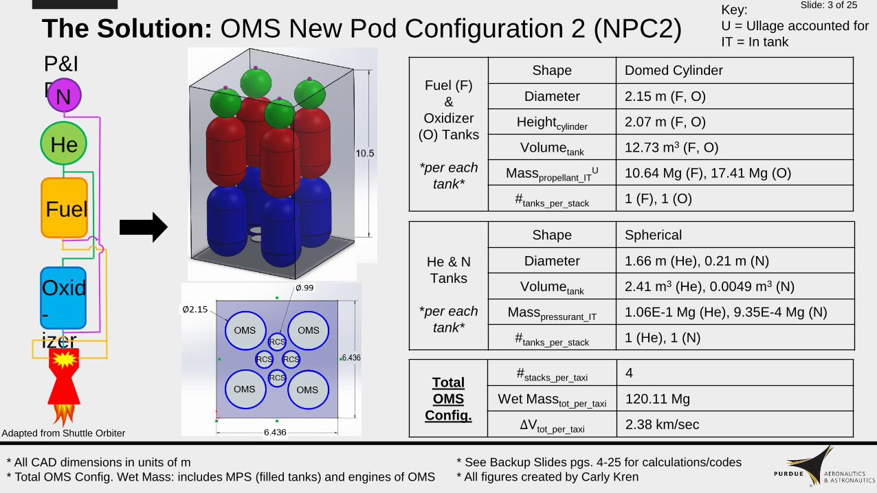
IT = In tankThe Solution: OMS New Pod Configuration 2 (NPC2)

* All CAD dimensions in units of m

* Total OMS Config. Wet Mass: includes MPS (filled tanks) and engines of OMS

P&I

D Fuel (F)

&

Oxidizer

(O) Tanks

*per each

tank*

Shape Domed Cylinder

Diameter 2.15 m (F, O)

Heightcylinder 2.07 m (F, O)

Volumetank 12.73 m3 (F, O)

Masspropellant_ITU 10.64 Mg (F), 17.41 Mg (O)

#tanks_per_stack 1 (F), 1 (O)

He & N

Tanks

*per each

tank*

Shape Spherical

Diameter 1.66 m (He), 0.21 m (N)

Volumetank 2.41 m3 (He), 0.0049 m3 (N)

Masspressurant_IT 1.06E-1 Mg (He), 9.35E-4 Mg (N)

#tanks_per_stack 1 (He), 1 (N)

Total

OMS

Config.

#stacks_per_taxi 4

Wet Masstot_per_taxi 120.11 Mg

∆Vtot_per_taxi 2.38 km/sec

Slide: 3 of 25

He

N

Fuel

Oxid

-

izer

Adapted from Shuttle Orbiter

* See Backup Slides pgs. 4-25 for calculations/codes

* All figures created by Carly Kren

February 20, 2020

Griffin Pfaff

Propulsion

Cycler - Main Propulsion System

The Problem

• Compare cryogenic propellants

to Hall Thrusters

• Minimize mass and volume

• Efficiently placed on cycler

• Accurately complete trajectory

requirements

Image by Adam Brewer

Solution

• 10 X3 Nested Hall

Thrusters[1]

• Xenon over Krypton

propellant

• Convert from liquid to

gas to minimize volume

Next Steps

• Solidify positioning on

cycler

• Calculate tank weight

and layout

Mass

(Mg)

Power

(MW)

Volume

(m^3)

Force (N)

72.58 1 23.89 54

Propellant ISP Mass (Mg)

Cryogenic[2]

(LOX/LH2)

450 397.6

X3 Nested

Hall

Thruster[1]

(Xenon)

2470 70.3

February 20, 2020

Arch Pleumpanya

Propulsion Team

Mass Driver

Problem

Cons of mass driver:

- Inefficient

- Strong and coupled magnetic fields

- Effects on humans and circuitry

Pros of maglev system:

- Mature technology [1]

- Less problem associated with coil synchronization

- Speed adjustable by frequency of AC supply

- Simple tracks

[1] Takeshita, T., Kitagawa, W., Asai, I., Nakazawa, H., & Furuhashi, Y. (2012). A museum filled with past, present and future in high speed railway -SCMAGLEV

and railway park. Journal of the Institute of Electrical Engineers of Japan, 132(10), 673-676.

Taxi vehicle

Aluminum plate

Coils

Force

Determined Parameters

- Propellant saved:

- 123 Mg at Luna

- 477 Mg at Mars

- Referring to previous presentation

- Assuming 50% of vehicle mass for

support structure

- 2 g’s acceleration limit [2]

Mars Luna

Track length

[km]

635 159

Duration [min] 4:14 2:07

Force required

[MN]

2.943 2.943

Power required

[GW]

14.72 7.37

[2] Kevin Huang, Human Factors Team

February 20, 2020

Steven Lach

Structures

Tether Sling, ED Tether, and Mass Drivers

1

The Problem: Tether Updates and Preliminary Mass Driver Sled Design

• Tether Need: Update the mass

calculations based on changes to

design

• Mass Driver Need: Initial mass

estimate and material selection for

the sled

2

Solution

Mass Driver Sled

• Material: Aluminum 6061 T6

• Mass Dependent on Taxi dimensions and

mass

Next Steps

• Run Calculations for Mars and Luna tether

slings

• Select sheath material for gondola system

• Design the hub of the tether slings with the

torque arm

• Fatigue Analysis

• Taxi Connector

3

Electrodynamic Tether

Length (km) 337

Mass (Mg) 1436

0

Cross Sectional Area at

Tip (cm2)

154

Cross Sectional Area at

Base (cm2)

654

Phobos Tether Sling

Length (km) 632

Mass (Mg) 7520

0

Cross Sectional Area at

Tip (cm2)

154

Cross Sectional Area at

Base (cm2)

2324

February 20th, 2020

Nicki (Anna) Liu

Structures

Taxi Vehicle – Stringers/Materials

Slide 1 of 3

Problem: External Loads

Slide 2 of 3

Radial Force

Requirements:

• Minimize Mass

• Prevent buckling

under

compression or

shear loads

Ribs and Stringers help to distribute load throughout

the body and reinforce the structure [1]

• Capable of carrying both tensile and compressive

loads

Radial Force

[1] Arunkumar, K. N., and Lohith, N., “Effect of Ribs and Stringer Spacings on the Weight of Aircraft Structure for Aluminum Material,” ARPN Journal of

Engineering and Applied Sciences, vol. 12, Jan. 2012, pp. 1006–1012.

• Keep skin from

bending due to

external loads

Vehicle Design

ComponentMass

(Mg)

Volume

(m3)

Available

Volume

(m3)

Needed

Support

Structure24.3 N/A N/A

Passenger

Vessel [1] [2]2.59 225 16

Cargo Vessel

[1] [2]10.1 225 80

Prop [3] 137 471 435

Total 174 921 530

[1] AAE 450: Human Factors: Emily Schott, Kait Hauber, Sarah Culp

[2] AAE 450: Power and Thermal: Dean Lontoc

[3] AAE 450: Propulsion: Carly Kren

[4] AAE 450: Human Factors: Sarah Culp

Moments of Inertia

(Mg * m2)*

Principal Moments

of Inertia (Mg * m2)*

Ixx = 1.805 * 104 Px = 267

Iyy = 1.805 * 104 Py = 620.1

Izz = 2.67 * 102 Pz = 620.5

[5] Arunkumar, K. N., and Lohith, N., “Effect of Ribs and Stringer Spacings on the Weight of Aircraft Structure for

Aluminum Material,” ARPN Journal of Engineering and Applied Sciences, vol. 12, Jan. 2012, pp. 1006–1012.

[6] Imran, M., Shi, D., Tong, L., and Waqas, H. M., “Design optimization of composite submerged cylindrical

pressure hull using genetic algorithm and finite element analysis,” Ocean Engineering

Slide 3 of 3

Rib spacing: 0.76 m

apart for 25 ribs total

Stringer spacing: 0.5 m

apart for 60 stringers total

Front View:

Figures adapted from [5],

drawn by [4]

Composite Pressure Vessel [6]

0.5 cm

0.5 cm

February 20th, 2020

Backup Slides

Slide 1 of 3

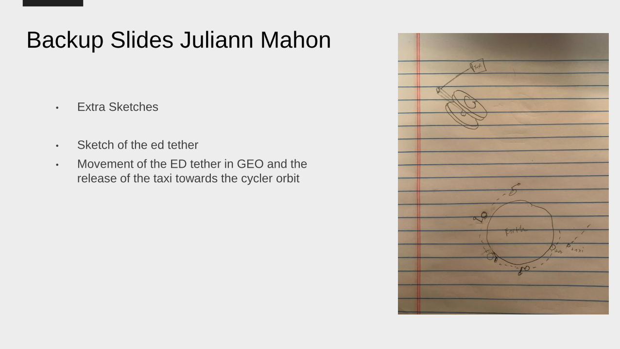
Backup Slides Juliann Mahon

• Extra Sketches

• Sketch of the ed tether

• Movement of the ED tether in GEO and the

release of the taxi towards the cycler orbit

Backup Slide 1

Chair Example

All Drawings and Figures by

William Sanders

Backup Slide 2 (previous design for reference)

All Drawings and Figures by

William Sanders

Backup Slide: Superstructure Focus

69

● The superstructure is now 60 m long (including 5 m endcaps)

● 4 docking stations

● Superstructure is motionless relative to rotating habitation modules

● 2 comms devices (location only, setup to enable continuous reception)

● 8 total minor props for controls

● 1 major prop for primary acceleration

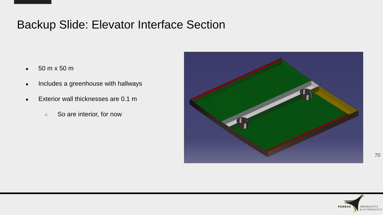
Backup Slide: Elevator Interface Section

70

● 50 m x 50 m

● Includes a greenhouse with hallways

● Exterior wall thicknesses are 0.1 m

○ So are interior, for now

Backup Slide: HAB Modules

71

● Total length: 76 m (technically an arc)

● Personal chambers (dark grey)

● Showers (cyan)

● Life support (red)

● Kitchen/commons (light grey)

● All connected by a hallway

Backup Slide: MATLAB Code for Solar Radiation Correction

72

%%%%%%%%%%%%%%%%%%%%%%%%%%%%%%%%%%%%%%%%%%%%%%%%%%%%%%%

% Aaron Engstrom | AAE 450 | Section 2 %

%%%%%%%%%%%%%%%%%%%%%%%%%%%%%%%%%%%%%%%%%%%%%%%%%%%%%%%

clear all

clc

%-----------------------------

%QUESTION:

%IS THE SOLAR PRESSURE ON THE SOLAR PANELS SIGNIFICANT ENOUGH TO AFFECT THEIR CONFIGURATION?

%THEORY:

%CALCULATE THE NECESSARY BALANCING FORCE FROM THE MINOR THRUSTERS ON THE SUPERSTRUCTURE, AND COMPARE TO CORRECTIVE ACTIONS ON THE

%I.S.S. TO JUSTIFY SIGNIFICANCE...

%CONSIDERATIONS:

%1. We round our researched values to 4 sig figs when applicable (for rapid assessment).

%2. The CM for the cycler is considered to be 2.5 m from that of the superstructure(SS), but both are still collinear with the SS longitudinal axis.

%3. Units are {[L],[M],[T]} = {[m],[kg],[s]}

%4. The SS CM is assumed to be at half its length

%5. Calculations are based on the cycler's average solar radius

Backup Slide: MATLAB Code for Solar Radiation Correction

73

%SOLUTION:

UA = 1.496 * 10^11; %standard astronomical units for Earth's average solar radius

rMarsVsUAEarth = 1.524; %ratio of Mars' average solar radius to Earth's

rMars = rMarsVsUAEarth * UA; %Mars' average solar radius

rCycler = (UA + rMars) / 2; %average solar radius of the cycler

PSun = 3.8 * 10^26; %average power output by the Sun (in kg*m^2/s^3)

A = 13440; %solar paneling surface area (1 side) obtained from Jacob Nunez

c = 2.998 * 10^8; %speed of light

ISun = PSun / (4 * pi * rCycler ^ 2); %intensity of solar radiation

p = 2 * ISun / c; %surface pressure due to solar radiation

Fduetop = p * A; %force due to solar radiation pressure over one second

solarPanelW = 16.8; %solar panel width (length is 100 m)

solarPanelSep = .1; %estimate separation between panels or the first panels and end cap

SSLength = 45; %length of the superstructure

CMOffset = 2.5; %Cycler CM offset from SS CM

lengthCyclerCMtoCap = SSLength / 2 - CMOffset; %length from the solar panel mounting cap to the Cycler CM

Fduetopr = 2 * solarPanelW + 2 * solarPanelSep + lengthCyclerCMtoCap; %applicable radius for solar pressure on the moment about CM

minorPropSep = 1.5; %distance from minor prop axis' to end cap

minorPropr = SSLength - lengthCyclerCMtoCap - minorPropSep;

radiiRatio = Fduetopr / minorPropr;

balT = Fduetop * radiiRatio; %required balancing thrust

% Through simple anaylsis... by comparing our balT value (which is 0.1741 kg*m/s/s), that is the necessary balancing thrust from the minor props, to values for re-boosting

% on the I.S.S. to correct for atmospheric drag (which is 0.275 N for one second applied to a space-craft that is half as massive)... we can see that the torque about the CM

% of the cycler is insignificant.

%ANSWER:

%NO

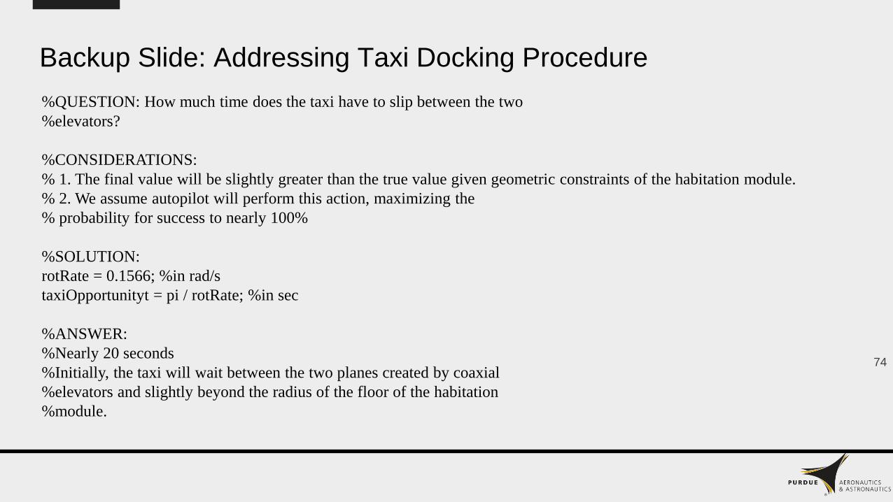
Backup Slide: Addressing Taxi Docking Procedure

74

%QUESTION: How much time does the taxi have to slip between the two

%elevators?

%CONSIDERATIONS:

% 1. The final value will be slightly greater than the true value given geometric constraints of the habitation module.

% 2. We assume autopilot will perform this action, maximizing the

% probability for success to nearly 100%

%SOLUTION:

rotRate = 0.1566; %in rad/s

taxiOpportunityt = pi / rotRate; %in sec

%ANSWER:

%Nearly 20 seconds

%Initially, the taxi will wait between the two planes created by coaxial

%elevators and slightly beyond the radius of the floor of the habitation

%module.

References

Petty, J. I., “STS-113 Payloads,” National Aeronautics and Space Administration,

Oct. 2002.

“Reference Guide to the International Space Station,” National Aeronautics and

Space Administration, Sep. 2015.

“Shreve Room Layout,” Housing at Purdue University Available:

https://www.housing.purdue.edu/Housing/Residences/Shreve/layout.html.

75

References

[1] – Hamid Hemmati, Deep Space Optical Communications, Jet Propulsion

Laboratory, California Institute of Technology, Pasadena, CA, 2005, pp. 336

[2] - Shiotani, Bungo & Fitz-Coy, Norman & Asundi, Sharan. (2014). An End-to-

End Design and Development Life-Cycle for CubeSat class Satellites.

10.2514/6.2014-4194.

3

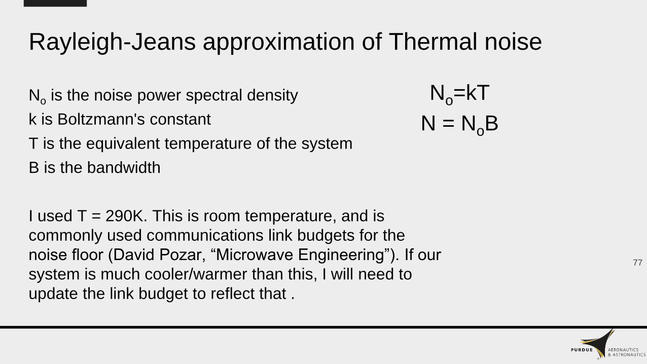
Rayleigh-Jeans approximation of Thermal noise

No is the noise power spectral density

k is Boltzmann's constant

T is the equivalent temperature of the system

B is the bandwidth

I used T = 290K. This is room temperature, and is

commonly used communications link budgets for the

noise floor (David Pozar, “Microwave Engineering”). If our

system is much cooler/warmer than this, I will need to

update the link budget to reflect that .

77

No=kT

N = NoB

Solar NoiseOptical System Noise

• The solar irradiance at 1550 nm is 0.3 W/(m2 nm) at 1 AU (Thuillier, G. “The Solar Spectral

Irradiance from 200 to 2400 nm”).

• The power follows an inverse square law, so at Mars, which has an orbital radius of 1.53 AU, the

solar irradiance at 1550 nm will be 0.3*(12/1.532) W/(m2 nm) which is ~0.128 W/(m2 nm).

• The power of the solar light is added to the power of the thermal noise power to estimate the total

noise in the optical systems.

RF System Noise

• In Ka-Band, the sun has an equivalent temperature of 6000K (Ho, C. “Solar Brightness Temperature

and Corresponding Antenna Noise Temperature at Microwave Frequencies”). The noise power

spectral density is then determined via the Rayleigh-Jeans approximation to be ~8.3x10-20 W/Hz

• This power is added to the thermal noise power of the system to estimate the total noise of the RF

systems. 78

Atmospheric Loss

For Ka-Band, typical atmospheric losses for Earth are ~4 dB but can be as

high as 50 dB in rare cases (~0.001% of the time) of large storms (Hemmati,

H., “Deep Space Optical Communications,”). My link budget accounts for the

4 dB case. For our system to deal with the extreme case, the link can be

completed by communicating with one of the other GEO satellites that have a

clear connection, or increase the number of receivers on Earth to decrease

the chance that they all will be in a storm.

At Mars, atmospheric losses are low, except in the case of dust storms. Even

in this extreme case, however, the loss of Ka-Band signals is ~3.4 dB

(Hemmati, H., “Deep Space Optical Communications,”). I account for this

worse case scenario since developing more infrastructure on Mars would be

more difficult than dealing with the extra 3 dB of loss.

79

Satellite Overview

80

GEO Satellites

● 3m

telescope

(to/from

Earth

Lagrange)

● 2x 2m

cross-link

antenna

● 0.5m

downlink

antenna

AEO Satellites

● 2.5m

telescope

(to/from

Mars

Lagrange)

● 2x 2m

cross-link

antenna

● 0.5m

downlink

antenna

Mars Lagrange

Satellites

● 2.5m

telescope

(to/from AEO)

● 4m telescope

(to/from Mars

Lagrange)

Earth Lagrange

Satellites

● 3m

telescope

(to/from

GEO)

● 4m

telescope Illustration by Eric

Smith

References

[1] Pozar, D. M., “Microwave Engineering”, Noise and Nonlinear Distortions, 4th edition., Wiley,

Hoboken, NJ, 2012.

[2]Thuillier, G., Hersé, M., Labs, D., Foujols, T., Peetermans, W., Gillotay, D., Simon, P., and

Mandel, H., “The Solar Spectral Irradiance from 200 to 2400 nm as Measured by the SOLSPEC

Spectrometer from the Atlas and Eureca Missions,” Solar Physics, Vol. 214, No. 1, ????, pp. 1–22.

https://doi.org/10.1023/A:1024048429145.

[3]Hemmati, H., “Deep Space Optical Communications,”Deep Space Optical Communications,

2006, pp. 1–705. https://doi.org/10.1002/0470042419.

[4]Ho, C., Slobin, S., Kantak, A., and Asmar, S., “Solar Brightness Temperature and Corresponding

Antenna Noise Temperature at Microwave Frequencies,”The Interplanetary Network . . ., 2008, pp.

1–11. URL http://ipnpr.jpl.nasa.gov/progress{_}report/42-175/175E.pdf

81

February 20, 2020

Kevin Huang

Presentation 2 Backup Slides

Sources

[1] Kumar, K. V., and Norfleet, W. T., “NASA Technical Reports Server

(NTRS)2008364NASA Technical Reports Server (NTRS). Washington, DC:

NASA Center for Aerospace Information Last visited June 2008. Gratis URL:

http://ntrs.nasa.gov/,” Issues on Human Acceleration Tolerance After Long-

Duration Space Flights, Oct. 1992, pp. 12–24.

Effects of Multiple G’s on HumansForward

Linear/Longitudinal

Acceleration

(+Gx): acceleration

one would

experience in a car

Table created from

Source [1]

G’s

experien

ced

Effects G’s

experienc

ed

1 breathing starts

quickening

2 dizziness; tolerable

up to 24 hours8

3-6 tightness in chest,

difficulty breathing,

shortness of breath,

blurring of vision,

difficulty speaking,

potentially

dangerous increase

in heartrate

9-12 breathing

becomes very

hard due to

pressure

imbalance in

lungs (blood

rushes to back of

chest)--decreased

oxygen delivery

7 UPPER LIMIT >12 pain in the chest;

loss of vision

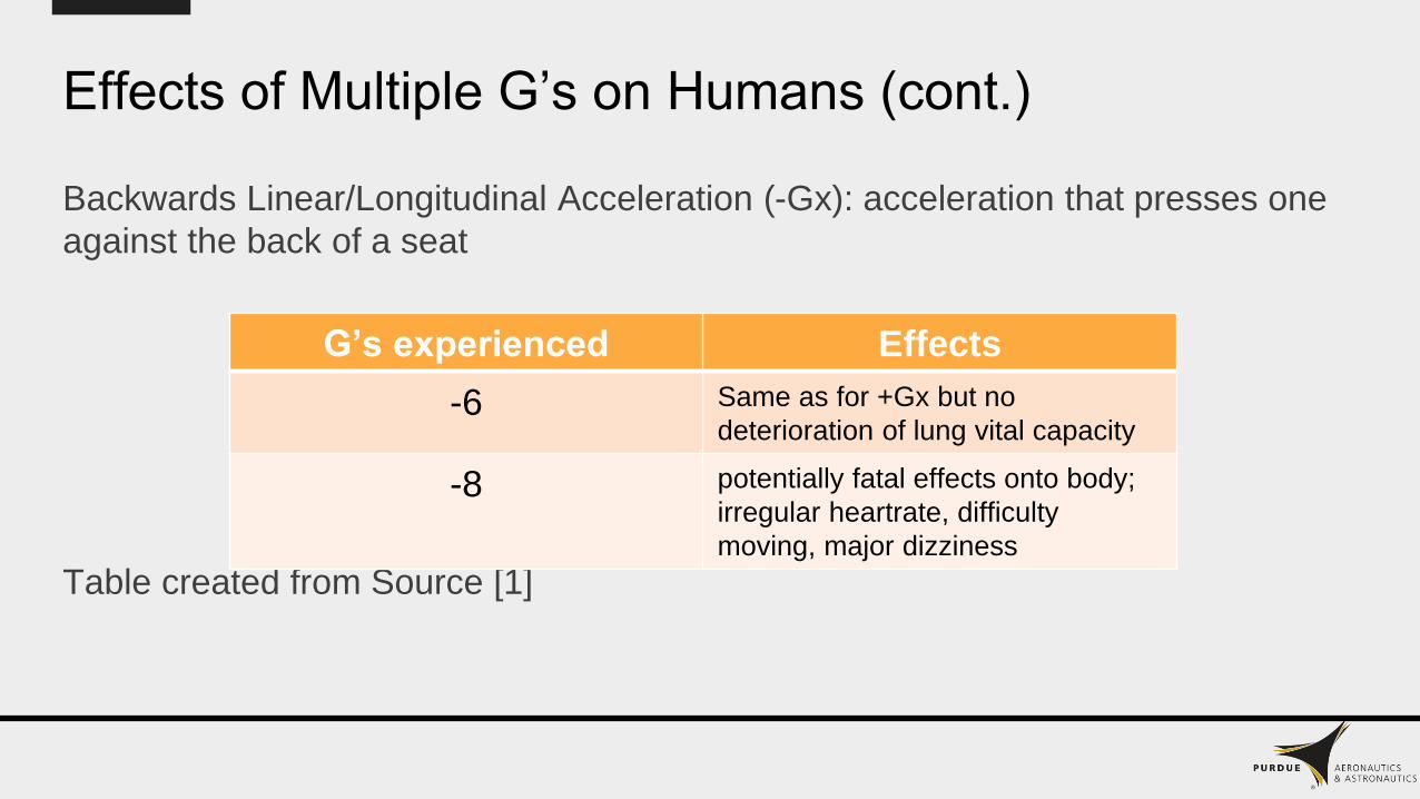
Effects of Multiple G’s on Humans (cont.)

Backwards Linear/Longitudinal Acceleration (-Gx): acceleration that presses one

against the back of a seat

Table created from Source [1]

G’s experienced Effects

-6 Same as for +Gx but no

deterioration of lung vital capacity

-8 potentially fatal effects onto body;

irregular heartrate, difficulty

moving, major dizziness

Effects of Multiple G’s on Humans (cont.)

While it was recommended that 2G’s was used, it is acceptable to use 3-4 G’s if it

is acceptable for the customers to experience discomfort for a while; the more

dangerous side-effects noted in previous slides are only relevant for people

already dispositioned to heart issues on top of the fact that they only start to get

relevant for the higher G’s

During Launch

Humans are more resilient to Gx accel. than centrifugal acceleration (Gz; gravity

is a form of Gz acceleration); therefore, for launch, recommend inclining seats to

reduce Gz vector and increase Gx vector

--Effective Physiologic Angle, or EPA [angle between acceleration vector and line

of spacecraft]: recommended to be between 8 to 12 degrees [1]

Linear Accelerations: Peak G’s experienced vs recommended maximum duration

G-Axis

Peak G's

Experienced

Time before

blackout (sec)

+Gz 12 0.04

5 0.1

3 180

-Gz 6 0.02

5 0.1

2 30

+Gx 25 0.04

15 0.2

8 150

-Gx 25 0.04

15 0.2

6 60

January 30, 2020

Walter Manuel – Backup Slides

Discipline: Human Factors

Vehicles/Systems: Cycler

Topic: Radiation Shielding

89

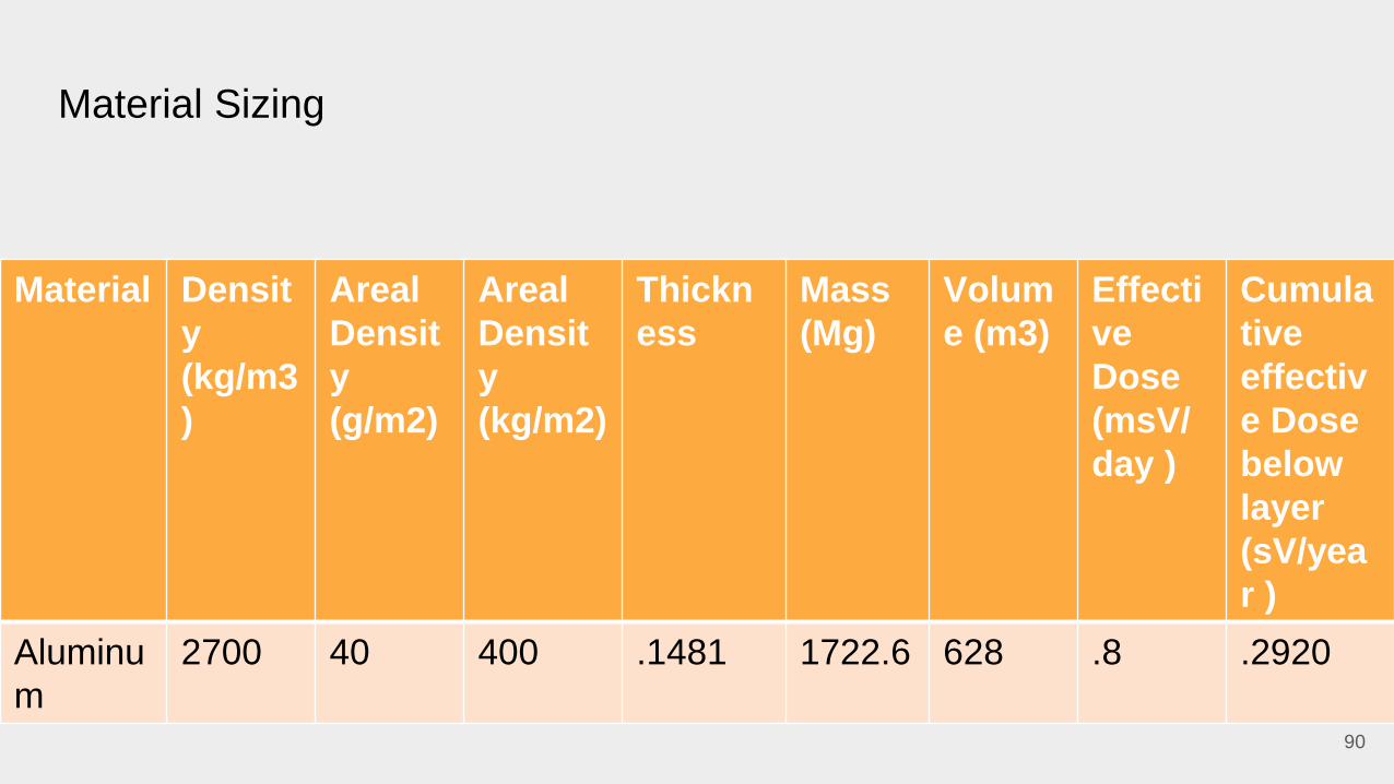
Material Sizing

90

Material Densit

y

(kg/m3

)

Areal

Densit

y

(g/m2)

Areal

Densit

y

(kg/m2)

Thickn

ess

Mass

(Mg)

Volum

e (m3)

Effecti

ve

Dose

(msV/

day )

Cumula

tive

effectiv

e Dose

below

layer

(sV/yea

r )

Aluminu

m

2700 40 400 .1481 1722.6 628 .8 .2920

Solar Particle Event Shielding Option

● “Storm Shelter” – Can be formed by reorganizing supplies or by having a designated area [6]

● Protective vests [7]

● Early warning and detection systems (EWDS) [8]

● Protective vests, used in conjunction with EWDS, were chosen as the solution to best protect the

crew from Solar Particle Events. During times of peak radiation, crew members will receive warning

and can don their protective vests. These protective vests are made of a combination of polyethylene

and are relatively thin, akin to a jacket. As a result, their mass is negligible, so they can be factored into

the mass and volume calculations as included in the crew personal belongs and articles of clothing.

References[1] https://www.nasa.gov/feature/goddard/2019/how-nasa-protects-astronauts-from-space-radiation-at-moon-mars-solar-cosmic-rays

[2 ]https://www.nasa.gov/feature/goddard/real-martians-how-to-protect-astronauts-from-space-radiation-on-mars

[3] NASA. (2008). The Radiation Challenge.

https://www.nasa.gov/pdf/284273main_Radiation_HS_Mod1.pdf

[4] Rais-Rohani, M. (2004). On Structural Design of a Mobile Lunar Habitat with Multi-Layered

Environmental Shielding. Retrieved from NASA Faculty Fellowship Program website:

https://ntrs.nasa.gov/archive/nasa/casi.ntrs.nasa.gov/20050215340.pdf

[5] Bahadori, A., Semones, E., Ewert, M., Broyan, J., & Walker, S. (2017). Measuring space

radiation shielding effectiveness. EPJ Web of Conferences, 153, 04001.

doi:10.1051/epjconf/201715304001

[6] Mary Beth Griggs. (2016, September 23). This Is How Orion Astronauts Might Protect Themselves From

Radiation Storms. Retrieved from https://www.popsci.com/this-is-how-orion-astronauts-might-protect-

themselves-from-radiation-storms/

[7] Lockheed Martin. (n.d.). How a Wearable Vest Can Protect Astronauts on a Mission to

Mars. https://www.lockheedmartin.com/en-us/news/features/2016/stemrad-vest-space.html

[8 ]https://three.jsc.nasa.gov/articles/Shielding81109.pdf

[9] Li, X., Warden, D., & Bayazitoglu, Y. (2018). Analysis to Evaluate Multilayer Shielding of

Galactic Cosmic Rays. JOURNAL OF THERMOPHYSICS AND HEAT TRANSFER, 32(2).

Retrieved from DOI: 10.2514/1.T5292

92

February 20, 2020

Jordan Mayer

Mission Design

Communication Satellites

Backup Slides

Appendix A: References

1. Byrnes, D. V., Longuski, J. M., and Aldrin, B., “Cycler Orbit Between

Earth and Mars,” Journal of Spacecraft and Rockets, Vol. 30, No. 3,

1993, pp. 334-336.

2. Folta, D., and Vaughn, F., “A Survey of Earth-Moon Libration Orbits:

Stationkeeping Strategies And Intra-Orbit Transfers,” AIAA Paper

2004-4741, August 2004.

3. Lo, M., Llanos, P, and Hintz, G., “An L5 Mission to Observe the Sun

And Space Weather, Part 1,” AAS Paper 10-121, February 2010.

4. Williams, D., “Sun Fact Sheet,” Planetary Fact Sheet, NASA

Goddard Space Flight Center, retrieved 10 February 2020.

https://nssdc.gsfc.nasa.gov/planetary/factsheet/sunfact.html

5. Williams, D., “Earth Fact Sheet,” Planetary Fact Sheet, NASA

Goddard Space Flight Center, retrieved 10 February 2020.

https://nssdc.gsfc.nasa.gov/planetary/factsheet/earthfact.html

Appendix A: References

6. Williams, D., “Mars Fact Sheet,” Planetary Fact Sheet, NASA

Goddard Space Flight Center, retrieved 10 February 2020.

https://nssdc.gsfc.nasa.gov/planetary/factsheet/marsfact.html

NOTE: Williams not referenced in slides, but used to obtain necessary

values for orbit prediction

Appendix B: MATLAB Code

NOTE: The function kep2car.m was created by Dr. Carolin Frueh of

Purdue University, and is used with her permission. All other code was

created by Jordan Mayer.

Appendix B: MATLAB Code%%%%%

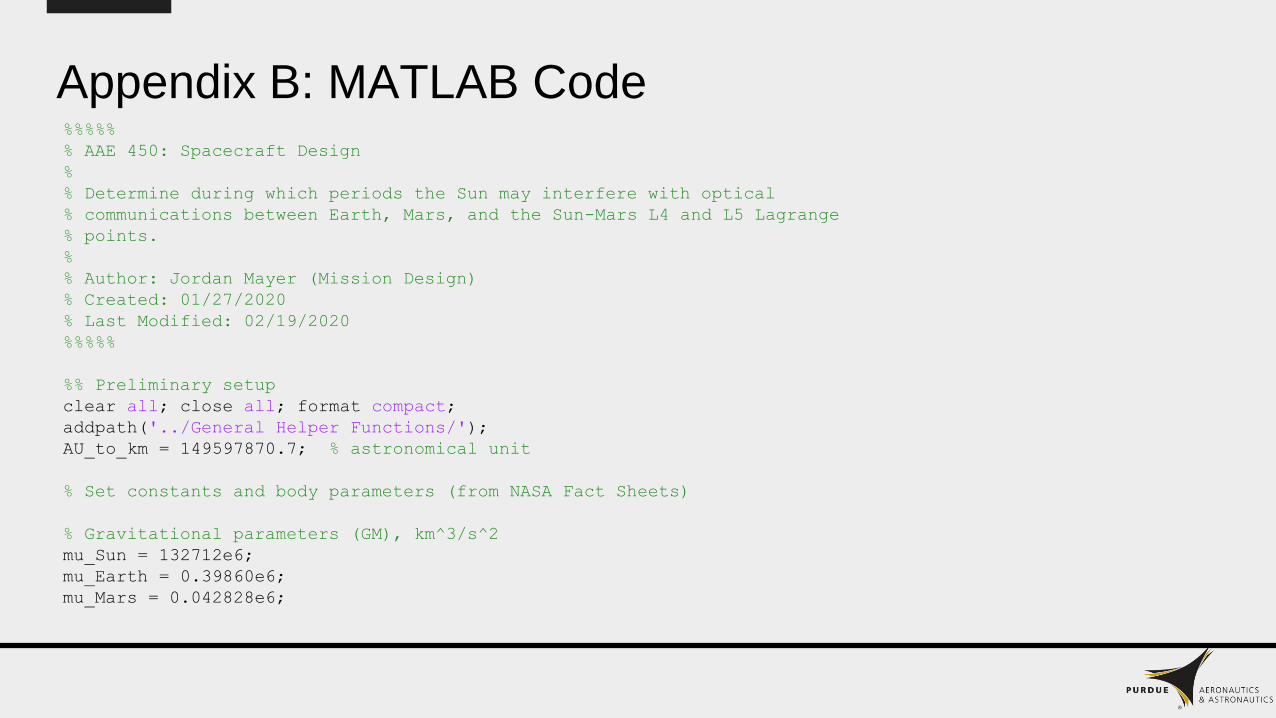
% AAE 450: Spacecraft Design

%

% Determine during which periods the Sun may interfere with optical

% communications between Earth, Mars, and the Sun-Mars L4 and L5 Lagrange

% points.

%

% Author: Jordan Mayer (Mission Design)

% Created: 01/27/2020

% Last Modified: 02/19/2020

%%%%%

%% Preliminary setup

clear all; close all; format compact;

addpath('../General Helper Functions/');

AU_to_km = 149597870.7; % astronomical unit

% Set constants and body parameters (from NASA Fact Sheets)

% Gravitational parameters (GM), km^3/s^2

mu_Sun = 132712e6;

mu_Earth = 0.39860e6;

mu_Mars = 0.042828e6;

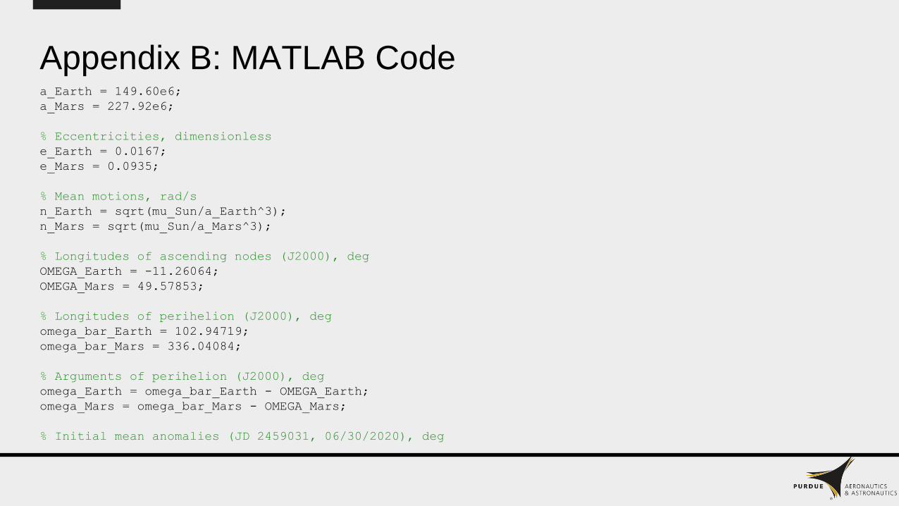
Appendix B: MATLAB Code% Semimajor axes, km

a_Earth = 149.60e6;

a_Mars = 227.92e6;

% Eccentricities, dimensionless

e_Earth = 0.0167;

e_Mars = 0.0935;

% Mean motions, rad/s

n_Earth = sqrt(mu_Sun/a_Earth^3);

n_Mars = sqrt(mu_Sun/a_Mars^3);

% Longitudes of ascending nodes (J2000), deg

OMEGA_Earth = -11.26064;

OMEGA_Mars = 49.57853;

% Longitudes of perihelion (J2000), deg

omega_bar_Earth = 102.94719;

omega_bar_Mars = 336.04084;

% Arguments of perihelion (J2000), deg

omega_Earth = omega_bar_Earth - OMEGA_Earth;

omega_Mars = omega_bar_Mars - OMEGA_Mars;

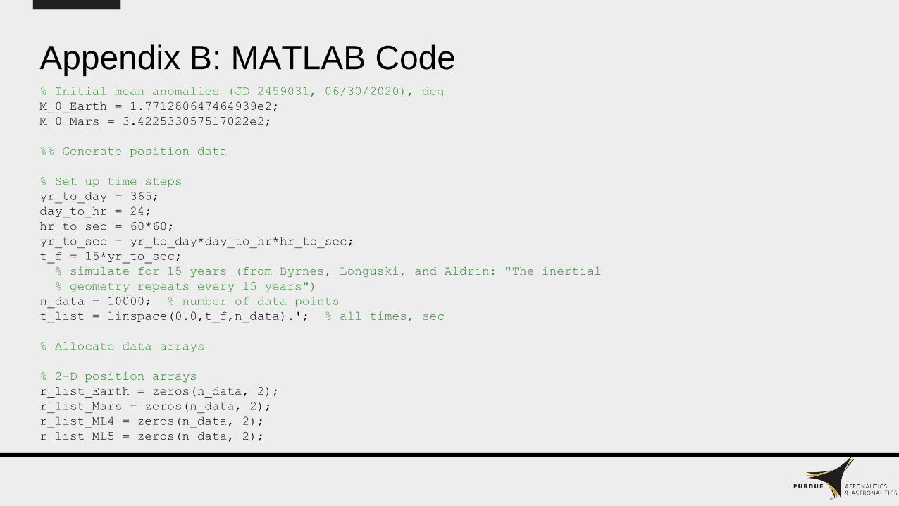
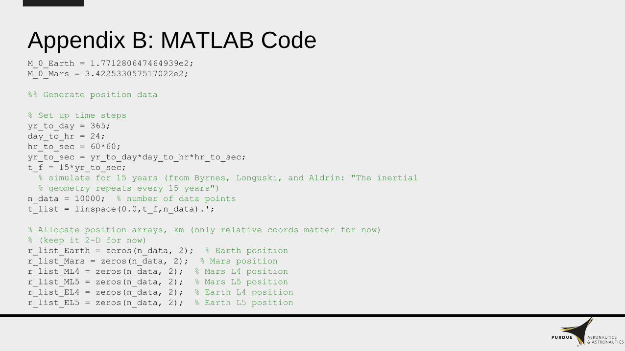
Appendix B: MATLAB Code% Initial mean anomalies (JD 2459031, 06/30/2020), deg

M_0_Earth = 1.771280647464939e2;

M_0_Mars = 3.422533057517022e2;

%% Generate position data

% Set up time steps

yr_to_day = 365;

day_to_hr = 24;

hr_to_sec = 60*60;

yr_to_sec = yr_to_day*day_to_hr*hr_to_sec;

t_f = 15*yr_to_sec;

% simulate for 15 years (from Byrnes, Longuski, and Aldrin: "The inertial

% geometry repeats every 15 years")

n_data = 10000; % number of data points

t_list = linspace(0.0,t_f,n_data).'; % all times, sec

% Allocate data arrays

% 2-D position arrays

r_list_Earth = zeros(n_data, 2);

r_list_Mars = zeros(n_data, 2);

r_list_ML4 = zeros(n_data, 2);

r_list_ML5 = zeros(n_data, 2);

Appendix B: MATLAB Coder_list_EL4 = zeros(n_data, 2);

r_list_EL5 = zeros(n_data, 2);

% Visibility arrays (0 if visible, 1 if not)

% ML: Mars-Sun Lagrange point

% EL: Earth-Sun Lagrange point

ML4_block_list = zeros(n_data, 1);

ML5_block_list = zeros(n_data, 1);

Mars_block_list = zeros(n_data, 1);

EL4_block_list = zeros(n_data, 1);

EL5_block_list = zeros(n_data, 1);

% Minimum distance arrays

min_dist_Earth_ML = zeros(n_data, 1); % Earth to closest ML4/ML5

min_dist_Mars_EL = zeros(n_data, 1); % Mars to closest EL4/EL5

min_dist_EL_ML = zeros(n_data, 1);

% Shortest distance between EL4/EL5 and ML4/ML5

% Prepare Keplerian element arrays

% [semimajor axis (km), eccentricity, inclination (deg), longitude of

% ascending node (deg), argument of periapsis (deg), mean anomaly (deg)]

kep_Earth = [a_Earth, e_Earth, 0.0, OMEGA_Earth, omega_Earth, M_0_Earth];

kep_Mars = [a_Mars, e_Mars, 0.0, OMEGA_Mars, omega_Mars, M_0_Mars];

Appendix B: MATLAB Code% Compute position data

for k = 1:n_data

delta_t = t_list(k);

% Compute mean anomalies, deg

M_Earth = M_0_Earth + rad2deg(n_Earth*delta_t);

M_Mars = M_0_Mars + rad2deg(n_Mars*delta_t);

% Update Keplerian element arrays

kep_Earth(6) = M_Earth;

kep_Mars(6) = M_Mars;

% Compute Cartesian vectors [position (km), velocity (km)]

car_Earth = kep2car(kep_Earth, mu_Sun, 'deg');

car_Mars = kep2car(kep_Mars, mu_Sun, 'deg');

if car_Earth(3) > 0 || car_Mars(3) > 0

error('3-D?');

end

% Get 3-D position vectors

r_Earth = car_Earth(1:3);

r_Mars = car_Mars(1:3);

r_ML4 = rot_mat_3(deg2rad(60)) * r_Mars;

Appendix B: MATLAB Coder_ML5 = rot_mat_3(deg2rad(-60)) * r_Mars;

r_EL4 = rot_mat_3(deg2rad(60)) * r_Earth;

r_EL5 = rot_mat_3(deg2rad(-60)) * r_Earth;

% Compute angles to Sun, as viewed from Earth

r_Earth_Sun = -r_Earth;

r_Earth_ML4 = r_ML4 - r_Earth;

r_Earth_Mars = r_Mars - r_Earth;

r_Earth_ML5 = r_ML5 - r_Earth;

r_Earth_EL4 = r_EL4 - r_Earth;

r_Earth_EL5 = r_EL5 - r_Earth;

theta_ML4_Earth = angle_between(r_Earth_Sun, r_Earth_ML4);

theta_ML5_Earth = angle_between(r_Earth_Sun, r_Earth_ML5);

theta_Mars = angle_between(r_Earth_Sun, r_Earth_Mars);

theta_EL4_Earth = angle_between(r_Earth_Sun, r_Earth_EL4);

theta_EL5_Earth = angle_between(r_Earth_Sun, r_Earth_EL5);

% Compute angles to Sun, as viewed from Mars

r_Mars_Sun = -r_Mars;

r_Mars_ML4 = r_ML4 - r_Mars;

r_Mars_Earth = -r_Earth_Mars;

r_Mars_ML5 = r_ML5 - r_Mars;

r_Mars_EL4 = r_EL4 - r_Mars;

Appendix B: MATLAB Coder_Mars_EL5 = r_EL5 - r_Mars;

theta_ML4_Mars = angle_between(r_Mars_Sun, r_Mars_ML4);

theta_ML5_Mars = angle_between(r_Mars_Sun, r_Mars_ML5);

theta_Earth = angle_between(r_Mars_Sun, r_Mars_Earth);

theta_EL4_Mars = angle_between(r_Mars_Sun, r_Mars_EL4);

theta_EL5_Mars = angle_between(r_Mars_Sun, r_Mars_EL5);

% Store 2-D positions

r_list_Earth(k,:) = r_Earth(1:2);

r_list_Mars(k,:) = r_Mars(1:2);

r_list_ML4(k,:) = r_ML4(1:2);

r_list_ML5(k,:) = r_ML5(1:2);

r_list_EL4(k,:) = r_EL4(1:2);

r_list_EL5(k,:) = r_EL5(1:2);

% Determine if any communications are blocked by the Sun

if theta_ML4_Earth <= 3 || theta_ML4_Mars <= 3

ML4_block_list(k) = 1;

end

if theta_ML5_Earth <= 3 || theta_ML5_Mars <= 3

ML5_block_list(k) = 2;

end

if theta_Mars <= 3 || theta_Earth <= 3

Mars_block_list(k) = 3;

Appendix B: MATLAB Codeend

if theta_EL4_Earth <= 3 || theta_EL4_Mars <= 3

EL4_block_list(k) = 1;

end

if theta_EL5_Earth <= 3 || theta_EL5_Mars <= 3

EL5_block_list(k) = 2;

end

if (ML4_block_list(k) == 1) && (ML5_block_list(k) == 2)

fprintf('Uh oh! Both Mars Lagrange points blocked!');

end

if (EL4_block_list(k) == 1) && (EL5_block_list(k) == 2)

fprintf('Uh oh! Both Earth Lagrange points blocked!');

end

if ((ML4_block_list(k) == 1) + (ML5_block_list(k) == 2) + ...

(EL4_block_list(k) == 1) + (EL5_block_list(k) == 2) >= 3)

fprintf('Uh oh! Only one visible relay!');

end

% Compute and store closest distances

dist_Earth_ML4 = norm(r_Earth_ML4);

dist_Earth_ML5 = norm(r_Earth_ML5);

dist_Mars_EL4 = norm(r_Mars_EL4);

dist_Mars_EL5 = norm(r_Mars_EL5);

dist_EL4_ML4 = norm(r_ML4 - r_EL4);

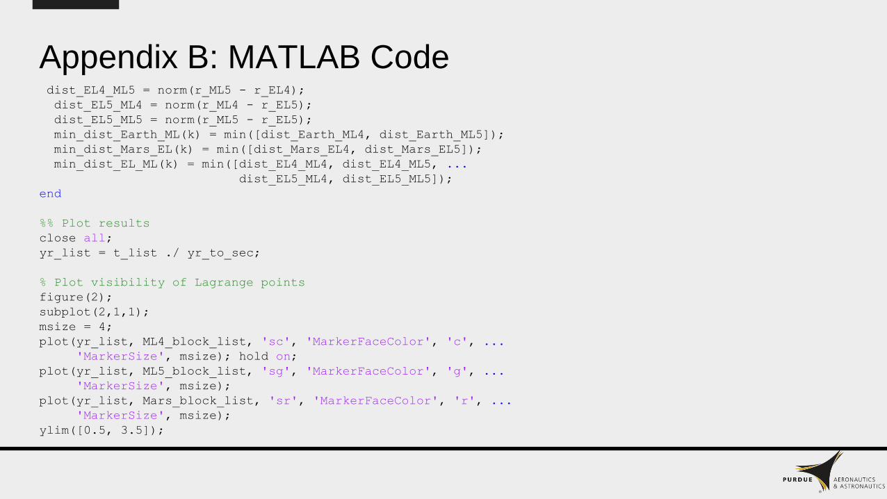
Appendix B: MATLAB Codedist_EL4_ML5 = norm(r_ML5 - r_EL4);

dist_EL5_ML4 = norm(r_ML4 - r_EL5);

dist_EL5_ML5 = norm(r_ML5 - r_EL5);

min_dist_Earth_ML(k) = min([dist_Earth_ML4, dist_Earth_ML5]);

min_dist_Mars_EL(k) = min([dist_Mars_EL4, dist_Mars_EL5]);

min_dist_EL_ML(k) = min([dist_EL4_ML4, dist_EL4_ML5, ...

dist_EL5_ML4, dist_EL5_ML5]);

end

%% Plot results

close all;

yr_list = t_list ./ yr_to_sec;

% Plot visibility of Lagrange points

figure(2);

subplot(2,1,1);

msize = 4;

plot(yr_list, ML4_block_list, 'sc', 'MarkerFaceColor', 'c', ...

'MarkerSize', msize); hold on;

plot(yr_list, ML5_block_list, 'sg', 'MarkerFaceColor', 'g', ...

'MarkerSize', msize);

plot(yr_list, Mars_block_list, 'sr', 'MarkerFaceColor', 'r', ...

'MarkerSize', msize);

ylim([0.5, 3.5]);

Appendix B: MATLAB Codeyticks([1, 2, 3]);

yticklabels({'ML4 Blocked', 'ML5 Blocked', 'Mars Blocked'});

xlabel('time, yrs');

grid on;

title('Visibility of Mars Lagrange Points');

subplot(2,1,2);

plot(yr_list, EL4_block_list, 'sc', 'MarkerFaceColor', 'c', ...

'MarkerSize', msize); hold on;

plot(yr_list, EL5_block_list, 'sg', 'MarkerFaceColor', 'g', ...

'MarkerSize', msize);

plot(yr_list, Mars_block_list, 'sr', 'MarkerFaceColor', 'r', ...

'MarkerSize', msize);

ylim([0.5, 3.5]);

yticks([1, 2, 3]);

yticklabels({'EL4 Blocked', 'EL5 Blocked', 'Mars Blocked'});

xlabel('time, yrs');

grid on;

title('Visibility of Earth Lagrange Points');

%% Compute Lagrange point visibility percentages

percent_ML4 = sum(ML4_block_list == 0)/n_data * 100

percent_ML5 = sum(ML5_block_list == 0)/n_data * 100

percent_ML_both = sum(ML4_block_list == 0 & ML5_block_list == 0)/n_data * 100

Appendix B: MATLAB Codepercent_EL4 = sum(EL4_block_list == 0)/n_data * 100

percent_EL5 = sum(EL5_block_list == 0)/n_data * 100

percent_EL_both = sum(EL4_block_list == 0 & EL5_block_list == 0)/n_data * 100

Appendix B: MATLAB Codefunction [car] = kep2car(kep,GM,atype)

% Name: kep2car.m

% Author: C. Frueh

% Purpose

% To compute the Cartesian position/velocity given Keplerian elements.

% Inputs

% kep - Keplerian elements, (6 x 1) vector with order semi-major axis,

% eccentricity, inclination, right-ascension of the ascending

% node, argument of periapse, mean anomaly

% mu - value of the gravitational parameter of the central body

% atype - units of the angles in the Keplerian elements, 'rad' or 'deg'

% Outputs

% car - Cartesian position/velocity

% Dependencies

% None

sma = kep(1);

ecc = kep(2);

inc = kep(3);

raan = kep(4);

argp = kep(5);

manm = kep(6);

Appendix B: MATLAB Codeif(strcmp(atype,'deg'))

inc = inc*(pi/180.0);

raan = raan*(pi/180.0);

argp = argp*(pi/180.0);

manm = manm*(pi/180.0);

end

itermax = 10;

toler = 1.0D-12;

delta = 1.0;

eanm = manm;

iter = 0;

while((iter < itermax) && (abs(delta) > toler))

iter = iter + 1;

delta = ((eanm - ecc*sin(eanm) - manm)/(1.0 - ecc*cos(eanm)));

eanm = eanm - delta;

end

tanm = 2.0*atan(sqrt((1.0+ecc)/(1.0-ecc))*tan(0.5*eanm));

% if ~isreal(tanm)

% keyboard

% end

r = sma*(1.0-ecc*cos(eanm));

slr = sma*(1.0-ecc*ecc);

angm = sqrt(GM*slr);

Appendix B: MATLAB Codevr = (angm/slr)*ecc*sin(tanm);

vf = (angm/slr)*(1.0+ecc*cos(tanm));

argl = argp + tanm;

cos_s = cos(argl);

sin_s = sin(argl);

cos_i = cos(inc);

sin_i = sin(inc);

cos_W = cos(raan);

sin_W = sin(raan);

R3s = [cos_s,sin_s,0.0;-sin_s,cos_s,0.0;0.0,0.0,1.0];

R1i = [1.0,0.0,0.0;0.0,cos_i,sin_i;0.0,-sin_i,cos_i];

R3W = [cos_W,sin_W,0.0;-sin_W,cos_W,0.0;0.0,0.0,1.0];

T = R3s*R1i*R3W;

x = T(1,1)*r;

y = T(1,2)*r;

z = T(1,3)*r;

xd = T(1,1)*vr + T(2,1)*vf;

yd = T(1,2)*vr + T(2,2)*vf;

zd = T(1,3)*vr + T(2,3)*vf;

car = [x;y;z;xd;yd;zd];

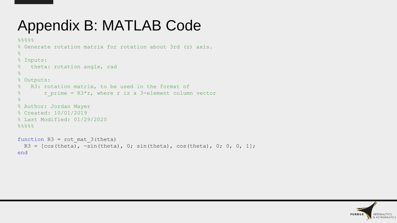
Appendix B: MATLAB Code%%%%%

% Generate rotation matrix for rotation about 3rd (z) axis.

%

% Inputs:

% theta: rotation angle, rad

%

% Outputs:

% R3: rotation matrix, to be used in the format of

% r_prime = R3*r, where r is a 3-element column vector

%

% Author: Jordan Mayer

% Created: 10/01/2019

% Last Modified: 01/29/2020

%%%%%

function R3 = rot_mat_3(theta)

R3 = [cos(theta), -sin(theta), 0; sin(theta), cos(theta), 0; 0, 0, 1];

end

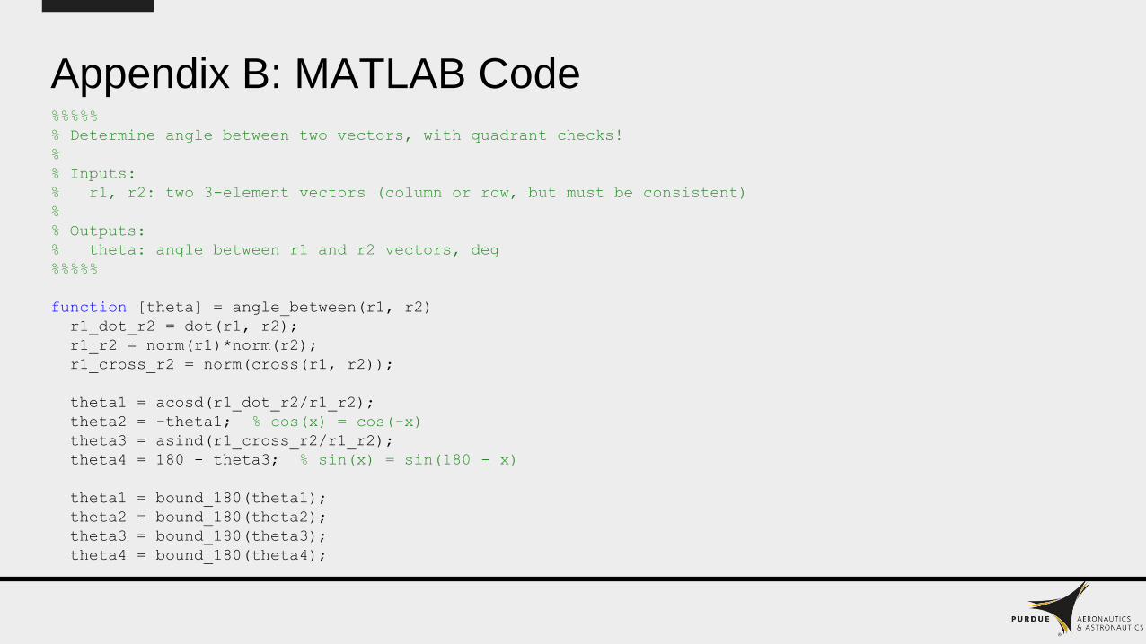
Appendix B: MATLAB Code%%%%%

% Determine angle between two vectors, with quadrant checks!

%

% Inputs:

% r1, r2: two 3-element vectors (column or row, but must be consistent)

%

% Outputs:

% theta: angle between r1 and r2 vectors, deg

%%%%%

function [theta] = angle_between(r1, r2)

r1_dot_r2 = dot(r1, r2);

r1_r2 = norm(r1)*norm(r2);

r1_cross_r2 = norm(cross(r1, r2));

theta1 = acosd(r1_dot_r2/r1_r2);

theta2 = -theta1; % cos(x) = cos(-x)

theta3 = asind(r1_cross_r2/r1_r2);

theta4 = 180 - theta3; % sin(x) = sin(180 - x)

theta1 = bound_180(theta1);

theta2 = bound_180(theta2);

theta3 = bound_180(theta3);

theta4 = bound_180(theta4);

Appendix B: MATLAB Codewiggle = 0.00001;

if abs(theta1 - theta3) < wiggle || abs(theta1 - theta4) < wiggle

theta = theta1;

elseif abs(theta2 - theta3) < wiggle || abs(theta2 - theta4) < wiggle

theta = theta2;

else

fprintf('\ntheta1 = %.4f\n', theta1);

fprintf('theta2 = %.4f\n', theta2);

fprintf('theta3 = %.4f\n', theta3);

fprintf('theta4 = %.4f\n', theta4);

error('no consistent theta');

end

end

Appendix B: MATLAB Code%%%%%

% AAE 450: Spacecraft Design

%

% Determine distances between Earth, Mars, and four possible interplanetary

% relay satellite locations (Sun-Earth L4 and L5, and Sun-Mars L4 and L5).

%

% Author: Jordan Mayer (Mission Design)

% Created: 02/04/2020

% Last Modified: 02/05/2020

%%%%%

%% Preliminary setup

format compact;

addpath('../General Helper Functions/');

AU_to_km = 149597870.700; % Astronomical Units to km

% Set constants and body parameters (from NASA Fact Sheets)

% Gravitational parameters (GM), km^3/s^2

mu_Sun = 132712e6;

mu_Earth = 0.39860e6;

mu_Mars = 0.042828e6;

% Semimajor axes, km

Appendix B: MATLAB Codea_Earth = 149.60e6;

a_Mars = 227.92e6;

% Eccentricities, dimensionless

e_Earth = 0.0167;

e_Mars = 0.0935;

% Mean motions, rad/s

n_Earth = sqrt(mu_Sun/a_Earth^3);

n_Mars = sqrt(mu_Sun/a_Mars^3);

% Longitudes of ascending nodes (J2000), deg

OMEGA_Earth = -11.26064;

OMEGA_Mars = 49.57853;

% Longitudes of perihelion (J2000), deg

omega_bar_Earth = 102.94719;

omega_bar_Mars = 336.04084;

% Arguments of perihelion (J2000), deg

omega_Earth = omega_bar_Earth - OMEGA_Earth;

omega_Mars = omega_bar_Mars - OMEGA_Mars;

% Initial mean anomalies (JD 2459031, 06/30/2020), deg

Appendix B: MATLAB CodeM_0_Earth = 1.771280647464939e2;

M_0_Mars = 3.422533057517022e2;

%% Generate position data

% Set up time steps

yr_to_day = 365;

day_to_hr = 24;

hr_to_sec = 60*60;

yr_to_sec = yr_to_day*day_to_hr*hr_to_sec;

t_f = 15*yr_to_sec;

% simulate for 15 years (from Byrnes, Longuski, and Aldrin: "The inertial

% geometry repeats every 15 years")

n_data = 10000; % number of data points

t_list = linspace(0.0,t_f,n_data).';

% Allocate position arrays, km (only relative coords matter for now)

% (keep it 2-D for now)

r_list_Earth = zeros(n_data, 2); % Earth position

r_list_Mars = zeros(n_data, 2); % Mars position

r_list_ML4 = zeros(n_data, 2); % Mars L4 position

r_list_ML5 = zeros(n_data, 2); % Mars L5 position

r_list_EL4 = zeros(n_data, 2); % Earth L4 position

r_list_EL5 = zeros(n_data, 2); % Earth L5 position

Appendix B: MATLAB Code% Allocate distance arrays, AU

dist_list_Earth_Mars = zeros(n_data, 1);

dist_list_Earth_ML4 = zeros(n_data, 1);

dist_list_Earth_ML5 = zeros(n_data, 1);

dist_list_Mars_EL4 = zeros(n_data, 1);

dist_list_Mars_EL5 = zeros(n_data, 1);

dist_list_EL4_ML4 = zeros(n_data, 1);

dist_list_EL4_ML5 = zeros(n_data, 1);

dist_list_EL5_ML4 = zeros(n_data, 1);

dist_list_EL5_ML5 = zeros(n_data, 1);

% Prepare Keplerian element arrays

% [semimajor axis (km), eccentricity, inclination (deg), longitude of

% ascending node (deg), argument of periapsis (deg), mean anomaly (deg)]

kep_Earth = [a_Earth, e_Earth, 0.0, OMEGA_Earth, omega_Earth, M_0_Earth];

kep_Mars = [a_Mars, e_Mars, 0.0, OMEGA_Mars, omega_Mars, M_0_Mars];

% Get that data!

for k = 1:n_data

delta_t = t_list(k);

% Compute mean anomalies, deg

M_Earth = M_0_Earth + rad2deg(n_Earth*delta_t);

M_Mars = M_0_Mars + rad2deg(n_Mars*delta_t);

Appendix B: MATLAB Code% Update Keplerian element arrays

kep_Earth(6) = M_Earth;

kep_Mars(6) = M_Mars;

% Compute Cartesian vectors [position (km), velocity (km)]

car_Earth = kep2car(kep_Earth, mu_Sun, 'deg');

car_Mars = kep2car(kep_Mars, mu_Sun, 'deg');

if car_Earth(3) > 0 || car_Mars(3) > 0

error('3-D?');

end

% Get 3-D position vectors, km

r_Earth = car_Earth(1:3);

r_Mars = car_Mars(1:3);

r_ML4 = rot_mat_3(deg2rad(60)) * r_Mars;

r_ML5 = rot_mat_3(deg2rad(-60)) * r_Mars;

r_EL4 = rot_mat_3(deg2rad(60)) * r_Earth;

r_EL5 = rot_mat_3(deg2rad(-60)) * r_Earth;

% Store 2-D positions

r_list_Earth(k,:) = r_Earth(1:2);

r_list_Mars(k,:) = r_Mars(1:2);

r_list_ML4(k,:) = r_ML4(1:2);

r_list_ML5(k,:) = r_ML5(1:2);

Appendix B: MATLAB Coder_list_EL4(k,:) = r_EL4(1:2);

r_list_EL5(k,:) = r_EL5(1:2);

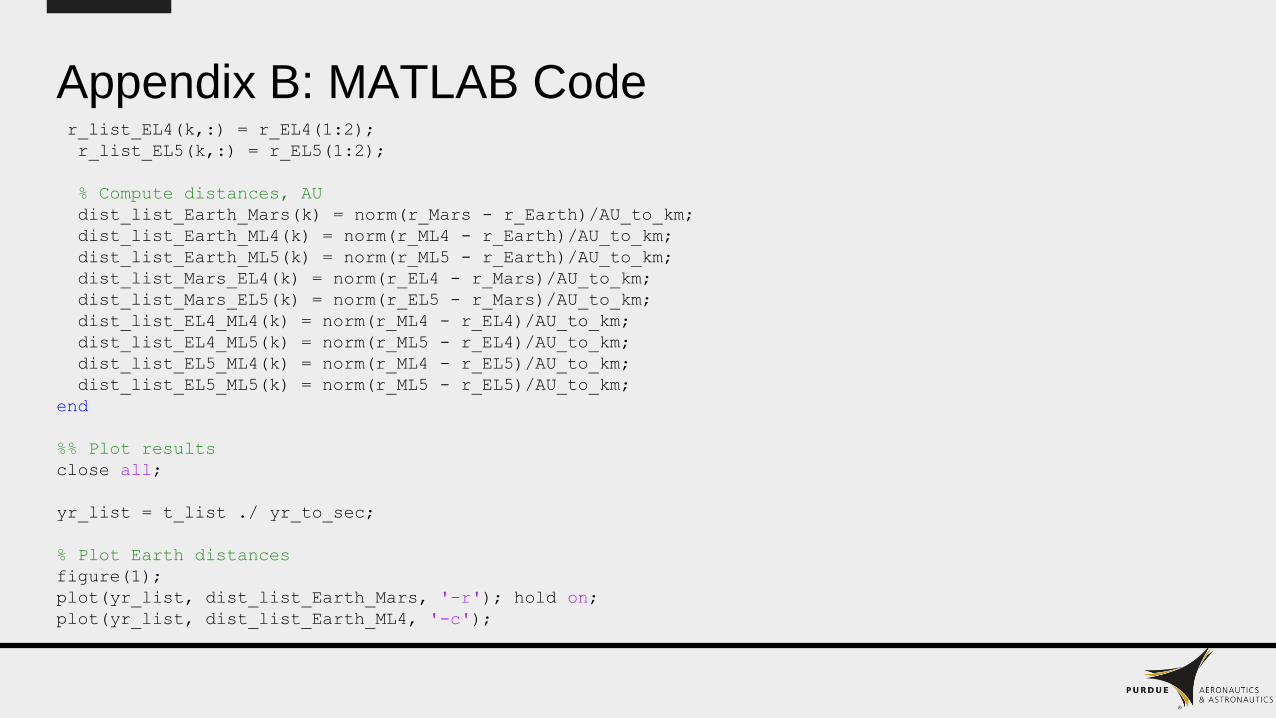
% Compute distances, AU

dist_list_Earth_Mars(k) = norm(r_Mars - r_Earth)/AU_to_km;

dist_list_Earth_ML4(k) = norm(r_ML4 - r_Earth)/AU_to_km;

dist_list_Earth_ML5(k) = norm(r_ML5 - r_Earth)/AU_to_km;

dist_list_Mars_EL4(k) = norm(r_EL4 - r_Mars)/AU_to_km;

dist_list_Mars_EL5(k) = norm(r_EL5 - r_Mars)/AU_to_km;

dist_list_EL4_ML4(k) = norm(r_ML4 - r_EL4)/AU_to_km;

dist_list_EL4_ML5(k) = norm(r_ML5 - r_EL4)/AU_to_km;

dist_list_EL5_ML4(k) = norm(r_ML4 - r_EL5)/AU_to_km;

dist_list_EL5_ML5(k) = norm(r_ML5 - r_EL5)/AU_to_km;

end

%% Plot results

close all;

yr_list = t_list ./ yr_to_sec;

% Plot Earth distances

figure(1);

plot(yr_list, dist_list_Earth_Mars, '-r'); hold on;

plot(yr_list, dist_list_Earth_ML4, '-c');

Appendix B: MATLAB Codeplot(yr_list, dist_list_Earth_ML5, '-m');

title('Distances from Earth'); grid on;

legend('Mars', 'Sun-Mars L4', 'Sun-Mars L5');

xlabel('Time, years'); ylabel('Distance, AU');

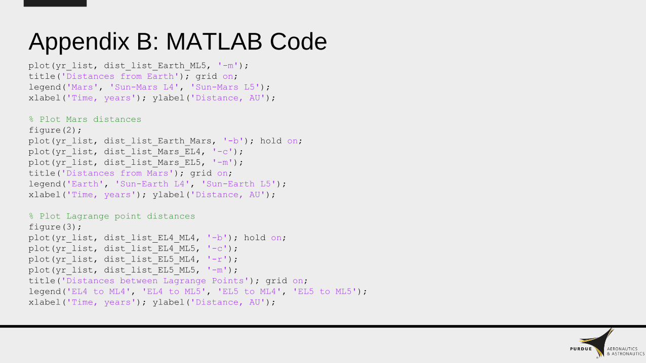
% Plot Mars distances

figure(2);

plot(yr_list, dist_list_Earth_Mars, '-b'); hold on;

plot(yr_list, dist_list_Mars_EL4, '-c');

plot(yr_list, dist_list_Mars_EL5, '-m');

title('Distances from Mars'); grid on;

legend('Earth', 'Sun-Earth L4', 'Sun-Earth L5');

xlabel('Time, years'); ylabel('Distance, AU');

% Plot Lagrange point distances

figure(3);

plot(yr_list, dist_list_EL4_ML4, '-b'); hold on;

plot(yr_list, dist_list_EL4_ML5, '-c');

plot(yr_list, dist_list_EL5_ML4, '-r');

plot(yr_list, dist_list_EL5_ML5, '-m');

title('Distances between Lagrange Points'); grid on;

legend('EL4 to ML4', 'EL4 to ML5', 'EL5 to ML4', 'EL5 to ML5');

xlabel('Time, years'); ylabel('Distance, AU');

Appendix B: MATLAB Code%% Output max distances, AU

% Earth distances

fprintf('\nMax Earth distances:\n\n');

max_dist_Earth_Mars = max(dist_list_Earth_Mars)

max_dist_Earth_ML4 = max(dist_list_Earth_ML4)

max_dist_Earth_ML5 = max(dist_list_Earth_ML5)

min_dist_list_Earth = zeros(n_data,1);

for k=1:n_data

min_dist_list_Earth(k) = min([dist_list_Earth_Mars(k), ...

dist_list_Earth_ML4(k), ...

dist_list_Earth_ML5(k)]);

end

max_dist_Earth_any = max(min_dist_list_Earth)

% Mars distances

fprintf('\nMax Mars distances:\n\n');

max_dist_Mars_EL4 = max(dist_list_Mars_EL4)

max_dist_Mars_EL5 = max(dist_list_Mars_EL5)

min_dist_list_Mars = zeros(n_data,1);

for k=1:n_data

min_dist_list_Mars(k) = min([dist_list_Earth_Mars(k), ...

dist_list_Mars_EL4(k), ...

dist_list_Mars_EL5(k)]);

Appendix B: MATLAB Codeend

max_dist_Mars_any = max(min_dist_list_Mars)

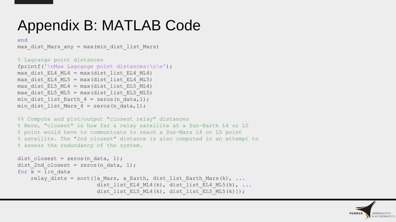
% Lagrange point distances

fprintf('\nMax Lagrange point distances:\n\n');

max_dist_EL4_ML4 = max(dist_list_EL4_ML4)

max_dist_EL4_ML5 = max(dist_list_EL4_ML5)

max_dist_EL5_ML4 = max(dist_list_EL5_ML4)

max_dist_EL5_ML5 = max(dist_list_EL5_ML5)

min_dist_list_Earth_4 = zeros(n_data,1);

min_dist_list_Mars_4 = zeros(n_data,1);

%% Compute and plot/output "closest relay" distances

% Here, "closest" is how far a relay satellite at a Sun-Earth L4 or L5

% point would have to communicate to reach a Sun-Mars L4 or L5 point

% satellite. The "2nd closest" distance is also computed in an attempt to

% assess the redundancy of the system.

dist_closest = zeros(n_data, 1);

dist_2nd_closest = zeros(n_data, 1);

for k = 1:n_data

relay_dists = sort([a_Mars, a_Earth, dist_list_Earth_Mars(k), ...

dist_list_EL4_ML4(k), dist_list_EL4_ML5(k), ...

dist_list_EL5_ML4(k), dist_list_EL5_ML5(k)]);

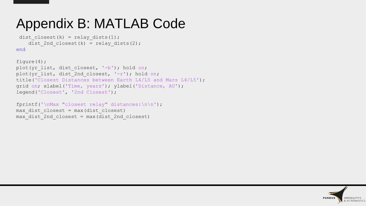
Appendix B: MATLAB Codedist_closest(k) = relay_dists(1);

dist_2nd_closest(k) = relay_dists(2);

end

figure(4);

plot(yr_list, dist_closest, '-b'); hold on;

plot(yr_list, dist_2nd_closest, '-r'); hold on;

title('Closest Distances between Earth L4/L5 and Mars L4/L5');

grid on; xlabel('Time, years'); ylabel('Distance, AU');

legend('Closest', '2nd Closest');

fprintf('\nMax "closest relay" distances:\n\n');

max_dist_closest = max(dist_closest)

max_dist_2nd_closest = max(dist_2nd_closest)

February 20th, 2020

Colin Miller -Backup

Mission Design (Comm Sat)

Orbital Stability Analysis at Earth and Mars

Results

• Used GMAT for all simulations with:

• SRP on - cannon ball model, m = 2 Mg, Area = 42m2

• Gravity model for Earth and Mars were 10x10, and Earth used JGM-2

model, Jaccia-Roberts for drag, and included the Moon as a point mass

• Derivatives (deg/day) were simply the differences in the angular

positions divided by the differences in time

• Model point mass gravities of different relevant bodies via a = Gm/r2 to filter

which bodies were necessary to model

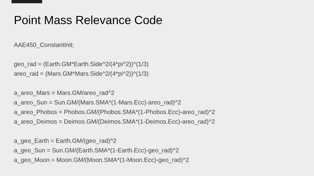
Point Mass Relevance Code

AAE450_ConstantInit;

geo_rad = (Earth.GM*Earth.Side^2/(4*pi^2))^(1/3)

areo_rad = (Mars.GM*Mars.Side^2/(4*pi^2))^(1/3)

a_areo_Mars = Mars.GM/areo_rad^2

a_areo_Sun = Sun.GM/(Mars.SMA*(1-Mars.Ecc)-areo_rad)^2

a_areo_Phobos = Phobos.GM/(Phobos.SMA*(1-Phobos.Ecc)-areo_rad)^2

a_areo_Deimos = Deimos.GM/(Deimos.SMA*(1-Deimos.Ecc)-areo_rad)^2

a_geo_Earth = Earth.GM/(geo_rad)^2

a_geo_Sun = Sun.GM/(Earth.SMA*(1-Earth.Ecc)-geo_rad)^2

a_geo_Moon = Moon.GM/(Moon.SMA*(1-Moon.Ecc)-geo_rad)^2

References

[1] “Earth Fact Sheet.” NASA, NASA,

nssdc.gsfc.nasa.gov/planetary/factsheet/earthfact.html.

[2] “Mars Fact Sheet.” NASA, NASA,

nssdc.gsfc.nasa.gov/planetary/factsheet/marsfact.html.

[3] Silva, Juan J., and Pilar Romero. “Optimal Longitudes Determination for

the Station Keeping of Areostationary Satellites.” Planetary and Space

Science, Pergamon, 17 Feb. 2013,

www.sciencedirect.com/science/article/pii/S0032063313000044#bbib11.

[4] Romero, Pilar, and Jose M. Gambi. “Optimal Control in the East/West

Station-Keeping Manoeuvres for Geostationary Satellites.” Aerospace

Science and Technology, Elsevier Masson, 1 Oct. 2004,

www.sciencedirect.com/science/article/pii/S1270963804000987.

Backup Slides - 1

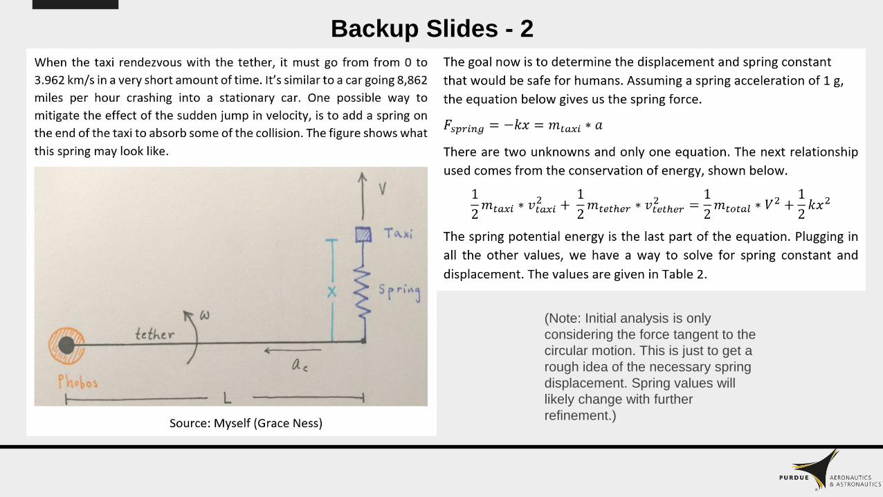
Backup Slides - 2

(Note: Initial analysis is only

considering the force tangent to the

circular motion. This is just to get a

rough idea of the necessary spring

displacement. Spring values will

likely change with further

refinement.)

Backup Slides - 3

Backup Slides - 4

Backup Slides – 5Note: This spin-up time analysis was not presented on, but can be found in the tether folder of the share drive

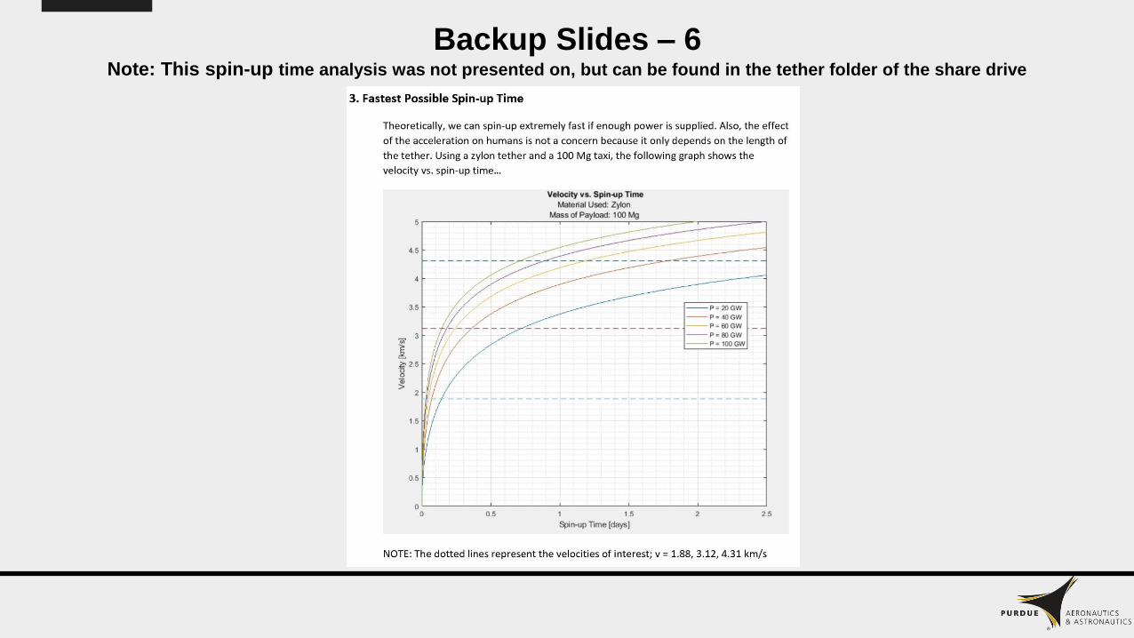
Backup Slides – 6Note: This spin-up time analysis was not presented on, but can be found in the tether folder of the share drive

Backup Slides – 7

MATLAB

February 20, 2020

Dean Lontoc

Backup Slides

Power Source Selection Matrix

Power Source Selection Matrix AnalysisAssumption: Taxi will have power fed to it when it is docked with cycler, tether, or at any launch facility.

Nuclear reactor analysis: Capable of providing continuous power throughout the entire mission, but it has a

massive amount of mass for the energy generated. The SNAP-10A weighed almost 1000kg and only generated

0.5 kW. Repairing it mid-flight could also prove to be a hazard due to radiation hazards. The spent nuclear fuel

is a potential issue in terms of sustainability.

Solar Array: This system is not capable of providing power for every stage of the mission. The solar array must

wait until the taxi vehicle is in space to deploy which would require a battery to power the taxi while it is not

deployed. In addition to that, the solar array would have to be jettisoned before entry into Mars’s atmosphere or

have a mechanism to tuck it away into the taxi. Maintenance on a broken solar array may require a spacewalk

which would be extremely dangerous for the astronauts. If the solar array is jettisoned before atmospheric entry,

creating disposable solar arrays may not be sustainable. It does have the advantage of having less mass and

volume than the other candidates.

Fuel Cell: This power system is in the goldilocks zone of power generation. It can provide continuous power at

every stage of the journey while having reasonable mass and volume. Repairing the fuel cells would be relatively

easy because they would be in the area under the astronauts. It is fully reusable, only requiring reactant resupply at

the end of a leg of the trip.

MATLAB Code

Plugging in mission duration outputs mass and volume

of the power system.

Liquid Oxygen and Hydrogen Storage

Using Power Reactant Storage (PRS)

Storage tanks are to be made of composite materials insulated with 0.25 double aluminized mylar

wrapped in layers over the tank.

10-watt heaters are needed to maintain pressure in tanks, no other power source needed.

PRS systems in the past have successfully spent 21 days in orbit with minimal boil-off.

SourcesA Basic Overview of Fuel Cell Technology Available: https://americanhistory.si.edu/fuelcells/basics.htm.

Aggarwal, V., “Solar Panel Efficiency: What Panels Are Most Efficient?: EnergySage,” Solar News Available:

https://news.energysage.com/what-are-the-most-efficient-solar-panels-on-the-market/.

“An overview of Ball Aerospace cryogen storage and delivery ...” Available:

http://www.ball.com/aerospace/Aerospace/media/Aerospace/Downloads/Aero_tech-comp_cryogen-fuel-

storage.pdf?ext=.pdf.

Chato, D. (2011). NASA Perspectives on Cryo H2 Storage.

“Department of Energy ETEC Closure Project,” ETEC Available:

https://www.etec.energy.gov/Operations/Major_Operations/SNAP_Overview.php.

Dunbar, B., “Fuel Cell Use in the Space Shuttle,” NASA Available:

https://www.nasa.gov/topics/technology/hydrogen/fc_shuttle.html.

“ELECTRICAL POWER SYSTEM,” NASA Available: https://science.ksc.nasa.gov/shuttle/technology/sts-newsref/sts-

eps.html.

“HSF - The Shuttle,” NASA Available: https://spaceflight.nasa.gov/shuttle/reference/shutref/orbiter/eps/pwrplants.html.

“Power,” ESA Available: https://www.esa.int/Science_Exploration/Human_and_Robotic_Exploration/Orion/Power. “Power

Reactant Storage Assembly (PRSA) (Space Shuttle). PRSA hydrogen and oxygen DVT tank

refurbishment,” NASA Available: https://ntrs.nasa.gov/search.jsp?R=19940012449.

January 30, 2020

Jacob Nunez-Kearny - Backup

Power & Thermal

Cycler: Power Generation & Storage

Power system specifications

Data for chosen solar panel, battery and nuclear systems based on TRL rating of

greater than or equal to 4.

Solar Panels Cycler

Power(kW) 1100

Power Area (W/m^2) 300[2]

Specific Power (W/kg) 80[2]

Surface Area (m^2) 8516.112

Mass (kg) 31935.42

Batteries Cycler

Capacity (Amp-hr) 6000

Specific Energy

(Wh/kg) 300[1]

Mass/battery (kg) 20[1]

Total Mass (kg) 2400

RTGs Cycler

Power (kW) 100

Specific Power (W/kg) 7[4]

Total Mass (kg) 14285

Batteries vs nuclear power trade study

For comparison, a battery system was sized for supplying power to keep the

crew alive for 8 months compared to a nuclear radioisotope power system that

provides the same amount of power over the same time.

This study was performed to see if the cycler can house the crew for the longest

journey from Earth to Mars if the main power source was lost. It was also

examined if it would be possible to power the propulsion system with either

batteries or with nuclear power.

Radioisotope generator was chosen as the alternative power source as it is a

constant source of power used in space missions that does not rely upon the

sun.

Trade study dataCycler System Batteries

Power(kW) 1100

Specific Power (Wh/kg) 300[3]

Burn time(sec) 511999.8336

Crew Flight time (sec) 19353600

Energy Required - T (J) 511999833600

Energy Required - HF (J) 1935360000000

Storage Required - T (Wh) 142222176

Storage Required - HF

(Wh) 537600000

Battery Mass - T(kg) 474073.92

Battery Mass - HF(kg) 1792000

Total Battery Mass (kg) 2266073.92

Cycler System RTGs

Power(kW) 100

Specific Power (W/kg) 7[4]

Power Required - T (W) 1000000

Power Required - HF (W) 100000

Nuclear Mass - T(kg) 142857.1429

Battery Mass - HF(kg) 14285.71429

Total Battery Mass (kg) 157142.8571

Cycler

Max Earth to

Earth burn time

(days)

Max Earth to

Mars burn time

(days)

Max Mars to

Earth burn time

(days)

1 2.982706 0 5.925924

2 0 0 3.182045

3 3.582087 4.158183 0

4 1.738419 4.728474 0

Credit to Jennifer Bergeson (MD) for

burn time data.

T is for power

required for

burns. HF is

power required

for life support.

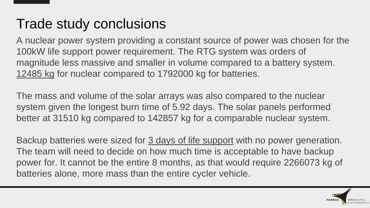
Trade study conclusionsA nuclear power system providing a constant source of power was chosen for the

100kW life support power requirement. The RTG system was orders of

magnitude less massive and smaller in volume compared to a battery system.

12485 kg for nuclear compared to 1792000 kg for batteries.

The mass and volume of the solar arrays was also compared to the nuclear

system given the longest burn time of 5.92 days. The solar panels performed

better at 31510 kg compared to 142857 kg for a comparable nuclear system.

Backup batteries were sized for 3 days of life support with no power generation.

The team will need to decide on how much time is acceptable to have backup

power for. It cannot be the entire 8 months, as that would require 2266073 kg of

batteries alone, more mass than the entire cycler vehicle.

References

[1] Surampudi, S. (2011). Overview of the Space Power Conversion and Energy Storage Technologies.

Jet Propulsion Laboratory, Pasadena.

[2] Beauchamp, P. (2015). Solar Power and Energy Storage for Planetary Missions. Jet Propulsion

Laboratory, Pasadena.

[3] Surampudi, S., et al. (2017). Solar Power Technologies for Future Planetary Science Missions. Jet

Propulsion Laboratory, Pasadena.

[4] Ragheb, M. (2011). RadioIsotopes Power Production. Stanford, CA.

February 20, 2020

Carly Kren – Backup Slides

Propulsion Team

Taxi - Reaction Control Systems (RCS)

Slide: 4 of 25

Derivation of Rocket Equation: Hand calcsSlide: 5 of 25

OMS Configurations NPC1: Hand calcsSlide: 6 of 25

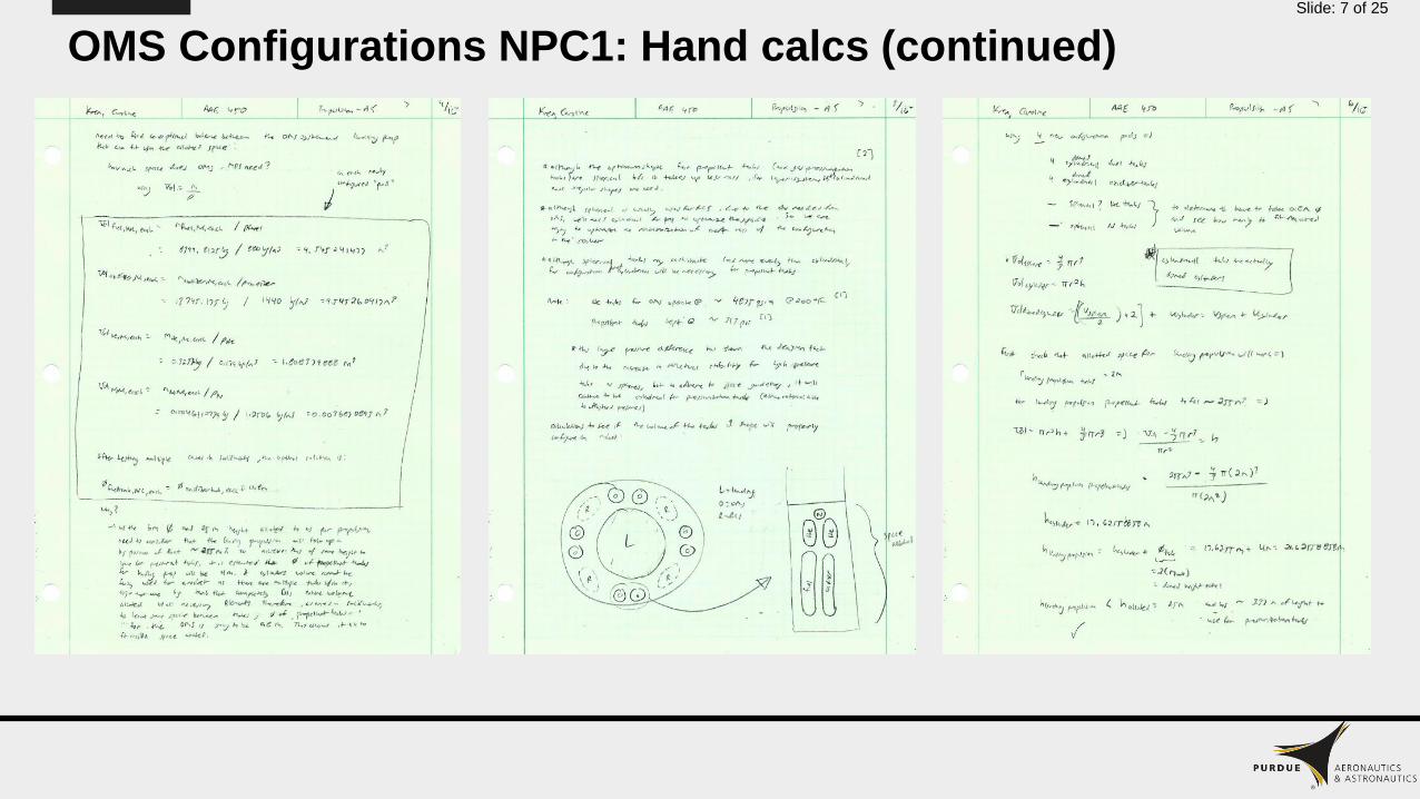
OMS Configurations NPC1: Hand calcs (continued)Slide: 7 of 25

OMS Configurations NPC1: Hand calcs (continued)Slide: 8 of 25

OMS Configurations NPC1: Hand calcs (continued)Slide: 9 of 25

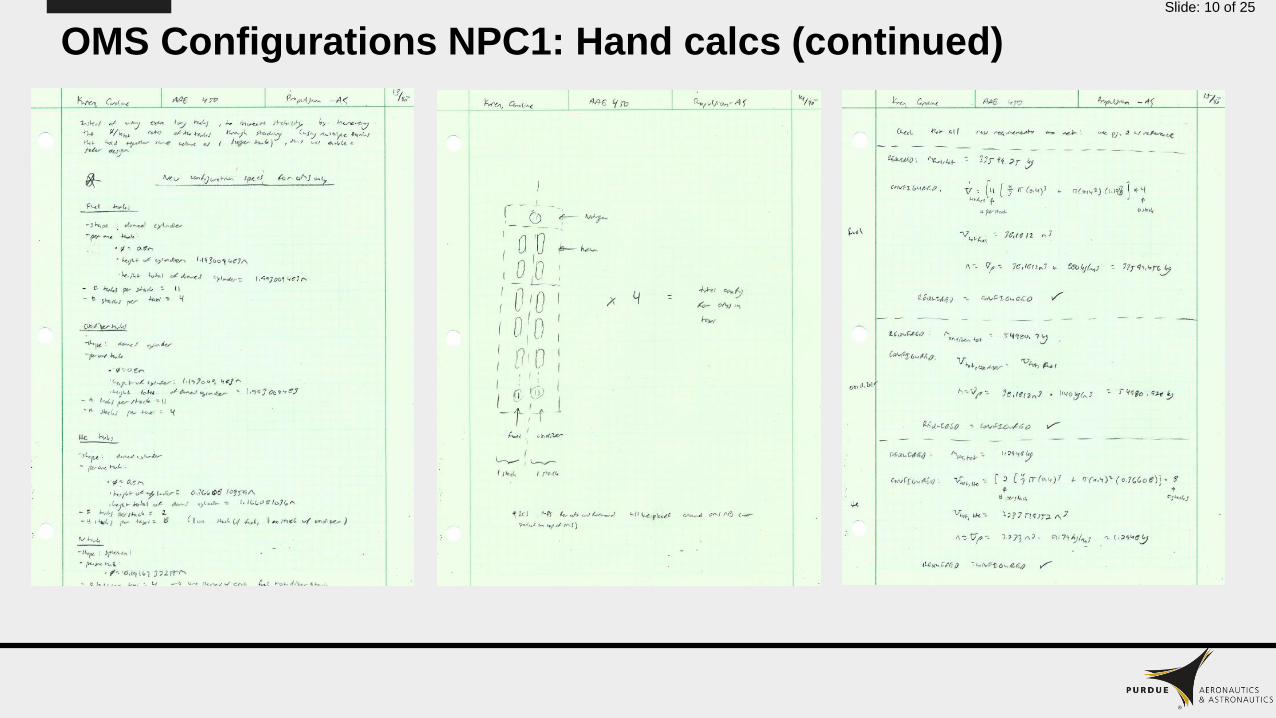
OMS Configurations NPC1: Hand calcs (continued)Slide: 10 of 25

OMS Configurations NPC1: Hand calcs (continued)Slide: 11 of 25

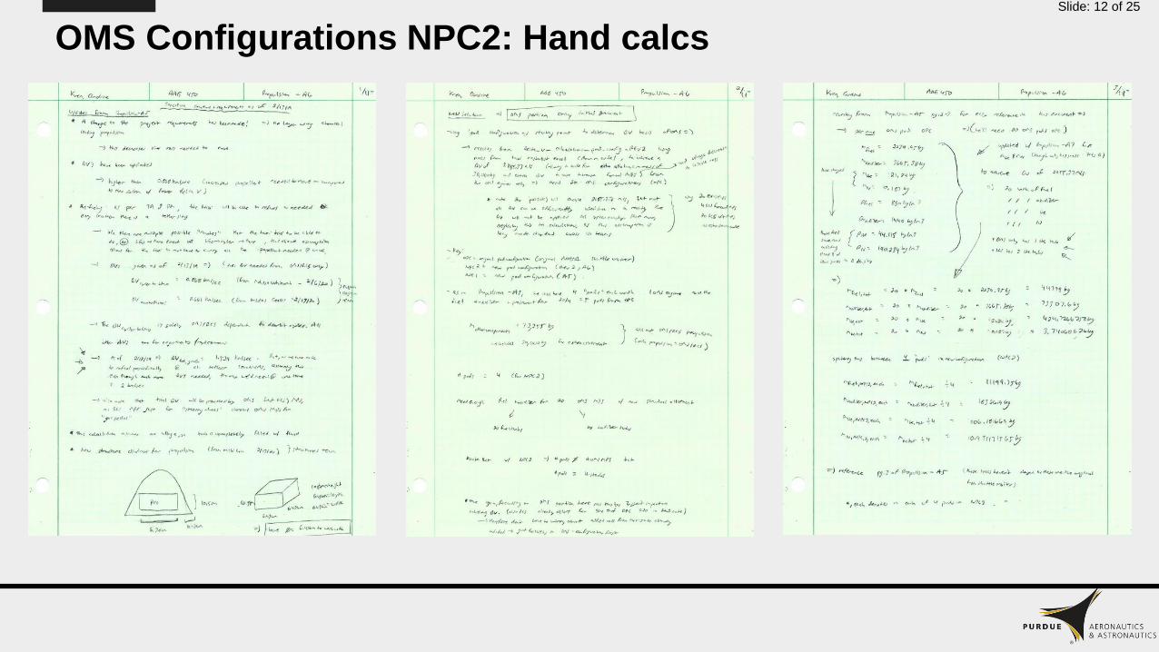
OMS Configurations NPC2: Hand calcsSlide: 12 of 25

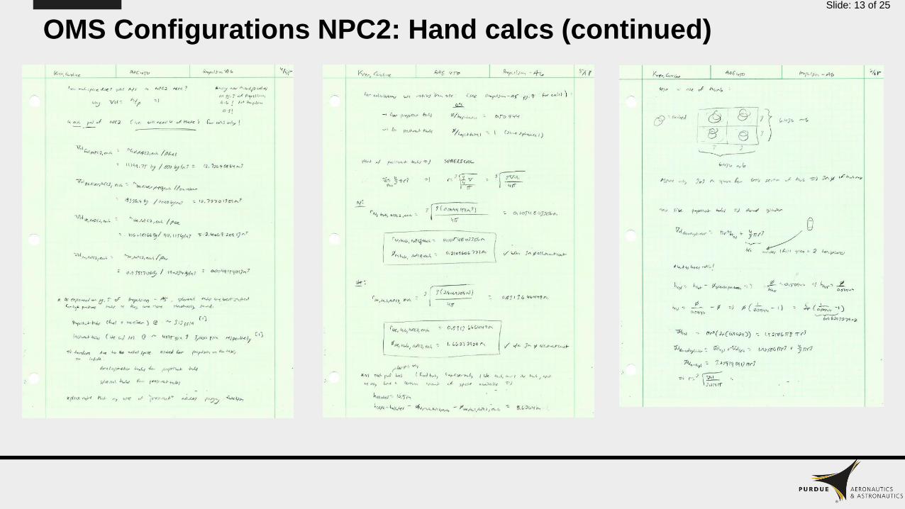
OMS Configurations NPC2: Hand calcs (continued)Slide: 13 of 25

OMS Configurations NPC2: Hand calcs (continued)Slide: 14 of 25

OMS Configurations NPC2: Hand calcs (continued)Slide: 15 of 25

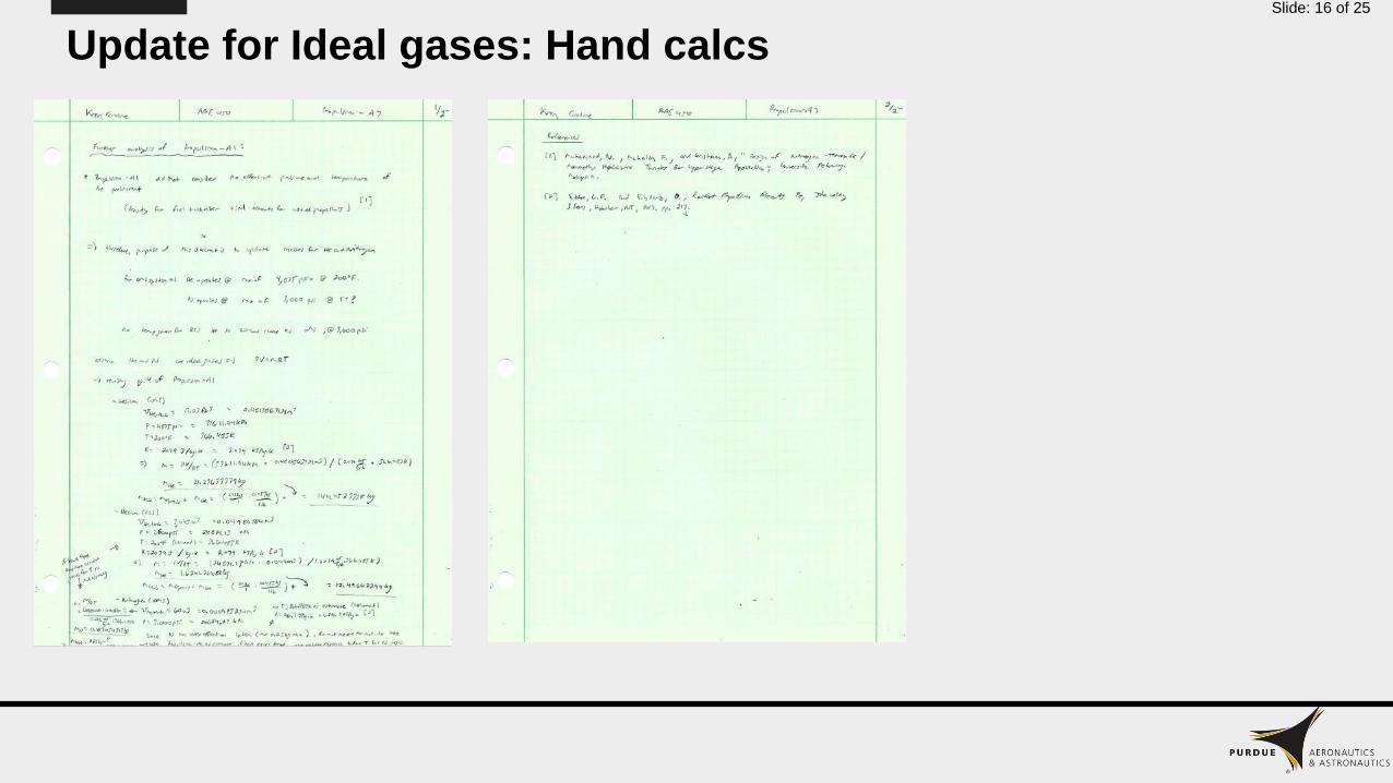
Update for Ideal gases: Hand calcsSlide: 16 of 25

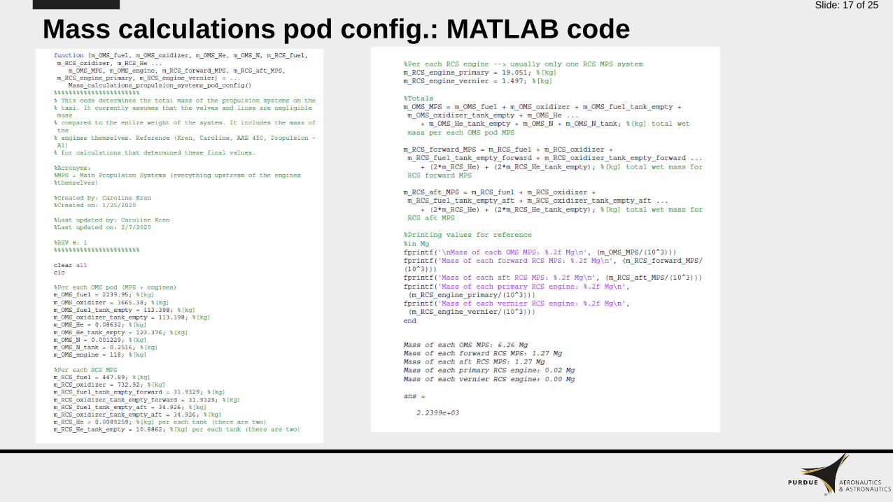
Mass calculations pod config.: MATLAB codeSlide: 17 of 25

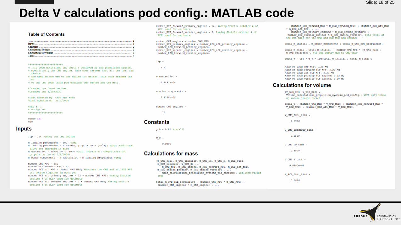
Delta V calculations pod config.: MATLAB codeSlide: 18 of 25

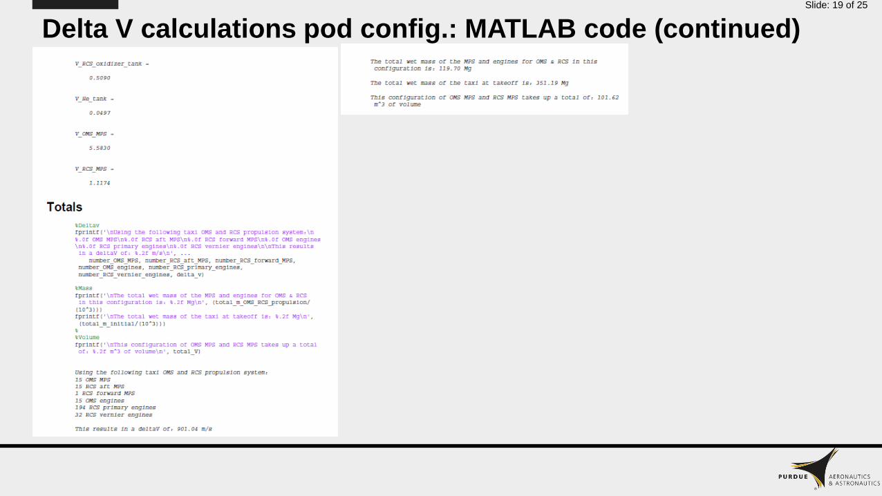
Delta V calculations pod config.: MATLAB code (continued)Slide: 19 of 25

Mass calculations pod config. REV2: MATLAB codeSlide: 20 of 25

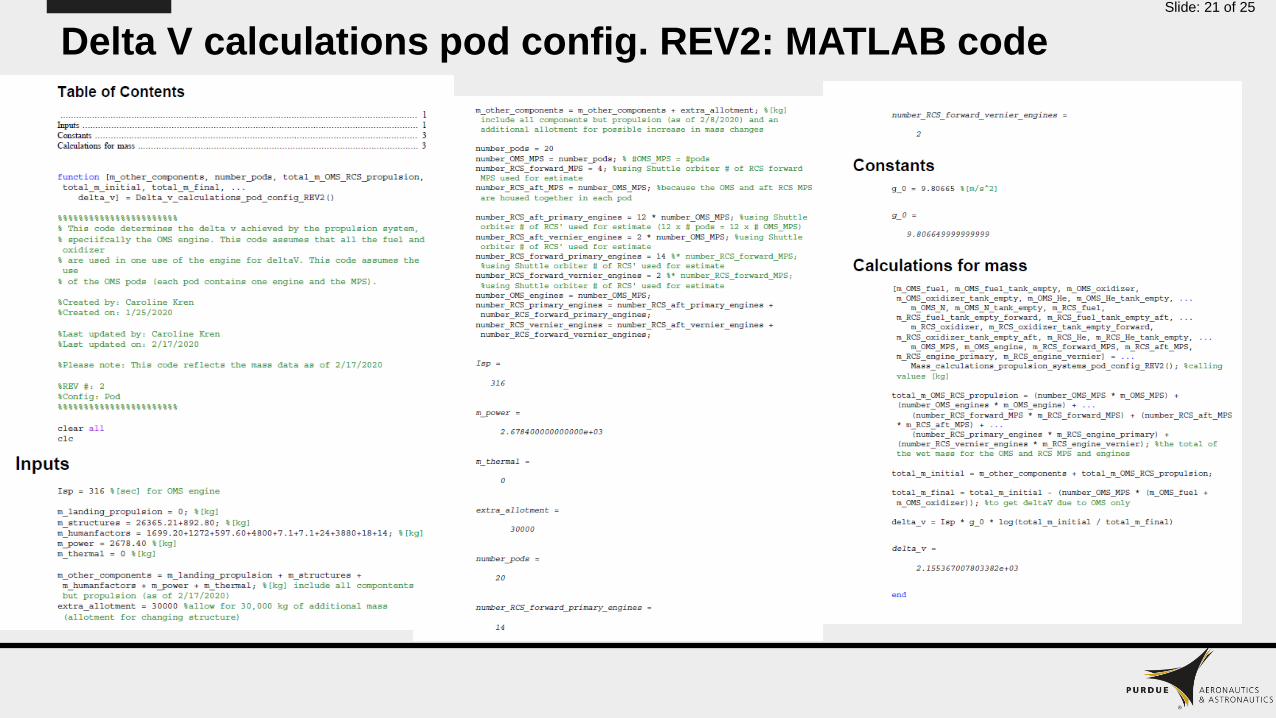
Delta V calculations pod config. REV2: MATLAB codeSlide: 21 of 25

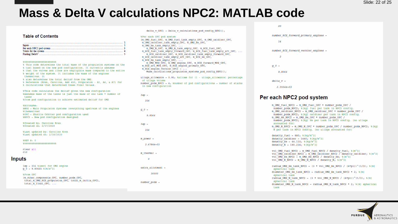
Mass & Delta V calculations NPC2: MATLAB codeSlide: 22 of 25

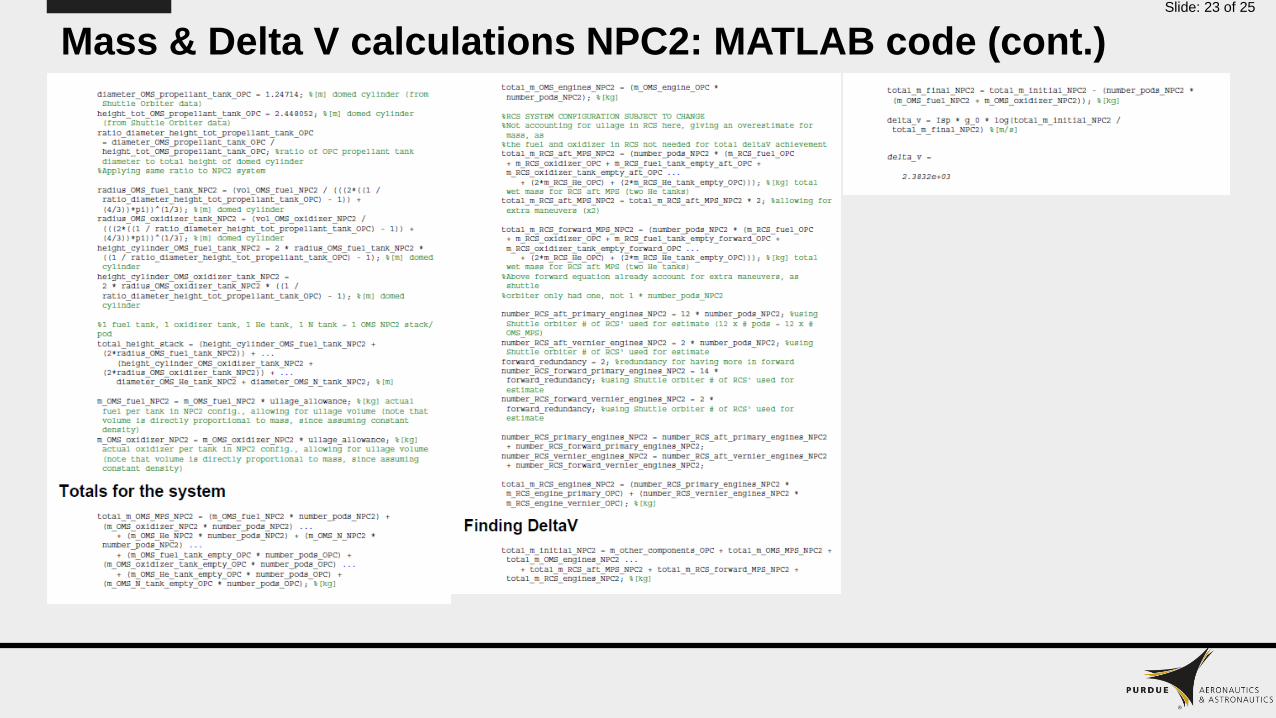
Mass & Delta V calculations NPC2: MATLAB code (cont.)Slide: 23 of 25

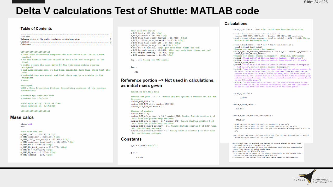
Delta V calculations Test of Shuttle: MATLAB codeSlide: 24 of 25

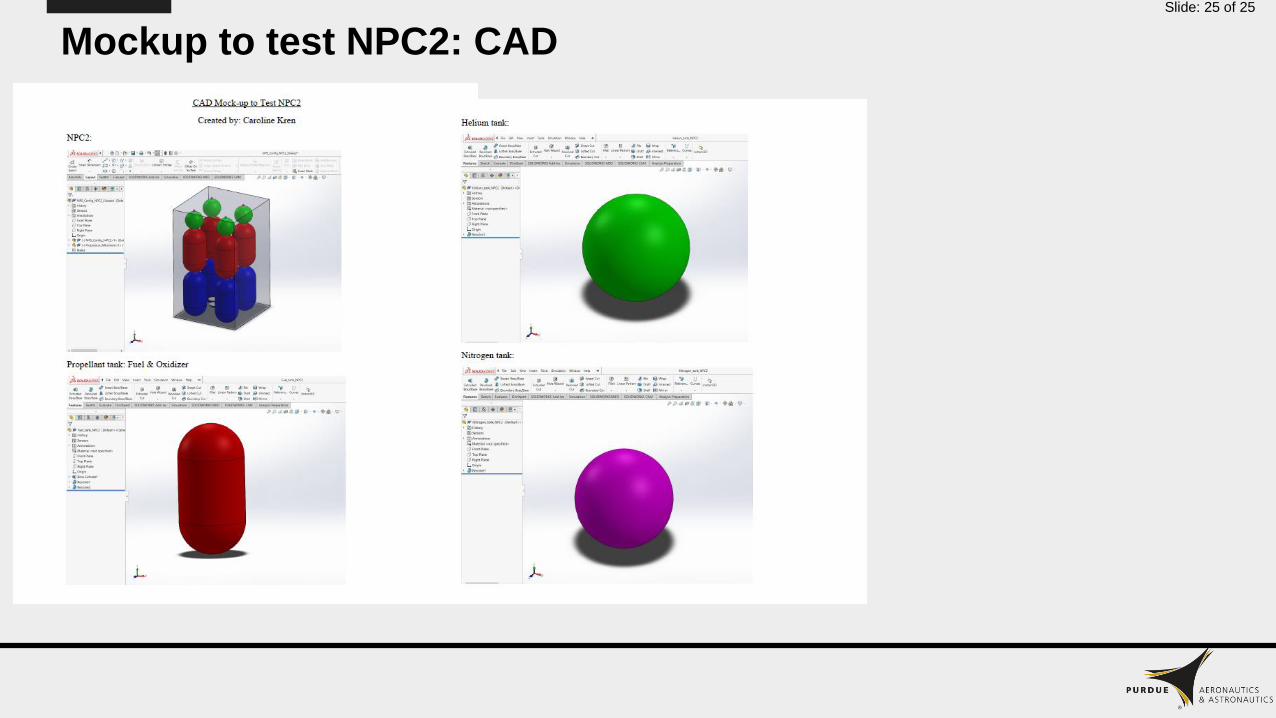
Mockup to test NPC2: CADSlide: 25 of 25

February 20, 2020

Griffin Pfaff – Backup Slides

Propulsion

Cycler - Main Propulsion System

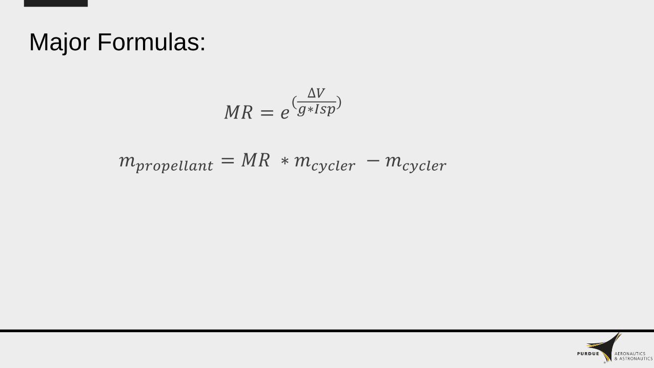
Major Formulas:

𝑀𝑅 = 𝑒(∆𝑉

𝑔∗𝐼𝑠𝑝)

𝑚𝑝𝑟𝑜𝑝𝑒𝑙𝑙𝑎𝑛𝑡 = 𝑀𝑅 ∗ 𝑚𝑐𝑦𝑐𝑙𝑒𝑟 −𝑚𝑐𝑦𝑐𝑙𝑒𝑟

Codecyclermass = 5039; %Mg

taximass = 60; %Mg

totalmass = cyclermass + 3*taximass;

%Mg

forceneed = totalmass * .01; %N

x3mass = .23 %Mg

x3thrust = 5.4; %N

numx3 = 10;

fullthrust = x3thrust * numx3; %N

excessthrust = fullthrust - forceneed

%N

x3power = 100; %kw

fullpower = x3power * numx3 %kw

propflow = 3900; %cm^3/min

isp = 2470;

deltav = 324; %m/s

g = 9.80665; %m/s^2

density = 2.942 %Mg/m^3

mr = exp(deltav/(g*isp));

totalpropmass = mr*totalmass -

totalmass %Mg

totalpropvolume =

totalpropmass/(density) %m^3

systemmass = totalpropmass +

x3mass*numx3 %Mg

isp2 = 450; %liquMid oxygen-liquid

hydrogen

mr2 = exp(deltav/(g*isp2));

totalpropmass2 = mr2*totalmass -

totalmass %Mg

excessthrust =

1.8100

fullpower =

1000

totalpropmass =

70.2785

totalpropvolume =

23.8880

systemmass =

72.5785

totalpropmass2 =

397.5937

Output:

References

[1] Hall, S. J., Jorns, B. A., and Gallimore, A. D., “High-Power

Performance of a 100-kW Class Nested Hall Thruster”, 35th

International Electric Propulsion Conference Georgia Institute

of Technology, Atlanta, GA, 2017.

[2] Lox/LH2 http://www.astronautix.com/l/loxlh2.html [Accessed

19 Feb. 2020]

February 20, 2020

Arch PleumpanyaBackup Slides

Propulsion Team

Mass Driver

Kinematics

- Given escape velocity 𝑉𝑒𝑠𝑐 (5.0 km/s for Mars and 2.5 km/s for Luna)

- Determined acceleration for certain track lengths a =𝑉𝑒𝑠𝑐2

2∆𝑥

- Determined launch duration from ∆𝑡 =𝑉𝑒𝑠𝑐

𝑎

- Given a mass estimate of suspension system required 𝑚𝑠𝑢𝑠𝑝𝑒𝑛𝑠𝑖𝑜𝑛

- Determined force by 𝐹 = 𝑚𝑣𝑒ℎ𝑖𝑐𝑙𝑒 +𝑚𝑠𝑢𝑠𝑝𝑒𝑛𝑠𝑖𝑜𝑛 𝑎

- Determined power by 𝑃 =𝐹∆𝑥

∆𝑡, assuming 50% efficiency

clear

clc

close all

set(0,'DefaultLineLineWidth',1.5);

%

%% Kinematic equations on mass driver

g = 9.81; % Earth's gravitational acceleration [m/s2]

V_esc_mars = 5000; % Mars' escape velocity [m/s]

V_esc_moon = 2500; % Moon's escape velocity [m/s]

x_track_moon = linspace(50000,200000); % possible range of driver

length on the Moon [m]

acc_moon = V_esc_moon^2/2./x_track_moon; % vehicle acceleration on

the Moon [m/s2]

delta_t_moon = V_esc_moon./acc_moon; % launch duration on the Moon

[s]

x_track_mars = linspace(300000,700000); % possible range of driver

length on Mars [m]

acc_mars = V_esc_mars^2/2./x_track_mars; % vehicle acceleration on

Mars [m/s2]

delta_t_mars = V_esc_mars./acc_mars; % launch duration on Mars [s]

%

%% Calculate force required at chose acceleration

m_taxi = 100e3; % estimated vehicle mass [kg]

acc_g_moon = 2; % chosen acceleration limit on the Moon [9.81 m/s2]

F_req_moon = 1.5*m_taxi*acc_g_moon*g; % force required on the Moon

[N]

acc_g_mars = 2; % chosen acceleration limit on Mars [9.81 m/s2]

F_req_mars = 1.5*m_taxi*acc_g_mars*g; % force required on Mars [N]

%

To find the propellant savings, the rocket equation is used:

∆𝑉 = 𝑔0𝐼𝑠𝑝 ln𝑚𝑖𝑛𝑖𝑡𝑖𝑎𝑙

𝑚𝑓𝑖𝑛𝑎𝑙

where propellant mass fraction is 𝜆 =𝑚𝑝𝑟𝑜𝑝𝑒𝑙𝑙𝑎𝑛𝑡

𝑚𝑡𝑜𝑡𝑎𝑙.

Rearranged,

𝑚𝑝𝑟𝑜𝑝𝑒𝑙𝑙𝑎𝑛𝑡 = 𝜆𝑚𝑡𝑎𝑥𝑖

expΔ𝑉𝑔0𝐼𝑠𝑝

− 1

1 − 1 − 𝜆 expΔ𝑉𝑔0𝐼𝑠𝑝

Assuming parameters from the Atlas V where 𝜆 = 0.93 and

𝐼𝑠𝑝 = 338 𝑠.

Calculated using velocities slightly higher than escape

For further technical specification on the maglev system:

- For the propulsion aspect, we are looking at a three-phase,

single-sided, short-primary, linear induction motor.

- For the levitation aspect, we are looking at null-flux coils as

means for electrodynamic suspension.

February 20, 2020

Steven Lach

Structures

Tether Sling, ED Tether, and Mass Drivers

Backup Slides

1

References

3

Taxi Mass: Taxi Masterlist

Aluminum 6061 T6 Properties: ASM Aluminum Data Sheet

http://asm.matweb.com/search/SpecificMaterial.asp?bassnum=

MA6061T6

ΔV: Mission Design Presentations

Tether Calculation Code

3

Concept Development

3

Tether Sling Changes

• 3 Tethers spaced 120 degrees apart.

• Added the gondola system to the requirements which

requires a sheath. This will be in effect on Luna and Mars

• Tethers with sheath will use Zylon fiber instead of Dyneema

fiber due to better tensile strength and mass estimates.

Mass Driver Sled Changes

• The sled will use a Maglev system for propulsion.

• Sled design is heavily dependent on taxi design and mass.

ED Tether

• Electric motor propulsion with electrodynamic orbit

maintenance.

Taxi Connector Design Ideas

3

System that is modeled off of an aircraft carrier arresting wires.

Taxi snags a wire in order to attach to the tether.

Further talks with taxi structures needs to happen in order to

develop the system.

• They have been busy with the taxi redesign

Tether Hub/Torque Arm Design

3

Hub: Large spinning disk to which the torque arms will be

attached to. Material will probably be Aluminum 6061 T6 or

something similar.

Torque Arms: Material will likely be Aluminum 6061 T6. The

cross section design will be analyzed soon.

For tethers with the gondola system, maybe have the torque

arm be hollow and large enough that the people can disembark

the gondola and enter inside the torque arm to make their way

to the central axis of the tether. This would allow them to be

transported down to ground level through the central axis.

This idea is still under consideration and feasibility analysis is

needed.

Mass Driver Sled Design

3

See slide two for diagram of sled. Dimensions are needed

based on the taxi dimensions.

Further Mass Driver structures problems will be passed off to

Erick Smith (CAD) from now on.

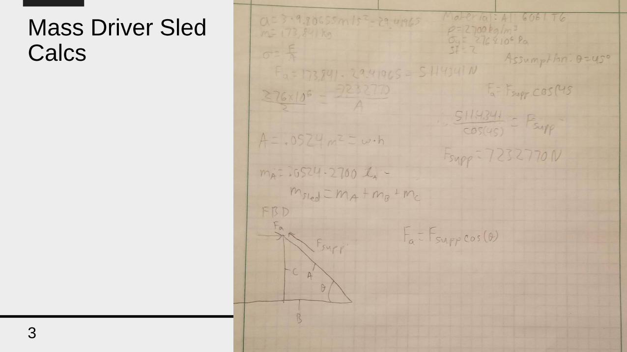
Mass Driver Sled Calcs

3

• Aluminum 7075 – T6 [1]

• Carbon Fiber: HexTow AS4C [3]

Nicki Liu Backup – Material Properties

Mechanical Properties Metric English Comments

Ultimate Tensile Strength >= 572 Mpa >= 83000 psi Wire, rod, bar and shapes

Yield Tensile Strength >= 503 Mpa >= 73000 psi Wire, rod, bar and shapes

Elongation at Break >= 11 % >= 11 % Wire, rod, and bar (rolled or

cold finished)

Modulus of Elasticity 71.7 Gpa 10400 ksi

Fatigue Strength 159 MPa 23000 psi completely reversed stress

Melting Point 477 - 635 °C 890 - 1175 °F

Thermal Conductivity 130 W/m-K 900 BTU-in/hr-ft²-°F

Mechanical Properties Metric English

Bulk Density 1.78 g/cm3 0.0643 lb/in3

Ultimate Tensile Strength 4,654 MPa 675 ksi

Tensile Modulus (Chord 6000-

1000)

231 GPa 33.5 Msi

Weight/Length 0.200 g/m 11.2 x 10-6 lb/in

Approximate Yield 5.00 m/g 7,441 ft/lb

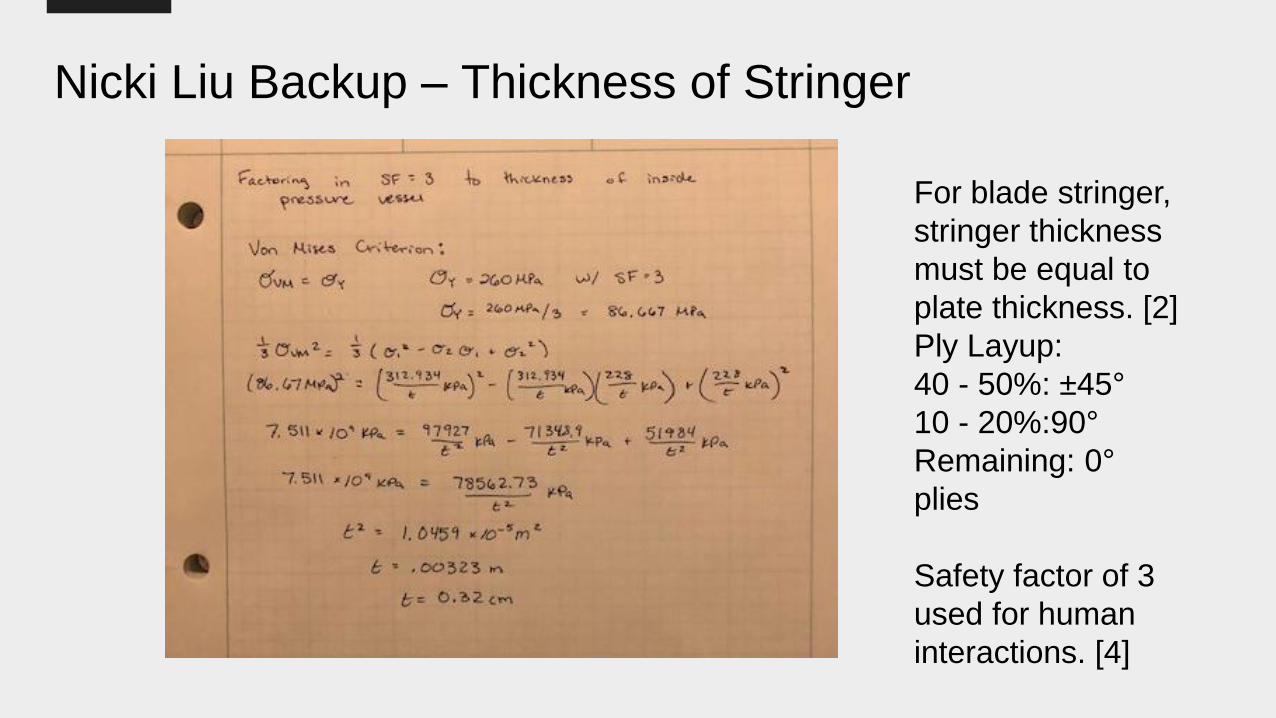
Nicki Liu Backup – Thickness of Stringer

For blade stringer,

stringer thickness

must be equal to

plate thickness. [2]

Ply Layup:

40 - 50%: ±45°

10 - 20%:90°

Remaining: 0°

plies

Safety factor of 3

used for human

interactions. [4]

Nicki Liu Backup – References[1] “Aluminum 7075-T6,” ASM Material Data Sheet Available:

http://asm.matweb.com/search/SpecificMaterial.asp?bassnum=MA7075T6.

[2] Arunkumar, K. N., and Lohith, N., “Effect of Ribs and Stringer Spacings on the Weight of Aircraft

Structure for Aluminum Material,” ARPN Journal of Engineering and Applied Sciences, vol. 12, Jan. 2012,

pp. 1006–1012.

[3] “HexTow® AS4C Carbon Fiber,” Hexcel Available:

https://www.hexcel.com/Resources/DataSheets/Carbon-Fiber.

[4] Japan Aerospace Exploration Agency, “Technical Standard for High Pressure Gas Equipment for Space

Use,” JAXA, vol. JERG-0-001D, Mar. 2016.

[5] Imran, M., Shi, D., Tong, L., and Waqas, H. M., “Design optimization of composite submerged cylindrical

pressure hull using genetic algorithm and finite element analysis,” Ocean Engineering Available:

https://www.sciencedirect.com/science/article/pii/S0029801819305918#bib23.