Section 7 Population Fragmentation Historic Distribution Current Distribution

Section 7Population Fragmentation

HistoricDistribution

CurrentDistribution

When a population is fragmented, differentfragments will have different initial allelefrequencies by chance.

The extent of diversification in allele frequenciescan be measured as variance in allele freq. as:

pp22 = pq/2N = pq/2Nee

Thus, there will be greater variance & largerdifferentiation of allele frequencies among smallfragments.

Additionally, on average, fragmented popualtionshave reduced heterozygosity and increasedvariance in heterozygosity across loci withinpopulations.

The average reduction in heterozygosity due tosampling from the base population is 1/2N1/2Nee.

The initial reduction is minor unless the populationfragments are very small (< 10).

As heterozygosity is lost within fragments &allele frequencies drift among fragments, thereis a deficiency of heterozygotes when comparedto HWE for the entire population and this isknown as the “Wahlund EffectWahlund Effect”.

Sometimes population substructuring is not obvious, and as a result, a sample may consist of a group of heterogeneous subsamples from a population.

For example, subpopulations may be separated by subtle physical or ecological barriers that limit movement between groups.

When these subpopulations are lumped together and if there are differences in allele frequencies among these subpopulations, there will be a deficiency of heterozygotes and an excess of homozygotes which is a Wahlund Effect.

All AA All aaWahlund Effect

With increasing fragmentation, population sizewithin each fragment becomes smaller anddifferentiation among fragments increases.

Inbreeding and inbreeding depression will be morerapid in smaller than larger fragments as willgenetic drift and loss of genetic diversity.

Measuring Population Fragmentation: F-statisticsMeasuring Population Fragmentation: F-statistics

Differentiation among fragments or sub-populationsis directly related to the inbreeding coefficientswithin and among sub-populations or fragments.

Using inbreeding coefficients, Sewall Wrightdescribed the distribution of genetic diversitywithin and among population fragments.

He partitioned inbreeding of individuals (II) in thetotal (TT) populations (FFITIT) into that due to:

Inbreeding of individuals relative to theirsub-population (FFISIS)

Inbreeding due to differentiation amongsub-populations, relative to the total population(FFSTST).

More specifically, FFISIS is the probability that twoalleles in an individual are identical by descent.

This is the inbreeding coefficient (FF) averaged across all individuals from all population fragments.

FFSTST, the fixation index, is the effect of thepopulation sub-division on inbreeding.

FFSTST = probability that two alleles drawn atrandom from a single population fragment (eitherfrom different individuals or the same individual)are identical by descent.

With high rates of gene flow among fragments,this probability is low.

With low rates of gene flow among fragments,populations diverge and become inbred and FFSTST increases.

F-statistics are used to understand factors involved in causing a population to deviate from Hardy-Weinberg expectations.

Deviations from HWE has 2 components:

Deviations due to factors within subpopulationsDeviations due to factors among subpopulations

If the deviations result from excess ofHOMOZYGOTESHOMOZYGOTES, there may be selection, inbreeding,or further population subdivision.

If deviations result from excess of HETEROZYGOTESHETEROZYGOTES, there may be overdominantselection or outbreeding.

Terms & Equations for F-statistics

FF = fixation index and is a measure of how much theobserved heterozygosity deviates from HWE

F = (He - Ho)/He

HHII = observed heterozygosity over ALL subpopulations.

HHII = (Hi)/k where Hi is the observed H ofthe ith supopulation and k = number ofsubpopulations sampled.

HHSS = Average expected heterozygosity withineach subpopulation.

HS = (HIs)/k

Where HIs is the expected H within the ithsubpopulation and is equal to 1 - xi

2 wherexi

2 is the frequency of each allele.

HHTT = Expected heterozygosity within the totalpopulation.

HT = 1 - xi2

where xi2 is the frequency of each allele averaged

over ALL subpopulations.

FFITIT measures the overall deviations from HWEtaking into account factors acting withinsubpopulations and population subdivision.

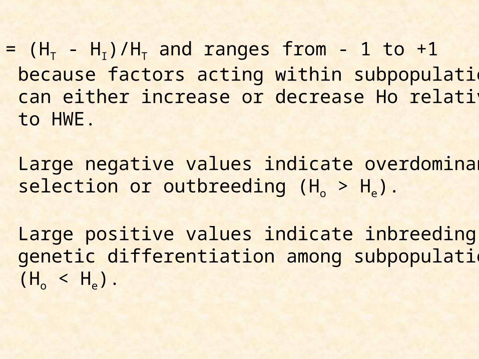
FFITIT = (HT - HI)/HT and ranges from - 1 to +1because factors acting within subpopulationscan either increase or decrease Ho relativeto HWE.

Large negative values indicate overdominanceselection or outbreeding (Ho > He).

Large positive values indicate inbreeding orgenetic differentiation among subpopulations(Ho < He).

FFISIS measures deviations from HWE withinsubpopulations taking into account only thosefactors acting within subpopulations

FFISIS = (HS - HI)/HS and ranges from -1 to +1

Positive FIS values indicate inbreeding ormating occurring among closely related individuals more often than expected underrandom mating.

Individuals will possess a large proportion ofthe same alleles due to common ancestry.

This leads to a reduction in Ho relative to HWE(Ho < He).

Negative FIS suggests outbreeding or matingmating occurring among individuals having differentgenotypes more often than expected underrandom mating (Ho > He).

However, while large negative and positive valuesof FIS indicate non-random mating, the interpretation of FIS is the same as FIT.

Thus, there is the possibility of overdominantselection or further subdivision (Wahlund Effect).

If you knowingly lump different subpopulation into one, FIS will be positive not because ofinbreeding but because of population differentiation.

An understanding of the populations naturalhistory can address the likelihood of thispossibility.

FFSTST measures the degree of differentiation among subpopulations -- possibly due to populationsubdivision.

FST = (HT - HS)/HT and ranges from 0 to 1.

FST estimates this differentiation by comparingHe within subpopulations to He in the totalpopulation.

FST will always be positive because He insubpopulations can never be greater than He inthe total population.

As a general rule of thumb, values of FST that arestatistically different from 0:

0.05 --> 0.15 = moderate genetic differentiation.0.15 --> 0.25 = high genetic differentiation.> 0.25 = very high genetic differentiation.

FST = (FIT - FIS)/(1 - FIS)

Where,

FIS = 1 - (HI/HS)FST = 1 - (HS/HT)FIT = 1 - (HI/HT)

Scenario #1Scenario #1 -- 5 subpopulations, 1 locus, 2 alleles

Given: Observed heterozygosity (HI) = 0.18

PopPop XXii XXjj HHIsIs=1-=1-XXii22

1 0.9 0.1 1-(0.92 + 0.12) = 1 - 0.82 = 0.182 0.9 0.1 1-(0.92 + 0.12) = 1 - 0.82 = 0.183 0.9 0.1 1-(0.92 + 0.12) = 1 - 0.82 = 0.184 0.9 0.1 1-(0.92 + 0.12) = 1 - 0.82 = 0.185 0.9 0.1 1-(0.92 + 0.12) = 1 - 0.82 = 0.18Ave HHS S = = HHIsIs/k = 0.18/k = 0.18Ave 0.9 0.1 HHTT = 1 - = 1 - xxii

22 = 0.18 = 0.18

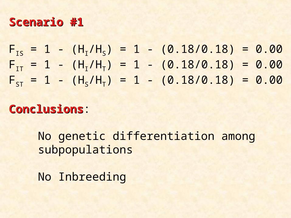
Scenario #1Scenario #1

FIS = 1 - (HI/HS) = 1 - (0.18/0.18) = 0.00FIT = 1 - (HI/HT) = 1 - (0.18/0.18) = 0.00FST = 1 - (HS/HT) = 1 - (0.18/0.18) = 0.00

ConclusionsConclusions:

No genetic differentiation among subpopulations

No Inbreeding





22 = 0.18 = 0.18




No genetic differentiation among subpopulations

Inbreeding!





22 = 0.50 = 0.50




Genetic differentiation among subpopulations

No Inbreeding





22 = 0.50 = 0.50




Genetic differentiation among subpopulations

Inbreeding!

Examples thus far have dealt with a singlehierarchical level.

However, there may be genetic differentiationwithin subpopulations which would create additionalhierarchical levels: localities within subpopulations.

Data can be partitioned into various hierarchicallevels to determine what geographicalfactors most likely explain population differentiation.

HHLiLi = Observed heterozygosity within localities

HHLL = HLi/k

HHIsIs = 1 - xi2 = expected heterozygosity within

subpopulations

HHSS = HIs/k

FFLSLS measures the proportion of the total geneticvariation attributable to divergence amonglocalities within subpopulations.

FFLSLS = (HS - HL)/HT

FFLTLT measures the proportion of the total geneticvariation attributable to localities

FFLTLT = (HT - HL)/HT

FFSTST measures the proportion of the total geneticvariation attributable to subpopulations

FFSTST = (HT - HS)/ HT

Scenario 1Scenario 1subpop loc. xi xj HLi xi xj HSi

1 1 0.8 0.2 0.32 0.8 0.2 0.322 0.8 0.2 0.32

2 3 0.2 0.8 0.324 0.3 0.7 0.42 0.27 0.73 0.39115 0.3 0.7 0.42

0.36 = HL

Ave 0.43 0.52 0.4992 = HT

HS = weighted ave of HSi = [(2X0.32)+(3X0.3911)/5HS = 0.3627

FLS = (HS - HL)/HT

= (0.3627 - 0.36)/0.4992 = 0.005

FLT = (HT - HL)/HT

(0.4992 - 0.36)/0.4992 = 0.279

FST = (HT - HS)/HT

(0.4992 - 0.3627)/0.4992 = 0.273

Scenario 2Scenario 2subpop loc. xi xj HLi xi xj HSi

1 1 0.8 0.2 0.32 0.6 0.4 0.482 0.4 0.6 0.48

2 3 0.7 0.3 0.424 0.3 0.7 0.42 0.47 0.53 0.4985 0.4 0.6 0.48

0.424 = HL

Ave 0.52 0.48 0.4992 = HT

HS = weighted ave of HSi = [(2X0.48)+(3X0.498)/5HS = 0.491

FLS = (HS - HL)/HT

= (0.491 - 0.424)/0.4992 = 0.134

FLT = (HT - HL)/HT

(0.4992 - 0.424)/0.4992 = 0.151

FST = (HT - HS)/HT

(0.4992 - 0.491)/0.4992 = 0.016


In both scenarios, total genetic diversity (HT) is0.4992.

However, in scenario #1, 27.3% of the total geneticdiversity is attributable to differences betweensubpopulations and only 0.5% is due to differencesamong localities within subpopulations.


In scenario #2, 13.4% of the total genetic diversityis attributable to differences between the twosubpopulation and 1.7% is attributable todifferences among localities.

Mortamer Snide graduated with a Ph.D. in wildlife management from Texas A&M University in the early 1900s. Hisdissertation dealt with the distribution and deer of an unknown and unnamed mountain range in Idaho. Because of the ruggedterrain and remoteness of the area, Mortamer spent 15 years collecting observational data on deer in this area to develop amanagement plan. Upon graduating and publishing his dissertation, Mortamer Snide was hired by the Idaho Department of Wildlife Resources to develop a management plan for deer in this area. Because he spent so much time in these mountains, the mountain range was officially named the Mortamer Snide Mountains and the newly developed management area wasnamed the Mortamer Snide Management Area. Based on his work, Mortamer concluded that there were two herds ofdeer on the management area, separated from each other by the Snide Mountain Range. Additionally, his demographicwork suggested that although there appeared to be subdivision within these two regions, there were high levels ofmovement of individuals within each regions such that each regions should be treated as a management unit. Therefore,his management plan was to treat all deer east of the Snide Mountains as one management unit and all deer west of theSnide Mountains as a second management unit.

In recent years, the deer on the Mortamer Snide Management Area have not been doing well. You are enrolled in thePh.D. program at Oklahoma State University and have become very interested in the problem with the deer at theMortamer Snide Management Area. For your dissertation, you spent several years performing demographic studies ofthe deer on each side of the Snide Mountain Range. Your observational data indicate that there may actually be twoheards within each region. However, to test this, you collect blood samples from several deer from five groups ofdeer, two on the west side of the Snide Mountains and three from the east side of the Snide Mountains and perform amicrosatellite analysis. The following is a figure illustrating your interpretation of the demographics of the deer populations on the Mortamer Snide Management Area.

Completely Analyze these data

A-2A-2

A-1A-1 B-1B-1

B-2B-2

B-3B-3

Snide Mountains

SubpopulationsLocalities

Snide River

Locus 1 Locus 2AA Aa aa BB Bb bb

A-1 26 27 16 14 19 36A-2 10 18 28 38 6 12B-1 20 23 26 29 14 26B-2 12 8 36 12 6 38B-3 19 25 25 30 20 19

Calculate Observed Heterozygosity (Ho) & Testeach locus in each population for deviations from H.W.E.

Sample A1, Locus 1Ho = 27/69 = 0.3913A = p = (26+26+27)/138 = 0.5725; q = 1 - 0.5725 = 0.4275

OBSOBS EXPEXP (O-E)(O-E)22/E/E26 (0.5725)2X69 = 22.62 0.50527 2X0.5725X0.4275X69 = 33.77 1.35716 (0.4275)2X69 = 12.61 0.911

2 = 2.773

Degrees of Freedom = 3 - 1 - 1 = 1Tabled 2 at = 0.05 and 1 d.f. = 3.84

Sample A1, Locus 2Ho = 19/69 = 0.275B = p = (14+14+19)/138 = 0.3406; q = 1 - 0.3406 = 0.6594


2 = 10.339

Ho = (0.3913 + 0.275)/2 = 0.3332

Sample A2, Locus 1Ho = 18/56 = 0.321A = p = (10+10+18)/112 = 0.3393; q = 1 - 0.3393 = 0.6607


2 = 4.46

Sample A2, Locus 2Ho = 6/56 = 0.107B = p = (38+38+6)/112 = 0.7321; q = 1 - 0.7321 = 0.2679


2 = 29.59

Ho = (0.321 + 0.107)/2 = 0.214

Sample B1, Locus 1Ho = 23/69 = 0.333A = p = (20+20+23)/138 = 0.4565; q = 1 - 0.4565 = 0.5435


2 = 9.34

Sample B1, Locus 2Ho = 14/69 = 0.203B = p = (29+29+14)/138 = 0.5217; q = 1 - 0.5217 = 0.4783


2 = 24.3

Ho = (0.333 + 0.203)/2 = 0.268



2 = 23.67



2 = 29.59

Ho = (0.143 + 0.107)/2 = 0.125



2 = 5.03



2 = 11.29

Ho = (0.362 + 0.290)/2 = 0.326

Calculate HCalculate Hee = 2N(1 - = 2N(1 - ppii22)/(2N - 1))/(2N - 1)

A-1 locus 1: 138[1-(0.3278+0.1828)]/137=0.4930A-1 locus 2 138[1-(0.1160+0.4348)]/137=0.4525He = (0.4930 + 0.4525)/2 = 0.473

A-2 locus 1: 112[1 - 0.5516]/111 = 0.4524A-2 locus 2: 112[1 - 0.6077]/111 = 0.3958He = (0.4524 + 0.3958)/2 = 0.4241

B-1 locus 1: 138[1 - 0.5038]/137 = 0.4998B-1 locus 2: 138[1 - 0.5009]/137 = 0.5027He = (0.4998 + 0.5027)/2 = 0.5013

B-2 locus 1: 112[1 - 0.5918]/111 = 0.4119B-2 locus 2: 112[1 - 0.6078]/111 = 0.3856He = (0.4119 + 0.3856)/2 = 0.3988

B-3 locus 1: 138[1 - 0.5038]/137 = 0.4998B-3 locus 2: 138[1 - 0.5114]/137 = 0.4922He = (0.4998 + 0.4922)/2 = 0.4960

Table of Descriptive Statistics

Locus 1 Locus2Ho He HWE Ho He HWE Ho He

A1 0.391 0.493 Y 0.275 0.453 N 0.333 0.473A2 0.321 0.452 N 0.107 0.396 N 0.214 0.424B1 0.333 0.500 N 0.203 0.502 N 0.268 0.501B2 0.143 0.412 N 0.107 0.386 N 0.125 0.399B3 0.362 0.500 N 0.290 0.492 N 0.326 0.496

Locus 1Locus 1subpop loc. xi xj HLi xi xj HSi

A 1 0.573 0.427 0.489 0.456 0.544 0.4962 0.339 0.661 0.448

B 1 0.457 0.543 0.4962 0.268 0.732 0.392 0.394 0.606 0.4783 0.457 0.543 0.496

0.457 = HL

Ave 0.419 0.581 0.487 = HT

HS = weighted ave of HSi = [(2X0.496)+(3X0.478)]/5HS = 0.485

FLS = (HS - HL)/HT

= (0.485 - 0.457)/0.487 = 0.057

FLT = (HT - HL)/HT

= (0.487 - 0.457)/0.487 = 0.062

FST = (HT - HS)/(HT)

= (0.487 - 0.485)/0.487 = 0.004

Locus 2Locus 2subpop loc. xi xj HLi xi xj HSi

A 1 0.341 0.659 0.449 0.537 0.463 0.4972 0.732 0.268 0.392

B 1 0.522 0.478 0.4992 0.268 0.732 0.392 0.455 0.545 0.4963 0.576 0.424 0.488

0.444 = HL

Ave 0.422 0.578 0.500 = HT

HS = weighted ave of HSi = [(2X0.497)+(3X0.496)]/5HS = 0.496

FLS = (HS - HL)/HT

= (0.496 - 0.444)/0.500 = 0.104

FLT = (HT - HL)/HT

= (0.500 - 0.444)/0.500 = 0.112

FLS = (HT - HS)/(HT)

= (0.500 - 0.496)/0.500 = 0.008

FLS FLT FST

Locus 1 0.057 0.062 0.004

Locus 2 0.104 0.112 0.008

Ave. 0.081 0.087 0.006

F-statistics Locus 1F-statistics Locus 1HI = (0.391+0.321+0.333+0.143+0.362)/5 = 0.399


A1 0.5725 0.4275 0.4894A2 0.3393 0.6607 0.4484B1 0.4565 0.5435 0.4962B2 0.2857 0.7143 0.4082B3 0.4565 0.5435 0.4962Ave HHS S = = HHIsIs/k = 0.4677/k = 0.4677Ave 0.4221 0.5779 HHTT = 1 - = 1 - xxii

22 = 0.4879 = 0.4879

HI = 0.399HS = 0.468HT = 0.488

FIS = 1 - (HI/HS) = 1 - (0.399/0.468) = 0.147

FIT = 1 - (HI/HT) = 1 - (0.399/0.488) = 0.182

FST = 1 - (HS/HT) = 1 - (0.468/0.488) = 0.041

F-statistics Locus 2F-statistics Locus 2HI = (0.275+0.107+0.203+0.107+0.290)/5 = 0.196


A1 0.3406 0.6594 0.4492A2 0.7321 0.2679 0.3923B1 0.5217 0.4783 0.4991B2 0.2678 0.7322 0.3922B3 0.5755 0.4245 0.4886Ave HHS S = = HHIsIs/k = 0.4443/k = 0.4443Ave 0.4875 0.5125 HHTT = 1 - = 1 - xxii

22 = 0.4997 = 0.4997

HI = 0.196HS = 0.4443HT = 0.4997

FIS = 1 - (HI/HS) = 1 - (0.196/0.444) = 0.559

FIT = 1 - (HI/HT) = 1 - (0.196/0.500) = 0.608

FST = 1 - (HS/HT) = 1 - (0.444/0.500) = 0.112

FIS FIT FST

Locus 1 0.147 0.182 0.041Locus 2 0.559 0.608 0.112Ave 0.353 0.395 0.077

Calculation of Pairwise FCalculation of Pairwise FSTST --Locus 1; Population A1 vs. A2

Subpop xi xj HSi

A1 0.5725 0.4275 0.4894A2 0.3393 0.6607 0.4484

HS = 0.4689Ave. 0.4559 0.5441 HT = 0.4961

FST = 1 - (HS/HT) = 1 - (0.4689/0.4961) = 0.055

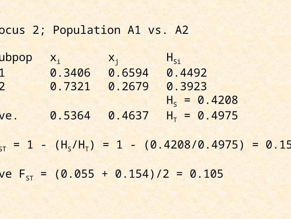
Locus 2; Population A1 vs. A2

Subpop xi xj HSi

A1 0.3406 0.6594 0.4492A2 0.7321 0.2679 0.3923

HS = 0.4208Ave. 0.5364 0.4637 HT = 0.4975

FST = 1 - (HS/HT) = 1 - (0.4208/0.4975) = 0.154

Ave FST = (0.055 + 0.154)/2 = 0.105

Continue this for ALL pairwise comparisons

A1 A2 B1 B2 B3A1 -----A2 0.105 -----B1 0.024 0.031 -----B2 0.046 0.110 0.048 -----B3 0.035 0.021 0.001 0.061 ---

Unweighted Pair-Group Method Using ArithmetricAverages (UPGMA) Clustering Method.

UPGMA computes the average similarity ordissimilarity of a candidate OTU to an extantcluster, weighting each OTU in that clusterequally, regardless of its structural subdivision.

Pairwise FST

A1 A2 B1 B2 B3A1 -----A2 0.105 -----B1 0.024 0.031 -----B2 0.046 0.110 0.048 -----B3 0.035 0.021 0.0010.001 0.061 ---

Step 1Step 1 -- Find the pair(s) of OTUs with the lowestvalue.

Step 2Step 2 -- Recalculate distances with [B1,B3] as anOUT. Differences between OTUs that did not join any cluster are transcribed unchanged fromthe original matrix.

Therefore:[B1,B3] vs. A1 = 1/2(B1A1 + B3A1)

= 1/2(0.024 + 0.035) = 0.030[B1,B3] vs. B2 = 1/2(0.031 + 0.021) = 0.026[B1,B3] vs. B2 = 1/2(0.048 + 0.061) = 0.055

Now:

[B1,B3] A1 A2 B2[B1,B3] -----A1 0.30 -----A2 0.0260.026 0.105 -----B2 0.055 0.046 0.110 -----

Find the smallest difference and repeat the abovesteps until all OTUs cluster!

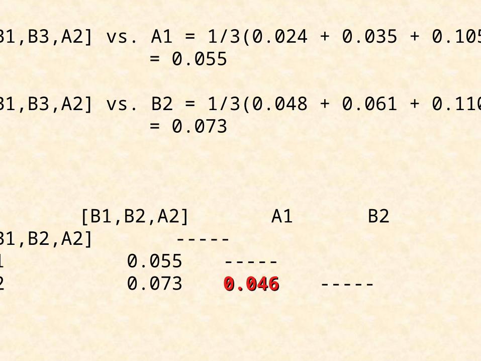
[B1,B3,A2] vs. A1 = 1/3(0.024 + 0.035 + 0.105) = 0.055

[B1,B3,A2] vs. B2 = 1/3(0.048 + 0.061 + 0.110) = 0.073

[B1,B2,A2] A1 B2[B1,B2,A2] -----A1 0.055 -----B2 0.073 0.0460.046 -----

[B1,B3,A2] vs. [A1,B2] =

1/6(0.105 + 0.024 + 0.035 + 0.048 + 0.110 + 0.061)

= 0.064

Final Step is to draw an unrooted dendrogram

SummarySummary:1. B1 clusters with B3 @ 0.0012. A2 clusters with [B1,B3] @ 0.0263. A1 clusters with B2 @ 0.0464. [B1,B3,A2] clusters with [A1,B2] at 0.064

B1 B3 A2 A1 B200.010.020.030.040.050.06

A-2A-2

A-1A-1 B-1B-1

B-2B-2

B-3B-3

Snide Mountains

SubpopulationsLocalities

Snide River

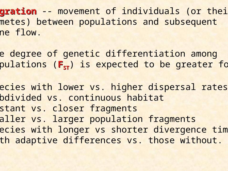
MigrationMigration -- movement of individuals (or theirgametes) between populations and subsequentgene flow.

The degree of genetic differentiation among populations (FFSTST) is expected to be greater for:

species with lower vs. higher dispersal ratessubdivided vs. continuous habitatdistant vs. closer fragmentssmaller vs. larger population fragmentsspecies with longer vs shorter divergence timeswith adaptive differences vs. those without.

Mainland-Island Model of MigrationMainland-Island Model of Migration:

One-Way

Migrationqm qt

m = migration coefficient; proportion of individualson the island that just came from the mainland.

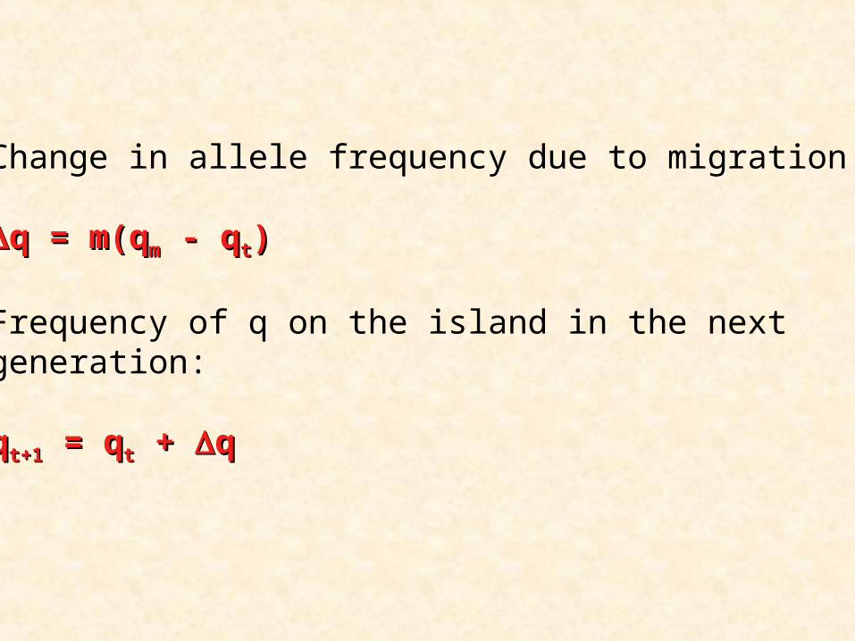
Change in allele frequency due to migration:

q = m(qq = m(qmm - q - qtt))

Frequency of q on the island in the nextgeneration:

qqt+1t+1 = q = qtt + + qq

The Mainland-Island model of gene flow isrealistic for:

the Galapagos Islands & west coast of S. A.

“habitat islands” such as fragmented rainforestsof mountain tops separated by desert.

Island ModelIsland Model:

m is the proportion ofindividuals on any oneisland that came fromelsewhere.

The islands differ in allele frequency, and theaverage allele frequency among all islands is the mean p.

From the point of view of a single island, all otherislands are equivalent of a “mainland”.

Therefore, if q is the allele frequency on agiven island, the recursion equation for the allelefrequency on the island is:

qqt+1t+1 = (m X q) + (1 - m)(q = (m X q) + (1 - m)(qtt))

This is the same equation as the mainland-islandmodel.

The allele frequency on each island will approachthe mean allele frequency across all islands.

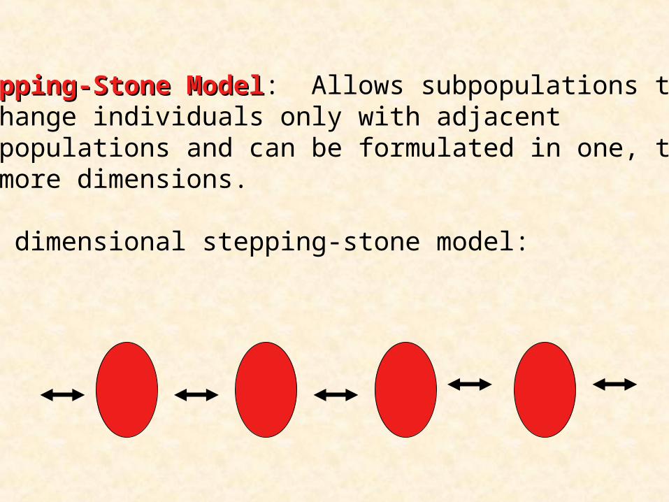
Stepping-Stone ModelStepping-Stone Model: Allows subpopulations toexchange individuals only with adjacent subpopulations and can be formulated in one, two,or more dimensions.

One dimensional stepping-stone model:

Two-Dimensional Stepping-Stone Model:

Migration tends to homogenize populations andthe rate of homogenization depends upon themigration rate, population structure, and difference in allele frequencies.

All subpopulations eventually approach the meanallele frequency of the total population!

Populations diverge from each other as a functionof genetic drift, migration, and local selection.

Drift can have a particularly strong effect onsmall populations and is an inverse function of Ne.

FFSTST = 4N = 4Neem + 1m + 111

If Ne is small, populations will tend to diverge as aresult of random genetic drift and high rates ofmigration (m) are needed to prevent divergence.

Allendorf (1983) has shown that if Nem is > 1, local populations will not tend to divergesignificantly in terms of alleles present.

For example, a pair of populations with a mean Ne

of 1,000 and m = 0.01 would not significantlydiverge by chance alone since Nem = 10.

However, a pair of smaller population, with a meanNe of 100 and the same rate of gene flow(m = 0.01), random drift would be greater and ahigher rate of gene flow would be needed to prevent divergence.

Some populations and species in nature have existedfor long periods of time in complete isolation fromother gene pools and have diverged through geneticdrift and selection.

In such cases, natural movement amongsubpopulations was historically rare or nonexistentand strong divergence occurred.

In such cases, within population heterozygosity isexpected to be low and FST high, virtually all of thetotal genetic diversity (HT) in such species could bedue to the divergence component.

The management implications of this scenario isthat the separation of these naturally isolatedpopulations should be maintained.

Contrasting this, is the more typical case in whichgenetic exchange among populations occurs in ahierarchical fashion.

In this case, local populations may be onlypartially isolated from other gene pools, with some probability of gene flow among them.

Geographically proximate populations would, onaverage, experience gene flow more frequentlythan would geographically distant populations.

Genetic “connectedness” is therefore a functionof geographic structure and spatial scale.

Most endangered species do not experience theequilibrium conditions implicit in a hierarchicalmodel.

By their very nature of being endangered or ofspecial concern, their genetic structure has probably been altered, populations have been lost,and remaining populations are dangerously smalland fragmented.

Habitat destruction, blockage of migration routes,drying or diversion of waterways, clear-cutting,urbanization, and other anthropogenic factorsisolate populations that normally would experiencegene flow with other populations.

Such induced fragmentation and isolation will leadto loss of heterozygosity and divergence from otherpopulations where gene flow previously occurred.

Leberg (1991) found that eastern wild turkeys in AK, KY, TN, CN werefragmented and had gone through bottlenecksbecause of human activity.

Genetic divergence among these populations(FST = 10.2%) was among the highest everrecorded for birds, much higher than for turkeypopulations that had not experienced known bottlenecks.

Leberg attributed this divergence to humanactivity, including management manipulations.

Scenarios such as this may call for managers tosimulate natural gene flow by artificial means.

The management challenge in the hierarchicalmodel is to determine former rates and directionof gene flow among populations in an attempt tomimic those rates in the face of humandisturbance.

The age and sex ratio of translocated individualsshould match the natural history of the speciesand care should be taken not to introduceparasites and pathogens in the process.

This management recommendation is in directcontrast to the first example -- the isolatedisland mode-- in which case the manager shouldNOT induce gene flow but rather, should protectthe normal isolation of populations.

But, where natural gene flow has historically occurred and has been interrupted by humans,management should emphasize continuance of geneflow near historical levels.

Such is now being done forthe Florida panther andgenetic models have beenused to design the programand evaluate its possibleconsequences.

The natural genetic structure of a species and itsnormal rates of gene flow may be inferred from:

geographyhistorical recordsknowledge of the biology of the speciesgenetic information derived from hierarchical

analyses

Assuming drift-migration balance, the effective migration rate historically experienced can beestimated as:

FFSTST = 4N = 4Neem + 1m + 111

Thus, in a species with FST = 3%:0.03 = [1/(4Nem +1)] = 4Nem + 1 = 33.3 and Nem=8.1

Whereas, in a species with FST = 35%:0.35 = [1/(4Nem +1)] = 4Nem + 1 = 2.86 and Nem=0.46

Echelle et al. (1987) studied 4 species of pupfish in the Chihuhandesert region of NM and TX and their data are amenable tocalculating historical migration rates.

Estimated historical rates of gene flow among populations

SpeciesSpecies DistributionDistribution FFSTST NNeemmCyprinodon bovines A single, ~8km stretch of spring-fed 1.4% 17.6

stream

C. pecosensis 600 - 700 km of mainstream 7.7% 3.0Pecos River

C. elegans Spring-fed complex of canals and 10.8% 2.1creek with partial isolation

C. tularosa 2 isolated springs & associated 19.0% 1.1creek in extremely arid region

Nuclear vs. Mitochondrial DNANuclear vs. Mitochondrial DNA

Nuclear markers are inherited biparentally andtherefore can provide information concerningboth sexes as well as recombination.

Mitochondrial data is only maternally inherited andtherefore only provides information about matrilines and provides only a small amount of information.

Cronin (1993) proposed that mtDNA data are oflimited utility because they represent a smallpart of the genome and may not reflect overallphylogenetic relationships of taxa.

Avise provides three arguments for the utility ofmtDNA in conservation and management.

1. In many species, dispersal and gene flow arehighly asymmetric by gender with femalesoften relatively sedentary.

2. In many species, females and their young arespatially associated at the time that theoffspring begin independent life.

3. A strong spatial structure of matrilines impliesa considerable degree of demographic autonomyamong population over ecological time.

E

D

B

B

A

B

B

A

B

Gender biased gene flow is exemplified in manymammalian species by stronger degree of faithfulness of females to natal sites or socialgroups compared with males.

In principle, such behavior should translate intodistinctive population genetic signatures for cytoplasm vs. nuclear loci.

In Macaca monkeys, only 9%of the total intraspecificdiversity in nuclear allozymeloci (FST) was distributedamong geographic populations, the comparablevalue was more than 91%for mtDNA.

This mirror image patternpresumably results fromnatal-group fidelity by females that contrast withextensive intergroup movement by males.

Except for those species that release eggs intothe environment, a strong spatial associationnormally exists between females and theirnewly produced young.

If female progeny remain reasonably philopatricto the natal site or social group, either by activechoice or passively because of limited dispersalcapabilities, a species inevitably will becomespatially structured along matrilines.

Because recruitment is contingent upon femalereproductive success, any population that iscompromised or extirpated by human or naturalcauses, will unlikely recover or re-establish in theshort-term via recruitment of non-indigenousfemales when female dispersal is low.

Green sea turtles nest onisolated sandy beaches thatmay be distant from theirforaging locations.

The remainder of their life-cycle is spent at sea,where mating takes place.

mtDNA data have documented a dramatic matrilineal structuring among rookeries, a findingindicative of a strong propensity for natal homingby females.

From an ecological perspective, each rookeryshould be considered (and possibly managed) asan autonomous demographic unit.

Severe decline or loss of a rookery will not likelybe compensated by natural recruitment offoreign females.

Geographic Structure in: Geographic Structure in:mtDNA yes mtDNA noautosomal genes yes autosomal genes noY-linked genes yes Y-linked genes yesDemographic Demographic

autonomy yes autonomy yes

Geographic Structure in: Geographic Structure in:mtDNA yes mtDNA noautosomal genes no autosomal genes noY-linked genes no Y-linked genes noDemographic Demographic

autonomy yes autonomy no

Female Dispersal and Gene Flow

Low High

High

Male

Dis

pers

al an

d G

en

e F

low

Documents

Section 7 Population Fragmentation Historic Distribution Current Distribution