Section 5 Supply and Demand Analysis - Butte County > … · · 2013-12-12Section 5 Supply and Demand Analysis ... 5.1.1 Water Demand Methodology The individual system and inter-system

!"!"!"!" 5-1

Section 5Supply and Demand AnalysisAn analysis of water supply sources and demands within the county was performedto provide baseline water balance information and a methodological tool for forwardprojection of supply and demand. The results of this analysis will provide both aviable basis for planning and support information dissemination and consensusdevelopment among the county stakeholders.

The supply and demand analysis was performedaccording to the following steps:

! The county was divided into six inventory unitsand 20 inventory sub-units;

! Demands were estimated by inventory sub-unitby calculating water usage for each sector (urban,agricultural and environmental) for normal anddrought conditions;

! Available supplies were estimated for eachinventory sub-unit by evaluating historical recordsof water deliveries during normal and drought

years and DWR land surveys, studying water rights and conducting interviewswith water suppliers;

! An inflow-outflow analysis was performed for managed supplies within eachinventory sub-unit;

! The inflow-outflow data was used to compile an applied water balance to comparemanaged supplies and demands for applied water;

! Water use information was used in conjunction with information on groundwaterhydrology to determine regional impacts on groundwater.

The general methodology of the inventory parallels that used by DWR to produceBulletin 160. However, Bulletin 160 covers the entire State of California at a relativelylarge scale, whereas this analysis focuses on Butte County with a greater level ofdetail. The supply/demand analysis process creates a baseline water balance tosupport the county’s role in developing sound monitoring and management of itswater resources.

5.1 MethodologyAgricultural, environmental, and urban water use data are combined with watersupply information to determine the overall water budget for individual inventoryunits and for the county as a whole. These budgets cover only the managed and

Photograph from DWR

Section 5Supply and Demand Analysis

!!!!

measurable “applied” component of the water cycle. The State of California adoptedthe applied water method in the mid-1990’s because applied water data are generallyanalogous to agency water delivery data, making it easier for water agencies toreview. Use of consistent, statewide terminology allows Butte County to compute itswater demands and supplies on the basis of available information and to compare thecounty’s water resource data with that from other areas.

The figure below illustrates the composition of the state’s runoff. Approximately 65%of the precipitation is used by trees and other plants, and does not generate runoffthrough rivers or streams. Only part of the remaining precipitation produces runoff

that is dedicated and managed. This waterinventory only considers the dedicated runoff

Dedicated

"""" 5-2

portion of the state’s water.

The inventory and analysis uses the inflowsfrom dedicated water to produce an inflow-outflow analysis. For each area, the inflows arecompared to all outflows, including depletion,percolation, or outflow from the area. Depletionis water that is used in the area, and does not

return to the water system. Percolation and outflow remain in the system, and can bere-used.

The inflow-outflow analysis is used to produce an applied water budget for each area.The applied water budget combines various components of the inflow-outflowanalysis to allow a comparison of water demands to available water supplies. Waterdemands include agricultural, environmental, and urban demands, as well as systemlosses. Supplies examine available surface and groundwater, and downstream re-useof any available supplies. This data is presented in the following sections to comparesupplies and demands by area of the County.

Butte County’s hydrologic system links many of these systems, so outflows from onearea are sometimes inflows to another. Linkages between inflows, outflows, andlosses were also calculated in the inventory. Losses are primarily conveyance losses,which include evaporation and percolation from conveyance system, riparianevapotranspiration, and conveyance system spill and seepage. Available surfacewater and groundwater supplies were estimated for comparison with the grossdemands, for individual inventory units, and for the county as a whole.

5.1.1 Water Demand MethodologyThe individual system and inter-system water demands and losses were estimated bytype of water use. Agricultural, urban, and environmental water demands werecompiled separately, then combined to understand the complete demands within anarea.

Evapotranspiration byTrees and Other Plants

Other

Runoff


!"!"!"!" 5-3

Agricultural Water DemandAgricultural water demand was estimated by multiplying the irrigation season cropwater requirements by the associated irrigated acreages. The unit irrigation waterrequirements and irrigated acreages were determined for each crop, then all cropwater needs were totaled by inventory unit to produce the final agricultural demand.

Irrigated acreage was calculated usingDWR agricultural survey data, ButteCounty Agricultural Commissionerreports, and the results of discussionswith water suppliers and landowners.DWR land use surveys are developed bydelineating boundaries from aerialphotography and confirming land use byfield verification, with the latest survey in1994. DWR information was updated byreference to Butte County reports andfrom discussions with local wateragencies. The gross acreages for each cropwere then reduced by 5 percent to yieldthe net irrigated acreages, with the 5

percent reduction to account for the areas of roads, ditches, laterals, canals, and otherareas that are not cropped. The most recently mapped land use data, from the DWR1994 land use survey, is included on Figure 5-1 to provide a representation of land usein the county.

The irrigation water requirements for each crop are determined through a complexprocess that is described in greater detail in Appendix C. The first step is to determinethe evapotranspiration (ET) for each crop. Evapotranspiration is defined in Bulletin160-98 as “the quantity of water transpired (given off), retained in plant tissues, andevaporated from plant tissues and surrounding soil surfaces.” The ET values accountfor water used from both precipitation and applied water, but only the applied water(irrigation) component of ET, the Evapotranspiration of Applied Water (ETAW), isincluded in the water budget. ETAW represents the evapotranspiration of the cropsupplied by irrigation water and not precipitation.

The ETAW defines the amount of applied water for each crop that must be includedin the agricultural demand. However, the amount of applied water required to meetthe ETAW is generally greater than the ETAW due to losses associated with irrigationsystem application and soil variability. To account for these losses, seasonalapplication efficiencies have been developed by the Department of Water Resources(DWR) that are specific to the type of irrigation system for each crop. Seasonalapplication efficiencies indicate a percentage of the applied water that contributes tothe ETAW. Seasonal application efficiency is sometimes confused with irrigation

Photograph by Chuck Lowery


!"!"!"!" 5-4

efficiency. Irrigation efficiency represents the efficiency of one irrigation, whereasseasonal application efficiency represents the average irrigation efficiency for allevents over a season. The applied water necessary for each crop can be calculated bydividing the ETAW by the seasonal application efficiency, and represents the amountof water delivered to a farmer’s headgate. The applied water values are combinedwith land use information to produce the amount of water required by each field.

Environmental Water DemandApplied water demands for managed wetlands were included in the assessment ofenvironmental water use. These wetlands include state and federal wildlife refuges,publicly or privately managed wetland habitat, and agricultural lands flooded for ricestraw decomposition or duck habitat.

Within Butte County, much of the rice acreage is flooded following harvest for thepurpose of decomposing the remaining rice straw, which provides some habitat valueto migratory birds. In addition, some rice fields are managed specifically to provideduck habitat. Water suppliers were interviewed to determine trends in ricedecomposition activities and to estimate the volume of applied water used for ricedecomposition.

Information to estimate acres of wetlands and habitat types was gathered from DWRstudies, interviews with area water suppliers, and information from the Gray LodgeWildlife Area. Information on wetland habitat types and water management practicesin each area was used to estimate flood-up and draw-down dates, flooding depths,and circulation rates. Water circulation is especially important when managing anarea for waterfowl habitat because harmful diseases can breed in stagnant water.These factors were combined to develop an ETAW for each wetland area that wasincluded in the regional demand projections. As for agricultural lands, the ETAW forthese areas was estimated using the habitat types within each wetlands area.

Applied water use associated with the above environmental demands was estimatedwithin each inventory sub-unit. The various environmental water uses were summedto determine the overall environmental water demand for each inventory sub-unitand unit and for the county.

Urban Water DemandWater delivered to meet urban demand was assessed through a review of local urbanwater management plans (AB 797), interviews with water managers, and annualsummaries of urban water production data submitted by urban suppliers to DWR.

The urban water production data submitted to DWR were compared to areapopulations to determine per capita water needs. Several areas with urbandevelopment are not served by an urban water supplier, so these data are notavailable. Per capita estimates of urban areas with similar characteristics were applied


!"!"!"!" 5-5

to these areas to produce urban demands for all areas. In addition, rural per capita usewas estimated to establish domestic well extractions throughout the county. Table 5-1shows the 1997 population in each inventory sub-unit.

Table 5-11997 Population by Inventory Sub-Unit1

Inventory Unit/Sub-Unit Population Inventory Unit/Sub-Unit PopulationEast Butte Inventory Unit 25,438 Foothill Inventory Unit 56,256

Biggs-West Gridley Sub-Unit 1,365 Cohasset Sub-Unit 3,500Butte Sub-Unit 11,240 Ridge Sub-Unit 40,226Butte Sink Sub-Unit 35 Wyandotte Sub-Unit 12,530Cherokee Sub-Unit 931 North Yuba Inventory Unit 19,142Esquon Sub-Unit 1,424 Vina Inventory Unit 61,062Pentz Sub-Unit 84 West Butte Inventory Unit 30,871Richvale Sub-Unit 430 Angel Slough Sub-Unit 56Thermalito Sub-Unit 9,670 Durham/Dayton Sub-Unit 30,731Western Canal Sub-Unit 259 Llano Seco Sub-Unit 18

Mountain Inventory Unit 5,729 M&T Sub-Unit 24Western Canal Sub-Unit 42Butte County Total Population 198,498

Water managers were interviewed to evaluate changes in urban per capita water useduring periods of drought and patterns of water use following drought. Waterrationing procedures, short-term restrictions, and other demand management toolsimplemented during droughts were also discussed.

After urban applied water was determined by per capita water needs, additionalanalysis was performed to determine the amounts of this water that are returned tothe system. The amount of water that was used for indoor or outdoor uses wascalculated by assuming that during the winter, the only uses are indoors. Theseindoor uses are constant throughout the year, so any use above these numbers wasoutdoor use. Approximately 85% of the outdoor use was ETAW for landscapes, andthe remaining water percolated into the ground. Indoor use was returned to thesystem as treated wastewater (usually discharged into a waterway) or asgroundwater percolation through a septic tank.

5.1.2 Water Supply MethodologyThis water inventory analysis includes managed water supplies designated foragricultural, environmental, and urban use. The supplied water is classified by origininto two categories, surface water and groundwater. Figure 5-2 depicts the sourcewater (groundwater, surface water, or a combination of both) available to water userswithin the county, which were determined as part of the DWR’s 1994 land use survey.Surface water includes natural and developed supplies from the CVP, the SWP, andlocal water supply projects. Surface-water supplies include those supplies availablefor reapplication downstream, such as urban wastewater discharges and agricultural

1 Butte County Population from the California Department of Finance projection for the CaliforniaWater Plan Update, DWR Bulletin 160 series.


!"!"!"!" 5-6

return flows. Groundwater includes developed well supplies and includes deeppercolation water recovered for use.

Records of water rights were collected and reviewed in an effort to estimate the effectsof various rights throughout the county, and these rights were summarized inChapter 4, with large water-right holders listed in Appendix B. Key users of surfacewater were interviewed to collect information associated with the points of diversion,diversion records, delivery records, and associated information. Groundwater usewas determined by assuming that enough water is pumped to meet the needs of theagricultural and domestic demands of the land with wells. Selected typicalgroundwater users were interviewed, and available records were reviewed, to verifyquantities of water pumped.

5.2 Definition of Normal and Drought ScenariosHistorical records of hydrologic conditions were reviewed to identify appropriateperiods of record that could be used to represent normal and drought water supplyand demand within Butte County. The normal and drought scenarios representdifferent conditions to assess the range of water supply and demand.

5.2.1 Definition of the Normal Hydrologic ScenarioAgricultural, environmental, and urban water supply patterns were reviewed toestablish typical demand patterns for water, and select a year that best represented atypical pattern. The following activities were pursued:

! For agricultural demand and supply, the following data was reviewed:

- DWR land use survey information and Butte County AgriculturalCommissioner’s data, which provided cropping data to determine a year thathad a full cropping pattern;

- Long-term rainfall and pan-evaporation records, which established a year thathad a growing season climate that best represents normal hydrologic conditionsand growing conditions;

- Crop ET records (established through crop coefficients and pan evaporation data)to examine patterns of ET values; and

- Applied water demand, to compare irrigation practices.

! For environmental water use, required surface water deliveries associated withenvironmental water use were gathered and compiled. Areas for whichenvironmental supplies were evaluated included the following:

- Private and government-managed lands administered for wildlife or riparianhabitat; and


!!!!

- Rice land acreage associated with rice straw decomposition;

! For urban water use, per capita and total water use and related losses werecompared historically. These values were compared to DWR Bulletin 166 series,Urban Water Use in California, to determine how the calculated local valuescompare to published values. This information was compiled to identify periods ofrecord with typical per capita use.

Following the review of urban, environmental, andagricultural water demand, a period of record consistent withnormal water demand was selected. For this analysis, theyear 1997 was chosen to represent a normal year. During1997, the Chico University Farm precipitation stationrecorded 26.5” of precipitation, and the historical average atthis location is 26.09”. Out of all recent years, this year was

Normal Year Scenario1997 cropping pattern1997 precipitation1997 ET values1997 urban per capita data

"""" 5-7

one of the few with long growing seasons. Many peopleremember the flooding that occurred during 1997, however, the precipitationthroughout the entire year was very close to average. Extensive flooding resultedbecause nearly all of the rainfall occurred during January. There was minimal rainfallafter January, which meant that January’s flooding did not result in wet soilconditions when the growing season started. The combination of a long growingseason, full water supplies, and complete cropping patterns make 1997 the best optionto represent a normal year.

5.2.2 Definition of the Drought Hydrologic ScenarioDevelopment of the drought condition followed a similar approach to that outlined inthe above section. The drought is represented by a selected period of record with

increased applied water demands due toreduced rainfall and reduced flows in the ButteCreek and delivery cutbacks defined in watercontract/right stipulations. Agriculturalcropping patterns were assumed to remain thesame as in the normal year. Supply records anddelivery contract/right stipulations werereviewed to assess impact on committed watersupply due to drought conditions. The droughtscenario was developed using a similar datareview of the agricultural, environmental, andurban components as the review for normalconditions.

Following the review of agricultural, environmental, and urban water demand,conditions consistent with low water availability and high water demand were

Photograph by DWR


!"!"!"!" 5-8

selected as the representative conditions for the drought scenario. The drought periodtherefore is represented by the following conditions:

! High evaporative demand (corresponding to high ET);

! Low effective precipitation;

! Normal cropping pattern;

! High urban demand (generally associated with exterior water uses such as gardenirrigation); and

! Restricted water supply based on flow records and delivery contract stipulations(which may reduce the benefits of carryover storage in surface-water facilities).

The drought year proved to be more difficult to select than the normal year becauseall the conditions did not exist in a single year. Therefore, several years were used toillustrate the worst recent examples of drought-year impacts. In this study, thepurpose of the drought-year water budget is to examine an extreme scenario to drawconclusions about maximum demand and reduced available supplies. Usinginformation from several years produces results that combine the most severesituations in recent years.

The 1976-77 drought had the lowest precipitation (10.55inches) in the period of record of 1906-1999, but it was arelatively cool year and therefore had low levels of ET. Theprecipitation of 1976-77 is used, but the ETs from 1997 areused. The weather was very hot during 1997, which producedhigh pan evaporations and therefore high ETs. Per capita useinformation for urban demands was examined for recent years,and 1987 was chosen to represent urban per capita use becauseit was a hot, dry year with high demand.

5.3 Summary of Normal Year InventoryThe normal year inventory highlights the usual water conditions within ButteCounty. More detailed land and water use information will be available in a reportfrom DWR’s Northern District that will be published during the summer or early fallof 2001, and available in the Butte County Department of Water and ResourceConservation library.

5.3.1 DemandsTable 5-2 illustrates the results of the demand analysis for normal years. Each sector(agricultural, municipal and industrial, and environmental) is separately delineated,with an additional section for conveyance losses. The conveyance losses represent the

Drought Year Scenario1997 cropping pattern1977 precipitation1997 ET values1987 urban per capita data


!"!"!"!" 5-9

amount of water required to convey supplies to their destination, and include freewater surface evaporation, evapotranspiration by canal riparian areas, percolationinto the groundwater, and spillage from the system. Some of these losses (evaporationand evapotranspiration) are lost from the system for future use, but deep percolationand spillage are available for future use.

Figure 5-3 includes pie charts to illustrate the composition of demand in eachinventory sub-unit, and the size of the pie chart shows the magnitude of the demand.Figure 5-3 illustrates several interesting points:

! The majority of the demand occurs in the valley area, due to increased urbanpopulation and extensive farming areas. Inventory units in the valley have higherdemands than those in the foothill or mountain ranges. The greatest demand is inthe East Butte inventory unit (64%), followed by West Butte (18%), Vina (10%),North Yuba (5%), Foothill (2%) and Mountain (1%).

! Agriculture produces the majority of county demand, with 71% of the totaldemand. The remaining demand is composed of conveyance losses (15%),environmental demands (10%), and urban demands (4%).

! The Mountain Inventory Unit has very high conveyance losses compared to thewater use. These losses are attributed to the large losses through Oroville-Wyandotte’s delivery canals, which are very leaky and date back to the Gold Rushera, as described in Section 4.2.2.


!"!"!"!" 5-10

Table 5-2Normal Year Water Demand (in thousands of acre-feet)

InventoryUnit Sub-Unit

AgriculturalDemand

M&IDemand

EnvironmentalDemand

ConveyanceLosses1

TotalAppliedWater

Biggs-WestGridley 137.6 0.4 28.3 51.8 218.1Butte 73.7 4.4 0.6 31.5 110.2

Butte Sink 6.3 0.0 38.7 2.7 47.7Cherokee 27.4 0.4 0.5 1.1 29.4Esquon 35.6 0.5 5.8 6.2 48.1Pentz 0.0 0.1 0.0 0.0 0.1

Richvale 182.5 0.1 30.8 33.6 247.0Thermalito 18.8 3.5 1.7 0.4 24.4Western

Canal 147.7 0.1 17.6 40.3 205.7

East Butte

Total 629.6 9.5 124.0 167.6 930.7Cohasset 0.0 0.5 0.0 0.0 0.5

Ridge 2.0 9.9 0.0 0.5 12.4Wyandotte 5.3 4.4 0.0 4.5 14.2

Foothill

Total 7.3 14.8 0.0 5.0 27.1Mountain Mountain 1.1 1.8 0.0 9.4 12.3

NorthYuba North Yuba 54.0 6.7 1.2 5.2 67.1Vina Vina 121.5 19.7 0.0 2.7 143.9

AngelSlough 10.3 0.0 0.0 0.4 10.7

Durham/Dayton 91.8 10.3 0.6 6.6 109.3

Llano Seco 14.7 0.0 4.0 5.5 24.2M&T 19.0 0.0 1.0 6.3 26.3

WesternCanal 65.3 0.0 8.4 21.4 95.1

West Butte

Total 201.1 10.3 14.0 40.2 265.6Butte County Total 1,014.6 62.8 139.2 230.1 1,446.7

Notes:(1) Conveyance Losses include evaporation and percolation from conveyance system, riparianevapotranspiration, and conveyance system spill and seepage.

5.3.2 SuppliesTable 5-3 illustrates the normal year supplies for each inventory unit and sub-unit.These supplies indicate the amount of water necessary to meet demands. Therefore,the supplies will be equal to or less than the demand amount in each area.

The various surface water supply sources are separated, including local surface water,Feather River water, and deliveries from the SWP or CVP. The total amount ofgroundwater pumped in each sub-unit is presented. Surface-water reuse illustratesthe amount of water that is used more than once after it is diverted from the originalsurface-water body. Figure 5-4 contains pie charts that illustrate the composition ofsurface water, groundwater, and surface water reuse within each sub-unit. The size of


!"!"!"!" 5-11

the pie charts represents the amount of total supplies in each area. Severalobservations are important to note from the figure and table:

! The East Butte and Foothill Inventory Units primarily use surface-water, and theremainder of the county primarily uses groundwater.

! The primary water source within the county is surface water (55%), followed bygroundwater (31%) and surface water reuse (14%).

! Supplies are distributed throughout the county in the same pattern as demands,with the most water going to the East Butte inventory unit (64%), followed by WestButte (18%), Vina (10%), North Yuba (5%), Foothill (2%) and Mountain (1%).

! Butte County’s supply of 1.4 million acre-feet is approximately 1.8 percent of thetotal California water supply of 79.5 million acre-feet.

Table 5-3Normal Year Supplies (in thousands of acre-feet)


LocalSurfaceWater

FeatherRiver SWP CVP

Ground-water

Surfacewaterreuse

TotalSupplies

Biggs-West

Gridley 0.0 178.8 0.0 0.0 13.1 26.2 218.1Butte 0.0 70.0 0.0 0.0 26.5 13.7 110.2

Butte Sink 2.2 0.0 0.0 11.2 6.3 28.0 47.7Cherokee 0.0 4.6 0.0 0.0 24.0 0.8 29.4Esquon 25.4 0.0 0.0 0.0 17.2 5.5 48.1Pentz 0.0 0.0 0.0 0.0 0.1 0.0 0.1

Richvale 0.0 182.3 0.0 0.0 0.3 64.4 247.0Thermalito 0.0 2.0 0.0 0.0 22.0 0.4 24.4WesternCanal 10.7 138.3 0.0 0.0 15.1 41.6 205.7

East Butte

Total 38.3 576.0 0.0 11.2 124.6 180.6 930.7Cohasset 0.0 0.0 0.0 0.0 0.5 0.0 0.5

Ridge 10.0 0.0 0.0 0.0 2.0 0.4 12.4Wyandotte 0.0 12.4 0.0 0.0 0.7 1.1 14.2

Foothill

Total 10.0 12.4 0.0 0.0 3.2 1.5 27.1Mountain Mountain 0.0 8.4 0.0 0.0 2.0 1.9 12.3

NorthYuba

NorthYuba 0.0 13.3 0.0 0.0 50.2 3.6 67.1

Vina Vina 0.0 0.0 0.0 2.8 138.2 2.9 143.9Angel

Slough 0.0 0.0 0.0 0.2 10.0 0.5 10.7Durham/Dayton 9.8 3.0 0.0 0.0 95.0 1.5 109.3LlanoSeco 1.4 5.6 0.0 11.1 2.3 3.8 24.2M&T 1.3 2.9 0.0 15.3 6.8 0.0 26.3

WesternCanal 5.2 59.2 0.0 0.0 6.9 23.8 95.1

West Butte

Total 17.7 70.7 0.0 26.6 121.0 29.6 265.6Butte County Total 66.0 680.8 0.0 40.6 439.2 220.1 1,446.7


!"!"!"!" 5-12

5.3.3 Net Groundwater ExtractionTable 5-3 included the total amount of groundwater that is pumped for consumptiveuse within each sub-unit of the county, but that does not provide a complete pictureof the groundwater use because it does not include water that is concurrentlypercolating into the ground. Table 5-4 illustrates the amounts of deep percolationfrom surface water supplies and groundwater supplies, which are subtracted from thetotal groundwater extraction to result in net groundwater pumping. The net pumpingillustrates areas that are pumping more groundwater than is percolating into theground from applied water in that area. However, the net groundwater pumpingdoes not consider the amount of recharge that enters the groundwater throughnatural processes. Areas with no net pumping include the areas where an equivalentamount or more applied water percolates into the ground than is pumped out.

It appears in Table 5-4 that some areas of the county have a net groundwaterextraction in normal years. However, the data does not include the effects of naturalrecharge, which generally occurs during the winter months. Although local pumpingmay seasonally depress groundwater levels, pumping generally does not result in along-term decrease of storage. Use of a comprehensive groundwater modeling toolwould be necessary to rigorously evaluate groundwater level changes due topumping. Figure 5-5 graphically illustrates the net pumping amounts in each of theinventory sub-units.


!"!"!"!" 5-13

Table 5-4Normal Year Net Groundwater Extraction (in thousands of acre-feet)

Inventory Unit Sub-Unit Total GWDeep Perc.from SW

Deep Perc.from GW

Net GWExtraction

Biggs-WestGridley 13.1 31.1 3.8 0Butte 26.5 14.8 6.0 5.7

Butte Sink 6.3 1.8 0.3 4.2Cherokee 24.0 0.6 6.1 17.3Esquon 17.2 4.4 4.1 8.7Pentz 0.1 0.0 0.0 0.1

Richvale 0.3 19.8 0.2 0.0Thermalito 22.0 0.2 4.8 17.0

Western Canal 15.1 26.1 3.7 0.0

East Butte

Total 124.6 98.8 29.0 53.0Cohasset 0.5 0.0 0.3 0.2

Ridge 2.0 0.4 5.9 0.0Wyandotte 0.7 1.9 2.1 0.0

Foothill

Total 3.2 2.3 8.3 0.2Mountain Mountain 2.0 5.1 1.1 0.0

North Yuba North Yuba 50.2 1.8 13.8 34.6Vina Vina 138.2 0.2 27.3 110.7

Angel Slough 10.0 0.0 1.5 8.5Durham/Dayton 95.0 4.2 18.6 72.2

Llano Seco 2.3 3.0 0.3 0.0M&T 6.8 3.8 1.6 1.4

Western Canal 6.9 7.5 0.7 0.0

West Butte

Total 121.0 18.5 22.7 82.1Butte County Total 439.2 126.7 102.2 280.6

5.3.4 ShortagesShortages indicate the differences between supply and applied water demands,including depletion, losses, and required or operational outflows. During normalyears, the demands (in Table 5-2) are equal to the supplies (in Table 5-3), whichindicates that there are no shortages.

5.3.5 Impacts on GroundwaterIn a groundwater basin, groundwater levels fluctuate as a result of changes in theamount of groundwater in aquifer storage. Factors that affect the amount ofgroundwater in storage include the seasonal and annual amount of groundwaterextraction and aquifer recharge. The aquifer system is recharged from subsurfaceinflow to the basin and percolation of precipitation, streams, and irrigation water.Aquifer discharge occurs when groundwater is extracted by wells, discharges tostreams, or flows out of the groundwater basin in the subsurface. Seasonally, themajority of the aquifer discharge happens during the summer because ofgroundwater extraction for beneficial uses, but the aquifer recharge occurs during thewinter. The most extreme impacts to groundwater take place seasonally, and have the


!"!"!"!" 5-14

potential to decrease groundwater levels to the point that some wells may notfunction without lowering the pump impeller.

Table 5-5 illustrates the impacts of groundwater pumping on the amount ofgroundwater in storage. The average depth-to-groundwater is estimated from fieldmeasurements. The estimated change in depth during the growing season illustratesthe groundwater changes during the time of year where the groundwater will changethe most dramatically because there is the most pumping and very little naturalrecharge. To determine the groundwater changes during the growing season, thevolume of groundwater extracted for all uses during this period must be estimated.The volume of groundwater extracted represents the sum of agricultural demandsduring the growing season plus seventy percent of the yearly M&I demand less thirtypercent of yearly deep percolation. The seasonal change in groundwater level can becalculated by dividing the volume of extracted groundwater by the product of thesurface area and specific yield of the aquifer. The estimated change in depth does notconsider the details of local groundwater formations, but is purely based on aquiferstorage characteristics of each inventory sub-unit and the volume of groundwaterpumped.

The total depth-to-groundwater (average depth plus the maximum depth change)was then compared to the well depths in each sub-unit. Table 5-5 also illustrates thepercentage of wells that will remain under the groundwater table at the end of thegrowing season. The results indicate that most wells in the county will not be affectedby the seasonal change in groundwater during the course of a normal year. TheFoothill and Mountain Inventory Units were not included because their groundwateris more difficult to predict, and they have fewer wells. The table indicates the wellsthat would be dewatered to their total depth, and does not include wells that wouldbe partially dewatered. However, local groundwater conditions are not included, sothe results may not be indicative of actual performance. To fully understand thegroundwater impacts, a groundwater modeling tool should be used.


!"!"!"!" 5-15

Table 5-5Normal Year Seasonal Groundwater Impacts

% Wells Below GW Level

Inventory UnitInventorySub-Unit

Avg.Depth toGW (ft)

EstimatedDrawdown

DuringGrowing

Season (ft) Domestic Irrigation MunicipalBiggs-West

Gridley 13 1 100 100 NCButte 13 14 100 100

Butte Sink 13 0 NC NC NCCherokee 13 23 100 100 NCEsquon 13 17 99.7 100 NCPentz 13 1 100 100 NC

Richvale 13 0 100 100 NCThermalito 13 12 100 100 NC

East Butte

WesternCanal 13 2 100 100 NC

North Yuba North Yuba 37 11 99.8 100 NCVina Vina 26 27 98.8 99.4 100

AngelSlough 22 6 100 NC NC

Durham/Dayton 22 32 97.7 99.6 NC

Llano Seco 22 1 NC NC NCM&T 22 10 NC 100 NC

West Butte

WesternCanal 22 2 NC NC NC

NC – Not Calculated (because well data is not available)

5.4 Summary of Drought Year InventoryThe drought year inventory was created to understand the changes that could occurwithin Butte County in years with little precipitation.

5.4.1 DemandsTable 5-6 illustrates the demands for water for the drought-year scenario. Demandshave increased from the normal year, although the changes are not dramatic. Theincrease is caused because there is less effective precipitation and therefore lessmoisture left in the ground after the wet season.

The drought year scenario assumes that the cropping patterns do not change fromnormal years. However, it is likely that farmers would fallow land or plant less water-intensive crops when they realize that the winter had not been wet enough to providethem with adequate water. This analysis assumes that all areas are fully planted in thesame manner as an average year during the drought year to illustrate the full amountof shortage.

Figure 5-6 illustrates the composition of drought year demand. This figure can also becompared to Figure 5-3, Normal Year Water Demands, to highlight some of thechanges that occur during different water year types. Important features include:


!"!"!"!" 5-16

! The composition of agricultural, municipal and industrial, and environmentaldemands does not appear to change substantially. In a drought year, the majorityof the demand is agricultural, at 74%, followed by conveyance losses (11%),environmental demand (10%) and urban demand (5%). Part of the reason thatdemand composition remains the same is the assumption that cropping patterns donot change.

! Conveyance losses are less during droughts because less surface water is beingconveyed through the system, so there is less water available for evaporation,evapotranspiration, percolation, or spillage.

! The composition of demand by Inventory Unit also does not change significantly.The highest demands are in East Butte (61%), followed by West Butte (20%), Vina(11%), North Yuba (5%), Foothill (2%) and Mountain (1%).

Table 5-6Drought Year Water Demand (in thousands of acre-feet)


AgriculturalDemand

M&IDemand

EnvironmentalDemand

ConveyanceLosses1

TotalAppliedWater

Biggs-WestGridley 147.1 0.5 28.3 32.3 208.2Butte 86.3 4.9 0.8 19.5 111.5

Butte Sink 6.6 0.0 43.0 2.6 52.2Cherokee 30.1 0.5 0.6 0.7 31.9Esquon 38.2 0.6 7.1 4.6 50.5Pentz 0.0 0.1 0.0 0.0 0.1

Richvale 192.2 0.2 37.9 22.6 252.9Thermalito 21.4 3.3 2.2 0.4 27.3Western

Canal 155.3 0.1 22.2 37.9 215.5

East Butte

Total 677.2 10.2 142.1 120.6 950.1Cohasset 0.0 0.5 0.0 0.0 0.5

Ridge 2.1 10.5 0.0 0.5 13.1Wyandotte 6.0 5.4 0.0 5.5 16.9

Foothill

Total 8.1 16.4 0.0 6.0 30.5Mountain Mountain 1.0 2.0 0.0 11.6 14.6

NorthYuba North Yuba 66.4 7.7 1.2 6.1 81.4Vina Vina 146.2 22.2 0.0 3.4 171.8

AngelSlough 13.1 0.0 0.0 0.5 13.6

Durham/Dayton 114.2 11.6 0.6 5.8 132.2

Llano Seco 18.5 0.0 3.8 5.1 27.4M&T 23.5 0.0 1.0 6.2 30.7

WesternCanal 72.3 0.0 12.3 19.8 104.4

West Butte

Total 241.6 11.6 17.7 37.4 308.3Butte County Total 1,140.5 70.1 161.0 185.1 1,556.7

Notes:(1) Conveyance Losses include evaporation and percolation from conveyance system, riparianevapotranspiration, and conveyance system spill and seepage.


!"!"!"!" 5-17

5.4.2 SuppliesMany areas with surface water have their supplies reduced during droughts. Table 5-7 includes the figures to illustrate the various types of supplies during a drought year.

Surface-water deliveries for the drought-year scenario were determined according tothe maximum cutbacks that could occur to the water right or contract. For areas alongButte Creek or the tributaries, the surface-water deliveries reflecting 1977 hydrologicconditions were used to provide a realistic estimate of drought supplies.

After surface-water deliveries were calculated, groundwater was assumed to providethe remaining water to meet demand if the infrastructure is available. DWR land usesurveys delineate the available water sources as a part of the survey, and thusindicates if each field has groundwater access. Any fields that do not receive surfacewater were assumed to pump groundwater if they have the infrastructure. However,the most recent DWR survey was performed in 1994, and some landowners couldhave installed wells since that time. Drilling new wells would increase supplies in theappropriate area.

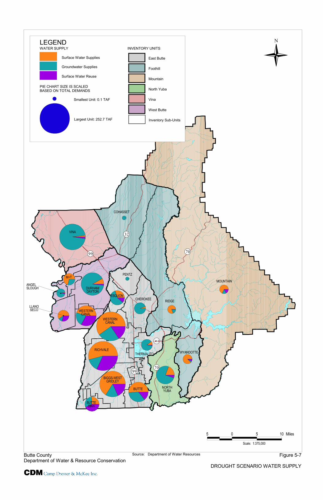
Figure 5-7 shows the composition of supplies for each inventory sub-unit. This figurecan be compared with Figure 5-4, Normal Year Water Supplies, to determine changesduring drought years. Several noteworthy features include:

! There is more groundwater pumping and less surface water. Surface waterdecreases from 55% of supply in normal years to 41% during a drought, andgroundwater increases from 31% to 44%. Surface water reuse stays essentially thesame, going from 14% in a normal year to 15% during a drought.

! In several service areas, surface-water reuse increases in drought years becausethese water suppliers are more careful with the water that can leave their system.By reducing outflows, the water remains in the system for a longer time and isoften reused. However, increased surface water reuse has the potential to degradewater quality.

! Distribution of supplies among the Inventory Units is roughly similar to demands:East Butte is 59% of total supplies, West Butte is 20%, Vina is 12%, North Yuba is6%, Foothill is 2%, and Mountain is 1%.


!"!"!"!" 5-18

Table 5-7Drought Year Supplies (in thousands of acre-feet)


LocalSurfaceWater

FeatherRiver SWP CVP

Ground-water

SurfaceWaterReuse

TotalSupplies

Biggs-West

Gridley 0.0 113.0 0.0 0.0 28.0 29.8 170.8Butte 0.0 50.0 0.0 0.0 34.6 13.4 98.0

Butte Sink 2.1 0.0 0.0 10.8 15.1 21.1 49.1Cherokee 0.0 1.3 0.0 0.0 27.2 0.2 28.7Esquon 15.3 0.0 0.0 0.0 29.8 5.4 50.5Pentz 0.0 0.0 0.0 0.0 0.1 0.0 0.1

Richvale 0.0 118.6 0.0 0.0 30.5 70.2 219.3Thermalito 0.0 2.8 0.0 0.0 24.1 0.4 27.3WesternCanal 3.3 125.1 0.0 0.0 51.8 35.3 215.5

East Butte

Total 20.7 410.8 0.0 10.8 241.2 175.7 859.3Cohasset 0.0 0.0 0.0 0.0 0.4 0.0 0.4

Ridge 9.6 0.0 0.0 0.0 2.1 0.2 11.9Wyandotte 0.0 14.8 0.0 0.0 0.7 1.4 16.9

Foothill

Total 9.6 14.8 0.0 0.0 3.2 1.6 29.2Mountain Mountain 0.0 10.1 0.0 0.0 2.1 2.4 14.6

NorthYuba

NorthYuba 0.0 15.4 0.0 0.0 62.1 3.9 81.4

Vina Vina 0.0 0.0 0.0 3.3 164.8 3.7 171.8Angel

Slough 0.0 0.0 0.0 0.3 12.8 0.5 13.6Durham/Dayton 7.1 3.3 0.0 0.0 118.9 2.9 132.2LlanoSeco 0.0 5.2 0.0 11.1 3.2 7.9 27.4M&T 5.3 4.7 0.0 11.8 8.9 0.0 30.7

WesternCanal 0.0 46.8 0.0 0.0 23.3 34.3 104.4

West Butte

Total 12.4 60.0 0.0 23.2 167.1 45.6 308.3Butte County Total 42.7 511.1 0.0 37.3 640.5 233.0 1,464.6

5.4.3 Net Groundwater ExtractionTable 5-8 indicates deep percolation to groundwater and net groundwater pumpingduring a drought year. Figure 5-8 illustrates these results by inventory sub-unit andcan be compared to Figure 5-5, Normal Year Net Groundwater Pumping. During adrought year, the net groundwater pumping increases significantly in manyinventory sub-units in the valley.


!"!"!"!" 5-19

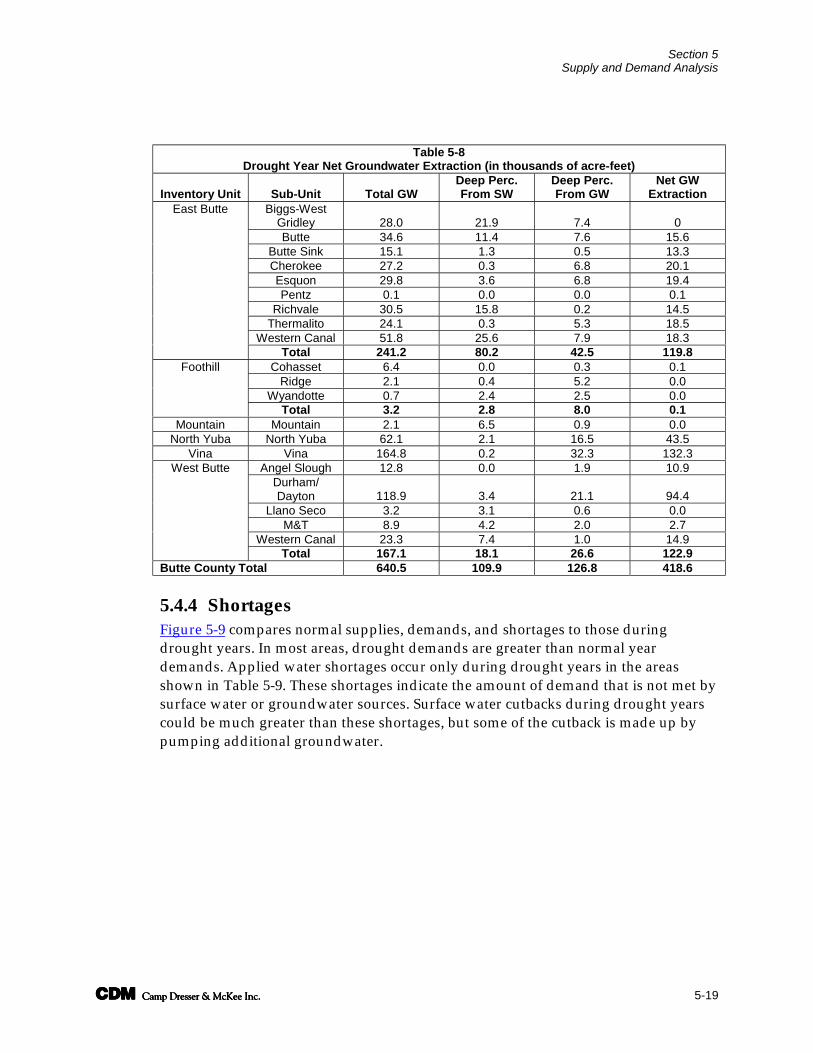
Table 5-8Drought Year Net Groundwater Extraction (in thousands of acre-feet)

Inventory Unit Sub-Unit Total GWDeep Perc.From SW

Deep Perc.From GW

Net GWExtraction

Biggs-WestGridley 28.0 21.9 7.4 0Butte 34.6 11.4 7.6 15.6

Butte Sink 15.1 1.3 0.5 13.3Cherokee 27.2 0.3 6.8 20.1Esquon 29.8 3.6 6.8 19.4Pentz 0.1 0.0 0.0 0.1

Richvale 30.5 15.8 0.2 14.5Thermalito 24.1 0.3 5.3 18.5

Western Canal 51.8 25.6 7.9 18.3

East Butte

Total 241.2 80.2 42.5 119.8Cohasset 6.4 0.0 0.3 0.1

Ridge 2.1 0.4 5.2 0.0Wyandotte 0.7 2.4 2.5 0.0

Foothill

Total 3.2 2.8 8.0 0.1Mountain Mountain 2.1 6.5 0.9 0.0

North Yuba North Yuba 62.1 2.1 16.5 43.5Vina Vina 164.8 0.2 32.3 132.3

Angel Slough 12.8 0.0 1.9 10.9Durham/Dayton 118.9 3.4 21.1 94.4

Llano Seco 3.2 3.1 0.6 0.0M&T 8.9 4.2 2.0 2.7

Western Canal 23.3 7.4 1.0 14.9

West Butte

Total 167.1 18.1 26.6 122.9Butte County Total 640.5 109.9 126.8 418.6

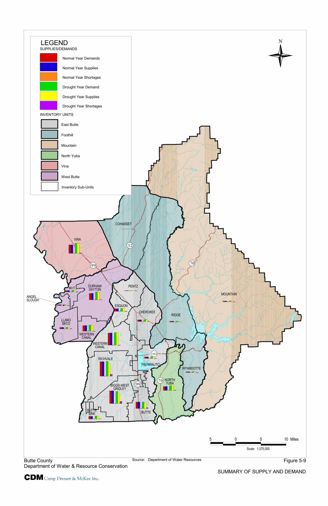
5.4.4 ShortagesFigure 5-9 compares normal supplies, demands, and shortages to those duringdrought years. In most areas, drought demands are greater than normal yeardemands. Applied water shortages occur only during drought years in the areasshown in Table 5-9. These shortages indicate the amount of demand that is not met bysurface water or groundwater sources. Surface water cutbacks during drought yearscould be much greater than these shortages, but some of the cutback is made up bypumping additional groundwater.


!"!"!"!" 5-20

Table 5-9Drought Year Water Shortages


Shortage(TAF)

Total Demand(TAF)

Biggs-West Gridley 37.4 208.2Butte 13.5 111.5

Butte Sink 3.1 52.2Cherokee 3.2 31.9Richvale 33.6 252.9

East Butte

Total 90.8 655.7Cohasset 0.1 0.5

Ridge 1.2 13.1Foothill

Total 1.3 13.6Total 92.1 669.3

Shortages are primarily in the southwest portion of the county. Shortages are definedby lack of supply, which is limited by the groundwater infrastructure available in thesouthwest, not by total water supply.

The water shortage in the Ridge is somewhat different than the other sub-units, and iscaused by a lack of surface water infrastructure. The shortage in Cohasset is due to alack of groundwater depth and infrastructure.

Richvale, Biggs-West Gridley, and Butte are all part of the Joint Water District, whichhas adequate surface water supplies during normal years. Figure 4-2 illustrated thedistribution of wells within the county, and there are not enough wells in these areasto provide groundwater during droughts. During normal years, it is not economicalfor farmers to pump groundwater, so many farmers do not have the necessaryinfrastructure. Shortages only occur in areas that do not receive surface water and donot have the infrastructure to pump groundwater.

5.4.5 Impacts on GroundwaterTable 5-10 illustrates how seasonal groundwater pumping changes the depth ofgroundwater and how this change could impact area wells. Most wells remain belowthe estimated groundwater level during periods of drought.

Estimated additional drawdown was calculated to assess the potential change ingroundwater levels for areas with projected water shortages under the droughtscenario. Shortages result from a lack of wells to extract groundwater from the aquiferand/or a lack of conveyance, adequate supplies of groundwater exist to meet allshortages. Additional drawdown calculations include the total projected shortagevolume without consideration of deep percolation recharge of the additional waters.Estimates of additional drawdown to meet shortages would result in the lowering ofgroundwater levels from three feet in the Cherokee inventory unit to 18 feet in theBiggs West Gridley inventory unit.


!"!"!"!" 5-21

Table 5-10Drought Year Seasonal Groundwater Impacts

% Wells Below GW Level

InventoryUnit

InventorySub-Unit

Avg.Depthto GW

(ft)

EstimatedDrawdown

DuringGrowing

Season (ft) Domestic Irrigation Municipal

AdditionalEstimatedDrawdown

to MeetShortages

Biggs-WestGridley 13 8 100 100 NC 18Butte 13 21 100 100 NC 10

Butte Sink 13 2 NC NC NC 5Cherokee 13 27 100 100 NC 3Esquon 13 30 99.7 100 NC N/APentz 13 1 100 100 NC N/A

Richvale 13 10 100 100 NC 13Thermalito 13 13 100 100 NC N/A

East Butte

WesternCanal 13 17 100 100 NC N/A

NorthYuba North Yuba 37 13 95.4 98.9 NC N/AVina Vina 26 28 98.8 0.6 100 N/A

AngelSlough 22 34 90 NC NC N/A

Durham/Dayton 22 41 97.7 99.6 NC N/A

Llano Seco 22 1 NC NC NC N/AM&T 22 13 NC 100 NC N/A

WestButte

WesternCanal 22 2 NC NC NC N/A

NC – Not Calculated (because well data is not available)N/A – Not Applicable (because sub-unit does not have a shortage)

5.5 LimitationsThe supply and demand inventory was designed to be a tool for decision making andlooks simply at a snapshot in time. There are limitations on how accurate the resultscan be, based on the inputs and the style of analysis.

5.5.1 Data CollectionCollecting additional data could further refine the analysis. The following informationwould be important next steps to continue to improve the understanding of ButteCounty’s water resources:

! Additional groundwater-level data;

! Return flows; and

! Deep percolation.


!"!"!"!" 5-22

5.5.2 AnalysisThe greatest limitation to the inventory was the analysis method. The inventorycreates a snapshot picture of 1 normal year and 1 dry year. However, it cannot displaylinks between years. Most droughts in California include multiple years, so looking at1 drought year does not completely illustrate a drought scenario.

The groundwater analysis in this report is a simple analysis performed to illustratepotential impacts of how supply and demand are distributed. The Butte Basin WaterUsers’ Association is working on a groundwater model that should be a better tool tounderstand the groundwater within the county, and the information in this inventorycan be used as input information for that model.

!"!"!"!"

Figures

P ine Creek

Rock Creek

Mud Cr

eek

Big Chico C

reek Little

Chico

Creek

Butte

Cree

k

Dry C

r eek

W. Br

anch

Feath

er Ri

ver

N. F

ork Fe

ather

River

M. For

k Fea

ther R

iver

Fall River

S. Fork Feather Rive

r

Ange

l Sl ou

gh

Li tt le

Dry

Creek

Honcut

Cree

k

FOOTHILL

MOUNTAINWESTBUTTE

EASTBUTTE

NORTHYUBA

#

VINA

COHASSET

VINA

M+TANGELSLOUGH

#

LLANOSECO

WESTERNCANAL

WESTERNCANAL

DURHAM/DAYTON ESQUON

CHEROKEE RIDGE

PENTZ

MOUNTAIN

WYANDOTTE

NORTHYUBA

THERMALITO

RICHVALE

BIGGS-WEST GRIDLEY

BUTTE

BUTTE SINK

ThermalitoAfterbay

LakeOroville

Sacramento River

Rivers/StreamsLakes

Inventory Units

Inventory Sub-Units

LEGEND

Land UseSubtropicalDeciduous OrchardField CropsGrainIdleNative BarrenNative RiparianNative Vegetation

WaterPastureRiceSemi Ag & IncidentalTruck CropsUrbanVineyard

Scale: 1:375,000

5 0 5 10 Miles

N

Source: Department of Water Resources and Butte County Planning DepartmentButte CountyDepartment of Water & Resource Conservation

Figure 5-1

LAND USE

Figure 5-2

WATER SOURCES

Butte CountyDepartment of Water & Resource Conservation

Source: Department of Water Resources, Butte County Planning Department, and US Bureau of Reclaimation

N

5 0 5 10 MilesScale: 1:375,000

ThermalitoAfterbay

LakeOroville

FOOTHILL

MOUNTAIN

WESTBUTTE

EASTBUTTE

NORTHYUBA

#

VINA

COHASSET

VINA

M+TANGELSLOUGH

#

LLANOSECO

WESTERNCANAL

WESTERNCANAL

DURHAM/DAYTON ESQUON

CHEROKEE RIDGE

PENTZ

MOUNTAIN

WYANDOTTE

NORTHYUBA

THERMALITO

RICHVALE

BIGGS-WEST GRIDLEY

BUTTE

BUTTE SINK

Sacramento River

Honcut

Cree

kL ittle

Dry

Creek

Ange

l Slou

gh

S. Fork Feather Rive

r

Fall River

M. For

k Fea

ther R

iver

N. F

ork F

eather

River

W. Br

anch

Feath

er Ri

v er

Dry C

r eek

Butte

Cree

k

Little

Chico

Creek

Big Chico C

reekMud

Creek

Rock Creek

Pine CreekAngel Slough

Rivers/StreamsLakes

Inventory Sub-Units

Inventory Units

Water SourcesSurface Water SourceMixed Water SourceGroundwater Source

LEGEND

#

"!99 "!70

"!162

"!70

"!32

"!99

Figure 5-3

NORMAL SCENARIO WATER DEMAND


Source: Department of Water Resources

N

5 0 5 10 Miles

Scale: 1:375,000

THERMALITO

CHEROKEE

COHASSET

PENTZ

MOUNTAIN

RIDGE

WYANDOTTE

NORTHYUBA

BUTTESINK

BUTTE

RICHVALE

ESQUON

WESTERNCANAL

WESTERNCANAL

DURHAM/DAYTON

#

#

LLANOSECO

ANGELSLOUGH

M+T

VINA

INVENTORY UNITS

East Butte

Foothill

Mountain

North Yuba

Vina

West Butte

Inventory Sub-Units

WATER DEMANDS

Agricultural Demand

Municipal and Industrial Demand

Environmental Demand

Conveyance Losses

Smallest Unit: 0.1 TAF

Largest Unit: 247 TAF

PIE CHART SIZE IS SCALEDBASED ON TOTAL DEMANDS

LEGEND

BIGGS-WESTGRIDLEY

"!99 "!70

"!162

"!70

"!32

"!99

Scale: 1:375,000

5 0 5 10 Miles

N

Source: Department of Water ResourcesButte CountyDepartment of Water & Resource Conservation

Figure 5-4

NORMAL SCENARIO WATER SUPPLY

THERMALITO

CHEROKEE

COHASSET

PENTZ

MOUNTAIN

RIDGE

WYANDOTTE

NORTHYUBA

BUTTESINK

BUTTE

RICHVALE

ESQUON

WESTERNCANAL

WESTERNCANAL

DURHAM/DAYTON

LLANOSECO

ANGELSLOUGH

M+T

VINA

#

#

Surface Water Supplies

Groundwater Supplies

Surface Water Reuse

WATER SUPPLY


Largest Unit: 247 TAF


INVENTORY UNITS

East Butte

Foothill

Mountain

North Yuba

Vina

West Butte

Inventory Sub-Units

LEGEND

BIGGS-WESTGRIDLEY

WESTERNCANAL

BUTTE SINK

BIGGS-WESTGRIDLEY

DURHAM/DAYTON

CHEROKEE

PENTZ

ESQUON

WESTERNCANAL

RICHVALE

THERMALITO

BUTTE

M+TANGELSLOUGH

#

LLANOSECO

WYANDOTTE

NORTHYUBA

MOUNTAIN

RIDGE

COHASSET

VINA



N

4 0 4 8 Miles

Scale: 1:500,000

LEGENDNet Groundwater Pumping (TAF)

01 - 1415 - 2223 - 4445 - 132

Figure 5-5

NORMAL NET GROUNDWATER EXTRACTION

#

#

#

#

#

#

#

#

#

#

#

#

#

#

#

#

##

#

#

"!99 "!70

"!162

"!70

"!32

"!99

Figure 5-6

DROUGHT SCENARIO WATER DEMAND



N

5 0 5 10 Miles

Scale: 1:375,000

INVENTORY UNITS

East Butte

Foothill

Mountain

North Yuba

Vina

West Butte

Inventory Sub-Units

Agricultural Demand

Municipal and Industrial Demand

Environmental Demand

Conveyance Losses

WATER DEMANDS


Largest Unit: 252.7 TAF


LEGEND

VINA

M+T

ANGELSLOUGH

LLANOSECO

#

#

DURHAM/DAYTON

WESTERNCANAL

WESTERNCANAL

ESQUON

RICHVALE

BUTTE

BUTTESINK

NORTHYUBA

WYANDOTTE

RIDGE

MOUNTAINPENTZ

COHASSET

CHEROKEE

THERMALITO

BIGGS-WESTGRIDLEY

"!99 "!70

"!162

"!70

"!32

"!99

Figure 5-7

DROUGHT SCENARIO WATER SUPPLY



N

5 0 5 10 Miles

Scale: 1:375,000

Surface Water Supplies

Groundwater Supplies

Surface Water Reuse

WATER SUPPLY


Largest Unit: 252.7 TAF


INVENTORY UNITS

East Butte

Foothill

Mountain

North Yuba

Vina

West Butte

Inventory Sub-Units

LEGEND

THERMALITO

CHEROKEE

COHASSET

PENTZMOUNTAIN

RIDGE

WYANDOTTE

NORTHYUBA

BUTTESINK

BUTTE

RICHVALE

ESQUON

WESTERNCANAL

WESTERNCANAL

DURHAM/DAYTON#

#

LLANOSECO

ANGELSLOUGH

M+T

VINA

BIGGS-WESTGRIDLEY

VINA

COHASSET

RIDGE

MOUNTAIN

NORTHYUBA

WYANDOTTE

LLANOSECO

ANGELSLOUGH

#

M+T

BUTTE

THERMALITO

RICHVALE

WESTERNCANAL

ESQUON

PENTZ

CHEROKEE

DURHAM/DAYTON

BIGGS-WESTGRIDLEY

BUTTE SINK

WESTERNCANAL

Scale: 1:500,000

4 0 4 8 Miles

N

Source: Department of Water Resources Figure 5-8

DROUGHT NET GROUNDWATER EXTRACTION


LEGENDNet Groundwater Pumping (TAF)

01 - 1415 - 2223 - 4445 - 132

"!99 "!70

"!162

"!70

"!32

"!99

Figure 5-9

SUMMARY OF SUPPLY AND DEMAND



N

5 0 5 10 Miles

Scale: 1:375,000

INVENTORY UNITS

East Butte

Foothill

Mountain

North Yuba

Vina

West Butte

Inventory Sub-Units

SUPPLIES/DEMANDS

Normal Year Supplies

Normal Year Demands

Normal Year Shortages

Drought Year Demand

Drought Year Supplies

Drought Year Shortages

LEGEND

THERMALITO

CHEROKEE

COHASSET

PENTZ

MOUNTAIN

RIDGE

WYANDOTTE

NORTHYUBA

BUTTESINK BUTTE

BIGGS-WESTGRIDLEY

RICHVALE

ESQUON

WESTERNCANAL

WESTERNCANAL

DURHAM/DAYTON

#

LLANOSECO

ANGELSLOUGH

M+T

VINA

Documents

Section 5 Supply and Demand Analysis - Butte County > … · · 2013-12-12Section 5 Supply and Demand Analysis ... 5.1.1 Water Demand Methodology The individual system and inter-system