ENGR 202 – Electrical Fundamentals II

SECTION 4: SECOND-ORDER TRANSIENT RESPONSE

K. Webb ENGR 202

Introduction2

K. Webb ENGR 202

3

Second-Order Circuits

In this and the previous section of notes, we consider second-order RLC circuits from two distinct perspectives: Frequency-domain Second-order, RLC filters

Time-domain Second-order, RLC step response

K. Webb ENGR 202

Transient Response of Second-Order Circuits

4

K. Webb ENGR 202

5

Second-Order Transient Response

In ENGR 201 we looked at the transient response of first-order RC and RL circuits Applied KVL Governing differential equation

Solved the ODE Expression for the step response

For second-order circuits, process is the same: Apply KVL Second-order ODE

Solve the ODE Second-order step response

K. Webb ENGR 202

6

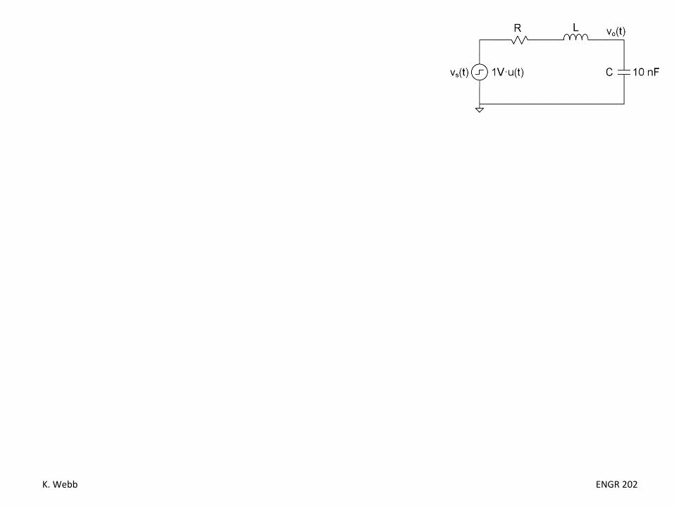
Step Response of RLC Circuit

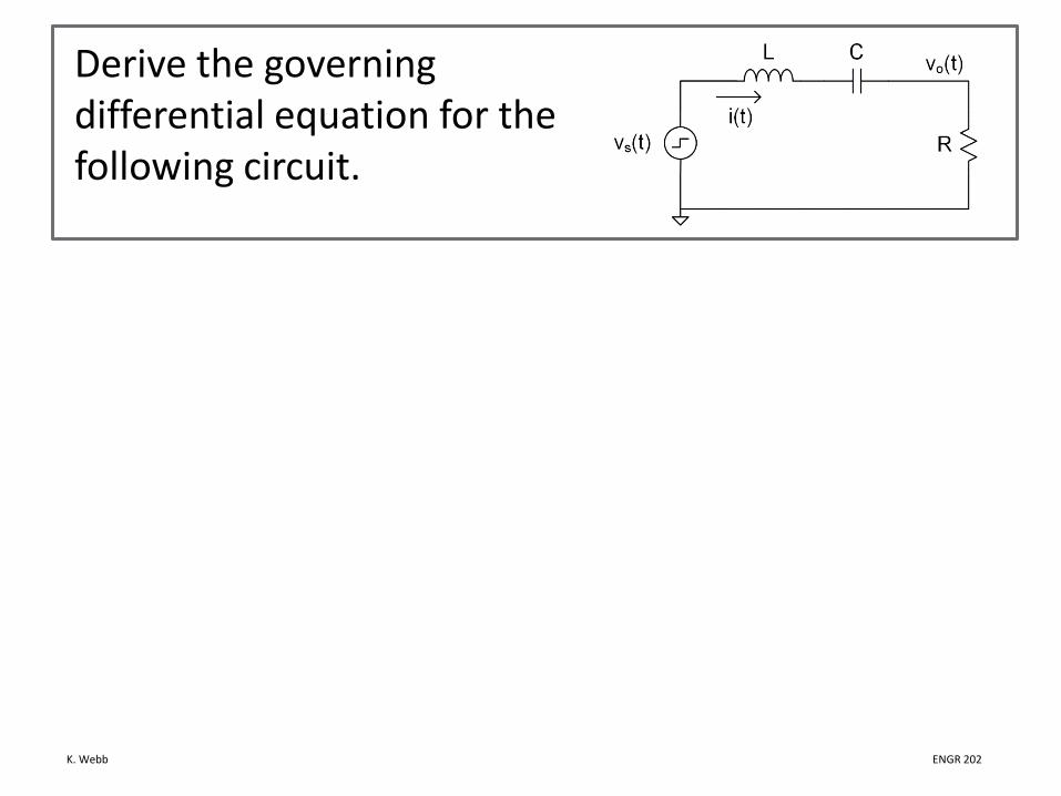
Determine the response of the following RLC circuit Source is a voltage step: 𝑣𝑣𝑠𝑠 𝑡𝑡 = 1𝑉𝑉 ⋅ 𝑢𝑢 𝑡𝑡 Output is the voltage across the capacitor

Apply KVL around the loop

𝑣𝑣𝑠𝑠 𝑡𝑡 − 𝑖𝑖 𝑡𝑡 𝑅𝑅 − 𝐿𝐿𝑑𝑑𝑖𝑖𝑑𝑑𝑡𝑡− 𝑣𝑣𝑜𝑜 𝑡𝑡 = 0

Want an ODE in terms of 𝑣𝑣𝑜𝑜 𝑡𝑡 Need to eliminate 𝑖𝑖 𝑡𝑡 Can express 𝑖𝑖 𝑡𝑡 in terms of the output voltage:

𝑖𝑖 𝑡𝑡 = 𝐶𝐶 𝑑𝑑𝑣𝑣𝑜𝑜𝑑𝑑𝑑𝑑

so, 𝑑𝑑𝑑𝑑𝑑𝑑𝑑𝑑

= 𝐶𝐶 𝑑𝑑2𝑣𝑣0𝑑𝑑𝑑𝑑2

K. Webb ENGR 202

7

Step Response of RLC Circuit

Substituting in the expression for current, the KVL equation becomes

𝑣𝑣𝑠𝑠 𝑡𝑡 − 𝐶𝐶𝑑𝑑𝑣𝑣𝑜𝑜𝑑𝑑𝑡𝑡

𝑅𝑅 − 𝐿𝐿𝐶𝐶𝑑𝑑2𝑣𝑣𝑜𝑜𝑑𝑑𝑡𝑡2 − 𝑣𝑣𝑜𝑜 𝑡𝑡 = 0

Rearranging gives the governing second-order ODE:

𝑑𝑑2𝑣𝑣𝑜𝑜𝑑𝑑𝑡𝑡2 +

𝑅𝑅𝐿𝐿𝑑𝑑𝑣𝑣𝑜𝑜𝑑𝑑𝑡𝑡 +

1𝐿𝐿𝐶𝐶 𝑣𝑣𝑜𝑜 𝑡𝑡 =

1𝐿𝐿𝐶𝐶 𝑣𝑣𝑠𝑠 𝑡𝑡

A second-order, linear, non-homogeneous, ordinary differential equation Non-homogeneous, so solve in two parts

1) Find the complementary solution to the homogeneous equation2) Find the particular solution for the step input

General solution will be the sum of the two individual solutions:

𝑣𝑣𝑜𝑜 𝑡𝑡 = 𝑣𝑣𝑜𝑜𝑜𝑜 𝑡𝑡 + 𝑣𝑣𝑜𝑜𝑜𝑜 𝑡𝑡

K. Webb ENGR 202

Complementary Solution8

K. Webb ENGR 202

9

Complementary Solution – 𝑣𝑣𝑜𝑜𝑜𝑜 𝑡𝑡 The homogeneous equation is obtained by setting the forcing

function (input) to zero

𝑑𝑑2𝑣𝑣𝑜𝑜𝑑𝑑𝑡𝑡2

+𝑅𝑅𝐿𝐿𝑑𝑑𝑣𝑣𝑜𝑜𝑑𝑑𝑡𝑡

+1𝐿𝐿𝐶𝐶

𝑣𝑣𝑜𝑜 𝑡𝑡 = 0

For an ODE of this form, we assume a solution of the form

𝑣𝑣𝑜𝑜𝑜𝑜 𝑡𝑡 = 𝑒𝑒𝑠𝑠𝑑𝑑

Where 𝑠𝑠 is an unknown complex value. Then

𝑑𝑑𝑣𝑣𝑜𝑜𝑜𝑜𝑑𝑑𝑑𝑑

= 𝑠𝑠𝑒𝑒𝑠𝑠𝑑𝑑 and 𝑑𝑑2𝑣𝑣𝑜𝑜𝑜𝑜𝑑𝑑𝑑𝑑2

= 𝑠𝑠2𝑒𝑒𝑠𝑠𝑑𝑑

Substituting back into the homogeneous ODE yields the characteristic equation

𝑠𝑠2 +𝑅𝑅𝐿𝐿𝑠𝑠 +

1𝐿𝐿𝐶𝐶

= 0

K. Webb ENGR 202

10

Complementary Solution – 𝑣𝑣𝑜𝑜𝑜𝑜 𝑡𝑡

𝑠𝑠2 +𝑅𝑅𝐿𝐿𝑠𝑠 +

1𝐿𝐿𝐶𝐶

= 0

The characteristic equation can be rewritten as

𝑠𝑠2 + 2𝛼𝛼𝑠𝑠 + 𝜔𝜔𝑜𝑜2 = 0or

𝑠𝑠2 + 2𝜁𝜁𝜔𝜔𝑜𝑜𝑠𝑠 + 𝜔𝜔𝑜𝑜2 = 0

The roots of the characteristic equation (also called poles) tell us about the: Form of the complementary solution Nature of the response

These roots (or poles) are

𝑠𝑠1 = −𝛼𝛼 + 𝛼𝛼2 − 𝜔𝜔02 , 𝑠𝑠2 = −𝛼𝛼 − 𝛼𝛼2 − 𝜔𝜔02

where𝛼𝛼 = 𝑅𝑅

2𝐿𝐿and 𝜔𝜔0 = 1

𝐿𝐿𝐿𝐿

K. Webb ENGR 202

11

Complementary Solution – 𝑣𝑣𝑜𝑜𝑜𝑜 𝑡𝑡

We’ve said we can write the characteristic equation as𝑠𝑠2 + 2𝛼𝛼𝑠𝑠 + 𝜔𝜔0

2 = 0or

𝑠𝑠2 + 2𝜁𝜁𝜔𝜔0𝑠𝑠 + 𝜔𝜔02 = 0

𝑇𝑇he damping ratio, 𝜁𝜁, can be defined as

𝜁𝜁 =𝛼𝛼𝜔𝜔0

A few key points: 𝜔𝜔0 is the resonant frequency 𝜁𝜁 characterizes the nature (sharpness) of the resonance Both are related to the roots of the characteristic equation

K. Webb ENGR 202

12

Complementary Solution – 𝑣𝑣𝑜𝑜𝑜𝑜 𝑡𝑡 Complementary solution has the same form as that of a first-order

circuit: 𝑣𝑣𝑜𝑜𝑜𝑜 𝑡𝑡 = 𝑒𝑒𝑠𝑠𝑑𝑑

𝑠𝑠 is the roots of the characteristic equation Now two values – identical or distinct May be complex

Form of the solution depends on the values of 𝑠𝑠 Can be characterized in terms of the value of 𝜁𝜁:

𝜻𝜻 > 𝟏𝟏 – over-damped case: 𝑣𝑣𝑜𝑜𝑜𝑜 𝑡𝑡 = 𝐾𝐾1𝑒𝑒𝑠𝑠1𝑑𝑑 + 𝐾𝐾2𝑒𝑒𝑠𝑠2𝑑𝑑

𝜻𝜻 = 𝟏𝟏 – critically-damped case:𝑣𝑣𝑜𝑜𝑜𝑜 𝑡𝑡 = 𝐾𝐾1𝑒𝑒𝑠𝑠1𝑑𝑑 + 𝐾𝐾2𝑡𝑡𝑒𝑒𝑠𝑠1𝑑𝑑

𝜻𝜻 < 𝟏𝟏 – under-damped case: 𝑣𝑣𝑜𝑜𝑜𝑜 𝑡𝑡 = 𝐾𝐾1𝑒𝑒−𝛼𝛼𝑑𝑑 cos 𝜔𝜔𝑑𝑑𝑡𝑡 + 𝐾𝐾2𝑒𝑒−𝛼𝛼𝑑𝑑 sin 𝜔𝜔𝑑𝑑𝑡𝑡

K. Webb ENGR 202

13

Over-Damped RLC Circuit – 𝜁𝜁 > 1 Roots of the characteristic equation are

𝑠𝑠1 = −𝛼𝛼 + 𝛼𝛼2 − 𝜔𝜔02 , 𝑠𝑠1 = −𝛼𝛼 + 𝛼𝛼2 − 𝜔𝜔02

These are related to the damping ratio as

𝜁𝜁 =𝛼𝛼𝜔𝜔0

If 𝜁𝜁 > 1, then 𝛼𝛼 > 𝜔𝜔0 𝛼𝛼2 − 𝜔𝜔0

2 > 0 – i.e., the discriminant is positive 𝑠𝑠1 and 𝑠𝑠2 are real and distinct

Complimentary solution has the following form

𝑣𝑣𝑜𝑜𝑜𝑜 𝑡𝑡 = 𝐾𝐾1𝑒𝑒𝑠𝑠1𝑑𝑑 + 𝐾𝐾2𝑒𝑒𝑠𝑠2𝑑𝑑

Recall that 𝜁𝜁 > 1 (actually, 𝜁𝜁 ≥ 0.707) corresponded to no peaking in the frequency domain

K. Webb ENGR 202

14

Critically-Damped RLC Circuit – 𝜁𝜁 = 1

𝑠𝑠1 = −𝛼𝛼 + 𝛼𝛼2 − 𝜔𝜔02 , 𝑠𝑠1 = −𝛼𝛼 + 𝛼𝛼2 − 𝜔𝜔02

If 𝜁𝜁 = 1, then 𝛼𝛼 = 𝜔𝜔0 𝛼𝛼2 − 𝜔𝜔02 = 0 – i.e., the discriminant is zero 𝑠𝑠1 and 𝑠𝑠2 are real and identical

Complimentary solution has the following form

𝑣𝑣𝑜𝑜𝑜𝑜 𝑡𝑡 = 𝐾𝐾1𝑒𝑒𝑠𝑠1𝑑𝑑 + 𝐾𝐾2𝑡𝑡𝑒𝑒𝑠𝑠1𝑑𝑑

This is the lowest value of 𝜁𝜁 for which the step response is monotonic Constantly increasing No overshoot

K. Webb ENGR 202

15

Under-Damped RLC Circuit – 𝜁𝜁 < 1 If 𝜁𝜁 < 1, then

𝛼𝛼 < 𝜔𝜔0 𝛼𝛼2 − 𝜔𝜔02 < 0 – i.e., the discriminant is negative 𝑠𝑠1 and 𝑠𝑠2 are a complex conjugate pair

Complimentary solution has the following form

𝑣𝑣𝑜𝑜𝑜𝑜 𝑡𝑡 = 𝐾𝐾1𝑒𝑒−𝛼𝛼𝑑𝑑 cos 𝜔𝜔𝑑𝑑𝑡𝑡 + 𝐾𝐾2𝑒𝑒−𝛼𝛼𝑑𝑑 sin 𝜔𝜔𝑑𝑑𝑡𝑡

𝜔𝜔𝑑𝑑 is the damped natural frequency

𝜔𝜔𝑑𝑑 = 𝜔𝜔02 − 𝛼𝛼2 = 𝜔𝜔0 1 − 𝜁𝜁2

Response now contains damped sinusoidal components Will exhibit overshoot Possible ringing

K. Webb ENGR 202

16

Damping Cases – Geometric Interpretation

Roots of characteristic equation (system poles) are, in general, complex Can plot them in the complex plane Pole locations tell us a lot about the nature of the response

Speed – risetime, settling time Overshoot, ringing

ζ < 1 – underdampedζ = 1 – critically-dampedζ > 1 – overdampedCase 1: Case 2: Case 3:

K. Webb ENGR 202

17

Under-Damped Case – 𝛼𝛼, 𝜁𝜁, and 𝜔𝜔0

Under-damped case – 𝜁𝜁 < 1 Roots are a complex-conjugate pair

𝑠𝑠1,2 = −𝛼𝛼 ± 𝑗𝑗𝜔𝜔𝑑𝑑

𝛼𝛼 is the real part 𝜔𝜔𝑑𝑑 is the imaginary part The magnitude of the root is

𝜔𝜔0 = 𝛼𝛼2 + 𝜔𝜔𝑑𝑑2

Angle between imaginary axis and vector to the poles is related to damping

𝜁𝜁 =𝛼𝛼𝜔𝜔0

= sin 𝜃𝜃

K. Webb ENGR 202

Particular Solution18

K. Webb ENGR 202

19

Particular solution – 𝑣𝑣𝑜𝑜𝑜𝑜 𝑡𝑡

General solution for the RLC step response is the sum of the complementary and particular solutions

𝑣𝑣𝑜𝑜 𝑡𝑡 = 𝑣𝑣𝑜𝑜𝑜𝑜 𝑡𝑡 + 𝑣𝑣𝑜𝑜𝑜𝑜 𝑡𝑡

We now have the complementary solution with two unknown constants, 𝐾𝐾1 and 𝐾𝐾2 Constants to be determined later through application of

initial conditions Next, determine the particular solution, 𝑣𝑣𝑜𝑜𝑜𝑜 𝑡𝑡

For a circuit driven by a step input, this is simply the circuit’s steady-state response

𝑣𝑣𝑜𝑜𝑜𝑜 𝑡𝑡 = 𝑣𝑣𝑜𝑜 𝑡𝑡 → ∞

K. Webb ENGR 202

20

Particular solution – 𝑣𝑣𝑜𝑜𝑜𝑜 𝑡𝑡

Particular solution is the circuit’s steady-state response Inductor → short Capacitor → open

𝑣𝑣𝑜𝑜𝑜𝑜 𝑡𝑡 = 𝑣𝑣𝑜𝑜 𝑡𝑡 → ∞ = 𝑣𝑣𝑠𝑠 𝑡𝑡 > 0

For a unit step input, the particular solution is𝑣𝑣𝑜𝑜𝑜𝑜 𝑡𝑡 = 1 𝑉𝑉

K. Webb ENGR 202

Example Problems21

K. Webb ENGR 202

Derive the governing differential equation for the following circuit.

K. Webb ENGR 202

K. Webb ENGR 202

Determine: Damping ratio Damping case Characteristic equation Poles

K. Webb ENGR 202

K. Webb ENGR 202

Determine: Initial conditions Particular solution

For𝑣𝑣𝑠𝑠 𝑡𝑡 = −1𝑉𝑉 ⋅ 𝑢𝑢 𝑡𝑡 + 2𝑉𝑉

K. Webb ENGR 202

K. Webb ENGR 202

K. Webb ENGR 202

K. Webb ENGR 202

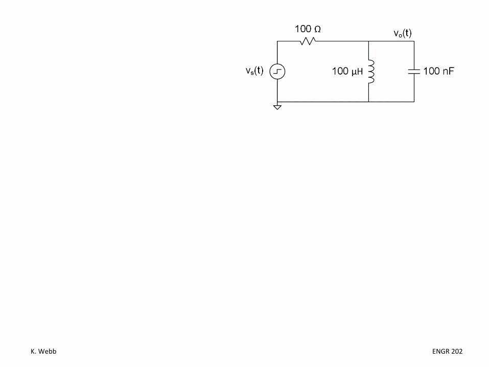
Derive the governing differential equation for the following circuit.

K. Webb ENGR 202

K. Webb ENGR 202

Over-Damped Circuit Response32

K. Webb ENGR 202

33

RLC Step Response – Example 1

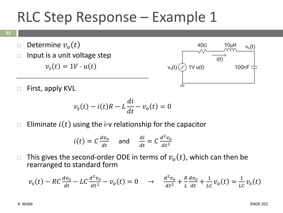
Determine 𝑣𝑣𝑜𝑜 𝑡𝑡 Input is a unit voltage step

𝑣𝑣𝑠𝑠 𝑡𝑡 = 1𝑉𝑉 ⋅ 𝑢𝑢 𝑡𝑡

First, apply KVL

𝑣𝑣𝑠𝑠 𝑡𝑡 − 𝑖𝑖 𝑡𝑡 𝑅𝑅 − 𝐿𝐿𝑑𝑑𝑖𝑖𝑑𝑑𝑡𝑡 − 𝑣𝑣𝑜𝑜 𝑡𝑡 = 0

Eliminate 𝑖𝑖 𝑡𝑡 using the i-v relationship for the capacitor

𝑖𝑖 𝑡𝑡 = 𝐶𝐶 𝑑𝑑𝑣𝑣𝑜𝑜𝑑𝑑𝑑𝑑

and 𝑑𝑑𝑑𝑑𝑑𝑑𝑑𝑑

= 𝐶𝐶 𝑑𝑑2𝑣𝑣𝑜𝑜𝑑𝑑𝑑𝑑2

This gives the second-order ODE in terms of 𝑣𝑣𝑜𝑜 𝑡𝑡 , which can then be rearranged to standard form

𝑣𝑣𝑠𝑠 𝑡𝑡 − 𝑅𝑅𝐶𝐶 𝑑𝑑𝑣𝑣𝑜𝑜𝑑𝑑𝑑𝑑

− 𝐿𝐿𝐶𝐶 𝑑𝑑2𝑣𝑣𝑜𝑜𝑑𝑑𝑑𝑑2

− 𝑣𝑣𝑜𝑜 𝑡𝑡 = 0 → 𝑑𝑑2𝑣𝑣𝑜𝑜𝑑𝑑𝑑𝑑2

+ 𝑅𝑅𝐿𝐿𝑑𝑑𝑣𝑣𝑜𝑜𝑑𝑑𝑑𝑑

+ 1𝐿𝐿𝐿𝐿𝑣𝑣𝑜𝑜 𝑡𝑡 = 1

𝐿𝐿𝐿𝐿𝑣𝑣𝑠𝑠 𝑡𝑡

K. Webb ENGR 202

34

RLC Step Response – Example 1

Find the complementary solution, 𝑣𝑣𝑜𝑜𝑜𝑜 𝑡𝑡 The homogeneous equation

𝑑𝑑2𝑣𝑣𝑜𝑜𝑑𝑑𝑡𝑡2 +

𝑅𝑅𝐿𝐿𝑑𝑑𝑣𝑣𝑜𝑜𝑑𝑑𝑡𝑡

+1𝐿𝐿𝐶𝐶

𝑣𝑣𝑜𝑜 𝑡𝑡 = 0

The characteristic equation

𝑠𝑠2 +𝑅𝑅𝐿𝐿 𝑠𝑠 +

1𝐿𝐿𝐶𝐶 = 0

This can be rewritten as𝑠𝑠2 + 2𝛼𝛼𝑠𝑠 + 𝜔𝜔0

2 = 0where

𝛼𝛼 =𝑅𝑅2𝐿𝐿 =

40 Ω2 ⋅ 10 𝜇𝜇𝜇𝜇 = 2 × 106

𝑟𝑟𝑟𝑟𝑑𝑑𝑠𝑠𝑒𝑒𝑠𝑠

and

𝜔𝜔0 =1𝐿𝐿𝐶𝐶

=1

10 𝜇𝜇𝜇𝜇 ⋅ 100 𝑛𝑛𝑛𝑛= 1 × 106

𝑟𝑟𝑟𝑟𝑑𝑑𝑠𝑠𝑒𝑒𝑠𝑠

K. Webb ENGR 202

35

RLC Step Response – Example 1

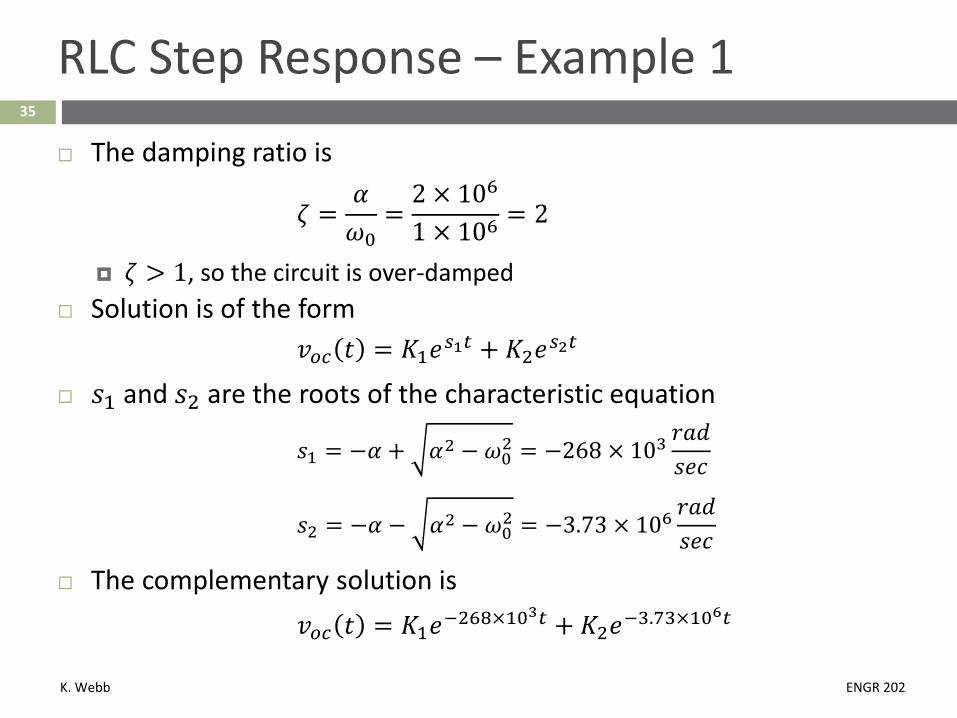
The damping ratio is

𝜁𝜁 =𝛼𝛼𝜔𝜔0

=2 × 106

1 × 106= 2

𝜁𝜁 > 1, so the circuit is over-damped Solution is of the form

𝑣𝑣𝑜𝑜𝑜𝑜 𝑡𝑡 = 𝐾𝐾1𝑒𝑒𝑠𝑠1𝑑𝑑 + 𝐾𝐾2𝑒𝑒𝑠𝑠2𝑑𝑑

𝑠𝑠1 and 𝑠𝑠2 are the roots of the characteristic equation

𝑠𝑠1 = −𝛼𝛼 + 𝛼𝛼2 − 𝜔𝜔02 = −268 × 103𝑟𝑟𝑟𝑟𝑑𝑑𝑠𝑠𝑒𝑒𝑠𝑠

𝑠𝑠2 = −𝛼𝛼 − 𝛼𝛼2 − 𝜔𝜔02 = −3.73 × 106𝑟𝑟𝑟𝑟𝑑𝑑𝑠𝑠𝑒𝑒𝑠𝑠

The complementary solution is 𝑣𝑣𝑜𝑜𝑜𝑜 𝑡𝑡 = 𝐾𝐾1𝑒𝑒−268×103𝑑𝑑 + 𝐾𝐾2𝑒𝑒−3.73×106𝑑𝑑

K. Webb ENGR 202

36

RLC Step Response – Example 1

The particular solution is the circuit’s steady-state solution

Steady-state equivalent circuit: Capacitor → open Inductor → short

So, the particular solution is

𝑣𝑣𝑜𝑜𝑜𝑜 𝑡𝑡 = 1 𝑉𝑉

The general solution:

𝑣𝑣𝑜𝑜 𝑡𝑡 = 𝑣𝑣𝑜𝑜𝑜𝑜 𝑡𝑡 + 𝑣𝑣𝑜𝑜𝑜𝑜 𝑡𝑡

𝑣𝑣𝑜𝑜 𝑡𝑡 = 𝐾𝐾1𝑒𝑒−268×103𝑑𝑑 + 𝐾𝐾2𝑒𝑒−3.73×106𝑑𝑑 + 1 𝑉𝑉

Next, we’ll apply initial conditions to determine the unknown coefficients, 𝐾𝐾1 and 𝐾𝐾2

K. Webb ENGR 202

37

RLC Step Response – Example 1

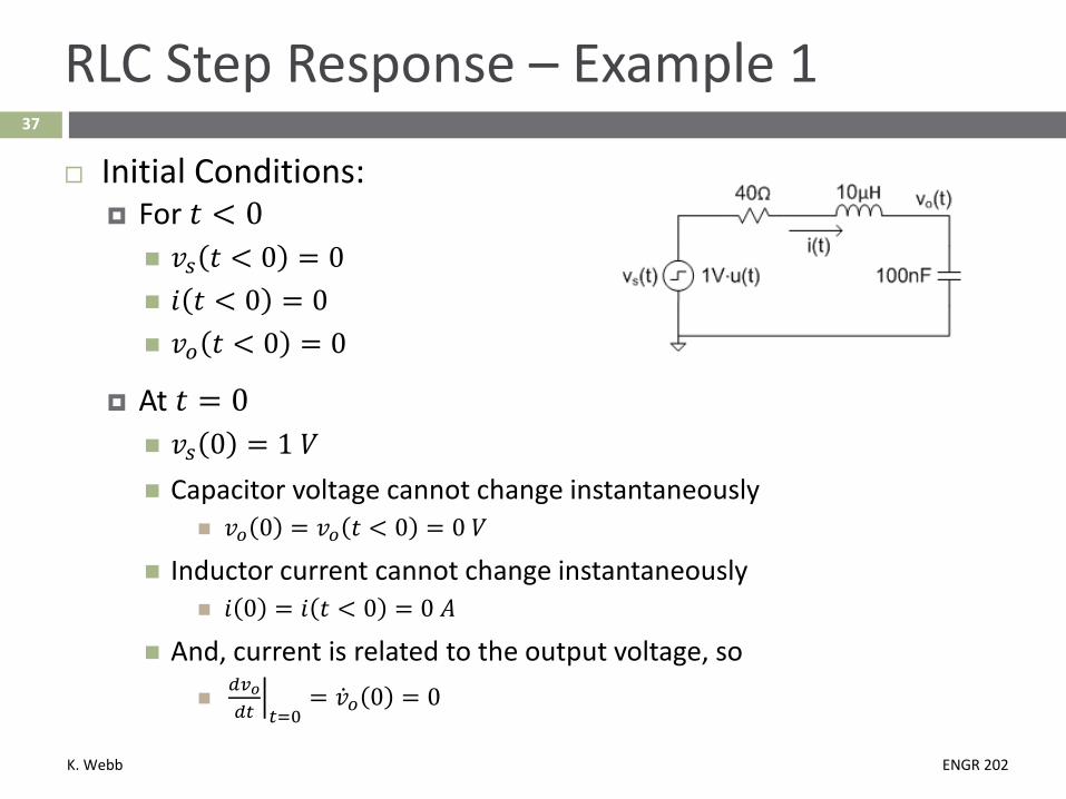
Initial Conditions: For 𝑡𝑡 < 0 𝑣𝑣𝑠𝑠 𝑡𝑡 < 0 = 0 𝑖𝑖 𝑡𝑡 < 0 = 0 𝑣𝑣𝑜𝑜 𝑡𝑡 < 0 = 0

At 𝑡𝑡 = 0 𝑣𝑣𝑠𝑠 0 = 1 𝑉𝑉 Capacitor voltage cannot change instantaneously

𝑣𝑣𝑜𝑜 0 = 𝑣𝑣𝑜𝑜 𝑡𝑡 < 0 = 0 𝑉𝑉

Inductor current cannot change instantaneously 𝑖𝑖 0 = 𝑖𝑖 𝑡𝑡 < 0 = 0 𝐴𝐴

And, current is related to the output voltage, so �𝑑𝑑𝑣𝑣𝑜𝑜

𝑑𝑑𝑑𝑑 𝑑𝑑=0= �̇�𝑣𝑜𝑜 0 = 0

K. Webb ENGR 202

38

RLC Step Response – Example 1

The two initial conditions are:𝑣𝑣𝑜𝑜 0 = 0 (1)

�̇�𝑣𝑜𝑜 0 = 0 (2)

Use the initial conditions to determine 𝐾𝐾1 and 𝐾𝐾2 Applying the first initial condition

𝑣𝑣𝑜𝑜 𝑡𝑡 = 𝐾𝐾1𝑒𝑒𝑠𝑠1𝑑𝑑 + 𝐾𝐾2𝑒𝑒𝑠𝑠2𝑑𝑑 + 1 𝑉𝑉

𝑣𝑣𝑜𝑜 0 = 𝐾𝐾1 + 𝐾𝐾2 + 1 𝑉𝑉 = 0

𝐾𝐾2 = −𝐾𝐾1 − 1 𝑉𝑉 (3)

Applying the second initial condition�̇�𝑣𝑜𝑜 𝑡𝑡 = 𝑠𝑠1𝐾𝐾1𝑒𝑒𝑠𝑠1𝑑𝑑 + 𝑠𝑠2𝐾𝐾2𝑒𝑒𝑠𝑠2𝑑𝑑

�̇�𝑣𝑜𝑜 0 = 𝑠𝑠1𝐾𝐾1 + 𝑠𝑠2𝐾𝐾2 = 0 (4)

K. Webb ENGR 202

39

RLC Step Response – Example 1

Substituting (3) into (4)𝑠𝑠1𝐾𝐾1 − 𝑠𝑠2 𝐾𝐾1 + 1 𝑉𝑉 = 0

𝐾𝐾1 𝑠𝑠1 − 𝑠𝑠2 = 𝑠𝑠2 ⋅ 1 𝑉𝑉

𝐾𝐾1 =𝑠𝑠2

𝑠𝑠1 − 𝑠𝑠2⋅ 1 𝑉𝑉 = −1.08 𝑉𝑉

Substituting the value of 𝐾𝐾1 back into (3) 𝐾𝐾2 = −𝐾𝐾1 − 1 𝑉𝑉 = 0.08 𝑉𝑉

The step response for this over-damped RLC circuit is𝑣𝑣𝑜𝑜 𝑡𝑡 = −1.08 𝑉𝑉 ⋅ 𝑒𝑒𝑠𝑠1𝑑𝑑 + 0.08 𝑉𝑉 ⋅ 𝑒𝑒𝑠𝑠2𝑑𝑑 + 1 𝑉𝑉

𝑣𝑣𝑜𝑜 𝑡𝑡 = −1.08 𝑉𝑉 ⋅ 𝑒𝑒−268×103𝑑𝑑 + 0.08 𝑉𝑉 ⋅ 𝑒𝑒−3.73×106𝑑𝑑 + 1 𝑉𝑉

K. Webb ENGR 202

40

RLC Step Response – Example 1

Similar to first-order response Sum of two decaying

exponentials Monotonic increase

to final value Initial slope differs

from first-order response Increases after 𝑡𝑡 = 0

𝑣𝑣𝑜𝑜 𝑡𝑡 = −1.08 𝑉𝑉 ⋅ 𝑒𝑒−268×103𝑑𝑑 + 0.08 𝑉𝑉 ⋅ 𝑒𝑒−3.73×106𝑑𝑑 + 1 𝑉𝑉

K. Webb ENGR 202

Critically-Damped Circuit Response41

K. Webb ENGR 202

42

RLC Step Response – Example 2

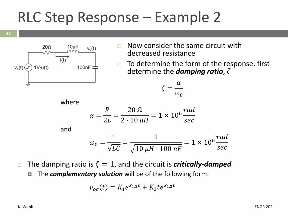
Now consider the same circuit with decreased resistance

To determine the form of the response, first determine the damping ratio, 𝜁𝜁

𝜁𝜁 =𝛼𝛼𝜔𝜔0

where

𝛼𝛼 =𝑅𝑅2𝐿𝐿 =

20 Ω2 ⋅ 10 𝜇𝜇𝜇𝜇 = 1 × 106

𝑟𝑟𝑟𝑟𝑑𝑑𝑠𝑠𝑒𝑒𝑠𝑠

and

𝜔𝜔0 =1𝐿𝐿𝐶𝐶

=1

10 𝜇𝜇𝜇𝜇 ⋅ 100 𝑛𝑛𝑛𝑛= 1 × 106

𝑟𝑟𝑟𝑟𝑑𝑑𝑠𝑠𝑒𝑒𝑠𝑠

The damping ratio is 𝜁𝜁 = 1, and the circuit is critically-damped The complementary solution will be of the following form:

𝑣𝑣𝑜𝑜𝑜𝑜 𝑡𝑡 = 𝐾𝐾1𝑒𝑒𝑠𝑠1,2𝑑𝑑 + 𝐾𝐾2𝑡𝑡𝑒𝑒𝑠𝑠1,2𝑑𝑑

K. Webb ENGR 202

43

RLC Step Response – Example 2

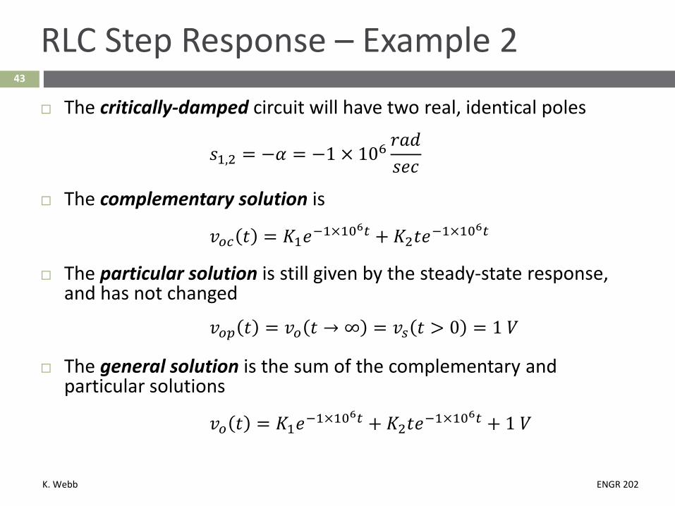
The critically-damped circuit will have two real, identical poles

𝑠𝑠1,2 = −𝛼𝛼 = −1 × 106𝑟𝑟𝑟𝑟𝑑𝑑𝑠𝑠𝑒𝑒𝑠𝑠

The complementary solution is

𝑣𝑣𝑜𝑜𝑜𝑜 𝑡𝑡 = 𝐾𝐾1𝑒𝑒−1×106𝑑𝑑 + 𝐾𝐾2𝑡𝑡𝑒𝑒−1×106𝑑𝑑

The particular solution is still given by the steady-state response, and has not changed

𝑣𝑣𝑜𝑜𝑜𝑜 𝑡𝑡 = 𝑣𝑣𝑜𝑜 𝑡𝑡 → ∞ = 𝑣𝑣𝑠𝑠 𝑡𝑡 > 0 = 1 𝑉𝑉

The general solution is the sum of the complementary and particular solutions

𝑣𝑣𝑜𝑜 𝑡𝑡 = 𝐾𝐾1𝑒𝑒−1×106𝑑𝑑 + 𝐾𝐾2𝑡𝑡𝑒𝑒−1×106𝑑𝑑 + 1 𝑉𝑉

K. Webb ENGR 202

44

RLC Step Response – Example 2

𝑣𝑣𝑜𝑜 𝑡𝑡 = 𝐾𝐾1𝑒𝑒−1×106𝑑𝑑 + 𝐾𝐾2𝑡𝑡𝑒𝑒−1×106𝑑𝑑 + 1 𝑉𝑉

Next, determine the unknown coefficients by applying initial conditions Following the same reasoning as in the previous example, initial conditions are

the same𝑣𝑣𝑜𝑜 0 = 0 and �̇�𝑣𝑜𝑜 0 = 0

Applying the first initial condition𝑣𝑣𝑜𝑜 0 = 𝐾𝐾1 + 1 𝑉𝑉 = 0 → 𝐾𝐾1 = −1 𝑉𝑉

Applying the second initial condition�̇�𝑣𝑜𝑜 𝑡𝑡 = 𝐾𝐾1𝑠𝑠1,2𝑒𝑒𝑠𝑠1,2𝑑𝑑 + 𝐾𝐾2 𝑡𝑡𝑠𝑠1,2𝑒𝑒𝑠𝑠1,2𝑑𝑑 + 𝑒𝑒𝑠𝑠1,2𝑑𝑑

�̇�𝑣𝑜𝑜 0 = 𝐾𝐾1𝑠𝑠1,2 + 𝐾𝐾2 = 0 → 𝐾𝐾2 = −𝑠𝑠1,2𝐾𝐾1 = −1 × 106 𝑉𝑉

The step response of this critically-damped circuit:

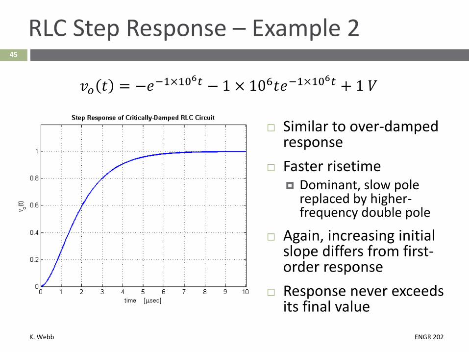
𝑣𝑣𝑜𝑜 𝑡𝑡 = −𝑒𝑒−1×106𝑑𝑑 − 1 × 106𝑡𝑡𝑒𝑒−1×106𝑑𝑑 + 1 𝑉𝑉

K. Webb ENGR 202

45

RLC Step Response – Example 2

Similar to over-damped response

Faster risetime Dominant, slow pole

replaced by higher-frequency double pole

Again, increasing initial slope differs from first-order response

Response never exceeds its final value

𝑣𝑣𝑜𝑜 𝑡𝑡 = −𝑒𝑒−1×106𝑑𝑑 − 1 × 106𝑡𝑡𝑒𝑒−1×106𝑑𝑑 + 1 𝑉𝑉

K. Webb ENGR 202

Under-Damped Circuit Response46

K. Webb ENGR 202

47

RLC Step Response – Example 3

Again decrease the resistance First, determine the damping ratio, 𝜁𝜁

𝜁𝜁 =𝛼𝛼𝜔𝜔0

where, now

𝛼𝛼 =𝑅𝑅2𝐿𝐿

=10 Ω

2 ⋅ 10 𝜇𝜇𝜇𝜇= 500 × 103

𝑟𝑟𝑟𝑟𝑑𝑑𝑠𝑠𝑒𝑒𝑠𝑠

and

𝜔𝜔0 =1𝐿𝐿𝐶𝐶

=1

10 𝜇𝜇𝜇𝜇 ⋅ 100 𝑛𝑛𝑛𝑛= 1 × 106

𝑟𝑟𝑟𝑟𝑑𝑑𝑠𝑠𝑒𝑒𝑠𝑠

The damping ratio is 𝜁𝜁 = 0.5, and the circuit is under-damped The complementary solution will be of the following form:

𝑣𝑣𝑜𝑜𝑜𝑜 𝑡𝑡 = 𝐾𝐾1𝑒𝑒−𝛼𝛼𝑑𝑑 cos 𝜔𝜔𝑑𝑑𝑡𝑡 + 𝐾𝐾2𝑒𝑒−𝛼𝛼𝑑𝑑 sin 𝜔𝜔𝑑𝑑𝑡𝑡

K. Webb ENGR 202

48

RLC Step Response – Example 3

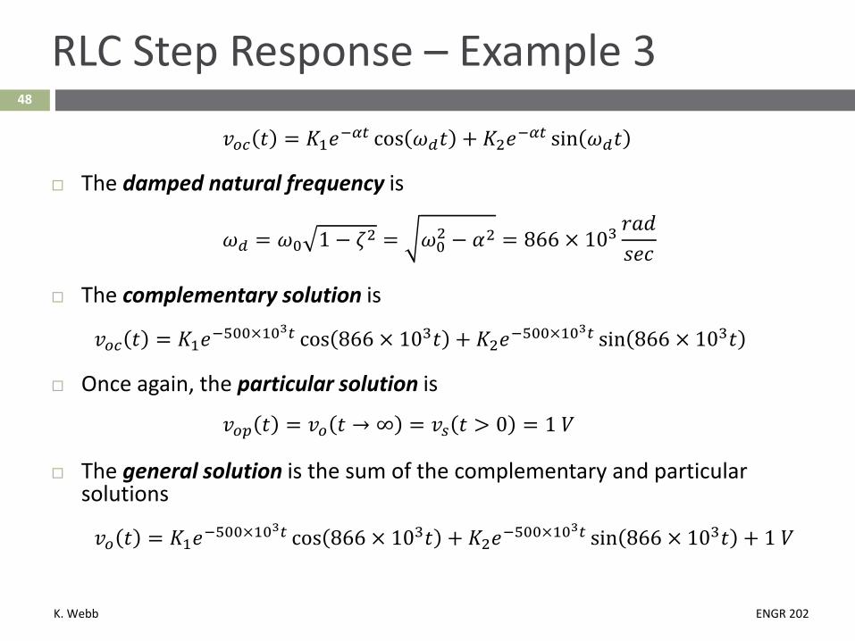
𝑣𝑣𝑜𝑜𝑜𝑜 𝑡𝑡 = 𝐾𝐾1𝑒𝑒−𝛼𝛼𝑑𝑑 cos 𝜔𝜔𝑑𝑑𝑡𝑡 + 𝐾𝐾2𝑒𝑒−𝛼𝛼𝑑𝑑 sin 𝜔𝜔𝑑𝑑𝑡𝑡

The damped natural frequency is

𝜔𝜔𝑑𝑑 = 𝜔𝜔0 1 − 𝜁𝜁2 = 𝜔𝜔02 − 𝛼𝛼2 = 866 × 103𝑟𝑟𝑟𝑟𝑑𝑑𝑠𝑠𝑒𝑒𝑠𝑠

The complementary solution is

𝑣𝑣𝑜𝑜𝑜𝑜 𝑡𝑡 = 𝐾𝐾1𝑒𝑒−500×103𝑑𝑑 cos 866 × 103𝑡𝑡 + 𝐾𝐾2𝑒𝑒−500×103𝑑𝑑 sin 866 × 103𝑡𝑡

Once again, the particular solution is

𝑣𝑣𝑜𝑜𝑜𝑜 𝑡𝑡 = 𝑣𝑣𝑜𝑜 𝑡𝑡 → ∞ = 𝑣𝑣𝑠𝑠 𝑡𝑡 > 0 = 1 𝑉𝑉

The general solution is the sum of the complementary and particular solutions

𝑣𝑣𝑜𝑜 𝑡𝑡 = 𝐾𝐾1𝑒𝑒−500×103𝑑𝑑 cos 866 × 103𝑡𝑡 + 𝐾𝐾2𝑒𝑒−500×103𝑑𝑑 sin 866 × 103𝑡𝑡 + 1 𝑉𝑉

K. Webb ENGR 202

49

RLC Step Response – Example 3

𝑣𝑣𝑜𝑜 𝑡𝑡 = 𝐾𝐾1𝑒𝑒−𝛼𝛼𝑑𝑑 cos 𝜔𝜔𝑑𝑑𝑡𝑡 + 𝐾𝐾2𝑒𝑒−𝛼𝛼𝑑𝑑 sin 𝜔𝜔𝑑𝑑𝑡𝑡 + 1 𝑉𝑉

Next, determine the unknown coefficients by applying initial conditions𝑣𝑣𝑜𝑜 0 = 0 and �̇�𝑣𝑜𝑜 0 = 0

Applying the first initial condition

𝑣𝑣𝑜𝑜 0 = 𝐾𝐾1 + 1 𝑉𝑉 = 0𝐾𝐾1 = −1 𝑉𝑉

Applying the second initial condition

�̇�𝑣𝑜𝑜 𝑡𝑡 = 𝐾𝐾1 −𝜔𝜔𝑑𝑑𝑒𝑒−𝛼𝛼𝑑𝑑 sin 𝜔𝜔𝑑𝑑𝑡𝑡 − 𝛼𝛼𝑒𝑒−𝛼𝛼𝑑𝑑 cos 𝜔𝜔𝑑𝑑𝑡𝑡

+𝐾𝐾2 𝜔𝜔𝑑𝑑𝑒𝑒−𝛼𝛼𝑑𝑑 cos 𝜔𝜔𝑑𝑑𝑡𝑡 − 𝛼𝛼𝑒𝑒−𝛼𝛼𝑑𝑑 sin 𝜔𝜔𝑑𝑑𝑡𝑡

�̇�𝑣𝑜𝑜 0 = −𝐾𝐾1𝛼𝛼 + 𝐾𝐾2𝜔𝜔𝑑𝑑 = 0

𝐾𝐾2 = 𝐾𝐾1𝛼𝛼𝜔𝜔𝑑𝑑

= −500 × 103

866 × 103 = −0.58

K. Webb ENGR 202

50

RLC Step Response – Example 3

The step response for this under-damped RLC circuit is

𝑣𝑣𝑜𝑜 𝑡𝑡 = −𝑒𝑒−500×103𝑑𝑑 cos 866 × 103𝑡𝑡

−0.58𝑒𝑒−500×103𝑑𝑑 sin 866 × 103𝑡𝑡 + 1 𝑉𝑉

Damped oscillatory components Overshoot Possible ringing

Exponential damping Oscillatory components decay to zero Rate of decay determined by 𝛼𝛼, real part of poles

K. Webb ENGR 202

51

RLC Step Response – Example 3

Overshoot Response exceeds its

final value

Ringing Response oscillate

about its final value Not much ringing in

this example

Damping ratio Overshoot and ringing

are inversely proportional to 𝜁𝜁

K. Webb ENGR 202

Step Response Characteristics52

K. Webb ENGR 202

53

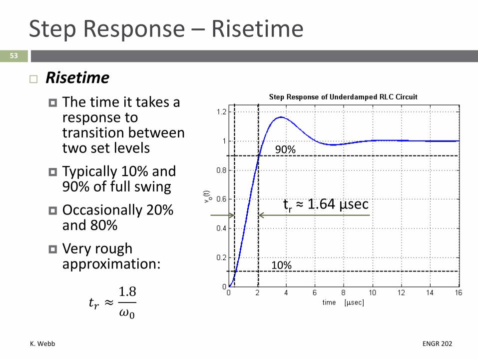
Step Response – Risetime

Risetime The time it takes a

response to transition between two set levels

Typically 10% and 90% of full swing

Occasionally 20% and 80%

Very rough approximation:

𝑡𝑡𝑟𝑟 ≈1.8𝜔𝜔0

90%

10%

tr ≈ 1.64 μsec

K. Webb ENGR 202

54

Step Response – Overshoot

Overshoot Response’s excursion

beyond its final value Expressed as a

percentage of the full-scale swing

Inversely proportional to damping ratio

%OS ≈ 16%

ζ %OS

0.45 20

0.5 16

0.6 10

0.7 5

%𝑂𝑂𝑂𝑂 = 𝑒𝑒− 𝜁𝜁𝜁𝜁

1−𝜁𝜁2 ⋅ 100%

K. Webb ENGR 202

55

Step Response – Settling Time

Settling time The time it takes a

response to settle (finally) to within some percentage of the final value

Typically ±1%, ±2%, or ± 5%

Inversely proportional to the real part of the circuit’s poles (roots of the characteristic equation)

For ±1% settling time:

𝑡𝑡𝑠𝑠 ≈4.6𝛼𝛼 =

4.6𝜁𝜁𝜔𝜔0

+1%

-1%

𝑡𝑡𝑠𝑠 = 8.8 𝜇𝜇𝑠𝑠𝑒𝑒𝑠𝑠

K. Webb ENGR 202

Example Problems56

K. Webb ENGR 202

Determine: R and L, such that

𝑂𝑂. 𝑂𝑂. = 10% 𝑡𝑡𝑠𝑠 ≈ 2𝜇𝜇𝑠𝑠𝑒𝑒𝑠𝑠

System poles 𝑣𝑣𝑜𝑜 𝑡𝑡 for 𝑡𝑡 ≥ 0

K. Webb ENGR 202

K. Webb ENGR 202

K. Webb ENGR 202

K. Webb ENGR 202

K. Webb ENGR 202

K. Webb ENGR 202

Determine the minimum resistance for 0% overshoot.