MIT 9.17: Systems Neuroscience Laboratory    

 

Section 2. Practical Skills    

2.1 Anatomical Terminology    

2.2 Concepts and Equipment in Neurophysiology    

2.3 Practical Lab      

Overview  

This section will introduce you to the skills and knowledge necessary in neuroscience: anatomical termi- nology, the fundamentals of electrical signals, how to setup use basic signal processing equipment, and how to use stereotaxic equipment. It is vitally important that you learn this section well, as you will continue to utilize this equipment for the rest of the semester.

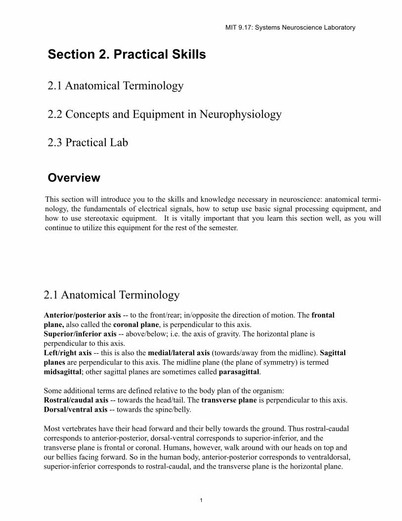
               2.1 Anatomical Terminology  Anterior/posterior axis -- to the front/rear; in/opposite the direction of motion. The frontal plane, also called the coronal plane, is perpendicular to this axis. Superior/inferior axis -- above/below; i.e. the axis of gravity. The horizontal plane is perpendicular to this axis. Left/right axis -- this is also the medial/lateral axis (towards/away from the midline). Sagittal planes are perpendicular to this axis. The midline plane (the plane of symmetry) is termed midsagittal; other sagittal planes are sometimes called parasagittal.  Some additional terms are defined relative to the body plan of the organism: Rostral/caudal axis -- towards the head/tail. The transverse plane is perpendicular to this axis. Dorsal/ventral axis -- towards the spine/belly.

 

 Most vertebrates have their head forward and their belly towards the ground. Thus rostral-caudal corresponds to anterior-posterior, dorsal-ventral corresponds to superior-inferior, and the transverse plane is frontal or coronal. Humans, however, walk around with our heads on top and our bellies facing forward. So in the human body, anterior-posterior corresponds to ventraldorsal, superior-inferior corresponds to rostral-caudal, and the transverse plane is the horizontal plane.

1

���The human nervous system makes a fairly sharp bend in the hindbrain and midbrain, however, so most of the brain is oriented similarly to other organisms; thus in the brain, rostral can mean “towards the forehead”, or anterior, and dorsal can mean “towards the scalp”, or superior �Superficial/deep -- nearer/further from the surface (e.g. layers of cortex).

�Proximal/distal -- nearer/further from the body, for an appendage. Likewise parts of the dendritic tree may be termed proximal or distal.

�

�Ispilateral/contralateral -- same/opposite side.

�

DorsalCaudal

Ventral

Rostral

Rostral

Frontalor

transverse

DorsalHorizontal section

Ventral

Caudal

Sagittal section

SuperiorPosterior

MedialLateral

Anterior

Transverseplane

Midsagittalplane

Inferior

Frontalplane

Anterior Posterior

Sagittal

Horizontal

Frontal (transverse)

Coronal Plane

Horizontal Plane

Sagittal Plane

Image by MIT OpenCourseWare.

Image by MIT OpenCourseWare.

  MIT 9.17: Systems Neuroscience Laboratory    2.2 Concepts and Equipment in Neurophysiology

   Basic concepts you should be familiar with from physics:

   Charge (Q)

The fundamental charged particles are electrons and protons. The unit of charge is the Coulomb. In neurobiology, charge is mostly carried by ions in solution: Na+, K+ and Ca2+ cations and the Cl- anion are the most important. Electrons are the charge carriers in wires and electrodes.

 

 Voltage (V)

The voltage between two points is the amount of work done when a unit charge is moved from one point to the other. Equivalently, it is the difference in potential energy of a unit charge at the two locations. The unit of voltage is the Volt: 1 volt = 1 joule / coulomb. In neurobiology, we are often interested in the membrane potential, the voltage difference between the inside and outside of a cell. We won’t be measuring membrane potentials (“intracellular recording”) in this course. Instead, we will be measuring the voltage in the extracellular space (“extracellular recording”, also called a “field potential”) relative to a distant reference electrode -- see below.

   Current (I)

Current is the amount of charge moving past a fixed point per unit time. The unit of current is the Ampere: 1 amp = 1 coulomb / second.

   Resistance (R)

If a potential difference (Voltage) is applied to the two ends of a conductor, current will flow. Resistance is defined as the potential difference divided by the current (R = V / I). Resistance is a property of the conductor and characterizes how much the conductor “resists” the flow of charge. It is different for different materials. The unit of resistance is the Ohm. 1 ohm = 1 volt / amp. Conductance (G) is the inverse of resistance (G = 1 / R).

 

 Ohm’s Law

For many materials, including metallic conductors and ions in solution, the resistance is the same regardless of the voltage that we use. This important relationship is known as Ohm’s Law.

 

 V = I * R or I = V / R = V * G, in terms of conductance.

 The analogy most commonly given is to water in a pipe. Charge corresponds to the water. The current is the flow rate past a particular point (gallons/sec). The voltage is the pressure difference between the two ends of the pipe, driving the flow. And the resistance reflects the narrowness of the pipe, friction between the fluid and walls, etc.  Capacitance (C)

If there is no conductive path connecting two points that have a voltage potential between them (e.g. a potential difference applied to two metal plates in air), charge will accumulate at the two points. If 1 volt potential between two plates causes an accumulation of 1 coulomb of charge (i.e. 1 coulomb of  

3

  MIT 9.17: Systems Neuroscience Laboratory    positive charge on one plate and one coulomb of negative charge on the other), the capacitance is defined as 1 Farad (1 farad = 1 coulomb / volt). Think of capacitance as the ability of (e.g. two plates) to store charge.

 

 In general, the capacitance is proportional to the area of the two plates, inversely proportional to their separation, and depends on the material occupying that separation. In neurobiology, the “plates” are the conducting aqueous solutions inside and outside the cell, and the non-conducting separator is the cell membrane. Cell membranes have approximately constant thickness and composition, so a cell’s capacitance is approximately proportional to its surface area, ~1 uF / cm2. The exception is myelinated axons, where the extra wrappings of membrane increase the separation between conducting “plates” and thus decrease capacitance.

 

     Voltage “signals”

 As you know, neurons communicate through neurotransmitters released in response to changes in membrane potential. A change in membrane potential (e.g. action potentials) is the fundamental way in which information is transmitted along nerve fibers. As a result, the measurement of potentials within and around neurons turns out to be a very useful tool for assessing information processing in the nervous system. Much of this course is devoted to measuring such potentials, understanding where they come from, and understanding what they can tell us about the processing and transmission of information in the nervous system (i.e. “electrophysiology”).

 

 Given the importance of voltage potentials, it is critical that you understand what a voltage potential is (see above), and how we measure it. Remember that a potential is always defined between two points. In electrophysiology, the potential at a location of interest is typically determined relative to some distant reference electrode, and the preparation is “grounded” (an electrical path to the Earth is provided). We then talk about “the potential at location X”, with the understanding that we mean “relative to the grounded animal”. This works because animal tissue is mostly saltwater, a good conductor -- all distant locations are thus at approximately equal potential, assuming no potentials are being generated local to the reference electrode. (Side note: For intracellular recording, the potential relative to the immediate extracellular space may be of greater theoretical interest, as this is the voltage experienced by voltage-sensitive channels within the membrane; however, this is more difficult to obtain, and often unnecessary. Voltage differences in the extracellular space are typically much smaller than changes in the membrane potential, tens or hundreds of microvolts vs. a few or tens of millivolts. Thus, a distant reference provides a decent approximation to the true “transmembrane potential”.)

 We have mentioned that we will be recording extracellular potentials in this course. What is the source of these? More will be said about this in lecture, but the short answer is: extracellular potentials reflect transmembrane currents in the vicinity of the electrode tip, rather than the membrane potential of nearby neuronal elements. In general, inward currents (e.g. Na+ ions flowing into a cell or axon during the rising phase of an action potential) will produce a negative potential in the extracellular space, and outward currents will produce a positive potential. The

 

4

  MIT 9.17: Systems Neuroscience Laboratory    

amplitude of these potentials depends strongly on the localization of the underlying currents, the positioning of the electrode tip relative to the membranes experiencing the currents, and even the geometry and membrane properties of the cellular elements. Fortunately, we don’t usually need many of these details to produce useful recordings of action potentials. This is because action potentials feature such high current densities, and such stereotyped timecourses, that they are easy to identify in the extracellular potential. And because the action potential is such a stereotyped all-or- nothing event, we are typically more interested in the number and times at which they occur rather than the details of the underlying currents.

 

 Typically, the voltage potential will be accessed with a recording electrode (a good conductor, insulated except at the very tip), amplified and then carried on a conductor (i.e. wire) to a display or recording device. A typical wire is a BNC cable. It has an inner conductive core, and an outer conductive “shield”. The recording equipment we will use in this course will be hooked up so that the potentials we are interested in should be measured between the BNC inner core conductor and the outer shield conductor (“ground”).

 

 One goal of the lab sessions is to teach you a common way in which these potentials are observed and measured – using an oscilloscope. A document describing the oscilloscope is also available on the course web site. If you do not understand the use of your oscilloscope, please ask one of your instructors or TAs for a brief tutorial.

 

   Time

   

The voltages we are recording are not constant (that would not be very interesting!). Indeed, they can change very rapidly. We often refer to the voltage measured across time as the “voltage signal” or the “voltage waveform.”

 

 Side bar: What does the time course of an action potential look like (draw one)? What is the relevant time scale to describe a single action potential (i.e. put a scale on the x axis)? (hours, minutes, seconds, milliseconds, microseconds?)

 

 When working with voltage signals that vary with time, one of the fundamental concepts is that any such signal can be thought of not just as a voltage signal that varies with time, but as the sum of many infinitely long sinusoids of different frequencies and phases (time shifts relative to each other). These two ways of describing the voltage waveform are EXACTLY equivalent. The sinusoidal format is called the Fourier representation of the voltage signal. The Fourier representation has useful properties and advantages over the time-based representation. We will talk more about this as the course goes on. For now, you should minimally understand that sinusoids are an important type of voltage signal.

 

5

  MIT 9.17: Systems Neuroscience Laboratory    Here are some basic concepts you should know about sinusoids and other “periodic” signals:

   Frequency and Period

 

 The frequency of a sinusoidal waveform is simply the number of times it moves up and down in one second. (Actually, we only count the “ups” or the “downs”, but not both). The unit of frequency is Hertz (cycles / second). A sinusoid that moves up once per second is said to have a frequency of 1 Hz. A sinusoid that moves up twice per second is said to have a frequency of 2 Hz.

   

Side note: Given your drawing of a single action potential above, what is the approximate “fundamental” (i.e. dominant) frequency of an action potential? (hint: think of the entire action potential as one cycle of an infinitely long sinusoid).

 

 Side note: Computers now have clock frequencies of over 1 gigahertz. How many cycles per second does a 1 gigahertz sinusoid undergo? Compare the fundamental frequency of a computer clock and an action potential.

 

 Closely related to frequency is the concept of “period.” The period of a sinusoidal signal is the time between each of the “ups” (or, equivalently, each of the “downs”). Period is thus the inverse of frequency: (frequency (Hz) = 1 / period (sec) ). For example, a sinusoid that moves up every 1 sec has a period of 1 sec (and a frequency of: 1 cycle / 1 sec = 1 Hz). A sinusoid that moves up every 0.1 sec (100 msec) has a period of 100 msec (and a frequency of: 1 cycle / 0.1 sec = 10 Hz).

   

Side note: What is the period at which the earth rotates around its axis? What is the frequency?      

 Amplitude

 Amplitude is simply the magnitude of the voltage signal (i.e. units of volts). Because the signal varies with time, we often refer to the “peak amplitude” (e.g. 200 mVolts). Sinusoidal amplitudes are, by convention, often measured as the “peak-to-peak” amplitude. This is defined as the difference between the highest point (“up”) and the lowest point (“down”) of the sinusoid. The units are still in volts (or millivolts, etc.).

 

6

  MIT 9.17: Systems Neuroscience Laboratory      

2.3 Practical Laboratory Skills  This lab is intended to familiarize you with some of the equipment that we will be using throughout the course. The lab is divided into three sections: Anatomy, Physiology 1 and Physiology 2. We will direct your group to the correct station at each time.  Anatomy

 

 Your station will include a microscope, two sets of slides, a rat brain atlas and a stereotaxic apparatus. Each set of slides shows an electrode track with a small lesion at the location of the electrode tip, such as you would generate at the end of a physiology experiment to verify the location from which you recorded. The goal of this lab is to identify the recording locations from the slides with the help of the atlas, then use the stereotax to position an electrode at those locations in a clay “rat brain”.  Determine the electrode trajectory and recording location 1) Examine the first set of slides under low power. What is the plane of section? 2) Use the atlas to determine the starting and ending coordinates of the series. Note which structures or anatomical landmarks were useful to you in making this determination. 3) Determine the stereotaxic coordinates of the center of the lesion: rostral-caudal relative to bregma, lateral to the midline, and depth from the surface of the brain. 4) If the electrode traveled at an angle, also determine the coordinates where it entered the brain, the angle at which it traveled, and the distance that it traveled from the surface of the brain. 5) Also describe the recording location in anatomical terms e.g. the ventrolateral portion of the nucleus, or layer of area of neocortex.  Use the stereotax to position an electrode 1) A clay “rat head” should already be positioned in the stereotax. If this were a real rat, the skull would be immobilized by the ear bars and bite plate. Check that the top of the “skull” is level; ask a TA to help you adjust it if you don’t think that it is. 2) Identify the sutures on the top of the skull (junctions between the plates of the skull). There should be a midline suture and two crossing sutures. The more anterior intersection is the point called “bregma”; this is the most common reference point for rostal-caudal positioning. The posterior intersection is called “lambda”; it is sometimes used for positioning at more caudal sites.

 

7

  MIT 9.17: Systems Neuroscience Laboratory      

Photograph of a dorsal surface of a rat skull removed due to copyright restrictions. See Cooley, R. K.,and C. H. Vanderwolf. Stereotaxic Surgery in the Rat: A Photographic Series. A. J. Kirby Co., 2005.

The dorsal surface of the rat skull. Anterior is to the right.

 

 3) Our stereotaxes are not equipped for precise measurements in the rostral-caudal dimension. Measure this dimension along the midline with a ruler and mark it lightly on the clay. You should be able to achieve a precision of about a quarter millimeter; the location of bregma has about this much uncertainty anyway due to the irregular nature of the sutures. 4) Place an electrode in the stereotax arm. The arm should be directly vertical, not angled, and the electrode should also be aligned vertically. 5) Adjust the electrode position until the tip is just above the mark you’ve made on the midline to indicate the rostral-caudal coordinate. Look at it both from directly behind and from the side to make sure it is correctly positioned. Double-check that it is still vertical. 6) Retract the electrode a bit, then move it laterally the correct distance to the position where the electrode entered the brain. Lower it until the tip just touches the surface. 7) If the electrode is to travel at an angle, make a small mark on the clay with the electrode tip, then retract it. Adjust the angle, then reposition the electrode tip where it should enter the clay. 8) Advance the electrode the correct distance to the recording site. 9) Have a TA check that your electrode appears to be correctly positioned.

 

 Repeat these steps for the second series of slides, allowing a different member of your group to make the various measurements, etc.

 

8

  MIT 9.17: Systems Neuroscience Laboratory      Physiology 1

 

 Your station will include a waveform generator, oscilloscope, amplifier/filters and associated cables. You will measure voltage waveforms using the oscilloscope, investigate the gain and range of the amplifier, and deter- mine the effect of the filter settings on sinusoidal signals of different frequencies.  Oscilloscope basics 1) Connect power cables for the waveform generator and oscilloscope and turn them on. Connect the output of the waveform generator to the input (CH1) of the oscilloscope. 2) Set the waveform generator to generate a sine wave with an amplitude of 2 V and a frequency of 500 Hz. Adjust the vertical (amplitude) and horizontal (time-base) scales of the oscilloscope until you have a clear view of the signal. What amplitude does the oscilloscope indicate? Note that there are different ways to measure amplitude: peak-to-peak is often used to describe the noise level; baseline-to-peak makes sense when signals are described by functions e.g. f(t) = A*sin(ω*t+θ) is a sinusoid with baseline-to-peak amplitude A; you may even see Vrms (“root mean-squared”), a measure of amplitude that is related to a signal’s power. Always be clear about how you are measuring “amplitude”. Which definition does the waveform generator use when putting out a “2 V” sinusoid? 3) The oscilloscope may be triggered, in which case it will display data centered on the time of the triggering event. Press the trigger menu button, and set the scope to trigger off CH1, edge, rising, normal mode. Now you can use the right-most knob to adjust the level that will cause the scope to trigger, so that the waveform appears consistently at the same location. This makes it easy to measure the period and compute the frequency. How does it compare with the setting of the waveform generator? 4) Experiment with several different waveforms, amplitudes and frequencies. Each time you should adjust the scope settings to obtain a good view, measure the amplitude and period with the scope, and compare them to the waveform generator settings. Explore the limits of amplitude and frequency at which you can still obtain and measure a good waveform.  Amplifier and filter basics 1) Split the output of the waveform generator with a BNC “T-junction”. Send the signal directly to CH1, and also to the inputs of the amplifier. Connect the amplifier output to CH2. 2) Generate a 500 Hz, 20 mV sinusoid. Set the high-pass filter at 30 Hz, the low-pass filter at 3 kHz, and the gain at 100. Adjust the scope settings to obtain a good view (vertical scale can be set separately for the two channels). Change the amplifier gain to 1000 and readjust the scope. Change the amplifier gain to 10,000 and readjust the scope. What has happened and why? 3) Set the amplifier gain to 100, and the filters at 30 Hz and 300 Hz. Generate 20 mV sine waves at the follow- ing frequencies and measure the amplitude of the signal after amplification and filtering: 10 Hz, 20 Hz, 30 Hz, 50 Hz, 100 Hz, 200 Hz, 300 Hz, 500 Hz, 1 kHz, 2 kHz, 3 kHz, 5 kHz, 10 kHz. Plot the amplitude against the logarithm of the frequency.

 

9

  MIT 9.17: Systems Neuroscience Laboratory      4) Set the filters to 300 Hz and 3 kHz (typical settings for isolating action potentials) and repeat step #3.

 

 Physiology 2

 

 This section will expand on Physiology 1 by digitizing signals with an analog-to-digital (A/D) converter and computing the power spectra to visualize them in the frequency domain. In addition, we will explore some of the sources of noise that commonly plague electrophysiologists.

 

 A/D conversion and power spectra 1) Connect the waveform generator to the amplifier, then split the signal and send it to both the oscilloscope and channel 1 of the A/D converter. Connect the A/D converter to the computer. Open the Chart program. Go to the Settings >> Channels menu and review the settings for channel 1, in particular the input range (+/- 10 V) and sampling frequency (10 kHz). 2) Set the waveform generator to output a 20 mV sine wave at 500 Hz. Set the amplifier gain to 100 and the filters to 3 Hz and 10 kHz. Verify the signal reaching the oscilloscope. Click the Run button in Chart’s data window, and it will begin collecting data. Click the Stop button. You can expand or contract the range of data displayed with the controls to the left of and below the data chart. 3) Select a segment of data by clicking and dragging, then go to the Windows menu and select Spectrum. A new window should appear with a power spectrum of the selected data. At what frequency does the peak occur? You can select a new segment of data, and the spectrum will be computed and displayed automati- cally (you don’t have to go through the Windows menu each time). You can save a screenshot of the spec- trum window by pressing Command-Shift-4, then spacebar, then clicking in the window; this creates a file on the desktop which can be opened for viewing by double-clicking. 4) Try varying the amplitude or frequency of the signal and observing the changes in the power spectrum. Try different waveforms (triangle wave, square wave, short pulses, etc). The peaks you see at multiples of the base frequency are called “harmonics”; they occur with signals that are periodic but non-sinusoidal. 5) Set the waveform generator to output “noise”. What does it look like on the scope? What does the spec- trum look like? Take a few spectra – the value at any particular frequency is highly random on each trial, but you can still describe the overall shape of the spectrum. Now try varying the filter settings on your amplifier, for example to the ranges used in Physiology 1. How do the resulting noise spectra compare to the plots of amplitude vs. log(frequency) you created?  Electrodes and noise There will be a beaker of saline with a couple of electrodes in it. You can use either the oscilloscope or the Chart program, or both, for this portion of the lab. 1) Connect the two stainless steel pins to the inputs of the amplifier. What type of signal do you see? What is its frequency? This is radiative noise. The power lines in the wall carry alternating current at 60 Hz (in this country, 50 Hz in some others). Power cords and other sources thus emit electromagnetic fields at that frequency. Set up the Farraday cage around your beaker and amplifier, and ground it. This should reduce the 60 Hz, although possibly not eliminate it. Make sure that power cords do not run though the cage; in fact it’s often helpful to plug things in at the other end of the lab bench. Try reaching in to the Farraday cage, both while touching ground and while ungrounded. You can act as an antenna, bringing 60 Hz noise into the shielded space. The amplifier also has a line filter. This is a narrow band-reject filter that allows frequencies less than or greater than 60 Hz to pass without attenuation, while blocking a narrow range of frequencies right around 60 Hz.

 

10

  MIT 9.17: Systems Neuroscience Laboratory  

   2) Connect the tungsten electrode to input 1 of the amplifier. Your noise problems will increase dramati- cally. The tungsten electrode has a high impedance (like resistance for time-varying signals), causing any current fluctuation to result in large voltages (remember Ohm’s Law). From here, the lab becomes more trial-and-error as you try to minimize noise sources.  Some types of noise that you might see: -- Low-frequency drift, and sensitivity to low-frequency fields e.g. as you wave your arm near the electrode. -- 60 Hz, again, and harder to eliminate completely. -- Harmonics of 60 Hz. These are best detected with the spectrum, although if they’re strong you might identify them on the scope. -- Higher-freqency signals due to the screens on the oscilloscope or monitor. -- Vibrations e.g. when you thump the bench-top with your hand

 

 Some things that you might try: -- Connect the Common input of the amplifier to the Farraday cage, or to the reference electrode, or to a separate grounding electrode. -- Use a Ag/AgCl wire as the reference and/or the grounding electrode. -- Shorten the wiring length between the electrodes and the amplifier input as much as possible (no extra alligator clips). -- Use aluminum foil for extra shielding. -- Place bubble wrap under the beaker/electrodes to dampen any vibrations.

 

11

MIT OpenCourseWarehttp://ocw.mit.edu

9.17 Systems Neuroscience LabSpring 2013

For information about citing these materials or our Terms of Use, visit: http://ocw.mit.edu/terms.