Section 2

Generic Equipment and Devices

EPA/452/B-02-001

1-1

Chapter 1

Hoods, Ductwork and Stacks

William M. VatavukInnovative Strategies and Economics GroupAir Quality Strategies and Standards DivisionOffice of Air Quality Planning and StandardsU.S. Environmental Protection AgencyResearch Triangle Park, NC 27711

December 1995

EPA/452/B-02-001

1-2

Contents

1.1 Introduction .................................................................................................................................... 1-3

1.2 Equipment Description ................................................................................................................... 1-3

1.2.1 Hoods ................................................................................................................................. 1-41.2.1.1 Types of Hoods ................................................................................................... 1-4

1.2.2 Ductwork ............................................................................................................................ 1-61.2.2.1 Ductwork Components ........................................................................................ 1-8

1.2.3 Stacks ............................................................................................................................... 1-12

1.3 Design Procedures ........................................................................................................................ 1-13

1.3.1 Design Fundamentals ...................................................................................................... 1-131.3.1.1 The Bernoulli Equation ....................................................................................... 1-131.3.1.2 Pressure: Static, Velocity, and Total ................................................................... 1-171.3.1.3 Temperature and Pressure Adjustments ............................................................. 1-20

1.3.2 Hood Design Procedure ................................................................................................... 1-211.3.2.1 Hood Design Factors .......................................................................................... 1-211.3.2.2 Hood Sizing Procedure ....................................................................................... 1-261.3.3 Ductwork Design Procedure ................................................................................. 1-281.3.3.1 Two Ductwork Design Approaches ................................................................... 1-281.3.3.2 Ductwork Design Parameters .............................................................................. 1-281.3.3.3 Ductwork Pressure Drop .................................................................................... 1-31

1.3.4 Stack Design Procedures ................................................................................................. 1-351.3.4.1 Calculating Stack Diameter ................................................................................. 1-361.3.4.2 Calculating Stack Height .................................................................................... 1-371.3.4.3 Calculating Stack Draft ....................................................................................... 1-38

1.4 Estimating Total Capital Investment .............................................................................................. 1-40

1.4.1 Equipment Costs .............................................................................................................. 1-401.4.1.1 Hood Costs ......................................................................................................... 1-401.4.1.2 Ductwork Costs .................................................................................................. 1-411.4.1.3 Stack Costs ......................................................................................................... 1-46

1.4.2 Taxes, Freight, and Instrumentation Costs ....................................................................... 1-59

1.4.3 Purchased Equipment Cost .............................................................................................. 1-50

1.4.4 Installation Costs ............................................................................................................. 1-50

1.5 Estimating Total Annual Cost ........................................................................................................ 1-51

1.5.1 Direct Annual Costs ......................................................................................................... 1-51

1.5.2 Indirect Annual Costs ...................................................................................................... 1-52

1.5.3 Total Annual Cost ............................................................................................................ 1-51

1.6 Acknowledgements ....................................................................................................................... 1-55

1-3

1.1 Introduction

Most control devices are located some distance from the emission sources they control.This separation may be needed for several reasons. For one thing, there may not be enough roomto install the control device close to the source. Or, the device may collect emissions from severalsources located throughout the facility and, hence, must be sited at some convenient, equidistantlocation. Or, it may be that required utility connections for the control device are only available atsome remote site. Regardless of the reason, the waste gas stream must be conveyed from thesource to the control device and from there to a stack before it can be released to the atmosphere.

The type of equipment needed to convey the waste gas are the same for most kinds ofcontrol devices. These are: (1) hoods, (2) ductwork, (3) stacks, and (4) fans. Together, theseitems comprise a ventilation system. A hood is used to capture the emissions at the source; ductwork,to convey them to the control device; a stack, to disperse them after they leave the device; and afan, to provide the energy for moving them through the control system. This section covers the firstthree kinds of equipment. However, because they constitute such a broad and complex subject,fans will be dealt with in a another section of this Manual to be developed in the future. Only shortstacks (100-120 feet high or less) are covered. Typically, short stacks are included with packagedcontrol systems or added to them. So-called “tall stacks” (“chimneys”), used at power plants orother sources where the exhaust gases must be dispersed over great distances, will not be discussedin this section.

This section presents all the information one would need to develop study (± 30%-accurate)cost estimates for hoods, ductwork, and stacks. Accordingly, the following sections include: (1)descriptions of the types of equipment used in air pollution control ventilation systems, (2) proceduresfor sizing (designing) this equipment, and (3) methodologies and data for estimating their capitaland annual costs. Throughout the chapter are several illustrations (example problems) that showthe reader how to apply the various sizing and costing methodologies.

1.2 Equipment Description

In this section, the kinds of hoods, ductwork, and stacks used in air pollution controlsystems are described, each in a separate subsection. These descriptions have been based oninformation obtained from standard ventilation and air pollution control references, journal articles,and equipment vendors.

1-4

1.2.1 Hoods

Of the several components of an air pollution control system, the capture device is themost important. This should be self-evident, for if emissions are not efficiently captured at thesource they cannot be conveyed to and removed by a control device. There are two generalcategories of capture devices: (1) direct exhaust connections (DEC) and (2) hoods. As the nameimplies, a DEC is a section of duct (typically an elbow) into which the emissions directly flow.These connections often are used when the emission source is itself a duct or vent, such as aprocess vent in a chemical manufacturing plant or petroleum refinery. (See following discussion on“Ductwork”.)

Hoods comprise a much broader category than DECs. They are used to capture particulates,gases, and/or mists emitted from a variety of sources, such as basic oxygen steelmaking furnaces,welding operations, and electroplating tanks. The hooded processes are generally categorized aseither “hot” or “cold,” a delineation that, in turn, influences hood selection, placement, and design.

The source characteristics also influence the materials from which a hood is fabricated.Mild (carbon) steel is the material of choice for applications where the emission stream is noncorrosiveand of moderate temperature. However, where corrosive substances (e.g., acid gases) are presentin high enough concentrations, stainless steels or plastics (e.g., fiberglass-reinforced plastic, orFRP) are required. As most hoods are custom-designed and built, the vendor involved woulddetermine which material would be optimal for a given application.

1.2.1.1 Types of Hoods

Although the names of certain hoods vary, depending on which ventilation source oneconsults, there is general agreement as to how they are classified. There are four types of hoods:(1) enclosures, (2) booths, (3) captor (capture) hoods, and (4) receptor (receiving) hoods.[1,2]

Enclosures are of two types: (1) those that are completely closed to the outside environmentand (2) those that have openings for material input/output. The first type is only used when handlingradioactive materials, which must be handled by remote manipulators. They are also dust- andgas-tight. These kinds of enclosures are rarely used in air pollution control. The second type, haveapplications in several areas, such as the control of emissions from electric arc furnaces and fromscreening and bin filling operations. They are equipped with small wall openings (natural draftopenings—”NDOs”) that allow for material to be moved in or out and for ventilation. However,the area of these openings must be small compared with the total area of the enclosure walls(typically, 5% or less).

1-5

Another application of total enclosures is in the measurement of the capture efficiency ofvolatile organic compound (VOC) control devices. Capture efficiency is that fraction of all VOCsgenerated at, and released by, an affected facility that is directed to the control device. In thisapplication, a total enclosure is a temporary structure that completely surrounds an emitting processso that all VOC emissions are captured for discharge through ducts or stacks. The air flow throughthe total enclosure must be high enough to keep the concentration of the VOC mixture inside theenclosure within both the Occupational Safety and Health Administration (OSHA) healthrequirement limits and the vapor explosive limits. (The latter are typically set at 25% of the lowerexplosive limit (LEL) for the VOC mixture in question.) In addition, the overall face velocity of airflowing through the enclosure must be at least 200 ft/min.[3]

The surfaces of temporary total enclosures are usually constructed either of plastic film orof such rigid materials as insulation panels or plywood. Plastic film offers the advantages of beinglightweight, transparent, inexpensive, and easy to work with. However, it is flimsy, flammable, andhas a relatively low melting point. In addition, the plastic must be hung on a framework of wood,plastic piping, or scaffolding.

Although rigid materials are more expensive and less workable than plastic, they are moredurable and can withstand larger pressure differentials between the enclosure interior and exterior.Total enclosure design specifications (which have been incorporated into several EPA emissionstandards) are contained in the EPA report, The Measurement Solution: Using a Temporary TotalEnclosure for Capture Testing.[4]

Booths are like enclosures, in that they surround the emission source, except for a wall (orportion thereof) that is omitted to allow access by operators and equipment. Like enclosures,booths must be large enough to prevent particulates from impinging on the inner walls. They areused with such operations (and emission sources) such as spray painting and portable grinding,polishing, and buffing operations.

Captor hoods (also termed active or external hoods) do not enclose the source at all.Consisting of one to three sides, they are located at a short distance from the source and draw theemissions into them via fans. Captor hoods are further classified as side-draft/backdraft, slot,downdraft, and high-velocity, low-volume (HVLV) hoods.

A side-draft/back-draft hood is typically located to the side/behind of an emission source,but as close to it as possible, as air velocities decrease inversely (and sharply) with distance.Examples of these include snorkel-type welding hoods and side shake-out hoods.

A slot hood operates in a manner similar to a side-draft/back-draft. However, the inletopening (face) is much smaller, being long and narrow. Moreover, a slot hood is situated at theperiphery of an emission source, such as a narrow, open tank. This type of hood is also employedwith bench welding operations.

1-6

While slot and side-draft/back-draft hoods are located beside/behind a source, a downdrafthood is situated immediately beneath it. It draws pollutant-laden air down through the source and,thence, to a control device. Applications of down-draft hoods include foundry shake-out andbench soldering and torch cutting operations.

HVLV hoods are characterized by the use of extremely high velocities (capture velocities)to collect contaminants at the source, and by the optimal distribution of those velocities across thehood face. To maintain a low volumetric flow rate, these hoods are located as close to the sourceas possible, so as to minimize air entrainment.

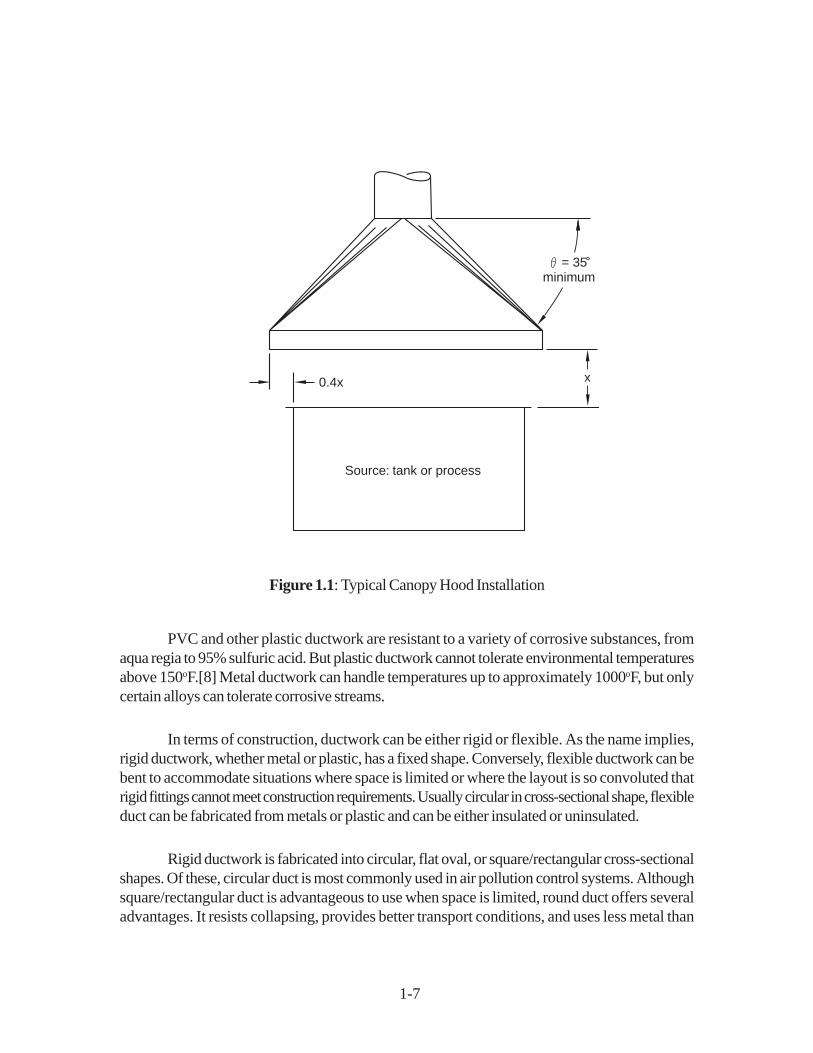
The last category is receptor hoods (passive or canopy hoods). A receptor hood typicallyis located above or beside a source, to collect the emissions, which are given momentum by thesource. For example, a canopy hood might be situated directly above an open tank containing ahot liquid (a buoyant source). With entrained air, vapors emitted from the liquid would rise into thehood. Here, the canopy hood would function as a passive collector, as the rising gases would bedrawn into the hood via natural draft. (See Figure 1.1.)

Receptor hoods are also used with nonbuoyant sources, sources from which emissions donot rise. But are “thrown off” from a process, such as a swing grinder. The initial velocity of theemissions typically is high enough to convey them into a receiving hood.[5]

1.2.2 Ductwork

Once the emission stream is captured by either a hood or a direct exhaust connection, it isconveyed to the control device via ductwork. The term “ductwork” denotes all of the equipmentbetween the capture device and the control device. This includes: (1) straight duct; (2) fittings,such as elbows and tees; (3) flow control devices (e.g., dampers); and (4) duct supports. Thesecomponents are described in Section 1.2.2.1.)

In air pollution control systems, the fan is usually located immediately before or after thecontrol device. Consequently, most of the ductwork typically is under a negative static pressure,varying from a few inches to approximately 20 inches of water column. These pressure conditionsdictate the type of duct used, as well as such design parameters as the wall thickness (gauge). Forinstance, welded duct is preferable to spiral-wound duct in vacuum applications.[6]

Ductwork is fabricated from either metal or plastic, the choice of material being dictatedby the characteristics of the waste gas stream, structural considerations, purchase and installationcosts, aesthetics, and other factors. Metals used include carbon steel (bare or galvanized), stainlesssteel, and aluminum. The most commonly used plastics are polyvinyl chloride (PVC) and fiberglass-reinforced plastic (FRP), although polypropylene (PP) and linear polyethylene (LPE) also can alsobe applied. However, one serious drawback to PP and LPE is that both are combustible.[7]

1-7

Figure 1.1: Typical Canopy Hood Installation

PVC and other plastic ductwork are resistant to a variety of corrosive substances, fromaqua regia to 95% sulfuric acid. But plastic ductwork cannot tolerate environmental temperaturesabove 150oF.[8] Metal ductwork can handle temperatures up to approximately 1000oF, but onlycertain alloys can tolerate corrosive streams.

In terms of construction, ductwork can be either rigid or flexible. As the name implies,rigid ductwork, whether metal or plastic, has a fixed shape. Conversely, flexible ductwork can bebent to accommodate situations where space is limited or where the layout is so convoluted thatrigid fittings cannot meet construction requirements. Usually circular in cross-sectional shape, flexibleduct can be fabricated from metals or plastic and can be either insulated or uninsulated.

Rigid ductwork is fabricated into circular, flat oval, or square/rectangular cross-sectionalshapes. Of these, circular duct is most commonly used in air pollution control systems. Althoughsquare/rectangular duct is advantageous to use when space is limited, round duct offers severaladvantages. It resists collapsing, provides better transport conditions, and uses less metal than

Source: tank or process

0.4x x

= 35minimum

1-8

square/rectangular or flat oval shapes of equivalent cross-sectional area.[9 ] Unless otherwisenoted, the following discussion pertains to rigid, circular duct, as this is the type most commonlyused in air pollution control.

Rigid metal circular duct is further classified according to method of fabrication. Longitudinalseam duct is made by bending sheet metal into a circular shape over a mandrel, and buttweldingthe two ends together. Spiral seam duct is constructed from a long strip of sheet metal, the edgesof which are joined by an interlocking helical seam that runs the length of the duct. This seam iseither raised or flush to the duct wall surface.

Fabrication method and cross-sectional shape are not the only considerations in designingductwork, however. One must also specify the diameter; wall thickness; type, number, and locationof fittings, controllers, and supports; and other parameters. Consequently, most ductworkcomponents are custom designed and fabricated, so as to optimally serve the control device.Some vendors offer prefabricated components, but these are usually common fittings (e.g., 90o

elbows) that are available only in standard sizes (e.g., 3- to 12-inch diameter).[10,11]

If either the gas stream temperature or moisture content is excessive, the ductwork mayneed to be insulated. Insulation inhibits heat loss/gain, saving energy (and money), on the one hand,and prevents condensation, on the other. Insulation also protects personnel who might touch theductwork from sustaining burns. There are two ways to insulate ductwork. The first is to installinsulation on the outer surface of the ductwork and cover it with a vapor barrier of plastic or metalfoil. The type and thickness of insulation used will depend on the heat transfer properties of thematerial. For instance, one vendor states that 4 inches of mineral wool insulation is adequate formaintaining a surface (“skin”) temperature of 140oF (the OSHA workplace limit) or lower, providedthat the exhaust gas temperature does not exceed 600oF. [12]

The second way to insulate ductwork is by using double-wall, insulated duct and fittings.Double-wall ductwork serves to reduce both heat loss and noise. One vendor constructs it from asolid sheet metal outer pressure shell and a sheet metal inner liner with a layer of fiberglass insulationsandwiched between. The insulation layer is typically 1-inch, although 2- and 3-inch thicknessesare available for more extreme applications. The thermal conductivities of these thicknesses are0.27, 0.13, and 0.09 Btu/hr-ft2-oF, respectively.[13]

1.2.2.1 Ductwork Components

As discussed above, a ductwork system consists of straight duct, fittings, flow controldevices, and supports. Straight duct is self-explanatory and easy to visualize. The “fittings” category,however, encompasses a range of components that perform one or more of the following functions:change the direction of the ducted gas stream, modify the stream velocity, tie it to another duct(s),facilitate the connection of two or more components, or provide for expansion/contraction whenthermal stresses arise.

1-9

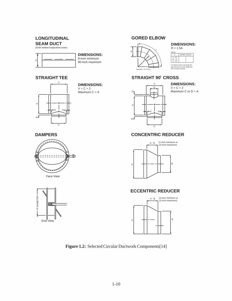
The most commonly used fittings are elbows (“ells”). These serve to change the gas streamdirection, typically by 30o, 45o, 60o, or 90o, though they may be designed for other angles as well.The elbow centerline radius determines the rate at which this directional change occurs. (SeeFigure 1.2.) The standard centerline radius (R

cl) is 1.5 times the elbow cross-sectional diameter

(Dc). However, in “long-radius” elbows, in which the directional change is more gradual than in

standard elbows, Rcl is greater than or equal to 2 times D

c.[14]

A T-shaped fitting (“tee”) is used when two or more gas streams must be connected. Instraight tees, the streams converge at a 90o angle, while in angle tees (“laterals”, “wyes”) theconnection is made at 30o, 45o, 60o, or some other angle. (See Figure 1.2.) Tees may have one“tap” (connection) or two, and may have either a straight or a “conical” cross-section at either orboth ends. Crosses are also used to connect duct branches. Here, the two branches intersect eachother at a right angle.

Reducers (commonly called “expansions” or “contractions”) are required whenever ductsof different diameter must be joined. Reducers are either concentric or eccentric in design. Inconcentric reducers, the diameter tapers gradually from the larger to smaller cross section. However,in eccentric reducers, the diameter decreases wholly on one side of the fitting.

Dampers control the volumetric flowrate through ventilation systems. They are usuallydelineated according to the flow control mechanism (single blade or multiblade), pressure rating(low/light or high/heavy), and means of control (manual or automatic). In single blade dampers, acircular plate is fastened to a rod, one end of which protrudes outside the duct. In the mostcommonly used type of single blade damper (butterfly type), this rod is used to control the gas flowby rotating the plate in the damper. Fully closed, the damper face sits perpendicular to the gas flowdirection; fully open, the face is parallel to the gas flow lines. Several single blade “control” dampersare depicted in Figure 1.2.

Blast gate dampers control the flow by sliding the damper blade in and out of the duct.Blast gates are often used to control the flow of air streams containing suspended solids, such as inpneumatic conveyors. In these respects, butterfly dampers and blast gates are analogous,respectively, to the globe valves and quick-opening gate valves that are used to regulate liquid flowin pipes.

Multiblade (louvered) dampers operate on the same principal as single blade dampers.However, instead of using a single blade or plate to control the gas flow, multiblade dampersemploy slats that open and close like venetian blinds.[15] Louvered dampers typically are used invery large ducts where a one-piece damper blade would be too difficult to move.

Manually-controlled dampers simply have a handle attached to the control rod which isused to adjust the gas flow by hand. If automatic control is needed, a pneumatic or electronic

1-10

Figure 1.2: Selected Circular Ductwork Components[14]

GORED ELBOWDIMENSIONS:�R = 1.5A

STRAIGHT TEE

CONCENTRIC REDUCER

ECCENTRIC REDUCER

DIMENSIONS:�V = C + 2�Maximum C = A

DIMENSIONS:�V = C + 2�Maximum C or D = A

Where:

Diameter 22 inches

Number of gores

2�3�5

LONGITUDINAL�SEAM DUCT

DIMENSIONS:�8-inch minimum�90-inch maximum

(Solid welded longitudinal seam)

A

For elbows where exceeds 90 , �add one gore for each additional�18 or fraction thereof.

0 - 35 �36 - 71 �72 - 90

A

R

<

A

C

1"

1" 1"

V

STRAIGHT 90 CROSS

A

C

1"

1"

1" 1"

V

D

DAMPERS

Face View

End View

"A" D

IAM

ET

ER

A B

A - B (1-inch minimum or �12-inch maximum)

A B

A - B (4-inch minimum or �12-inch maximum)

1-11

actuator is used. The actuator receives a pneumatic (pressurized air) or electrical signal from acontroller and converts it to mechanical energy which is used, in turn, to open/close the damper viathe damper rod. In this respect, an actuated damper is analogous to an automatic control valve.[16]For example, an automatic damper may be used to control the dilution air flow rate to an incineratorcombustion chamber. This flow rate, in turn, would depend on the combustibles concentration(i.e., percentage of lower explosive limit—%LEL) in the inlet waste gas stream. If this concentrationdeviates from a predetermined amount (“set point”), a signal is sent from the measuring device viathe controller to the automatic damper to increase/decrease the dilution air flow rate so as tomaintain the desired %LEL.

Expansion joints are installed, especially in longer metal duct runs, to allow the ductworkto expand or contract in response to thermal stresses. These fittings are of several designs. Onetype, the bellows expansion joint, consists of a piece of flexible metal (e.g., 304 stainless steel) thatis welded to each of two duct ends, connecting them. As the temperature of the duct increases, thebellows compresses; as the duct temperature decreases, the bellows expands. Another commonlyused expansion joint consists of two flanges between which is installed a section of fabric. Like thebellows expansion joint, it compresses as the duct temperature increases, and vice-versa. Thetemperature dictates the type of fabric used. For instance, silicone fiberglass and aramid fiber clothcan be used for duct temperatures of up to 500oF., while coated fiberglass cloth is needed toaccommodate temperatures of 1000oF.[17]

The last component to consider is the ductwork support system. However, it is far frombeing the least important. As the Sheet Metal and Air Conditioning Contractors’ National Association(SMACNA) HVAC Duct Construction Standards manual states, “The selection of a hangingsystem should not be taken lightly, since it involves not only a significant portion of the erectionlabor, but also because [the erection of] an inadequate hanging system can be disastrous.” As arule, a support should be provided for every 8 to 10 feet of duct run.[18] Ductwork can besuspended from a ceiling or other overhead structure via hangers or supported from below bygirders, pillars, or other supports.

A suspension arrangement typically consists of an upper attachment, a hanger, and a lowerattachment. The upper attachment ties the hanger to the ceiling, etc. This can be a concrete insert,an eye bolt, or a fastener such as a rivet or nailed pin. The hanger is generally a strap of galvanizedsteel, round steel rod, or wire that is anchored to the ceiling by the upper attachment. The type ofhanger used will be dictated by the duct diameter, which is proportional to its weight per lineal foot.For instance, wire hangers are only recommended for duct diameters up to 10 inches. For largerdiameters (up to 36 inches), straps or rods should be used. Typically, a strap hanger is run from theupper attachment, wrapped around the duct, and secured by a fastener (the lower attachment). Arod hanger also extends down from the ceiling. Unlike strap hangers, they are fastened to the ductvia a band or bands that are wrapped around the circumference. Duct of diameters greater than 3feet should be supported with two hangers, one on either side of the duct, and be fastened to two

1-12

circumferential bands, one atop and one below the duct.[19] Moreover, supports for larger ductworkshould also allow for both axial and longitudinal expansion and contraction, to accommodatethermal stresses.[20]

1.2.3 Stacks

Short stacks are installed after control devices to disperse the exhaust gases above groundlevel and surrounding buildings. As opposed to “tall” stacks, which can be up to 1,000 feet high,short stacks typically are no taller than 120 feet. Certain packaged control devices come equippedwith short (“stub”) stacks, with heights ranging from 30 to 50 feet. But if such a stack is neitherprovided nor adequate, the facility must erect a separate stack to serve one or more devices.Essentially, this stack is a vertical duct erected on a foundation and supported in some manner. Forstructural stability, the diameter of the stack bottom is slightly larger than the top diameter, whichtypically ranges from 1 to 7 feet.[21]

A short stack may be fabricated of steel, brick, or plastic (e.g., fiberglass-reinforcedplastic, or FRP). A stack may be lined or unlined. The material selection depends on the physicaland chemical properties of the gas stream, such as corrosiveness and acidity, as well as thetemperature differential between the gas stream and the ambient air. Liners of stainless steel, brick,or FRP usually are used to protect the stack against damage from the gas stream. They are mucheasier and less expensive to replace than the entire stack. Alternatively, the interior of an unlinedstack may be coated with zinc (galvanized), aluminum, or another corrosion-resistant material, buta coating does not provide the same protection as a liner and does not last as long.

Short stacks are either self-supporting (free-standing), supported by guy wires, or fastenedto adjacent structures. The type of support used depends on the stack diameter, height and weight,the wind load, local seismic zone characteristics, and other factors.

Auxiliary equipment for a typical stack includes an access door, a sampling platform,ladders, lightning protection system, and aircraft warning lights. The access door allows for removalof any accumulated materials at the bottom of the stack and provides access to the liner for repairor replacement. Local and state air pollution control regulations also may require the permanentinstallation of sampling platforms for use during periodic compliance tests, while ladders are usedboth during stack sampling and maintenance procedures. The lightning protection system is neededto prevent damage to the stack and immediate surroundings during electrical storms. Lastly, aircraftwarning lights are required by local aviation authorities.[23] Altogether, these auxiliaries can add alarge amount to the base stack cost.

1-13

1.3 Design Procedures

As stated above, a hood, ductwork, and a stack are key elements in any air pollutioncontrol system. Because each of these elements is different, both in appearance and function, eachmust be designed separately. But at the same time, these elements comprise a system, which isgoverned by certain physical laws that serve to unite these elements in “common cause.” Thus,before the individual design procedures for hoods, ductwork, and stacks are described, ventilationfundamentals will be presented. These fundamentals will cover basic fluid flow concepts and howthey may be applied to air pollution control ventilation systems. Nonetheless, these concepts willbe given as straightforwardly as possible, with the aim of making the design parameters easy tounderstand and compute.

1.3.1 Design Fundamentals

1.3.1.1 The Bernoulli Equation

The flow of fluids in any hood, duct, pipe, stack, or other enclosure is governed by asingle relationship, the familiar Bernoulli equation. Put simply and ideally, the Bernoulli equationstates that the total mechanical energy of an element of flowing fluid is constant throughout thesystem. This includes its potential energy, kinetic energy, and pressure energy. However, as nosystem is ideal, the Bernoulli equation must be adjusted to take into account losses to thesurroundings due to friction. Gains due to the energy added by fans, pumps, etc., also must beaccounted for. For a pound mass (lb

m) of fluid flowing in a steady-state system the adjusted

Bernoulli equation is:[24]

(1.1)

wherev = specific volume of fluid (ft3/lb

m)

p = static pressure—gauge (lbf/ft2)

z = height of fluid above some reference point (ft)u = fluid velocity through duct, hood, etc. (ft/sec)g = gravitational acceleration (ft/sec2)g

c= gravitational constant (32.174 ([lb

m-ft/sec2]/lb

f)

W = work added by fan, etc. (ft-lbf/lb

m)

F = energy lost due to friction (ft-lbf/lb

m)

( )vdp +

g

g

u

gW F

c c

∆∆

z

+∫ = −

2

12

2

1-14

Each of the terms on the left hand side of Equation 1.1 represents an energy change to apound mass of fluid between two locations in the system—points “1” and “2.” The work (W) andfriction (F) terms denote the amounts of energy added/lost between points 1 and 2.

Note that the units of each term in Equation 1.1 are “ft-lbf/lb

m,” energy per unit mass. In the

English system of units, “lbf” and “lb

m” are, for all intents, numerically equivalent, since the ratio of

the gravitational acceleration term (g) to the gravitational constant (gc) is very close to 1. In effect

the equation unit are “feet of fluid” or “fluid head in feet.” In air pollution control situations, the fluidoften has the properties of air. That is because the contaminants in the waste gas stream arepresent in such small amounts that the stream physical properties approximate those of pure air.

Because air is a “compressible” fluid, its specific volume is much more sensitive to changesin pressure and temperature than the specific volume of such “incompressible” fluids such as water.Hence, the “vdp” term in Equation 1.1 has to be integrated between points 1 and 2. However, inmost air pollution control ventilation systems neither the pressure nor the temperature changesappreciably from the point where the emissions are captured to the inlet of the control device.Consequently, the specific volume is, for all practical purposes, constant throughout the ventilationsystem, and one does not have to integrate the vdp term. With this assumption, the first term inEquation 1.1 becomes simply:

vdp dp p1

2

1

2

∫ ∫ = v = v∆ (1.2)

Illustration: VOC emitted by an open tank is captured by a hood and conveyed, via a blower,through 150 feet of 12-inch diameter ductwork to a refrigerated condenser outdoors. The blower,which moves the gas through the hood, ductwork, and condenser, is located immediately beforethe inlet to the condenser. Thus, the entire ventilation system is under vacuum. The stream temperatureand absolute pressure are 100oF and approximately 1 atmosphere (14.696 lb

f/in2), respectively.

The elevation of the refrigerated condenser inlet is 30 feet below that of the tank. The air velocityat the source is essentially zero, while the duct transport velocity is 2,000 ft/min. The static gaugepressure increases from -0.50 in. w.c. (water column) at the source to 4.5 in. w.c. at the bloweroutlet. Finally, the calculated friction loss through the ductwork and hood totals 1.25 in. w.c.Calculate the amount of mechanical energy that the blower adds to the gas stream. Assume thatthe gas temperature remains constant throughout.

Solution:

First, develop a factor to convert “inches of water” to “feet of air”:

F eet o f a ir = (Inches o f w a ter) ft

in

v

va

w

1

12100

100

(1.3)

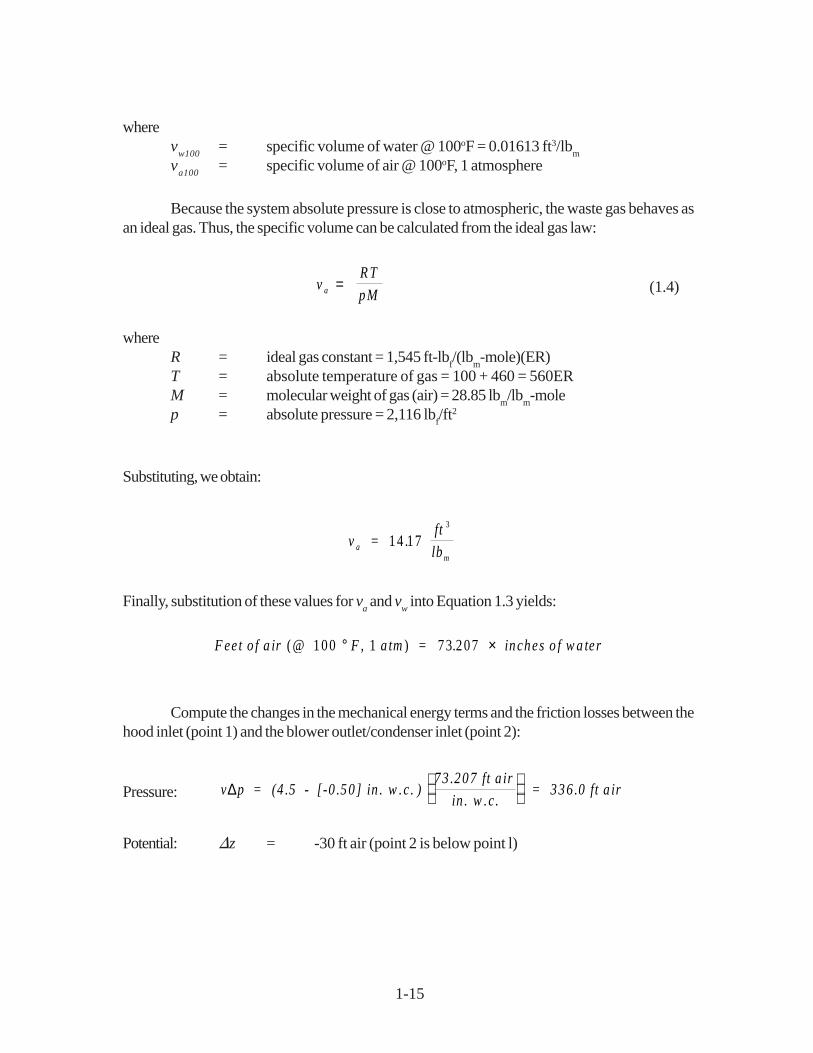
1-15

wherev

w100= specific volume of water @ 100oF = 0.01613 ft3/lb

m

va100

= specific volume of air @ 100oF, 1 atmosphere

Because the system absolute pressure is close to atmospheric, the waste gas behaves asan ideal gas. Thus, the specific volume can be calculated from the ideal gas law:

vR T

pMa = (1.4)

whereR = ideal gas constant = 1,545 ft-lb

f/(lb

m-mole)(ER)

T = absolute temperature of gas = 100 + 460 = 560ERM = molecular weight of gas (air) = 28.85 lb

m/lb

m-mole

p = absolute pressure = 2,116 lbf/ft2

Substituting, we obtain:

v a = ft

lb m

14 173

.

Finally, substitution of these values for va and v

w into Equation 1.3 yields:

F ee t o f a ir @ F , a tm = inches o f w a ter( ) .100 1 73 207° ×

Compute the changes in the mechanical energy terms and the friction losses between thehood inlet (point 1) and the blower outlet/condenser inlet (point 2):

Pressure: v p ∆ = (4 .5 - [-0 .50] in . w .c . ) 73 .207 ft a ir

in . w .c . = 336 .0 ft a ir

Potential: �z = -30 ft air (point 2 is below point l)

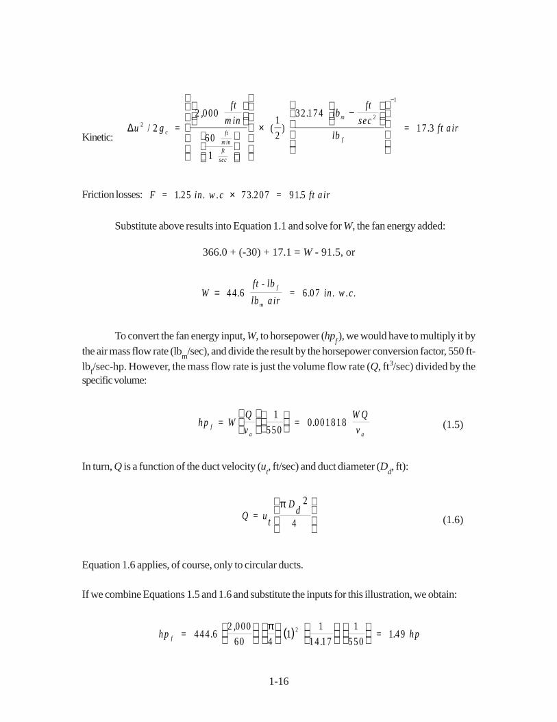
1-16

Kinetic:��∆u g

, ft

.c2

2

1

22 000

60

1

2

32 17417 3/ (

1)

. =

ft

m in

lb

seclb

= ft a irft

m inft

sec

m

f

×−

−

Friction losses: F . . .= in . w .c = ft a ir1 25 73 207 91 5×

Substitute above results into Equation 1.1 and solve for W, the fan energy added:

366.0 + (-30) + 17.1 = W - 91.5, or

W .= ft - lb

lb a ir = in . w .c .

f

m

44 6 6 07.

To convert the fan energy input, W, to horsepower (hpf ), we would have to multiply it by

the air mass flow rate (lbm/sec), and divide the result by the horsepower conversion factor, 550 ft-

lbf/sec-hp. However, the mass flow rate is just the volume flow rate (Q, ft3/sec) divided by thespecific volume:

hp = WQ

v

.f

a

1

5500 001818 =

W Q

v a(1.5)

In turn, Q is a function of the duct velocity (ut, ft/sec) and duct diameter (D

d, ft):

Q = ut

dπ D 2

4

(1.6)

Equation 1.6 applies, of course, only to circular ducts.

If we combine Equations 1.5 and 1.6 and substitute the inputs for this illustration, we obtain:

( )hp .,

..f = = hp444 6

2 000

60 41

1

14 17

1

5501 492

π

1-17

Some observations about this illustration:

• Recall that the precise units for W and the other terms in Equation 1.1 are “ft-lbf per

bmair,” which, for convenience, have been shortened to “ft air”. Thus, they measure

energy, not length.

• Compared to the pressure energy and friction terms, the potential and kinetic energy termsare small. Had they been ignored, the results would not have changed appreciably.

• The large magnitude of the pressure and friction terms clearly illustrates the importance ofkeeping one’s units straight. As shown in step (1), one inch of water is equivalent to over73 feet of air. However, as Equation 1.3 indicates, the pressure corresponding to equivalentheights of air and water columns would be the same.

• The fan power input depends not just on the total “head” (ft air) required, but also on thegas flow rate. Also, note that the horsepower computed via Equation 2.5 is a theoreticalvalue. It would have to be adjusted to account for the efficiencies of the fan and fan motor.The fan efficiency ranges from 40 to 70 percent, while the motor efficiency is typically 90percent. These efficiencies are usually combined into a single efficiency (�, fraction), bywhich the theoretical horsepower is divided to obtain the actual horsepower requirement.

1.3.1.2 Pressure: Static, Velocity, and Total

Although it is more rigorous and consistent to express the Bernoulli equation terms interms of feet of air (or, precisely, ft-lb

f/lb

m of air), industrial ventilation engineers prefer to use the

units “inches of water column (in. w.c.).” These units were chosen because, as the above illustrationshows, results expressed in “feet of air” are often large numbers that are cumbersome to use. Inaddition, the total pressure changes in ventilation systems are relatively small, compared to those inliquid flow systems. Total pressure changes expressed in inches of mercury would be small numberswhich are just as awkward to work with as large numbers. Hence, “inches of water” is a compromise,as values expressed in this measurement unit typically range from only 1 to 10. Moreover, practicalmeasurement of pressure changes is done with water-filled manometers.

In the previous paragraph, a new quantity was mentioned, total pressure (TP). Also knownas the “impact pressure”, the total pressure is the sum of the static gauge (SP) and velocity pressures(VP) at any point within a duct, hood, etc., all expressed in in. w.c.[25] That is:

T P = SP + V P (1.7)

1-18

where

SP = (cf)vpVP = (cf)u2/2g

c

The “cf” in the expressions for SP and TP is the factor for converting the energy termsfrom “ft air” to “in. w.c.”, both at standard temperature and absolute pressure (70oF, 1 atmosphere).(Again, keep in mind that, regardless of what units SP or VP are expressed in, the actual units are“energy per unit mass.”) This conversion factor, cf, would be obtained via rearranging Equation1.3:

cf = in .w .c

ft a ir =

v

vw

a

.

.12 70

70

(1.8)

where

vw70

= specific volume of water at 70oF = 0.01605 (ft3/lbm)

va70

= specific volume of air at 70oF = 13.41 (ft3/lbm)

Thus: cf = 0.01436 in. w.c./ft air

Clearly, the conversion factor varies as a function of temperature and pressure. For instance,at 100oF and 1 atmosphere, cf = 1/73.207 = 0.01366.

Conspicuously absent from Equation 1.7 is the potential energy term, “z(g/gc)”. This

omission was not inadvertent. In ventilation systems, the potential energy (P.E.) is usually smallcompared to the other terms. (For example, see illustration above.) The P.E. is, of course, afunction of the vertical distance of the measurement point in question from some datum level,usually the ground. At most, that distance would amount to no more than 20 or 30 feet, correspondingto a P.E. of approximately 0.3 to 0.4 in. w.c. Consequently, we can usually ignore the P.E.contribution in ventilation systems without introducing significant error.

The static gauge pressure in a duct is equal in all directions, while the velocity pressure, afunction of the gas velocity, varies across the duct face. The duct velocity is highest at the centerand lowest at the duct walls. However, for air flowing in a long, straight duct, the average velocityacross the duct (u

t) approximates the center line velocity (u

cl).[26] This is an important point, for

the average duct velocity is often measured by a pitot tube situated at the center of the duct.

1-19

By substituting for cf in Equation 1.7, we can obtain a simple equation that relates velocityto velocity pressure (VP) at standard conditions:

V P = . u

gt

c

0 0143

2

2

(1.9)

Solving:

u ft

sec V Pt

= . /66 94 1 2( ) (1.10)

Or:

u ,t /ft

m in = V P

4 016 1 2( ) (1.11)

Incidentally, these equations apply to any duct, regardless of its shape.

As Burton describes it, static gauge pressure can be thought of as the “stored” energy in aventilation system. This stored energy is converted to the kinetic energy of velocity and the lossesof friction (which are mainly heat, vibration, and noise). Friction losses fall into several categories:[27]

• Losses through straight duct

• Losses through duct fittings—elbow tees, reducers, etc.

• Losses in branch and control device entries

• Losses in hoods due to turbulence, shock, vena contracta

• Losses in fans

• Losses in stacks

These losses will be discussed in later sections of this chapter. Generally speaking, muchmore of the static gauge pressure energy is lost to` friction than is converted to velocity pressureenergy. It is customary to express these friction losses (�SP

f ) in terms of the velocity pressure:

F = SP = kV Pf ∆ (1.12)

1-20

where

k = experimentally-determined loss factor (unitless)

Alternatively, Equations 1.11 and 1.12 may be combined to express F (in. w.c.) in termsof the average duct velocity, u

t (ft/min):

F t= ku(6 .200 10 )-8× 2 (1.13)

1.3.1.3 Temperature and Pressure Adjustments

Equations 1.8 to 1.13 were developed assuming that the waste gas stream was at standardtemperature and pressure. These conditions were defined as 70oF and 1 atmosphere (14.696 lb

f/

in2), respectively. While 1 atmosphere is almost always taken as the standard pressure, severaldifferent standard temperatures are used in scientific and engineering calculations: 32oF, 68oF, and77oF, as well as 70oF. The standard temperature selected varies according to the industry orengineering discipline in question. For instance, industrial hygienists and air conditioning engineersprefer 70oF as a standard temperature, while combustion engineers prefer 77oF.

Before these equations can be used with waste gas streams which are not at 70oF and 1atmosphere, their variables must be adjusted. As noted above, waste gas streams in air pollutioncontrol applications obey the ideal gas law. From this law the following adjustment equation can bederived:

QT

T

P

P2 12

1

1

2

= Q

(1.14)

whereQ

2,Q

1 = gas flow rates at conditions 2 and 1, respectively (actual ft3/min)

T2,T

1 = absolute temperatures at conditions 2 and 1, respectively (oR)

P2,P

1 = absolute pressures at conditions 2 and 1, respectively (atm)

However, according to Equation 1.6:

Q = u D

tdπ 2

4

1-21

If Equations 1.6 and 1.14 were combined, we would obtain:

uT

T

P

P

D

Dtd

d2 1

2

1

1

2

22

12 = u t

(1.15)

This last expression can be used to adjust ut in any equation, as long as the gas flow is in

circular ducts.

1.3.2 Hood Design Procedure

1.3.2.1 Hood Design Factors

When designing a hood, several factors must be considered:[28]

• Hood shape

• Volumetric flow rate

• Capture velocity

• Friction

Each of these factors and their interrelationships will be explained in this section.

As discussed in Section 1.2.1, the hood shape is determined by the nature of the sourcebeing controlled. This includes such factors as the temperature and composition of the emissions,as well as the dimensions and configuration of the emission stream. Also important are suchenvironmental factors as the velocity and temperature of air currents in the vicinity.

The hood shape partly determines the volumetric flow rate needed to capture the emissions.Because a hood is under negative pressure, air is drawn to it from all directions. Consider thesimplest type of hood, a plain open-ended duct. Now, envision an imaginary sphere surroundingthe duct opening. The center of this sphere would be at the center of the duct opening, while thesphere radius would be the distance from the end of the duct to the point where emissions arecaptured. The air would be drawn through this imaginary sphere and into the duct hood. Now, thevolume of air drawn through the sphere would be the product of the sphere surface area and thehood capture velocity, u

c:[29]

Q x= u c ( )4 2π (1.16)

1-22

where

x = radius of imaginary sphere (ft)

Equation 1.16 applies to a duct whose diameter is small relative to the sphere radius.However, if the duct diameter is larger, the capture area will have to be reduced by the crosssectionalarea of the duct (D

d), or:

Q x= u D

cd4

42 2

ππ

−

(1.17)

Similarly, if a flange were installed around the outside of the duct end, the surface areathrough which the air was drawn—and the volume flow rate—would be cut in half. That occursbecause the flange would, in effect, block the flow of air from points behind it. Hence:

Q x= u c ( )2 2π (1.18)

From these examples, it should be clear that the hood shape has a direct bearing on thegas flow rate drawn into it. But Equations 1.16 to 1.18 apply only to hoods with spherical flowpatterns. For other hoods, other flow patterns apply—cylindrical, planal, etc. We can generalizethis relationship between volumetric flow rate and hood design parameters as follows:

Q x Sh= f(u i , , ) (1.19)

where

“f(...)” denotes “function of...”“Sh” indicates hood shape factorsu

i = design velocity—capture, face, slot

Table 1.1 lists design equations for several commonly used hood shapes. As this table shows, Q isa function of x, the hood shape, and, in general, the capture velocity (u

c). In the case of a booth

hood, the design velocity is the hood face velocity (uf). For slotted side-draft and back-draft

hoods, the slot velocity (us) is the design velocity. In practice, both the hood face and slot velocities

are the same, as each measures the speed at which the gas passes through the hood inlet opening(s).

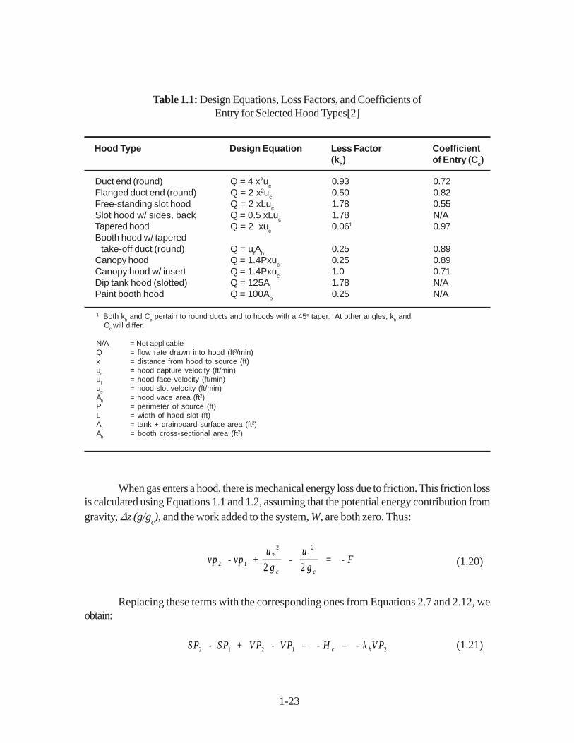
1-23

When gas enters a hood, there is mechanical energy loss due to friction. This friction lossis calculated using Equations 1.1 and 1.2, assuming that the potential energy contribution fromgravity, �z (g/g

c), and the work added to the system, W, are both zero. Thus:

vp - vp + u

g -

u

g = - F

c c2 1

22

12

2 2 (1.20)

Replacing these terms with the corresponding ones from Equations 2.7 and 2.12, weobtain:

SP 2 1 2 1 2 - SP + V P - V P = - H = - k V Pc h (1.21)

Duct end (round) Q = 4 x2uc

0.93 0.72Flanged duct end (round) Q = 2 x2u

c0.50 0.82

Free-standing slot hood Q = 2 xLuc

1.78 0.55Slot hood w/ sides, back Q = 0.5 xLu

c1.78 N/A

Tapered hood Q = 2 xuc

0.061 0.97Booth hood w/ tapered take-off duct (round) Q = u

fA

h0.25 0.89

Canopy hood Q = 1.4Pxuc

0.25 0.89Canopy hood w/ insert Q = 1.4Pxu

c1.0 0.71

Dip tank hood (slotted) Q = 125At

1.78 N/APaint booth hood Q = 100A

b0.25 N/A

Hood Type Design Equation Less Factor Coefficient(kh) of Entry (Ce)

1 Both kh and Cc pertain to round ducts and to hoods with a 45o taper. At other angles, kh and Cc will differ.

N/A = Not applicableQ = flow rate drawn into hood (ft3/min)x = distance from hood to source (ft)uc = hood capture velocity (ft/min)uf = hood face velocity (ft/min)us = hood slot velocity (ft/min)Ah = hood vace area (ft2)P = perimeter of source (ft)L = width of hood slot (ft)At = tank + drainboard surface area (ft2)Ab = booth cross-sectional area (ft2)

Table 1.1: Design Equations, Loss Factors, and Coefficients ofEntry for Selected Hood Types[2]

1-24

where

SPi

= static gauge pressure at point i (in. w.c.)

VPi

= velocity pressure at point i (in. w.c.)

Hc

= hood entry loss (in. w.c.)

kh

= hood loss factor (unitless)

In this equation, subscript 1 refers to a point just outside the hood face. Subscript 2denotes the point in the duct, just downstream of the hood, where the duct static pressure, SP

2 or

SPh and the duct transport velocity, u

2 or u

t are measured. At point 1, the hood velocity pressure,

VP1, is essentially zero, as the air velocity there is negligible. Moreover, the static gauge pressure,

SP1, will be zero, as the absolute pressure at point 1 is assumed to be at one atmosphere, the

reference pressure. After these simplifications are made, Equation 1.21 can be rearranged to solvefor the hood loss factor (k

h):

k - -SP

V P - h

h

2

1

(1.22)

At first glance, it appears that kh could be negative, since VP is always positive. However,

as the air entering the hood is under a vacuum created by a fan downstream, SPh must be negative.

Thus, the term “-SPh/VP

2” must be positive. Finally, because the absolute value of SP

h is larger

than VP2, k

h > 0.

The hood loss factor varies according to the hood shape. It can range from 0.04 for bellmouth hoods to 1.78 for various slotted hoods. A parameter related to the hood loss factor is thecoefficient of entry (c

e).[30] This is defined as:

c e = + k h

1

1

1 2

( )

/

(1.23)

ce depends solely on the shape of the hood, and may be used to compute k

h and related parameters.

Values of kh and c

e are listed in Table 1.1.

Illustration: The static gauge pressure, SPh, is -1.75 in. w.c. The duct transport velocity (u

t) is

3,500 ft/min. Calculate the loss factor and coefficient of entry for the hood. Assume standardtemperature and pressure.

1-25

Solution: First, calculate the duct velocity pressure. By rearranging Equation 1.11 and substitutingfor u

t, we obtain:

V P ,

,.=

u = = in . w .c .t

4 016

3 500

4 0160 76

2 2

,

Next, substitute for VP in Equation 1.22 and solve:

k- .

..h =

-SP

V P - = - - = h

1

1 75

0 761 1 30

Finally, use this value and Equation 1.23 to calculate the coefficient of entry:

C + .

.e = = 1

1 1 300 66

1 2

/

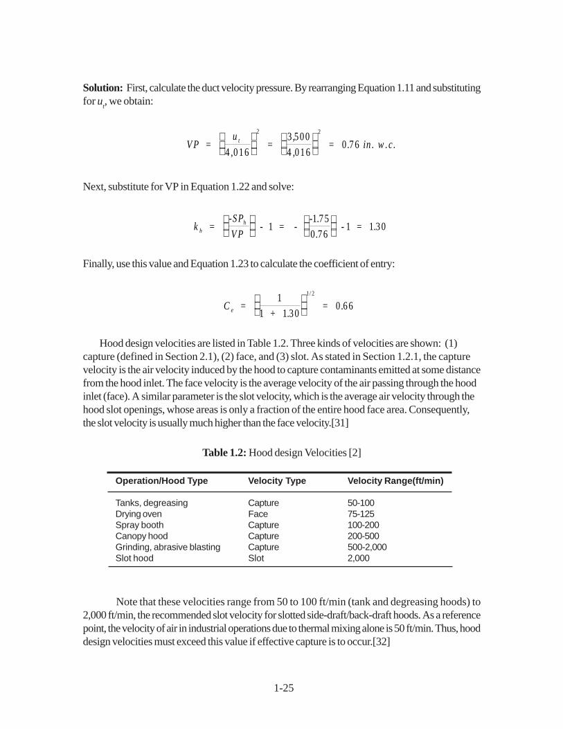
Hood design velocities are listed in Table 1.2. Three kinds of velocities are shown: (1)capture (defined in Section 2.1), (2) face, and (3) slot. As stated in Section 1.2.1, the capturevelocity is the air velocity induced by the hood to capture contaminants emitted at some distancefrom the hood inlet. The face velocity is the average velocity of the air passing through the hoodinlet (face). A similar parameter is the slot velocity, which is the average air velocity through thehood slot openings, whose areas is only a fraction of the entire hood face area. Consequently,the slot velocity is usually much higher than the face velocity.[31]

Table 1.2: Hood design Velocities [2]

Note that these velocities range from 50 to 100 ft/min (tank and degreasing hoods) to2,000 ft/min, the recommended slot velocity for slotted side-draft/back-draft hoods. As a referencepoint, the velocity of air in industrial operations due to thermal mixing alone is 50 ft/min. Thus, hooddesign velocities must exceed this value if effective capture is to occur.[32]

Operation/Hood Type Velocity Type Velocity Range(ft/min)

Tanks, degreasing Capture 50-100Drying oven Face 75-125Spray booth Capture 100-200Canopy hood Capture 200-500Grinding, abrasive blasting Capture 500-2,000Slot hood Slot 2,000

1-26

Two other velocities are also discussed in the industrial hygiene literature, although they donot have as much bearing on hood design as the capture, face, or slot velocities. These are theplenum velocity and the transport velocity. Plenum velocity is the velocity of the gas stream as itpasses through the tapered portion of a hood (plenum) between the hood opening and the ductconnection. This plenum is a transition area between the hood opening and duct. Consequently,the plenum velocity is higher than the hood face velocity, but lower than the duct (transport)velocity. The transport velocity- the gas velocity through the duct- varies according to the wastegas composition. It is a crucial parameter in determining the duct diameter, the static pressure loss,and the sizes of the system fan and fan motor. (For more on transport velocity, see Section 1.3.3.)

1.3.2.2 Hood Sizing Procedure

As with many control devices and auxiliaries, there are several approaches to sizing hoods.Some of these approaches are quite complex, entailing a series of complex calculations that yieldcorrespondingly accurate results. For instance, one hood sizing method in the literature involvesfirst determining the hood dimensions (length and width for rectangular hoods; diameter, for circular).The next step is to estimate the amount of metal plate area (ft2) required to fabricate a hood ofthese dimensions, via parametric curves. (No curves are provided for nonmetal hoods.) This platearea is input to an equation that includes a “pricing factor” and the per-pound price of metal. Thecost of labor needed to fabricate this hood is estimated from equations similar to the plate-arearelationships. Finally, the metal and labor costs are summed to obtain the total fabricated hoodcost.[33]

This method no longer yields reasonably accurate hood cost. Since the labor cost data areoutdated—1977 vintage—which makes them unescalatable. (The rule-of-thumb time limit forescalating costs is five years.) Even if the costs were up-to-date, the procedure is difficult to use,especially if calculations are made by hand.

A simpler sizing method—yet one sufficiently accurate for study estimating purposes—involves determining a single dimension, the hood face area (A

f). This area, identical to the hood

inlet area, can be correlated against the fabricated hood cost to yield a relatively simple costequation with a single independent variable. To calculate A

f, the following information is needed:

• Hood type

• Distance of the hood face from source (x)

• Capture (uc), face (u

f), or slot velocity (u

s)

• Source dimensions (for some hood types).

1-27

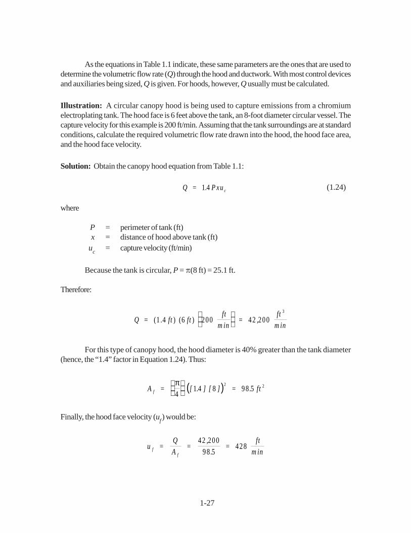
As the equations in Table 1.1 indicate, these same parameters are the ones that are used todetermine the volumetric flow rate (Q) through the hood and ductwork. With most control devicesand auxiliaries being sized, Q is given. For hoods, however, Q usually must be calculated.

Illustration: A circular canopy hood is being used to capture emissions from a chromiumelectroplating tank. The hood face is 6 feet above the tank, an 8-foot diameter circular vessel. Thecapture velocity for this example is 200 ft/min. Assuming that the tank surroundings are at standardconditions, calculate the required volumetric flow rate drawn into the hood, the hood face area,and the hood face velocity.

Solution: Obtain the canopy hood equation from Table 1.1:

Q .= P xu c1 4 (1.24)

where

P = perimeter of tank (ft)x = distance of hood above tank (ft)

uc

= capture velocity (ft/min)

Because the tank is circular, P = �(8 ft) = 25.1 ft.

Therefore:

Q , = ft ft ft

m in =

ft

m in(1 .4 ) (6 ) 200 42 200

3

For this type of canopy hood, the hood diameter is 40% greater than the tank diameter(hence, the “1.4” factor in Equation 1.24). Thus:

( )A . .f = [ ] [ ] = ftπ4

1 4 8 98 52 2

Finally, the hood face velocity (uf ) would be:

u,

.f = Q

A = =

ft

m inf

42 200

98 5428

1-28

In this example, note that the hood face velocity is higher than the capture velocity. This islogical, given the fact that the hood inlet area is smaller than the area through which the tank fumesare being drawn. The face velocity for some hoods is even higher. For example, for slotted hoodsit is at least 1,000 ft/min.[34] In fact, one vendor sizes the openings in his slotted hoods so as toachieve a slot velocity equal to the duct transport velocity.[35]

1.3.3 Ductwork Design Procedure

The design of ductwork can be an extremely complex undertaking. Determining the number,placement, and dimensions of ductwork components—straight duct, elbows, tees, dampers, etc.—can be tedious and time-consuming. However, for purposes of making study-level control systemcost estimates, such involved design procedures are not necessary. Instead, a much simplerductwork sizing method can be devised.

1.3.3.1 Two Ductwork Design Approaches

There are two commonly used methods for sizing and pricing ductwork. In the first, thetotal weight of duct is computed from the number and dimensions of the several components.Next, this weight is multiplied by a single price (in $/lb) to obtain the ductwork equipment cost. Todetermine the ductwork weight, one needs to know the diameter, length, and wall thickness ofevery component in the system. As stated above, obtaining these data can be a significant effort.

The second method is a variation of the first. In this technique, the ductwork componentsare sized and priced individually. The straight duct is typically priced as a function of length, diameter,wall thickness, and the material of construction. The elbows, tees, and other fittings are pricedaccording to all of these factors, except for length. Other variables, such as the amount and type ofinsulation, also affect the price. Because it provides more detail and precision, the second methodwill be used in this section.

1.3.3.2 Ductwork Design Parameters

Again, the primary ductwork sizing variable are length, diameter, and wall thickness. Anotherparameter is the amount of insulation required, if any.

Length: The length of ductwork needed with an air pollution control system depends on suchfactors as the distance of the source from the control device and the number of directional changesrequired. Without having specific knowledge of the source layout, it is impossible to determine thislength accurately. It could range from 20 to 2,000 feet or more. It is best to give the straight ductcost on a $/ft basis and let the reader provide the length. This length must be part of the specificationsof the emission source at which the ductwork is installed.

1-29

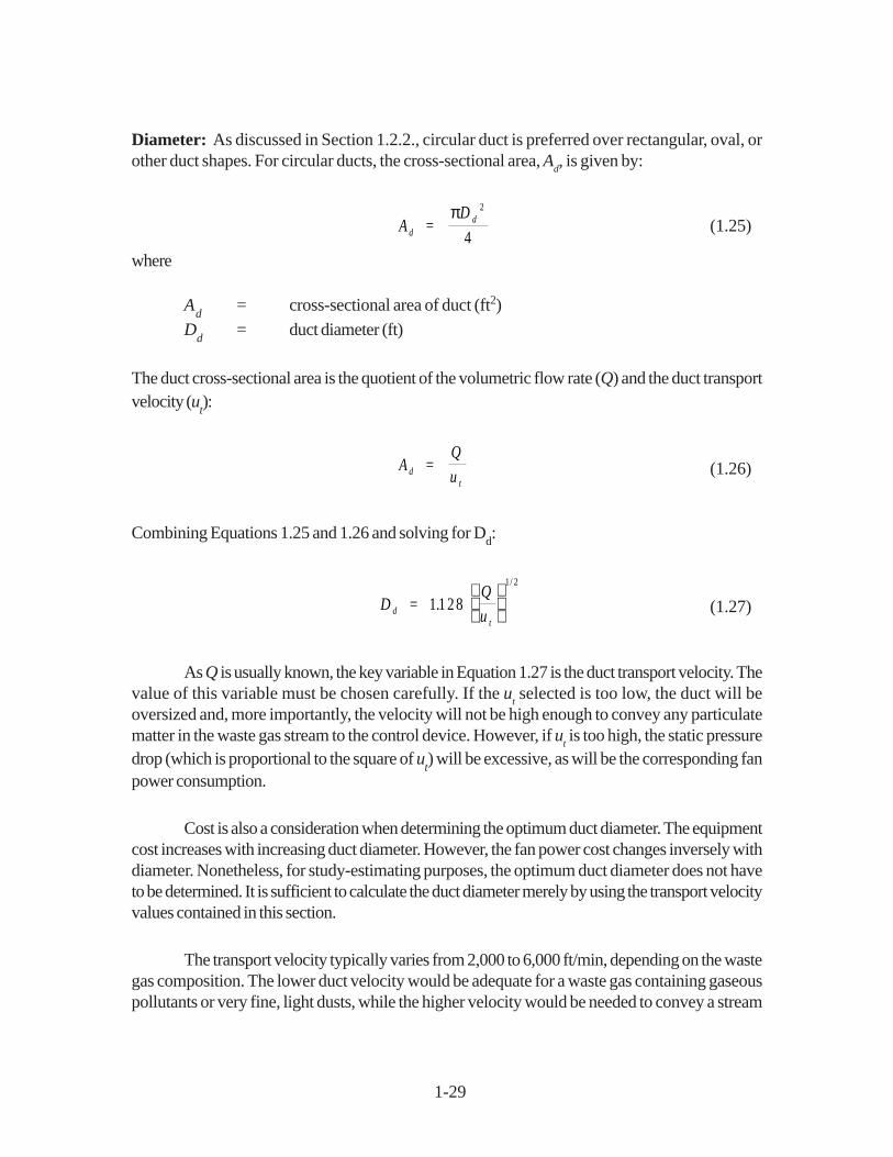
Diameter: As discussed in Section 1.2.2., circular duct is preferred over rectangular, oval, orother duct shapes. For circular ducts, the cross-sectional area, A

d, is given by:

A d = D dπ 2

4(1.25)

where

Ad

= cross-sectional area of duct (ft2)

Dd

= duct diameter (ft)

The duct cross-sectional area is the quotient of the volumetric flow rate (Q) and the duct transportvelocity (u

t):

A d = Q

u t(1.26)

Combining Equations 1.25 and 1.26 and solving for Dd:

D .d = Q

u t

1 128

1 2

/

(1.27)

As Q is usually known, the key variable in Equation 1.27 is the duct transport velocity. Thevalue of this variable must be chosen carefully. If the u

t selected is too low, the duct will be

oversized and, more importantly, the velocity will not be high enough to convey any particulatematter in the waste gas stream to the control device. However, if u

t is too high, the static pressure

drop (which is proportional to the square of ut) will be excessive, as will be the corresponding fan

power consumption.

Cost is also a consideration when determining the optimum duct diameter. The equipmentcost increases with increasing duct diameter. However, the fan power cost changes inversely withdiameter. Nonetheless, for study-estimating purposes, the optimum duct diameter does not haveto be determined. It is sufficient to calculate the duct diameter merely by using the transport velocityvalues contained in this section.

The transport velocity typically varies from 2,000 to 6,000 ft/min, depending on the wastegas composition. The lower duct velocity would be adequate for a waste gas containing gaseouspollutants or very fine, light dusts, while the higher velocity would be needed to convey a stream

1-30

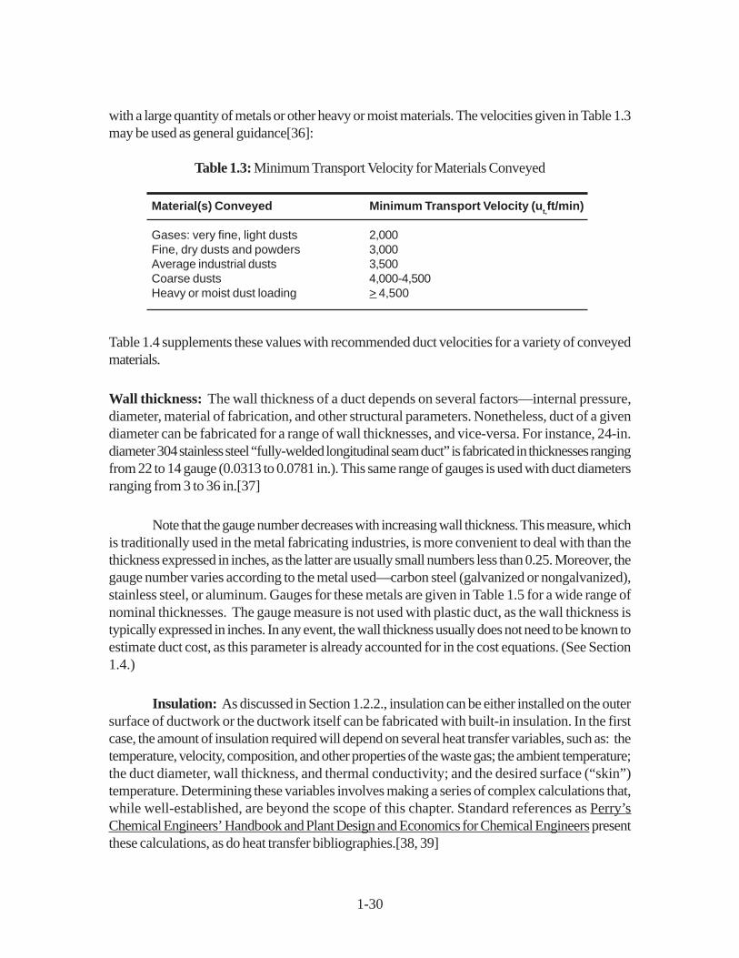
with a large quantity of metals or other heavy or moist materials. The velocities given in Table 1.3may be used as general guidance[36]:

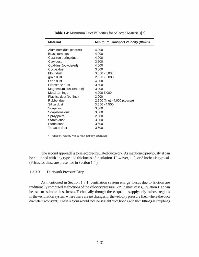
Table 1.3: Minimum Transport Velocity for Materials Conveyed

Table 1.4 supplements these values with recommended duct velocities for a variety of conveyedmaterials.

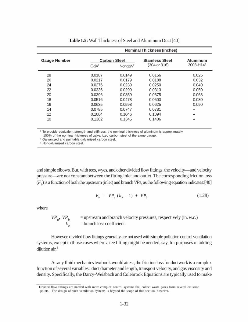
Wall thickness: The wall thickness of a duct depends on several factors—internal pressure,diameter, material of fabrication, and other structural parameters. Nonetheless, duct of a givendiameter can be fabricated for a range of wall thicknesses, and vice-versa. For instance, 24-in.diameter 304 stainless steel “fully-welded longitudinal seam duct” is fabricated in thicknesses rangingfrom 22 to 14 gauge (0.0313 to 0.0781 in.). This same range of gauges is used with duct diametersranging from 3 to 36 in.[37]

Note that the gauge number decreases with increasing wall thickness. This measure, whichis traditionally used in the metal fabricating industries, is more convenient to deal with than thethickness expressed in inches, as the latter are usually small numbers less than 0.25. Moreover, thegauge number varies according to the metal used—carbon steel (galvanized or nongalvanized),stainless steel, or aluminum. Gauges for these metals are given in Table 1.5 for a wide range ofnominal thicknesses. The gauge measure is not used with plastic duct, as the wall thickness istypically expressed in inches. In any event, the wall thickness usually does not need to be known toestimate duct cost, as this parameter is already accounted for in the cost equations. (See Section1.4.)

Insulation: As discussed in Section 1.2.2., insulation can be either installed on the outersurface of ductwork or the ductwork itself can be fabricated with built-in insulation. In the firstcase, the amount of insulation required will depend on several heat transfer variables, such as: thetemperature, velocity, composition, and other properties of the waste gas; the ambient temperature;the duct diameter, wall thickness, and thermal conductivity; and the desired surface (“skin”)temperature. Determining these variables involves making a series of complex calculations that,while well-established, are beyond the scope of this chapter. Standard references as Perry’sChemical Engineers’ Handbook and Plant Design and Economics for Chemical Engineers presentthese calculations, as do heat transfer bibliographies.[38, 39]

Material(s) Conveyed Minimum Transport Velocity (ut,ft/min)

Gases: very fine, light dusts 2,000Fine, dry dusts and powders 3,000Average industrial dusts 3,500Coarse dusts 4,000-4,500Heavy or moist dust loading > 4,500

1-31

The second approach is to select pre-insulated ductwork. As mentioned previously, it canbe equipped with any type and thickness of insulation. However, 1, 2, or 3 inches is typical.(Prices for these are presented in Section 1.4.)

1.3.3.3 Ductwork Pressure Drop

As mentioned in Section 1.3.1, ventilation system energy losses due to friction aretraditionally computed as fractions of the velocity pressure, VP. In most cases, Equation 1.12 canbe used to estimate these losses. Technically, though, these equations apply only to those regionsin the ventilation system where there are no changes in the velocity pressure (i.e., where the ductdiameter is constant). These regions would include straight duct, hoods, and such fittings as couplings

Table 1.4: Minimum Duct Velocities for Selected Materials[2]

Material Minimum Transport Velocity (ft/min)

Aluminum dust (coarse) 4,000Brass turnings 4,000Cast iron boring dust 4,000Clay dust 3,500Coal dust (powdered) 4,000Cocoa dust 3,000Flour dust 3,000 - 5,0001

grain dust 2,500 - 3,000Lead dust 4,000Limestone dust 3,500Magnesium dust (coarse) 3,000Metal turnings 4,000-5,000Plastics dust (buffing) 3,000Rubber dust 2,500 (fine) - 4,000 (coarse)Silica dust 3,500 - 4,500Soap dust 3,000Soapstone dust 3,000Spray paint 2,000Starch dust 3,000Stone dust 3,500Tobacco dust 3,500

1 Transport velocity varies with foundry operation.

1-32

1 Divided flow fittings are needed with more complex control systems that collect waste gases from several emission points. The design of such ventilation systems is beyond the scope of this section, however.

and simple elbows. But, with tees, wyes, and other divided flow fittings, the velocity—and velocitypressure—are not constant between the fitting inlet and outlet. The corresponding friction loss(F

b) is a function of both the upstream (inlet) and branch VPs, as the following equation indicates:[40]

Fb = V P k + V Pu b b( - 1 ) (1.28)

where

VPu, VP

b= upstream and branch velocity pressures, respectively (in. w.c.)

kb

= branch loss coefficient

However, divided flow fittings generally are not used with simple pollution control ventilationsystems, except in those cases where a tee fitting might be needed, say, for purposes of addingdilution air.1

As any fluid mechanics textbook would attest, the friction loss for ductwork is a complexfunction of several variables: duct diameter and length, transport velocity, and gas viscosity anddensity. Specifically, the Darcy-Weisbach and Colebrook Equations are typically used to make

Gauge Number Carbon Steel Stainless Steel AluminumGalv1 Nongalv2 (304 or 316) 3003-H143

Nominal Thickness (inches)

28 0.0187 0.0149 0.0156 0.02526 0.0217 0.0179 0.0188 0.03224 0.0276 0.0239 0.0250 0.04022 0.0336 0.0299 0.0313 0.05020 0.0396 0.0359 0.0375 0.06318 0.0516 0.0478 0.0500 0.08016 0.0635 0.0598 0.0625 0.09014 0.0785 0.0747 0.0781 --12 0.1084 0.1046 0.1094 --10 0.1382 0.1345 0.1406 --

1 To provide equivalent strength and stiffness, the nominal thickness of aluminum is approximately 150% of the nominal thickness of galvanized carbon steel of the same gauge.2 Galvanized and paintable galvanized carbon steel.3 Nongalvanized carbon steel.

Table 1.5: Wall Thickness of Steel and Aluminum Duct [40]

1-33

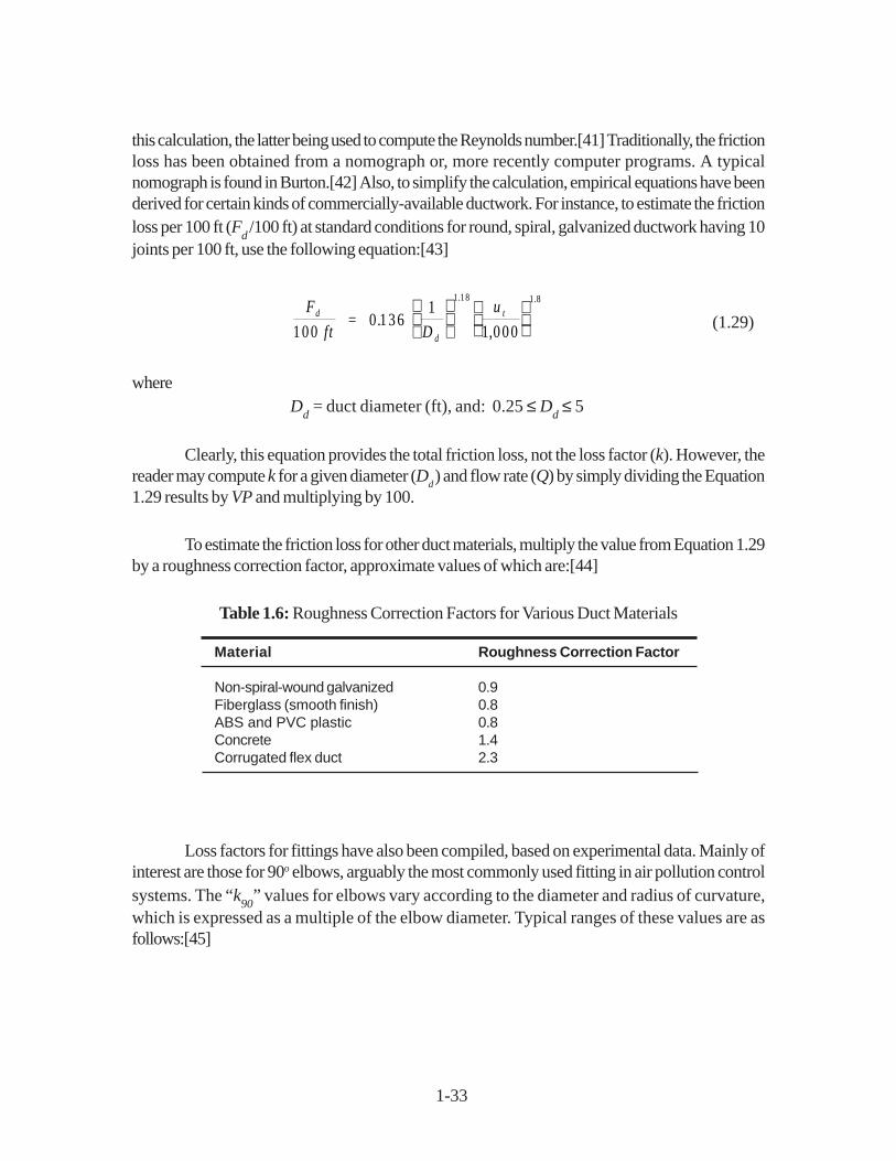
this calculation, the latter being used to compute the Reynolds number.[41] Traditionally, the frictionloss has been obtained from a nomograph or, more recently computer programs. A typicalnomograph is found in Burton.[42] Also, to simplify the calculation, empirical equations have beenderived for certain kinds of commercially-available ductwork. For instance, to estimate the frictionloss per 100 ft (F

d /100 ft) at standard conditions for round, spiral, galvanized ductwork having 10

joints per 100 ft, use the following equation:[43]

F.

D

ud

d

t

1000 136

1

1 000

1 18 1 8

ft =

. .

, (1.29)

whereD

d = duct diameter (ft), and: 0.25 ≤ D

d ≤ 5

Clearly, this equation provides the total friction loss, not the loss factor (k). However, thereader may compute k for a given diameter (D

d ) and flow rate (Q) by simply dividing the Equation

1.29 results by VP and multiplying by 100.

To estimate the friction loss for other duct materials, multiply the value from Equation 1.29by a roughness correction factor, approximate values of which are:[44]

Table 1.6: Roughness Correction Factors for Various Duct Materials

Loss factors for fittings have also been compiled, based on experimental data. Mainly ofinterest are those for 90o elbows, arguably the most commonly used fitting in air pollution controlsystems. The “k

90” values for elbows vary according to the diameter and radius of curvature,

which is expressed as a multiple of the elbow diameter. Typical ranges of these values are asfollows:[45]

Material Roughness Correction Factor

Non-spiral-wound galvanized 0.9Fiberglass (smooth finish) 0.8ABS and PVC plastic 0.8Concrete 1.4Corrugated flex duct 2.3

1-34

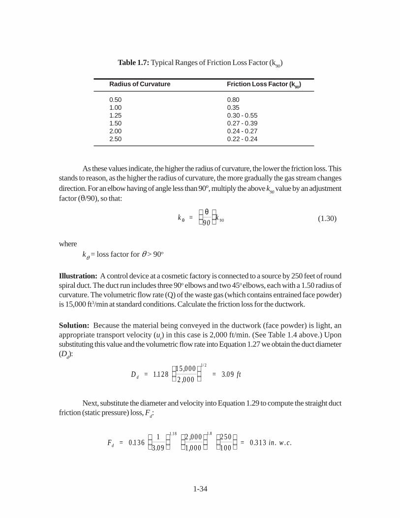
Table 1.7: Typical Ranges of Friction Loss Factor (k90

)

As these values indicate, the higher the radius of curvature, the lower the friction loss. Thisstands to reason, as the higher the radius of curvature, the more gradually the gas stream changesdirection. For an elbow having of angle less than 90o, multiply the above k

90 value by an adjustment

factor (�/90), so that:

k kθ

θ =

90

90 (1.30)

wherek� = loss factor for � > 90o

Illustration: A control device at a cosmetic factory is connected to a source by 250 feet of roundspiral duct. The duct run includes three 90o elbows and two 45o elbows, each with a 1.50 radius ofcurvature. The volumetric flow rate (Q) of the waste gas (which contains entrained face powder)is 15,000 ft3/min at standard conditions. Calculate the friction loss for the ductwork.

Solution: Because the material being conveyed in the ductwork (face powder) is light, anappropriate transport velocity (u

t) in this case is 2,000 ft/min. (See Table 1.4 above.) Upon

substituting this value and the volumetric flow rate into Equation 1.27 we obtain the duct diameter(D

d):

D . ,

,.d = = ft1 128

15 000

2 0003 09

1 2

/

Next, substitute the diameter and velocity into Equation 1.29 to compute the straight ductfriction (static pressure) loss, F

d:

F ..

,

,.d = = in . w .c .0 136

1

3 09

2 000

1 000

250

1000 313

1 18 1 8

. .

Radius of Curvature Friction Loss Factor (k90)

0.50 0.801.00 0.351.25 0.30 - 0.551.50 0.27 - 0.392.00 0.24 - 0.272.50 0.22 - 0.24

1-35

The 250/100 factor in this expression adjusts the friction loss from 100 feet (the basis ofequation 10.29) to 250 feet (the length of the duct system in this illustration). The rest of the frictionloss occurs through the five elbows (three 90o, two 45o), each with a 1.50 radius of curvature.These losses (F

c) are computed via Equation 1.12:

F V Pc = k θ (1.31)

where

VP = (2,000/4,016)2 (Equation 1.11, rearranged)= 0.248 in. w.c.

For the 90o elbows, k� = k

90 = 0.33 (average of table range), and:

Fc = 3 x 0.33 (0.248) = 0.246 in. w.c.

For the 45o elbows, k�= (45/90)k

90 = 0.165 (Equation 1.30), and:

Fc = 2 x 0.165(0.248) = 0.0818 in. w.c.

The total friction loss is, therefore:

F = 0.313 + 0.246 + 0.0818 = 0.641 in. w.c.

From this illustration, two observations may be made: (1) the static pressure loss throughthe straight duct is not large, even at this length (250 ft.) and (2) the losses through the elbows—which total 0.328 in. w.c.—are larger than the straight duct loss. Though it may be tempting toneglect fittings losses for the sake of expediency, doing so can cause a significant underestimationof the ventilation system static pressure loss.

1.3.4 Stack Design Procedures

As with ductwork, the design of stacks involves a number of stream, structural, and site-specific parameters.[46,47] These include:

Waste gas variables: inlet volumetric flow rate, temperature, and composition;

Site-specific data: elevation above sea level, ambient temperature fluctuations, topographic andseismic data, meteorological records, and building elevations and layout;

1-36

Structural parameters: thickness of stack wall and liner, location of breaching opening, type ofsupports, load capacity of foundation, modulus of resistance, and natural vibration frequency.

Fortunately, for study cost-estimating purposes, the only two stack design parameters thatneed to be determined are: (1) the stack diameter and (2) the stack height. The other variables(e.g., wall thickness) are incorporated into the equipment cost correlations. The stack diameter isrelatively easy to determine, as it depends primarily on waste stream conditions. The stack heightis more difficult to arrive at, as it is influenced by several site-specific variables. Nonetheless,ample guidance has been developed to allow the estimator to determine an acceptably accuratestack height.

1.3.4.1 Calculating Stack Diameter

Because most stacks have circular cross-sections, the stack diameter (Ds, ft) can be

calculated via the duct diameter formula (Equation 1.27):

D .s = Q

uc

c

1 128

1 2

/

(1.32)

where

uc

= stack exit velocity (ft/min)Q

c= exit volumetric flow rate (actual ft3/min)

It should be noted that the stack diameter in this formula is measured at the stack exit, notat the entrance. That is because, for structural reasons, the diameter at the bottom of the stacktypically is larger than the top diameter. Also note that the stack exit velocity does not necessarilyequal the duct transport velocity. Finally, Q

c may be different from the volumetric flow rate used to

size the ductwork. Because the stack always follows the control device, the flow rate entering thedevice may not equal the flow rate entering the stack, either in standard or actual ft3 /min terms.For instance, in a thermal incinerator, the outlet standard waste gas flow rate is almost alwayshigher than the inlet flow rate due to the addition of supplemental fuel.

The stack exit velocity, uc, affects the plume height, the distance that the plume rises above

the top of the stack once it exits. In a well-designed stack, uc should be 1.5 times the wind speed.

Typically, design exit velocities of 3,000 to 4,000 ft/min are adequate.[48] This range correspondsto wind speeds of 34 to 45 mi/hr.

1-37

1.3.4.2 Calculating Stack Height

Estimating the stack height is more difficult than calculating the stack exit diameter. Thestack height depends on several variables: the height of the source; the stack exit velocity; thestack and ambient temperatures; the height, shape, and arrangement of the nearby structures andterrain; and the composition of the stack outlet gas. Some of these variables are straightforward todetermine, while others (such as the dimensions and layout of nearby structures) are difficult todetermine without performing on-site modeling and monitoring studies.

The stack design height has two components: the height of the stack itself (Hs) and the

plume rise height (Hpr

) . Together these components comprise the effective stack height (He). That

is:

H e = H Hs pr+ (1.33)

However, the cost of the stack is a function of Hs alone. (See Section 1.4.) As discussed

above, the plume rise is a function of the stack exit velocity. It also depends on the temperaturedifferential between the stack gas and the ambient air. Specifically, a 1oF temperature differencecorresponds to approximately a 2.5-ft. increase in H

pr.[49]

For those sources subject to State Implementation Plans (SIPs), the stack height (Hs)

should be determined according to “good engineering practice” (GEP). GEP is defined as “theheight necessary to insure that emissions from the stack do not result in excessive concentrations ofany air pollutant in the immediate vicinity of the source as a result of atmospheric downwash,eddies, or wakes which may be created by the source itself, nearby structures, or nearby terrainobstacles.”[50] In this respect, GEP establishes the maximum allowable stack height credit forpurposes of calculating the ambient air quality impact of the emitting source. A source may build astack to any height, but only a certain amount of stack height will be allowed in determiningenvironmental impacts.[51]

For stacks constructed after January 12, 1979, the GEP stack height shall be the greaterof: (1) 65 meters (213 ft); (2) the height demonstrated by an approved fluid model or field studythat ensures that stack emissions do not cause excessive pollutant concentrations from atmosphericdownwash, wakes, eddy effects., etc; or (3) the height determined by the following equation:[52]

H .s = H + Lb 1 5 (1.34)

1-38

whereH

s= GEP stack height, measured from the ground level elevation at the stack

base (ft)

Hb

= height of nearby structure(s) measured from this ground level elevation (ft)

L = lesser dimension (height or projected width of nearby structure(s))

1.3.4.3 Calculating Stack Draft

As discussed previously, waste gas flowing through hoods and ductwork loses staticpressure due to friction. In the case of stacks, however, the gas stream can actually gain staticpressure, as a result of stack draft, which is the draft created by the stack gas-ambient air temperaturedifferential. Stack draft (SP

s, in. w.c.) can be calculated as follows:53

SP . T Ts

am b sa

= H H - s b r0 0341 1

( )− ×

ρ (1.35)

whereH

br = height of stack breaching (inlet duct connection) above stack base (ft)

P���= barometric pressure(in. w.c.)T

amb = ambient temperature (oR)

Tsa

= average stack gas temperature (oR)

Illustration: The waste gas from a thermal incinerator has an outlet flow rate and temperature of21,700 actual ft3/min. and 550oF, respectively. The maximum wind speed in the vicinity is 42 mi/hr,

while the stack exit and ambient temperatures are 450oF and 70oF, in turn. The barometric pressureis 1 atm. (29.92 in. Hg). The incinerator is near a 35-ft tall brick building, while the “projectedwidth” of an adjacent building is 40 ft. For a stack to disperse the incinerator offgas, calculate therequired: (1) exit velocity, (2) diameter, (3) height, and (4) draft.

Solution:

Exit velocity: According to the above guideline, the velocity should be 1.5 times the wind speed, or:

u . ,c = m ph fpm

m ph=

ft

m in1 5 42 88 5 540× × (1.36)

1-39

Stack diameter: The exit volumetric flow rate is measured at the stack exit temperature, namely450oF. However, the above flow rate was measured at 550oF, the incinerator outlet temperature.Correcting to the stack exit temperature, we obtain:

Q ,c = = ac tua l ft

m in

321 ,700 (450 + 460 )

(550 + 460 )

×19 600 (1.37)

Substituting this value into Equation 1.32:

D .,

,.s = = ft1 128

19 600

5 5402 12

1 2

/

Stack height: As a first approximation, estimate the GEP stack height from Equation 1.33,where the variables H

b and L are 35 ft and 40 ft, respectively:

Hs = 35 + 1.5(40) = 95 ft.

Clearly, this Hs is less than the GEP maximum height (213 ft), so it will be used in this example.

Stack draft: All of the inputs needed to compute the stack draft via Equation 1.35 are knownexcept the stack breaching height, H

br. However, a minimum of 5 ft is recommended for this

parameter.[54] This value will be used in this calculation. Also, the average stack temperature is:

T = Rsa = (450 + 550 )

2 + 460 960 ° (1.38)

Finally, the barometric pressure expressed in inches of water is:

ρ = in . H g in . w a ter

in . H g = in . w .c .29 92

13 6407.

.× (1.39)

Upon substitution, we obtain:

( ) ( ) ( )SP . - +

.s = - = in . w .c .0 034 118 5 4071

70 460

1

9601 32

1-40

1.4 Estimating Total Capital Investment

This section presents the information needed for estimating the total capital investment(TCI) for hoods, ductwork, and stacks. The TCI includes the equipment cost (EC) for the hood,ductwork, or stack; taxes; freight charges; instrumentation (if applicable); and direct and installationcosts. All costs are presented in second quarter 1993 dollars, and are of “study” estimate accuracy(± 30 percent).2 Moreover, the costs are for new facility installations; no retrofit costs are included.

The equipment costs are presented in Section 1.4.1, while the installation costs are shownin Section 1.4.2. In each of these sections, the three categories of equipment are covered inseparate subsections.

1.4.1 Equipment Costs

Several vendors provided costs (prices) for each of the three equipment categories. Theirresponses reflected a range of sizes, designs, and materials of construction. These prices havebeen correlated against some easy-to-determine design (sizing) parameter via least-squaresregression analysis. Each of these correlations pertains to a certain type of equipment (e.g., circularcanopy hoods) within a specified size range of the parameter in question (e.g., 2 to 200 ft2 inletarea). For that reason, a cost correlation should not be extrapolated outside the parameter rangespecified.

Some of the prices the vendors provided pertain to stock (“off-the-shelf”) items, whileother costs are for custom-fabricated equipment. Vendors tend to specialize in either stock orcustom items. Most hoods and stacks are custom-made, either fabricated in the vendor’s factoryor erected on-site. Conversely, ductwork components usually are stock items, though larger pieceshave to be custom-made. (Of course, there are exceptions to this.) Finally, all prices given in thefollowing section are “free-on-board (F.O.B.) vendor,” meaning that they include neither freightnor taxes.

1.4.1.1 Hood Costs

In all, four vendors provided prices for hoods.[55] These prices covered the followingtypes of hoods:

• Canopy—circular

• Canopy—rectangular

2 For information on escalating these prices to more current dollars, refer to the EPA report Escalation Indexes for Air Pollution Control Costs and updates thereto, all of which are installed on the OAQPS Technology Transfer Network

(CTC Bulletin Board).

1-41

• Push-pull

• Slide-draft

• Back-draft (slotted)

Descriptions and design procedures for these hoods are given in Sections 1.2.1 and 1.3.2,respectively. As explained in Section 1.3.2, hood costs have been found to correlate well with thehood inlet or face area (A

f, ft2). Furthermore, the functional form that best fits the cost-face area

correlation (equation) is the “power function,” or:

C hb = aA f (1.40)

whereC

h= hood cost ($)

a,b = equation regression parameters

The values of the equation parameters vary according to hood type and material ofconstruction. These parameters are shown in Table 1.8.

Illustration: What would be the cost of the electroplating tank canopy hood sized for the illustrationin Section 1.2.2. Assume that the hood is fabricated of FRP.

Solution: Recall that the face area (Af ) calculated for that hood was 98.5 ft2. Because this is a

circular canopy hood, the equation parameters from Table 1.8 are: a = 123 and b = 0.575. (Notethat this hood area falls within the equation range of 2 to 200 ft2.) Substituting these parametersinto Equation 1.40, we obtain:

Ch = 123(98.5)0.575 = $1,720.

1.4.1.2 Ductwork Costs

Several vendors provided ductwork prices, also for a range of sizes, materials, and designs.These prices covered the following equipment items:

Straight ductwork:Circular – Steel sheet (galvanized carbon, w/ & w/o insulation; 304 stainless;) – Steel plate (coated carbon; 304 stainless) – Plastic (FRP; PVC) Square – Steel (aluminized carbon; w/ & w/o insulation)

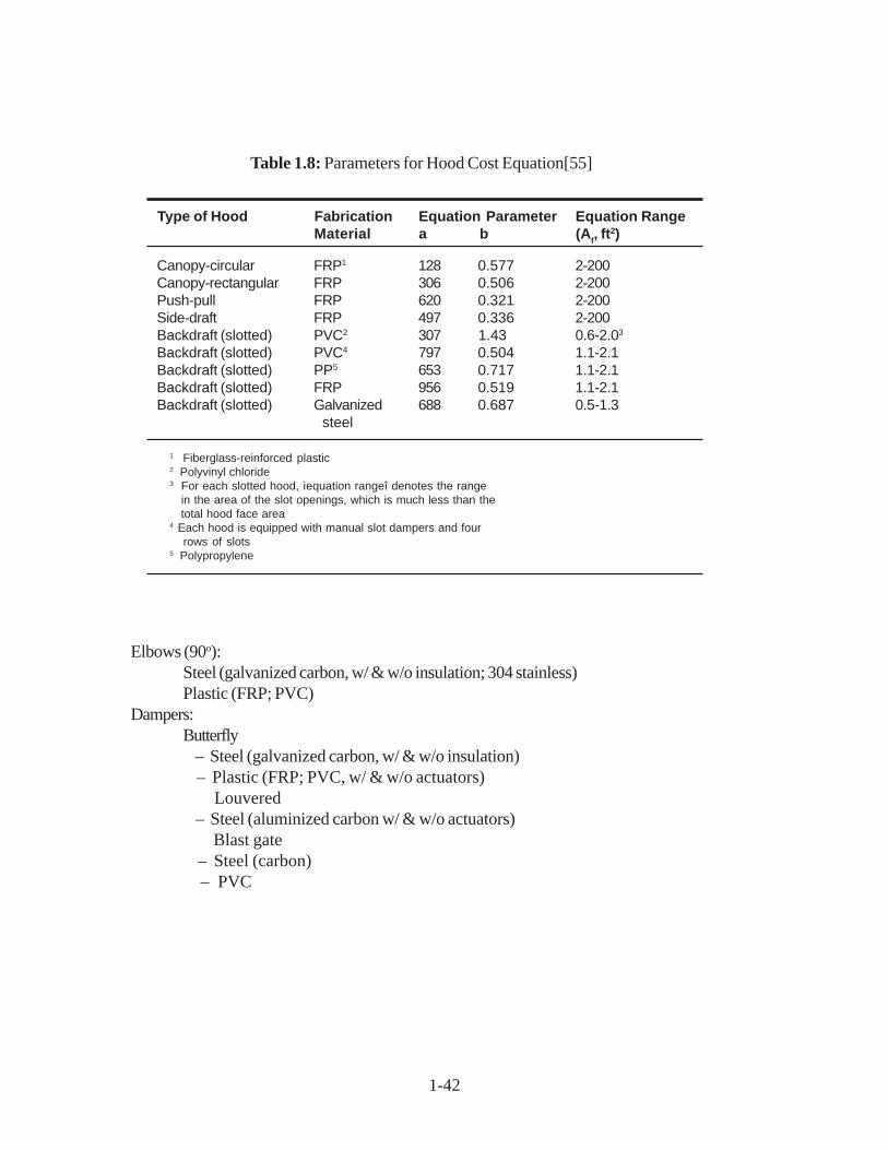
1-42

Elbows (90o):Steel (galvanized carbon, w/ & w/o insulation; 304 stainless)Plastic (FRP; PVC)

Dampers:Butterfly – Steel (galvanized carbon, w/ & w/o insulation) – Plastic (FRP; PVC, w/ & w/o actuators) Louvered – Steel (aluminized carbon w/ & w/o actuators) Blast gate – Steel (carbon) – PVC

Table 1.8: Parameters for Hood Cost Equation[55]

Canopy-circular FRP1 128 0.577 2-200Canopy-rectangular FRP 306 0.506 2-200Push-pull FRP 620 0.321 2-200Side-draft FRP 497 0.336 2-200Backdraft (slotted) PVC2 307 1.43 0.6-2.03

Backdraft (slotted) PVC4 797 0.504 1.1-2.1Backdraft (slotted) PP5 653 0.717 1.1-2.1Backdraft (slotted) FRP 956 0.519 1.1-2.1Backdraft (slotted) Galvanized 688 0.687 0.5-1.3

steel

Type of Hood Fabrication Equation Parameter Equation RangeMaterial a b (Af, ft

2)

1 Fiberglass-reinforced plastic2 Polyvinyl chloride3 For each slotted hood, ìequation rangeî denotes the range in the area of the slot openings, which is much less than the total hood face area4 Each hood is equipped with manual slot dampers and four rows of slots5 Polypropylene

1-43

These prices were regressed against the diameter of the equipment item (straight duct,elbow, or damper). The regression correlations were of three forms: power function (primarily),exponential, and linear. Equation 1.40 depicts the power function, while the other forms are:

( )E xp onen tia l C aei bD= (1.41)

( )L inear C = a + bDi (1.42)

whereC

i= cost of equipment item in question

a,b = regression parametersD = equipment diameter

The regression parameters are listed in Tables 1.9 to 1.11, along with the size applicabilityranges for the respective correlations. (Note: The correlations should not be extrapolated outsidethese ranges.) The following paragraphs contain additional information about the price data andthe correlations:

Straight duct: As indicated above, vendors provided prices for steel plate, steel sheet (spiral-wound and longitudinal seam), and plastic straight duct. The major difference between the twosteel duct types lies in the wall thickness. Steel plate duct typically has wall thicknesses of 3/16 in.to 1/2 in., while steel sheet duct wall thicknesses usually range from 28 gauge to 10 gauge. AsTable 1.5 shows, this range corresponds to wall thicknesses of 0.0149 in. to 0.1406 in., respectively,although the exact thicknesses will vary with the type of steel used (e.g., carbon vs. stainless).Also, as discussed in Section 1.3.3.2, each duct diameter can be fabricated with a range of wallthicknesses.

Most of the steel duct vendors supplied prices for a minimum and a maximum wall thickness for agiven diameter. However, to simplify matters for cost estimators, these “low” and “high” prices firstwere averaged, and then the average prices were regressed against the diameters. This averagingwas necessary, because those making study cost estimates usually do not have enough informationavailable to predict duct wall thicknesses.

Prices for both circular and square insulated steel sheet duct were among the data received.The insulated circular steel duct is “double-wall, spiral-wound” in construction, wherein the insulationis installed between the inner and outer walls. Costs were provided for both 1-in. and 3-in. fiberglassinsulation thicknesses. For the square duct, prices were given for a 4-in. thickness of mineral woolinsulation applied to the outer surface of the duct. The correlation parameters in Table 1.9 reflectthese specifications.

1-44

Dampers: Prices were obtained for three types of dampers: butterfly, louvered, and blast gates.The galvanized carbon steel butterfly dampers were priced with and without 1-in. fiberglassinsulation, while prices for the aluminized carbon steel louvered dampers were based on eithermanual or automatic control (via electric actuators). Similarly, the PVC butterfly dampers weremanual or equipped with pneumatic actuators. Both the carbon steel and the PVC blast gateswere manual. Correlation parameters for the steel and plastic dampers are shown in Tables 1.10and 1.11, in turn.

Prices for both carbon steel (galvanized, painted, or aluminized) and 304 stainless steelduct were received. The carbon steel duct is used in situations where “mild” steel is suitable, whilethe stainless steel duct is required whenever the gas stream contains high concentrations of corrosivesubstances.

Vendors gave prices for plastic (FRP and PVC) duct also (Table 1.11). However, for agiven diameter this duct is fabricated in a single wall thickness, which varies from approximately1/8 in. to 1/4 in. Consequently, the estimator is not required to select a wall thickness when costingplastic duct.

Elbows: Prices for steel sheet and plastic 90o elbows were also submitted. The steel sheet elbowswere “gored” (sectioned) elbows fabricated from five pieces of sheet metal welded together. Like

Illustration: A fabric filter handling 16,500 ft3/min of 200oF waste gas laden with noncorrosivecocoa dust is located 95 ft across from and 20 ft above, the emission source (a drying oven).Straight duct with four 90o elbows (all fabricated from spiral-wound, galvanized carbon steelsheet) and a butterfly damper (also galvanized CS) will be required to convey the gas from thesource to the control device. Assume that the ductwork contains 1-in. thick insulation to preventcondensation. Estimate the cost of these items.

Solution: First, determine the diameter of the straight duct, elbows, and damper. From Table 1.4,the minimum transport velocity (u

t) for cocoa dust is 3,000 ft/min. Substituting this value and the

gas volumetric flow rate into Equation 2.27, we obtain:

D .,

,. ft = . ind = = .1 128

16 500

3 0002 65 31 7

1 2

/

Next, obtain the costs of the ductwork items as follows:

Straight ductwork: From Table 1.9, select the equation parameters for galvanized circular spiral-wound duct (1-in. insulation) and substitute them and the diameter into the appropriate equationtype (power function, Equation 1.40).

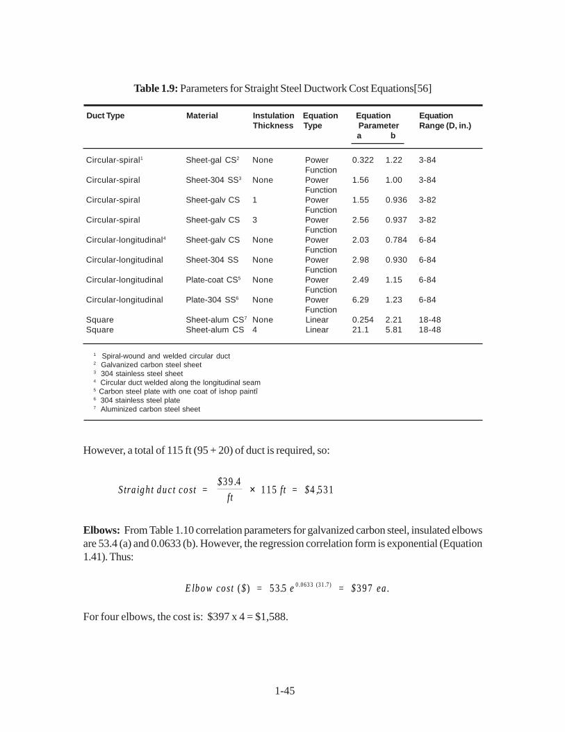
1-45

Table 1.9: Parameters for Straight Steel Ductwork Cost Equations[56]

Duct Type Material Instulation Equation Equation EquationThickness Type Parameter Range (D, in.)

a b

Circular-spiral1 Sheet-gal CS2 None Power 0.322 1.22 3-84 Function

Circular-spiral Sheet-304 SS3 None Power 1.56 1.00 3-84 Function

Circular-spiral Sheet-galv CS 1 Power 1.55 0.936 3-82 Function

Circular-spiral Sheet-galv CS 3 Power 2.56 0.937 3-82 Function

Circular-longitudinal4 Sheet-galv CS None Power 2.03 0.784 6-84 Function

Circular-longitudinal Sheet-304 SS None Power 2.98 0.930 6-84 Function

Circular-longitudinal Plate-coat CS5 None Power 2.49 1.15 6-84 Function

Circular-longitudinal Plate-304 SS6 None Power 6.29 1.23 6-84 Function

Square Sheet-alum CS7 None Linear 0.254 2.21 18-48Square Sheet-alum CS 4 Linear 21.1 5.81 18-48

1 Spiral-wound and welded circular duct2 Galvanized carbon steel sheet3 304 stainless steel sheet4 Circular duct welded along the longitudinal seam5 Carbon steel plate with one coat of ìshop paintî6 304 stainless steel plate7 Aluminized carbon steel sheet

However, a total of 115 ft (95 + 20) of duct is required, so:

S tra igh t duct co st = ft = $$ .

ft,

39 4115 4 531×

Elbows: From Table 1.10 correlation parameters for galvanized carbon steel, insulated elbowsare 53.4 (a) and 0.0633 (b). However, the regression correlation form is exponential (Equation1.41). Thus:

E lbow cost = = ea .( ) (31 .7 )$ . e $. 53 5 3970 063 3

For four elbows, the cost is: $397 x 4 = $1,588.

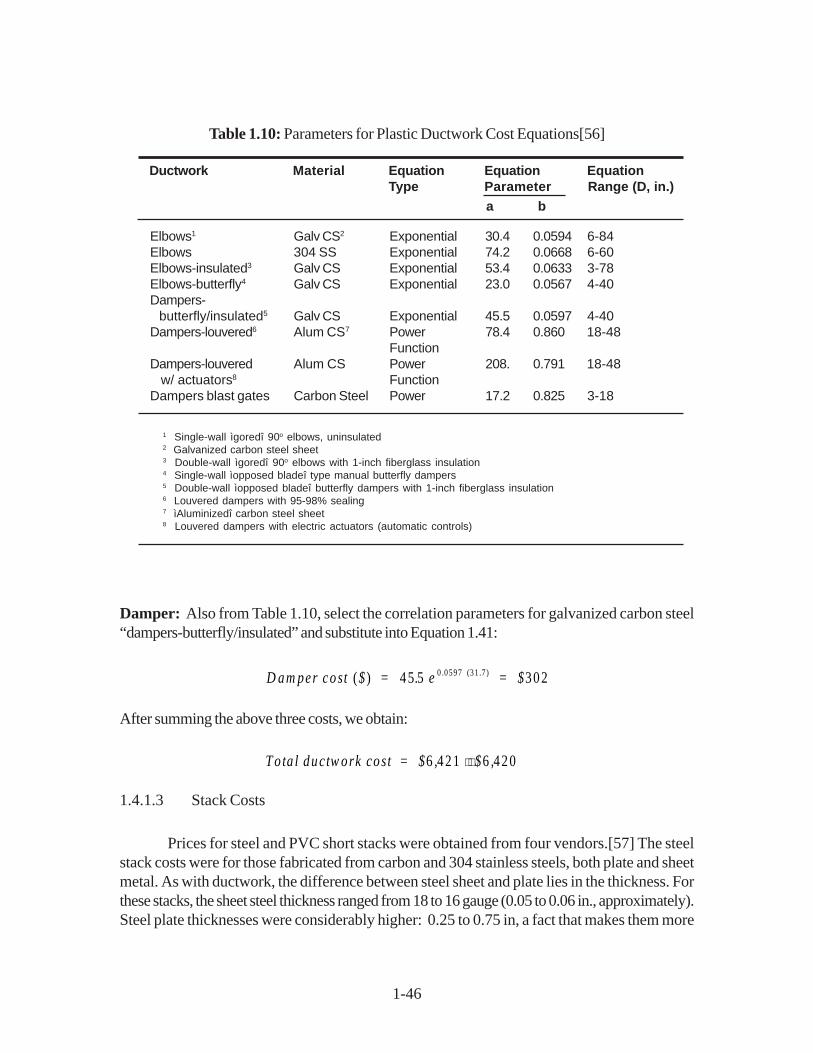
1-46

Table 1.10: Parameters for Plastic Ductwork Cost Equations[56]

Ductwork Material Equation Equation EquationType Parameter Range (D, in.)

Elbows1 Galv CS2 Exponential 30.4 0.0594 6-84Elbows 304 SS Exponential 74.2 0.0668 6-60Elbows-insulated3 Galv CS Exponential 53.4 0.0633 3-78Elbows-butterfly4 Galv CS Exponential 23.0 0.0567 4-40Dampers- butterfly/insulated5 Galv CS Exponential 45.5 0.0597 4-40Dampers-louvered6 Alum CS7 Power 78.4 0.860 18-48

FunctionDampers-louvered Alum CS Power 208. 0.791 18-48 w/ actuators8 FunctionDampers blast gates Carbon Steel Power 17.2 0.825 3-18

1 Single-wall ìgoredî 90o elbows, uninsulated2 Galvanized carbon steel sheet3 Double-wall ìgoredî 90o elbows with 1-inch fiberglass insulation4 Single-wall ìopposed bladeî type manual butterfly dampers5 Double-wall ìopposed bladeî butterfly dampers with 1-inch fiberglass insulation6 Louvered dampers with 95-98% sealing7 ìAluminizedî carbon steel sheet8 Louvered dampers with electric actuators (automatic controls)

a b

Damper: Also from Table 1.10, select the correlation parameters for galvanized carbon steel“dampers-butterfly/insulated” and substitute into Equation 1.41:

D am per cost = = $( ) (31 .7 )$ . e .45 5 3020 0597

After summing the above three costs, we obtain:

T o ta l ductw ork cost = $6 421 6 420, $ , ⟩⟩

1.4.1.3 Stack Costs

Prices for steel and PVC short stacks were obtained from four vendors.[57] The steelstack costs were for those fabricated from carbon and 304 stainless steels, both plate and sheetmetal. As with ductwork, the difference between steel sheet and plate lies in the thickness. Forthese stacks, the sheet steel thickness ranged from 18 to 16 gauge (0.05 to 0.06 in., approximately).Steel plate thicknesses were considerably higher: 0.25 to 0.75 in, a fact that makes them more

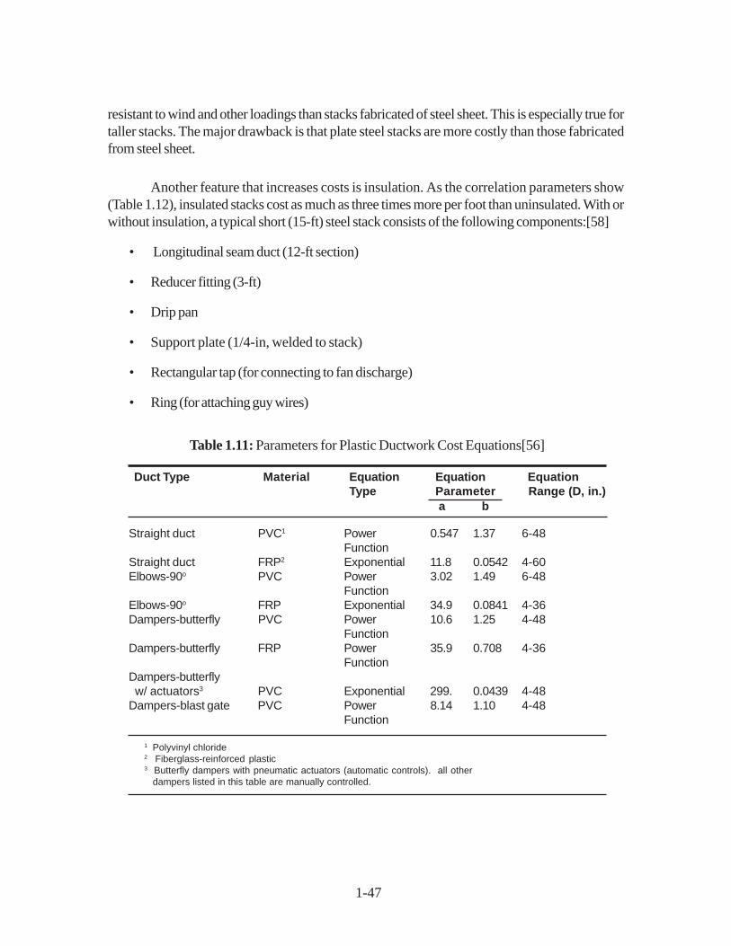
1-47

resistant to wind and other loadings than stacks fabricated of steel sheet. This is especially true fortaller stacks. The major drawback is that plate steel stacks are more costly than those fabricatedfrom steel sheet.

Another feature that increases costs is insulation. As the correlation parameters show(Table 1.12), insulated stacks cost as much as three times more per foot than uninsulated. With orwithout insulation, a typical short (15-ft) steel stack consists of the following components:[58]

• Longitudinal seam duct (12-ft section)

• Reducer fitting (3-ft)

• Drip pan

• Support plate (1/4-in, welded to stack)

• Rectangular tap (for connecting to fan discharge)

• Ring (for attaching guy wires)

Table 1.11: Parameters for Plastic Ductwork Cost Equations[56]

Duct Type Material Equation Equation EquationType Parameter Range (D, in.)

Straight duct PVC1 Power 0.547 1.37 6-48Function

Straight duct FRP2 Exponential 11.8 0.0542 4-60Elbows-90o PVC Power 3.02 1.49 6-48

FunctionElbows-90o FRP Exponential 34.9 0.0841 4-36Dampers-butterfly PVC Power 10.6 1.25 4-48

FunctionDampers-butterfly FRP Power 35.9 0.708 4-36

FunctionDampers-butterfly w/ actuators3 PVC Exponential 299. 0.0439 4-48Dampers-blast gate PVC Power 8.14 1.10 4-48

Function

1 Polyvinyl chloride2 Fiberglass-reinforced plastic3 Butterfly dampers with pneumatic actuators (automatic controls). all other dampers listed in this table are manually controlled.

a b

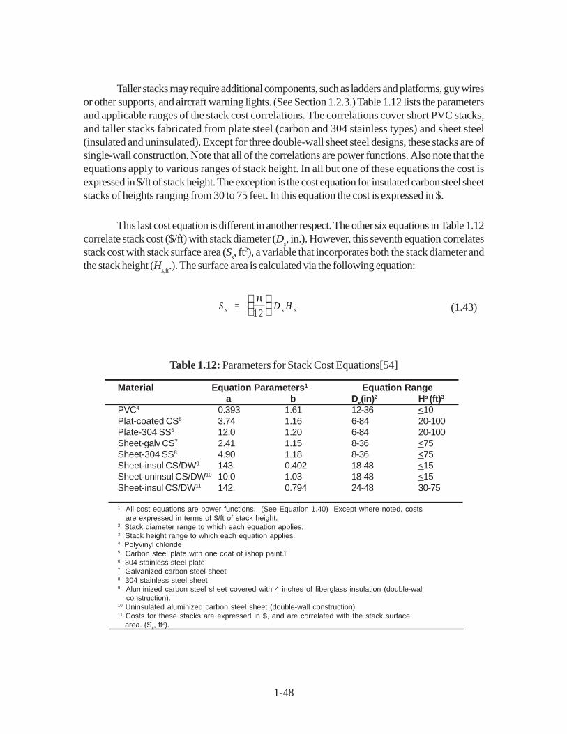
1-48

Taller stacks may require additional components, such as ladders and platforms, guy wiresor other supports, and aircraft warning lights. (See Section 1.2.3.) Table 1.12 lists the parametersand applicable ranges of the stack cost correlations. The correlations cover short PVC stacks,and taller stacks fabricated from plate steel (carbon and 304 stainless types) and sheet steel(insulated and uninsulated). Except for three double-wall sheet steel designs, these stacks are ofsingle-wall construction. Note that all of the correlations are power functions. Also note that theequations apply to various ranges of stack height. In all but one of these equations the cost isexpressed in $/ft of stack height. The exception is the cost equation for insulated carbon steel sheetstacks of heights ranging from 30 to 75 feet. In this equation the cost is expressed in $.

This last cost equation is different in another respect. The other six equations in Table 1.12correlate stack cost ($/ft) with stack diameter (D

s, in.). However, this seventh equation correlates

stack cost with stack surface area (Ss, ft2), a variable that incorporates both the stack diameter and

the stack height (Hs,ft

.). The surface area is calculated via the following equation:

S Hs s = D s

π1 2

(1.43)

Table 1.12: Parameters for Stack Cost Equations[54]

Material Equation Parameters1 Equation Range a b Ds(in)2 Hs (ft)3

PVC4 0.393 1.61 12-36 <10Plat-coated CS5 3.74 1.16 6-84 20-100Plate-304 SS6 12.0 1.20 6-84 20-100Sheet-galv CS7 2.41 1.15 8-36 <75Sheet-304 SS8 4.90 1.18 8-36 <75Sheet-insul CS/DW9 143. 0.402 18-48 <15Sheet-uninsul CS/DW10 10.0 1.03 18-48 <15Sheet-insul CS/DW11 142. 0.794 24-48 30-75

1 All cost equations are power functions. (See Equation 1.40) Except where noted, costs are expressed in terms of $/ft of stack height.2 Stack diameter range to which each equation applies.3 Stack height range to which each equation applies.4 Polyvinyl chloride5 Carbon steel plate with one coat of ìshop paint.î6 304 stainless steel plate7 Galvanized carbon steel sheet8 304 stainless steel sheet9 Aluminized carbon steel sheet covered with 4 inches of fiberglass insulation (double-wall construction).10 Uninsulated aluminized carbon steel sheet (double-wall construction).11 Costs for these stacks are expressed in $, and are correlated with the stack surface area. (Ss, ft

2).

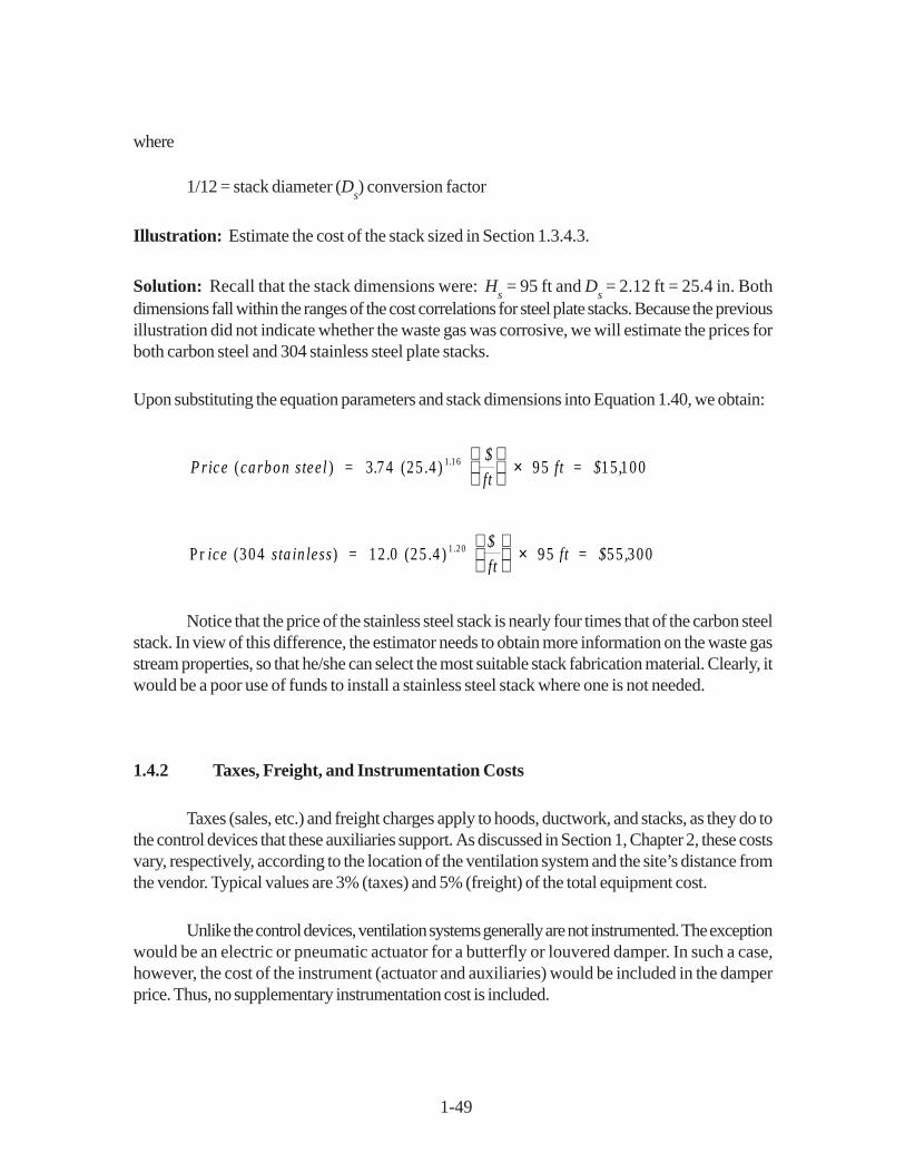
1-49

where

1/12 = stack diameter (Ds) conversion factor

Illustration: Estimate the cost of the stack sized in Section 1.3.4.3.

Solution: Recall that the stack dimensions were: Hs = 95 ft and D

s = 2.12 ft = 25.4 in. Both

dimensions fall within the ranges of the cost correlations for steel plate stacks. Because the previousillustration did not indicate whether the waste gas was corrosive, we will estimate the prices forboth carbon steel and 304 stainless steel plate stacks.

Upon substituting the equation parameters and stack dimensions into Equation 1.40, we obtain:

P rice = ft = $( ) (25 .4 ) .carbon stee l . $

ft ,3 74 95 15 1001 16

×

P r (304 ) (25 .4 ) 1.20ice .$

ft, s ta in less = ft = $12 0 95 55 300

×

Notice that the price of the stainless steel stack is nearly four times that of the carbon steelstack. In view of this difference, the estimator needs to obtain more information on the waste gasstream properties, so that he/she can select the most suitable stack fabrication material. Clearly, itwould be a poor use of funds to install a stainless steel stack where one is not needed.

1.4.2 Taxes, Freight, and Instrumentation Costs

Taxes (sales, etc.) and freight charges apply to hoods, ductwork, and stacks, as they do tothe control devices that these auxiliaries support. As discussed in Section 1, Chapter 2, these costsvary, respectively, according to the location of the ventilation system and the site’s distance fromthe vendor. Typical values are 3% (taxes) and 5% (freight) of the total equipment cost.

Unlike the control devices, ventilation systems generally are not instrumented. The exceptionwould be an electric or pneumatic actuator for a butterfly or louvered damper. In such a case,however, the cost of the instrument (actuator and auxiliaries) would be included in the damperprice. Thus, no supplementary instrumentation cost is included.

1-50

1.4.3 Purchased Equipment Cost

With ventilation systems, the purchased equipment cost (PECt) is the sum of the equipment,

taxes, and freight costs. Incorporating the typical values listed in Section 1.4.2, we obtain:

P E C = E C + . E C + . E C = . t t t t 0 03 0 05 1 08 ( )E C t (1.44)

where

ECt = total cost of hood(s), ductwork, and stack(s)

1.4.4 Installation Costs

When making a cost estimate for an air pollution control system according to the procedurein this Manual, the estimator first determines the cost of the control device, then estimates the costsof such auxiliaries as the hood, ductwork, stack, fan and motor, and other items. To these items he/she adds the costs of instrumentation, taxes, and freight, to obtain the PEC. Finally, the estimatormultiplies the PEC by the installation factor appropriate to the control device (e.g., 2.20 for gasabsorbers) to obtain the total capital investment. In these cases, the installation factor incorporatesall direct and indirect costs needed to install and start up the control system equipment, including,of course, the hood, ductwork, and stack.

For this reason, it usually is unnecessary to estimate the installation cost of the ventilationsystem separately. However, there may be occasions where a hood, a stack, or ductwork has tobe installed alone, either as replacement equipment or to augment the existing ventilation system. Inthose instances, the estimator may want to estimate the cost of installing this item.

As might be imagined, these installation costs vary considerably, according to geographiclocation, size and layout of the facility, equipment design, and sundry other variables. Nonetheless,some of the vendors (and a peer reviewer[59]) provided factors for hoods and ductwork, which,when multiplied by their respective purchased equipment costs, will yield approximate installationcosts. These are:

• Hoods: 50 to 100%

• Ductwork: 25 to 50%

If one or both of these factors is used, the total capital investment (TCI) of the hood and/orductwork would be:

T C I + IF h/d= P E C h / d( )1 × (1.45)where

IFh/d

= installation factor for hood(h)/ductwork(d)

PECh/d

= purchased equipment cost of hood (h)/ductwork (d)

1-51

1.5 Estimating Total Annual Cost

1.5.1 Direct Annual Costs

Ventilation systems incur few, if any, direct annual costs, as they function to support controldevices. There are no costs for operating or supervisory labor, operating materials, or wastetreatment/disposal allocated to ventilation systems. Maintenance costs would also be minimal,except for such minor expenses as painting, insulation repair, or calibration of automatic dampercontrols. The only utilities cost would be the incremental electricity needed for the waste gasstream to overcome the static pressure loss in the hood, ducting, and stack.3 The incremental

electricity cost (Cc, $/yr) can be calculated as follows:

CQ F

cd =

p c(1 .175 10 )-4×∈

θ(1.46)

where

pc

= electricity price ($/kwh)

Q = waste gas flow rate (actual ft3/min)

F = static pressure drop through ventilation system (in. w.c.)� = operating factor (hr/yr)� = combined fan-motor efficiency

Illustration: In the cosmetic factory ventilation system, what would be the cost of the electricityconsumed by the fan needed to convey the gas through the ductwork? Assume an electricity priceof $0.075/kwh, a combined fan-motor efficiency of 0.6, and an 8,000-hr/yr operating factor.

Solution: Recall that the pressure drop and gas flow rate for this illustration were 0.313 in. w.c.and 15,000 actual ft3/min, respectively. Upon substituting these values and the other parametersinto equation 10.40, we obtain:

Cc = (1.175 x 10-4) (0.075) (15,000) (0.313) (8,000)/0.6 = $552/yr.

1.5.2 Indirect Annual Costs

The indirect annual costs for ventilation systems include property taxes, insurance, generaland administrative (G&A), and capital recovery costs. (Overhead—a fifth indirect annual cost—is not considered, because it is factored from the sum of the operating, supervisory, maintenance

3 Technically, this direct annual cost should be allocated to the ventilation system fan, not to the hood, ductwork, and stack. The fan power cost equation will be included in the Manual section on fans. However, as the fans section has yet to be written, this equation has been provided as a temporary convenience to Manual users.

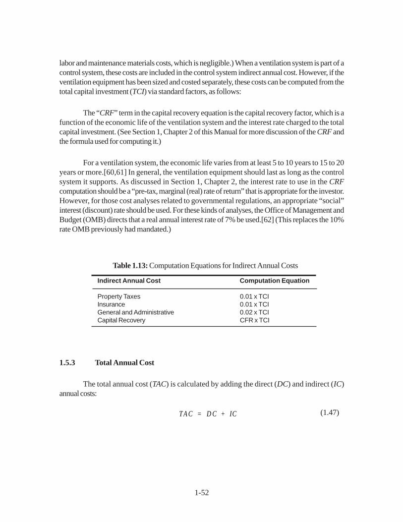
1-52

labor and maintenance materials costs, which is negligible.) When a ventilation system is part of acontrol system, these costs are included in the control system indirect annual cost. However, if theventilation equipment has been sized and costed separately, these costs can be computed from thetotal capital investment (TCI) via standard factors, as follows:

The “CRF” term in the capital recovery equation is the capital recovery factor, which is afunction of the economic life of the ventilation system and the interest rate charged to the totalcapital investment. (See Section 1, Chapter 2 of this Manual for more discussion of the CRF andthe formula used for computing it.)

For a ventilation system, the economic life varies from at least 5 to 10 years to 15 to 20years or more.[60,61] In general, the ventilation equipment should last as long as the controlsystem it supports. As discussed in Section 1, Chapter 2, the interest rate to use in the CRFcomputation should be a “pre-tax, marginal (real) rate of return” that is appropriate for the investor.However, for those cost analyses related to governmental regulations, an appropriate “social”interest (discount) rate should be used. For these kinds of analyses, the Office of Management andBudget (OMB) directs that a real annual interest rate of 7% be used.[62] (This replaces the 10%rate OMB previously had mandated.)

Table 1.13: Computation Equations for Indirect Annual Costs

Indirect Annual Cost Computation Equation

Property Taxes 0.01 x TCIInsurance 0.01 x TCIGeneral and Administrative 0.02 x TCICapital Recovery CFR x TCI

1.5.3 Total Annual Cost

The total annual cost (TAC) is calculated by adding the direct (DC) and indirect (IC)annual costs:

T A C = D C + IC (1.47)

1-53

1.6 Acknowledgements

Several firms and individuals provided very useful technical and cost information to thischapter. Foremost among these was Todd N. Stine of United McGill Corporation (Raleigh, NC),who submitted current prices for a variety of ductwork items, as well as a comprehensive productcatalog and engineering design manual. In addition, Mr. Stine patiently replied to the author’s manyquestions, providing supplemental data when requested. Samir Karandikar of EPCON IndustrialSystems (The Woodlands, TX) and Gregory P. Michaels of Piping Technology & Products(Houston, TX) also were very helpful in submitting data and responding to inquiries.

The author also would like to thank the following firms for their valuable contributions:

• Air Plastics, Inc. (Mason, OH)

• General Resource Corporation (Hopkins, MN)

• Harrington Industrial Plastics, Inc. (Chino, CA)

• Intellect Systems & Marketing, Inc. (Bohemia, NY)

• Wer-Coy Metal Fabrication Co. (Warren, MI)

In addition, several individuals reviewed the draft chapter and provided valuable suggestions,supplemental information, or both. The EPA peer reviewers, all located at Research Triangle Park,NC, were:

• James C. Berry (OAQPS/ESD)

• Peter A. Eckhoff (OAQPS/TSD)

• Norman Kaplan (ORD/AEERL)

• James H. Maysilles (OAQPS/ESD)

• Larry Sorrels (OAQPS/ESD)

Finally, Howard Goodfellow of Goodfellow Consultants, Inc. (Mississauga, Ontario,Canada) also reviewed this Section and supplied helpful comments.

1-54

References

[1] Goodfellow, H.D. “Ancillary Equipment for Local Exhaust Ventilation Systems”. In: AirPollution Engineering Manual. New York, NY: Van Nostrand Reinhold/Air and WasteManagement Association. 1992, pp. 155-205.

[2] Burton, D. Jeff. Industrial Ventilation Work Book. Salt Lake City: DJBA, Inc. 1989.

[3] The Measurement Solution: Using a Temporary Total Enclosure for Capture EfficiencyTesting. Research Triangle Park, NC: U.S. Environmental Protection Agency. August1991 (EPA-450/4-91-020), pp. 3,11.

[4] The Measurement Solution, pp. 11-29.

[5] Heinsohn, Robert Jennings. Industrial Ventilation: Engineering Principles. New York,NY: John Wiley & Sons, Inc. 1991.

[6] Telephone conversation between William M. Vatavuk, U.S. Environmental ProtectionAgency (Research Triangle Park, NC) and Todd N. Stine, United McGill Company(Raleigh, NC), May 24, 1993.

[7] Thermoplastic Duct (PVC) Construction Manual, 2nd Edition 1994. Vienna, VA: SheetMetal and Air Conditioning Contractors’ National Association, Inc. (SMACNA). May1987, pp. 61-85.

[8] Thermoplastic Duct Construction Manual, p. 64.

[9] Burton, p. 6-7.

[10] Dust Control System Accessories Price List. Huntington Park, CA: Murphy-Rodgers,Inc. July 1992.

[11] Price and Data Catalog: Standard Ductwork Components. Warren, MI: Wer-Coy MetalFabrication Co. 1992-93.

[12] Letters from Samir Karandikar, EPCON Industrial Systems (Woodlands, TX) to WilliamM. Vatavuk, U.S. Environmental Protection Agency (Research Triangle Park, NC). May21 and June 9, 1993.

[13] “Double Wall Insulated Duct and Fittings.” In: Sheet Metal Division Catalog. Groveport,OH: United McGill Corporation. 1990.

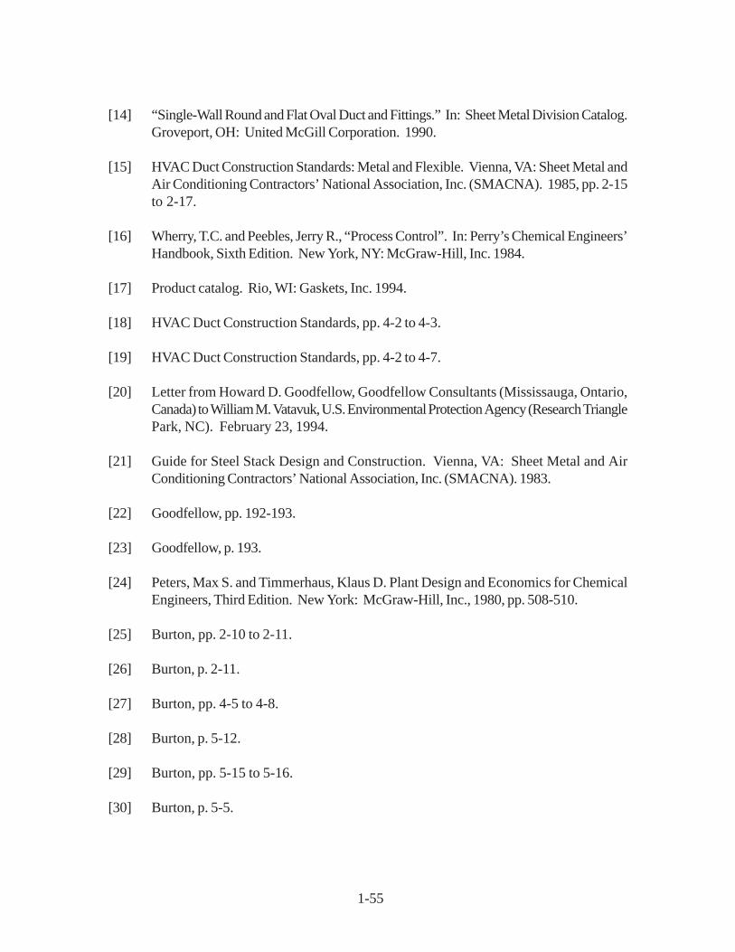
1-55

[14] “Single-Wall Round and Flat Oval Duct and Fittings.” In: Sheet Metal Division Catalog.Groveport, OH: United McGill Corporation. 1990.

[15] HVAC Duct Construction Standards: Metal and Flexible. Vienna, VA: Sheet Metal andAir Conditioning Contractors’ National Association, Inc. (SMACNA). 1985, pp. 2-15to 2-17.

[16] Wherry, T.C. and Peebles, Jerry R., “Process Control”. In: Perry’s Chemical Engineers’Handbook, Sixth Edition. New York, NY: McGraw-Hill, Inc. 1984.

[17] Product catalog. Rio, WI: Gaskets, Inc. 1994.

[18] HVAC Duct Construction Standards, pp. 4-2 to 4-3.

[19] HVAC Duct Construction Standards, pp. 4-2 to 4-7.

[20] Letter from Howard D. Goodfellow, Goodfellow Consultants (Mississauga, Ontario,Canada) to William M. Vatavuk, U.S. Environmental Protection Agency (Research TrianglePark, NC). February 23, 1994.

[21] Guide for Steel Stack Design and Construction. Vienna, VA: Sheet Metal and AirConditioning Contractors’ National Association, Inc. (SMACNA). 1983.

[22] Goodfellow, pp. 192-193.

[23] Goodfellow, p. 193.

[24] Peters, Max S. and Timmerhaus, Klaus D. Plant Design and Economics for ChemicalEngineers, Third Edition. New York: McGraw-Hill, Inc., 1980, pp. 508-510.

[25] Burton, pp. 2-10 to 2-11.

[26] Burton, p. 2-11.

[27] Burton, pp. 4-5 to 4-8.

[28] Burton, p. 5-12.

[29] Burton, pp. 5-15 to 5-16.

[30] Burton, p. 5-5.

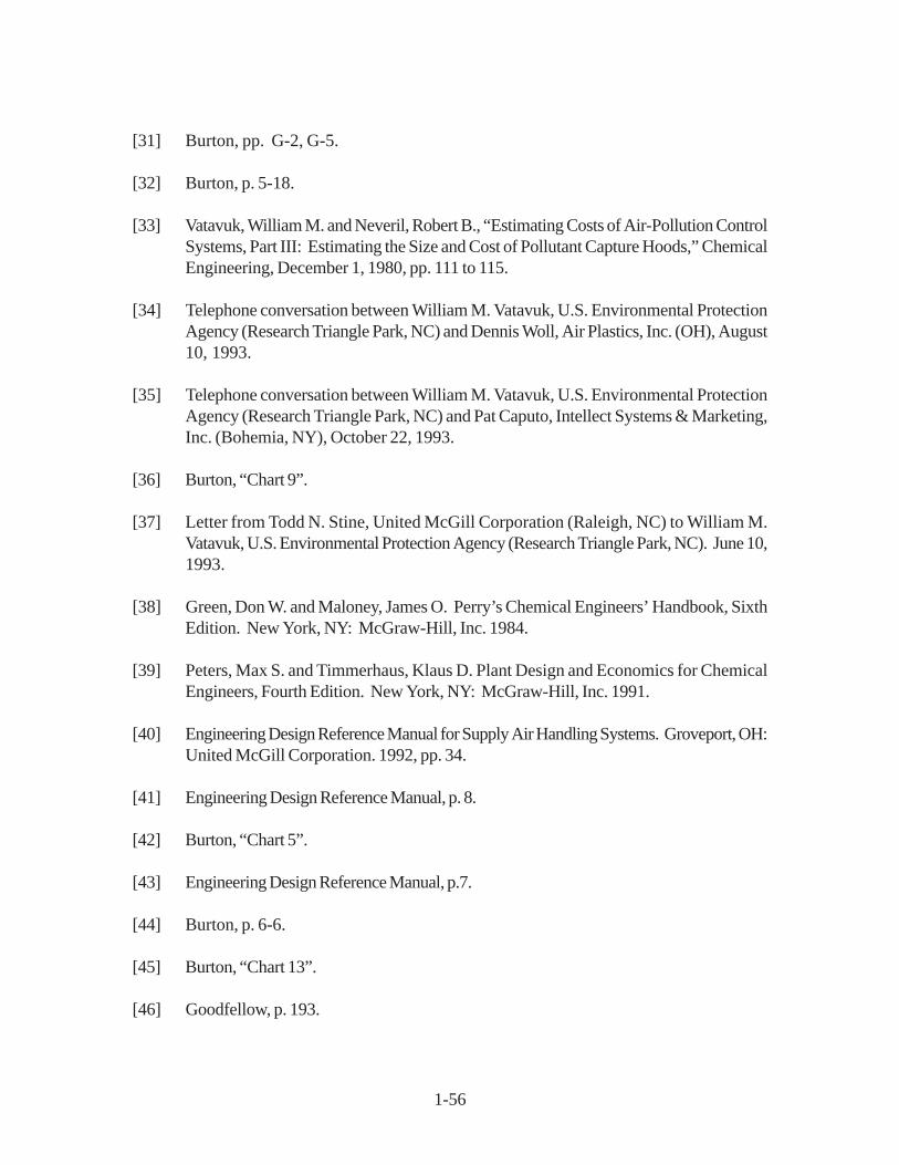
1-56

[31] Burton, pp. G-2, G-5.

[32] Burton, p. 5-18.

[33] Vatavuk, William M. and Neveril, Robert B., “Estimating Costs of Air-Pollution ControlSystems, Part III: Estimating the Size and Cost of Pollutant Capture Hoods,” ChemicalEngineering, December 1, 1980, pp. 111 to 115.

[34] Telephone conversation between William M. Vatavuk, U.S. Environmental ProtectionAgency (Research Triangle Park, NC) and Dennis Woll, Air Plastics, Inc. (OH), August10, 1993.

[35] Telephone conversation between William M. Vatavuk, U.S. Environmental ProtectionAgency (Research Triangle Park, NC) and Pat Caputo, Intellect Systems & Marketing,Inc. (Bohemia, NY), October 22, 1993.

[36] Burton, “Chart 9”.

[37] Letter from Todd N. Stine, United McGill Corporation (Raleigh, NC) to William M.Vatavuk, U.S. Environmental Protection Agency (Research Triangle Park, NC). June 10,1993.

[38] Green, Don W. and Maloney, James O. Perry’s Chemical Engineers’ Handbook, SixthEdition. New York, NY: McGraw-Hill, Inc. 1984.

[39] Peters, Max S. and Timmerhaus, Klaus D. Plant Design and Economics for ChemicalEngineers, Fourth Edition. New York, NY: McGraw-Hill, Inc. 1991.

[40] Engineering Design Reference Manual for Supply Air Handling Systems. Groveport, OH:United McGill Corporation. 1992, pp. 34.

[41] Engineering Design Reference Manual, p. 8.

[42] Burton, “Chart 5”.

[43] Engineering Design Reference Manual, p.7.

[44] Burton, p. 6-6.

[45] Burton, “Chart 13”.

[46] Goodfellow, p. 193.

1-57

[47] Guide for Steel Stack Design and Construction, pp. 39 to 50.

[48] Goodfellow, p. 193.

[49] Carlton-Jones, Dennis and Schneider, H.B., “Tall Chimneys,” Chemical Engineering,October 14, 1968, p. 167.

[50] Guideline for Determination of Good Engineering Practice: Stack Height (Technical SupportDocument for Stack Height Regulations) (Revised). Research Triangle Park, NC: U.S.Environmental Protection Agency. June 1985 (NTIS PB-85-225241), p.1.

[51] Guideline for Determination of Good Engineering Practice, pp. 50-51.

[52] Guideline for Determination of Good Engineering Practice, pp. 1-2.

[53] Goodfellow, p. 194.

[54] Guide for Steel Stack Design and Construction, p. 4.

[55] Hood cost data request responses from four hood vendors to William M. Vatavuk, U.S.Environmental Protection Agency (Research Triangle Park, NC). June-July 1993.

[56] Ductwork cost data request responses from six vendors to William M. Vatavuk, U.S.Environmental Protection Agency (Research Triangle Park, NC). May-July 1993.

[57] Stack cost data request responses from four vendors to William M. Vatavuk, U.S.Environmental Protection Agency (Research Triangle Park, NC). May-July 1993.

[58] Op. cit., Stine-Vatavuk letter, June 10, 1993.

[59] Goodfellow-Vatavuk letter.

[60] Goodfellow-Vatavuk letter.

[61] Telephone conversation between William M. Vatavuk, U.S. Environmental ProtectionAgency (Research Triangle Park, NC) and Todd N. Stine, United McGill Company(Raleigh, NC), December 10, 1993.

[62] Darman, Richard. Guidelines and Discount Rates for Benefit-Cost Analysis of FederalPrograms (OMB Circular No. A-94 Revised). Washington, DC: Office of Managementand Budget. October 29, 1992.

TECHNICAL REPORT DATA(Please read Instructions on reverse before completing)

1. REPORT NO.

452/B-02-0012. 3. RECIPIENT'S ACCESSION NO.

4. TITLE AND SUBTITLE

The EPA Air Pollution Control Cost Manual

5. REPORT DATE

January, 2002 6. PERFORMING ORGANIZATION CODE

7. AUTHOR(S)

Daniel Charles Mussatti

8. PERFORMING ORGANIZATION REPORT NO.

9. PERFORMING ORGANIZATION NAME AND ADDRESS

U.S. Environmental Protection Agency Office of Air Quality Planning and Standards Air Quality Standards and Strategies Division Innovative Strategies and Economics Group Research Triangle Park, NC 27711

10. PROGRAM ELEMENT NO.

11. CONTRACT/GRANT NO.

12. SPONSORING AGENCY NAME AND ADDRESS

Director Office of Air Quality Planning and Standards Office of Air and Radiation U.S. Environmental Protection Agency Research Triangle Park, NC 27711

13. TYPE OF REPORT AND PERIOD COVERED

Final

14. SPONSORING AGENCY CODE

EPA/200/04

15. SUPPLEMENTARY NOTES

Updates and revises EPA 453/b-96-001, OAQPS Control Cost Manual, fifth edition (in English only)

16. ABSTRACT

In Spanish, this document provides a detailed methodology for the proper sizing and costing of numerous airpollution control devices for planning and permitting purposes. Includes costing for volatile organiccompounds (VOCs); particulate matter (PM); oxides of nitrogen (NOx); SO2, SO3, and other acid gasses;and hazardous air pollutants (HAPs).

17. KEY WORDS AND DOCUMENT ANALYSIS

a. DESCRIPTORS b. IDENTIFIERS/OPEN ENDED TERMS c. COSATI Field/Group

EconomicsCostEngineering costSizingEstimationDesign

Air Pollution controlIncineratorsAbsorbersAdsorbersFiltersCondensersElectrostatic PrecipitatorsScrubbers

18. DISTRIBUTION STATEMENT

Release Unlimited

19. SECURITY CLASS (Report)

Unclassified21. NO. OF PAGES

1,400

20. SECURITY CLASS (Page)

Unclassified22. PRICE

EPA Form 2220-1 (Rev. 4-77)EPA Form 2220-1 (Rev. 4-77) PREVIOUS EDITION IS OBSOLETE