SECTION 11.2Carrying Out Significance Tests

Steps for Significance Testing

1)Hypothesis

2)Conditions

3)Calculations

4)Interpretation

Step 1: Hypothesis•Identify the population of interest and the parameter you want to draw conclusions about.

•State the hypothesis

•Is the mean of the population equal to, less than, or greater than a specific value?

Step 2: Conditions•Choose the appropriate inference procedure

•Population mean or population proportion?

1) SRS2) Normality3) Independence

Step 3: Calculations•If the conditions are met, carry out the inference procedure.

•If conditions aren’t met, make note of the issue and continue with the problem.

•1. Calculate the test statistic.

•2. Find the P-value

z Test for a Population Mean• To test the Hypothesis 𝐻0: 𝜇 = 𝜇0 based on an SRS of size n from

a population with unknown mean, 𝜇, and known standard deviation, 𝜎, compute the one-sample z statistic:

𝑧 = 𝑥 − 𝜇0

𝜎

𝑛

• In terms of a variable Z having the standard Normal distribution, the P-value for a test of 𝐻0 against:

•𝐻𝑎: 𝜇 > 𝜇0 is 𝑃 𝑍 ≥ 𝑧

•𝐻𝑎: 𝜇 < 𝜇0 is 𝑃 𝑍 ≤ 𝑧

•𝐻𝑎: 𝜇 ≠ 𝜇0 is 𝑃 𝑍 ≥ 𝑧•𝑃 𝑍 ≥ 𝑧 and 𝑃 𝑍 ≤ −𝑧

• These P-values are exact if the population distribution is Normal and are approximately correct for large n in other cases.

Example: Blood Pressure• The medical director of a large company is concerned about the

effects of stress on the company’s younger executives. According to the National Center for Health Statistics, the mean systolic blood pressure for males 35 to 44 years of age is 128, and the standard deviation in this population is 15.

• The medical director examines the medical records of 72 male executives in this age group and finds their mean systolic blood pressure is 𝑥 = 129.93

• Is this evidence that the mean blood pressure for all the company’s younger male executives is different from the National Average?

Step 1: Hypothesis• The population of interest is all middle-aged male executives in

this company.

•𝐻0 and 𝐻𝑎?•𝐻0: 𝜇 = 128 Younger male company executives’ mean blood

pressure is 128.

•𝐻𝑎: 𝜇 ≠ 128 Younger male executives’ mean blood pressure differs from the national mean of 128.

• This is a two-sided or two-tailed test.

Step 2: Conditions• SRS: We are not told that this is an SRS. If the sample was taken

with some other method our results may not be appropriate.

• Normality: We do not know that the population distribution of blood pressures among the company executives is Normally distributed. But, the large sample size tells us that the sampling distribution of 𝑥 will be approximately Normal (by the Central Limit Theorem)

• Independence: Since the medical director is selecting executives without replacement, we must assume that there is at least (10)(72) = 720 middle aged male executives in this large company.

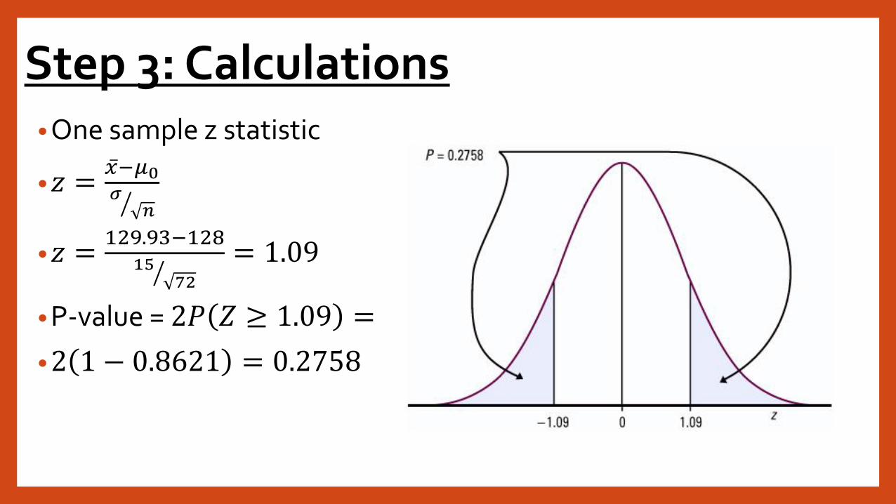
Step 3: Calculations• One sample z statistic

•𝑧 = 𝑥−𝜇0

𝜎

𝑛

•𝑧 =129.93−128

1572

= 1.09

• P-value = 2𝑃 𝑍 ≥ 1.09 =

•2 1 − 0.8621 = 0.2758

Step 4: Interpretation• More than 27% of the time, an SRS of size 72 from the general population

would have a mean blood pressure at least as far from 128 as that of the executive sample.

• The observed 𝑥 = 129.93 is therefore not good evidence that middle-aged male executives’ blood pressures differ from the national average.

• We fail to reject 𝐻0

• This doesn’t mean that the blood pressure for middle aged executives is 128.

• We sought to show that 𝜇 differed from 128 and failed to find convincing evidence.

Example: Health Promotion Program• The company medical director from the last example institutes a

health promotion campaign to encourage employees to exercise more and eat a healthier diet.

• The director chooses a random sample of 50 employees and compares their blood pressures from physical exams given before the campaign and again a year later.

• The mean change in systolic blood pressure for these n = 50 employees is 𝑥 = −6. We take the population standard deviation to be 𝜎 = 20.

• The director decides to use an 𝛼 = 0.05 significance level.

Step 1: Hypothesis• We want to know if the health campaign reduced blood

pressure on average in the population of all employees at this large company. Taking 𝜇 to be the mean change in blood pressure for all employees, we test:

•𝐻0: 𝜇 = 0

•𝐻𝑎: 𝜇 < 0

Step 2: Conditions• Since 𝜎 is known, we will use a one-sample z test for a population mean.

• SRS: The medical director took a “random sample” of 50 company employees. We have to assume this was an SRS. If a different method was used our results may not be appropriate.

• Normality: The large sample size (𝑛 = 50) lets us assume approximate Normality of the sampling distribution of 𝑥, even if the population distribution of change in blood pressure isn’t Normal.

• Independence: There must be at least (10)(50) = 500 employees in this large company since the medical director is sampling without replacement.

Step 3: Calculations• Test Statistic: One sample z-test

• 𝑧 = 𝑥−𝜇0

𝜎

𝑛

• 𝑧 =−6−0

2050

= −2.12

• P-value: Because 𝐻𝑎 is one-sided on the low side, large negative values of z count against 𝐻0. The P-value is:

•𝑃 = 𝑃 𝑍 ≤ −2.12 = 0.0170

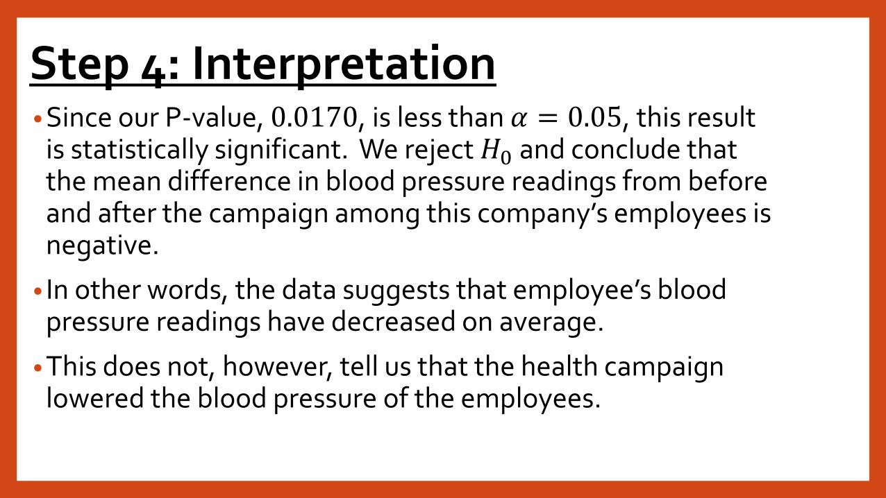
Step 4: Interpretation• Since our P-value, 0.0170, is less than 𝛼 = 0.05, this result

is statistically significant. We reject 𝐻0 and conclude that the mean difference in blood pressure readings from before and after the campaign among this company’s employees is negative.

• In other words, the data suggests that employee’s blood pressure readings have decreased on average.

• This does not, however, tell us that the health campaign lowered the blood pressure of the employees.

Tests from Confidence Intervals• Confidence intervals and significance tests are closely related.

• If we have a 95% confidence interval, then we are 95% confident that our true mean, 𝜇, lies inside our interval. We are also confident that values of 𝜇that fall outside our interval are incompatible with our data.

• This outer 5% is what makes up our two-tailed 𝛼 = 0.05 significance level.

• A level 𝛼 two-sided significance test rejects a hypothesis 𝐻0: 𝜇 = 𝜇0exactly when the value 𝜇0 falls outside a level 1 − 𝛼 confidence interval for 𝜇.

• This is sometimes called duality.

Example: Analyzing Drugs• A laboratory analyzes specimens of a drug to determine the concentration

of the active ingredient. Such chemical analyses are not perfectly precise.

• Repeated measurements on the same specimen will give slightly different results. The results of repeated measurements follow a Normal distribution. The analysis procedure has no bias, so the mean, 𝜇, of the population of all measurements is the true concentration of the specimen.

• The standard deviation of this distribution is a property of the analysis method and is known to be 𝜎 = 0.0068 grams per liter. The laboratory analyzes each specimen three times and reports the mean result.

Example: Analyzing drugs (cont.)• A client sends a specimen for which the concentration of active

ingredients is supposed to be 0.86%. The laboratory’s analysis gives the following 3 concentrations:

𝟎. 𝟖𝟒𝟎𝟑 𝟎. 𝟖𝟑𝟔𝟑 𝟎. 𝟖𝟒𝟒𝟕

• Is there significant evidence at the 1% level that the true concentration is not 0.86%?

Step 1: Hypothesis•The population is all possible measurements of the specimen.

•The parameter is the mean concentration.

•𝐻0: 𝜇 = 0.86

•𝐻𝑎: 𝜇 ≠ 0.86

Step 2: Conditions•SRS: This is not an SRS, so our conclusion may not be

appropriate.

•Normality: We are told that the repeated measurements follow a Normal distribution.

•Independence: The readings should be independent.

Step 3: Calculations• 𝑥 = 0.8404

• A one-sample z-test is appropriate:

•𝑧 = −4.99

• This z score is not on our Table A. The largest negative value on Table A is −3.49. All we can say from Table A is that 𝑧 ≤ −3.49

• P-value: 2𝑃 𝑍 ≤ −3.49 = 2 1 − 0.9998 = 0.0004

• This is less than the 𝛼 = 0.01, so we can reject 𝐻0.

Step 4: Interpretation•Since our P-value is so low, we can reject 𝐻0

•We can conclude that the concentration of the specimen is not 0.86

Confidence Interval•Create a 99% confidence interval for 𝜇, the concentration of the sample.

Step 1: Parameter•Population: All possible measurements of the specimen.

•Parameter: Mean concentration.

Step 2: Conditions

• SRS: This is not an SRS, so our conclusion may not be appropriate.

• Normality: We are told that the repeated measurements follow a Normal distribution.

• Independence: The readings should be independent.

Step 3: Calculation•99% Confidence Interval

𝑥 ± 𝑧∗𝜎

𝑛

0.8404 ± 2.5750.0068

3

0.8404 ± 0.0101

0.8303, 0.8505

Step 4: Interpretation• We are 99% confident that the true mean concentration of

the specimen is between 0.8303 and 0.8505.

Connection• After performing an 𝛼 = 0.01 level significance test, we found that

we could reject 𝐻0: 𝜇 = 0.86

• This led us to the conclusion that the true mean concentration was not 0.86.

• When we did a 99% confidence interval we determined that we were 99% confident that the true mean concentration was between 0.8303 and 0.8505, which does not include 0.86.

• These 2 procedures are different ways of looking at the same thing.

• This will only work for a two-sided significance test.

Connection (cont.)• If the 𝐻0 is included in a 1 − 𝛼 confidence interval, then we will fail to

reject 𝐻0 in an 𝛼 level significance test

• If the 𝐻0 is NOT included in a 1 − 𝛼 confidence interval, then we will reject 𝐻0 in an 𝛼 level significance test

• If 𝛼 = 0.05, then 1 − 𝛼 = 0.95

• If 𝛼 = 0.01, then 1 − 𝛼 = 0.99