Secondary effects in neural network analysis of the

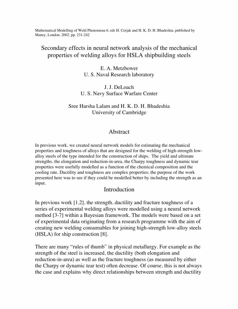
Mathematical Modelling of Weld Phenomena 6, eds H. Cerjak and H. K. D. H. Bhadeshia, published byManey, London, 2002. pp. 231-242

Secondary effects in neural network analysis of the mechanicalproperties of welding alloys for HSLA shipbuilding steels

E. A. MetzbowerU. S. Naval Research laboratory

J. J. DeLoachU. S. Navy Surface Warfare Center

Sree Harsha Lalam and H. K. D. H. BhadeshiaUniversity of Cambridge

Abstract

In previous work, we created neural network models for estimating the mechanicalproperties and toughness of alloys that are designed for the welding of high-strength low-alloy steels of the type intended for the construction of ships. The yield and ultimatestrengths, the elongation and reduction-in-area, the Charpy toughness and dynamic tearproperties were usefully modelled as a function of the chemical composition and thecooling rate. Ductility and toughness are complex properties; the purpose of the workpresented here was to see if they could be modelled better by including the strength as aninput.

Introduction

In previous work [1,2], the strength, ductility and fracture toughness of aseries of experimental welding alloys were modelled using a neural networkmethod [3-7] within a Bayesian framework. The models were based on a setof experimental data originating from a research programme with the aim ofcreating new welding consumables for joining high-strength low-alloy steels(HSLA) for ship construction [8].

There are many “rules of thumb” in physical metallurgy. For example as thestrength of the steel is increased, the ductility (both elongation andreduction-in-area) as well as the fracture toughness (as measured by eitherthe Charpy or dynamic tear test) often decrease. Of course, this is not alwaysthe case and explains why direct relationships between strength and ductility

or toughness are rare. It is for this reason that we decided to utilize theneural network method to determine if better predictions of the ductility andfracture toughness could be made if either the yield or ultimate strength wasincluded as an input variable along with the chemical composition and thecooling rate.

Data Base

The set of experimental data is summarised in Table 1 [1,2]. Theindependent variables are the chemical composition of the as-deposited weldmetal, the cooling rate at 538˚C, the measured yield or ultimate strength.The dependent variables are the elongation, reduction-in-area, the measuredCharpy V-notch values at –18 or –51˚C, or the dynamic tear test values at –1or –29˚C. The cooling rate was determined from the welding parameters(voltage, current, welding speed), preheat, and thickness of the plate [9,10].Table 1 gives the minimum, maximum, mean, and standard deviation eachof the variables.

The dynamic tear test results are generated on welds which did not containtitanium. A detailed description of both the data set and the neural networkemployed is found in the prior study [1,2].

One aspect of avoiding over fitting in the development of a neural networkrequires that the data set be divided into a training and a test set. There arealso other features described in [3-7] that implement automatic relevancedetermination. The model is at first produced using only the training dataset. It is then used to see how it generalises on the unseen test data. Bymonitoring both the training and test errors, it is possible to select the singlebest model.

It is, however, possible that a committee of models can make a more reliableprediction than an individual model [6-7]. To do this, the best models areranked using the values of the test errors. Committees are then formed bycombining the predictions of the best L models, where L = 1, 2, …… Thesize of the committee is given by the value of L. A plot of the test error ofthe committee versus its size L gives a minimum which defines the optimumsize of the committee.

Table 1: The input and output variables. The concentrations are in wt% except for oxygenand nitrogen which are in parts per million by weight. The cooling rate is expressed in°C/s.

Variable Minimum Maximum Mean Std. Dev. C 0.001 0.06 0.0307 0.0098 Mn 1.05 3.44 1.4361 0.1915

Si 0.05 0.4 0.2618 0.0555 Cr 0 0.21 0.0664 0.0530 Ni 1.66 5.63 3.1324 0.7800 Mo 0 1.23 0.5048 0.1452 Cu 0 0.48 0.1018 0.0766 S 0.001 0.012 0.0034 0.0019

P 0.001 0.015 0.0041 0.0026 Al 0.001 0.082 0.0066 0.0060 Ti 0.0008 0.3 0.0089 0.0181 Nb 0 0.069 0.0016 0.0041 V 0 0.031 0.0032 0.0042 B 0 0.01 0.0011 0.0021

O 109 627 216.7565 58.6969 N 6 135 29.8164 25.2642Cooling rate, ˚C/s 1.32 76.17 27.1079 23.0104YS, MPa 482 910 672.935 102.658UTS, MPa 589 971 742.708 86.503Elongation, % 3.5 29.2 20.8411 5.2370

Reduction-in-Area, %

7 84 94.6325 17.9575

CVN@-18˚C, J 8 358 181.9955 57.0641

CVN@-51˚C, J 3.8 242 143.6876 64.3903

DT@-1˚C, J 128 2606 1322.4916 538.1394

DT@-29˚C, J 80 2380 950.2694 583.3663

For each property, therefore, a committee of models was used to makepredictions. Once the optimum committee is selected, it was retrained on theentire data set without changing the complexity of each model, with theexception of the inevitable, although relatively small, adjustments to theweights. Normally the error bars that are plotted represent the fitting error,the magnitude of which depends on the position in the input space. Theadditional error sn is not usually plotted, but it is constant and can be takenas the highest value of sn for any member of the committee of models, aslisted in Table 2.

Table 2: The number of models in each committee, and the corresponding largest valueof sn.

Property Models sn

UTS 6 0.061YSUTS 14 0.047EL 9 0.128YSEL 8 0.127UTSEL 18 0.130RA 25 0.139YSRA 4 0.117UTSRA 19 0.140CVN@-18˚C 1 0.055YS CVN@-18˚C 80 0.109UTS CVN@-18˚C 7 0.063CVN@-51˚C 6 0.081YS CVN@-51˚C 2 0.081UTS CVN@-51˚C 11 0.080DT@-1˚C 6 0.091YS DT@-1˚C 2 0.098UTS DT@-1˚C 10 0.233DT@-29˚C 77 0.222YSDT@-29˚C 3 0.136UTSDT@-29˚C 6 0.139

Results and Discussion

Ultimate StrengthThe ultimate tensile strength was predicted by adding the yield strength tothe input variables. The data set consisted of 188 points. The results areshown in Fig, 1, where Fig.1a represents the predictions based oncomposition and cooling rate, and Fig. 1b is the predictions based oncomposition, cooling rate and yield strength. As might be expected, a bettercorrelation is obtained when the yield strength is added as a dependentvariable. It is useful to understand the significance of each input in

influencing the UTS. The significance sw, which is plotted in Fig. 1c, is ameasure to the extent to which an input variable can be correlated withvariations in the output. In that sense it is rather similar to a partialcorrelation coefficient in linear regression analysis. It is therefore worthemphasizing that whereas sw gives an indication of the correlation, it doesnot imply how sensitive the output is to the input – that information is in theweights. It is evident from Fig. 1c that the yield strength is an importantparameter determining the UTS.

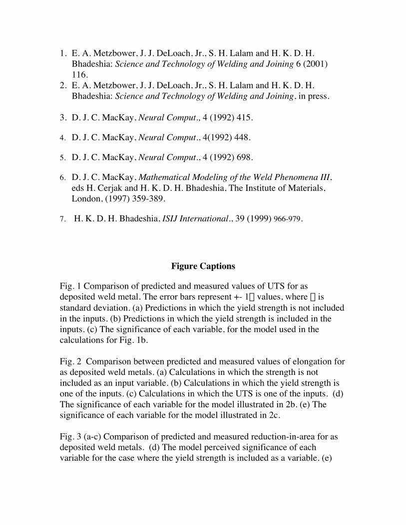
ElongationThere are three cases to consider: Fig. 2a is based on composition andcooling rate only; Fig. 2b is based on composition, cooling rate, and yieldstrength; Fig. 2c is based on composition, cooling rate, and ultimate strength.The number of data is 188 in all cases and the number of models in thecommittee is 9 in Fig 2a, and 8 for Fig. 2b and 18 for Fig. 2c.

The addition of the yield strength improves the predictability of theelongation (Fig. 2b), consistent with the observation in Fig. 2d that the yieldstrength is recognised to be a significant variable. On the other hand, theaddition of the ultimate strength degrades the predictions. A possible reasonwhy the inclusion of UTS does not help improve the estimation ofelongation is that much of the elongation consists of uniform strain, whereasthe ultimate tensile strength manifests at a point where necking begins. Thisis also seen in Fig. 2e, where the model perceived significance (sw ) of theUTS is seen to be negligible.

Reduction-in-AreaThe reduction of area has also been modelled in three ways: Fig. 3a is basedon composition and cooling rate only; Fig. 3b is based on composition,cooling rate, and yield strength; Fig. 3c is based on composition, coolingrate, and ultimate strength. The number of data is 160 in all cases and thenumber of models in the committee is 25 in Fig 3a, and 4 for Fig. 3b and 19for Fig. 3c. The addition of the yield or ultimate strength does not improvethe predictability of the reduction of area. This is also reflected in the largervalues of sn listed in Table 2.

An examination of the significance, sw (Figs. 3d,e), shows that consistentwith these observations, the oxide forming elements, aluminum and oxygen,are important in determining the reduction of area.

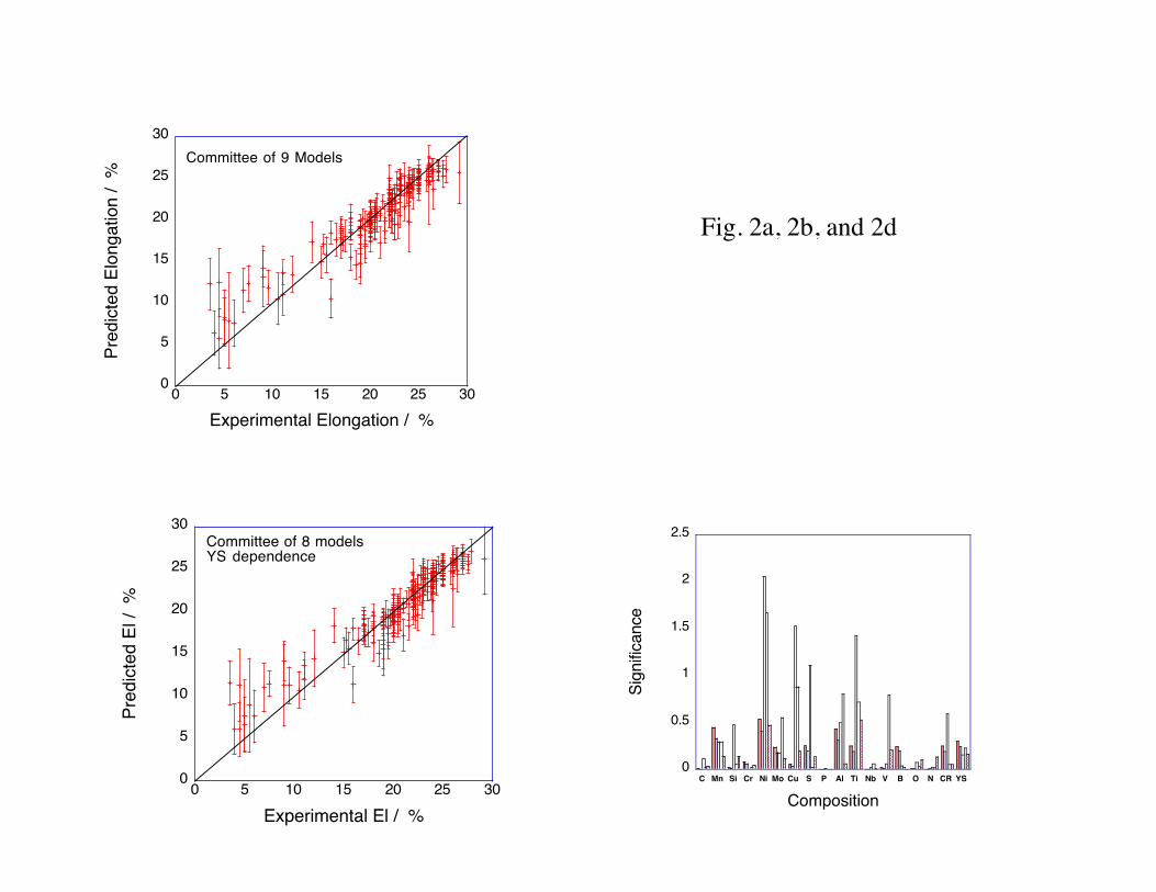
Charpy V-Notch TestsCVN@-18˚CFig. 4 depicts the predictions of the neural network for the case of theCharpy V-Notch tests at –18˚C. Fig. 4a is the original result, whereas Fig.4b includes the yield strength as input, and Fig. 4c includes the ultimatestrength. The original predictions are based on a data set of 602 points and acommittee of 1 model. The addition of the yield strength resulted in a dataset of 566 points and a committee of 80 models and the addition of theultimate strength resulted in a data set of 568 points and a committee of 7models.

CVN@-51˚CFig. 5 demonstrates the predictions of the neural network for the case of theCharpy V-Notch tests at –51˚C. Fig. 5a, which shows the original results,was determined using a committee of 6 models based on 602 points. Fig,5b, with the yield strength as input, has a data set of 584 points and acommittee of 2 models. Fig. 5c, ultimate strength as input, is based on adata set of 584 points and a committee of 11 models yielded the leastcorrelation.

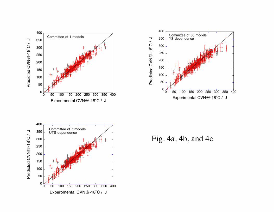
Dynamic Tear TestsDT@-1˚CFig. 6a discloses the predictions of the neural network for the case of thedynamic tear test at –1˚C for a data set of 180 points and a committee of 6models. The addition of the yield strength as a variable results in a data setof 180 points and a committee of 2 models. Substituting the ultimatestrength for the yield strength reduces the data set to 98 points and thecommittee of models becomes 10. The best correlation appears to be basedon chemistry and cooling rate only.

DT@-29˚CFig 7 shows the predictions of the neural network for the dynamic tear testsat –29˚C. The data set for all three cases was 180 points. Fig. 7a, the

original results, has a committee of 77 models. The addition of the yieldstrength increases the number of models in the committee to 3, whereas theaddition of the ultimate strength increases the number of models in thecommittee to 6. The addition of either yield or ultimate strength does notimprove the predictability of the dynamic tear tests at –29˚C.

Use of the Models in Predictions

The performance of the models can be used to make predictions regardingtrends as a function of each of the inputs. This is relatively straight forwardfor the calculation of the strength, ductility, and impact resistance as afunction of composition and cooling rate. The addition of strength as adependent variable complicates the predictive capability since it requiresfirst calculating either the yield or ultimate strength and then calculating thedesired property with the additional strength variable.

Summary

It is found that in most cases, the complex mechanical properties of a weldmetal are best represented in terms of the chemical composition and coolingrate alone.

The inclusion of the yield or ultimate strength as inputs failed to improve thepredictability of the neural network models, and did not provide any newinsight into trends as a function of the inputs. Furthermore, the modelsbecome more difficult to use since a knowledge of the strength is requiredbefore a calculation can be conducted.

Acknowledgements

Funding support from the Office of Naval Research (Arlington, VA USA),and from the Cambridge Commonwealth Trust, is gratefully acknowledged.

References

1. E. A. Metzbower, J. J. DeLoach, Jr., S. H. Lalam and H. K. D. H.Bhadeshia: Science and Technology of Welding and Joining 6 (2001)116.

2. E. A. Metzbower, J. J. DeLoach, Jr., S. H. Lalam and H. K. D. H.Bhadeshia: Science and Technology of Welding and Joining, in press.

3. D. J. C. MacKay, Neural Comput., 4 (1992) 415.

4. D. J. C. MacKay, Neural Comput., 4(1992) 448.

5. D. J. C. MacKay, Neural Comput., 4 (1992) 698.

6. D. J. C. MacKay, Mathematical Modeling of the Weld Phenomena III,eds H. Cerjak and H. K. D. H. Bhadeshia, The Institute of Materials,London, (1997) 359-389.

7. H. K. D. H. Bhadeshia, ISIJ International., 39 (1999) 966-979.

Figure Captions

Fig. 1 Comparison of predicted and measured values of UTS for asdeposited weld metal. The error bars represent +- 1s values, where s isstandard deviation. (a) Predictions in which the yield strength is not includedin the inputs. (b) Predictions in which the yield strength is included in theinputs. (c) The significance of each variable, for the model used in thecalculations for Fig. 1b.

Fig. 2 Comparison between predicted and measured values of elongation foras deposited weld metals. (a) Calculations in which the strength is notincluded as an input variable. (b) Calculations in which the yield strength isone of the inputs. (c) Calculations in which the UTS is one of the inputs. (d)The significance of each variable for the model illustrated in 2b. (e) Thesignificance of each variable for the model illustrated in 2c.

Fig. 3 (a-c) Comparison of predicted and measured reduction-in-area for asdeposited weld metals. (d) The model perceived significance of eachvariable for the case where the yield strength is included as a variable. (e)

The model perceived significance of each variable for the case where theultimate tensile strength is included as a variable.

Fig. 4 Comparison of predicted and measured Charpy V-notch energy at–18˚C for as deposited weld metals

Fig. 5 Comparison of predicted and measured Charpy V-notch energy at–51˚C for as deposited weld metals.

Fig. 6 Comparison of predicted and measured dynamic tear energy at –1˚Cfor as deposited weld metals

Fig. 7 Comparison of predicted and measured dynamic tear energy at –29˚Cfor as deposited weld metals

500

600

700

800

900

1000

500 600 700 800 900 1000

Pred

icte

d U

TS /

MPa

Experimental UTS / MPa

Committee of 6 models

500

600

700

800

900

1000

500 600 700 800 900 1000

Pre

dict

ed U

TS

/ M

Pa

Experimental UTS / MPa

Committee of 14 modelsYS dependence

0

0.2

0.4

0.6

0.8

1

1.2

1.4

1.6

C Si Mn Cr Ni Cu Mo S P Al Ti Nb V B O N CR YS

Sig

nific

ance

Composition

Fig. 1a, 1b, and 1c

0

5

10

15

20

25

30

0 5 10 15 20 25 30

Pre

dict

ed E

long

atio

n /

%

Experimental Elongation / %

Committee of 9 Models

0

5

10

15

20

25

30

0 5 10 15 20 25 30

Pre

dict

ed E

l / %

Experimental El / %


0

0.5

1

1.5

2

2.5

C Mn Si Cr Ni Mo Cu S P Al Ti Nb V B O N CR YS

Sig

nific

ance

Composition

Fig. 2a, 2b, and 2d

5

10

15

20

25

30

0 5 10 15 20 25 30

Pre

dict

ed E

l / %

Experimental El / %

Committee of 18 modelsUTS dependence

Fig. 2c and 2e

0

0.1

0.2

0.3

0.4

0.5

C Mn Si Cr Ni Mo Cu S P Al Ti Nb V B O N CR UTS

Sig

nific

ance

Composition

0

20

40

60

80

100

0 20 40 60 80 100

Pre

dict

ed R

A /

%

Experimental RA / %

Committee of 25 Models

0

20

40

60

80

100

0 20 40 60 80 100

Pre

dict

ed R

A /

%

Experimental RA / %


0

1

2

3

4

5

C Mn Si Cr Ni Mo Cu S P Al Ti Nb B V O N CR YS

Sig

nific

ance

Composition

Fig. 3a, 3b, and 3d

0

20

40

60

80

100

0 20 40 60 80 100

Pre

dict

ed R

A /

%

Experimental RA / %


0

0.5

1

1.5

2

C Mn Si Cr Ni Mo Cu S P Al Ti Nb V B O N CR UTS

Sig

nific

ance

Composition

Fig. 3c and 3e

0

50

100

150

200

250

300

350

400

0 50 100 150 200 250 300 350 400

Pre

dict

ed C

VN

@-1

8˚C

/ J

Experimental CVN@-18˚C / J


0

50

100

150

200

250

300

350

400

0 50 100 150 200 250 300 350 400

Pre

dict

ed C

VN

@-1

8˚C

/ J

Experomental CVN@-18˚C / J


Fig. 4a, 4b, and 4c

0

50

100

150

200

250

300

350

400

0 50 100 150 200 250 300 350 400

Pre

dict

ed C

VN

@-1

8˚C

/ J



0

50

100

150

200

250

300

350

0 50 100 150 200 250 300 350

pred

icte

d C

VN

@-5

1˚C

/ J



0

50

100

150

200

250

300

350

0 50 100 150 200 250 300 350

Pre

dict

ed C

VN

@-5

1˚C

/ J


Commitee of 2 modelsYS dependence

0

50

100

150

200

250

300

350

0 50 100 150 200 250 300 350

Pre

dict

ed C

VN

@-5

1˚C

/ J


Commitee of 11 modelsUTS dependence Fig. 5a, 5b, and 5c

Fig. 6a, 6b, and 6c

0

500

1000

1500

2000

2500

3000

0 500 1000 1500 2000 2500 3000Pre

dict

ed D

ynam

ic T

ear@

-1˚C

/ J

Experimental Dynamic Tear@-1˚C / J


0

500

1000

1500

2000

2500

3000

0 500 1000 1500 2000 2500 3000

Pred

icte

d D

T@-1

˚C /

J

Experimental DT@-1˚C / J


0

500

1000

1500

2000

2500

3000

0 500 1000 1500 2000 2500 3000Pre

dict

ed D

ynam

ic T

ear

@-1

˚C /

J

Experimental Dynamic Tear @-1˚C / J


Fig. 7a, 7b, and 7c

0

500

1000

1500

2000

2500

3000

0 500 1000 1500 2000 2500 3000

Pre

dict

ed D

T@

-29˚

C /

J

Experimental DT@-29˚C / J


0

500

1000

1500

2000

2500

3000

0 500 1000 1500 2000 2500 3000Pre

dict

ed D

ynam

ic T

ear@

-29C

/ J

Experimental Dynamic Tear@-29C / J


0

500

1000

1500

2000

2500

3000

0 500 1000 1500 2000 2500 3000Pre

dict

ed D

ynam

ic T

ear@

-29˚

C /

J

Experimental Dynamic Tear@-29˚C / J


Documents

Secondary effects in neural network analysis of the