Embed Size (px)
Citation preview
.
.
Tectonic evolution at mid-ocean ridges:geodynamics and numerical modeling.
Second HPC-GA Workshop
Marco Cuffaro, Edie Miglio, Mattia Penati, Marco Viganò
Politecnico di Milano - MOX, Dipartimento di Matematica “F. Brioschi”
Bilbao, March 11th 2013
MODELLISTICA E CALCOLO SCIENTIFICO
MODELING AND SCIENTIFIC COMPUTING
M XMILANO
POLITECNIC
O
Marco Cuffaro, Edie Miglio, Mattia Penati, Marco Viganò Tectonic at mid-ocean ridge 1/ 55
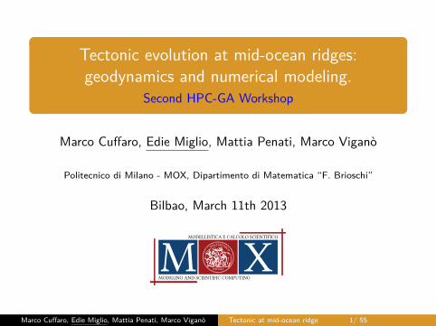
Aims and motivations
Marco Cuffaro, Edie Miglio, Mattia Penati, Marco Viganò Tectonic at mid-ocean ridge 2/ 55
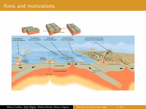
Aims and motivations
Marco Cuffaro, Edie Miglio, Mattia Penati, Marco Viganò Tectonic at mid-ocean ridge 3/ 55
Continental riftAnalogue models
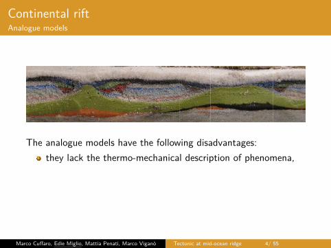
The analogue models have the following disadvantages:they lack the thermo-mechanical description of phenomena,
they are very expensive to setup and perform,they are not general, but specific for a given region,they are not replicable.
Marco Cuffaro, Edie Miglio, Mattia Penati, Marco Viganò Tectonic at mid-ocean ridge 4/ 55
Continental riftAnalogue models
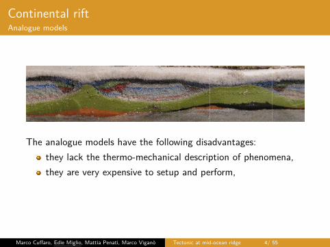
The analogue models have the following disadvantages:they lack the thermo-mechanical description of phenomena,they are very expensive to setup and perform,
they are not general, but specific for a given region,they are not replicable.
Marco Cuffaro, Edie Miglio, Mattia Penati, Marco Viganò Tectonic at mid-ocean ridge 4/ 55

Continental riftAnalogue models
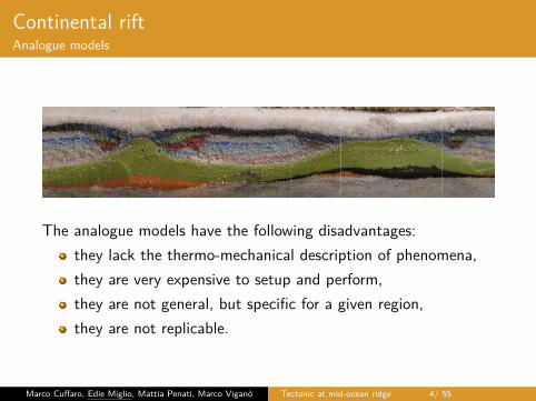
The analogue models have the following disadvantages:they lack the thermo-mechanical description of phenomena,they are very expensive to setup and perform,they are not general, but specific for a given region,
they are not replicable.
Marco Cuffaro, Edie Miglio, Mattia Penati, Marco Viganò Tectonic at mid-ocean ridge 4/ 55
Continental riftAnalogue models
The analogue models have the following disadvantages:they lack the thermo-mechanical description of phenomena,they are very expensive to setup and perform,they are not general, but specific for a given region,they are not replicable.
Marco Cuffaro, Edie Miglio, Mattia Penati, Marco Viganò Tectonic at mid-ocean ridge 4/ 55

Aims and motivations
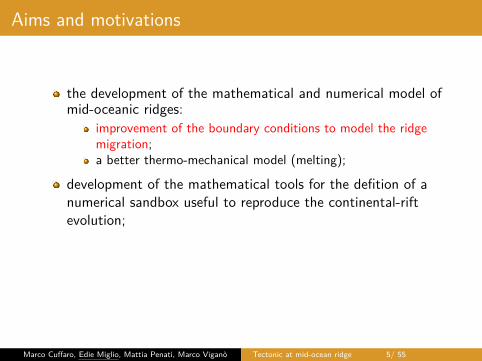
the development of the mathematical and numerical model ofmid-oceanic ridges:
improvement of the boundary conditions to model the ridgemigration;a better thermo-mechanical model (melting);
development of the mathematical tools for the defition of anumerical sandbox useful to reproduce the continental-riftevolution;development and application of meshfree methods andvariational integrators for the simulation of the numericalsandbox.
Marco Cuffaro, Edie Miglio, Mattia Penati, Marco Viganò Tectonic at mid-ocean ridge 5/ 55
Aims and motivations
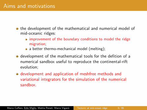
the development of the mathematical and numerical model ofmid-oceanic ridges:
improvement of the boundary conditions to model the ridgemigration;a better thermo-mechanical model (melting);
development of the mathematical tools for the defition of anumerical sandbox useful to reproduce the continental-riftevolution;
development and application of meshfree methods andvariational integrators for the simulation of the numericalsandbox.
Marco Cuffaro, Edie Miglio, Mattia Penati, Marco Viganò Tectonic at mid-ocean ridge 5/ 55
Aims and motivations
the development of the mathematical and numerical model ofmid-oceanic ridges:
improvement of the boundary conditions to model the ridgemigration;a better thermo-mechanical model (melting);
development of the mathematical tools for the defition of anumerical sandbox useful to reproduce the continental-riftevolution;development and application of meshfree methods andvariational integrators for the simulation of the numericalsandbox.
Marco Cuffaro, Edie Miglio, Mattia Penati, Marco Viganò Tectonic at mid-ocean ridge 5/ 55
Mid-ocean ridgesMathematical model
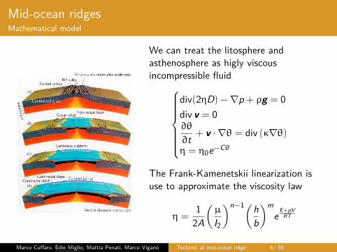
We can treat the litosphere andasthenosphere as higly viscousincompressible fluid
div(2ηD) −∇p + ρg = 0div v = 0∂θ
∂t + v · ∇θ = div (κ∇θ)η = η0e−Cθ
The Frank-Kamenetskii linearization isuse to approximate the viscosity law
η =1
2A
(µ
I2
)n−1(hb
)me
E+pVRT
Marco Cuffaro, Edie Miglio, Mattia Penati, Marco Viganò Tectonic at mid-ocean ridge 6/ 55
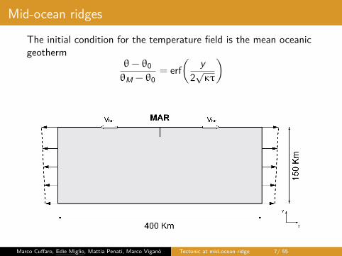
Mid-ocean ridgesThe initial condition for the temperature field is the mean oceanicgeotherm
θ− θ0θM − θ0
= erf(
y2√κτ
)
Marco Cuffaro, Edie Miglio, Mattia Penati, Marco Viganò Tectonic at mid-ocean ridge 7/ 55
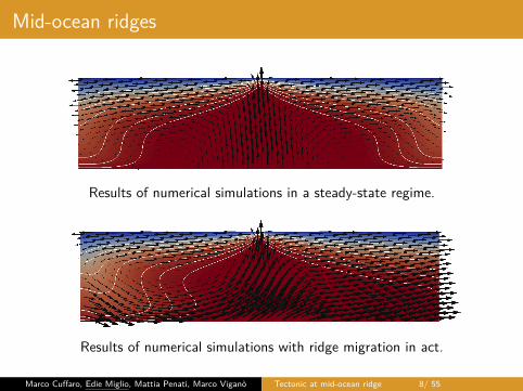
Mid-ocean ridges
Results of numerical simulations in a steady-state regime.
Results of numerical simulations with ridge migration in act.
Marco Cuffaro, Edie Miglio, Mattia Penati, Marco Viganò Tectonic at mid-ocean ridge 8/ 55
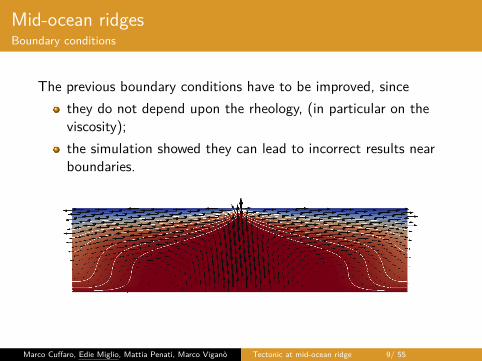
Mid-ocean ridgesBoundary conditions
The previous boundary conditions have to be improved, sincethey do not depend upon the rheology, (in particular on theviscosity);the simulation showed they can lead to incorrect results nearboundaries.
Marco Cuffaro, Edie Miglio, Mattia Penati, Marco Viganò Tectonic at mid-ocean ridge 9/ 55
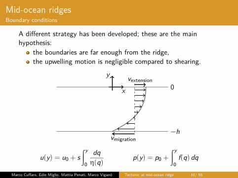
Mid-ocean ridgesBoundary conditions
A different strategy has been developed; these are the mainhypothesis:
the boundaries are far enough from the ridge,the upwelling motion is negligible compared to shearing.
.. 0.
−h
.x
.y
.vextension.
vmigration
u(y) = u0 + s∫ y
0
dqη(q) p(y) = p0 +
∫ y
0f(q) dq
Marco Cuffaro, Edie Miglio, Mattia Penati, Marco Viganò Tectonic at mid-ocean ridge 10/ 55
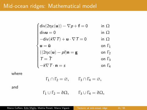
Mid-ocean ridges: Mathematical model
div(2ηε(u)) −∇p + f = 0 in Ωdivu = 0 in Ω−div(k∇T) + u · ∇T = 0 in Ωu = u on Γ1((2ηε(u) − pI)n = g on Γ2T = T on Γ3−k∇T · n = s on Γ4
whereΓ1 ∩ Γ2 = ∅, Γ3 ∩ Γ4 = ∅,
andΓ1 ∪ Γ2 = ∂Ω, Γ3 ∪ Γ4 = ∂Ω,
Marco Cuffaro, Edie Miglio, Mattia Penati, Marco Viganò Tectonic at mid-ocean ridge 11/ 55
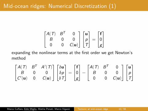
Mid-ocean ridges: Numerical Discretization (1)
A(T) BT 0B 0 00 0 C(u)
upT
=
f0g
expanding the nonlinear terms at the first order we get Newton’smethodA(T) BT A ′(T)
B 0 0C ′(u) 0 C(u)
δuδpδT
=
f0g
−
A(T) BT 0B 0 00 0 C(u)
upT
Marco Cuffaro, Edie Miglio, Mattia Penati, Marco Viganò Tectonic at mid-ocean ridge 12/ 55
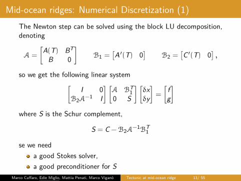
Mid-ocean ridges: Numerical Discretization (1)The Newton step can be solved using the block LU decomposition,denoting
A =
[A(T) BT
B 0
]B1 =
[A ′(T) 0
]B2 =
[C ′(T) 0
],
so we get the following linear system[I 0
B2A−1 I
] [A BT
10 S
] [δxδy
]=
[fg
]where S is the Schur complement,
S = C −B2A−1BT
1
se we needa good Stokes solver,a good preconditioner for S
Marco Cuffaro, Edie Miglio, Mattia Penati, Marco Viganò Tectonic at mid-ocean ridge 13/ 55
Mid-ocean ridges: Preconditioners
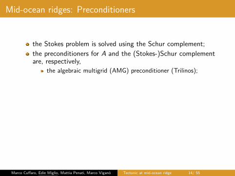
the Stokes problem is solved using the Schur complement;
the preconditioners for A and the (Stokes-)Schur complementare, respectively,
the algebraic multigrid (AMG) preconditioner (Trilinos);the viscosity-scaled pressure mass-matrix.
these preconditioners are almost optimal.The matrix S is preconditioned with the iterative inverse of C(this last problem is preconditioned with AMG preconditioner).this preconditioner seems to scale well with the number ofdegrees of freedom (for each numerical experiments we getabout 10 − 20 iterations to solve the temperature).
Marco Cuffaro, Edie Miglio, Mattia Penati, Marco Viganò Tectonic at mid-ocean ridge 14/ 55
Mid-ocean ridges: Preconditioners
the Stokes problem is solved using the Schur complement;the preconditioners for A and the (Stokes-)Schur complementare, respectively,
the algebraic multigrid (AMG) preconditioner (Trilinos);
the viscosity-scaled pressure mass-matrix.
these preconditioners are almost optimal.The matrix S is preconditioned with the iterative inverse of C(this last problem is preconditioned with AMG preconditioner).this preconditioner seems to scale well with the number ofdegrees of freedom (for each numerical experiments we getabout 10 − 20 iterations to solve the temperature).
Marco Cuffaro, Edie Miglio, Mattia Penati, Marco Viganò Tectonic at mid-ocean ridge 14/ 55
Mid-ocean ridges: Preconditioners
the Stokes problem is solved using the Schur complement;the preconditioners for A and the (Stokes-)Schur complementare, respectively,
the algebraic multigrid (AMG) preconditioner (Trilinos);the viscosity-scaled pressure mass-matrix.
these preconditioners are almost optimal.The matrix S is preconditioned with the iterative inverse of C(this last problem is preconditioned with AMG preconditioner).this preconditioner seems to scale well with the number ofdegrees of freedom (for each numerical experiments we getabout 10 − 20 iterations to solve the temperature).
Marco Cuffaro, Edie Miglio, Mattia Penati, Marco Viganò Tectonic at mid-ocean ridge 14/ 55
Mid-ocean ridges: Preconditioners
the Stokes problem is solved using the Schur complement;the preconditioners for A and the (Stokes-)Schur complementare, respectively,
the algebraic multigrid (AMG) preconditioner (Trilinos);the viscosity-scaled pressure mass-matrix.
these preconditioners are almost optimal.
The matrix S is preconditioned with the iterative inverse of C(this last problem is preconditioned with AMG preconditioner).this preconditioner seems to scale well with the number ofdegrees of freedom (for each numerical experiments we getabout 10 − 20 iterations to solve the temperature).
Marco Cuffaro, Edie Miglio, Mattia Penati, Marco Viganò Tectonic at mid-ocean ridge 14/ 55
Mid-ocean ridges: Preconditioners
the Stokes problem is solved using the Schur complement;the preconditioners for A and the (Stokes-)Schur complementare, respectively,
the algebraic multigrid (AMG) preconditioner (Trilinos);the viscosity-scaled pressure mass-matrix.
these preconditioners are almost optimal.The matrix S is preconditioned with the iterative inverse of C(this last problem is preconditioned with AMG preconditioner).
this preconditioner seems to scale well with the number ofdegrees of freedom (for each numerical experiments we getabout 10 − 20 iterations to solve the temperature).
Marco Cuffaro, Edie Miglio, Mattia Penati, Marco Viganò Tectonic at mid-ocean ridge 14/ 55
Mid-ocean ridges: Preconditioners
the Stokes problem is solved using the Schur complement;the preconditioners for A and the (Stokes-)Schur complementare, respectively,
the algebraic multigrid (AMG) preconditioner (Trilinos);the viscosity-scaled pressure mass-matrix.
these preconditioners are almost optimal.The matrix S is preconditioned with the iterative inverse of C(this last problem is preconditioned with AMG preconditioner).this preconditioner seems to scale well with the number ofdegrees of freedom (for each numerical experiments we getabout 10 − 20 iterations to solve the temperature).
Marco Cuffaro, Edie Miglio, Mattia Penati, Marco Viganò Tectonic at mid-ocean ridge 14/ 55
Mid-ocean ridges: Numerical treatment of stress BC
To compute the stress boundary conditions we use the fixed pointiteration method, with the following scheme
given a solution (u, p,T) the boundary condition g iscomputedfrom g a new solution (u, p,T) is computed
Marco Cuffaro, Edie Miglio, Mattia Penati, Marco Viganò Tectonic at mid-ocean ridge 15/ 55
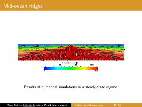
Mid-ocean ridges
Results of numerical simulations in a steady-state regime.
Marco Cuffaro, Edie Miglio, Mattia Penati, Marco Viganò Tectonic at mid-ocean ridge 16/ 55
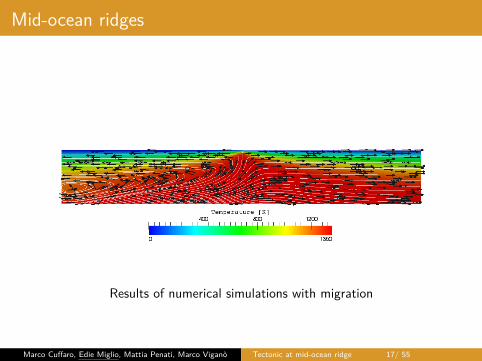
Mid-ocean ridges
Results of numerical simulations with migration
Marco Cuffaro, Edie Miglio, Mattia Penati, Marco Viganò Tectonic at mid-ocean ridge 17/ 55
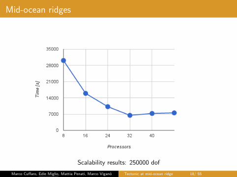
Mid-ocean ridges
Scalability results: 250000 dofMarco Cuffaro, Edie Miglio, Mattia Penati, Marco Viganò Tectonic at mid-ocean ridge 18/ 55
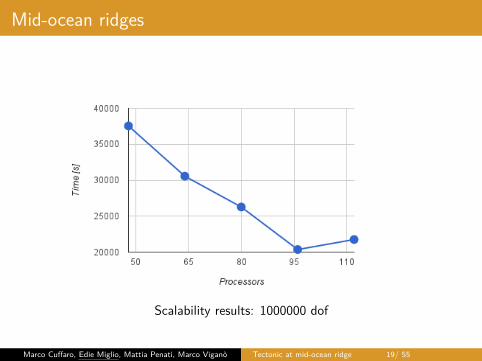
Mid-ocean ridges
Scalability results: 1000000 dof
Marco Cuffaro, Edie Miglio, Mattia Penati, Marco Viganò Tectonic at mid-ocean ridge 19/ 55
Mid-ocean ridges
Marco Cuffaro, Edie Miglio, Mattia Penati, Marco Viganò Tectonic at mid-ocean ridge 20/ 55
Mid-ocean ridges
Marco Cuffaro, Edie Miglio, Mattia Penati, Marco Viganò Tectonic at mid-ocean ridge 21/ 55
Mid-ocean ridges
Marco Cuffaro, Edie Miglio, Mattia Penati, Marco Viganò Tectonic at mid-ocean ridge 22/ 55
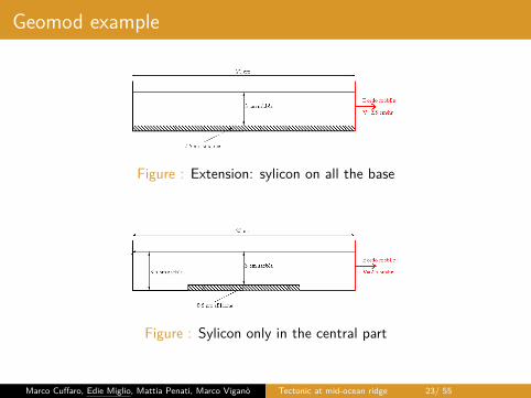
Geomod example
Figure : Extension: sylicon on all the base
Figure : Sylicon only in the central part
Marco Cuffaro, Edie Miglio, Mattia Penati, Marco Viganò Tectonic at mid-ocean ridge 23/ 55
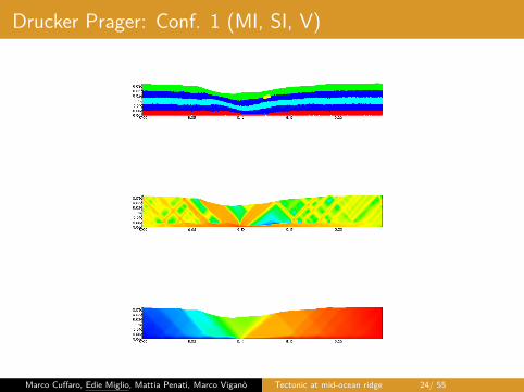
Drucker Prager: Conf. 1 (MI, SI, V)
Marco Cuffaro, Edie Miglio, Mattia Penati, Marco Viganò Tectonic at mid-ocean ridge 24/ 55
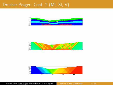
Drucker Prager: Conf. 2 (MI, SI, V)
Marco Cuffaro, Edie Miglio, Mattia Penati, Marco Viganò Tectonic at mid-ocean ridge 25/ 55
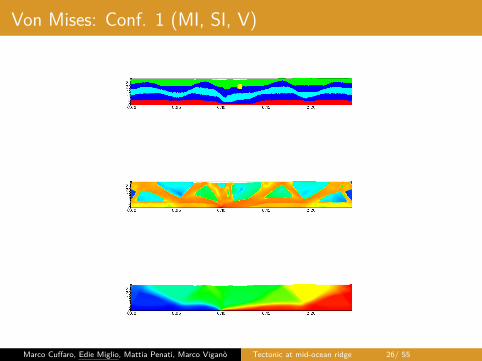
Von Mises: Conf. 1 (MI, SI, V)
Marco Cuffaro, Edie Miglio, Mattia Penati, Marco Viganò Tectonic at mid-ocean ridge 26/ 55
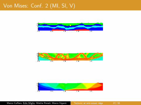
Von Mises: Conf. 2 (MI, SI, V)
Marco Cuffaro, Edie Miglio, Mattia Penati, Marco Viganò Tectonic at mid-ocean ridge 27/ 55
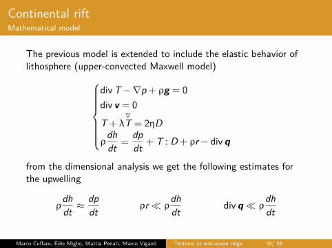
Continental riftMathematical model
The previous model is extended to include the elastic behavior oflithosphere (upper-convected Maxwell model)
div T −∇p + ρg = 0div v = 0
T + λOT = 2ηD
ρdhdt =
dpdt + T : D + ρr − div q
from the dimensional analysis we get the following estimates forthe upwelling
ρdhdt ≈ dp
dt ρr ρdhdt div q ρ
dhdt
Marco Cuffaro, Edie Miglio, Mattia Penati, Marco Viganò Tectonic at mid-ocean ridge 28/ 55
Optimal transportation mesh-free method
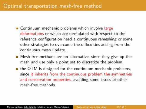
Continuum mechanic problems which involve largedeformations or which are formulated with respect to thereference configuration need a continuous remeshing or someother strategies to overcome the difficulties arising from thecontinuous mesh update.
Mesh-free methods are an alternative, since they give up themesh and use only a point set to discretize the problem.the OTM is designed for the continuum mechanic problems,since it inherits from the continuous problem the symmetriesand conservation properties, avoiding some issues of othermesh-free methods.
Marco Cuffaro, Edie Miglio, Mattia Penati, Marco Viganò Tectonic at mid-ocean ridge 29/ 55
Optimal transportation mesh-free method
Continuum mechanic problems which involve largedeformations or which are formulated with respect to thereference configuration need a continuous remeshing or someother strategies to overcome the difficulties arising from thecontinuous mesh update.Mesh-free methods are an alternative, since they give up themesh and use only a point set to discretize the problem.
the OTM is designed for the continuum mechanic problems,since it inherits from the continuous problem the symmetriesand conservation properties, avoiding some issues of othermesh-free methods.
Marco Cuffaro, Edie Miglio, Mattia Penati, Marco Viganò Tectonic at mid-ocean ridge 29/ 55
Optimal transportation mesh-free method
Continuum mechanic problems which involve largedeformations or which are formulated with respect to thereference configuration need a continuous remeshing or someother strategies to overcome the difficulties arising from thecontinuous mesh update.Mesh-free methods are an alternative, since they give up themesh and use only a point set to discretize the problem.the OTM is designed for the continuum mechanic problems,since it inherits from the continuous problem the symmetriesand conservation properties, avoiding some issues of othermesh-free methods.
Marco Cuffaro, Edie Miglio, Mattia Penati, Marco Viganò Tectonic at mid-ocean ridge 29/ 55
Local maximum-entropy shape functions
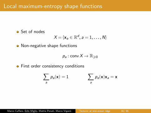
Set of nodesX = xa ∈ Rd, a = 1, . . . ,N
Non-negative shape functions
pa : conv X → R>0
First order consistency conditions∑a
pa(x) = 1∑
apa(x)xa = x
Marco Cuffaro, Edie Miglio, Mattia Penati, Marco Viganò Tectonic at mid-ocean ridge 30/ 55
Local maximum-entropy shape functions
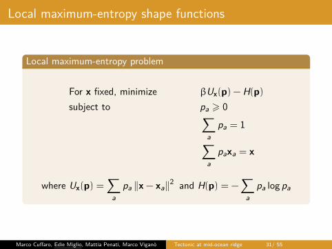
.Local maximum-entropy problem..
.
For x fixed, minimize βUx(p) − H(p)subject to pa > 0∑
apa = 1∑
apaxa = x
where Ux(p) =∑
apa ‖x − xa‖2 and H(p) = −
∑a
pa log pa
Marco Cuffaro, Edie Miglio, Mattia Penati, Marco Viganò Tectonic at mid-ocean ridge 31/ 55
Local maximum-entropy shape functions
.Local maximum-entropy problem..
.
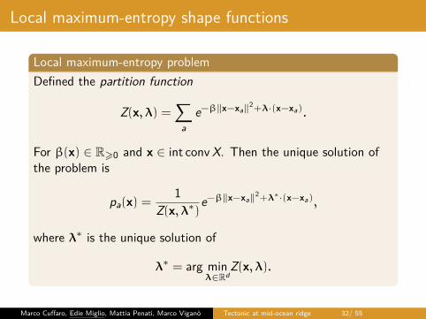
Defined the partition function
Z(x,λ) =∑
ae−β‖x−xa‖2+λ·(x−xa).
For β(x) ∈ R>0 and x ∈ int conv X. Then the unique solution ofthe problem is
pa(x) =1
Z(x,λ∗)e−β‖x−xa‖2+λ∗·(x−xa),
where λ∗ is the unique solution of
λ∗ = arg minλ∈Rd
Z(x,λ).
Marco Cuffaro, Edie Miglio, Mattia Penati, Marco Viganò Tectonic at mid-ocean ridge 32/ 55
Local maximum-entropy shape functions
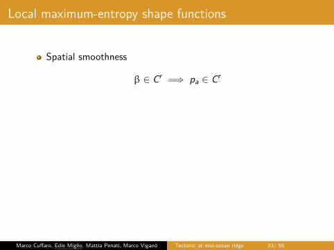
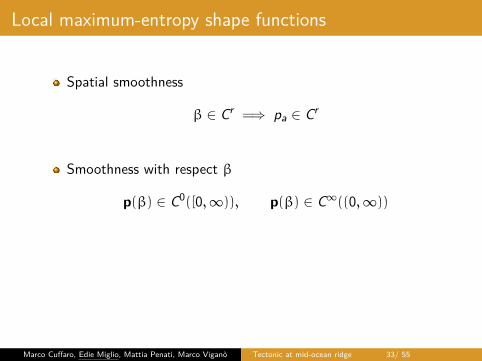
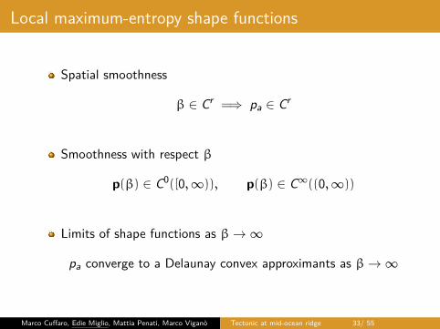
Spatial smoothness
β ∈ Cr =⇒ pa ∈ Cr
Smoothness with respect β
p(β) ∈ C0([0,∞)), p(β) ∈ C∞((0,∞))
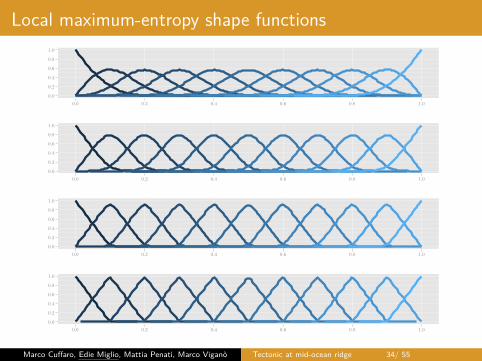
Limits of shape functions as β→ ∞pa converge to a Delaunay convex approximants as β→ ∞
Marco Cuffaro, Edie Miglio, Mattia Penati, Marco Viganò Tectonic at mid-ocean ridge 33/ 55
Local maximum-entropy shape functions
Spatial smoothness
β ∈ Cr =⇒ pa ∈ Cr
Smoothness with respect β
p(β) ∈ C0([0,∞)), p(β) ∈ C∞((0,∞))
Limits of shape functions as β→ ∞pa converge to a Delaunay convex approximants as β→ ∞
Marco Cuffaro, Edie Miglio, Mattia Penati, Marco Viganò Tectonic at mid-ocean ridge 33/ 55
Local maximum-entropy shape functions
0.0
0.2
0.4
0.6
0.8
1.0
0.0 0.2 0.4 0.6 0.8 1.0
0.0
0.2
0.4
0.6
0.8
1.0
0.0 0.2 0.4 0.6 0.8 1.0
0.0
0.2
0.4
0.6
0.8
1.0
0.0 0.2 0.4 0.6 0.8 1.0
0.0
0.2
0.4
0.6
0.8
1.0
0.0 0.2 0.4 0.6 0.8 1.0
Marco Cuffaro, Edie Miglio, Mattia Penati, Marco Viganò Tectonic at mid-ocean ridge 34/ 55
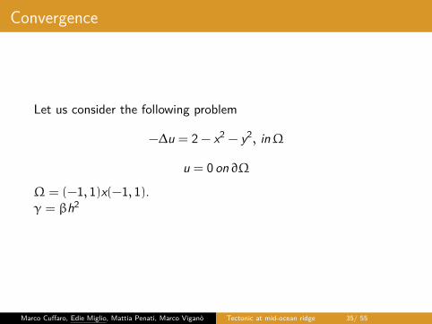
Convergence
Let us consider the following problem
−∆u = 2 − x2 − y2, inΩ
u = 0 on∂Ω
Ω = (−1, 1)x(−1, 1).γ = βh2
Marco Cuffaro, Edie Miglio, Mattia Penati, Marco Viganò Tectonic at mid-ocean ridge 35/ 55
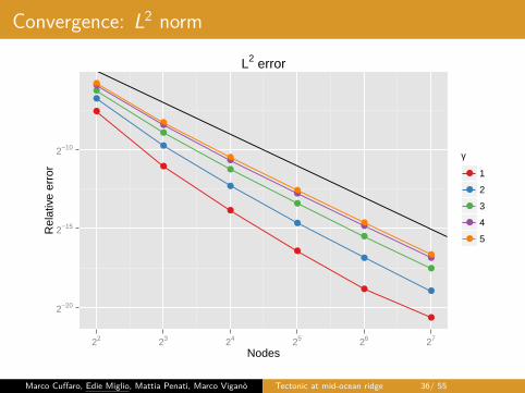
Convergence: L2 norm
2−20
2−15
2−10
22 23 24 25 26 27
Nodes
Rel
ativ
e er
ror
γ
1
2
3
4
5
L2 error
Marco Cuffaro, Edie Miglio, Mattia Penati, Marco Viganò Tectonic at mid-ocean ridge 36/ 55
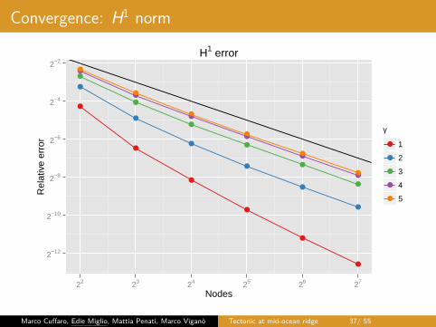
Convergence: H1 norm
2−12
2−10
2−8
2−6
2−4
2−2
22 23 24 25 26 27
Nodes
Rel
ativ
e er
ror
γ
1
2
3
4
5
H1 error
Marco Cuffaro, Edie Miglio, Mattia Penati, Marco Viganò Tectonic at mid-ocean ridge 37/ 55
Optimal transportation
The motion of an inviscid fluid of non-interacting particles in Rd isgoverned by the equations
ρ+ div (ρu) = 0˙(ρu) + div (ρu ⊗ u) = 0
This problem can be recasted as an optimal transportationproblem, that admits a variational formulation
minimize J(ρ,u) =∫b
a
∫Rd
12ρ ‖u‖2 dx dt
subject to ρ+ div (ρu) = 0
Marco Cuffaro, Edie Miglio, Mattia Penati, Marco Viganò Tectonic at mid-ocean ridge 38/ 55
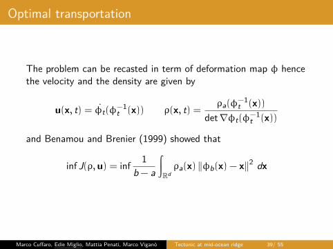
Optimal transportation
The problem can be recasted in term of deformation map φ hencethe velocity and the density are given by
u(x, t) = φt(φ−1t (x)) ρ(x, t) = ρa(φ
−1t (x))
det∇φt(φ−1t (x))
and Benamou and Brenier (1999) showed that
inf J(ρ,u) = inf 1b − a
∫Rdρa(x) ‖φb(x) − x‖2 dx
Marco Cuffaro, Edie Miglio, Mattia Penati, Marco Viganò Tectonic at mid-ocean ridge 39/ 55
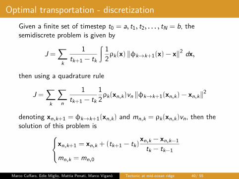
Optimal transportation - discretizationGiven a finite set of timestep t0 = a, t1, t2, . . . , tN = b, thesemidiscrete problem is given by
J =∑
k
1tk+1 − tk
∫ 12ρk(x) ‖φk→k+1(x) − x‖2 dx,
then using a quadrature rule
J =∑
k
∑n
1tk+1 − tk
12ρk(xn,k)vn ‖φk→k+1(xn,k) − xn,k‖2
denoting xn,k+1 = φk→k+1(xn,k) and mn,k = ρk(xn,k)vn, then thesolution of this problem isxn,k+1 = xn,k + (tk+1 − tk)
xn,k − xn,k−1tk − tk−1
mn,k = mn,0
Marco Cuffaro, Edie Miglio, Mattia Penati, Marco Viganò Tectonic at mid-ocean ridge 40/ 55
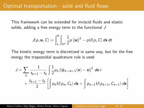
Optimal transportation - solid and fluid flows
This framework can be extended for inviscid fluids and elasticsolids, adding a free energy term to the functional J
J(ρ,u,C) =∫b
a
∫Rd
12ρ ‖u‖2 − ρU(ρ,C) dx dt
The kinetic energy term is discretized in same way, but for the freeenergy the trapezoidal quadrature rule is used
J =∑
k
1tk+1 − tk
∫ 12ρk ‖φk→k+1(x) − x‖2 dx+
+tk+1 − tk
2
[∫ρkU(ρk,Ck) dx +
∫ρk+1U(ρk+1,Ck+1) dx
]
Marco Cuffaro, Edie Miglio, Mattia Penati, Marco Viganò Tectonic at mid-ocean ridge 41/ 55
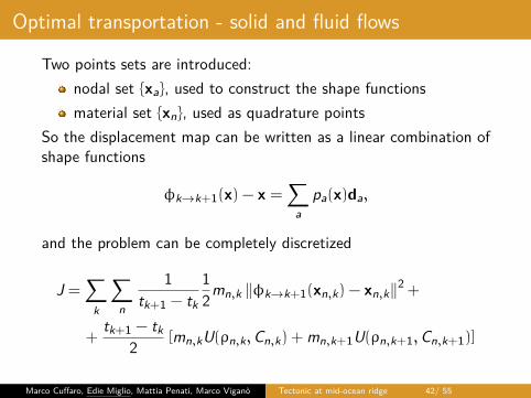
Optimal transportation - solid and fluid flows
Two points sets are introduced:nodal set xa, used to construct the shape functionsmaterial set xn, used as quadrature points
So the displacement map can be written as a linear combination ofshape functions
φk→k+1(x) − x =∑
apa(x)da,
and the problem can be completely discretized
J =∑
k
∑n
1tk+1 − tk
12mn,k ‖φk→k+1(xn,k) − xn,k‖2 +
+tk+1 − tk
2 [mn,kU(ρn,k,Cn,k) + mn,k+1U(ρn,k+1,Cn,k+1)]
Marco Cuffaro, Edie Miglio, Mattia Penati, Marco Viganò Tectonic at mid-ocean ridge 42/ 55
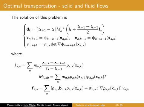
Optimal transportation - solid and fluid flows
The solution of this problem isdk = (tk+1 − tk)M−1
k
(lk +
tk+1 − tk−12 fk
)xn,k+1 = φk→k+1(xn,k), xa,k+1 = φk→k+1(xa,k)
vn,k+1 = vn,k det∇φk→k+1(xa,k)
where
la,k =∑
nmn,k
xn,k − xn,k−1tk − tk−1
pa,k(xn,k)
Mk,ab =∑
nmn,kpa,k(xn,k)pb,k(xn,k)I
fa,k =∑
n[ρn,kbn,kpa,k(xn,k) + σn,k : ∇pa,k(xn,k)] vn,k
Marco Cuffaro, Edie Miglio, Mattia Penati, Marco Viganò Tectonic at mid-ocean ridge 43/ 55
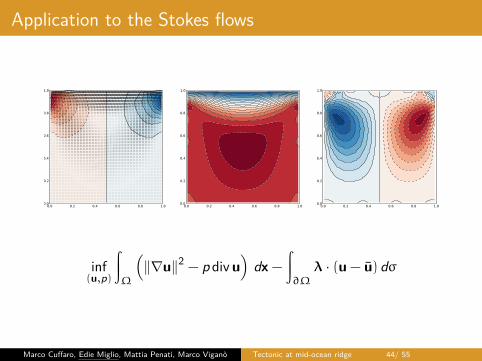
Application to the Stokes flows
0.0 0.2 0.4 0.6 0.8 1.00.0
0.2
0.4
0.6
0.8
1.0
0.0 0.2 0.4 0.6 0.8 1.00.0
0.2
0.4
0.6
0.8
1.0
0.0 0.2 0.4 0.6 0.8 1.00.0
0.2
0.4
0.6
0.8
1.0
inf(u,p)
∫Ω
(‖∇u‖2 − p div u
)dx −
∫∂Ω
λ · (u − u) dσ
Marco Cuffaro, Edie Miglio, Mattia Penati, Marco Viganò Tectonic at mid-ocean ridge 44/ 55
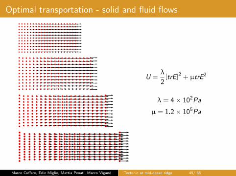
Optimal transportation - solid and fluid flows
U =λ
2 [trE]2 + µtrE2
λ = 4 × 10²Paµ = 1.2 × 10⁵Pa
Marco Cuffaro, Edie Miglio, Mattia Penati, Marco Viganò Tectonic at mid-ocean ridge 45/ 55
Veselov-type discretizationChoosen the discrete set of times
0 = t0 < t1 < t2 < · · · < tN−1 < tN = T
then the motion is described by a sequence of positions
q0, q1, q2, . . . , qN−1, qN
and the discrete action is defined by the sum
Sq =
N−1∑k=0
Ld(qk, qk+1)
where Ld(qk, qk+1) is called discrete Lagrangian, it depends ontwo subsequent positions and it’s a reasonable approximation ofthe action between the configurations qk and qk+1
Ld(qk, qk+1) ≈∫ tk+1
tk
L(q, q) dt
Marco Cuffaro, Edie Miglio, Mattia Penati, Marco Viganò Tectonic at mid-ocean ridge 46/ 55
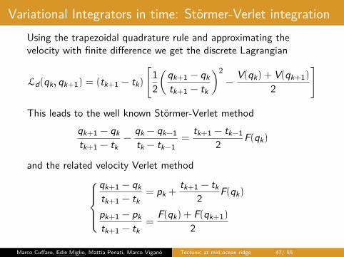
Variational Integrators in time: Störmer-Verlet integrationUsing the trapezoidal quadrature rule and approximating thevelocity with finite difference we get the discrete Lagrangian
Ld(qk, qk+1) = (tk+1 − tk)
[12
(qk+1 − qktk+1 − tk
)2−
V(qk) + V(qk+1)
2
]
This leads to the well known Störmer-Verlet methodqk+1 − qktk+1 − tk
−qk − qk−1tk − tk−1
=tk+1 − tk−1
2 F(qk)
and the related velocity Verlet methodqk+1 − qktk+1 − tk
= pk +tk+1 − tk
2 F(qk)
pk+1 − pktk+1 − tk
=F(qk) + F(qk+1)
2
Marco Cuffaro, Edie Miglio, Mattia Penati, Marco Viganò Tectonic at mid-ocean ridge 47/ 55
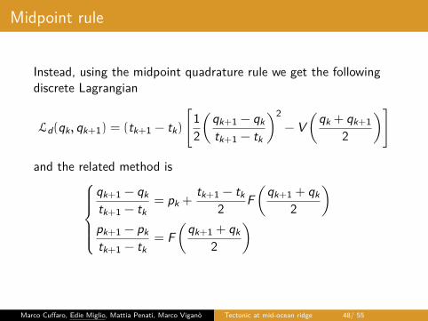
Midpoint rule
Instead, using the midpoint quadrature rule we get the followingdiscrete Lagrangian
Ld(qk, qk+1) = (tk+1 − tk)
[12
(qk+1 − qktk+1 − tk
)2− V
(qk + qk+1
2
)]
and the related method isqk+1 − qktk+1 − tk
= pk +tk+1 − tk
2 F(
qk+1 + qk2
)pk+1 − pktk+1 − tk
= F(
qk+1 + qk2
)
Marco Cuffaro, Edie Miglio, Mattia Penati, Marco Viganò Tectonic at mid-ocean ridge 48/ 55
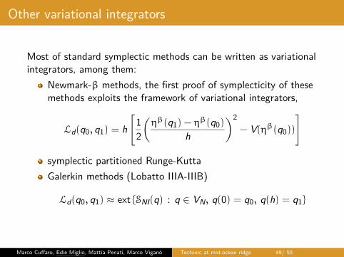
Other variational integrators
Most of standard symplectic methods can be written as variationalintegrators, among them:
Newmark-β methods, the first proof of symplecticity of thesemethods exploits the framework of variational integrators,
Ld(q0, q1) = h[
12
(ηβ(q1) − ηβ(q0)
h
)2− V(ηβ(q0))
]
symplectic partitioned Runge-KuttaGalerkin methods (Lobatto IIIA-IIIB)
Ld(q0, q1) ≈ ext SNI(q) : q ∈ VN, q(0) = q0, q(h) = q1
Marco Cuffaro, Edie Miglio, Mattia Penati, Marco Viganò Tectonic at mid-ocean ridge 49/ 55
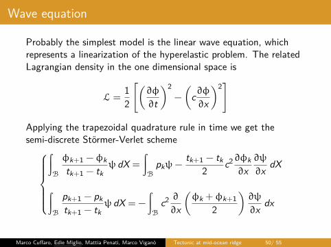
Wave equation
Probably the simplest model is the linear wave equation, whichrepresents a linearization of the hyperelastic problem. The relatedLagrangian density in the one dimensional space is
L =12
[(∂φ
∂t
)2−
(c∂φ∂x
)2]
Applying the trapezoidal quadrature rule in time we get thesemi-discrete Störmer-Verlet scheme
∫B
φk+1 − φktk+1 − tk
ψ dX =
∫B
pkψ−tk+1 − tk
2 c2∂φk∂x
∂ψ
∂x dX
∫B
pk+1 − pktk+1 − tk
ψ dX = −
∫B
c2 ∂
∂x
(φk + φk+1
2
)∂ψ
∂x dx
Marco Cuffaro, Edie Miglio, Mattia Penati, Marco Viganò Tectonic at mid-ocean ridge 50/ 55
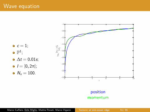
Wave equation
c = 1;P1;∆t = 0.01s;I = [0, 2π];Nx = 100.
0 2 4 6 8 10t
−24
−22
−20
−18
−16
−14
−12
−10
−8
log
2
‖uh−u‖ 2
‖u‖ 2
positionmomentum
Marco Cuffaro, Edie Miglio, Mattia Penati, Marco Viganò Tectonic at mid-ocean ridge 51/ 55
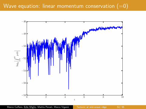
Wave equation: linear momentum conservation (=0)
0 2 4 6 8 10t
−58
−56
−54
−52
−50
−48
−46
log
2
∣ ∣ ∣ ∣∫2π
0
pdx
∣ ∣ ∣ ∣
Marco Cuffaro, Edie Miglio, Mattia Penati, Marco Viganò Tectonic at mid-ocean ridge 52/ 55
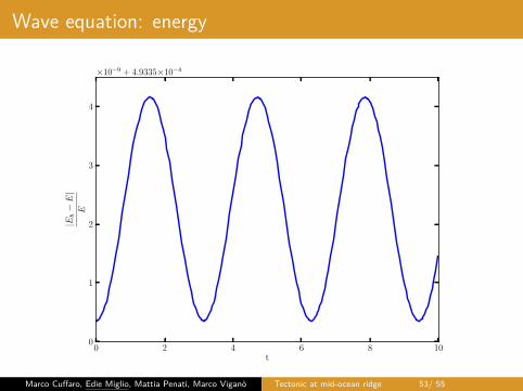
Wave equation: energy
0 2 4 6 8 10t
0
1
2
3
4
|Eh−E|
E×10−9 + 4.9335×10⁻⁴
Marco Cuffaro, Edie Miglio, Mattia Penati, Marco Viganò Tectonic at mid-ocean ridge 53/ 55
Conclusions and further developments
improvement of BC treatment;preconditioners;preliminary results on OTM.
Future developments of this projectintroduction of the melting;development of a fluid-structure and structure-structuremethod based on OTM;application of OTM and VI to geodynamic problems, couplingthe mechanical problem with the thermodynamic.
Marco Cuffaro, Edie Miglio, Mattia Penati, Marco Viganò Tectonic at mid-ocean ridge 54/ 55
Thank you for your attention!
Marco Cuffaro, Edie Miglio, Mattia Penati, Marco Viganò Tectonic at mid-ocean ridge 55/ 55