Embed Size (px)
Citation preview

Second Edition
Reservoir Eng FOB 2001-10-29 16:18 Page i
Naturally occurring hydrocarbon systems found in petroleum reser-voirs are mixtures of organic compounds which exhibit multiphasebehavior over wide ranges of pressures and temperatures. These hydro-carbon accumulations may occur in the gaseous state, the liquid state, thesolid state, or in various combinations of gas, liquid, and solid.
These differences in phase behavior, coupled with the physical proper-ties of reservoir rock that determine the relative ease with which gas andliquid are transmitted or retained, result in many diverse types of hydro-carbon reservoirs with complex behaviors. Frequently, petroleum engi-neers have the task to study the behavior and characteristics of a petrole-um reservoir and to determine the course of future development andproduction that would maximize the profit.
The objective of this chapter is to review the basic principles of reser-voir fluid phase behavior and illustrate the use of phase diagrams in clas-sifying types of reservoirs and the native hydrocarbon systems.
CLASSIFICATION OF RESERVOIRSAND RESERVOIR FLUIDS
Petroleum reservoirs are broadly classified as oil or gas reservoirs.These broad classifications are further subdivided depending on:
1
C H A P T E R 1
FUNDAMENTALS OFRESERVOIR FLUID
BEHAVIOR
Reservoir Eng Hndbk Ch 01 2001-10-24 09:04 Page 1

• The composition of the reservoir hydrocarbon mixture• Initial reservoir pressure and temperature• Pressure and temperature of the surface production
The conditions under which these phases exist are a matter of consid-erable practical importance. The experimental or the mathematical deter-minations of these conditions are conveniently expressed in differenttypes of diagrams commonly called phase diagrams. One such diagramis called the pressure-temperature diagram.
Pressure-Temperature Diagram
Figure 1-1 shows a typical pressure-temperature diagram of a multi-component system with a specific overall composition. Although a dif-ferent hydrocarbon system would have a different phase diagram, thegeneral configuration is similar.
2 Reservoir Engineering Handbook
Liquid
Gas
C
100%Liquid
90%
70%
50%
5% 0%F B
A
E
Bubbl
e-po
int C
urve
Dew
-poi
nt C
urve
Two-phase Region
Temperature
Critical Poi
Pre
ssur
e
Figure 1-1. Typical p-T diagram for a multicomponent system.
Reservoir Eng Hndbk Ch 01 2001-10-24 09:04 Page 2

These multicomponent pressure-temperature diagrams are essentiallyused to:
• Classify reservoirs• Classify the naturally occurring hydrocarbon systems• Describe the phase behavior of the reservoir fluid
To fully understand the significance of the pressure-temperature dia-grams, it is necessary to identify and define the following key points onthese diagrams:
• Cricondentherm (Tct)—The Cricondentherm is defined as the maxi-mum temperature above which liquid cannot be formed regardless ofpressure (point E). The corresponding pressure is termed the Cricon-dentherm pressure pct.
• Cricondenbar (pcb)—The Cricondenbar is the maximum pressure abovewhich no gas can be formed regardless of temperature (point D). Thecorresponding temperature is called the Cricondenbar temperature Tcb.
• Critical point—The critical point for a multicomponent mixture isreferred to as the state of pressure and temperature at which all inten-sive properties of the gas and liquid phases are equal (point C). At thecritical point, the corresponding pressure and temperature are called thecritical pressure pc and critical temperature Tc of the mixture.
• Phase envelope (two-phase region)—The region enclosed by the bub-ble-point curve and the dew-point curve (line BCA), wherein gas andliquid coexist in equilibrium, is identified as the phase envelope of thehydrocarbon system.
• Quality lines—The dashed lines within the phase diagram are calledquality lines. They describe the pressure and temperature conditions forequal volumes of liquids. Note that the quality lines converge at thecritical point (point C).
• Bubble-point curve—The bubble-point curve (line BC) is defined asthe line separating the liquid-phase region from the two-phase region.
• Dew-point curve—The dew-point curve (line AC) is defined as theline separating the vapor-phase region from the two-phase region.
In general, reservoirs are conveniently classified on the basis of thelocation of the point representing the initial reservoir pressure pi and tem-perature T with respect to the pressure-temperature diagram of the reser-voir fluid. Accordingly, reservoirs can be classified into basically twotypes. These are:
Fundamentals of Reservoir Fluid Behavior 3
Reservoir Eng Hndbk Ch 01 2001-10-24 09:04 Page 3
• Oil reservoirs—If the reservoir temperature T is less than the criticaltemperature Tc of the reservoir fluid, the reservoir is classified as an oilreservoir.
• Gas reservoirs—If the reservoir temperature is greater than the criticaltemperature of the hydrocarbon fluid, the reservoir is considered a gasreservoir.
Oil Reservoirs
Depending upon initial reservoir pressure pi, oil reservoirs can be sub-classified into the following categories:
1. Undersaturated oil reservoir. If the initial reservoir pressure pi (asrepresented by point 1 on Figure 1-1), is greater than the bubble-pointpressure pb of the reservoir fluid, the reservoir is labeled an undersatu-rated oil reservoir.
2. Saturated oil reservoir. When the initial reservoir pressure is equal tothe bubble-point pressure of the reservoir fluid, as shown on Figure 1-1by point 2, the reservoir is called a saturated oil reservoir.
3. Gas-cap reservoir. If the initial reservoir pressure is below the bubble-point pressure of the reservoir fluid, as indicated by point 3 on Figure 1-1, the reservoir is termed a gas-cap or two-phase reservoir, in whichthe gas or vapor phase is underlain by an oil phase. The appropriatequality line gives the ratio of the gas-cap volume to reservoir oil volume.
Crude oils cover a wide range in physical properties and chemicalcompositions, and it is often important to be able to group them intobroad categories of related oils. In general, crude oils are commonly clas-sified into the following types:
• Ordinary black oil• Low-shrinkage crude oil• High-shrinkage (volatile) crude oil• Near-critical crude oil
The above classifications are essentially based upon the propertiesexhibited by the crude oil, including physical properties, composition,gas-oil ratio, appearance, and pressure-temperature phase diagrams.
1. Ordinary black oil. A typical pressure-temperature phase diagram forordinary black oil is shown in Figure 1-2. It should be noted that quali-ty lines which are approximately equally spaced characterize this
4 Reservoir Engineering Handbook
Reservoir Eng Hndbk Ch 01 2001-10-24 09:04 Page 4

black oil phase diagram. Following the pressure reduction path as indi-cated by the vertical line EF on Figure 1-2, the liquid shrinkage curve,as shown in Figure 1-3, is prepared by plotting the liquid volume per-cent as a function of pressure. The liquid shrinkage curve approxi-mates a straight line except at very low pressures. When produced,ordinary black oils usually yield gas-oil ratios between 200–700scf/STB and oil gravities of 15 to 40 API. The stock tank oil is usuallybrown to dark green in color.
2. Low-shrinkage oil. A typical pressure-temperature phase diagram forlow-shrinkage oil is shown in Figure 1-4. The diagram is characterizedby quality lines that are closely spaced near the dew-point curve. Theliquid-shrinkage curve, as given in Figure 1-5, shows the shrinkagecharacteristics of this category of crude oils. The other associatedproperties of this type of crude oil are:
• Oil formation volume factor less than 1.2 bbl/STB• Gas-oil ratio less than 200 scf/STB• Oil gravity less than 35° API• Black or deeply colored
Fundamentals of Reservoir Fluid Behavior 5
Liquid
Gas
C
100%Liquid
90%
70%
50%
5% 0%F B
A
EBub
ble-
poin
t Cur
ve
Dew
-poi
nt C
urve
Two-phase Region
Temperature
Critical Point
Pre
ssur
e
Figure 1-2. A typical p-T diagram for an ordinary black oil.
Reservoir Eng Hndbk Ch 01 2001-10-24 09:04 Page 5

6 Reservoir Engineering Handbook
Residual Oil
E
F
100%
0%Pressure
Liq
uid
Vo
lum
e
Figure 1-3. Liquid-shrinkage curve for black oil.
Liquid
Gas
C100%
85%
A
G
75%
65%0%
FB
E
Bubble-point Curve
Dew
-poi
nt C
urve
Separator Conditions
Temperature
Critical Point
Pre
ssur
e
Figure 1-4. A typical phase diagram for a low-shrinkage oil.
• Substantial liquid recovery at separator conditions as indicated bypoint G on the 85% quality line of Figure 1-4.
3. Volatile crude oil. The phase diagram for a volatile (high-shrinkage)crude oil is given in Figure 1-6. Note that the quality lines are close
Reservoir Eng Hndbk Ch 01 2001-10-24 09:04 Page 6

together near the bubble-point and are more widely spaced at lowerpressures. This type of crude oil is commonly characterized by a highliquid shrinkage immediately below the bubble-point as shown in Fig-ure 1-7. The other characteristic properties of this oil include:
Fundamentals of Reservoir Fluid Behavior 7
Residual Oil
E
F
100%
0%Pressure
Liq
uid
Vo
lum
e
Figure 1-5. Oil-shrinkage curve for low-shrinkage oil.
Critical Point
Dew
-poi
nt C
urve
Bubb
le-p
oint
Cur
ve
Temperature
A
BFG
E
70%60%
50%
0%
C
Gas
Liquid
50%
100%LiquidP
ress
ure
Two-phase Region
SeparatorCondition
Figure 1-6. A typical p-T diagram for a volatile crude oil.
Reservoir Eng Hndbk Ch 01 2001-10-24 09:04 Page 7
8 Reservoir Engineering Handbook
Residual Oil
E
F
100%
0%Pressure
Liq
uid
Vo
lum
e %
Figure 1-7. A typical liquid-shrinkage curve for a volatile crude oil.
• Oil formation volume factor less than 2 bbl/STB• Gas-oil ratios between 2,000–3,200 scf/STB• Oil gravities between 45–55° API• Lower liquid recovery of separator conditions as indicated by point
G on Figure 1-6• Greenish to orange in color
Another characteristic of volatile oil reservoirs is that the API gravityof the stock-tank liquid will increase in the later life of the reservoirs.
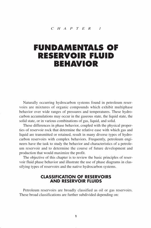
4. Near-critical crude oil. If the reservoir temperature T is near the criti-cal temperature Tc of the hydrocarbon system, as shown in Figure 1-8,the hydrocarbon mixture is identified as a near-critical crude oil.Because all the quality lines converge at the critical point, an isothermalpressure drop (as shown by the vertical line EF in Figure 1-8) mayshrink the crude oil from 100% of the hydrocarbon pore volume at thebubble-point to 55% or less at a pressure 10 to 50 psi below the bubble-point. The shrinkage characteristic behavior of the near-critical crude oilis shown in Figure 1-9. The near-critical crude oil is characterized by ahigh GOR in excess of 3,000 scf/STB with an oil formation volume fac-tor of 2.0 bbl/STB or higher. The compositions of near-critical oils areusually characterized by 12.5 to 20 mol% heptanes-plus, 35% or moreof ethane through hexanes, and the remainder methane.
Reservoir Eng Hndbk Ch 01 2001-10-24 09:04 Page 8

Fundamentals of Reservoir Fluid Behavior 9
Liquid
Gas
C
100%Liquid
50%
0% LiquidF B
A
E
Bubbl
e-po
int C
urve
Dew
-po
int
Cur
veTemperature
Critical Point
Pre
ssur
e
Two-phase Region
Figure 1-8. A schematic phase diagram for the near-critical crude oil.
E
F
100%
0%Pressure
Liq
uid
Vo
lum
e %
Figure 1-9. A typical liquid-shrinkage curve for the near-critical crude oil.
Reservoir Eng Hndbk Ch 01 2001-10-24 09:04 Page 9

Figure 1-10 compares the characteristic shape of the liquid-shrinkagecurve for each crude oil type.
Gas Reservoirs
In general, if the reservoir temperature is above the critical tempera-ture of the hydrocarbon system, the reservoir is classified as a natural gasreservoir. On the basis of their phase diagrams and the prevailing reser-voir conditions, natural gases can be classified into four categories:
• Retrograde gas-condensate• Near-critical gas-condensate• Wet gas• Dry gas
Retrograde gas-condensate reservoir. If the reservoir temperature Tlies between the critical temperature Tc and cricondentherm Tct of thereservoir fluid, the reservoir is classified as a retrograde gas-condensatereservoir. This category of gas reservoir is a unique type of hydrocarbonaccumulation in that the special thermodynamic behavior of the reservoirfluid is the controlling factor in the development and the depletionprocess of the reservoir. When the pressure is decreased on these mix-
10 Reservoir Engineering Handbook
Figure 1-10. Liquid shrinkage for crude oil systems.
Reservoir Eng Hndbk Ch 01 2001-10-24 09:04 Page 10

tures, instead of expanding (if a gas) or vaporizing (if a liquid) as mightbe expected, they vaporize instead of condensing.
Consider that the initial condition of a retrograde gas reservoir is rep-resented by point 1 on the pressure-temperature phase diagram of Figure1-11. Because the reservoir pressure is above the upper dew-point pres-sure, the hydrocarbon system exists as a single phase (i.e., vapor phase)in the reservoir. As the reservoir pressure declines isothermally duringproduction from the initial pressure (point 1) to the upper dew-pointpressure (point 2), the attraction between the molecules of the light andheavy components causes them to move further apart further apart. Asthis occurs, attraction between the heavy component molecules becomesmore effective; thus, liquid begins to condense.
This retrograde condensation process continues with decreasing pres-sure until the liquid dropout reaches its maximum at point 3. Furtherreduction in pressure permits the heavy molecules to commence the nor-mal vaporization process. This is the process whereby fewer gas mole-cules strike the liquid surface and causes more molecules to leave than
Fundamentals of Reservoir Fluid Behavior 11
Liquid
Bubble-point C
urve
Two-phase Region
Temperature
Pre
ssur
e
Upper Dew-point Curve
C 12
Lower Dew-point Curve
Tc Tct
4
3
Figure 1-11. A typical phase diagram of a retrograde system.
Reservoir Eng Hndbk Ch 01 2001-10-24 09:04 Page 11
enter the liquid phase. The vaporization process continues until the reser-voir pressure reaches the lower dew-point pressure. This means that allthe liquid that formed must vaporize because the system is essentially allvapors at the lower dew point.
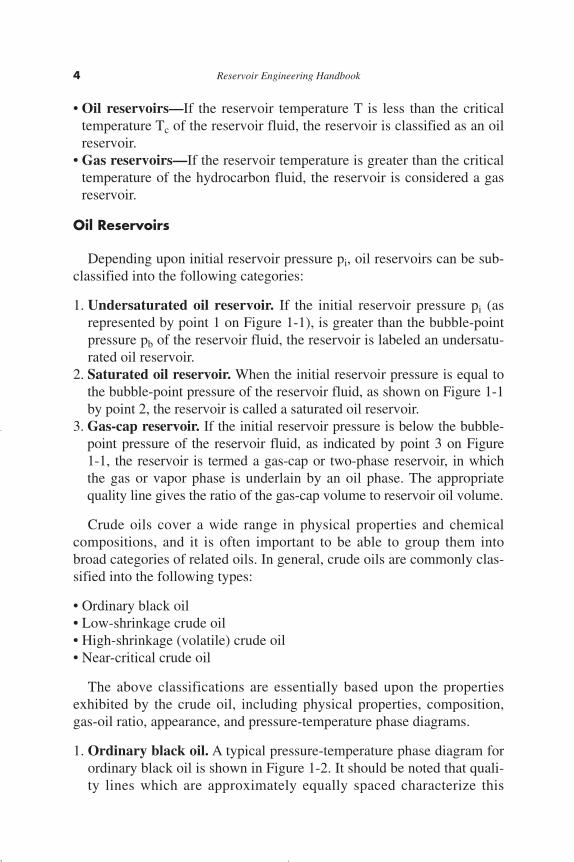
Figure 1-12 shows a typical liquid shrinkage volume curve for a con-densate system. The curve is commonly called the liquid dropout curve.In most gas-condensate reservoirs, the condensed liquid volume seldomexceeds more than 15%–19% of the pore volume. This liquid saturationis not large enough to allow any liquid flow. It should be recognized,however, that around the wellbore where the pressure drop is high,enough liquid dropout might accumulate to give two-phase flow of gasand retrograde liquid.
The associated physical characteristics of this category are:
• Gas-oil ratios between 8,000 to 70,000 scf/STB. Generally, the gas-oilratio for a condensate system increases with time due to the liquiddropout and the loss of heavy components in the liquid.
• Condensate gravity above 50° API• Stock-tank liquid is usually water-white or slightly colored.
There is a fairly sharp dividing line between oils and condensates froma compositional standpoint. Reservoir fluids that contain heptanes andare heavier in concentrations of more than 12.5 mol% are almost alwaysin the liquid phase in the reservoir. Oils have been observed with hep-
12 Reservoir Engineering Handbook
100
0Pressure
Liq
uid
Vo
lum
e %
Maximum Liquid Dropout
Figure 1-12. A typical liquid dropout curve.
Reservoir Eng Hndbk Ch 01 2001-10-24 09:04 Page 12

tanes and heavier concentrations as low as 10% and condensates as highas 15.5%. These cases are rare, however, and usually have very high tankliquid gravities.
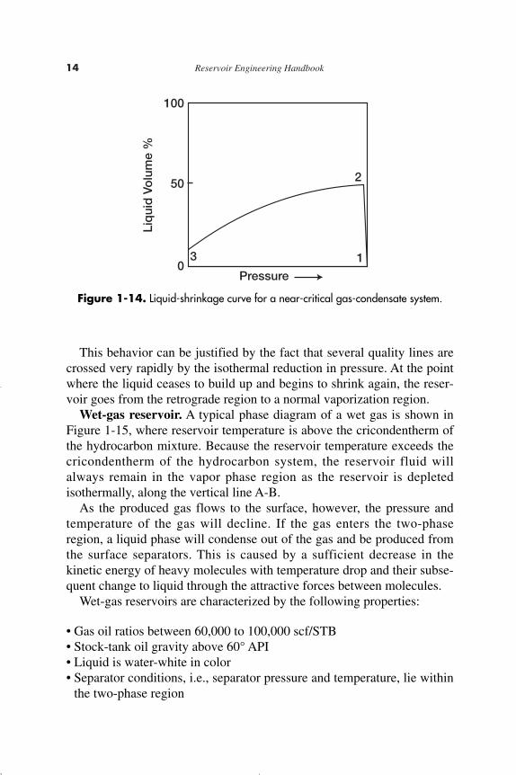
Near-critical gas-condensate reservoir. If the reservoir temperatureis near the critical temperature, as shown in Figure 1-13, the hydrocarbonmixture is classified as a near-critical gas-condensate. The volumetricbehavior of this category of natural gas is described through the isother-mal pressure declines as shown by the vertical line 1-3 in Figure 1-13and also by the corresponding liquid dropout curve of Figure 1-14.Because all the quality lines converge at the critical point, a rapid liquidbuildup will immediately occur below the dew point (Figure 1-14) as thepressure is reduced to point 2.
Fundamentals of Reservoir Fluid Behavior 13
Liquid
Gas
C
100%
0%
1
2
3
Temperature
Critical Point
Pre
ssur
e Two-phase Region
Figure 1-13. A typical phase diagram for a near-critical gas condensate reservoir.
Reservoir Eng Hndbk Ch 01 2001-10-24 09:04 Page 13
14 Reservoir Engineering Handbook
100
03
2
1
50
Pressure
Liq
uid
Vo
lum
e %
Figure 1-14. Liquid-shrinkage curve for a near-critical gas-condensate system.
This behavior can be justified by the fact that several quality lines arecrossed very rapidly by the isothermal reduction in pressure. At the pointwhere the liquid ceases to build up and begins to shrink again, the reser-voir goes from the retrograde region to a normal vaporization region.
Wet-gas reservoir. A typical phase diagram of a wet gas is shown inFigure 1-15, where reservoir temperature is above the cricondentherm ofthe hydrocarbon mixture. Because the reservoir temperature exceeds thecricondentherm of the hydrocarbon system, the reservoir fluid willalways remain in the vapor phase region as the reservoir is depletedisothermally, along the vertical line A-B.
As the produced gas flows to the surface, however, the pressure andtemperature of the gas will decline. If the gas enters the two-phaseregion, a liquid phase will condense out of the gas and be produced fromthe surface separators. This is caused by a sufficient decrease in thekinetic energy of heavy molecules with temperature drop and their subse-quent change to liquid through the attractive forces between molecules.
Wet-gas reservoirs are characterized by the following properties:
• Gas oil ratios between 60,000 to 100,000 scf/STB• Stock-tank oil gravity above 60° API• Liquid is water-white in color• Separator conditions, i.e., separator pressure and temperature, lie within
the two-phase region
Reservoir Eng Hndbk Ch 01 2001-10-24 09:04 Page 14

Dry-gas reservoir. The hydrocarbon mixture exists as a gas both inthe reservoir and in the surface facilities. The only liquid associated withthe gas from a dry-gas reservoir is water. A phase diagram of a dry-gasreservoir is given in Figure 1-16. Usually a system having a gas-oil ratiogreater than 100,000 scf/STB is considered to be a dry gas.
Kinetic energy of the mixture is so high and attraction between mole-cules so small that none of them coalesce to a liquid at stock-tank condi-tions of temperature and pressure.
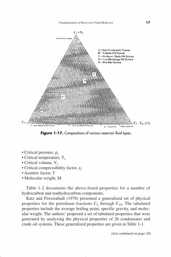
It should be pointed out that the classification of hydrocarbon fluidsmight be also characterized by the initial composition of the system.McCain (1994) suggested that the heavy components in the hydrocarbonmixtures have the strongest effect on fluid characteristics. The ternarydiagram, as shown in Figure 1-17, with equilateral triangles can be con-veniently used to roughly define the compositional boundaries that sepa-rate different types of hydrocarbon systems.
Fundamentals of Reservoir Fluid Behavior 15
Liquid
Gas
Separator
Pressure Depletion atReservoir Temperature
C
75
50
25
5
0
Two-phase Region
Temperature
Pre
ssur
e
B
A
Figure 1-15. Phase diagram for a wet gas. (After Clark, N.J. Elements of PetroleumReservoirs, SPE, 1969.)
Reservoir Eng Hndbk Ch 01 2001-10-24 09:04 Page 15

From the foregoing discussion, it can be observed that hydrocarbonmixtures may exist in either the gaseous or liquid state, depending on thereservoir and operating conditions to which they are subjected. The qual-itative concepts presented may be of aid in developing quantitativeanalyses. Empirical equations of state are commonly used as a quantita-tive tool in describing and classifying the hydrocarbon system. Theseequations of state require:
• Detailed compositional analyses of the hydrocarbon system• Complete descriptions of the physical and critical properties of the mix-
ture individual components
Many characteristic properties of these individual components (inother words, pure substances) have been measured and compiled over theyears. These properties provide vital information for calculating the ther-modynamic properties of pure components, as well as their mixtures. Themost important of these properties are:
16 Reservoir Engineering Handbook
Liquid
Gas
Separator
Pressure Depletion atReservoir Temperature
C
75 50
25 0
Temperature
Pre
ssur
e
B
A
Figure 1-16. Phase diagram for a dry gas. (After Clark, N.J. Elements of PetroleumReservoirs, SPE, 1969.)
Reservoir Eng Hndbk Ch 01 2001-10-24 09:04 Page 16
• Critical pressure, pc
• Critical temperature, Tc
• Critical volume, Vc
• Critical compressibility factor, zc
• Acentric factor, T• Molecular weight, M
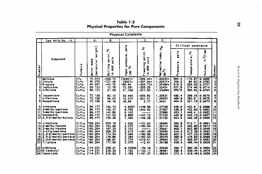
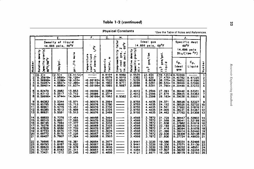
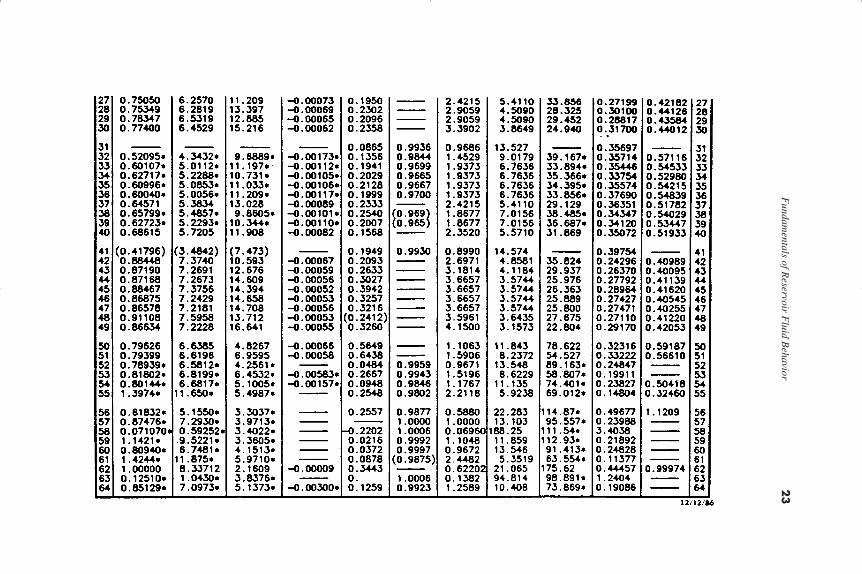
Table 1-2 documents the above-listed properties for a number ofhydrocarbon and nonhydrocarbon components.
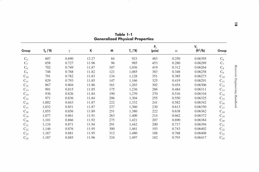
Katz and Firoozabadi (1978) presented a generalized set of physicalproperties for the petroleum fractions C6 through C45. The tabulatedproperties include the average boiling point, specific gravity, and molec-ular weight. The authors’ proposed a set of tabulated properties that weregenerated by analyzing the physical properties of 26 condensates andcrude oil systems. These generalized properties are given in Table 1-1.
Fundamentals of Reservoir Fluid Behavior 17
Figure 1-17. Compositions of various reservoir fluid types.
(text continued on page 24)
Reservoir Eng Hndbk Ch 01 2001-10-24 09:04 Page 17
18
Reservoir E
ngineering Handbook
Table 1-1Generalized Physical Properties
Pc VcGroup Tb (°R) g K M Tc (°R) (psia) w (ft3/lb) Group
C6 607 0.690 12.27 84 923 483 0.250 0.06395 C6
C7 658 0.727 11.96 96 985 453 0.280 0.06289 C7
C8 702 0.749 11.87 107 1,036 419 0.312 0.06264 C8
C9 748 0.768 11.82 121 1,085 383 0.348 0.06258 C9
C10 791 0.782 11.83 134 1,128 351 0.385 0.06273 C10
C11 829 0.793 11.85 147 1,166 325 0.419 0.06291 C11
C12 867 0.804 11.86 161 1,203 302 0.454 0.06306 C12
C13 901 0.815 11.85 175 1,236 286 0.484 0.06311 C13
C14 936 0.826 11.84 190 1,270 270 0.516 0.06316 C14
C15 971 0.836 11.84 206 1,304 255 0.550 0.06325 C15
C16 1,002 0.843 11.87 222 1,332 241 0.582 0.06342 C16
C17 1,032 0.851 11.87 237 1,360 230 0.613 0.06350 C17
C18 1,055 0.856 11.89 251 1,380 222 0.638 0.06362 C18
C19 1,077 0.861 11.91 263 1,400 214 0.662 0.06372 C19
C20 1,101 0.866 11.92 275 1,421 207 0.690 0.06384 C20
C21 1,124 0.871 11.94 291 1,442 200 0.717 0.06394 C21
C22 1,146 0.876 11.95 300 1,461 193 0.743 0.06402 C22
C23 1,167 0.881 11.95 312 1,480 188 0.768 0.06408 C23
C24 1,187 0.885 11.96 324 1,497 182 0.793 0.06417 C24
Reservoir Eng Hndbk Ch 01 2
001-10-24 0
9:04 P
age 18

Fundam
entals of Reservoir F
luid Behavior
19
C25 1,207 0.888 11.99 337 1,515 177 0.819 0.06431 C25
C26 1,226 0.892 12.00 349 1,531 173 0.844 0.06438 C26
C27 1,244 0.896 12.00 360 1,547 169 0.868 0.06443 C27
C28 1,262 0.899 12.02 372 1,562 165 0.894 0.06454 C28
C29 1,277 0.902 12.03 382 1,574 161 0.915 0.06459 C29
C30 1,294 0.905 12.04 394 1,589 158 0.941 0.06468 C30
C31 1,310 0.909 12.04 404 1,603 143 0.897 0.06469 C31
C32 1,326 0.912 12.05 415 1,616 138 0.909 0.06475 C32
C33 1,341 0.915 12.05 426 1,629 134 0.921 0.06480 C33
C34 1,355 0.917 12.07 437 1,640 130 0.932 0.06489 C34
C35 1,368 0.920 12.07 445 1,651 127 0.942 0.06490 C35
C36 1,382 0.922 12.08 456 1,662 124 0.954 0.06499 C36
C37 1,394 0.925 12.08 464 1,673 121 0.964 0.06499 C37
C38 1,407 0.927 12.09 475 1,683 118 0.975 0.06506 C38
C39 1,419 0.929 12.10 484 1,693 115 0.985 0.06511 C39
C40 1,432 0.931 12.11 495 1,703 112 0.997 0.06517 C40
C41 1,442 0.933 12.11 502 1,712 110 1.006 0.06520 C41
C42 1,453 0.934 12.13 512 1,720 108 1.016 0.06529 C42
C43 1,464 0.936 12.13 521 1,729 105 1.026 0.06532 C43
C44 1,477 0.938 12.14 531 1,739 103 1.038 0.06538 C44
C45 1,487 0.940 12.14 539 1,747 101 1.048 0.06540 C45
Permission to publish by the Society of Petroleum Engineers of AIME. Copyright SPE-AIME.
Reservoir Eng Hndbk Ch 01 2
001-10-24 0
9:04 P
age 19
20
Reservoir E
ngineering Handbook
Table 1-2Physical Properties for Pure Components
Reservoir Eng Hndbk Ch 01 2
001-10-24 0
9:04 P
age 20

Fundam
entals of Reservoir F
luid Behavior
21
(table continued on next page)
Reservoir Eng Hndbk Ch 01 2
001-10-24 0
9:04 P
age 21
22
Reservoir E
ngineering Handbook
Table 1-2 (continued)
Reservoir Eng Hndbk Ch 01 2
001-10-24 0
9:04 P
age 22
Fundam
entals of Reservoir F
luid Behavior
23
Reservoir Eng Hndbk Ch 01 2
001-10-24 0
9:04 P
age 23

Ahmed (1985) correlated Katz-Firoozabadi-tabulated physical proper-ties with the number of carbon atoms of the fraction by using a regres-sion model. The generalized equation has the following form:
q = a1 + a2 n + a3 n2 + a4 n3 + (a5/n) (1-1)
where q = any physical propertyn = number of carbon atoms, i.e., 6. 7. . . . ., 45
a1–a5 = coefficients of the equation and are given in Table 1-3
Table 1-3Coefficients of Equation 1-1
q a1 a2 a3 a4 a5
M –131.11375 24.96156 –0.34079022 2.4941184 ¥ 10–3 468.32575Tc, °R 915.53747 41.421337 –0.7586859 5.8675351 ¥ 10–3 –1.3028779 ¥ 103
Pc, psia 275.56275 –12.522269 0.29926384 –2.8452129 ¥ 10–3 1.7117226 ¥ 10–3
Tb, °R 434.38878 50.125279 –0.9097293 7.0280657 ¥ 10–3 –601.85651T –0.50862704 8.700211 ¥ 10–2 –1.8484814 ¥ 10–3 1.4663890 ¥ 10–5 1.8518106g 0.86714949 3.4143408 ¥ 10–3 –2.839627 ¥ 10–5 2.4943308 ¥ 10–8 –1.1627984Vc, ft3/lb 5.223458 ¥ 10–2 7.87091369 ¥ 10–4 –1.9324432 ¥ 10–5 1.7547264 ¥ 10–7 4.4017952 ¥ 10–2
Undefined Petroleum Fractions
Nearly all naturally occurring hydrocarbon systems contain a quantityof heavy fractions that are not well defined and are not mixtures of dis-cretely identified components. These heavy fractions are often lumpedtogether and identified as the plus fraction, e.g., C7+ fraction.
A proper description of the physical properties of the plus fractionsand other undefined petroleum fractions in hydrocarbon mixtures isessential in performing reliable phase behavior calculations and composi-tional modeling studies. Frequently, a distillation analysis or a chromato-graphic analysis is available for this undefined fraction. Other physicalproperties, such as molecular weight and specific gravity, may also bemeasured for the entire fraction or for various cuts of it.
To use any of the thermodynamic property-prediction models, e.g.,equation of state, to predict the phase and volumetric behavior of com-plex hydrocarbon mixtures, one must be able to provide the acentric fac-tor, along with the critical temperature and critical pressure, for both the
24 Reservoir Engineering Handbook
(text continued from page 17)
Reservoir Eng Hndbk Ch 01 2001-10-24 09:04 Page 24

defined and undefined (heavy) fractions in the mixture. The problem ofhow to adequately characterize these undefined plus fractions in terms oftheir critical properties and acentric factors has been long recognized inthe petroleum industry. Whitson (1984) presented an excellent documen-tation on the influence of various heptanes-plus (C7+) characterizationschemes on predicting the volumetric behavior of hydrocarbon mixturesby equations-of-state.
Riazi and Daubert (1987) developed a simple two-parameter equationfor predicting the physical properties of pure compounds and undefinedhydrocarbon mixtures. The proposed generalized empirical equation isbased on the use of the molecular weight M and specific gravity g of theundefined petroleum fraction as the correlating parameters. Their mathe-matical expression has the following form:
q = a (M)b gc EXP [d (M) + e g + f (M) g] (1-2)
where q = any physical propertya–f = constants for each property as given in Table 1-4
g = specific gravity of the fractionM = molecular weightTc = critical temperature, °RPc = critical pressure, psia (Table 1-4)Tb = boiling point temperature, °RVc = critical volume, ft3/lb
Table 1-4Correlation Constants for Equation 1-2
q a b c d e f
Tc, °R 544.4 0.2998 1.0555 –1.3478 ¥ 10–4 –0.61641 0.0Pc, psia 4.5203 ¥ 104 –0.8063 1.6015 –1.8078 ¥ 10–3 –0.3084 0.0Vc ft3/lb 1.206 ¥ 10–2 0.20378 –1.3036 –2.657 ¥ 10–3 0.5287 2.6012 ¥ 10–3
Tb, °R 6.77857 0.401673 –1.58262 3.77409 ¥ 10–3 2.984036 –4.25288 ¥ 10–3
Edmister (1958) proposed a correlation for estimating the acentric fac-tor T of pure fluids and petroleum fractions. The equation, widely used inthe petroleum industry, requires boiling point, critical temperature, andcritical pressure. The proposed expression is given by the following rela-tionship:
Fundamentals of Reservoir Fluid Behavior 25
Reservoir Eng Hndbk Ch 01 2001-10-24 09:04 Page 25
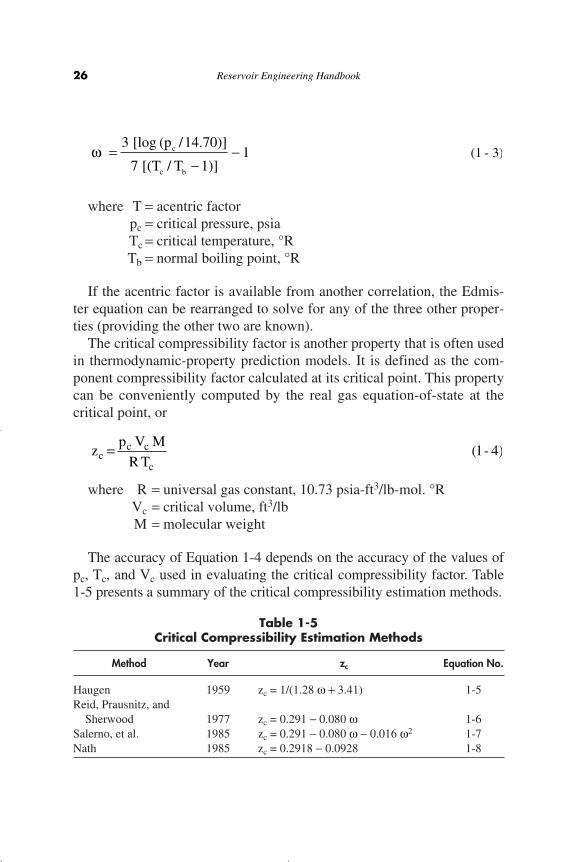
where T = acentric factorpc = critical pressure, psiaTc = critical temperature, °RTb = normal boiling point, °R
If the acentric factor is available from another correlation, the Edmis-ter equation can be rearranged to solve for any of the three other proper-ties (providing the other two are known).
The critical compressibility factor is another property that is often usedin thermodynamic-property prediction models. It is defined as the com-ponent compressibility factor calculated at its critical point. This propertycan be conveniently computed by the real gas equation-of-state at thecritical point, or
where R = universal gas constant, 10.73 psia-ft3/lb-mol. °RVc = critical volume, ft3/lbM = molecular weight
The accuracy of Equation 1-4 depends on the accuracy of the values ofpc, Tc, and Vc used in evaluating the critical compressibility factor. Table1-5 presents a summary of the critical compressibility estimation methods.
Table 1-5Critical Compressibility Estimation Methods
Method Year zc Equation No.
Haugen 1959 zc = 1/(1.28 w + 3.41) 1-5Reid, Prausnitz, and
Sherwood 1977 zc = 0.291 - 0.080 w 1-6Salerno, et al. 1985 zc = 0.291 - 0.080 w - 0.016 w2 1-7Nath 1985 zc = 0.2918 - 0.0928 1-8
zp V M
R Tcc c
c= (1- 4)
w =-
-3 [log (p /14.70)]
7 [(T / T 1)]1c
c b
(1 - 3)
26 Reservoir Engineering Handbook
Reservoir Eng Hndbk Ch 01 2001-10-24 09:04 Page 26

Example 1-1
Estimate the critical properties and the acentric factor of the heptanes-plus fraction, i.e., C7+, with a measured molecular weight of 150 and spe-cific gravity of 0.78.
Solution
Step 1. Use Equation 1-2 to estimate Tc, pc, Vc, and Tb:
• Tc = 544.2 (150).2998 (.78)1.0555 exp[-1.3478 ¥ 10-4 (150) -0.61641 (.78) + 0] = 1139.4 °R
• pc = 4.5203 ¥ 104 (150)–.8063 (.78)1.6015 exp[–1.8078 ¥ 10-3
(150) - 0.3084 (.78) + 0] =320.3 psia• Vc = 1.206 ¥ 10-2 (150).20378 (.78)-1.3036 exp[–2.657 ¥ 10-3
(150) + 0.5287 (.78) = 2.6012 ¥ 10-3 (150) (.78)] = .06035 ft3/lb• Tb = 6.77857 (150).401673 (.78)-1.58262 exp[3.77409 ¥ 10-3 (150)
+ 2.984036 (0.78) - 4.25288 ¥ 10-3 (150) (0.78)] = 825.26 °R
Step 2. Use Edmister’s Equation (Equation 1-3) to estimate the acentricfactor:
PROBLEMS
1. The following is a list of the compositional analysis of different hydro-carbon systems. The compositions are expressed in the terms of mol%.
Component System #1 System #2 System #3 System #4
C1 68.00 25.07 60.00 12.15C2 9.68 11.67 8.15 3.10C3 5.34 9.36 4.85 2.51C4 3.48 6.00 3.12 2.61C5 1.78 3.98 1.41 2.78C6 1.73 3.26 2.47 4.85C7+ 9.99 40.66 20.00 72.00
Classify these hydrocarbon systems.
w = [ ]-[ ] - =
3 320 3 14 7
7 1139 4 825 26 11 0 5067
log( . / . )
. / ..
Fundamentals of Reservoir Fluid Behavior 27
Reservoir Eng Hndbk Ch 01 2001-10-24 09:04 Page 27

2. If a petroleum fraction has a measured molecular weight of 190 and aspecific gravity of 0.8762, characterize this fraction by calculating theboiling point, critical temperature, critical pressure, and critical vol-ume of the fraction. Use the Riazi and Daubert correlation.
3. Calculate the acentric factor and critical compressibility factor of thecomponent in the above problem.
REFERENCES
1. Ahmed, T., “Composition Modeling of Tyler and Mission Canyon FormationOils with CO2 and Lean Gases,” final report submitted to the Montana’s on aNew Track for Science (MONTS) program (Montana National Science Foun-dation Grant Program), 1985.
2. Edmister, W. C., “Applied Hydrocarbon Thermodynamic, Part 4: Compress-ibility Factors and Equations of State,” Petroleum Refiner, April 1958, Vol.37, pp. 173–179.
3. Haugen, O. A., Watson, K. M., and Ragatz R. A., Chemical Process Princi-ples, 2nd ed. New York: Wiley, 1959, p. 577.
4. Katz, D. L. and Firoozabadi, A., “Predicting Phase Behavior ofCondensate/Crude-oil Systems Using Methane Interaction Coefficients,” JPT,Nov. 1978, pp. 1649–1655.
5. McCain, W. D., “Heavy Components Control Reservoir Fluid Behavior,”JPT, September 1994, pp. 746–750.
6. Nath, J., “Acentric Factor and Critical Volumes for Normal Fluids,” Ind. Eng.Chem. Fundam., 1985, Vol. 21, No. 3, pp. 325–326.
7. Reid, R., Prausnitz, J. M., and Sherwood, T., The Properties of Gases andLiquids, 3rd ed., pp. 21. McGraw-Hill, 1977.
8. Riazi, M. R. and Daubert, T. E., “Characterization Parameters for PetroleumFractions,” Ind. Eng. Chem. Res., 1987, Vol. 26, No. 24, pp. 755–759.
9. Salerno, S., et al., “Prediction of Vapor Pressures and Saturated Vol.,” FluidPhase Equilibria, June 10, 1985, Vol. 27, pp. 15–34.
28 Reservoir Engineering Handbook
Reservoir Eng Hndbk Ch 01 2001-10-24 09:04 Page 28

To understand and predict the volumetric behavior of oil and gas reser-voirs as a function of pressure, knowledge of the physical properties ofreservoir fluids must be gained. These fluid properties are usually deter-mined by laboratory experiments performed on samples of actual reser-voir fluids. In the absence of experimentally measured properties, it isnecessary for the petroleum engineer to determine the properties fromempirically derived correlations. The objective of this chapter is to pre-sent several of the well-established physical property correlations for thefollowing reservoir fluids:
• Natural gases• Crude oil systems• Reservoir water systems
PROPERTIES OF NATURAL GASES
A gas is defined as a homogeneous fluid of low viscosity and densitythat has no definite volume but expands to completely fill the vessel inwhich it is placed. Generally, the natural gas is a mixture of hydrocarbonand nonhydrocarbon gases. The hydrocarbon gases that are normallyfound in a natural gas are methanes, ethanes, propanes, butanes, pentanes,and small amounts of hexanes and heavier. The nonhydrocarbon gases(i.e., impurities) include carbon dioxide, hydrogen sulfide, and nitrogen.
29
C H A P T E R 2
RESERVOIR-FLUIDPROPERTIES
Reservoir Eng Hndbk Ch 02a 2001-10-24 09:23 Page 29
Knowledge of pressure-volume-temperature (PVT) relationships andother physical and chemical properties of gases is essential for solvingproblems in natural gas reservoir engineering. These properties include:
• Apparent molecular weight, Ma
• Specific gravity, gg
• Compressibility factor, z• Density, rg
• Specific volume, v• Isothermal gas compressibility coefficient, cg
• Gas formation volume factor, Bg
• Gas expansion factor, Eg
• Viscosity, mg
The above gas properties may be obtained from direct laboratory mea-surements or by prediction from generalized mathematical expressions.This section reviews laws that describe the volumetric behavior of gasesin terms of pressure and temperature and also documents the mathemati-cal correlations that are widely used in determining the physical proper-ties of natural gases.
BEHAVIOR OF IDEAL GASES
The kinetic theory of gases postulates that gases are composed of avery large number of particles called molecules. For an ideal gas, the vol-ume of these molecules is insignificant compared with the total volumeoccupied by the gas. It is also assumed that these molecules have noattractive or repulsive forces between them, and that all collisions ofmolecules are perfectly elastic.
Based on the above kinetic theory of gases, a mathematical equationcalled equation-of-state can be derived to express the relationship exist-ing between pressure p, volume V, and temperature T for a given quantityof moles of gas n. This relationship for perfect gases is called the idealgas law and is expressed mathematically by the following equation:
pV = nRT (2 - 1)
where p = absolute pressure, psiaV = volume, ft3
T = absolute temperature, °R
30 Reservoir Engineering Handbook
Reservoir Eng Hndbk Ch 02a 2001-10-24 09:23 Page 30
n = number of moles of gas, lb-moleR = the universal gas constant which, for the above units, has the
value 10.730 psia ft3/lb-mole °R
The number of pound-moles of gas, i.e., n, is defined as the weight ofthe gas m divided by the molecular weight M, or:
Combining Equation 2-1 with 2-2 gives:
where m = weight of gas, lbM = molecular weight, lb/lb-mol
Since the density is defined as the mass per unit volume of the sub-stance, Equation 2-3 can be rearranged to estimate the gas density at anypressure and temperature:
where rg = density of the gas, lb/ft3
It should be pointed out that lb refers to lbs mass in any of the subse-quent discussions of density in this text.
Example 2-1
Three pounds of n-butane are placed in a vessel at 120°F and 60 psia.Calculate the volume of the gas assuming an ideal gas behavior.
Solution
Step 1. Determine the molecular weight of n-butane from Table 1-1 to give:
M = 58.123
rgmV
pMRT
= = (2 - 4)
pVmM
RT= ÊË
ˆ¯ (2 - 3)
nmM
= (2 - 2)
Reservoir-Fluid Properties 31
Reservoir Eng Hndbk Ch 02a 2001-10-24 09:23 Page 31
Step 2. Solve Equation 2-3 for the volume of gas:
Example 2-2
Using the data given in the above example, calculate the density n-butane.
Solution
Solve for the density by applying Equation 2-4:
Petroleum engineers are usually interested in the behavior of mixturesand rarely deal with pure component gases. Because natural gas is a mix-ture of hydrocarbon components, the overall physical and chemical prop-erties can be determined from the physical properties of the individualcomponents in the mixture by using appropriate mixing rules.
The basic properties of gases are commonly expressed in terms of theapparent molecular weight, standard volume, density, specific volume,and specific gravity. These properties are defined as follows:
Apparent Molecular Weight
One of the main gas properties that is frequently of interest to engi-neers is the apparent molecular weight. If yi represents the mole fractionof the ith component in a gas mixture, the apparent molecular weight isdefined mathematically by the following equation:
where Ma = apparent molecular weight of a gas mixtureMi = molecular weight of the ith component in the mixtureyi = mole fraction of component i in the mixture
M y Ma i ii
==
Â1
2 5( )-
rg lb ft= =( ) ( . )( . ) ( )
. /60 58 12310 73 580
0 56 3
VmM
RTp
V ft
= ÊË
ˆ¯
= ÊË
ˆ¯
+ =358 123
10 73 120 46060
5 35 3
.( . ) ( )
.
32 Reservoir Engineering Handbook
Reservoir Eng Hndbk Ch 02a 2001-10-24 09:23 Page 32
Standard Volume
In many natural gas engineering calculations, it is convenient to mea-sure the volume occupied by l lb-mole of gas at a reference pressure andtemperature. These reference conditions are usually 14.7 psia and 60°F,and are commonly referred to as standard conditions. The standard vol-ume is then defined as the volume of gas occupied by 1 lb-mol of gas atstandard conditions. Applying the above conditions to Equation 2-1 andsolving for the volume, i.e., the standard volume, gives:
or
Vsc = 379.4 scf/lb-mol (2 - 6)
where Vsc = standard volume, scf/lb-molscf = standard cubic feetTsc = standard temperature, °Rpsc = standard pressure, psia
Density
The density of an ideal gas mixture is calculated by simply replacingthe molecular weight of the pure component in Equation 2-4 with theapparent molecular weight of the gas mixture to give:
where rg = density of the gas mixture, lb/ft3
Ma = apparent molecular weight
Specific Volume
The specific volume is defined as the volume occupied by a unit massof the gas. For an ideal gas, this property can be calculated by applyingEquation 2-3:
vVm
RTp Ma g
= = = 1r
(2 - 8)
rgapM
RT= (2 - 7)
VRT
pscsc
sc= =( ) ( ) ( . ) ( )
.1 1 10 73 520
14 7
Reservoir-Fluid Properties 33
Reservoir Eng Hndbk Ch 02a 2001-10-24 09:23 Page 33

where v = specific volume, ft3/lbrg = gas density, lb/ft3
Specific Gravity
The specific gravity is defined as the ratio of the gas density to that ofthe air. Both densities are measured or expressed at the same pressureand temperature. Commonly, the standard pressure psc and standard tem-perature Tsc are used in defining the gas specific gravity:
Assuming that the behavior of both the gas mixture and the air isdescribed by the ideal gas equation, the specific gravity can then beexpressed as:
or
where gg = gas specific gravityrair = density of the air
Mair = apparent molecular weight of the air = 28.96Ma = apparent molecular weight of the gaspsc = standard pressure, psiaTsc = standard temperature, °R
Example 2-3
A gas well is producing gas with a specific gravity of 0.65 at a rate of1.1 MMscf/day. The average reservoir pressure and temperature are1,500 psi and 150°F. Calculate:
a. Apparent molecular weight of the gasb. Gas density at reservoir conditionsc. Flow rate in lb/day
g ga
air
aMM
M= =28 96.
(2 -10)
g g
sc a
sc
sc air
sc
p MRT
p MRT
=
gr
rgg
air= (2 - 9)
34 Reservoir Engineering Handbook
Reservoir Eng Hndbk Ch 02a 2001-10-24 09:23 Page 34

Solution
a. From Equation 2-10, solve for the apparent molecular weight:
Ma = 28.96 gg
Ma = (28.96) (0.65) = 18.82
b. Apply Equation 2-7 to determine gas density:
c. Step 1. Because 1 lb-mol of any gas occupies 379.4 scf at standardconditions, then the daily number of moles that the gas wellis producing can be calculated from:
Step 2. Determine the daily mass m of the gas produced from Equa-tion 2-2:
m = (n) (Ma)
m = (2899) (18.82) = 54559 lb/day
Example 2-4
A gas well is producing a natural gas with the following composition:
Component yi
CO2 0.05C1 0.90C2 0.03C3 0.02
n lb mol= =( . ) ( ).
1 1 10379 4
28996
-
rg lb ft= =( ) ( . )( . ) ( )
. /1500 18 8210 73 610
4 31 3
Reservoir-Fluid Properties 35
Reservoir Eng Hndbk Ch 02a 2001-10-24 09:23 Page 35

Assuming an ideal gas behavior, calculate:
a. Apparent molecular weightb. Specific gravityc. Gas density at 2000 psia and 150°Fd. Specific volume at 2000 psia and 150°F
Solution
Component yi M i yi • Mi
CO2 0.05 44.01 2.200C1 0.90 16.04 14.436C2 0.03 30.07 0.902C3 0.02 44.11 0.882
Ma = 18.42
a. Apply Equation 2-5 to calculate the apparent molecular weight:
Ma = 18.42
b. Calculate the specific gravity by using Equation 2-10:
gg = 18.42 / 28.96 = 0.636
c. Solve for the density by applying Equation 2-7:
d. Determine the specific volume from Equation 2-8:
BEHAVIOR OF REAL GASES
In dealing with gases at a very low pressure, the ideal gas relationshipis a convenient and generally satisfactory tool. At higher pressures, theuse of the ideal gas equation-of-state may lead to errors as great as 500%,as compared to errors of 2–3% at atmospheric pressure.
v ft lb= =15 628
0 178 3
.. /
rg lb ft= =( ) ( . )( . ) ( )
. /2000 18 4210 73 610
5 628 3
36 Reservoir Engineering Handbook
Reservoir Eng Hndbk Ch 02a 2001-10-24 09:23 Page 36

Basically, the magnitude of deviations of real gases from the condi-tions of the ideal gas law increases with increasing pressure and tempera-ture and varies widely with the composition of the gas. Real gasesbehave differently than ideal gases. The reason for this is that the perfectgas law was derived under the assumption that the volume of moleculesis insignificant and that no molecular attraction or repulsion existsbetween them. This is not the case for real gases.
Numerous equations-of-state have been developed in the attempt tocorrelate the pressure-volume-temperature variables for real gases withexperimental data. In order to express a more exact relationship betweenthe variables p, V, and T, a correction factor called the gas compressibili-ty factor, gas deviation factor, or simply the z-factor, must be introducedinto Equation 2-1 to account for the departure of gases from ideality. Theequation has the following form:
pV = znRT (2-11)
where the gas compressibility factor z is a dimensionless quantity and isdefined as the ratio of the actual volume of n-moles of gas at T and p tothe ideal volume of the same number of moles at the same T and p:
Studies of the gas compressibility factors for natural gases of variouscompositions have shown that compressibility factors can be generalizedwith sufficient accuracies for most engineering purposes when they areexpressed in terms of the following two dimensionless properties:
• Pseudo-reduced pressure• Pseudo-reduced temperature
These dimensionless terms are defined by the following expressions:
TT
Tprpc
= (2 -13)
pp
pprpc
= (2 -12)
zVV
VnRT p
actual
ideal= =
( ) /
Reservoir-Fluid Properties 37
Reservoir Eng Hndbk Ch 02a 2001-10-24 09:23 Page 37
where p = system pressure, psiappr = pseudo-reduced pressure, dimensionlessT = system temperature, °R
Tpr = pseudo-reduced temperature, dimensionlessppc, Tpc = pseudo-critical pressure and temperature, respectively, and
defined by the following relationships:
It should be pointed out that these pseudo-critical properties, i.e., ppc
and Tpc, do not represent the actual critical properties of the gas mixture.These pseudo properties are used as correlating parameters in generatinggas properties.
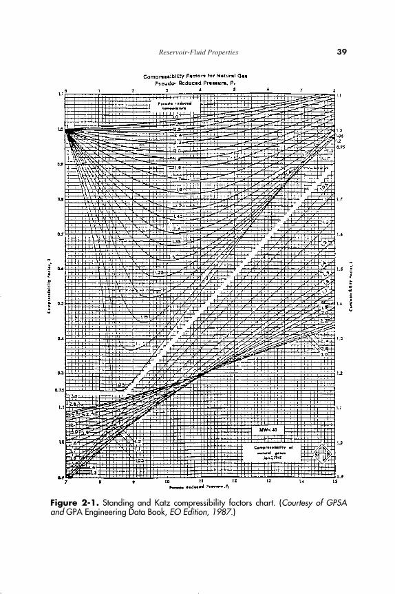
Based on the concept of pseudo-reduced properties, Standing and Katz(1942) presented a generalized gas compressibility factor chart as shownin Figure 2-1. The chart represents compressibility factors of sweet natur-al gas as a function of ppr and Tpr. This chart is generally reliable for nat-ural gas with minor amount of nonhydrocarbons. It is one of the mostwidely accepted correlations in the oil and gas industry.
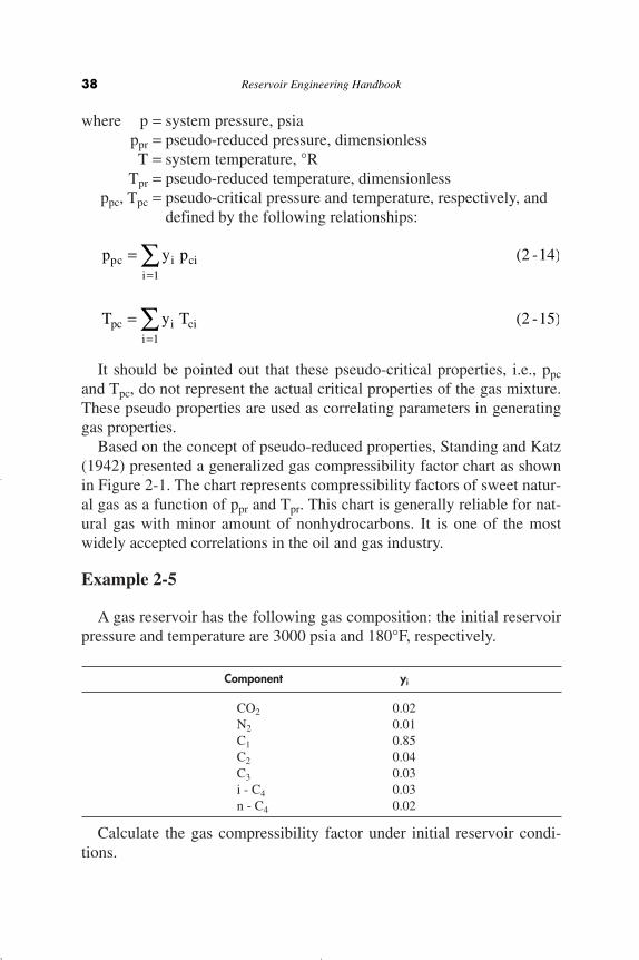
Example 2-5
A gas reservoir has the following gas composition: the initial reservoirpressure and temperature are 3000 psia and 180°F, respectively.
Component yi
CO2 0.02N2 0.01C1 0.85C2 0.04C3 0.03i - C4 0.03n - C4 0.02
Calculate the gas compressibility factor under initial reservoir condi-tions.
T y Tpc i cii
==
Â1
(2 -15)
p y ppc i cii
==
Â1
(2 -14)
38 Reservoir Engineering Handbook
Reservoir Eng Hndbk Ch 02a 2001-10-24 09:23 Page 38
Reservoir-Fluid Properties 39
Figure 2-1. Standing and Katz compressibility factors chart. (Courtesy of GPSAand GPA Engineering Data Book, EO Edition, 1987.)
Reservoir Eng Hndbk Ch 02a 2001-10-24 09:23 Page 39
Solution
Component yi Tci,°R yiTci pci yi pci
CO2 0.02 547.91 10.96 1071 21.42N2 0.01 227.49 2.27 493.1 4.93C1 0.85 343.33 291.83 666.4 566.44C2 0.04 549.92 22.00 706.5 28.26C3 0.03 666.06 19.98 616.4 18.48i - C4 0.03 734.46 22.03 527.9 15.84n - C4 0.02 765.62 15.31 550.6 11.01
Tpc = 383.38 ppc = 666.38
Step 1. Determine the pseudo-critical pressure from Equation 2-14:
ppc = 666.18
Step 2. Calculate the pseudo-critical temperature from Equation 2-15:
Tpc = 383.38
Step 3. Calculate the pseudo-reduced pressure and temperature by apply-ing Equations 2-12 and 2-13, respectively:
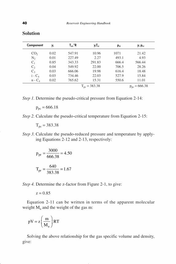
Step 4. Determine the z-factor from Figure 2-1, to give:
z = 0.85
Equation 2-11 can be written in terms of the apparent molecularweight Ma and the weight of the gas m:
Solving the above relationship for the gas specific volume and density,give:
pV zm
MRT
a=
ÊËÁ
ˆ¯
p
T
pr
pr
= =
= =
3000666 38
4 50
640383 38
1 67
..
..
40 Reservoir Engineering Handbook
Reservoir Eng Hndbk Ch 02a 2001-10-24 09:23 Page 40

where v = specific volume, ft3/lbrg = density, lb/ft3
Example 2-6
Using the data in Example 2-5 and assuming real gas behavior, calcu-late the density of the gas phase under initial reservoir conditions. Com-pare the results with that of ideal gas behavior.
Solution
Component yi Mi yi • Mi Tci,°R yiTci pci yi pci
CO2 0.02 44.01 0.88 547.91 10.96 1071 21.42N2 0.01 28.01 0.28 227.49 2.27 493.1 4.93C1 0.85 16.04 13.63 343.33 291.83 666.4 566.44C2 0.04 30.1 1.20 549.92 22.00 706.5 28.26C3 0.03 44.1 1.32 666.06 19.98 616.40 18.48i - C4 0.03 58.1 1.74 734.46 22.03 527.9 15.84n - C4 0.02 58.1 1.16 765.62 15.31 550.6 11.01
Ma = 20.23 Tpc = 383.38 Ppc = 666.38
Step 1. Calculate the apparent molecular weight from Equation 2-5:
Ma = 20.23
Step 2. Determine the pseudo-critical pressure from Equation 2-14:
ppc = 666.18
Step 3. Calculate the pseudo-critical temperature from Equation 2-15:
Tpc = 383.38
Step 4. Calculate the pseudo-reduced pressure and temperature by apply-ing Equations 2-12 and 2-13, respectively:
rga
vpMzRT
= =1(2 -17)
vVm
zRTpMa
= = (2 -16)
Reservoir-Fluid Properties 41
Reservoir Eng Hndbk Ch 02a 2001-10-24 09:23 Page 41
Step 5. Determine the z-factor from Figure 2-1:
z = 0.85
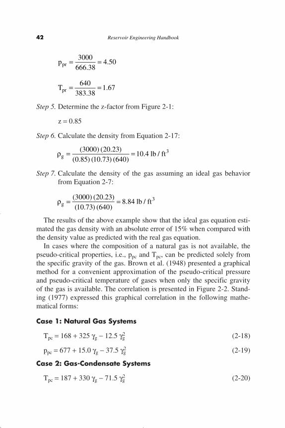
Step 6. Calculate the density from Equation 2-17:
Step 7. Calculate the density of the gas assuming an ideal gas behaviorfrom Equation 2-7:
The results of the above example show that the ideal gas equation esti-mated the gas density with an absolute error of 15% when compared withthe density value as predicted with the real gas equation.
In cases where the composition of a natural gas is not available, thepseudo-critical properties, i.e., ppc and Tpc, can be predicted solely fromthe specific gravity of the gas. Brown et al. (1948) presented a graphicalmethod for a convenient approximation of the pseudo-critical pressureand pseudo-critical temperature of gases when only the specific gravityof the gas is available. The correlation is presented in Figure 2-2. Stand-ing (1977) expressed this graphical correlation in the following mathe-matical forms:
Case 1: Natural Gas Systems
Tpc = 168 + 325 gg - 12.5 gg2 (2-18)
ppc = 677 + 15.0 gg - 37.5 gg2 (2-19)
Case 2: Gas-Condensate Systems
Tpc = 187 + 330 gg - 71.5 gg2 (2-20)
rg lb ft= =( ) ( . )( . ) ( )
. /3000 20 2310 73 640
8 84 3
rg lb ft= =( ) ( . )( . ) ( . ) ( )
. /3000 20 23
0 85 10 73 64010 4 3
p
T
pr
pr
= =
= =
3000666 38
4 50
640383 38
1 67
..
..
42 Reservoir Engineering Handbook
Reservoir Eng Hndbk Ch 02a 2001-10-24 09:23 Page 42
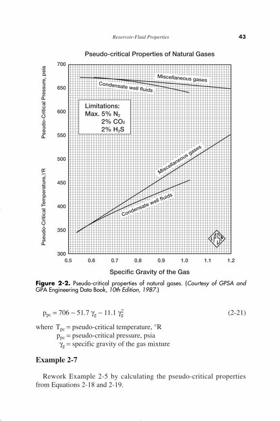
ppc = 706 - 51.7 gg - 11.1 gg2 (2-21)
where Tpc = pseudo-critical temperature, °Rppc = pseudo-critical pressure, psia
gg = specific gravity of the gas mixture
Example 2-7
Rework Example 2-5 by calculating the pseudo-critical propertiesfrom Equations 2-18 and 2-19.
Reservoir-Fluid Properties 43
3000.5
350
400
450
500
550
600
650
700
0.6 0.7 0.8 0.9
Specific Gravity of the Gas
Pseudo-critical Properties of Natural Gases
Pse
udo
-Cri
tical
Tem
per
atur
e,°R
Pse
udo
-Cri
tical
Pre
ssur
e, p
sia
1.0 1.1 1.2
Miscellaneous gases
Miscellaneous gases
Condensate well fluids
Condensate well fluids
Limitations:Max. 5% N2
2% CO2
2% H2S
Figure 2-2. Pseudo-critical properties of natural gases. (Courtesy of GPSA andGPA Engineering Data Book, 10th Edition, 1987.)
Reservoir Eng Hndbk Ch 02a 2001-10-24 09:23 Page 43

Solution
Step 1. Calculate the specific gravity of the gas:
Step 2. Solve for the pseudo-critical properties by applying Equations2-18 and 2-19:
Tpc = 168 + 325 (0.699) - 12.5 (0.699)2 = 389.1°R
ppc = 677 + 15 (0.699) - 37.5 (0.699)2 = 669.2 psia
Step 3. Calculate ppr and Tpr.
Step 4. Determine the gas compressibility factor from Figure 2-1:
z = 0.824
Step 5. Calculate the density from Equation 2-17:
EFFECT OF NONHYDROCARBON COMPONENTSON THE Z-FACTOR
Natural gases frequently contain materials other than hydrocarboncomponents, such as nitrogen, carbon dioxide, and hydrogen sulfide.Hydrocarbon gases are classified as sweet or sour depending on thehydrogen sulfide content. Both sweet and sour gases may contain nitro-gen, carbon dioxide, or both. A hydrocarbon gas is termed a sour gas if itcontains one grain of H2S per 100 cubic feet.
The common occurrence of small percentages of nitrogen and carbondioxide is, in part, considered in the correlations previously cited. Con-
rg lb ft= =( ) ( . )( . ) ( . ) ( )
. /3000 20 23
0 845 10 73 64010 46 3
p
T
pr
pr
= =
= =
3000669 2
4 48
640389 1
1 64
..
..
g gaM= = =
28 9620 2328 96
0 699.
.
..
44 Reservoir Engineering Handbook
Reservoir Eng Hndbk Ch 02a 2001-10-24 09:23 Page 44

centrations of up to 5 percent of these nonhydrocarbon components willnot seriously affect accuracy. Errors in compressibility factor calculationsas large as 10 percent may occur in higher concentrations of nonhydro-carbon components in gas mixtures.
Nonhydrocarbon Adjustment Methods
There are two methods that were developed to adjust the pseudo-criti-cal properties of the gases to account for the presence of the nonhydro-carbon components. These two methods are the:
• Wichert-Aziz correction method• Carr-Kobayashi-Burrows correction method
The Wichert-Aziz Correction Method
Natural gases that contain H2S and or CO2 frequently exhibit differentcompressibility-factors behavior than do sweet gases. Wichert and Aziz(1972) developed a simple, easy-to-use calculation procedure to accountfor these differences. This method permits the use of the Standing-Katzchart, i.e., Figure 2-1, by using a pseudo-critical temperature adjustmentfactor, which is a function of the concentration of CO2 and H2S in thesour gas. This correction factor is then used to adjust the pseudo-criticaltemperature and pressure according to the following expressions:
T¢pc = Tpc - e (2 - 22)
where Tpc = pseudo-critical temperature, °Rppc = pseudo-critical pressure, psiaT¢pc = corrected pseudo-critical temperature, °Rp¢pc = corrected pseudo-critical pressure, psia
B = mole fraction of H2S in the gas mixturee = pseudo-critical temperature adjustment factor and is defined
mathematically by the following expression
e = 120 [A0.9 - A1.6] + 15 (B0.5 - B4.0) (2 - 24)
where the coefficient A is the sum of the mole fraction H2S and CO2 inthe gas mixture, or:
¢ =¢
+ -p
p T
T B Bpcpc pc
pc ( )1 e(2 - 23)
Reservoir-Fluid Properties 45
Reservoir Eng Hndbk Ch 02a 2001-10-24 09:23 Page 45

A = yH2S + yCO2
The computational steps of incorporating the adjustment factor e intothe z-factor calculations are summarized below:
Step 1. Calculate the pseudo-critical properties of the whole gas mixtureby applying Equations 2-18 and 2-19 or Equations 2-20 and 2-21.
Step 2. Calculate the adjustment factor e from Equation 2-24.
Step 3. Adjust the calculated ppc and Tpc (as computed in Step 1) byapplying Equations 2-22 and 2-23.
Step 4. Calculate the pseudo-reduced properties, i.e., ppr and Tpr, fromEquations 2-11 and 2-12.
Step 5. Read the compressibility factor from Figure 2-1.
Example 2-8
A sour natural gas has a specific gravity of 0.7. The compositionalanalysis of the gas shows that it contains 5 percent CO2 and 10 percentH2S. Calculate the density of the gas at 3500 psia and 160°F.
Solution
Step 1. Calculate the uncorrected pseudo-critical properties of the gasfrom Equations 2-18 and 2-19:
Tpc = 168 + 325 (0.7) - 12.5 (0.7)2 = 389.38°R
ppc = 677 + 15 (0.7) - 37.5 (0.7)2 = 669.1 psia
Step 2. Calculate the pseudo-critical temperature adjustment factor fromEquation 2-24:
e = 120 (0.150.9 - 0.151.6) + 15 (0.10.5 - 0.14) = 20.735
Step 3. Calculate the corrected pseudo-critical temperature by applyingEquation 2-22:
46 Reservoir Engineering Handbook
Reservoir Eng Hndbk Ch 02a 2001-10-24 09:23 Page 46
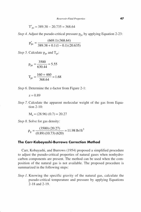
T¢pc = 389.38 - 20.735 = 368.64
Step 4. Adjust the pseudo-critical pressure ppc by applying Equation 2-23:
Step 5. Calculate ppr and Tpr:
Step 6. Determine the z-factor from Figure 2-1:
z = 0.89
Step 7. Calculate the apparent molecular weight of the gas from Equa-tion 2-10:
Ma = (28.96) (0.7) = 20.27
Step 8. Solve for gas density:
The Carr-Kobayashi-Burrows Correction Method
Carr, Kobayashi, and Burrows (1954) proposed a simplified procedureto adjust the pseudo-critical properties of natural gases when nonhydro-carbon components are present. The method can be used when the com-position of the natural gas is not available. The proposed procedure issummarized in the following steps:
Step 1. Knowing the specific gravity of the natural gas, calculate thepseudo-critical temperature and pressure by applying Equations2-18 and 2-19.
rg lb ft= =( ) ( . )( . ) ( . ) ( )
. /3500 20 27
0 89 10 73 62011 98 3
p
T
pr
pr
= =
= + =
3500630 44
5 55
160 460368 64
1 68
..
..
¢ =+ -
ppc( . ) ( . )
. . ( . ) ( . )669 1 368 64
389 38 0 1 1 0 1 20 635
Reservoir-Fluid Properties 47
Reservoir Eng Hndbk Ch 02a 2001-10-24 09:23 Page 47

Step 2. Adjust the estimated pseudo-critical properties by using the fol-lowing two expressions:
T¢pc = Tpc - 80 yCO2 + 130 yH2S - 250 yN2 (2-25)
p¢pc = ppc + 440 yCO2 + 600 yH2S - 170 yN2 (2-26)
where T¢pc = the adjusted pseudo-critical temperature, °RTpc = the unadjusted pseudo-critical temperature, °R
yCO2 = mole fraction of CO2
yN2 = mole fraction of H2S in the gas mixture= mole fraction of Nitrogen
p¢pc = the adjusted pseudo-critical pressure, psiappc = the unadjusted pseudo-critical pressure, psia
Step 3. Use the adjusted pseudo-critical temperature and pressure to cal-culate the pseudo-reduced properties.
Step 4. Calculate the z-factor from Figure 2-1.
Example 2-9
Using the data in Example 2-8, calculate the density by employing theabove correction procedure.
Solution
Step 1. Determine the corrected pseudo-critical properties from Equa-tions 2-25 and 2-26:
T¢pc = 389.38 - 80 (0.05) + 130 (0.10) - 250 (0) = 398.38°R
p¢pc = 669.1 + 440 (0.05) + 600 (0.10) - 170 (0) = 751.1 psia
Step 2. Calculate ppr and Tpr:
p
T
pr
pr
= =
= =
3500751 1
4 56
620398 38
1 56
..
..
48 Reservoir Engineering Handbook
Reservoir Eng Hndbk Ch 02a 2001-10-24 09:23 Page 48

Step 3. Determine the gas compressibility factor from Figure 2-1:
z = 0.820
Step 4. Calculate the gas density:
CORRECTION FOR HIGH-MOLECULARWEIGHT GASES
It should be noted that the Standing and Katz compressibility factorchart (Figure 2-1) was prepared from data on binary mixtures of methanewith propane, ethane, and butane, and on natural gases, thus covering awide range in composition of hydrocarbon mixtures containing methane.No mixtures having molecular weights in excess of 40 were included inpreparing this plot.
Sutton (1985) evaluated the accuracy of the Standing-Katz compress-ibility factor chart using laboratory-measured gas compositions and z-factors, and found that the chart provides satisfactory accuracy for engi-neering calculations. However, Kay’s mixing rules, i.e., Equations 2-13and 2-14 (or comparable gravity relationships for calculating pseudo-crit-ical pressure and temperature), result in unsatisfactory z-factors for highmolecular weight reservoir gases. The author observed that large devia-tions occur to gases with high heptanes-plus concentrations. He pointedout that Kay’s mixing rules should not be used to determine the pseudo-critical pressure and temperature for reservoir gases with specific gravi-ties greater than about 0.75.
Sutton proposed that this deviation can be minimized by utilizing themixing rules developed by Stewart et al. (1959), together with newlyintroduced empirical adjustment factors (FJ, EJ, and EK) that are relatedto the presence of the heptane-plus fraction in the gas mixture. The pro-posed approach is outlined in the following steps:
Step 1. Calculate the parameters J and K from the following relationships:
J y T p y T pi ci cii
i ci cii
=È
ÎÍÍ
˘
˚˙˙
+È
ÎÍÍ
˘
˚˙˙
 Â13
23
0 5
2
( / ) ( / ) . (2 - 27)
rg lb ft= =( ) ( . )( . ) ( . ) ( )
. /3500 20 27
0 82 10 73 62013 0 3
Reservoir-Fluid Properties 49
Reservoir Eng Hndbk Ch 02a 2001-10-24 09:23 Page 49

where J = Stewart-Burkhardt-Voo correlating parameter, °R/psiaK = Stewart-Burkhardt-Voo correlating parameter, °R/psiayi = mole fraction of component i in the gas mixture.
Step 2. Calculate the adjustment parameters FJ, EJ, and EK from the fol-lowing expressions:
EJ = 0.6081 FJ + 1.1325 F2J - 14.004 FJ yC7+
+ 64.434 FJ y2C7+ (2 - 30)
EK = [Tc/M pc]C7+ [0.3129 yC7+ - 4.8156 (yC7+)2
+ 27.3751 (yC7+)3] (2 - 31)
where yC7+ = mole fraction of the heptanes-plus component(Tc)C7+ = critical temperature of the C7+(pc)C7+ = critical pressure of the C7+
Step 3. Adjust the parameters J and K by applying the adjustment factorsEJ and EK, according to the relationships:
J¢ = J - EJ (2 - 32)
K¢ = K - EK (2 - 33)
where J, K = calculated from Equations 2-27 and 2-28EJ, EK = calculated from Equations 2-30 and 2-31
Step 4. Calculate the adjusted pseudo-critical temperature and pressurefrom the expressions:
¢ =¢¢
pT
Jpcpc (2 - 35)
¢ = ¢¢
TKJpc
( )2
(2 - 34)
F y T p y T pJ c c C c c C= ++ +13
237
0 57
2[ ( / )] [ ( / ) ]. (2 - 29)
K y T pi ci cii
= Â[ / ] (2 - 28)
50 Reservoir Engineering Handbook
Reservoir Eng Hndbk Ch 02a 2001-10-24 09:23 Page 50
Step 5. Having calculated the adjusted Tpc and ppc, the regular procedureof calculating the compressibility factor from the Standing andKatz chart is followed.
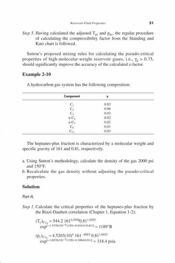
Sutton’s proposed mixing rules for calculating the pseudo-criticalproperties of high-molecular-weight reservoir gases, i.e., gg > 0.75,should significantly improve the accuracy of the calculated z-factor.
Example 2-10
A hydrocarbon gas system has the following composition:
Component y
C1 0.83C2 0.06C3 0.03
n-C4 0.02n-C5 0.02C6 0.01C7+ 0.03
The heptanes-plus fraction is characterized by a molecular weight andspecific gravity of 161 and 0.81, respectively.
a. Using Sutton’s methodology, calculate the density of the gas 2000 psiand 150°F.
b. Recalculate the gas density without adjusting the pseudo-criticalproperties.
Solution
Part A.
Step 1. Calculate the critical properties of the heptanes-plus fraction bythe Riazi-Daubert correlation (Chapter 1, Equation 1-2):
(Tc)C7+ = 544.2 1610.29980.811.0555
exp[-1.3478(10)-4(150)-0.61641(0.81)] = 1189°R
(pc)C7+ = 4.5203(10)4 161-.8063 0.811.6015
exp[-1.8078(10)-3(150)-0.3084(0.81)] = 318.4 psia
Reservoir-Fluid Properties 51
Reservoir Eng Hndbk Ch 02a 2001-10-24 09:23 Page 51
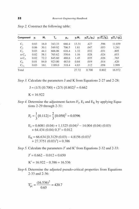
Step 2. Construct the following table:
Component yi Mi Tci pci yiM i yi(Tci/pci) yiZ(Tc/pc)i yi[Tc/Zpc]i
C1 0.83 16.0 343.33 666.4 13.31 .427 .596 11.039C2 0.06 30.1 549.92 706.5 1.81 .047 .053 1.241C3 0.03 44.1 666.06 616.4 1.32 .032 .031 .805n-C4 0.02 58.1 765.62 550.6 1.16 .028 .024 .653n-C5 0.02 72.2 845.60 488.6 1.45 .035 .026 .765C6 0.01 84.0 923.00 483.0 0.84 .019 .014 .420C7+ 0.03 161. 1189.0 318.4 4.83 .112 .058 1.999
Total 27.72 0.700 0.802 16.972
Step 3. Calculate the parameters J and K from Equations 2-27 and 2-28:
J = (1/3) [0.700] + (2/3) [0.802]2 = 0.662
K = 16.922
Step 4. Determine the adjustment factors FJ, EJ and EK by applying Equa-tions 2-29 through 2-31:
EJ = 0.6081 (0.04) + 1.1325 (0.04)2 - 14.004 (0.04) (0.03)+ 64.434 (0.04) 0.32 = 0.012
EK = 66.634 [0.3129 (0.03) - 4.8156 (0.03)2
+ 27.3751 (0.03)3] = 0.386
Step 5. Calculate the parameters J¢ and K¢ from Equations 2-32 and 2-33:
J¢ = 0.662 - 0.012 = 0.650
K¢ = 16.922 - 0.386 = 16.536
Step 6. Determine the adjusted pseudo-critical properties from Equations2-33 and 2-36:
¢ = =Tpc( . )
..
16 5360 65
420 72
FJ = + =13
0 11223
0 058 0 03962[ . ] [ . ] .
52 Reservoir Engineering Handbook
Reservoir Eng Hndbk Ch 02a 2001-10-24 09:23 Page 52

Step 7. Calculate the pseudo-reduced properties of the gas by applyingEquations 2-11 and 2-12, to give:
Step 8. Calculate the z-factor from Figure 2-1, to give:
z = 0.745
Step 9. From Equation 2-16, calculate the density of the gas:
Part B.
Step 1. Calculate the specific gravity of the gas:
Step 2. Solve for the pseudo-critical properties by applying Equations2-18 and 2-19:
Tpc = 168 + 325 (0.854) - 12.5 (0.854)2 = 436.4°R
ppc = 677 + 15 (0.854) - 37.5 (0.854)2 = 662.5 psia
Step 3. Calculate ppr and Tpr:
p
T
pr
pr
= =
= =
2000662 5
3 02
610436 4
1 40
..
..
g gaM= = =
28 9624 7328 96
0 854.
.
..
rg lb ft= =( ) ( . )( . ) ( ) (. )
. /2000 24 73
10 73 610 74510 14 3
p
T
pr
pr
= =
= =
2000647 2
3 09
610420 7
1 45
..
..
¢ = =ppc420 70 65
647 2.
..
Reservoir-Fluid Properties 53
Reservoir Eng Hndbk Ch 02a 2001-10-24 09:23 Page 53

Step 4. Calculate the z-factor from Figure 2-1, to give:
z = 0.710
Step 5. From Equation 2-16, calculate the density of the gas:
DIRECT CALCULATION OFCOMPRESSIBILITY FACTORS
After four decades of existence, the Standing-Katz z-factor chart isstill widely used as a practical source of natural gas compressibility fac-tors. As a result, there has been an apparent need for a simple mathemati-cal description of that chart. Several empirical correlations for calculat-ing z-factors have been developed over the years. The following threeempirical correlations are described below:
• Hall-Yarborough• Dranchuk-Abu-Kassem• Dranchuk-Purvis-Robinson
The Hall-Yarborough Method
Hall and Yarborough (1973) presented an equation-of-state that accu-rately represents the Standing and Katz z-factor chart. The proposedexpression is based on the Starling-Carnahan equation-of-state. The coef-ficients of the correlation were determined by fitting them to data takenfrom the Standing and Katz z-factor chart. Hall and Yarborough proposedthe following mathematical form:
where ppr = pseudo-reduced pressuret = reciprocal of the pseudo-reduced temperature, i.e., Tpc/T
Y = the reduced density that can be obtained as the solution ofthe following equation:
zp t
Ytpr= È
Î͢˚
- -0 06125
1 2 1 2.exp [ . ( ) ] (2 - 36)
rg lb ft= =( ) ( . )( . ) ( ) (. )
. /2000 24 73
10 73 610 71010 64 3
54 Reservoir Engineering Handbook
Reservoir Eng Hndbk Ch 02a 2001-10-24 09:23 Page 54

where X1 = -0.06125 ppr t exp [-1.2 (1 - t)2]X2 = (14.76 t - 9.76 t2 + 4.58 t3)X3 = (90.7 t - 242.2 t2 + 42.4 t3)X4 = (2.18 + 2.82 t)
Equation 2-37 is a nonlinear equation and can be conveniently solvedfor the reduced density Y by using the Newton-Raphson iteration tech-nique. The computational procedure of solving Equation 2-37 at anyspecified pseudo-reduced pressure ppr and temperature Tpr is summarizedin the following steps:
Step 1. Make an initial guess of the unknown parameter, Yk, where k isan iteration counter. An appropriate initial guess of Y is given bythe following relationship:
Yk = 0.0125 ppr t exp [-1.2 (1 - t)2]
Step 2. Substitute this initial value in Equation 2-37 and evaluate thenonlinear function. Unless the correct value of Y has been initial-ly selected, Equation 2-37 will have a nonzero value of F(Y):
Step 3. A new improved estimate of Y, i.e., Yk+1, is calculated from thefollowing expression:
where f¢(Yk) is obtained by evaluating the derivative of Equation2-37 at Yk, or:
Step 4. Steps 2–3 are repeated n times, until the error, i.e., abs(Yk -Yk+1), becomes smaller than a preset tolerance, e.g., 10-12:
¢ = + + - +-
-
+ -
f YY Y Y Y
YX Y
X X Y X
( )( )
( )
( ) ( ) ( )
1 4 4 4
12 2
3 4
2 3 4
4
4 1 (2 - 39)
Y Yf Y
f Yk k
k
k+ = -
¢1 ( )
( )(2 - 38)
F Y XY Y Y Y
YX Y X YX( )
( )( ) ( )= + + + +
-- + =1
12 3 0
2 3 4
32 4 (2 - 37)
Reservoir-Fluid Properties 55
Reservoir Eng Hndbk Ch 02a 2001-10-24 09:23 Page 55
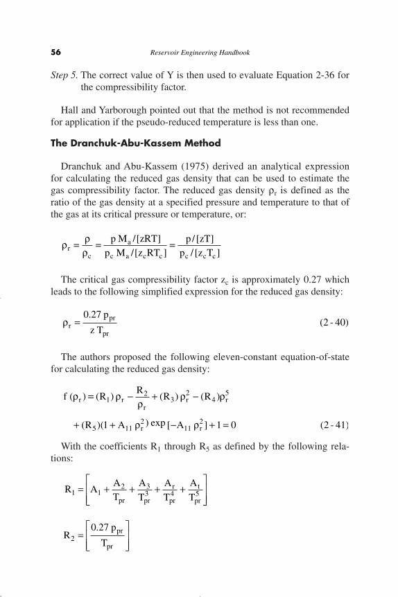
Step 5. The correct value of Y is then used to evaluate Equation 2-36 forthe compressibility factor.
Hall and Yarborough pointed out that the method is not recommendedfor application if the pseudo-reduced temperature is less than one.
The Dranchuk-Abu-Kassem Method
Dranchuk and Abu-Kassem (1975) derived an analytical expressionfor calculating the reduced gas density that can be used to estimate thegas compressibility factor. The reduced gas density rr is defined as theratio of the gas density at a specified pressure and temperature to that ofthe gas at its critical pressure or temperature, or:
The critical gas compressibility factor zc is approximately 0.27 whichleads to the following simplified expression for the reduced gas density:
The authors proposed the following eleven-constant equation-of-statefor calculating the reduced gas density:
With the coefficients R1 through R5 as defined by the following rela-tions:
R AAT
A
T
A
T
A
T
Rp
T
pr pr
r
pr
t
pr
pr
pr
1 12 3
3 4 5
2
0 27
= + + + +È
ÎÍÍ
˘
˚˙˙
=È
ÎÍÍ
˘
˚˙˙
.
f RR
R R
R A A
r rr
r r
r r
( ) ( ) ( ) ( )
( )( ) exp [ ] (
r rr
r r
r r
= - + -
+ + - + =
12
32
45
5 112
1121 1 0 2 - 41)
rrpr
pr
p
z T=
0 27.(2 - 40)
r rrr
c
a
c a c c c c c
p M zRTp M z RT
p zTp z T
= = =/[ ]/[ ]
/ [ ]/ [ ]
56 Reservoir Engineering Handbook
Reservoir Eng Hndbk Ch 02a 2001-10-24 09:23 Page 56
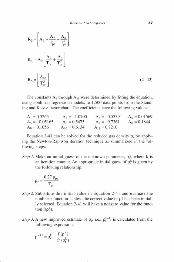
The constants A1 through A11 were determined by fitting the equation,using nonlinear regression models, to 1,500 data points from the Stand-ing and Katz z-factor chart. The coefficients have the following values:
A1 = 0.3265 A2 = -1.0700 A3 = -0.5339 A4 = 0.01569A5 = -0.05165 A6 = 0.5475 A7 = -0.7361 A8 = 0.1844A9 = 0.1056 A10 = 0.6134 A11 = 0.7210
Equation 2-41 can be solved for the reduced gas density rr by apply-ing the Newton-Raphson iteration technique as summarized in the fol-lowing steps:
Step 1. Make an initial guess of the unknown parameter, r rk, where k is
an iteration counter. An appropriate initial guess of rrk is given by
the following relationship:
Step 2. Substitute this initial value in Equation 2-41 and evaluate thenonlinear function. Unless the correct value of rr
k has been initial-ly selected, Equation 2-41 will have a nonzero value for the func-tion f(rr
k).
Step 3. A new improved estimate of rr, i.e., rrk+1, is calculated from the
following expression:
r r rrr
krk r
k
rk
f
f+ = -
¢1 ( )
( )
rrpr
pr
p
T=
0 27.
R AAT
A
T
R AAT
A
T
RA
T
pr pr
pr pr
pr
3 67 8
2
4 97 8
2
5103
= + +È
ÎÍÍ
˘
˚˙˙
= +È
ÎÍÍ
˘
˚˙˙
=È
ÎÍÍ
˘
˚˙˙
(2 - 42)
Reservoir-Fluid Properties 57
Reservoir Eng Hndbk Ch 02a 2001-10-24 09:23 Page 57

where
Step 4. Steps 2–3 are repeated n times, until the error, i.e., abs(r rk - rr
k+1),becomes smaller than a preset tolerance, e.g., 10-12.
Step 5. The correct value of rr is then used to evaluate Equation 2-40 forthe compressibility factor, i.e.,:
The proposed correlation was reported to duplicate compress-ibility factors from the Standing and Katz chart with an averageabsolute error of 0.585 percent and is applicable over the ranges:
0.2 ≤ ppr < 30
1.0 < Tpr ≤ 3.0
The Dranchuk-Purvis-Robinson Method
Dranchuk, Purvis, and Robinson (1974) developed a correlation basedon the Benedict-Webb-Rubin type of equation-of-state. Fitting the equa-tion to 1,500 data points from the Standing and Katz z-factor chart opti-mized the eight coefficients of the proposed equations. The equation hasthe following form:
with
1 12
pr
3
pr3T = A + A
T+ A
T
È
ÎÍ
˘
˚˙
1 + T + T + T + [T (1 A )
( A )] T = 0
1 r 2 r2
3 r5
4 r2
8 r2
8 r2 5
r
r r r r r
rr
+
- -exp (2 - 43)
zp
Tpr
r pr=
0 27.
r
¢ = + + - +
- + - +
f RR
R R R
A A A A
rr
r r r
r r r r
( ) ( ) ( ) ( ) ( )
exp [ ][( ) ( )]
rr
r r r
r r r r
122 3 4
45
112
113
112
112
2 5 2
1 2 1
58 Reservoir Engineering Handbook
Reservoir Eng Hndbk Ch 02a 2001-10-24 09:23 Page 58
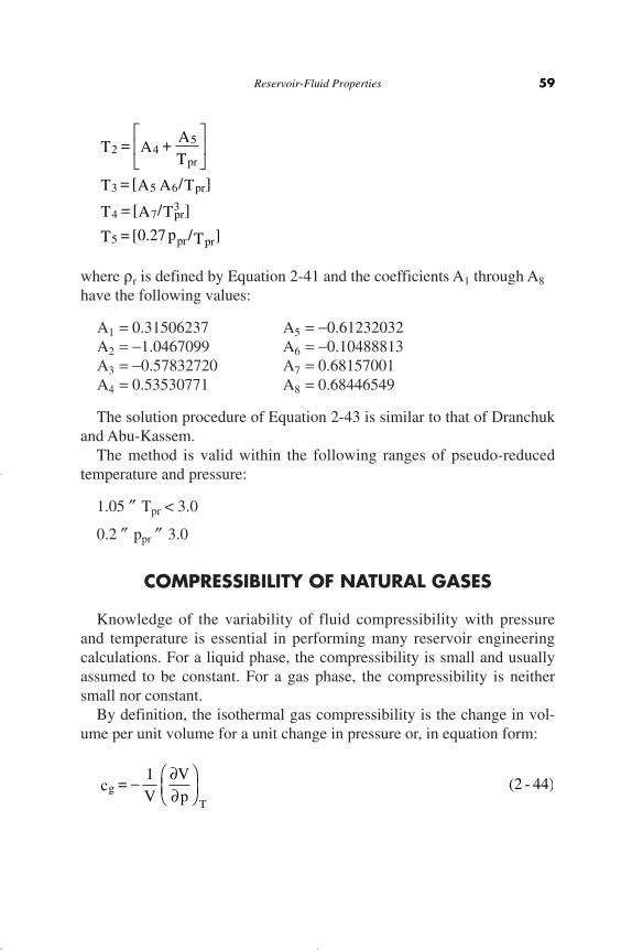
where rr is defined by Equation 2-41 and the coefficients A1 through A8
have the following values:
A1 = 0.31506237 A5 = -0.61232032A2 = -1.0467099 A6 = -0.10488813A3 = -0.57832720 A7 = 0.68157001A4 = 0.53530771 A8 = 0.68446549
The solution procedure of Equation 2-43 is similar to that of Dranchukand Abu-Kassem.
The method is valid within the following ranges of pseudo-reducedtemperature and pressure:
1.05 ≤ Tpr < 3.0
0.2 ≤ ppr ≤ 3.0
COMPRESSIBILITY OF NATURAL GASES
Knowledge of the variability of fluid compressibility with pressureand temperature is essential in performing many reservoir engineeringcalculations. For a liquid phase, the compressibility is small and usuallyassumed to be constant. For a gas phase, the compressibility is neithersmall nor constant.
By definition, the isothermal gas compressibility is the change in vol-ume per unit volume for a unit change in pressure or, in equation form:
gT
c =1V
Vp
- ∂∂
ÊËÁ
ˆ¯
(2 - 44)
2 45
pr
3 5 6 pr
4 7 pr3
5 pr pr
T = A + AT
T = [A A /T ]
T = [A /T ]
T = [0.27 p /T ]
È
ÎÍ
˘
˚˙
Reservoir-Fluid Properties 59
Reservoir Eng Hndbk Ch 02a 2001-10-24 09:23 Page 59

where cg = isothermal gas compressibility, 1/psi.
From the real gas equation-of-state:
Differentiating the above equation with respect to pressure at constanttemperature T gives:
Substituting into Equation 2-44 produces the following generalizedrelationship:
For an ideal gas, z = 1 and (∂z/∂p)T = 0, therefore:
It should be pointed out that Equation 2-46 is useful in determining theexpected order of magnitude of the isothermal gas compressibility.
Equation 2-45 can be conveniently expressed in terms of the pseudo-reduced pressure and temperature by simply replacing p with (ppc ppr), or:
Multiplying the above equation by ppc yields:
g pc prpr pr Tpr
c p = c =1
p1z
zp
- ∂∂
È
ÎÍÍ
˘
˚˙˙
(2 - 47)
gpr pc
prTpr pcc =
1p p
1z
z (p p
- ∂∂
È
ÎÍÍ
˘
˚˙˙)
gc =1p
(2 - 46)
gT
c =1p
1z
zp
- ∂∂
ÊËÁ
ˆ¯
(2 - 45)
∂∂
ÊËÁ
ˆ¯
∂∂
ÊËÁ
ˆ¯
-È
ÎÍ
˘
˚˙
Vp
= nRT1p
zp
zp
T2
V =nRTz
p
60 Reservoir Engineering Handbook
Reservoir Eng Hndbk Ch 02a 2001-10-24 09:23 Page 60
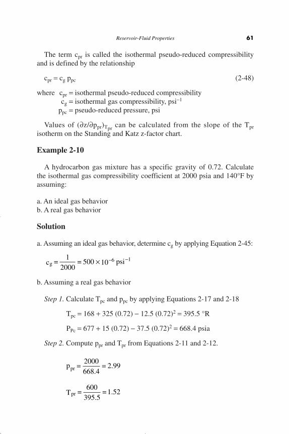
The term cpr is called the isothermal pseudo-reduced compressibilityand is defined by the relationship
cpr = cg ppc (2-48)
where cpr = isothermal pseudo-reduced compressibilitycg = isothermal gas compressibility, psi-1
ppc = pseudo-reduced pressure, psi
Values of (∂z/∂ppr)Tpr can be calculated from the slope of the Tpr
isotherm on the Standing and Katz z-factor chart.
Example 2-10
A hydrocarbon gas mixture has a specific gravity of 0.72. Calculatethe isothermal gas compressibility coefficient at 2000 psia and 140°F byassuming:
a. An ideal gas behaviorb. A real gas behavior
Solution
a. Assuming an ideal gas behavior, determine cg by applying Equation 2-45:
b. Assuming a real gas behavior
Step 1. Calculate Tpc and ppc by applying Equations 2-17 and 2-18
Tpc = 168 + 325 (0.72) - 12.5 (0.72)2 = 395.5 °R
PPc = 677 + 15 (0.72) - 37.5 (0.72)2 = 668.4 psia
Step 2. Compute ppr and Tpr from Equations 2-11 and 2-12.
pr
pr
p =2000668.4
= 2.99
T =600
395.5= 1.52
g6 1c =
12000
= 500 10 psi¥ - -
Reservoir-Fluid Properties 61
Reservoir Eng Hndbk Ch 02a 2001-10-24 09:23 Page 61
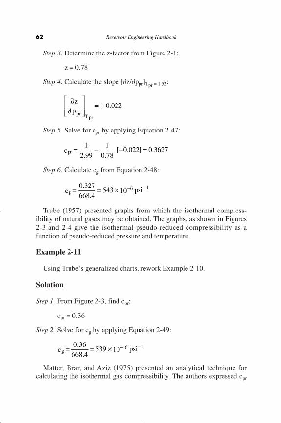
Step 3. Determine the z-factor from Figure 2-1:
z = 0.78
Step 4. Calculate the slope [∂z/∂ppr]Tpr = 1.52:
Step 5. Solve for cpr by applying Equation 2-47:
Step 6. Calculate cg from Equation 2-48:
Trube (1957) presented graphs from which the isothermal compress-ibility of natural gases may be obtained. The graphs, as shown in Figures2-3 and 2-4 give the isothermal pseudo-reduced compressibility as afunction of pseudo-reduced pressure and temperature.
Example 2-11
Using Trube’s generalized charts, rework Example 2-10.
Solution
Step 1. From Figure 2-3, find cpr:
cpr = 0.36
Step 2. Solve for cg by applying Equation 2-49:
Matter, Brar, and Aziz (1975) presented an analytical technique forcalculating the isothermal gas compressibility. The authors expressed cpr
g 6 1c =
0.36668.4
= 539 10 psi¥ - -
g6 1c =
0.327668.4
= 543 10 psi¥ - -
prc =1
2.991
0.78 [ 0.022] = 0.3627- -
prTpr
zp
= 0.022∂
∂
È
ÎÍÍ
˘
˚˙˙
-
62 Reservoir Engineering Handbook
Reservoir Eng Hndbk Ch 02a 2001-10-24 09:23 Page 62
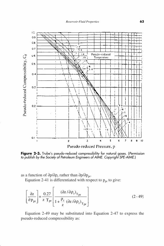
as a function of ∂p/∂rr rather than ∂p/∂ppr.Equation 2-41 is differentiated with respect to ppr to give:
Equation 2-49 may be substituted into Equation 2-47 to express thepseudo-reduced compressibility as:
∂∂
È
ÎÍÍ
˘
˚˙˙
∂ ∂
∂ ∂
È
Î
ÍÍÍ
˘
˚
˙˙˙
zp
=0.27z T
( z / )
1 +z
( z / )pr pr
prTr
rprTr
r
r r(2 - 49)
Reservoir-Fluid Properties 63
Figure 2-3. Trube’s pseudo-reduced compressibility for natural gases. (Permissionto publish by the Society of Petroleum Engineers of AIME. Copyright SPE-AIME.)
Reservoir Eng Hndbk Ch 02a 2001-10-24 09:23 Page 63
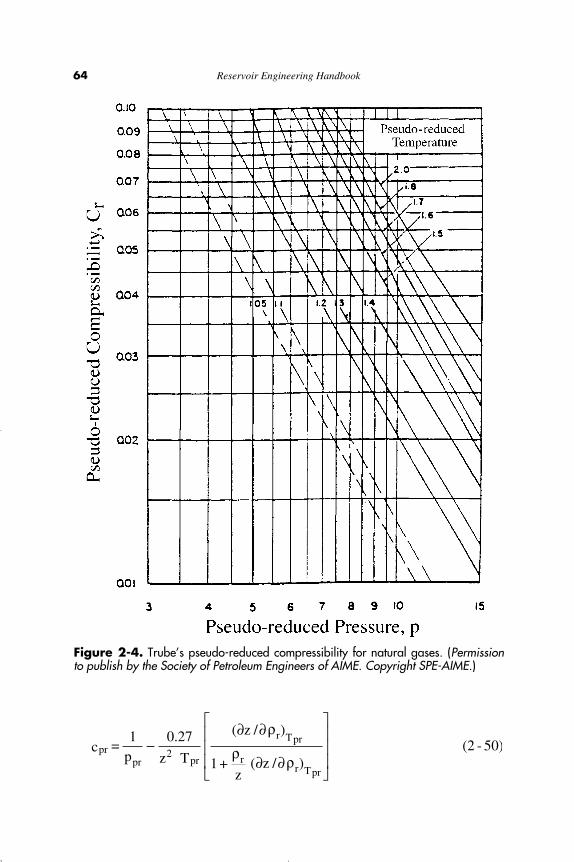
prpr
2pr
prTr
rprTr
c =1
p0.27
z T
( z / )
1 +z
( z / )-
∂ ∂
∂ ∂
È
Î
ÍÍÍ
˘
˚
˙˙˙
r
r r(2 - 50)
64 Reservoir Engineering Handbook
Figure 2-4. Trube’s pseudo-reduced compressibility for natural gases. (Permissionto publish by the Society of Petroleum Engineers of AIME. Copyright SPE-AIME.)
Reservoir Eng Hndbk Ch 02a 2001-10-24 09:23 Page 64

where rr = pseudo-reduced gas density.
The partial derivative appearing in Equation 2-50 is obtained fromEquation 2-43 to give:
where the coefficients T1 through T4 and A1 through A8 are definedpreviously by Equation 2-43.
GAS FORMATION VOLUME FACTOR
The gas formation volume factor is used to relate the volume of gas, asmeasured at reservoir conditions, to the volume of the gas as measured atstandard conditions, i.e., 60°F and 14.7 psia. This gas property is thendefined as the actual volume occupied by a certain amount of gas at aspecified pressure and temperature, divided by the volume occupied bythe same amount of gas at standard conditions. In an equation form, therelationship is expressed as
where Bg = gas formation volume factor, ft3/scfVp,T = volume of gas at pressure p and temperature, T, ft3
Vsc = volume of gas at standard conditions, scf
Applying the real gas equation-of-state, i.e., Equation 2-11, and substi-tuting for the volume V, gives:
where zsc = z-factor at standard conditions = 1.0psc, Tsc = standard pressure and temperature
gsc sc
sc
sc
scB =
zn RTp
z n R Tp
=p
TzTp
gp,T
scB =
V
V(2 - 52)
∂∂
È
ÎÍ
˘
˚˙ -
¥ -
z= T + 2 T + 5 T + 2 T (1 + A A )
( A )
r Tpr
1 2 r 3 r4
4 r 8 r2
82
r4
8 r2
rr r r r r
rexp (2 - 51)
Reservoir-Fluid Properties 65
Reservoir Eng Hndbk Ch 02a 2001-10-24 09:23 Page 65
Assuming that the standard conditions are represented by psc =14.7psia and Tsc = 520, the above expression can be reduced to the followingrelationship:
where Bg = gas formation volume factor, ft3/scfz = gas compressibility factorT = temperature, °R
In other field units, the gas formation volume factor can be expressedin bbl/scf, to give:
The reciprocal of the gas formation volume factor is called the gasexpansion factor and is designated by the symbol Eg, or:
In other units:
Example 2-12
A gas well is producing at a rate of 15,000 ft3/day from a gas reservoirat an average pressure of 2,000 psia and a temperature of 120°F. The spe-cific gravity is 0.72. Calculate the gas flow rate in scf/day.
Solution
Step 1. Calculate the pseudo-critical properties from Equations 2-17 and2-18, to give:
TPc = 395.5 °R ppc = 668.4 psia
gE = 198.6p
zT, scf /bbl (2 - 56)
gE = 35.37p
zT, scf / ft3 (2 - 55)
Bz Tpg = 0 005035. (2 - 54)
Bz Tpg = 0 02827. (2 - 53)
66 Reservoir Engineering Handbook
Reservoir Eng Hndbk Ch 02a 2001-10-24 09:23 Page 66

Step 2. Calculate the ppr and Tpr:
Step 3. Determine the z-factor from Figure 2-1:
z = 0.78
Step 4. Calculate the gas expansion factor from Equation 2-55:
Step 5. Calculate the gas flow rate in scf/day by multiplying the gas flowrate (in ft3/day) by the gas expansion factor Eg as expressed inscf/ft3:
Gas flow rate = (151.15) (15,000) = 2.267 MMscf/day
GAS VISCOSITY
The viscosity of a fluid is a measure of the internal fluid friction (resis-tance) to flow. If the friction between layers of the fluid is small, i.e., lowviscosity, an applied shearing force will result in a large velocity gradi-ent. As the viscosity increases, each fluid layer exerts a larger frictionaldrag on the adjacent layers and velocity gradient decreases.
The viscosity of a fluid is generally defined as the ratio of the shearforce per unit area to the local velocity gradient. Viscosities areexpressed in terms of poises, centipoise, or micropoises. One poiseequals a viscosity of 1 dyne-sec/cm2 and can be converted to other fieldunits by the following relationships:
1 poise = 100 centipoises= 1 ¥ 106 micropoises= 6.72 ¥ 10-2 lb mass/ft-sec= 2.09 ¥ 10-3 lb-sec/ft2
gE = 35.372000
(0.78) (600)= 151.15 scf /ft3
pr
pr
p =2000668.4
= 2.99
T =600
395.5= 1.52
Reservoir-Fluid Properties 67
Reservoir Eng Hndbk Ch 02a 2001-10-24 09:23 Page 67
The gas viscosity is not commonly measured in the laboratory becauseit can be estimated precisely from empirical correlations. Like all inten-sive properties, viscosity of a natural gas is completely described by thefollowing function:
mg = (p,T,yi)
where mg = the viscosity of the gas phase. The above relationship simplystates that the viscosity is a function of pressure, temperature, and com-position. Many of the widely used gas viscosity correlations may beviewed as modifications of that expression.
METHODS OF CALCULATING THE VISCOSITY OFNATURAL GASES
Two popular methods that are commonly used in the petroleum indus-try are the:
• Carr-Kobayashi-Burrows Correlation Method• Lee-Gonzalez-Eakin Method
The Carr-Kobayashi-Burrows Correlation Method
Carr, Kobayashi, and Burrows (1954) developed graphical correlationsfor estimating the viscosity of natural gas as a function of temperature,pressure, and gas gravity. The computational procedure of applying theproposed correlations is summarized in the following steps:
Step 1. Calculate the pseudo-critical pressure, pseudo-critical tempera-ture, and apparent molecular weight from the specific gravity orthe composition of the natural gas. Corrections to these pseudo-critical properties for the presence of the nonhydrocarbon gases(CO2, N2, and H2S) should be made if they are present in concen-trations greater than 5 mole percent.
Step 2. Obtain the viscosity of the natural gas at one atmosphere and thetemperature of interest from Figure 2-5. This viscosity, as denotedby m1, must be corrected for the presence of nonhydrocarboncomponents by using the inserts of Figure 2-5. The nonhydrocar-bon fractions tend to increase the viscosity of the gas phase. Theeffect of nonhydrocarbon components on the viscosity of the nat-
68 Reservoir Engineering Handbook
Reservoir Eng Hndbk Ch 02a 2001-10-24 09:23 Page 68

Reservoir-F
luid Properties
69
Figure 2-5. Carr’s atmospheric gas viscosity correlation. (Permission to publish by the Society of Petroleum Engineers of AIME. Copy-right SPE-AIME.)
Reservoir Eng Hndbk Ch 02a 2
001-10-24 0
9:23 P
age 69

ural gas can be expressed mathematically by the following rela-tionships:
m1 = (m1)uncorrected + (Dm)N2 + (Dm)CO2 + (Dm)H2S (2-57)
where m1 = “corrected” gas viscosity at one atmosphericpressure and reservoir temperature, cp
(Dm)N2 = viscosity corrections due to the presence of N2
(Dm)CO2 = viscosity corrections due to the presence of CO2
(Dm)H2S = viscosity corrections due to the presence of H2S(m1)uncorrected = uncorrected gas viscosity, cp
Step 3. Calculate the pseudo-reduced pressure and temperature.
Step 4. From the pseudo-reduced temperature and pressure, obtain theviscosity ratio (mg/m1) from Figure 2-6. The term mg represents theviscosity of the gas at the required conditions.
Step 5. The gas viscosity, mg, at the pressure and temperature of interestis calculated by multiplying the viscosity at one atmosphere andsystem temperature, m1, by the viscosity ratio.
The following examples illustrate the use of the proposed graphicalcorrelations:
Example 2-13
Using the data given in Example 2-12, calculate the viscosity of the gas.
Solution
Step 1. Calculate the apparent molecular weight of the gas:
Ma = (0.72) (28.96) = 20.85
Step 2. Determine the viscosity of the gas at 1 atm and 140°F from Fig-ure 2-5:
m1 = 0.0113
70 Reservoir Engineering Handbook
Reservoir Eng Hndbk Ch 02a 2001-10-24 09:23 Page 70

Reservoir-F
luid Properties
71Figure 2-6. Carr’s viscosity ratio correlation. (Permission to publish by the Society of Petroleum Engineers of AIME. Copyright SPE-
AIME.)
Reservoir Eng Hndbk Ch 02a 2
001-10-24 0
9:23 P
age 71
Step 3. Calculate ppr and Tpr:
ppr = 2.99
Tpr = 1.52
Step 4. Determine the viscosity rates from Figure 2-6:
Step 5. Solve for the viscosity of the natural gas:
Standing (1977) proposed a convenient mathematical expression for cal-culating the viscosity of the natural gas at atmospheric pressure and reser-voir temperature, m1. Standing also presented equations for describing theeffects of N2, CO2, and H2S on m1. The proposed relationships are:
where:
where m1 = viscosity of the gas at atmospheric pressure andreservoir temperature, cp
T = reservoir temperature, °Rgg = gas gravity
yN2, yCO2, yH2S = mole fraction of N2, CO2, and H2S, respectively
Dempsey (1965) expressed the viscosity ratio mg/m1 by the followingrelationship:
H S H S g( ) = y [8.49 (10 ) ( ) + 3.73 (10 )]
2 23 3Dm g- -log (2 - 61)
( ) [ . ( ) log( ) . ( )]Dm gN N gy2 2
3 38 48 10 9 59 10= +- - (2 - 60)
( )co2Dm = ¥( ) + ¥( )[ ]- -yco g2
9 08 10 6 24 103 3. log .g
uncorrected1 g
g
( ) = [1.709 (10 2.062 10 ] (T 460)
+ 8.118 ( ) 6.15 (10 ) ( )
m g
g
- -
- -
- -
-
5 6
3 310 log (2 - 59)
1 uncorrected CO H S N= ( ) + ( ) + ( ) ( ) (2 - 58)
2 2 2m m m m m1 D D D+
gg
11= ( ) = (1.5) (0.0113) = 0.01695 cpm
mm
m
g
1
= 1.5mm
72 Reservoir Engineering Handbook
Reservoir Eng Hndbk Ch 02a 2001-10-24 09:23 Page 72

where Tpr = pseudo-reduced temperature of the gas mixture, °Rppr = pseudo-reduced pressure of the gas mixture, psia
a0 . . . a17 = coefficients of the equations are given below:
a0 = -2.46211820 a8 = -7.93385648 (10-1)a1 = 2.970547414 a9 = 1.39643306a2 = -2.86264054 (10-1) a10 = -1.49144925 (10-1)a3 = 8.05420522 (10-3) a11 = 4.41015512 (10-3)a4 = 2.80860949 a12 = 8.39387178 (10-2)a5 = -3.49803305 a13 = -1.86408848 (10-1)a6 = 3.60373020 (10-1) a14 = 2.03367881 (10-2)a7 = -1.044324 (10-2) a15 = -6.09579263 (10-4)
The Lee-Gonzalez-Eakin Method
Lee, Gonzalez, and Eakin (1966) presented a semi-empirical relation-ship for calculating the viscosity of natural gases. The authors expressedthe gas viscosity in terms of the reservoir temperature, gas density, andthe molecular weight of the gas. Their proposed equation is given by:
where
Y = 2.4 - 0.2 X (2 - 66)
X = 3.5 +986T
+ 0.01 Ma (2 - 65)
K =(9.4 + 0.02 M ) T
209 + 19 M + Ta
a
1 5.
(2 - 64)
gg
Y
= K Xmr
1062 4
4- ÊËÁ
ˆ¯
È
ÎÍÍ
˘
˚˙˙
exp.
(2 - 63)
ln
(
prg
1pr pr
23 pr
3pr pr
pr2
pr3
pr2
8 9 pr 10 pr2
11 pr3
pr3
12 13 pr 14 pr2
15 pr3
T = a + a p a p + a p + T (a + a p
+ a p a p ) + T (a + a p + a p + a p )
+ T a + a p + a p + a p )
mm
ÊËÁ
ˆ¯
È
ÎÍÍ
˘
˚˙˙
+
+
0 1 2 4 5
6 7
(2(2 - 62)
Reservoir-Fluid Properties 73
Reservoir Eng Hndbk Ch 02a 2001-10-24 09:23 Page 73
rg = gas density at reservoir pressure and temperature, lb/ft3
T = reservoir temperature, °RMa = apparent molecular weight of the gas mixture
The proposed correlation can predict viscosity values with a standarddeviation of 2.7% and a maximum deviation of 8.99%. The correlation isless accurate for gases with higher specific gravities. The authors pointedout that the method cannot be used for sour gases.
Example 2-14
Rework Example 2-13 and calculate the gas viscosity by using theLee-Gonzalez-Eakin method.
Step 1. Calculate the gas density from Equation 2-16:
Step 2. Solve for the parameters K, X, and Y by using Equations 2-64,2-65, and 2-66, respectively:
Step 3. Calculate the viscosity from Equation 2-63:
PROPERTIES OF CRUDE OIL SYSTEMS
Petroleum (an equivalent term is crude oil) is a complex mixture con-sisting predominantly of hydrocarbons and containing sulfur, nitrogen,oxygen, and helium as minor constituents. The physical and chemicalproperties of crude oils vary considerably and are dependent on the con-
g
1.33
= (119.72) 5.35 8.3
62.4= 0.0173 cpm 10 4- Ê
ˈ¯
È
ÎÍ
˘
˚˙exp
K =[9.4 + 0.02 (20.85)] (600)
209 + 19 (20.85) + 600= 119.72
X = 3.5 +986600
+ 0.01 (20.85) = 5.35
Y = 2.4 0.2 (5.35) = 1.33
1.5
-
g =(2000) (20.85)
(10.73) (600) (0.78)= 8.3 lb/ftr 3
74 Reservoir Engineering Handbook
Reservoir Eng Hndbk Ch 02a 2001-10-24 09:23 Page 74

centration of the various types of hydrocarbons and minor constituentspresent.
An accurate description of physical properties of crude oils is of a con-siderable importance in the fields of both applied and theoretical scienceand especially in the solution of petroleum reservoir engineering prob-lems. Physical properties of primary interest in petroleum engineeringstudies include:
• Fluid gravity• Specific gravity of the solution gas• Gas solubility• Bubble-point pressure• Oil formation volume factor• Isothermal compressibility coefficient of undersaturated crude oils• Oil density• Total formation volume factor• Crude oil viscosity• Surface tension
Data on most of these fluid properties are usually determined by labo-ratory experiments performed on samples of actual reservoir fluids. Inthe absence of experimentally measured properties of crude oils, it isnecessary for the petroleum engineer to determine the properties fromempirically derived correlations.
Crude Oil Gravity
The crude oil density is defined as the mass of a unit volume of thecrude at a specified pressure and temperature. It is usually expressed inpounds per cubic foot. The specific gravity of a crude oil is defined as theratio of the density of the oil to that of water. Both densities are measuredat 60°F and atmospheric pressure:
where go = specific gravity of the oilro = density of the crude oil, lb/ft3
rw = density of the water, lb/ft3
g rro
o
w= (2 - 67)
Reservoir-Fluid Properties 75
Reservoir Eng Hndbk Ch 02a 2001-10-24 09:23 Page 75
It should be pointed out that the liquid specific gravity is dimension-less, but traditionally is given the units 60°/60° to emphasize the fact thatboth densities are measured at standard conditions. The density of thewater is approximately 62.4 lb/ft3, or:
Although the density and specific gravity are used extensively in thepetroleum industry, the API gravity is the preferred gravity scale. Thisgravity scale is precisely related to the specific gravity by the followingexpression:
The API gravities of crude oils usually range from 47° API for thelighter crude oils to 10° API for the heavier asphaltic crude oils.
Example 2-15
Calculate the specific gravity and the API gravity of a crude oil systemwith a measured density of 53 lb/ft3 at standard conditions.
Solution
Step 1. Calculate the specific gravity from Equation 2-67:
Step 2. Solve for the API gravity:
Specific Gravity of the Solution Gas
The specific gravity of the solution gas gg is described by the weightedaverage of the specific gravities of the separated gas from each separator.
API = = API141 50 849
131 5 35 2.
.. .- ∞
g o = =53
62 40 849
..
∞ -API =o
141 5131 5
..
g(2 - 68)
g ro
o=62 4
60 60.
, /∞ ∞
76 Reservoir Engineering Handbook
Reservoir Eng Hndbk Ch 02a 2001-10-24 09:23 Page 76
This weighted-average approach is based on the separator gas-oil ratio,or:
where n = number of separatorsRsep = separator gas-oil ratio, scf/STB
gsep = separator gas gravityRst = gas-oil ratio from the stock tank, scf/ STB
gst = gas gravity from the stock tank
Example 2-16
Separator tests were conducted on a crude oil sample. Results of thetest in terms of the separator gas-oil ration and specific gravity of theseparated gas are given below:
Separator Pressure Temperature Gas-Oil Ratio Gas Specific# psig °F scf/STB Gravity
Primary 660 150 724 0.743Intermediate 75 110 202 0.956Stock tank 0 60 58 1.296
Calculate the specific gravity of the separated gas.
Solution
Estimate the specific gravity of the solution by using Equation 2-69:
Gas Solubility
The gas solubility Rs is defined as the number of standard cubic feet ofgas which will dissolve in one stock-tank barrel of crude oil at certain
g g = =( ) ( . ) ( ) ( . ) ( ) ( . )
.724 0 743 202 0 956 58 1 296
724 202 580 819
+ ++ +
gg g
g
sep i sep i st sti
n
sep i sti
n=
R R
R R
( ) ( )
( )
+
+
=
=
Â
Â1
1
(2 - 69)
Reservoir-Fluid Properties 77
Reservoir Eng Hndbk Ch 02a 2001-10-24 09:23 Page 77

pressure and temperature. The solubility of a natural gas in a crude oil is astrong function of the pressure, temperature, API gravity, and gas gravity.
For a particular gas and crude oil to exist at a constant temperature, thesolubility increases with pressure until the saturation pressure is reached.At the saturation pressure (bubble-point pressure) all the available gasesare dissolved in the oil and the gas solubility reaches its maximum value.Rather than measuring the amount of gas that will dissolve in a givenstock-tank crude oil as the pressure is increased, it is customary to deter-mine the amount of gas that will come out of a sample of reservoir crudeoil as pressure decreases.
A typical gas solubility curve, as a function of pressure for an under-saturated crude oil, is shown in Figure 2-7. As the pressure is reducedfrom the initial reservoir pressure pi, to the bubble-point pressure pb, nogas evolves from the oil and consequently the gas solubility remains con-stant at its maximum value of Rsb. Below the bubble-point pressure, thesolution gas is liberated and the value of Rs decreases with pressure. Thefollowing five empirical correlations for estimating the gas solubility aregiven below:
• Standing’s correlation• The Vasquez-Beggs correlation• Glaso’s correlation• Marhoun’s correlation• The Petrosky-Farshad correlation
Standing’s Correlation
Standing (1947) proposed a graphical correlation for determining thegas solubility as a function of pressure, gas specific gravity, API gravity,and system temperature. The correlation was developed from a total of105 experimentally determined data points on 22 hydrocarbon mixturesfrom California crude oils and natural gases. The proposed correlation hasan average error of 4.8%. Standing (1981) expressed his proposed graphi-cal correlation in the following more convenient mathematical form:
R =p
s gxg
18 21 4 10
1 2048
..
.
+ÊË
ˆ¯
ÈÎÍ
˘˚
(2 - 70)
78 Reservoir Engineering Handbook
Reservoir Eng Hndbk Ch 02a 2001-10-24 09:23 Page 78

with
x = 0.0125 API - 0.00091(T - 460)
where T = temperature, °Rp = system pressure, psia
gg = solution gas specific gravity
It should be noted that Standing’s equation is valid for applications atand below the bubble-point pressure of the crude oil.
Example 2-17
The following experimental PVT data on six different crude oil sys-tems are available. Results are based on two-stage surface separation.
Reservoir-Fluid Properties 79
Gas Solubility at pb
Pressure
Rsb
pb
Gas
Sol
ubili
ty R
s, s
cf/S
TB
Bub
ble-
poin
t Pre
ssur
e
Figure 2-7. Gas-solubility pressure diagram.
Reservoir Eng Hndbk Ch 02a 2001-10-24 09:23 Page 79

co atOil # T pb Rs Bo ro p > pb psep Tsep API gg
1 250 2377 751 1.528 38.13 22.14 ¥ 10-6 at 2689 150 60 47.1 0.8512 220 2620 768 1.474 40.95 18.75 ¥ 10-6 at 2810 100 75 40.7 0.8553 260 2051 693 1.529 37.37 22.69 ¥ 10-6 at 2526 100 72 48.6 0.9114 237 2884 968 1.619 38.92 21.51 ¥ 10-6 at 2942 60 120 40.5 0.8985 218 3045 943 1.570 37.70 24.16 ¥ 10-6 at 3273 200 60 44.2 0.7816 180 4239 807 1.385 46.79 11.45 ¥ 10-6 at 4370 85 173 27.3 0.848
where T = reservoir temperature, °Fpb = bubble-point pressure, psigBo = oil formation volume factor, bbl/STB
psep = separator pressure, psigTsep = separator temperature, °F
co = isothermal compressibility coefficient of the oil at aspecified pressure, psi-1
Using Standing’s correlation, estimate the gas solubility at the bubble-point pressure and compare with the experimental value in terms of theabsolute average error (AAE).
Solution
Apply Equation 2-70 to determine the gas solubility. Results of thecalculations are given in the following tabulated form:
Predicted RS Measured %Oil # X 10X Equation 2-70 RS Error
1 0.361 2.297 838 751 11.62 0.309 2.035 817 768 6.33 0.371 2.349 774 693 11.74 0.312 2.049 969 968 0.1085 0.322 2.097 1012 943 7.36 0.177 1.505 998 807 23.7
AAE = 10.1%
The Vasquez-Beggs Correlation
Vasquez and Beggs (1980) presented an improved empirical correla-tion for estimating Rs. The correlation was obtained by regression analy-
80 Reservoir Engineering Handbook
Reservoir Eng Hndbk Ch 02b 2001-10-24 09:26 Page 80
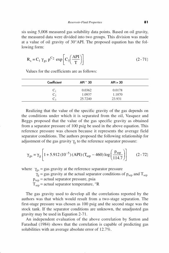
sis using 5,008 measured gas solubility data points. Based on oil gravity,the measured data were divided into two groups. This division was madeat a value of oil gravity of 30°API. The proposed equation has the fol-lowing form:
Values for the coefficients are as follows:
Coefficient API ≤ 30 API > 30
C1 0.0362 0.0178C2 1.0937 1.1870C3 25.7240 23.931
Realizing that the value of the specific gravity of the gas depends onthe conditions under which it is separated from the oil, Vasquez andBeggs proposed that the value of the gas specific gravity as obtainedfrom a separator pressure of 100 psig be used in the above equation. Thisreference pressure was chosen because it represents the average fieldseparator conditions. The authors proposed the following relationship foradjustment of the gas gravity gg to the reference separator pressure:
where ggs = gas gravity at the reference separator pressuregg = gas gravity at the actual separator conditions of psep and Tsep
psep = actual separator pressure, psiaTsep = actual separator temperature, °R
The gas gravity used to develop all the correlations reported by theauthors was that which would result from a two-stage separation. Thefirst-stage pressure was chosen as 100 psig and the second stage was thestock tank. If the separator conditions are unknown, the unadjusted gasgravity may be used in Equation 2-71.
An independent evaluation of the above correlation by Sutton andFarashad (1984) shows that the correlation is capable of predicting gassolubilities with an average absolute error of 12.7%.
g ggs g sepsep= API T
p1 5 912 10 460
114 75+ - Ê
ËÁˆ¯
È
ÎÍ
˘
˚˙
-. ( ) ( ) ( ) log.
(2 - 72)
R = C p CAPITs gs
C1
23g exp Ê
ˈ¯
ÈÎÍ
˘˚
(2 - 71)
Reservoir-Fluid Properties 81
Reservoir Eng Hndbk Ch 02b 2001-10-24 09:26 Page 81

Example 2-18
Using the PVT of the six crude oil systems of Example 2-17, solve forthe gas solubility.
Solution
ggs From Predicted RS Measured %Oil # Equation 2-72 Equation 2-71 RS Error
1 0.8731 779 751 3.762 0.855 733 768 -4.583 0.911 702 693 1.364 0.850 820 968 15.25 0.814 947 943 0.436 0.834 841 807 4.30
AAE = 4.9%
Glaso’s Correlation
Glaso (1980) proposed a correlation for estimating the gas solubility asa function of the API gravity, pressure, temperature, and gas specific grav-ity. The correlation was developed from studying 45 North Sea crude oilsamples. Glaso reported an average error of 1.28% with a standard devia-tion of 6.98%. The proposed relationship has the following form:
where p*b is a correlating number and is defined by the following expres-sion:
p*b = 10x
with
x = 2.8869 - [14.1811 - 3.3093 log (p)]0.5
Example 2-19
Rework Example 2-17 and solve for the gas solubility by usingGlaso’s correlation.
R =API
Tps g bg
0 989
0 172
1 2255
460
.
.*
.
( )( )
-ÊËÁ
ˆ¯
È
ÎÍÍ
˘
˚˙˙
(2 - 73)
82 Reservoir Engineering Handbook
Reservoir Eng Hndbk Ch 02b 2001-10-24 09:26 Page 82
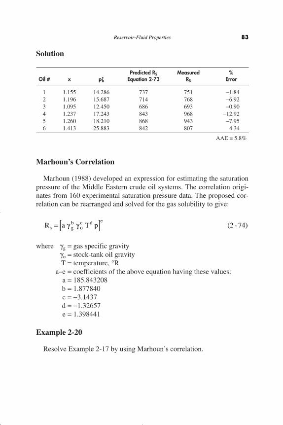
Solution
Predicted RS Measured %Oil # x p*b Equation 2-73 RS Error
1 1.155 14.286 737 751 -1.842 1.196 15.687 714 768 -6.923 1.095 12.450 686 693 -0.904 1.237 17.243 843 968 -12.925 1.260 18.210 868 943 -7.956 1.413 25.883 842 807 4.34
AAE = 5.8%
Marhoun’s Correlation
Marhoun (1988) developed an expression for estimating the saturationpressure of the Middle Eastern crude oil systems. The correlation origi-nates from 160 experimental saturation pressure data. The proposed cor-relation can be rearranged and solved for the gas solubility to give:
where gg = gas specific gravitygo = stock-tank oil gravityT = temperature, °R
a–e = coefficients of the above equation having these values:a = 185.843208b = 1.877840c = -3.1437d = -1.32657e = 1.398441
Example 2-20
Resolve Example 2-17 by using Marhoun’s correlation.
R a T ps gb
oc d e
= [ ]g g (2 - 74)
Reservoir-Fluid Properties 83
Reservoir Eng Hndbk Ch 02b 2001-10-24 09:26 Page 83

Solution
Predicted RS Measured %Oil # Equation 2-74 RS Error
1 740 751 -1.432 792 768 3.093 729 693 5.214 1041 968 7.555 845 943 -10.376 1186 807 47.03
AAE = 12.4%
The Petrosky-Farshad Correlation
Petrosky and Farshad (1993) used a nonlinear multiple regression soft-ware to develop a gas solubility correlation. The authors constructed aPVT database from 81 laboratory analyses from the Gulf of Mexico crudeoil system. Petrosky and Farshad proposed the following expression:
with
x = 7.916 (10-4) (API)1.5410 - 4.561(10-5 ) (T - 460)1.3911
where p = pressure, psiaT = temperature, °R
Example 2-21
Test the predictive capability of the Petrosky and Farshad equation byresolving Example 2-17.
Rp
s gx= +Ê
ˈ¯
ÈÎÍ
˘˚112 727
12 340 100 84391 73184
.. .
.
g (2 - 75)
84 Reservoir Engineering Handbook
Reservoir Eng Hndbk Ch 02b 2001-10-24 09:26 Page 84

Solution
Predicted RS Measured %Oil # x Equation 2-75 RS Error
1 0.2008 772 751 2.862 0.1566 726 768 -5.463 0.2101 758 693 9.324 0.1579 875 968 -9.575 0.1900 865 943 -8.286 0.0667 900 807 11.57
AAE = 7.84%
The gas solubility can also be calculated rigorously from the experi-mental measured PVT data at the specified pressure and temperature.The following expression relates the gas solubility Rs to oil density, spe-cific gravity of the oil, gas gravity, and the oil formation volume factor:
where ro = oil density, lb/ft3
Bo = oil formation volume factor, bbl/STBgo = specific gravity of the stock-tank oilgg = specific gravity of the solution gas
McCain (1991) pointed out that the weight average of separator andstock-tank gas specific gravities should be used for gg. The error in calcu-lating Rs by using the above equation will depend only on the accuracyof the available PVT data.
Example 2-22
Using the data of Example 2-17, estimate Rs by applying Equation 2-76.
RB
so o o
g= -r g
g62 4
0 0136.
.(2 - 76)
Reservoir-Fluid Properties 85
Reservoir Eng Hndbk Ch 02b 2001-10-24 09:26 Page 85
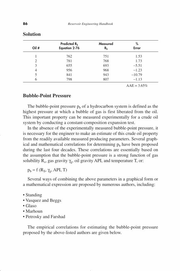
Solution
Predicted RS Measured %Oil # Equation 2-76 RS Error
1 762 751 1.532 781 768 1.733 655 693 -5.514 956 968 -1.235 841 943 -10.796 798 807 -1.13
AAE = 3.65%
Bubble-Point Pressure
The bubble-point pressure pb of a hydrocarbon system is defined as thehighest pressure at which a bubble of gas is first liberated from the oil.This important property can be measured experimentally for a crude oilsystem by conducting a constant-composition expansion test.
In the absence of the experimentally measured bubble-point pressure, itis necessary for the engineer to make an estimate of this crude oil propertyfrom the readily available measured producing parameters. Several graph-ical and mathematical correlations for determining pb have been proposedduring the last four decades. These correlations are essentially based onthe assumption that the bubble-point pressure is a strong function of gassolubility Rs, gas gravity gg, oil gravity API, and temperature T, or:
pb = f (RS, gg, API, T)
Several ways of combining the above parameters in a graphical form ora mathematical expression are proposed by numerous authors, including:
• Standing• Vasquez and Beggs• Glaso• Marhoun• Petrosky and Farshad
The empirical correlations for estimating the bubble-point pressureproposed by the above-listed authors are given below.
86 Reservoir Engineering Handbook
Reservoir Eng Hndbk Ch 02b 2001-10-24 09:26 Page 86
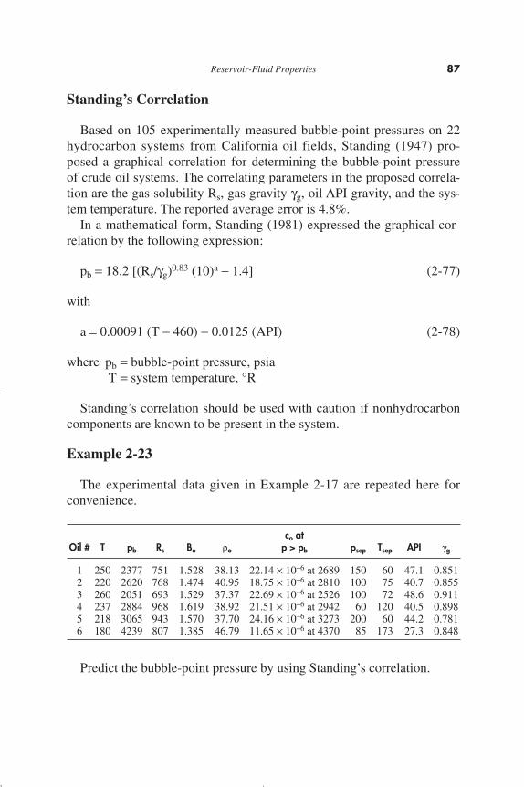
Standing’s Correlation
Based on 105 experimentally measured bubble-point pressures on 22hydrocarbon systems from California oil fields, Standing (1947) pro-posed a graphical correlation for determining the bubble-point pressureof crude oil systems. The correlating parameters in the proposed correla-tion are the gas solubility Rs, gas gravity gg, oil API gravity, and the sys-tem temperature. The reported average error is 4.8%.
In a mathematical form, Standing (1981) expressed the graphical cor-relation by the following expression:
pb = 18.2 [(Rs/gg)0.83 (10)a - 1.4] (2-77)
with
a = 0.00091 (T - 460) - 0.0125 (API) (2-78)
where pb = bubble-point pressure, psiaT = system temperature, °R
Standing’s correlation should be used with caution if nonhydrocarboncomponents are known to be present in the system.
Example 2-23
The experimental data given in Example 2-17 are repeated here forconvenience.
co atOil # T pb Rs Bo ro p > pb psep Tsep API gg
1 250 2377 751 1.528 38.13 22.14 ¥ 10-6 at 2689 150 60 47.1 0.8512 220 2620 768 1.474 40.95 18.75 ¥ 10-6 at 2810 100 75 40.7 0.8553 260 2051 693 1.529 37.37 22.69 ¥ 10-6 at 2526 100 72 48.6 0.9114 237 2884 968 1.619 38.92 21.51 ¥ 10-6 at 2942 60 120 40.5 0.8985 218 3065 943 1.570 37.70 24.16 ¥ 10-6 at 3273 200 60 44.2 0.7816 180 4239 807 1.385 46.79 11.65 ¥ 10-6 at 4370 85 173 27.3 0.848
Predict the bubble-point pressure by using Standing’s correlation.
Reservoir-Fluid Properties 87
Reservoir Eng Hndbk Ch 02b 2001-10-24 09:26 Page 87

Solution
Coeff. a Predicted pb Measured %Oil # Equation 2-78 Equation 2-77 pb Error
1 -0.3613 2181 2392 -8.82 -0.3086 2503 2635 -5.03 -0.3709 1883 2066 -8.84 -0.3115 2896 2899 -0.15 -0.3541 2884 3060 -5.76 -0.1775 3561 4254 -16.3
AAE = 7.4%
McCain (1991) suggested that by replacing the specific gravity of thegas in Equation 2-77 with that of the separator gas, i.e., excluding the gasfrom the stock tank would improve the accuracy of the equation.
Example 2-24
Using the data of Example 2-23 and given the following separator gasgravities, estimate the bubble-point pressure by applying Standing’s cor-relation.
Oil # Separator Gas Gravity
1 0.7552 0.7863 0.8014 0.8885 0.7056 0.813
Solution
Oil # Predicted pb Measured pb % Error
1 2411 2392 0.832 2686 2635 1.933 2098 2066 1.534 2923 2899 0.845 3143 3060 2.706 3689 4254 -13.27
AAE = 3.5%
88 Reservoir Engineering Handbook
Reservoir Eng Hndbk Ch 02b 2001-10-24 09:26 Page 88

The Vasquez-Beggs Correlation
Vasquez and Beggs’ gas solubility correlation as presented by Equa-tion 2-71 can be solved for the bubble-point pressure pb to give:
with
a = - C3 API/T
The gas specific gravity ggs at the reference separator pressure isdefined by Equation 2-72. The coefficients C1, C2, and C3 have the fol-lowing values:
Coefficient API ≤ 30 API > 30
C1 27.624 56.18C2 0.914328 0.84246C3 11.172 10.393
Example 2-25
Rework Example 2-23 by applying Equation 2-79.
Solution
ggs Predicted Measured %Oil # Equation 2-72 a pb pb Error
1 0.873 -0.689 2319 2392 -3.072 0.855 -0.622 2741 2635 4.033 0.911 -0.702 2043 2066 -1.144 0.850 -0.625 3331 2899 14.915 0.814 -0.678 3049 3060 -0.366 0.834 -0.477 4093 4254 -3.78
AAE= 4.5%
p C Rb s gsa C
= [ ]( / ) ( )1210g (2 - 79)
Reservoir-Fluid Properties 89
Reservoir Eng Hndbk Ch 02b 2001-10-24 09:26 Page 89
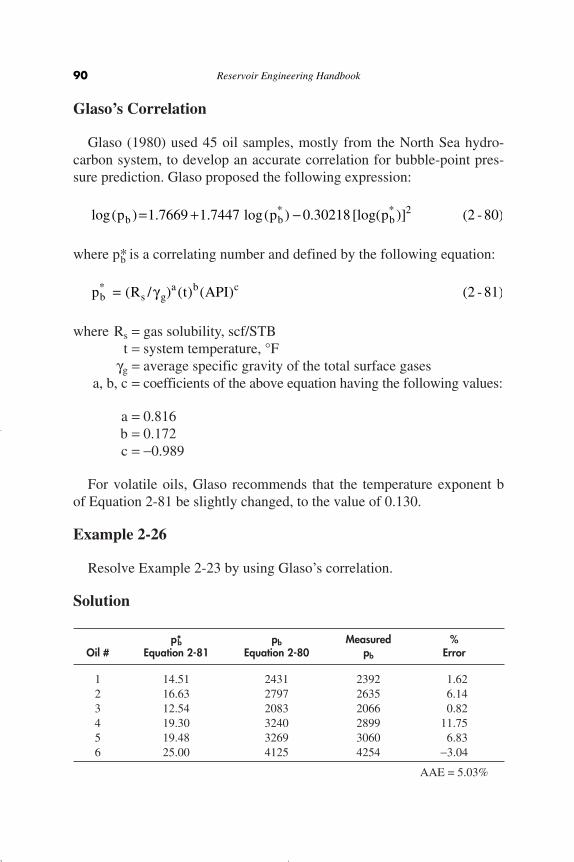
Glaso’s Correlation
Glaso (1980) used 45 oil samples, mostly from the North Sea hydro-carbon system, to develop an accurate correlation for bubble-point pres-sure prediction. Glaso proposed the following expression:
where p*b is a correlating number and defined by the following equation:
where Rs = gas solubility, scf/STBt = system temperature, °F
gg = average specific gravity of the total surface gasesa, b, c = coefficients of the above equation having the following values:
a = 0.816b = 0.172c = -0.989
For volatile oils, Glaso recommends that the temperature exponent bof Equation 2-81 be slightly changed, to the value of 0.130.
Example 2-26
Resolve Example 2-23 by using Glaso’s correlation.
Solution
p*b pb Measured %Oil # Equation 2-81 Equation 2-80 pb Error
1 14.51 2431 2392 1.622 16.63 2797 2635 6.143 12.54 2083 2066 0.824 19.30 3240 2899 11.755 19.48 3269 3060 6.836 25.00 4125 4254 -3.04
AAE = 5.03%
p R t APIb s ga b c* ( / ) ( ) ( )= g (2 - 81)
log( ) . . log( ) . [log( )]* *p p pb b b= + -1 7669 1 7447 0 30218 2 (2 - 80)
90 Reservoir Engineering Handbook
Reservoir Eng Hndbk Ch 02b 2001-10-24 09:26 Page 90
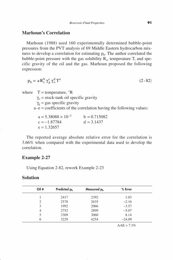
Marhoun’s Correlation
Marhoun (1988) used 160 experimentally determined bubble-pointpressures from the PVT analysis of 69 Middle Eastern hydrocarbon mix-tures to develop a correlation for estimating pb. The author correlated thebubble-point pressure with the gas solubility Rs, temperature T, and spe-cific gravity of the oil and the gas. Marhoun proposed the followingexpression:
where T = temperature, °Rgo = stock-tank oil specific gravitygg = gas specific gravity
a–e = coefficients of the correlation having the following values:
a = 5.38088 ¥ 10-3 b = 0.715082c = -1.87784 d = 3.1437e = 1.32657
The reported average absolute relative error for the correlation is3.66% when compared with the experimental data used to develop thecorrelation.
Example 2-27
Using Equation 2-82, rework Example 2-23
Solution
Oil # Predicted pb Measured pb % Error
1 2417 2392 1.032 2578 2635 -2.163 1992 2066 -3.574 2752 2899 -5.075 3309 3060 8.146 3229 4254 -24.09
AAE = 7.3%
p a R Tb sb
gc
od e= g g (2 - 82)
Reservoir-Fluid Properties 91
Reservoir Eng Hndbk Ch 02b 2001-10-24 09:26 Page 91
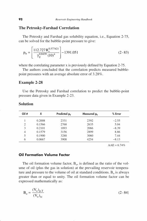
The Petrosky-Farshad Correlation
The Petrosky and Farshad gas solubility equation, i.e., Equation 2-75,can be solved for the bubble-point pressure to give:
where the correlating parameter x is previously defined by Equation 2-75.The authors concluded that the correlation predicts measured bubble-
point pressures with an average absolute error of 3.28%.
Example 2-28
Use the Petrosky and Farshad correlation to predict the bubble-pointpressure data given in Example 2-23.
Solution
Oil # X Predicted pb Measured pb % Error
1 0.2008 2331 2392 -2.552 0.1566 2768 2635 5.043 0.2101 1893 2066 -8.394 0.1579 3156 2899 8.865 0.1900 3288 3060 7.446 0.0667 3908 4254 -8.13
AAE = 6.74%
Oil Formation Volume Factor
The oil formation volume factor, Bo, is defined as the ratio of the vol-ume of oil (plus the gas in solution) at the prevailing reservoir tempera-ture and pressure to the volume of oil at standard conditions. Bo is alwaysgreater than or equal to unity. The oil formation volume factor can beexpressed mathematically as:
BV
Voo p T
o sc=
( )
( ), (2 - 84)
pR
bs
gx=
È
ÎÍÍ
˘
˚˙˙
-112 727
101391 051
0 577421
0 8439.
( ).
.
.g(2 - 83)
92 Reservoir Engineering Handbook
Reservoir Eng Hndbk Ch 02b 2001-10-24 09:26 Page 92

where Bo = oil formation volume factor, bbl/STB(Vo)p,T = volume of oil under reservoir pressure p and temperature T,
bbl(Vo)sc = volume of oil is measured under standard conditions, STB
A typical oil formation factor curve, as a function of pressure for anundersaturated crude oil (pi > pb), is shown in Figure 2-8. As the pressureis reduced below the initial reservoir pressure pi, the oil volume increasesdue to the oil expansion. This behavior results in an increase in the oil for-mation volume factor and will continue until the bubble-point pressure isreached. At pb, the oil reaches its maximum expansion and consequentlyattains a maximum value of Bob for the oil formation volume factor. As thepressure is reduced below pb, volume of the oil and Bo are decreased as thesolution gas is liberated. When the pressure is reduced to atmosphericpressure and the temperature to 60°F, the value of Bo is equal to one.
Most of the published empirical Bo correlations utilize the followinggeneralized relationship:
B f R To s g o= ( , , , )g g
Reservoir-Fluid Properties 93
Figure 2-8. Oil formation volume factor versus pressure.
Reservoir Eng Hndbk Ch 02b 2001-10-24 09:26 Page 93

Six different methods of predicting the oil formation volume factor arepresented below:
• Standing’s correlation• The Vasquez-Beggs correlation• Glaso’s correlation• Marhoun’s correlation• The Petrosky-Farshad correlation• Other correlations
It should be noted that all the correlations could be used for any pres-sure equal to or below the bubble-point pressure.
Standing’s Correlation
Standing (1947) presented a graphical correlation for estimating the oilformation volume factor with the gas solubility, gas gravity, oil gravity,and reservoir temperature as the correlating parameters. This graphicalcorrelation originated from examining a total of 105 experimental datapoints on 22 different California hydrocarbon systems. An average errorof 1.2% was reported for the correlation.
Standing (1981) showed that the oil formation volume factor can beexpressed more conveniently in a mathematical form by the followingequation:
where T = temperature, °Rgo = specific gravity of the stock-tank oilgg = specific gravity of the solution gas
The Vasquez-Beggs Correlation
Vasquez and Beggs (1980) developed a relationship for determiningBo as a function of Rs, go, gg, and T. The proposed correlation was basedon 6,000 measurements of Bo at various pressures. Using the regression
bggo s
g
oR T= +
ÊËÁ
ˆ¯
+ -È
ÎÍÍ
˘
˚˙˙
0 9759 0 000120 1 25 4600 5 1 2
. . . ( ). .
(2 - 85)
94 Reservoir Engineering Handbook
Reservoir Eng Hndbk Ch 02b 2001-10-24 09:26 Page 94

analysis technique, Vasquez and Beggs found the following equation tobe the best form to reproduce the measured data:
where R = gas solubility, scf/STBT = temperature, °R
ggs = gas specific gravity as defined by Equation 2-72
Values for the coefficients C1, C2 and C3 are given below:
Coefficient API ≤ 30 API > 30
C1 4.677 ¥ 10-4 4.670 ¥ 10-4
C2 1.751 ¥ 10-5 1.100 ¥ 10-5
C3 -1.811 ¥ 10-8 1.337 ¥ 10-9
Vasquez and Beggs reported an average error of 4.7% for the proposedcorrelation.
Glaso’s Correlation
Glaso (1980) proposed the following expressions for calculating theoil formation volume factor:
Bo = 1.0 + 10A (2-87)
where
A = -6.58511 + 2.91329 log B*ob - 0.27683 (log B*ob)2 (2-88)
B*ob is a correlating number and is defined by the following equation:
where T = temperature, °Rgo = specific gravity of the stock-tank oil
B R Tob sg
o
*.
. ( )=ÊËÁ
ˆ¯
+ -gg
0 526
0 968 460 (2 - 89)
B C R TAPI
C C Ro sgs
s= + + -Ê
ËÁ
ˆ
¯˜ +1 0 5201 2 3. ( ) [ ]
g(2 - 86)
Reservoir-Fluid Properties 95
Reservoir Eng Hndbk Ch 02b 2001-10-24 09:26 Page 95

The above correlations were originated from studying PVT data on 45oil samples. The average error of the correlation was reported at -0.43%with a standard deviation of 2.18%.
Sutton and Farshad (1984) concluded that Glaso’s correlation offersthe best accuracy when compared with the Standing and Vasquez-Beggscorrelations. In general, Glaso’s correlation underpredicts formation vol-ume factor. Standing’s expression tends to overpredict oil formation vol-ume factors greater than 1.2 bbl/STB. The Vasquez-Beggs correlationtypically overpredicts the oil formation volume factor.
Marhoun’s Correlation
Marhoun (1988) developed a correlation for determining the oil for-mation volume factor as a function of the gas solubility, stock-tank oilgravity, gas gravity, and temperature. The empirical equation was devel-oped by use of the nonlinear multiple regression analysis on 160 experi-mental data points. The experimental data were obtained from 69 MiddleEastern oil reserves. The author proposed the following expression:
Bo = 0.497069 + 0.862963 ¥ 10-3 T + 0.182594 ¥ 10-2 F+ 0.318099 ¥ 10-5 F2 (2-90)
with the correlating parameter F as defined by the following equation:
F = Rsa gg
b goc (2-91)
The coefficients a, b and c have the following values:
a = 0.742390b = 0.323294c = -1.202040
where T is the system temperature in °R.
The Petrosky-Farshad Correlation
Petrosky and Farshad (1993) proposed a new expression for estimatingBo. The proposed relationship is similar to the equation developed byStanding; however, the equation introduces three additional fitting para-meters in order to increase the accuracy of the correlation.
96 Reservoir Engineering Handbook
Reservoir Eng Hndbk Ch 02b 2001-10-24 09:26 Page 96
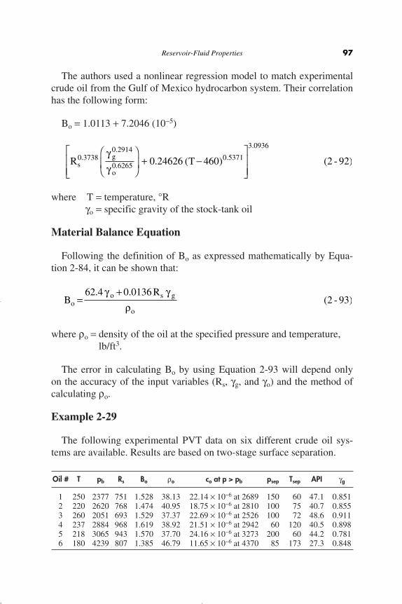
The authors used a nonlinear regression model to match experimentalcrude oil from the Gulf of Mexico hydrocarbon system. Their correlationhas the following form:
Bo = 1.0113 + 7.2046 (10-5)
where T = temperature, °Rgo = specific gravity of the stock-tank oil
Material Balance Equation
Following the definition of Bo as expressed mathematically by Equa-tion 2-84, it can be shown that:
where ro = density of the oil at the specified pressure and temperature,lb/ft3.
The error in calculating Bo by using Equation 2-93 will depend onlyon the accuracy of the input variables (Rs, gg, and go) and the method ofcalculating ro.
Example 2-29
The following experimental PVT data on six different crude oil sys-tems are available. Results are based on two-stage surface separation.
Oil # T pb Rs Bo ro co at p > pb psep Tsep API gg
1 250 2377 751 1.528 38.13 22.14 ¥ 10-6 at 2689 150 60 47.1 0.8512 220 2620 768 1.474 40.95 18.75 ¥ 10-6 at 2810 100 75 40.7 0.8553 260 2051 693 1.529 37.37 22.69 ¥ 10-6 at 2526 100 72 48.6 0.9114 237 2884 968 1.619 38.92 21.51 ¥ 10-6 at 2942 60 120 40.5 0.8985 218 3065 943 1.570 37.70 24.16 ¥ 10-6 at 3273 200 60 44.2 0.7816 180 4239 807 1.385 46.79 11.65 ¥ 10-6 at 4370 85 173 27.3 0.848
BR
oo s g
o=
+62 4 0 0136. .g gr
(2 - 93)
R Tsg
o
0 37380 2914
0 62650 5371
3 0936
0 24626 460..
..
.
. ( )gg
Ê
ËÁ
ˆ
¯˜ + -
È
ÎÍÍ
˘
˚˙˙
(2 - 92)
Reservoir-Fluid Properties 97
Reservoir Eng Hndbk Ch 02b 2001-10-24 09:26 Page 97
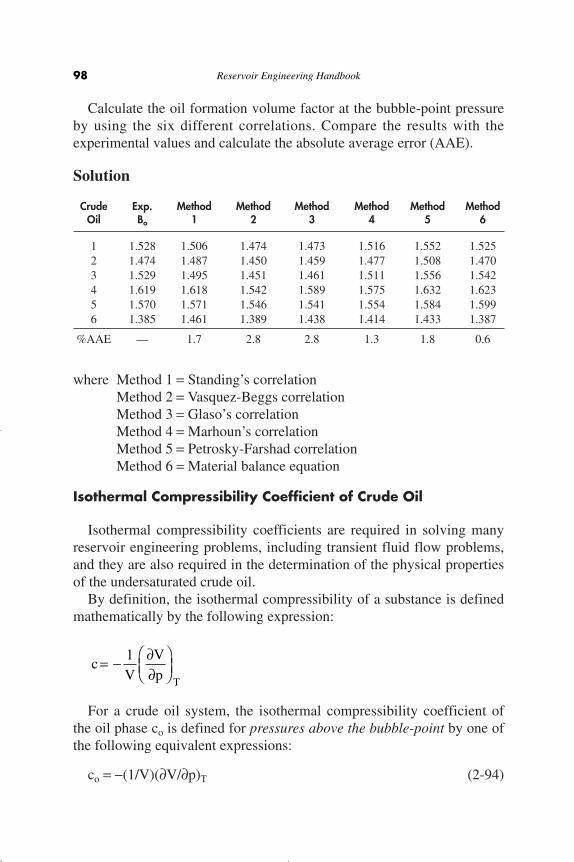
Calculate the oil formation volume factor at the bubble-point pressureby using the six different correlations. Compare the results with theexperimental values and calculate the absolute average error (AAE).
Solution
Crude Exp. Method Method Method Method Method MethodOil Bo 1 2 3 4 5 6
1 1.528 1.506 1.474 1.473 1.516 1.552 1.5252 1.474 1.487 1.450 1.459 1.477 1.508 1.4703 1.529 1.495 1.451 1.461 1.511 1.556 1.5424 1.619 1.618 1.542 1.589 1.575 1.632 1.6235 1.570 1.571 1.546 1.541 1.554 1.584 1.5996 1.385 1.461 1.389 1.438 1.414 1.433 1.387
%AAE — 1.7 2.8 2.8 1.3 1.8 0.6
where Method 1 = Standing’s correlationMethod 2 = Vasquez-Beggs correlationMethod 3 = Glaso’s correlationMethod 4 = Marhoun’s correlationMethod 5 = Petrosky-Farshad correlationMethod 6 = Material balance equation
Isothermal Compressibility Coefficient of Crude Oil
Isothermal compressibility coefficients are required in solving manyreservoir engineering problems, including transient fluid flow problems,and they are also required in the determination of the physical propertiesof the undersaturated crude oil.
By definition, the isothermal compressibility of a substance is definedmathematically by the following expression:
For a crude oil system, the isothermal compressibility coefficient ofthe oil phase co is defined for pressures above the bubble-point by one ofthe following equivalent expressions:
co = -(1/V)(∂V/∂p)T (2-94)
cV
Vp T
= - ∂∂
ÊËÁ
ˆ¯
1
98 Reservoir Engineering Handbook
Reservoir Eng Hndbk Ch 02b 2001-10-24 09:26 Page 98
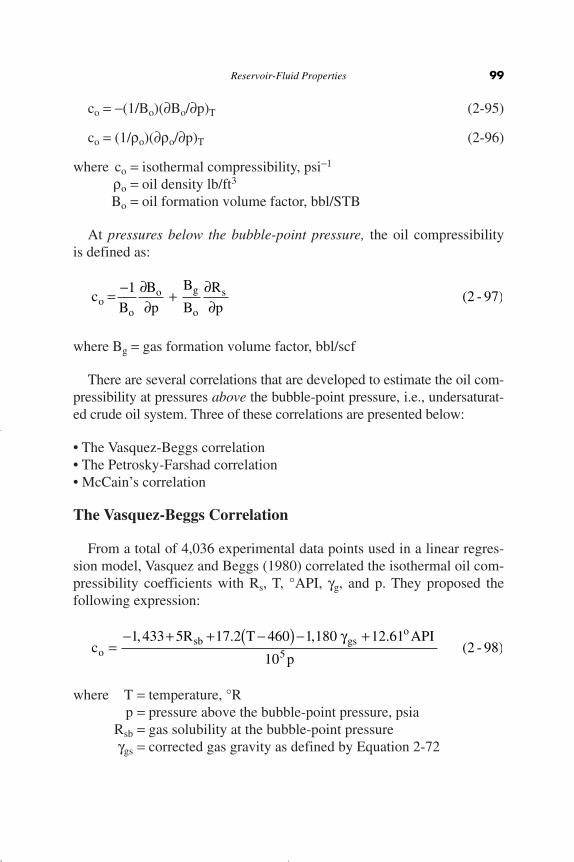
co = -(1/Bo)(∂Bo/∂p)T (2-95)
co = (1/ro)(∂ro/∂p)T (2-96)
where co = isothermal compressibility, psi-1
ro = oil density lb/ft3
Bo = oil formation volume factor, bbl/STB
At pressures below the bubble-point pressure, the oil compressibilityis defined as:
where Bg = gas formation volume factor, bbl/scf
There are several correlations that are developed to estimate the oil com-pressibility at pressures above the bubble-point pressure, i.e., undersaturat-ed crude oil system. Three of these correlations are presented below:
• The Vasquez-Beggs correlation• The Petrosky-Farshad correlation• McCain’s correlation
The Vasquez-Beggs Correlation
From a total of 4,036 experimental data points used in a linear regres-sion model, Vasquez and Beggs (1980) correlated the isothermal oil com-pressibility coefficients with Rs, T, °API, gg, and p. They proposed thefollowing expression:
where T = temperature, °Rp = pressure above the bubble-point pressure, psia
Rsb = gas solubility at the bubble-point pressureggs = corrected gas gravity as defined by Equation 2-72
cR T API
posb gs
o
=- + + -( ) - +1 433 5 17 2 460 1 180 12 61
105
, . , .g(2 - 98)
cB
Bp
B
BRpo
o
o g
o
s= - ∂∂
+ ∂∂
1(2 - 97)
Reservoir-Fluid Properties 99
Reservoir Eng Hndbk Ch 02b 2001-10-24 09:26 Page 99
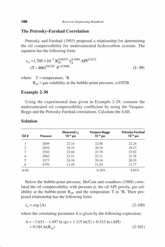
The Petrosky-Farshad Correlation
Petrosky and Farshad (1993) proposed a relationship for determiningthe oil compressibility for undersaturated hydrocarbon systems. Theequation has the following form:
where T = temperature, °RRsb = gas solubility at the bubble-point pressure, scf/STB
Example 2-30
Using the experimental data given in Example 2-29, estimate theundersaturated oil compressibility coefficient by using the Vasquez-Beggs and the Petrosky-Farshad correlations. Calculate the AAE.
Solution
Measured co Vasquez-Beggs Petrosky-FarshadOil # Pressure 10-6 psi 10-6 psi 10-6 psi
1 2689 22.14 22.88 22.242 2810 18.75 20.16 19.273 2526 22.60 23.78 22.924 2942 21.51 22.31 21.785 3273 24.16 20.16 20.396 4370 11.45 11.54 11.77
AAE 6.18% 4.05%
Below the bubble-point pressure, McCain and coauthors (1988) corre-lated the oil compressibility with pressure r, the oil API gravity, gas sol-ubility at the bubble-point Rsb, and the temperature T in °R. Their pro-posed relationship has the following form:
co = exp (A) (2-100)
where the correlating parameter A is given by the following expression:
A = -7.633 - 1.497 ln (p) + 1.115 ln(T) + 0.533 ln (API)+ 0.184 ln(Rsp) (2-101)
c R API
T Po sb g= ¥
-
-
-
1 705 10
460
7 0 69357 0 1885 0 3272
0 6729 0 5906
.
( )
. . .
. .
g(2 - 99)
100 Reservoir Engineering Handbook
Reservoir Eng Hndbk Ch 02b 2001-10-24 09:26 Page 100

The authors suggested that the accuracy of the Equation 2-100 can besubstantially improved if the bubble-point pressure is known. Theyimproved correlating parameter A by including the bubble-point pressurepb as one of the parameters in the above equation, to give:
A = -7.573 - 1.45 ln (p) - 0.383 ln (Pb) + 1.402 ln (T)+ 0.256 ln (API) + 0.449 ln (Rsb) (2-102)
Analytically, Standing’s correlations for Rs (Equation 2-70) and bo
(Equation 2-85) can be differentiated with respect to the pressure p to give:
The above two expressions can be substituted into Equation 2-97 togive the following relationship:
where p = pressure, psiaT = temperature, °R
Bg = gas formation volume factor at pressure p, bbl/scfRs = gas solubility at pressure p, scf/STBBo = oil formation volume factor at p, bbl/STB
go = specific gravity of the stock-tank oilgg = specific gravity of the solution gas
cR
B p
R T B
os
o
g
os
g
og
= -+
¥ + -È
ÎÍÍ
˘
˚˙˙
-ÏÌÔ
ÓÔ
¸˝Ô
Ô
( . . )
. . ( )
.
0 83 21 75
0 00014 1 25 460
0 12gg
gg
(2 -105)
∂∂
=+
È
ÎÍ
˘
˚˙
ÊËÁ
ˆ¯
¥ÊËÁ
ˆ¯
+ -( )È
ÎÍÍ
˘
˚˙˙
Bp
Rp
R T
o s g
o
sg
o
0 0001440 83 21 75
1 25 460
0 5
0 5 0 12
.. .
.
.
. .
gg
gg
(2 -104)
∂∂
=+
R
p
R
0.83 p 21.75(2 - 103)s s
Reservoir-Fluid Properties 101
Reservoir Eng Hndbk Ch 02b 2001-10-24 09:26 Page 101
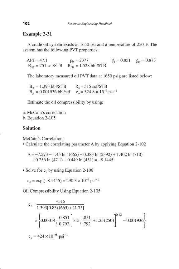
Example 2-31
A crude oil system exists at 1650 psi and a temperature of 250°F. Thesystem has the following PVT properties:
API = 47.1 pb = 2377 gg = 0.851 ggs = 0.873Rsb = 751 scf/STB Bob = 1.528 bbl/STB
The laboratory measured oil PVT data at 1650 psig are listed below:
Bo = 1.393 bbl/STB Rs = 515 scf/STBBg = 0.001936 bbl/scf co = 324.8 ¥ 15-6 psi-1
Estimate the oil compressibility by using:
a. McCain’s correlationb. Equation 2-105
Solution
McCain’s Correlation:• Calculate the correlating parameter A by applying Equation 2-102
A = -7.573 - 1.45 ln (1665) - 0.383 ln (2392) + 1.402 ln (710)+ 0.256 ln (47.1) + 0.449 ln (451) = -8.1445
• Solve for co by using Equation 2-100
co = exp (-8.1445) = 290.3 ¥ 10-6 psi-1
Oil Compressibility Using Equation 2-105
c
c psi
o
o
= -+
¥ +È
ÎÍ
˘
˚˙ -
ÏÌÔ
ÓÔ
¸˝Ô
Ô
= ¥ - -
5151 393 0 83 1665 21 75
0 000140 8510 792
515851792
1 25 250 0 001936
424 10
0 12
6 1
. [ . ( ) . ]
...
.
.. ( ) .
.
102 Reservoir Engineering Handbook
Reservoir Eng Hndbk Ch 02b 2001-10-24 09:26 Page 102

It should be pointed out that when it is necessary to establish PVTrelationships for the hydrocarbon system through correlations or byextrapolation, care should be exercised to see that the PVT functions areconsistent.
This consistency is assured if the increase in oil volume with increas-ing pressure is less than the decrease in volume associated with the gasgoing into solution. Since the oil compressibility coefficient co asexpressed by Equation 2-97 must be positive, that leads to the followingconsistency criteria:
This consistency can easily be checked in the tabular form of PVTdata. The PVT consistency errors most frequently occur at higher pres-sures where the gas formation volume factor, Bg, assumes relativelysmall values.
Oil Formation Volume Factor for Undersaturated Oils
With increasing pressures above the bubble-point pressure, the oil for-mation volume factor decreases due to the compression of the oil, asillustrated schematically in Figure 2-9.
To account for the effects of oil compression on Bo, the oil formationvolume factor at the bubble-point pressure is first calculated by using anyof the methods previously described. The calculated Bo is then adjustedto account for the effect if increasing the pressure above the bubble-pointpressure. This adjustment step is accomplished by using the isothermalcompressibility coefficient as described below.
The isothermal compressibility coefficient (as expressed mathemati-cally by Equation 2-94) can be equivalently written in terms of the oilformation volume factor:
The above relationship can be rearranged and integrated to produce
- =Ú Úpb
p
ooBob
Booc dp
BdB
1(2 -107)
cB
Bpo
o
o= - ∂∂
1
∂∂
< ∂∂
Bp
BRp
og
s (2 -106)
Reservoir-Fluid Properties 103
Reservoir Eng Hndbk Ch 02b 2001-10-24 09:26 Page 103

Evaluating co at the arithmetic average pressure and concluding theintegration procedure to give:
Bo = Bob exp [-co (p - pb)] (2-108)
where Bo = oil formation volume factor at the pressure of interest,bbl/STB
Bob = oil formation volume factor at the bubble-point pressure,bbl/STB
p = pressure of interest, psiapb = bubble-point pressure, psia
Replacing with the Vasquez-Beggs’ co expression, i.e., Equation 2-98,and integrating the resulting equation gives:
B B Ap
po obb
= -ÊËÁ
ˆ¯
È
ÎÍÍ
˘
˚˙˙
exp ln (2 -109)
104 Reservoir Engineering Handbook
Figure 2-9. Volume versus pressure relationship.
Reservoir Eng Hndbk Ch 02b 2001-10-24 09:26 Page 104

where
A = 10-5 [-1,433 + 5 Rsb + 17.2(T - 460) - 1,180 ggs + 12.61 API]
Replacing co in Equation 2-107 with the Petrosky-Farshad expression(i.e., Equation 2-99) and integrating gives:
with the correlating parameter A as defined by:
where T = temperature, °Rp = pressure, psia
Rsb = gas solubility at the bubble-point pressure
Example 2-32
Using the PVT data given in Example 2-31, calculate the oil formationvolume factor at 5000 psig by using:
a. Equation 2-109b. Equation 2-110
The experimental measured Bo is 1.457 bbl/STB.
Solution
Using Equation 2-109:
• Calculate the parameter A:
A = 10-5 [-1433 + 5 (751) + 17.2 (250) - 1180 (0.873)+ 12.61 (47.1)] = 0.061858
• Apply Equation 2-109:
B bbl STBo = - ÊË
ˆ¯
ÈÎÍ
˘˚
=1 528 0 06185850152392
1 459. exp . ln . /
A R API Tsb g= --4 1646 10 4607 0 69357 0 1885 0 3272 0 6729. ( ) ( ) ( ). . . .g (2 -111)
B B exp [ A (p p )] (2 - 110)o ob
0.4094
b
0.4094= - -
Reservoir-Fluid Properties 105
Reservoir Eng Hndbk Ch 02b 2001-10-24 09:26 Page 105
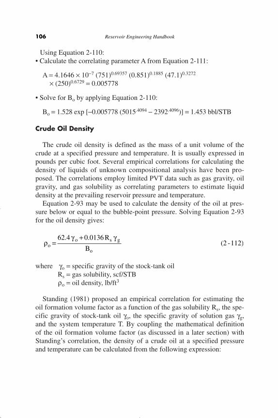
Using Equation 2-110:• Calculate the correlating parameter A from Equation 2-111:
A = 4.1646 ¥ 10-7 (751)0.69357 (0.851)0.1885 (47.1)0.3272
¥ (250)0.6729 = 0.005778
• Solve for Bo by applying Equation 2-110:
Bo = 1.528 exp [-0.005778 (5015.4094 - 2392.4096)] = 1.453 bbl/STB
Crude Oil Density
The crude oil density is defined as the mass of a unit volume of thecrude at a specified pressure and temperature. It is usually expressed inpounds per cubic foot. Several empirical correlations for calculating thedensity of liquids of unknown compositional analysis have been pro-posed. The correlations employ limited PVT data such as gas gravity, oilgravity, and gas solubility as correlating parameters to estimate liquiddensity at the prevailing reservoir pressure and temperature.
Equation 2-93 may be used to calculate the density of the oil at pres-sure below or equal to the bubble-point pressure. Solving Equation 2-93for the oil density gives:
where go = specific gravity of the stock-tank oilRs = gas solubility, scf/STBro = oil density, lb/ft3
Standing (1981) proposed an empirical correlation for estimating theoil formation volume factor as a function of the gas solubility Rs, the spe-cific gravity of stock-tank oil go, the specific gravity of solution gas gg,and the system temperature T. By coupling the mathematical definitionof the oil formation volume factor (as discussed in a later section) withStanding’s correlation, the density of a crude oil at a specified pressureand temperature can be calculated from the following expression:
rg g
oo s g
o
R
B=
+62 4 0 0136. .(2 -112)
106 Reservoir Engineering Handbook
Reservoir Eng Hndbk Ch 02b 2001-10-24 09:26 Page 106

where T = system temperature, °Rgo = specific gravity of the stock-tank oil
Example 2-33
Using the experimental PVT data given in Example 2-29 for the sixdifferent crude oil systems, calculate the oil density by using Equations2-112 and 2-113. Compare the results with the experimental values andcalculate the absolute average error (AAE).
Solution
Measured OilCrude Oil Density Equation 2-112 Equation 2-113
1 38.13 38.04 38.312 40.95 40.85 40.183 37.37 37.68 38.264 42.25 41.52 40.395 37.70 38.39 38.086 46.79 46.86 44.11
AAE 0.84% 2.65%
Density of the oil at pressures above the bubble-point pressure can becalculated with:
ro = rob exp [co (p - pb)] (2-114)
where ro = density of the oil at pressure p, lb/ft3
rob = density of the oil at the bubble-point pressure, lb/ft3
co = isothermal compressibility coefficient at average pressure, psi-1
rg g
gg
oo s g
sg
o
R
R T
=+
+ÊËÁ
ˆ¯
+ -( )È
ÎÍÍ
˘
˚˙˙
62 4 0 0136
0 972 0 000147 1 25 4605 1 175
. .
. . .. . (2 -113)
Reservoir-Fluid Properties 107
Reservoir Eng Hndbk Ch 02b 2001-10-24 09:26 Page 107
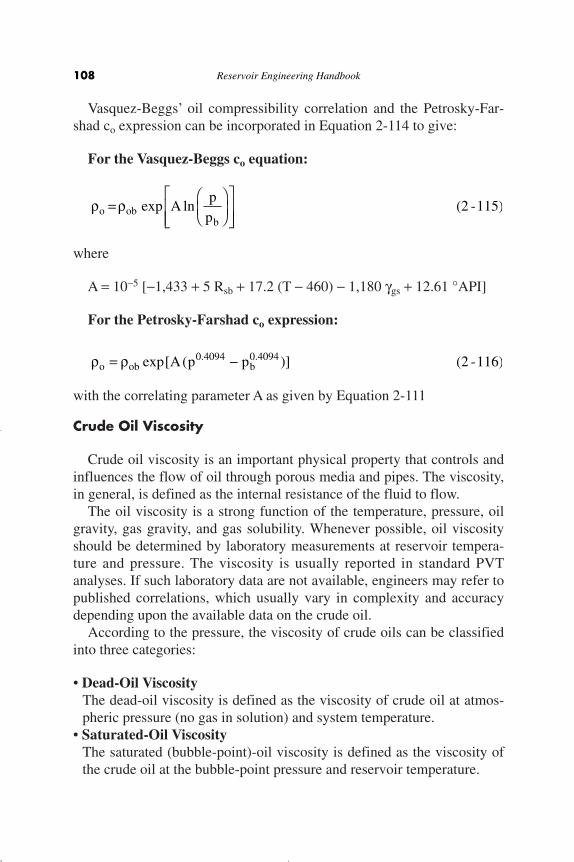
Vasquez-Beggs’ oil compressibility correlation and the Petrosky-Far-shad co expression can be incorporated in Equation 2-114 to give:
For the Vasquez-Beggs co equation:
where
A = 10-5 [-1,433 + 5 Rsb + 17.2 (T - 460) - 1,180 ggs + 12.61 °API]
For the Petrosky-Farshad co expression:
with the correlating parameter A as given by Equation 2-111
Crude Oil Viscosity
Crude oil viscosity is an important physical property that controls andinfluences the flow of oil through porous media and pipes. The viscosity,in general, is defined as the internal resistance of the fluid to flow.
The oil viscosity is a strong function of the temperature, pressure, oilgravity, gas gravity, and gas solubility. Whenever possible, oil viscosityshould be determined by laboratory measurements at reservoir tempera-ture and pressure. The viscosity is usually reported in standard PVTanalyses. If such laboratory data are not available, engineers may refer topublished correlations, which usually vary in complexity and accuracydepending upon the available data on the crude oil.
According to the pressure, the viscosity of crude oils can be classifiedinto three categories:
• Dead-Oil ViscosityThe dead-oil viscosity is defined as the viscosity of crude oil at atmos-pheric pressure (no gas in solution) and system temperature.
• Saturated-Oil ViscosityThe saturated (bubble-point)-oil viscosity is defined as the viscosity ofthe crude oil at the bubble-point pressure and reservoir temperature.
r ro ob bA p p= -exp[ ( )]. .0 4094 0 4094 (2 -116)
r ro obb
Ap
p=
ÊËÁ
ˆ¯
È
ÎÍÍ
˘
˚˙˙
exp ln (2 -115)
108 Reservoir Engineering Handbook
Reservoir Eng Hndbk Ch 02b 2001-10-24 09:26 Page 108

• Undersaturated-Oil ViscosityThe undersaturated-oil viscosity is defined as the viscosity of the crudeoil at a pressure above the bubble-point and reservoir temperature.
Estimation of the oil viscosity at pressures equal to or below the bub-ble-point pressure is a two-step procedure:
Step 1. Calculate the viscosity of the oil without dissolved gas (dead oil),mob, at the reservoir temperature.
Step 2. Adjust the dead-oil viscosity to account for the effect of the gassolubility at the pressure of interest.
At pressures greater than the bubble-point pressure of the crude oil,another adjustment step, i.e. Step 3, should be made to the bubble-pointoil viscosity, mob, to account for the compression and the degree of under-saturation in the reservoir. A brief description of several correlations thatare widely used in estimating the oil viscosity in the above three steps isgiven below.
METHODS OF CALCULATING VISCOSITYOF THE DEAD OIL
Several empirical methods are proposed to estimate the viscosity ofthe dead oil, including:
• Beal’s correlation• The Beggs-Robinson correlation• Glaso’s correlation
These three methods are presented below.
Beal’s Correlation
From a total of 753 values for dead-oil viscosity at and above 100°F,Beal (1946) developed a graphical correlation for determining the viscos-ity of the dead oil as a function of temperature and the API gravity of thecrude. Standing (1981) expressed the proposed graphical correlation in amathematical relationship as follows:
Reservoir-Fluid Properties 109
Reservoir Eng Hndbk Ch 02b 2001-10-24 09:26 Page 109

with
a = 10(0.43 + 8.33/API)
where mod = viscosity of the dead oil as measured at 14.7 psia andreservoir temperature, cp
T = temperature, °R
The Beggs-Robinson Correlation
Beggs and Robinson (1975) developed an empirical correlation fordetermining the viscosity of the dead oil. The correlation originated fromanalyzing 460 dead-oil viscosity measurements. The proposed relation-ship is expressed mathematically as follows:
mod = 10x - 1 (2-118)
where x = Y (T - 460)-1.163
Y = 10Z
Z = 3.0324 - 0.02023°API
An average error of -0.64% with a standard deviation of 13.53% wasreported for the correlation when tested against the data used for itsdevelopment. Sutton and Farshad (1980) reported an error of 114.3%when the correlation was tested against 93 cases from the literature.
Glaso’s Correlation
Glaso (1980) proposed a generalized mathematical relationship forcomputing the dead-oil viscosity. The relationship was developed fromexperimental measurements on 26 crude oil samples. The correlation hasthe following form:
where the coefficient a is given by:
a = 10.313 [log(T - 460)] -36.447
modaT API= - -[ . ( )] ( ) [log ( )].3 141 10 46010 3 444 (2 -119)
m od
7
4.53
a
0.321.8(10 )
API
360
T 260(2 - 117)= +
-
Ê
ËÁˆ
¯
ÊËÁ
ˆ¯
110 Reservoir Engineering Handbook
Reservoir Eng Hndbk Ch 02b 2001-10-24 09:26 Page 110
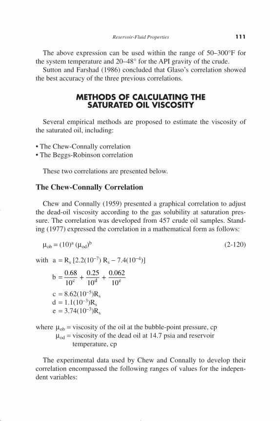
The above expression can be used within the range of 50–300°F forthe system temperature and 20–48° for the API gravity of the crude.
Sutton and Farshad (1986) concluded that Glaso’s correlation showedthe best accuracy of the three previous correlations.
METHODS OF CALCULATING THESATURATED OIL VISCOSITY
Several empirical methods are proposed to estimate the viscosity ofthe saturated oil, including:
• The Chew-Connally correlation• The Beggs-Robinson correlation
These two correlations are presented below.
The Chew-Connally Correlation
Chew and Connally (1959) presented a graphical correlation to adjustthe dead-oil viscosity according to the gas solubility at saturation pres-sure. The correlation was developed from 457 crude oil samples. Stand-ing (1977) expressed the correlation in a mathematical form as follows:
mob = (10)a (mod)b (2-120)
with a = Rs [2.2(10-7) Rs - 7.4(10-4)]
b =
c = 8.62(10-5)Rs
d = 1.1(10-3)Rs
e = 3.74(10-3)Rs
where mob = viscosity of the oil at the bubble-point pressure, cpmod = viscosity of the dead oil at 14.7 psia and reservoir
temperature, cp
The experimental data used by Chew and Connally to develop theircorrelation encompassed the following ranges of values for the indepen-dent variables:
Reservoir-Fluid Properties 111
0 68
10
0 25
10
0 062
10
. . .c d e+ +
Reservoir Eng Hndbk Ch 02b 2001-10-24 09:26 Page 111
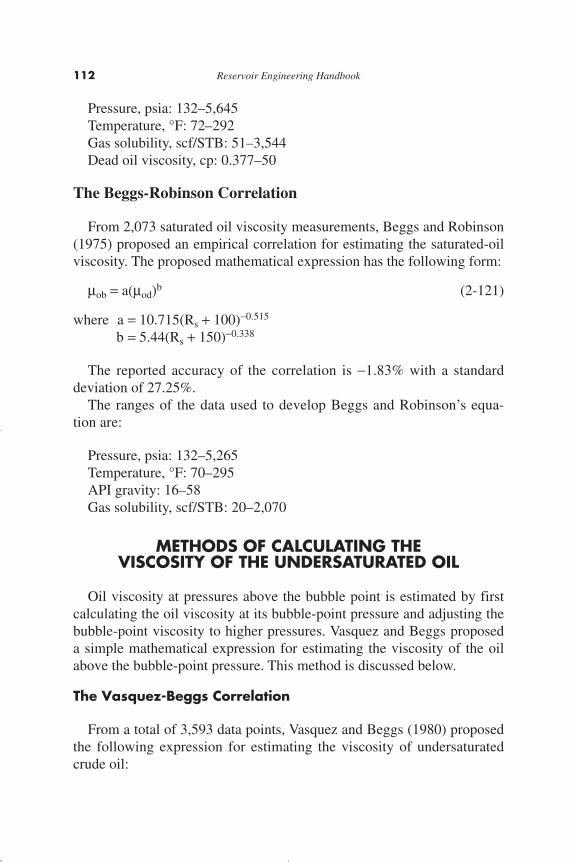
Pressure, psia: 132–5,645Temperature, °F: 72–292Gas solubility, scf/STB: 51–3,544Dead oil viscosity, cp: 0.377–50
The Beggs-Robinson Correlation
From 2,073 saturated oil viscosity measurements, Beggs and Robinson(1975) proposed an empirical correlation for estimating the saturated-oilviscosity. The proposed mathematical expression has the following form:
mob = a(mod)b (2-121)
where a = 10.715(Rs + 100)-0.515
b = 5.44(Rs + 150)-0.338
The reported accuracy of the correlation is -1.83% with a standarddeviation of 27.25%.
The ranges of the data used to develop Beggs and Robinson’s equa-tion are:
Pressure, psia: 132–5,265Temperature, °F: 70–295API gravity: 16–58Gas solubility, scf/STB: 20–2,070
METHODS OF CALCULATING THEVISCOSITY OF THE UNDERSATURATED OIL
Oil viscosity at pressures above the bubble point is estimated by firstcalculating the oil viscosity at its bubble-point pressure and adjusting thebubble-point viscosity to higher pressures. Vasquez and Beggs proposeda simple mathematical expression for estimating the viscosity of the oilabove the bubble-point pressure. This method is discussed below.
The Vasquez-Beggs Correlation
From a total of 3,593 data points, Vasquez and Beggs (1980) proposedthe following expression for estimating the viscosity of undersaturatedcrude oil:
112 Reservoir Engineering Handbook
Reservoir Eng Hndbk Ch 02b 2001-10-24 09:26 Page 112
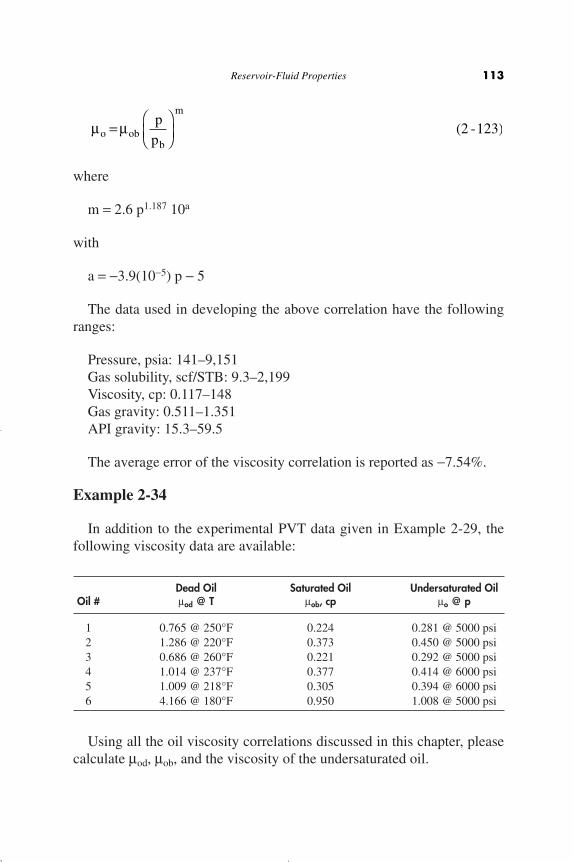
where
m = 2.6 p1.187 10a
with
a = -3.9(10-5) p - 5
The data used in developing the above correlation have the followingranges:
Pressure, psia: 141–9,151Gas solubility, scf/STB: 9.3–2,199Viscosity, cp: 0.117–148Gas gravity: 0.511–1.351API gravity: 15.3–59.5
The average error of the viscosity correlation is reported as -7.54%.
Example 2-34
In addition to the experimental PVT data given in Example 2-29, thefollowing viscosity data are available:
Dead Oil Saturated Oil Undersaturated OilOil # mod @ T mob, cp mo @ p
1 0.765 @ 250°F 0.224 0.281 @ 5000 psi2 1.286 @ 220°F 0.373 0.450 @ 5000 psi3 0.686 @ 260°F 0.221 0.292 @ 5000 psi4 1.014 @ 237°F 0.377 0.414 @ 6000 psi5 1.009 @ 218°F 0.305 0.394 @ 6000 psi6 4.166 @ 180°F 0.950 1.008 @ 5000 psi
Using all the oil viscosity correlations discussed in this chapter, pleasecalculate mod, mob, and the viscosity of the undersaturated oil.
m mo obb
mp
p=
ÊËÁ
ˆ¯
(2 -123)
Reservoir-Fluid Properties 113
Reservoir Eng Hndbk Ch 02b 2001-10-24 09:26 Page 113

Solution
Dead-oil viscosity
Oil # Measured mod Beal’s Beggs-Robinson Glaso’s
1 0.765 0.322 0.568 0.4172 0.286 0.638 1.020 0.7753 0.686 0.275 0.493 0.3634 1.014 0.545 0.917 0.7145 1.009 0.512 0.829 0.5986 4.166 4.425 4.246 4.536
AAE 44.9% 17.32% 35.26%
Saturated-oil viscosity
Oil # Measured mob Chew-Connally Beggs-Robinson
1 0.224 0.313* 0.287*2 0.373 0.426 0.3773 0.221 0.308 0.2794 0.377 0.311 0.2975 0.305 0.316 0.3006 0.950 0.842 0.689
AAE 21% 17%
*Using the measured mod.
Undersaturated-oil viscosity
Oil # Measured mo Beal’s Vasquez-Beggs
1 0.281 0.273* 0.303*2 0.45 0.437 0.4853 0.292 0.275 0.3184 0.414 0.434 0.4725 0.396 0.373 0.4176 1.008 0.945 1.016
AAE 3.8% 7.5%
Using the measured mob.
114 Reservoir Engineering Handbook
Reservoir Eng Hndbk Ch 02b 2001-10-24 09:26 Page 114

Surface/Interfacial Tension
The surface tension is defined as the force exerted on the boundarylayer between a liquid phase and a vapor phase per unit length. Thisforce is caused by differences between the molecular forces in the vaporphase and those in the liquid phase, and also by the imbalance of theseforces at the interface. The surface can be measured in the laboratory andis unusually expressed in dynes per centimeter. The surface tension is animportant property in reservoir engineering calculations and designingenhanced oil recovery projects.
Sugden (1924) suggested a relationship that correlates the surface ten-sion of a pure liquid in equilibrium with its own vapor. The correlatingparameters of the proposed relationship are molecular weight M of thepure component, the densities of both phases, and a newly introducedtemperature independent parameter Pch. The relationship is expressedmathematically in the following form:
where s is the surface tension and Pch is a temperature independent para-meter and is called the parachor.
The parachor is a dimensionless constant characteristic of a pure com-pound and is calculated by imposing experimentally measured surfacetension and density data on Equation 2-124 and solving for Pch. TheParachor values for a selected number of pure compounds are given inTable 2-1 as reported by Weinaug and Katz (1943).
Table 2-1Parachor for Pure Substances
Component Parachor Component Parachor
CO2 78.0 n-C4 189.9N2 41.0 i-C5 225.0C1 77.0 n-C5 231.5C2 108.0 n-C6 271.0C3 150.3 n-C7 312.5
i-C4 181.5 n-C8 351.5
s r r= -ÈÎÍ
˘˚
PM
ch L v( ) 4
(2 -124)
Reservoir-Fluid Properties 115
Reservoir Eng Hndbk Ch 02b 2001-10-24 09:26 Page 115
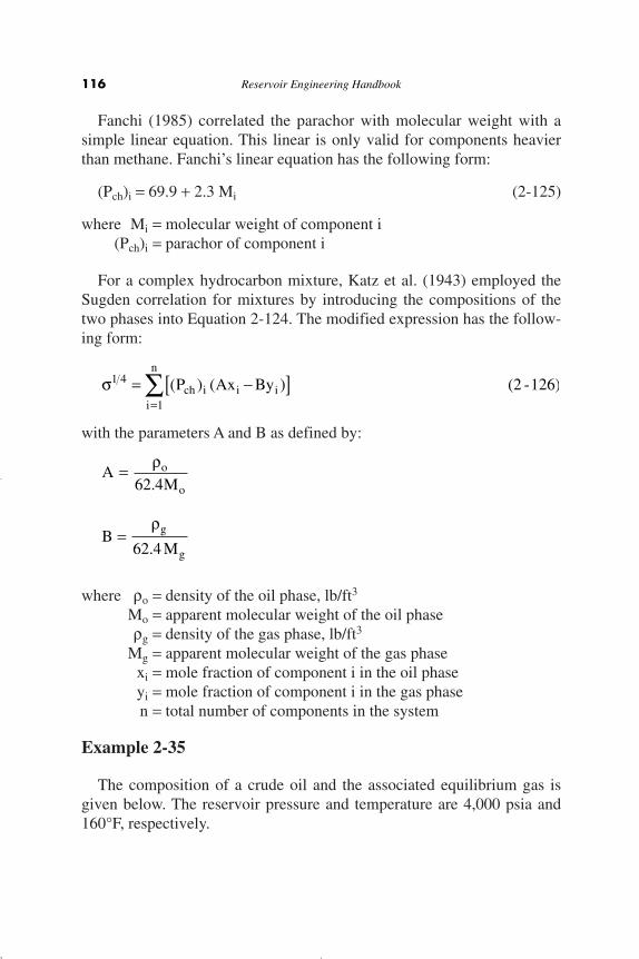
Fanchi (1985) correlated the parachor with molecular weight with asimple linear equation. This linear is only valid for components heavierthan methane. Fanchi’s linear equation has the following form:
(Pch)i = 69.9 + 2.3 Mi (2-125)
where Mi = molecular weight of component i(Pch)i = parachor of component i
For a complex hydrocarbon mixture, Katz et al. (1943) employed theSugden correlation for mixtures by introducing the compositions of thetwo phases into Equation 2-124. The modified expression has the follow-ing form:
with the parameters A and B as defined by:
where ro = density of the oil phase, lb/ft3
Mo = apparent molecular weight of the oil phaserg = density of the gas phase, lb/ft3
Mg = apparent molecular weight of the gas phasexi = mole fraction of component i in the oil phaseyi = mole fraction of component i in the gas phasen = total number of components in the system
Example 2-35
The composition of a crude oil and the associated equilibrium gas isgiven below. The reservoir pressure and temperature are 4,000 psia and160°F, respectively.
AM
BM
o
o
g
g
=
=
r
r
62 4
62 4
.
.
s1 4
1
= -[ ]=
 ( ) ( )P Ax Bych i i ii
n
(2 -126)
116 Reservoir Engineering Handbook
Reservoir Eng Hndbk Ch 02b 2001-10-24 09:26 Page 116
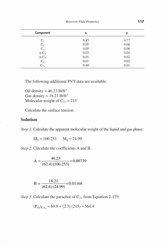
Component xi yi
C1 0.45 0.77C2 0.05 0.08C3 0.05 0.06
n-C4 0.03 0.04n-C5 0.01 0.02C6 0.01 0.02C7+ 0.40 0.01
The following additional PVT data are available:
Oil density = 46.23 lb/ft3
Gas density = 18.21 lb/ft3
Molecular weight of C7+ = 215
Calculate the surface tension.
Solution
Step 1. Calculate the apparent molecular weight of the liquid and gas phase:
Mo = 100.253 Mg = 24.99
Step 2. Calculate the coefficients A and B:
Step 3. Calculate the parachor of C7+ from Equation 2-125:
(Pch)C7+ = 69.9 + (2.3) (215) = 564.4
B = =18 2162 6 24 99
0 01168.
( . ) ( . ).
A = =46 2362 4 100 253
0 00739.
( . ) ( . ).
Reservoir-Fluid Properties 117
Reservoir Eng Hndbk Ch 02b 2001-10-24 09:26 Page 117

Step 4. Construct the following working table:
Component Pch Axi Byi Pch(Axi - Byi)
C1 77 0.00333 0.0090 -0.4361C2 108 0.00037 0.00093 -0.0605C3 150.3 0.00037 0.00070 -0.0497n-C4 189.9 0.00022 0.00047 -0.0475n-C5 231.5 0.00007 0.00023 -0.0370C6 271.0 0.000074 0.00023 -0.0423C7+ 564.4 0.00296 0.000117 1.6046
0.9315
Step 5. s = (0.9315)4 = 0.753 dynes/cm
PROPERTIES OF RESERVOIR WATER
Water Formation Volume Factor
The water formation volume factor can be calculated by the followingmathematical expression:*
Bw = A1 + A2 p + A3 p2 (2-127)
where the coefficients A1 - A3 are given by the following expression:
Ai = a1 + a2(T - 460) + a3(T - 460)2
with a1–a3 given for gas-free and gas-saturated water:
Gas-Free Water
Ai a1 a2 a3
A1 0.9947 5.8(10-6) 1.02(10-6)A2 -4.228(10-6) 1.8376(10-8) -6.77(10-11)A3 1.3(10-10) -1.3855(10-12) 4.285(10-15)
Gas-Saturated Water
Ai a1 a2 a3
A1 0.9911 6.35(10-5) 8.5(10-7)A2 -1.093(10-6) -3.497(10-9) 4.57(10-12)A3 -5.0(10-11) 6.429(10-13) -1.43(10-15)
118 Reservoir Engineering Handbook
*Hewlett-Packard H.P. 41C Petroleum Fluids PAC manual, 1982.
Reservoir Eng Hndbk Ch 02b 2001-10-24 09:26 Page 118
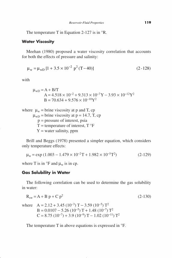
The temperature T in Equation 2-127 is in °R.
Water Viscosity
Meehan (1980) proposed a water viscosity correlation that accountsfor both the effects of pressure and salinity:
with
mwD = A + B/TA = 4.518 ¥ 10-2 + 9.313 ¥ 10-7Y - 3.93 ¥ 10-12Y2
B = 70.634 + 9.576 ¥ 10-10Y2
where mw = brine viscosity at p and T, cpmwD = brine viscosity at p = 14.7, T, cp
p = pressure of interest, psiaT = temperature of interest, T °FY = water salinity, ppm
Brill and Beggs (1978) presented a simpler equation, which considersonly temperature effects:
mw = exp (1.003 - 1.479 ¥ 10-2T + 1.982 ¥ 10-5T2) (2-129)
where T is in °F and mw is in cp.
Gas Solubility in Water
The following correlation can be used to determine the gas solubilityin water:
Rsw = A + B p + C p2 (2-130)
where A = 2.12 + 3.45 (10-3) T - 3.59 (10-5) T2
B = 0.0107 - 5.26 (10-5) T + 1.48 (10-7) T2
C = 8.75 (10-7) + 3.9 (10-9) T - 1.02 (10-11) T2
The temperature T in above equations is expressed in °F.
m mw wD p T= + ¥ --[ . ( )]1 3 5 10 402 2 (2 -128)
Reservoir-Fluid Properties 119
Reservoir Eng Hndbk Ch 02b 2001-10-24 09:26 Page 119

Water Isothermal Compressibility
Brill and Beggs (1978) proposed the following equation for estimatingwater isothermal compressibility, ignoring the corrections for dissolvedgas and solids:
Cw = (C1 + C2T + C3T2) ¥ 10-6 (2-131)
where C1 = 3.8546 - 0.000134 pC2 = -0.01052 + 4.77 ¥ 10-7 pC3 = 3.9267 ¥ 10-5 - 8.8 ¥ 10-10pT = °Fp = psia
Cw = psi-1
PROBLEMS
1. Assuming an ideal gas behavior, calculate the density of n-butane at220°F and 50 psia.
2. Show that:
3. Given the following gas:
Component Weight Fraction
C1 0.65C2 0.15C3 0.10
n-C4 0.06n-C5 0.04
Calculate:
a. Mole fraction of the gasb. Apparent molecular weightc. Specific gravityd. Specific volume at 300 psia and 120°F by assuming an ideal gas
behavior
yw M
w Mii i
i ii
=Â
( / )
( / )
120 Reservoir Engineering Handbook
Reservoir Eng Hndbk Ch 02b 2001-10-24 09:26 Page 120
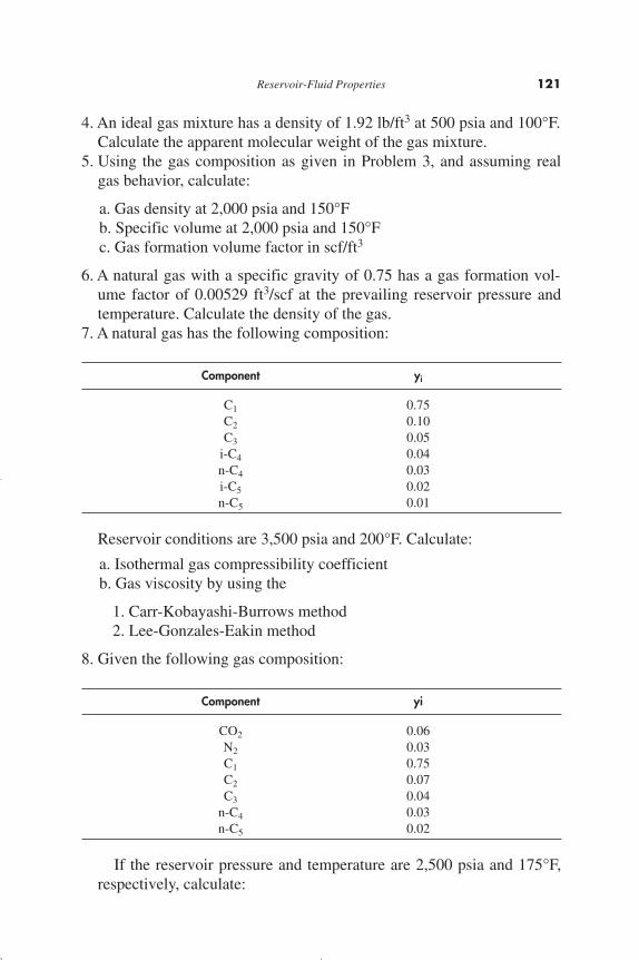
4. An ideal gas mixture has a density of 1.92 lb/ft3 at 500 psia and 100°F.Calculate the apparent molecular weight of the gas mixture.
5. Using the gas composition as given in Problem 3, and assuming realgas behavior, calculate:
a. Gas density at 2,000 psia and 150°Fb. Specific volume at 2,000 psia and 150°Fc. Gas formation volume factor in scf/ft3
6. A natural gas with a specific gravity of 0.75 has a gas formation vol-ume factor of 0.00529 ft3/scf at the prevailing reservoir pressure andtemperature. Calculate the density of the gas.
7. A natural gas has the following composition:
Component yi
C1 0.75C2 0.10C3 0.05
i-C4 0.04n-C4 0.03i-C5 0.02n-C5 0.01
Reservoir conditions are 3,500 psia and 200°F. Calculate:
a. Isothermal gas compressibility coefficientb. Gas viscosity by using the
1. Carr-Kobayashi-Burrows method2. Lee-Gonzales-Eakin method
8. Given the following gas composition:
Component yi
CO2 0.06N2 0.03C1 0.75C2 0.07C3 0.04
n-C4 0.03n-C5 0.02
If the reservoir pressure and temperature are 2,500 psia and 175°F,respectively, calculate:
Reservoir-Fluid Properties 121
Reservoir Eng Hndbk Ch 02b 2001-10-24 09:26 Page 121
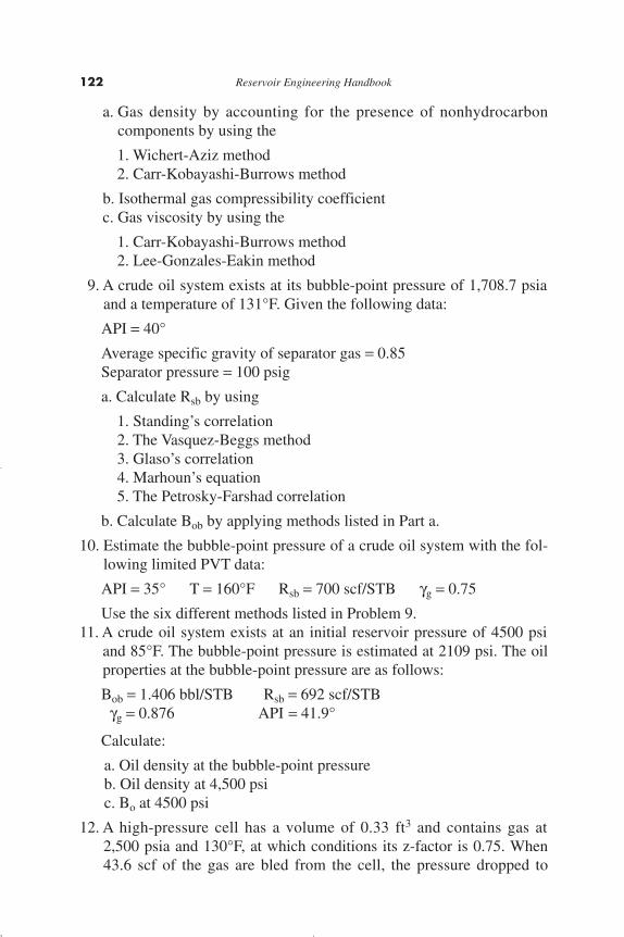
a. Gas density by accounting for the presence of nonhydrocarboncomponents by using the
1. Wichert-Aziz method2. Carr-Kobayashi-Burrows method
b. Isothermal gas compressibility coefficientc. Gas viscosity by using the
1. Carr-Kobayashi-Burrows method2. Lee-Gonzales-Eakin method
9. A crude oil system exists at its bubble-point pressure of 1,708.7 psiaand a temperature of 131°F. Given the following data:
API = 40°
Average specific gravity of separator gas = 0.85Separator pressure = 100 psig
a. Calculate Rsb by using
1. Standing’s correlation2. The Vasquez-Beggs method3. Glaso’s correlation4. Marhoun’s equation5. The Petrosky-Farshad correlation
b. Calculate Bob by applying methods listed in Part a.
10. Estimate the bubble-point pressure of a crude oil system with the fol-lowing limited PVT data:
API = 35° T = 160°F Rsb = 700 scf/STB gg = 0.75
Use the six different methods listed in Problem 9.11. A crude oil system exists at an initial reservoir pressure of 4500 psi
and 85°F. The bubble-point pressure is estimated at 2109 psi. The oilproperties at the bubble-point pressure are as follows:
Bob = 1.406 bbl/STB Rsb = 692 scf/STBgg = 0.876 API = 41.9°
Calculate:
a. Oil density at the bubble-point pressureb. Oil density at 4,500 psic. Bo at 4500 psi
12. A high-pressure cell has a volume of 0.33 ft3 and contains gas at2,500 psia and 130°F, at which conditions its z-factor is 0.75. When43.6 scf of the gas are bled from the cell, the pressure dropped to
122 Reservoir Engineering Handbook
Reservoir Eng Hndbk Ch 02b 2001-10-24 09:26 Page 122

1,000 psia, the temperature remaining at 130°F. What is the gas devi-ation factor at 1,000 psia and 130°F?
13. A hydrocarbon gas mixture with a specific gravity of 0.7 has a densi-ty of 9 lb/ft3 at the prevailing reservoir pressure and temperature. Cal-culate the gas formation volume factor in bbl/scf.
14. A gas reservoir exists at a 150°F. The gas has the following composition:
Component Mole%
C1 89C2 7C3 4
The gas expansion factor Eg was calculated as 204.648 scf/ft3 at theexisting reservoir pressure and temperature. Calculate the viscosity ofthe gas.
15. A 20 cu ft tank at a pressure of 2500 psia and 212°F contains ethanegas. How many pounds of ethane are in the tank?
16. The PVT data as shown below were obtained on a crude oil sampletaken from the Nameless Field. The initial reservoir pressure was3600 psia at 160°F. The average specific gravity of the solution gas is0.65. The reservoir contains 250 mm bbl of oil initially in place. Theoil has a bubble-point pressure of 2500 psi.a. Calculate the two-phase oil formation volume factor at:
1. 3200 psia2. 2800 psia3. 1800 psia
b. What is the initial volume of dissolved gas in the reservoir?c. Oil compressibility coefficient at 3200 psia.
Solution gas, Formation VolumePressure, scf/STB at Factor,
psia 1407 psia and 60°F bbl/STB
3600 1.3103200 1.3172800 1.3252500 567 1.3332400 554 1.3101800 436 1.2631200 337 1.210600 223 1.140200 143 1.070
Reservoir-Fluid Properties 123
Reservoir Eng Hndbk Ch 02b 2001-10-24 09:26 Page 123

17. The following PVT data were obtained from the analysis of a bottom-hole sample.
p Relative Volumepsia V/Vsat
3000 1.00002927 1.00632703 1.02862199 1.10431610 1.27861206 1.5243999 1.7399
a. Plot the Y-function versus pressure on rectangular coordinatepaper, see Equation 3-3
b. Determine the constants in the equation
Y = mp + b
by using method of least squares.c. Recalculate relative oil volume from the equation, see Equation 3-5
18. A 295-cc crude oil sample was placed in a PVT at an initial pressureof 3500 psi. The cell temperature was held at a constant temperatureof 220°F. A differential liberation test was then performed on thecrude oil sample with the recorded measurements as given below:
Vol. of Liberated Specific Gravityp, T, Total Volume, Vol. of Liquids, Gas, ofpsi °F cc cc scf Liberated Gas
3500 220 290 290 0 —3300 220 294 294 0 —
*3000 220 300 300 0 —2000 220 323.2 286.4 0.1627 0.8231000 220 375.2 271.5 0.1840 0.82314.7 60 — 179.53 0.5488 0.823
*Bubble-point pressure
Using the bore-recorded measurements and assuming an oil gravi-ty of 40° API, calculate the following PVT properties:
a. Oil formation volume factor at 3500 psi.b. Gas solubility at 3500 psi.
124 Reservoir Engineering Handbook
Reservoir Eng Hndbk Ch 02b 2001-10-24 09:26 Page 124
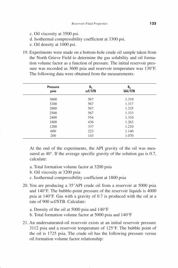
c. Oil viscosity at 3500 psi.d. Isothermal compressibility coefficient at 3300 psi.e. Oil density at 1000 psi.
19. Experiments were made on a bottom-hole crude oil sample taken fromthe North Grieve Field to determine the gas solubility and oil forma-tion volume factor as a function of pressure. The initial reservoir pres-sure was recorded as 3600 psia and reservoir temperature was 130°F.The following data were obtained from the measurements:
Pressure RS Bopsia scf/STB bbl/STB
3600 567 1.3103200 567 1.3172800 567 1.3252500 567 1.3332400 554 1.3101800 436 1.2631200 337 1.210600 223 1.140200 143 1.070
At the end of the experiments, the API gravity of the oil was mea-sured as 40°. If the average specific gravity of the solution gas is 0.7,calculate:
a. Total formation volume factor at 3200 psiab. Oil viscosity at 3200 psiac. Isothermal compressibility coefficient at 1800 psia
20. You are producing a 35°API crude oil from a reservoir at 5000 psiaand 140°F. The bubble-point pressure of the reservoir liquids is 4000psia at 140°F. Gas with a gravity of 0.7 is produced with the oil at arate of 900 scf/STB. Calculate:
a. Density of the oil at 5000 psia and 140°Fb. Total formation volume factor at 5000 psia and 140°F
21. An undersaturated-oil reservoir exists at an initial reservoir pressure3112 psia and a reservoir temperature of 125°F. The bubble point ofthe oil is 1725 psia. The crude oil has the following pressure versusoil formation volume factor relationship:
Reservoir-Fluid Properties 125
Reservoir Eng Hndbk Ch 02b 2001-10-24 09:26 Page 125
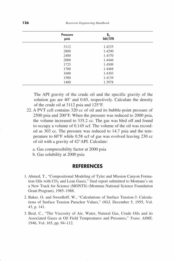
Pressure Bopsia bbl/STB
3112 1.42352800 1.42902400 1.43702000 1.44461725 1.45091700 1.44681600 1.43031500 1.41391400 1.3978
The API gravity of the crude oil and the specific gravity of thesolution gas are 40° and 0.65, respectively. Calculate the densityof the crude oil at 3112 psia and 125°F.
22. A PVT cell contains 320 cc of oil and its bubble-point pressure of2500 psia and 200°F. When the pressure was reduced to 2000 psia,the volume increased to 335.2 cc. The gas was bled off and foundto occupy a volume of 0.145 scf. The volume of the oil was record-ed as 303 cc. The pressure was reduced to 14.7 psia and the tem-perature to 60°F while 0.58 scf of gas was evolved leaving 230 ccof oil with a gravity of 42°API. Calculate:
a. Gas compressibility factor at 2000 psiab. Gas solubility at 2000 psia
REFERENCES
1. Ahmed, T., “Compositional Modeling of Tyler and Mission Canyon Forma-tion Oils with CO2 and Lean Gases,” final report submitted to Montana’s ona New Track for Science (MONTS) (Montana National Science FoundationGrant Program), 1985–1988.
2. Baker, O. and Swerdloff, W., “Calculations of Surface Tension-3: Calcula-tions of Surface Tension Parachor Values,” OGJ, December 5, 1955, Vol.43, p. 141.
3. Beal, C., “The Viscosity of Air, Water, Natural Gas, Crude Oils and itsAssociated Gases at Oil Field Temperatures and Pressures,” Trans. AIME,1946, Vol. 165, pp. 94–112.
126 Reservoir Engineering Handbook
Reservoir Eng Hndbk Ch 02b 2001-10-24 09:26 Page 126

4. Beggs, H. D. and Robinson, J. R., “Estimating the Viscosity of Crude OilSystems,” JPT, September 1975, pp. 1140–1141.
5. Brill, J. and Beggs, H., Two-Phase Flow in Pipes. Tulsa, OK: The Universi-ty of Tulsa, 1978.
6. Brown, et al., “Natural Gasoline and the Volatile Hydrocarbons,” Tulsa:NGAA, 1948.
7. Carr, N., Kobayashi, R., and Burrows, D., “Viscosity of Hydrocarbon GasesUnder Pressure,” Trans. AIME, 1954, Vol. 201, pp. 270–275.
8. Chew, J., and Connally, Jr., C. A., “A Viscosity Correlation for Gas-Saturat-ed Crude Oils,” Trans. AIME, 1959, Vol. 216, pp. 23–25.
9. Dean, D. E., and Stiel, L. I., “The Viscosity of Non-polar Gas Mixtures atModerate and High Pressure,” AIChE Jour., 1958, Vol. 4, pp. 430–436.
10. Dempsey, J. R., “Computer Routine Treats Gas Viscosity as a Variable,” Oiland Gas Journal, Aug. 16, 1965, pp. 141–143.
11. Dranchuk, P. M., and Abu-Kassem, J. H., “Calculation of Z-factors for Nat-ural Gases Using Equations-of-State,” JCPT, July–Sept., 1975, pp. 34–36.
12. Dranchuk, P. M., Purvis, R. A., and Robinson, D. B., “Computer Calcula-tions of Natural Gas Compressibility Factors Using the Standing and KatzCorrelation,” Inst. Of Petroleum Technical Series, No. IP 74-008, 1974.
13. Fanchi, J. R., “Calculation of Parachors for Composition Simulation,” JPT,November 1985, pp. 2049–2050.
14. Glaso, O., “Generalized Pressure-Volume-Temperature Correlations,” JPT,May 1980, pp. 785–795.
15. Hall, K. R., and Yarborough, L., “A New Equation-of-State for Z-factor Cal-culations,” Oil and Gas Journal, June 18, 1973, pp. 82–92.
16. Hankinson, R. W., Thomas, L. K., and Phillips, K. A., “Predict Natural GasProperties,” Hydrocarbon Processing, April 1969, pp. 106–108.
17. Kay, W. B., “Density of Hydrocarbon Gases and Vapor,” Industrial andEngineering Chemistry, 1936, Vol. 28, pp. 1014–1019.
18. Lee, A. L., Gonzalez, M. H., and Eakin, B. E., “The Viscosity of NaturalGases,” JTP, August 1966, pp. 997–1000.
19. Marhoun, M. A., “PVT Correlation for Middle East Crude Oils,” JPT, May1988, pp. 650–665.
20. Mattar, L. G., Brar, S., and Aziz, K., “Compressibility of Natural Gases,”Journal of Canadian Petroleum Technology, October–November 1975, pp.77–80.
Reservoir-Fluid Properties 127
Reservoir Eng Hndbk Ch 02b 2001-10-24 09:26 Page 127

21. Meehan, D. N., “A Correlation for Water Compressibility,” Petroleum Engi-neer, November 1980, pp. 125–126.
22. Papay, J., “A Termelestechnologiai Parameterek Valtozasa a GazlelepkMuvelese Soran,” OGIL MUSZ, Tud, Kuzl., Budapest, 1968, pp. 267–273.
23. Petrosky, G. E., and Farshad, F., “Pressure-Volume-Temperature Correla-tions for Gulf of Mexico Crude Oils,” SPE Paper 26644, presented at the68th Annual Technical Conference of the SPE in Houston, Texas, 3–6 Octo-ber, 1993.
24. Standing, M. B., Volumetric and Phase Behavior of Oil Field HydrocarbonSystems, pp. 125–126. Dallas: Society of Petroleum Engineers, 1977.
25. Standing, M. B. and Katz, D. L., “Density of Natural Gases,” Trans. AIME,1942, Vol. 146, pp. 140–149.
26. Stewart, W. F., Burkhard, S. F., and Voo, D., “Prediction of Pseudo-CriticalParameters for Mixtures,” paper presented at the AIChE Meeting, KansasCity, MO, 1959.
27. Sugden, S., “The Variation of Surface Tension, VI. The Variation of SurfaceTension with Temperature and Some Related Functions,” J. Chem. Soc.,1924, Vol. 125, pp. 32–39.
28. Sutton, R. P., “Compressibility Factors for High-Molecular-Weight Reser-voir Gases,” SPE Paper 14265, presented at the 60th Annual Technical Con-ference and Exhibition of the Society of Petroleum Engineers, Las Vegas,Sept. 22–25, 1985.
29. Sutton, R. P., and Farshad, F. F., “Evaluation of Empirically Derived PVTProperties for Gulf of Mexico Crude Oils,” SPE Paper 13172, presented atthe 59th Annual Technical Conference, Houston, Texas, 1984.
30. Takacs, G., “Comparisons Made for Computer Z-Factor Calculation,” Oiland Gas Journal, Dec. 20, 1976, pp. 64–66.
31. Trube, A. S., “Compressibility of Undersaturated Hydrocarbon ReservoirFluids,” Trans. AIME, 1957, Vol. 210, pp. 341–344.
32. Trube, A. S., “Compressibility of Natural Gases,” Trans AIME, 1957, Vol.210, pp. 355–357.
33. Vasquez, M., and Beggs, D., “Correlations for Fluid Physical Properties Pre-diction,” JPT, June 1980, pp. 968–970.
128 Reservoir Engineering Handbook
Reservoir Eng Hndbk Ch 02b 2001-10-24 09:26 Page 128

34. Weinaug, C., and Katz, D. L., “Surface Tension of Methane-Propane Mix-tures,” Ind. Eng. Chem., 1943, Vol. 25, pp. 35–43.
35. Wichert, E., and Aziz, K., “Calculation of Z’s for Sour Gases,” HydrocarbonProcessing, 1972, Vol. 51, No. 5, pp. 119–122.
36. Yarborough, L., and Hall, K. R., “How to Solve Equation-of-State for Z-fac-tors,” Oil and Gas Journal, Feb 18, 1974, pp. 86–88.
Reservoir-Fluid Properties 129
Reservoir Eng Hndbk Ch 02b 2001-10-24 09:26 Page 129

The material of which a petroleum reservoir rock may be composedcan range from very loose and unconsolidated sand to a very hard anddense sandstone, limestone, or dolomite. The grains may be bondedtogether with a number of materials, the most common of which are sili-ca, calcite, or clay. Knowledge of the physical properties of the rock andthe existing interaction between the hydrocarbon system and the forma-tion is essential in understanding and evaluating the performance of agiven reservoir.
Rock properties are determined by performing laboratory analyses oncores from the reservoir to be evaluated. The cores are removed from thereservoir environment, with subsequent changes in the core bulk volume,pore volume, reservoir fluid saturations, and, sometimes, formation wet-tability. The effect of these changes on rock properties may range fromnegligible to substantial, depending on characteristics of the formationand property of interest, and should be evaluated in the testing program.
There are basically two main categories of core analysis tests that areperformed on core samples regarding physical properties of reservoirrocks. These are:
Routine core analysis tests
• Porosity• Permeability• Saturation
183
C H A P T E R 4
FUNDAMENTALS OFROCK PROPERTIES
Reservoir Eng Hndbk Ch 04a 2001-10-24 09:36 Page 183
Special tests
• Overburden pressure• Capillary pressure• Relative permeability• Wettability• Surface and interfacial tension
The above rock property data are essential for reservoir engineeringcalculations as they directly affect both the quantity and the distributionof hydrocarbons and, when combined with fluid properties, control theflow of the existing phases (i.e., gas, oil, and water) within the reservoir.
POROSITY
The porosity of a rock is a measure of the storage capacity (pore vol-ume) that is capable of holding fluids. Quantitatively, the porosity is theratio of the pore volume to the total volume (bulk volume). This impor-tant rock property is determined mathematically by the following gener-alized relationship:
where f = porosity
As the sediments were deposited and the rocks were being formed dur-ing past geological times, some void spaces that developed became iso-lated from the other void spaces by excessive cementation. Thus, manyof the void spaces are interconnected while some of the pore spaces arecompletely isolated. This leads to two distinct types of porosity, namely:
• Absolute porosity• Effective porosity
Absolute porosity
The absolute porosity is defined as the ratio of the total pore space inthe rock to that of the bulk volume. A rock may have considerableabsolute porosity and yet have no conductivity to fluid for lack of pore
f =pore volumebulk volume
184 Reservoir Engineering Handbook
Reservoir Eng Hndbk Ch 04a 2001-10-24 09:36 Page 184
interconnection. The absolute porosity is generally expressed mathemati-cally by the following relationships:
or
where fa = absolute porosity.
Effective porosity
The effective porosity is the percentage of interconnected pore spacewith respect to the bulk volume, or
where f = effective porosity.
The effective porosity is the value that is used in all reservoir engi-neering calculations because it represents the interconnected pore spacethat contains the recoverable hydrocarbon fluids.
Porosity may be classified according to the mode of origin as originalinduced.
The original porosity is that developed in the deposition of the materi-al, while induced porosity is that developed by some geologic processsubsequent to deposition of the rock. The intergranular porosity of sand-stones and the intercrystalline and oolitic porosity of some limestones typ-ify original porosity. Induced porosity is typified by fracture developmentas found in shales and limestones and by the slugs or solution cavitiescommonly found in limestones. Rocks having original porosity are moreuniform in their characteristics than those rocks in which a large part ofthe porosity is included. For direct quantitative measurement of porosity,reliance must be placed on formation samples obtained by coring.
Since effective porosity is the porosity value of interest to the petrole-um engineer, particular attention should be paid to the methods used to
f =interconnected pore volume
bulk volume(4 - 3)
a =bulk volume grain volume
bulk volumef -
(4 - 2)
a =total pore volume
bulk volumef (4 -1)
Fundamentals of Rock Properties 185
Reservoir Eng Hndbk Ch 04a 2001-10-24 09:36 Page 185
determine porosity. For example, if the porosity of a rock sample wasdetermined by saturating the rock sample 100 percent with a fluid ofknown density and then determining, by weighing, the increased weightdue to the saturating fluid, this would yield an effective porosity measure-ment because the saturating fluid could enter only the interconnected porespaces. On the other hand, if the rock sample were crushed with a mortarand pestle to determine the actual volume of the solids in the core sample,then an absolute porosity measurement would result because the identityof any isolated pores would be lost in the crushing process.
One important application of the effective porosity is its use in deter-mining the original hydrocarbon volume in place. Consider a reservoirwith an areal extent of A acres and an average thickness of h feet. Thetotal bulk volume of the reservoir can be determined from the followingexpressions:
Bulk volume = 43,560 Ah, ft3 (4-4)
or
Bulk volume = 7,758 Ah, bbl (4-5)
where A = areal extent, acresh = average thickness
The reservoir pore volume PV can then be determined by combiningEquations 4-4 and 4-5 with 4-3. Expressing the reservoir pore volume incubic feet gives:
PV = 43,560 Ahf, ft3 (4-6)
Expressing the reservoir pore volume in barrels gives:
PV = 7,758 Ahf, bbl (4-7)
Example 4-1
An oil reservoir exists at its bubble-point pressure of 3000 psia andtemperature of 160°F. The oil has an API gravity of 42° and gas-oil ratioof 600 scf/STB. The specific gravity of the solution gas is 0.65. The fol-lowing additional data are also available:
186 Reservoir Engineering Handbook
Reservoir Eng Hndbk Ch 04a 2001-10-24 09:36 Page 186
• Reservoir area = 640 acres• Average thickness = 10 ft• Connate water saturation = 0.25• Effective porosity = 15%
Calculate the initial oil in place in STB.
Solution
Step 1. Determine the specific gravity of the stock-tank oil from Equation2-68.
Step 2. Calculate the initial oil formation volume factor by applyingStanding’s equation, i.e., Equation 2-85, to give:
Step 3. Calculate the pore volume from Equation 4-7.
Pore volume = 7758 (640) (10) (0.15) = 7,447,680 bbl
Step 4. Calculate the initial oil in place.
Initial oil in place = 12,412,800 (1 - 0.25)/1.306 = 4,276,998 STB
The reservoir rock may generally show large variations in porosityvertically but does not show very great variations in porosity parallel tothe bedding planes. In this case, the arithmetic average porosity or thethickness-weighted average porosity is used to describe the averagereservoir porosity. A change in sedimentation or depositional conditions,however, can cause the porosity in one portion of the reservoir to begreatly different from that in another area. In such cases, the areal-weighted average or the volume-weighted average porosity is used tocharacterize the average rock porosity. These averaging techniques areexpressed mathematically in the following forms:
ob = 0.9759 + 0.00012 6000.65
0.8156ÊËÁ
ˆ¯
0.5
+ 1.25 (160)È
ÎÍÍ
˘
˚˙˙
1.2
=1.306 bbl /STB
o =141.5
42 + 131.5= 0.8156g
Fundamentals of Rock Properties 187
Reservoir Eng Hndbk Ch 04a 2001-10-24 09:36 Page 187
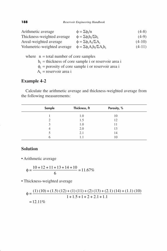
Arithmetic average f = Sfi/n (4-8)Thickness-weighted average f = Sfihi/Shi (4-9)Areal-weighted average f = SfiAi/SAi (4-10) Volumetric-weighted average f = SfiAihi/SAihi (4-11)
where n = total number of core sampleshi = thickness of core sample i or reservoir area i fi = porosity of core sample i or reservoir area iAi = reservoir area i
Example 4-2
Calculate the arithmetic average and thickness-weighted average fromthe following measurements:
Sample Thickness, ft Porosity, %
1 1.0 102 1.5 123 1.0 114 2.0 135 2.1 146 1.1 10
Solution
• Arithmetic average
• Thickness-weighted average
f =(1) (10) + (1.5) (12) + (1) (11) + (2) (13) + (2.1) (14) + (1.1) (10)
1 + 1.5 + 1 + 2 + 2.1 + 1.1= 12.11%
f =10 + 12 + 11 + 13 + 14 + 10
6= 11.67%
188 Reservoir Engineering Handbook
Reservoir Eng Hndbk Ch 04a 2001-10-24 09:36 Page 188

SATURATION
Saturation is defined as that fraction, or percent, of the pore volumeoccupied by a particular fluid (oil, gas, or water). This property isexpressed mathematically by the following relationship:
Applying the above mathematical concept of saturation to each reser-voir fluid gives
where So = oil saturationSg = gas saturationSw = water saturation
Thus, all saturation values are based on pore volume and not on thegross reservoir volume.
The saturation of each individual phase ranges between zero to 100percent. By definition, the sum of the saturations is 100%, therefore
Sg + So + Sw = 1.0 (4 -15)
The fluids in most reservoirs are believed to have reached a state ofequilibrium and, therefore, will have become separated according to their
wS =volume of water
pore volume(4 -14)
gS =volume of gaspore volume
(4 -13)
oS =volume of oilpore volume
(4 -12)
fluid saturationtotal volume of the fluid
pore volume=
Fundamentals of Rock Properties 189
Reservoir Eng Hndbk Ch 04a 2001-10-24 09:36 Page 189

density, i.e., oil overlain by gas and underlain by water. In addition to thebottom (or edge) water, there will be connate water distributed through-out the oil and gas zones. The water in these zones will have beenreduced to some irreducible minimum. The forces retaining the water inthe oil and gas zones are referred to as capillary forces because they areimportant only in pore spaces of capillary size.
Connate (interstitial) water saturation Swc is important primarilybecause it reduces the amount of space available between oil and gas. Itis generally not uniformly distributed throughout the reservoir but varieswith permeability, lithology, and height above the free water table.
Another particular phase saturation of interest is called the critical satu-ration and it is associated with each reservoir fluid. The definition and thesignificance of the critical saturation for each phase is described below.
Critical oil saturation, Soc
For the oil phase to flow, the saturation of the oil must exceed a certainvalue which is termed critical oil saturation. At this particular saturation,the oil remains in the pores and, for all practical purposes, will not flow.
Residual oil saturation, Sor
During the displacing process of the crude oil system from the porousmedia by water or gas injection (or encroachment) there will be someremaining oil left that is quantitatively characterized by a saturationvalue that is larger than the critical oil saturation. This saturation value iscalled the residual oil saturation, Sor. The term residual saturation is usu-ally associated with the nonwetting phase when it is being displaced by awetting phase.
Movable oil saturation, Som
Movable oil saturation Som is another saturation of interest and isdefined as the fraction of pore volume occupied by movable oil asexpressed by the following equation:
Som = 1 - Swc - Soc
where Swc = connate water saturationSoc = critical oil saturation
190 Reservoir Engineering Handbook
Reservoir Eng Hndbk Ch 04a 2001-10-24 09:36 Page 190
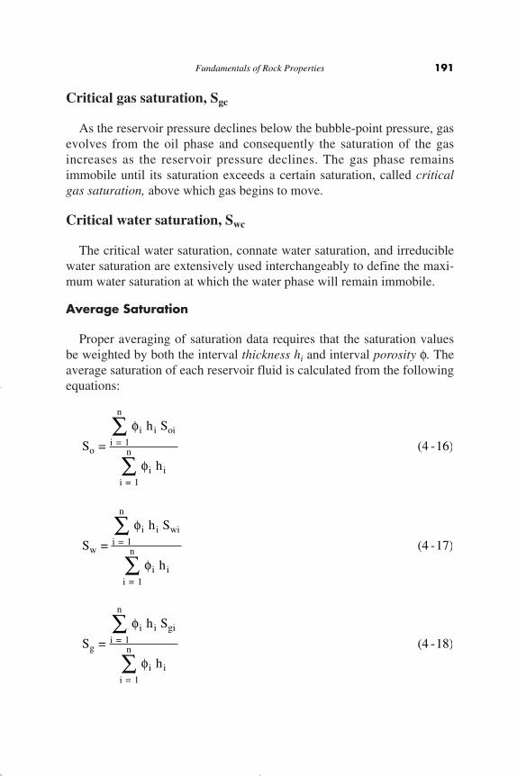
Critical gas saturation, Sgc
As the reservoir pressure declines below the bubble-point pressure, gasevolves from the oil phase and consequently the saturation of the gasincreases as the reservoir pressure declines. The gas phase remainsimmobile until its saturation exceeds a certain saturation, called criticalgas saturation, above which gas begins to move.
Critical water saturation, Swc
The critical water saturation, connate water saturation, and irreduciblewater saturation are extensively used interchangeably to define the maxi-mum water saturation at which the water phase will remain immobile.
Average Saturation
Proper averaging of saturation data requires that the saturation valuesbe weighted by both the interval thickness hi and interval porosity f. Theaverage saturation of each reservoir fluid is calculated from the followingequations:
S =
h S
hg
i = 1
n
i i gi
i = 1
n
i i
Â
Â
f
f(4 -18)
S =
h S
hw
i = 1
n
i i wi
i = 1
n
i i
Â
Â
f
f(4 -17)
S =
h S
ho
i = 1
n
i i oi
i = 1
n
i i
Â
Â
f
f(4 -16)
Fundamentals of Rock Properties 191
Reservoir Eng Hndbk Ch 04a 2001-10-24 09:36 Page 191

where the subscript i refers to any individual measurement and hi repre-sents the depth interval to which fi , Soi, Sgi, and Swi apply.
Example 4-3
Calculate average oil and connate water saturation from the followingmeasurements:
Sample hi, ft f, % So, % Swc, %
1 1.0 10 75 252 1.5 12 77 233 1.0 11 79 214 2.0 13 74 265 2.1 14 78 226 1.1 10 75 25
Solution
Construct the following table and calculate the average saturation forthe oil and water phase:
Sample hi, ft f fh So Sofh Swc Swcfh
1 1.0 .10 .100 .75 .0750 .25 .02502 1.5 .12 .180 .77 .1386 .23 .04143 1.0 .11 .110 .79 .0869 .21 .02314 2.0 .13 .260 .74 .1924 .26 .06765 2.1 .14 .294 .78 .2293 .22 .06476 1.1 .10 .110 .75 .0825 .25 .0275
1.054 0.8047 0.2493
Calculate average oil saturation by applying Equation 4-16:
Calculate average water saturation by applying Equation 4-17:
wS =0.24931.054
= 0.2365
oS =.80471.054
= 0.7635
192 Reservoir Engineering Handbook
Reservoir Eng Hndbk Ch 04a 2001-10-24 09:36 Page 192

WETTABILITY
Wettability is defined as the tendency of one fluid to spread on oradhere to a solid surface in the presence of other immiscible fluids. Theconcept of wettability is illustrated in Figure 4-1. Small drops of three liq-uids—mercury, oil, and water—are placed on a clean glass plate. Thethree droplets are then observed from one side as illustrated in Figure 4-1.It is noted that the mercury retains a spherical shape, the oil droplet devel-ops an approximately hemispherical shape, but the water tends to spreadover the glass surface.
The tendency of a liquid to spread over the surface of a solid is an indi-cation of the wetting characteristics of the liquid for the solid. This spread-ing tendency can be expressed more conveniently by measuring the angleof contact at the liquid-solid surface. This angle, which is always mea-sured through the liquid to the solid, is called the contact angle q.
The contact angle q has achieved significance as a measure of wetta-bility. As shown in Figure 4-1, as the contact angle decreases, the wettingcharacteristics of the liquid increase. Complete wettability would be evi-denced by a zero contact angle, and complete nonwetting would be evi-denced by a contact angle of 180°. There have been various definitions ofintermediate wettability but, in much of the published literature, contactangles of 60° to 90° will tend to repel the liquid.
The wettability of reservoir rocks to the fluids is important in that thedistribution of the fluids in the porous media is a function of wettability.Because of the attractive forces, the wetting phase tends to occupy thesmaller pores of the rock and the nonwetting phase occupies the moreopen channels.
Fundamentals of Rock Properties 193
Figure 4-1. Illustration of wettability.
Reservoir Eng Hndbk Ch 04a 2001-10-24 09:36 Page 193
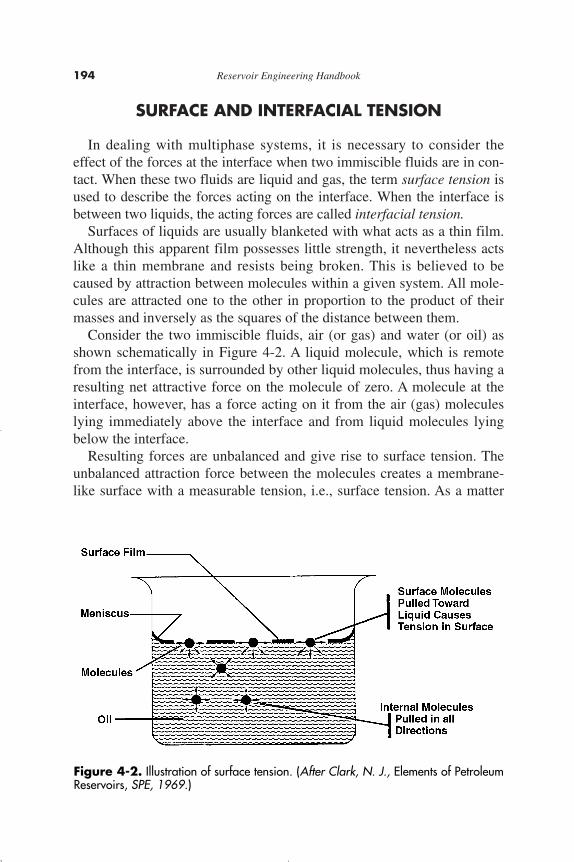
SURFACE AND INTERFACIAL TENSION
In dealing with multiphase systems, it is necessary to consider theeffect of the forces at the interface when two immiscible fluids are in con-tact. When these two fluids are liquid and gas, the term surface tension isused to describe the forces acting on the interface. When the interface isbetween two liquids, the acting forces are called interfacial tension.
Surfaces of liquids are usually blanketed with what acts as a thin film.Although this apparent film possesses little strength, it nevertheless actslike a thin membrane and resists being broken. This is believed to becaused by attraction between molecules within a given system. All mole-cules are attracted one to the other in proportion to the product of theirmasses and inversely as the squares of the distance between them.
Consider the two immiscible fluids, air (or gas) and water (or oil) asshown schematically in Figure 4-2. A liquid molecule, which is remotefrom the interface, is surrounded by other liquid molecules, thus having aresulting net attractive force on the molecule of zero. A molecule at theinterface, however, has a force acting on it from the air (gas) moleculeslying immediately above the interface and from liquid molecules lyingbelow the interface.
Resulting forces are unbalanced and give rise to surface tension. Theunbalanced attraction force between the molecules creates a membrane-like surface with a measurable tension, i.e., surface tension. As a matter
194 Reservoir Engineering Handbook
Figure 4-2. Illustration of surface tension. (After Clark, N. J., Elements of PetroleumReservoirs, SPE, 1969.)
Reservoir Eng Hndbk Ch 04a 2001-10-24 09:36 Page 194

of fact, if carefully placed, a needle will float on the surface of the liquid,supported by the thin membrane even though it is considerably moredense than the liquid.
The surface or interfacial tension has the units of force per unit oflength, e.g., dynes/cm, and is usually denoted by the symbol s.
If a glass capillary tube is placed in a large open vessel containingwater, the combination of surface tension and wettability of tube to waterwill cause water to rise in the tube above the water level in the containeroutside the tube as shown in Figure 4-3.
The water will rise in the tube until the total force acting to pull theliquid upward is balanced by the weight of the column of liquid being
Fundamentals of Rock Properties 195
Figure 4-3. Pressure relations in capillary tubes.
Reservoir Eng Hndbk Ch 04a 2001-10-24 09:36 Page 195

supported in the tube. Assuming the radius of the capillary tube is r, thetotal upward force Fup, which holds the liquid up, is equal to the force perunit length of surface times the total length of surface, or
Fup = (2pr) (sgw) (cos q) (4-19)
where sgw = surface tension between air (gas) and water (oil),dynes/cm
q = contact angler = radius, cm
The upward force is counteracted by the weight of the water, which isequivalent to a downward force of mass times acceleration, or
Fdown = pr2 h (rw - rair) g (4 -20)
where h = height to which the liquid is held, cmg = acceleration due to gravity, cm/sec2
rw = density of water, gm/cm3
rair = density of gas, gm/cm3
Because the density of air is negligible in comparison with the densityof water, Equation 4-20 is reduced to:
Fdown = p r2 rwg (4 -21)
Equating Equation 4-19 with 4-21 and solving for the surface tensiongives:
The generality of Equations 4-19 through 4-22 will not be lost byapplying them to the behavior of two liquids, i.e., water and oil. Becausethe density of oil is not negligible, Equation 4-22 becomes
where ro = density of oil, gm/cm3
sow = interfacial tension between the oil and the water, dynes/cm
oww o=
r h g ( )
2s
r rq-
cos(4 - 23)
gww=
r h g
2s
rqcos
(4 - 22)
196 Reservoir Engineering Handbook
Reservoir Eng Hndbk Ch 04a 2001-10-24 09:36 Page 196

CAPILLARY PRESSURE
The capillary forces in a petroleum reservoir are the result of the com-bined effect of the surface and interfacial tensions of the rock and fluids,the pore size and geometry, and the wetting characteristics of the system.Any curved surface between two immiscible fluids has the tendency tocontract into the smallest possible area per unit volume. This is truewhether the fluids are oil and water, water and gas (even air), or oil andgas. When two immiscible fluids are in contact, a discontinuity in pres-sure exists between the two fluids, which depends upon the curvature ofthe interface separating the fluids. We call this pressure difference thecapillary pressure and it is referred to by pc.
The displacement of one fluid by another in the pores of a porousmedium is either aided or opposed by the surface forces of capillary pres-sure. As a consequence, in order to maintain a porous medium partiallysaturated with nonwetting fluid and while the medium is also exposed towetting fluid, it is necessary to maintain the pressure of the nonwettingfluid at a value greater than that in the wetting fluid.
Denoting the pressure in the wetting fluid by pw and that in the non-wetting fluid by pnw, the capillary pressure can be expressed as:
Capillary pressure = (pressure of the nonwetting phase) - (pressure ofthe wetting phase)
pc = pnw - pw (4-24)
That is, the pressure excess in the nonwetting fluid is the capillarypressure, and this quantity is a function of saturation. This is the definingequation for capillary pressure in a porous medium.
There are three types of capillary pressure:
• Water-oil capillary pressure (denoted as Pcwo)• Gas-oil capillary pressure (denoted as Pcgo)• Gas-water capillary pressure (denoted as Pcgw)
Applying the mathematical definition of the capillary pressure asexpressed by Equation 4-24, the three types of the capillary pressure canbe written as:
pcwo = po - pw
Fundamentals of Rock Properties 197
Reservoir Eng Hndbk Ch 04a 2001-10-24 09:36 Page 197

pcgo = pg - po
pcgw = pg - pw
where pg, po, and pw represent the pressure of gas, oil, and water, respec-tively.
If all the three phases are continuous, then:
pcgw = pcgo + pcwo
Referring to Figure 4-3, the pressure difference across the interfacebetween Points 1 and 2 is essentially the capillary pressure, i.e.:
pc = p1 - p2 (4-25)
The pressure of the water phase at Point 2 is equal to the pressure atpoint 4 minus the head of the water, or:
p2 = p4 - ghrw (4-26)
The pressure just above the interface at Point 1 represents the pressureof the air and is given by:
p1 = p3 - ghrair (4-27)
It should be noted that the pressure at Point 4 within the capillary tubeis the same as that at Point 3 outside the tube. Subtracting Equation 4-26from 4-27 gives:
pc = gh (rw - rair) = ghDr (4-28)
where Dr is the density difference between the wetting and nonwettingphase. The density of the air (gas) is negligible in comparison with thewater density.
In practical units, Equation 4-28 can be expressed as:
where pc = capillary pressure, psih = capillary rise, ft
Dr = density difference, lb/ft3
cp =h
144ÊË
ˆ¯ D r
198 Reservoir Engineering Handbook
Reservoir Eng Hndbk Ch 04a 2001-10-24 09:36 Page 198
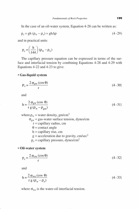
In the case of an oil-water system, Equation 4-28 can be written as:
pc = gh (rw - ro) = ghDr (4 -29)
and in practical units
The capillary pressure equation can be expressed in terms of the sur-face and interfacial tension by combining Equations 4-28 and 4-29 withEquations 4-22 and 4-23 to give:
• Gas-liquid system
and
where rw = water density, gm/cm3
sgw = gas-water surface tension, dynes/cmr = capillary radius, cm
q = contact angleh = capillary rise, cmg = acceleration due to gravity, cm/sec2
pc = capillary pressure, dynes/cm2
• Oil-water system
and
where swo is the water-oil interfacial tension.
h =2 ( )r g ( )
wo
w o
s qr r
cos-
(4 - 33)
cowp =
2 ( )r
s qcos(4 - 32)
h =2 ( )
r g ( )gw
w gas
s qr r
cos
-(4 - 31)
cgw
P =2 ( )
r
s qcos(4 - 30)
c w op =h
144
ÊË
ˆ¯ -( )r r
Fundamentals of Rock Properties 199
Reservoir Eng Hndbk Ch 04a 2001-10-24 09:36 Page 199
Example 4-4
Calculate the pressure difference, i.e., capillary pressure, and capillaryrise in an oil-water system from the following data:
q = 30° rw = 1.0 gm/cm3 ro = 0.75 gm/cm3
r = 10-4 cm sow = 25 dynes/cm
Solution
Step 1. Apply Equation 4-32 to give
Since 1 dyne/cm2 = 1.45 ¥ 10B5 psi, then
pc = 6.28 psi
This result indicates that the oil-phase pressure is 6.28 psihigher than the water-phase pressure.
Step 2. Calculate the capillary rise by applying Equation 4-33.
Capillary Pressure of Reservoir Rocks
The interfacial phenomena described above for a single capillary tubealso exist when bundles of interconnected capillaries of varying sizes existin a porous medium. The capillary pressure that exists within a porousmedium between two immiscible phases is a function of the interfacialtensions and the average size of the capillaries which, in turn, controls thecurvature of the interface. In addition, the curvature is also a function ofthe saturation distribution of the fluids involved.
Laboratory experiments have been developed to simulate the displac-ing forces in a reservoir in order to determine the magnitude of the capil-lary forces in a reservoir and, thereby, determine the fluid saturation dis-
h =(2) (25) ( 30 )
(0.0001) (980.7) (1.0 0.75)= 1766 cm = 75.9 ft
cos ∞-
c5p =
(2) (25) ( 30 )0.0001
= 4.33 10 dynes/cmcos ∞ ¥ 2
200 Reservoir Engineering Handbook
Reservoir Eng Hndbk Ch 04a 2001-10-24 09:36 Page 200
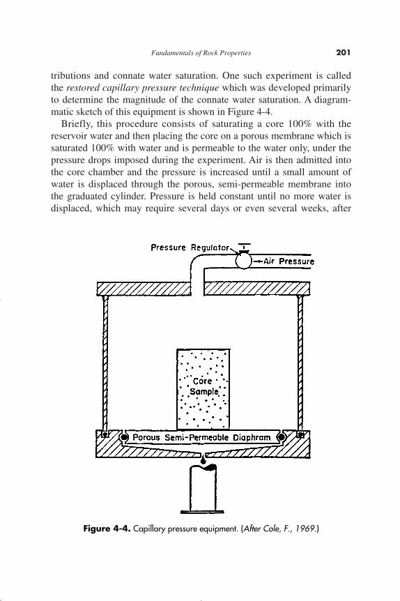
tributions and connate water saturation. One such experiment is calledthe restored capillary pressure technique which was developed primarilyto determine the magnitude of the connate water saturation. A diagram-matic sketch of this equipment is shown in Figure 4-4.
Briefly, this procedure consists of saturating a core 100% with thereservoir water and then placing the core on a porous membrane which issaturated 100% with water and is permeable to the water only, under thepressure drops imposed during the experiment. Air is then admitted intothe core chamber and the pressure is increased until a small amount ofwater is displaced through the porous, semi-permeable membrane intothe graduated cylinder. Pressure is held constant until no more water isdisplaced, which may require several days or even several weeks, after
Fundamentals of Rock Properties 201
Figure 4-4. Capillary pressure equipment. (After Cole, F., 1969.)
Reservoir Eng Hndbk Ch 04a 2001-10-24 09:36 Page 201

which the core is removed from the apparatus and the water saturationdetermined by weighing. The core is then replaced in the apparatus, thepressure is increased, and the procedure is repeated until the water satu-ration is reduced to a minimum.
The data from such an experiment are shown in Figure 4-5. Since thepressure required to displace the wetting phase from the core is exactlyequal to the capillary forces holding the remaining water within the coreafter equilibrium has been reached, the pressure data can be plotted ascapillary pressure data. Two important phenomena can be observed inFigure 4-5. First, there is a finite capillary pressure at 100% water satura-tion that is necessary to force the nonwetting phase into a capillary filledwith the wetting phase. This minimum capillary pressure is known as thedisplacement pressure, pd.
202 Reservoir Engineering Handbook
Figure 4-5. Capillary pressure curve.
Reservoir Eng Hndbk Ch 04a 2001-10-24 09:36 Page 202
If the largest capillary opening is considered as circular with a radius ofr, the pressure needed for forcing the nonwetting fluid out of the core is:
This is the minimum pressure that is required to displace the wettingphase from the largest capillary pore because any capillary of smallerradius will require a higher pressure.
As the wetting phase is displaced, the second phenomenon of anyimmiscible displacement process is encountered, that is, the reaching ofsome finite minimum irreducible saturation. This irreducible water satu-ration is referred to as connate water.
It is possible from the capillary pressure curve to calculate the averagesize of the pores making up a stated fraction of the total pore space. Letpc be the average capillary pressure for the 10% between saturation of 40and 50%. The average capillary radius is obtained from
The above equation may be solved for r providing that the interfacialtension s, and the angle of contact q may be evaluated.
Figure 4-6 is an example of typical oil-water capillary pressure curves.In this case, capillary pressure is plotted versus water saturation for fourrock samples with permeabilities increasing from k1 to k4 . It can be seenthat, for decreases in permeability, there are corresponding increases incapillary pressure at a constant value of water saturation. This is a reflec-tion of the influence of pore size since the smaller diameter pores willinvariably have the lower permeabilities. Also, as would be expected thecapillary pressure for any sample increases with decreasing water satura-tion, another indication of the effect of the radius of curvature of thewater-oil interface.
Capillary Hysteresis
It is generally agreed that the pore spaces of reservoir rocks were orig-inally filled with water, after which oil moved into the reservoir, displac-ing some of the water and reducing the water to some residual saturation.When discovered, the reservoir pore spaces are filled with a connate-water saturation and an oil saturation. All laboratory experiments are
r =2 ( )
pc
s qcos
cP =2 ( )
rs qcos
Fundamentals of Rock Properties 203
Reservoir Eng Hndbk Ch 04a 2001-10-24 09:36 Page 203

designed to duplicate the saturation history of the reservoir. The processof generating the capillary pressure curve by displacing the wettingphase, i.e., water, with the nonwetting phase (such as with gas or oil), iscalled the drainage process.
This drainage process establishes the fluid saturations which are foundwhen the reservoir is discovered. The other principal flow process ofinterest involves reversing the drainage process by displacing the non-wetting phase (such as with oil) with the wetting phase, (e.g., water).This displacing process is termed the imbibition process and the resultingcurve is termed the capillary pressure imbibition curve. The process ofsaturating and desaturating a core with the nonwetting phase is calledcapillary hysteresis. Figure 4-7 shows typical drainage and imbibition
204 Reservoir Engineering Handbook
Figure 4-6. Variation of capillary pressure with permeability.
Reservoir Eng Hndbk Ch 04a 2001-10-24 09:36 Page 204

capillary pressure curves. The two capillary pressure-saturation curvesare not the same.
This difference in the saturating and desaturating of the capillary-pres-sure curves is closely related to the fact that the advancing and recedingcontact angles of fluid interfaces on solids are different. Frequently, innatural crude oil-brine systems, the contact angle or wettability maychange with time. Thus, if a rock sample that has been thoroughlycleaned with volatile solvents is exposed to crude oil for a period of time,it will behave as though it were oil wet. But if it is exposed to brine after
Fundamentals of Rock Properties 205
Figure 4-7. Capillary pressure hysteresis.
Reservoir Eng Hndbk Ch 04a 2001-10-24 09:36 Page 205
cleaning, it will appear water wet. At the present time, one of the greatestunsolved problems in the petroleum industry is that of wettability ofreservoir rock
Another mechanism that has been proposed by McCardell (1955) toaccount for capillary hysteresis is called the ink-bottle effect. This phe-nomenon can be easily observed in a capillary tube having variations inradius along its length. Consider a capillary tube of axial symmetry hav-ing roughly sinusoidal variations in radius. When such a tube has itslower end immersed in water, the water will rise in the tube until thehydrostatic fluid head in the tube becomes equal to the capillary pressure.If then the tube is lifted to a higher level in the water, some water willdrain out, establishing a new equilibrium level in the tube.
When the meniscus is advancing and it approaches a constriction, itjumps through the neck, whereas when receding, it halts without passingthrough the neck. This phenomenon explains why a given capillary pres-sure corresponds to a higher saturation on the drainage curve than on theimbibition curve.
Initial Saturation Distribution in a Reservoir
An important application of the concept of capillary pressures pertainsto the fluid distribution in a reservoir prior to its exploitation. The capil-lary pressure-saturation data can be converted into height-saturation databy arranging Equation 4-29 and solving for the height h above the free-water level.
where pc = capillary pressure, psiaDr = density difference between the wetting and nonwetting
phase, lb/ft3
H = height above the free-water level, ft
Figure 4-8 shows a plot of the water saturation distribution as a func-tion of distance from the free-water level in an oil-water system.
It is essential at this point to introduce and define four important concepts:
• Transition zone• Water-oil contact (WOC)• Gas-oil contact (GOC)• Free water level (FWL)
h =144 pc
D r(4 - 34)
206 Reservoir Engineering Handbook
Reservoir Eng Hndbk Ch 04a 2001-10-24 09:36 Page 206
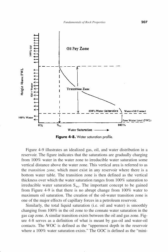
Figure 4-9 illustrates an idealized gas, oil, and water distribution in areservoir. The figure indicates that the saturations are gradually chargingfrom 100% water in the water zone to irreducible water saturation somevertical distance above the water zone. This vertical area is referred to asthe transition zone, which must exist in any reservoir where there is abottom water table. The transition zone is then defined as the verticalthickness over which the water saturation ranges from 100% saturation toirreducible water saturation Swc. The important concept to be gainedfrom Figure 4-9 is that there is no abrupt change from 100% water tomaximum oil saturation. The creation of the oil-water transition zone isone of the major effects of capillary forces in a petroleum reservoir.
Similarly, the total liquid saturation (i.e. oil and water) is smoothlychanging from 100% in the oil zone to the connate water saturation in thegas cap zone. A similar transition exists between the oil and gas zone. Fig-ure 4-8 serves as a definition of what is meant by gas-oil and water-oilcontacts. The WOC is defined as the “uppermost depth in the reservoirwhere a 100% water saturation exists.” The GOC is defined as the “mini-
Fundamentals of Rock Properties 207
Figure 4-8. Water saturation profile.
Reservoir Eng Hndbk Ch 04a 2001-10-24 09:36 Page 207

mum depth at which a 100% liquid, i.e., oil + water, saturation exists inthe reservoir.”
Section A of Figure 4-10 shows a schematic illustration of a core thatis represented by five different pore sizes and completely saturated withwater, i.e., wetting phase. Assume that we subject the core to oil (thenonwetting phase) with increasing pressure until some water is displacedfrom the core, i.e., displacement pressure pd. This water displacementwill occur from the largest pore size. The oil pressure will have toincrease to displace the water in the second largest pore. This sequentialprocess is shown in sections B and C of Figure 4-10.
It should be noted that there is a difference between the free waterlevel (FWL) and the depth at which 100% water saturation exists. From areservoir engineering standpoint, the free water level is defined by zerocapillary pressure. Obviously, if the largest pore is so large that there isno capillary rise in this size pore, then the free water level and 100%water saturation level, i.e., WOC, will be the same. This concept can beexpressed mathematically by the following relationship:
FWL = WOC +144 pd
D r(4 - 35)
208 Reservoir Engineering Handbook
Figure 4-9. Initial saturation profile in a combination-drive reservoir.
Reservoir Eng Hndbk Ch 04a 2001-10-24 09:36 Page 208

where pd = displacement pressure, psiDr = density difference, lb/ft3
FWL = free water level, ftWOC = water-oil contact, ft
Example 4-5
The reservoir capillary pressure-saturation data of the Big Butte Oilreservoir is shown graphically in Figure 4-11. Geophysical log interpreta-tions and core analysis establish the WOC at 5023 ft. The following addi-tional data are available:
• Oil density = 43.5 lb/ft3
• Water density = 64.1 lb/ft3
• Interfacial tension = 50 dynes/cm
Calculate:
• Connate water saturation (Swc)• Depth to FWL• Thickness of the transition zone• Depth to reach 50% water saturation
Fundamentals of Rock Properties 209
Figure 4-10. Relationship between saturation profile and pore-size distribution.
Reservoir Eng Hndbk Ch 04a 2001-10-24 09:36 Page 209

Solution
a. From Figure 4-11, connate-water saturation is 20%.b. Applying Equation 4-35 with a displacement pressure of 1.5 psi gives
c.
d. Pc at 50% water saturation = 3.5 psiaEquivalent height above the FWL = (144) (3.5)/(64.1 - 432.5) = 24.5 ftDepth to 50% water saturation = 5033.5 - 24.5 = 5009 ft
The above example indicates that only oil will flow in the intervalbetween the top of the pay zone and depth of 4991.5 ft. In the transitionzone, i.e., the interval from 4991.5 ft to the WOC, oil production wouldbe accompanied by simultaneous water production.
It should be pointed out that the thickness of the transition zone mayrange from few feet to several hundred feet in some reservoirs. Recallingthe capillary rise equation, i.e., height above FWL,
Thickness of transition zone =144 (6.0 1.5)(64.1 43.5)
= 31.5 ft-
-
FWL = 5023 +(144) (1.5)
(64.1 43.5)= ft
-5033 5.
210 Reservoir Engineering Handbook
Figure 4-11. Capillary pressure saturation data.
Reservoir Eng Hndbk Ch 04a 2001-10-24 09:36 Page 210
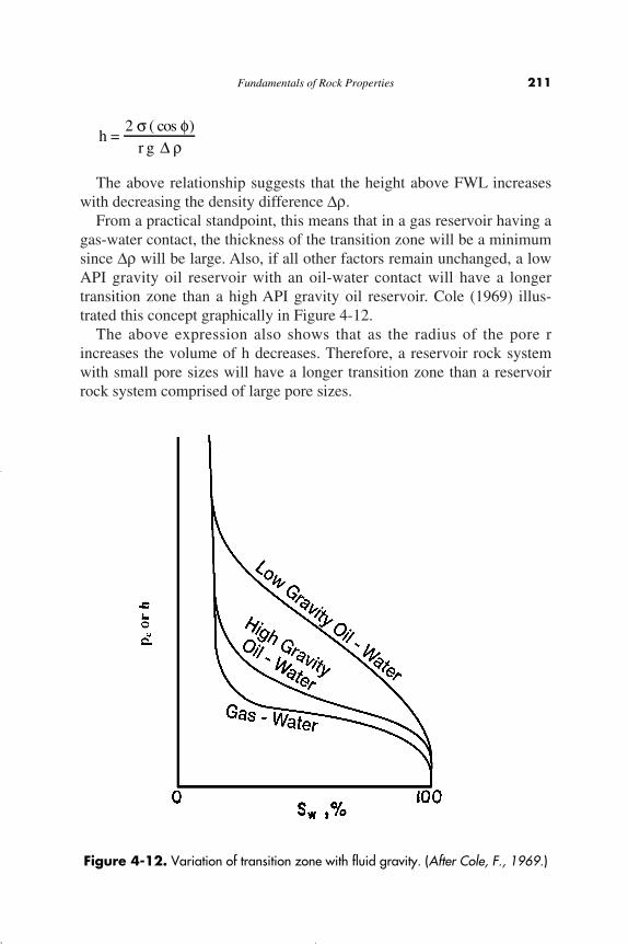
The above relationship suggests that the height above FWL increaseswith decreasing the density difference Dr.
From a practical standpoint, this means that in a gas reservoir having agas-water contact, the thickness of the transition zone will be a minimumsince Dr will be large. Also, if all other factors remain unchanged, a lowAPI gravity oil reservoir with an oil-water contact will have a longertransition zone than a high API gravity oil reservoir. Cole (1969) illus-trated this concept graphically in Figure 4-12.
The above expression also shows that as the radius of the pore rincreases the volume of h decreases. Therefore, a reservoir rock systemwith small pore sizes will have a longer transition zone than a reservoirrock system comprised of large pore sizes.
h =2 s ( cos f)
r g D r
Fundamentals of Rock Properties 211
Figure 4-12. Variation of transition zone with fluid gravity. (After Cole, F., 1969.)
Reservoir Eng Hndbk Ch 04a 2001-10-24 09:36 Page 211

The reservoir pore size can often be related approximately to perme-ability, and where this applies, it can be stated that high permeabilityreservoirs will have shorter transition zones than low permeability reser-voirs as shown graphically in Figure 4-13. As shown by Cole (Figure4-14), a tilted water-oil contact could be caused by a change in perme-ability across the reservoir. It should be emphasized that the factorresponsible for this change in the location of the water-oil contact is actu-ally a change in the size of the pores in the reservoir rock system.
The previous discussion of capillary forces in reservoir rocks hasassumed that the reservoir pore sizes, i.e., permeabilities, are essentiallyuniform. Cole (1969) discussed the effect of reservoir non-uniformity onthe distribution of the fluid saturation through the formation. Figure 4-15shows a hypothetical reservoir rock system that is comprised of sevenlayers. In addition, the seven layers are characterized by only two differ-ent pore sizes, i.e., permeabilities, and corresponding capillary pressure
212 Reservoir Engineering Handbook
Figure 4-13. Variation of transition zone with permeability.
Reservoir Eng Hndbk Ch 04a 2001-10-24 09:36 Page 212

curves as shown in section A of Figure 4-15. The resulting capillary pres-sure curve for the layered reservoir would resemble that shown in sectionB of Figure 4-15. If a well were drilled at the point shown in section B ofFigure 4-15, Layers 1 and 3 would not produce water, while Layer 2,which is above Layer 3, would produce water since it is located in thetransition zone.
Example 4-6
A four-layer oil reservoir is characterized by a set of reservoir capillarypressure-saturation curves as shown in Figure 4-16. The following addi-tional data are also available.
Layer Depth, ft Permeability, md
1 4000–4010 802 4010–4020 1903 4020–4035 704 4035–4060 100
Fundamentals of Rock Properties 213
Low PermeabilityWell No. 1
Medium PermeabilityWell No. 2
High PermeabilityWell No. 3
Tilted
Water-Oil Contact
Water-Oil Contact
pcOR
h
ORh
SwSw
pcpc
OR
h
Figure 4-14. Tilted WOC. (After Cole, F., 1969.)
Reservoir Eng Hndbk Ch 04a 2001-10-24 09:36 Page 213

214 Reservoir Engineering Handbook
Figure 4-15. Effect of permeability on water saturation profile. (After Cole, F., 1969.)
Reservoir Eng Hndbk Ch 04a 2001-10-24 09:36 Page 214

WOC = 4060 ftWater density = 65.2 lb/ft3
Oil density = 55.2 lb/ft3
Calculate and plot water saturation versus depth for this reservoir.
Solution
Step 1. Establish the FWL by determining the displacement pressure pd
for the bottom layer, i.e., Layer 4, and apply Equation 4-37:
• pd = 0.75 psi
Step 2. The top of the bottom layer is located at a depth of 4035 ft whichis 35.8 ft above the FWL. Using that height h of 35.8 ft, calculatethe capillary pressure at the top of the bottom layer.
• cp =h
144=
35.8144
(65.2 55.2) = 2.486 psiÊË
ˆ¯
ÊË
ˆ¯ -D r
FWL = 4060 +(144) (0.75)(65.2 55.2)
= 4070.8 ft-
Fundamentals of Rock Properties 215
Figure 4-16. Variation of pc with k.
Reservoir Eng Hndbk Ch 04a 2001-10-24 09:36 Page 215

• From the capillary pressure-saturation curve designated forLayer 4, read the water saturation that corresponds to a pc of2.486 to give Sw = 0.23.
• Assume different values of water saturations and convert thecorresponding capillary pressures into height above the FWL byapplying Equation 4-34.
Sw pc, psi h, ft Depth = FWL - h
0.23 2.486 35.8 40350.25 2.350 33.84 40370.30 2.150 30.96 40400.40 1.800 25.92 40450.50 1.530 22.03 40490.60 1.340 19.30 40520.70 1.200 17.28 40540.80 1.050 15.12 40560.90 0.900 12.96 4058
Step 3. The top of Layer 3 is located at a distance of 50.8 ft from theFWL (i.e., h = 4070.8 - 4020 = 50.8 ft). Calculate the capillarypressure at the top of the third layer:
• The corresponding water saturation as read from the curve des-ignated for Layer 3 is 0.370.
• Construct the following table for Layer 3.
Sw pc, psi h, ft Depth = FWL - h
0.37 3.53 50.8 40200.40 3.35 48.2 40230.50 2.75 39.6 40310.60 2.50 36.0 4035
• cp =50.8144
(65.2 55.2) = 3.53 psiÊË
ˆ¯ -
h =144 pc
w or r-
216 Reservoir Engineering Handbook
Reservoir Eng Hndbk Ch 04a 2001-10-24 09:36 Page 216
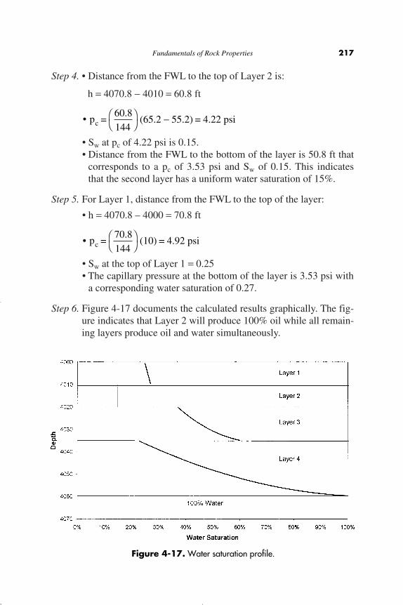
Step 4. • Distance from the FWL to the top of Layer 2 is:
h = 4070.8 - 4010 = 60.8 ft
• Sw at pc of 4.22 psi is 0.15.• Distance from the FWL to the bottom of the layer is 50.8 ft that
corresponds to a pc of 3.53 psi and Sw of 0.15. This indicatesthat the second layer has a uniform water saturation of 15%.
Step 5. For Layer 1, distance from the FWL to the top of the layer:
• h = 4070.8 – 4000 = 70.8 ft
• Sw at the top of Layer 1 = 0.25• The capillary pressure at the bottom of the layer is 3.53 psi with
a corresponding water saturation of 0.27.
Step 6. Figure 4-17 documents the calculated results graphically. The fig-ure indicates that Layer 2 will produce 100% oil while all remain-ing layers produce oil and water simultaneously.
• cp =70.8144
(10) = 4.92 psiÊË
ˆ¯
cp =60.8144
(65.2 55.2) = 4.22 psi• ÊË
ˆ¯ -
Fundamentals of Rock Properties 217
Figure 4-17. Water saturation profile.
Reservoir Eng Hndbk Ch 04a 2001-10-24 09:36 Page 217

Leverett J-Function
Capillary pressure data are obtained on small core samples that repre-sent an extremely small part of the reservoir and, therefore, it is neces-sary to combine all capillary data to classify a particular reservoir. Thefact that the capillary pressure-saturation curves of nearly all naturallyporous materials have many features in common has led to attempts todevise some general equation describing all such curves. Leverett (1941)approached the problem from the standpoint of dimensional analysis.
Realizing that capillary pressure should depend on the porosity, inter-facial tension, and mean pore radius, Leverett defined the dimensionlessfunction of saturation, which he called the J-function, as
where J(Sw) = Leverett J-functionpc = capillary pressure, psis = interfacial tension, dynes/cmk = permeability, mdf = fractional porosity
In doing so, Leverett interpreted the ratio of permeability, k, to porosi-ty, f, as being proportional to the square of a mean pore radius.
The J-function was originally proposed as a means of converting allcapillary-pressure data to a universal curve. There are significant differ-ences in correlation of the J-function with water saturation from forma-tion to formation, so that no universal curve can be obtained. For thesame formation, however, this dimensionless capillary-pressure functionserves quite well in many cases to remove discrepancies in the pc versusSw curves and reduce them to a common curve. This is shown for variousunconsolidated sands in Figure 4-18.
Example 4-7
A laboratory capillary pressure test was conducted on a core sampletaken from the Nameless Field. The core has a porosity and permeabilityof 16% and 80 md, respectively. The capillary pressure-saturation dataare given as follows:
J (S ) = 0.21645p k
wc
s f(4 - 36)
218 Reservoir Engineering Handbook
Reservoir Eng Hndbk Ch 04a 2001-10-24 09:36 Page 218

Sw pc, psi
1.0 0.500.8 0.600.6 0.750.4 1.050.2 1.75
Fundamentals of Rock Properties 219
Figure 4-18. The Leverett J-function for unconsolidated sands. (After Leverett, 1941.)
Reservoir Eng Hndbk Ch 04a 2001-10-24 09:36 Page 219
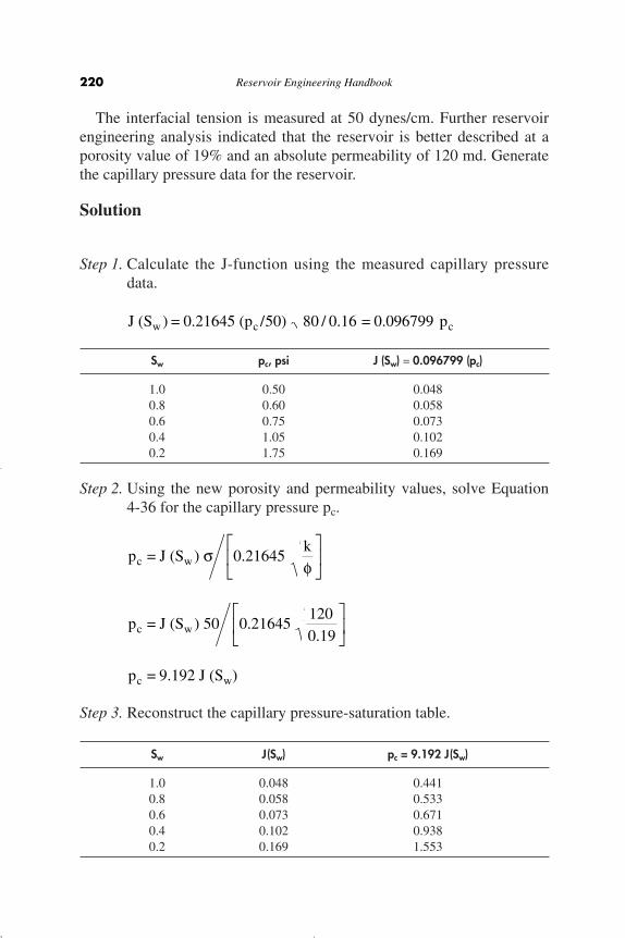
The interfacial tension is measured at 50 dynes/cm. Further reservoirengineering analysis indicated that the reservoir is better described at aporosity value of 19% and an absolute permeability of 120 md. Generatethe capillary pressure data for the reservoir.
Solution
Step 1. Calculate the J-function using the measured capillary pressuredata.
Sw pc, psi J (Sw) = 0.096799 (pc)
1.0 0.50 0.0480.8 0.60 0.0580.6 0.75 0.0730.4 1.05 0.1020.2 1.75 0.169
Step 2. Using the new porosity and permeability values, solve Equation4-36 for the capillary pressure pc.
Step 3. Reconstruct the capillary pressure-saturation table.
Sw J(Sw) pc = 9.192 J(Sw)
1.0 0.048 0.4410.8 0.058 0.5330.6 0.073 0.6710.4 0.102 0.9380.2 0.169 1.553
p = J (S ) 0.21645k
p = J (S ) 50 0.21645
p = 9.192 J (S )
c w
c w
c w
sf
È
ÎÍ
˘
˚˙
È
ÎÍ
˘
˚˙
1200 19.
J (S ) = 0.21645 (p /50) 80 / 0.16 = 0.096799 pw c c
220 Reservoir Engineering Handbook
Reservoir Eng Hndbk Ch 04a 2001-10-24 09:36 Page 220
Converting Laboratory Capillary Pressure Data
For experimental convenience, it is common in the laboratory determi-nation of capillary pressure to use air-mercury or air-brine systems,rather than the actual water-oil system characteristic of the reservoir.Since the laboratory fluid system does not have the same surface tensionas the reservoir system, it becomes necessary to convert laboratory capil-lary pressure to reservoir capillary pressure. By assuming that the Lev-erett J-function is a property of rock and does not change from the labo-ratory to the reservoir, we can calculate reservoir capillary pressure asshow below.
Even after the laboratory capillary pressure has been corrected for sur-face tension, it may be necessary to make further corrections for perme-ability and porosity. The reason for this is that the core sample that wasused in performing the laboratory capillary pressure test may not be rep-resentative of the average reservoir permeability and porosity. If weassume that the J-function will be invariant for a given rock type over arange of porosity and permeability values, then the reservoir capillarypressure can be expressed as
where (pc)res = reservoir capillary pressuresres = reservoir surface or interfacial tensionkres = reservoir permeabilityfres = reservoir porosity
(pc)lab = laboratory measured capillary pressurefcore = core porositykcore = core permeability
PERMEABILITY
Permeability is a property of the porous medium that measures thecapacity and ability of the formation to transmit fluids. The rock perme-ability, k, is a very important rock property because it controls the direc-
( ) ( )p = p ( k ) / ( k )c res c labres
labres core core res
ss
f f (4 - 37)
( ) ( )p pc res c labres
lab= s
s
Fundamentals of Rock Properties 221
Reservoir Eng Hndbk Ch 04a 2001-10-24 09:36 Page 221
tional movement and the flow rate of the reservoir fluids in the forma-tion. This rock characterization was first defined mathematically byHenry Darcy in 1856. In fact, the equation that defines permeability interms of measurable quantities is called Darcy’s Law.
Darcy developed a fluid flow equation that has since become one ofthe standard mathematical tools of the petroleum engineer. If a horizontallinear flow of an incompressible fluid is established through a core sam-ple of length L and a cross-section of area A, then the governing fluidflow equation is defined as
where n = apparent fluid flowing velocity, cm/seck = proportionality constant, or permeability, Darcysm = viscosity of the flowing fluid, cp
dp/dL = pressure drop per unit length, atm/cm
The velocity, n, in Equation 4-38 is not the actual velocity of the flowingfluid but is the apparent velocity determined by dividing the flow rate bythe cross-sectional area across which fluid is flowing. Substituting the rela-tionship, q/A, in place of n in Equation 4-38 and solving for q results in
where q = flow rate through the porous medium, cm3/secA = cross-sectional area across which flow occurs, cm2
With a flow rate of one cubic centimeter per second across a cross-sectional area of one square centimeter with a fluid of one centipoise vis-cosity and a pressure gradient at one atmosphere per centimeter oflength, it is obvious that k is unity. For the units described above, k hasbeen arbitrarily assigned a unit called Darcy in honor of the man respon-sible for the development of the theory of flow through porous media.Thus, when all other parts of Equation 4-39 have values of unity, k has avalue of one Darcy.
One Darcy is a relatively high permeability as the permeabilities ofmost reservoir rocks are less than one Darcy. In order to avoid the use of
q =kA dp
dL-
m(4 - 39)
nm
=k dp
dL- (4 - 38)
222 Reservoir Engineering Handbook
Reservoir Eng Hndbk Ch 04a 2001-10-24 09:36 Page 222
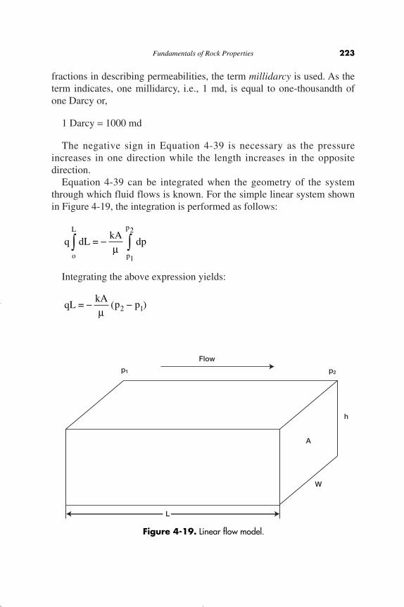
fractions in describing permeabilities, the term millidarcy is used. As theterm indicates, one millidarcy, i.e., 1 md, is equal to one-thousandth ofone Darcy or,
1 Darcy = 1000 md
The negative sign in Equation 4-39 is necessary as the pressureincreases in one direction while the length increases in the oppositedirection.
Equation 4-39 can be integrated when the geometry of the systemthrough which fluid flows is known. For the simple linear system shownin Figure 4-19, the integration is performed as follows:
Integrating the above expression yields:
qL =kA
(p p )2 1- -m
q dL =kA
dpo
L
1p
2p
Ú Ú-m
Fundamentals of Rock Properties 223
Flow
p1 p2
h
A
W
L
Figure 4-19. Linear flow model.
Reservoir Eng Hndbk Ch 04a 2001-10-24 09:37 Page 223

It should be pointed out that the volumetric flow rate, q, is constant forliquids because the density does not change significantly with pressure.
Since p1 is greater than p2, the pressure terms can be rearranged, whichwill eliminate the negative term in the equation. The resulting equation is:
Equation 4-40 is the conventional linear flow equation used in fluidflow calculations.
Standard laboratory analysis procedures will generally provide reliabledata on permeability of core samples. If the rock is not homogeneous, thewhole core analysis technique will probably yield more accurate resultsthan the analysis of core plugs (small pieces cut from the core). Proceduresthat have been used for improving the accuracy of the permeability deter-mination include cutting the core with an oil-base mud, employing a pres-sure-core barrel, and conducting the permeability tests with reservoir oil.
Permeability is reduced by overburden pressure, and this factor shouldbe considered in estimating permeability of the reservoir rock in deepwells because permeability is an isotropic property of porous rock insome defined regions of the system, that is, it is directional. Routine coreanalysis is generally concerned with plug samples drilled parallel to bed-ding planes and, hence, parallel to direction of flow in the reservoir.These yield horizontal permeabilities (kh).
The measured permeability on plugs that are drilled perpendicular tobedding planes are referred to as vertical permeability (kv). Figure 4-20shows a schematic illustration of the concept of the core plug and theassociated permeability.
As shown in Figure 4-20, there are several factors that must be consid-ered as possible sources of error in determining reservoir permeability.These factors are:
1. Core sample may not be representative of the reservoir rock becauseof reservoir heterogeneity.
2. Core recovery may be incomplete.3. Permeability of the core may be altered when it is cut, or when it is
cleaned and dried in preparation for analysis. This problem is likely tooccur when the rock contains reactive clays.
4. Sampling process may be biased. There is a temptation to select thebest parts of the core for analysis.
q =kA (p p )
L1 2-
m(4 - 40)
224 Reservoir Engineering Handbook
Reservoir Eng Hndbk Ch 04a 2001-10-24 09:37 Page 224
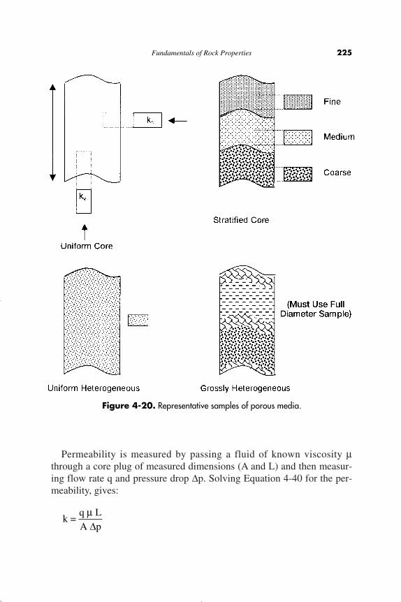
Permeability is measured by passing a fluid of known viscosity mthrough a core plug of measured dimensions (A and L) and then measur-ing flow rate q and pressure drop Dp. Solving Equation 4-40 for the per-meability, gives:
k =q LA p
mD
Fundamentals of Rock Properties 225
Figure 4-20. Representative samples of porous media.
Reservoir Eng Hndbk Ch 04a 2001-10-24 09:37 Page 225
where L = length of core, cmA = cross-sectional area, cm2
The following conditions must exist during the measurement of per-meability:
• Laminar (viscous) flow• No reaction between fluid and rock• Only single phase present at 100% pore space saturation
This measured permeability at 100% saturation of a single phase iscalled the absolute permeability of the rock.
Example 4-8
A brine is used to measure the absolute permeability of a core plug.The rock sample is 4 cm long and 3 cm2 in cross section. The brine has aviscosity of 1.0 cp and is flowing a constant rate of 0.5 cm3/sec under a2.0 atm pressure differential. Calculate the absolute permeability.
Solution
Applying Darcy’s equation, i.e., Equation 4-40, gives:
Example 4-9
Rework the above example assuming that an oil of 2.0 cp is used tomeasure the permeability. Under the same differential pressure, the flowrate is 0.25 cm3/sec.
0.5 =(k) (3) (2)
(1) (4)
k = 0.333 Darcys
226 Reservoir Engineering Handbook
Reservoir Eng Hndbk Ch 04a 2001-10-24 09:37 Page 226

Solution
Applying Darcy’s equation yields:
Dry gas is usually used (air, N2, He) in permeability determinationbecause of its convenience, availability, and to minimize fluid-rockreaction.
The measurement of the permeability should be restricted to the low(laminar/viscous) flow rate region, where the pressure remains propor-tional to flow rate within the experimental error. For high flow rates,Darcy’s equation as expressed by Equation 4-40 is inappropriate todescribe the relationship of flow rate and pressure drop.
In using dry gas in measuring the permeability, the gas volumetricflow rate q varies with pressure because the gas is a highly compressiblefluid. Therefore, the value of q at the average pressure in the core mustbe used in Equation 4-40. Assuming the used gases follow the ideal gasbehavior (at low pressures), the following relationships apply:
p1V1 = p2 V2 = pmVm
In terms of the flow rate q, the above equation can be equivalentlyexpressed as:
p1 q1 = p2 q2 = pm qm (4-41)
with the mean pressure pm expressed as:
where p1, p2, pm = inlet, outlet, and mean pressures, respectively, atmV1, V2, Vm = inlet, outlet, and mean gas volume, respectively, cm3
q1, q2, qm = inlet, outlet, and mean gas flow rate, respectively,cm3/sec
m1 2p =
p p
2
+
0.25 =(k) (3) (2)
(2) (4)
k = 0.333 Darcys
Fundamentals of Rock Properties 227
Reservoir Eng Hndbk Ch 04a 2001-10-24 09:37 Page 227
The gas flow rate is usually measured at base (atmospheric) pressure pb
and, therefore, the term Qgsc is introduced into Equation 4-41 to produce:
Qgsc pb = qm pm
where Qgsc = gas flow rate at standard conditions, cm3/secpb = base pressure (atmospheric pressure), atm
Substituting Darcy’s Law in the above expression gives
or
where k = absolute permeability, Darcysmg = gas viscosity, cppb = base pressure, atmp1 = inlet (upstream) pressure, atmp2 = outlet (downstream) pressure, atmL = length of the core, cmA = cross-sectional area, cm2
Qgsc = gas flow rate at standard conditions, cm3/sec
The Klinkenberg Effect
Klinkenberg (1941) discovered that permeability measurements madewith air as the flowing fluid showed different results from permeabilitymeasurements made with a liquid as the flowing fluid. The permeabilityof a core sample measured by flowing air is always greater than the per-meability obtained when a liquid is the flowing fluid. Klinkenberg postu-lated, on the basis of his laboratory experiments, that liquids had a zerovelocity at the sand grain surface, while gases exhibited some finitevelocity at the sand grain surface. In other words, the gases exhibitedslippage at the sand grain surface. This slippage resulted in a higher flowrate for the gas at a given pressure differential. Klinkenberg also foundthat for a given porous medium as the mean pressure increased the calcu-lated permeability decreased.
gsc12
22
g b
Q =k A (p p )
2 L p-
m(4 - 42)
gsc b1 2
g
1 2Q p =k A (p p )
L
p + p
2
- ÊË
ˆ¯m
228 Reservoir Engineering Handbook
Reservoir Eng Hndbk Ch 04a 2001-10-24 09:37 Page 228

Fundamentals of Rock Properties 229
Mean pressure is defined as upstream flowing plus downstream flow-ing pressure divided by two, [pm = (p1 + p2)/2]. If a plot of measured per-meability versus 1/pm were extrapolated to the point where 1/pm = 0, inother words, where pm = infinity, this permeability would be approxi-mately equal to the liquid permeability. A graph of this nature is shown inFigure 4-21. The absolute permeability is determined by extrapolation asshown in Figure 4-21.
The magnitude of the Klinkenberg effect varies with the core perme-ability and the type of the gas used in the experiment as shown in Figures4-22 and 4-23. The resulting straight-line relationship can be expressed as
where kg = measured gas permeabilitypm = mean pressurekL = equivalent liquid permeability, i.e., absolute permeability, kc = slope of the line
g Lm
k = k + c1
p
È
ÎÍ
˘
˚˙ (4 - 43)
Figure 4-21. The Klinkenberg effect in gas permeability measurements.
Reservoir Eng Hndbk Ch 04b 2001-10-24 09:46 Page 229

Klinkenberg suggested that the slope Ac @ is a function of the follow-ing factors:
• Absolute permeability k, i.e., permeability of medium to a single phasecompletely filling the pores of the medium kL.
• Type of the gas used in measuring the permeability, e.g., air.• Average radius of the rock capillaries.
Klinkenberg expressed the slope c by the following relationship:
c = bkL (4-44)
where kL = equivalent liquid permeability, i.e., absolute permeability, kb = constant which depends on the size of the pore openings
and is inversely proportional to radius of capillaries.
230 Reservoir Engineering Handbook
Figure 4-22. Effect of permeability on the magnitude of the Klinkenberg effect.(After Cole, F., 1969.)
Reservoir Eng Hndbk Ch 04b 2001-10-24 09:46 Page 230

Combining Equation 4-44 with 4-43 gives:
where kg is the gas permeability as measured at the average pressure pm.
Jones (1972) studied the gas slip phenomena for a group of cores forwhich porosity, liquid permeability kL (absolute permeability), and airpermeability were determined. He correlated the parameter b with theliquid permeability by the following expression:
b = 6.9 kL-0.36 (4-46)
The usual measurement of permeability is made with air at mean pres-sure just above atmospheric pressure (1 atm). To evaluate the slip phe-nomenon and the Klinkenberg effect, it is necessary to at least measurethe gas permeability at two mean-pressure levels. In the absence of suchdata, Equations 4-45 and 4-46 can be combined and arranged to give:
6.9 kL0.64 + pm kL - pm kg = 0 (4-47)
g L Lm
k = k + b k1
p( )
È
ÎÍ
˘
˚˙ (4 - 45)
Fundamentals of Rock Properties 231
Figure 4-23. Effect of gas pressure on measured permeability for various gases.(After Calhoun, J., 1976.)
Reservoir Eng Hndbk Ch 04b 2001-10-24 09:46 Page 231
where pm = mean pressure, psikg = air permeability at pm, psikL = absolute permeability (k), md
Equation 4-47 can be used to calculate the absolute permeability whenonly one gas permeability measurement (kg) of a core sample is made atpm. This nonlinear equation can be solved iteratively by using the New-ton-Raphson iterative methods. The proposed solution method can beconveniently written as
where ki = initial guess of the absolute permeability, mdki+1 = new permeability value to be used for the next iteration
i = iteration level f(ki) = Equation 4-47 as evaluated by using the assumed value of ki.f¢(ki) = first-derivative of Equation 4-47 as evaluated at ki
The first derivative of Equation 4-47 with respect to ki is:
f¢ (ki) = 4.416 ki-0.36 + pm (4-48)
The iterative procedure is repeated until convergence is achieved whenf(ki) approaches zero or when no changes in the calculated values of ki
are observed.
Example 4-10
The permeability of a core plug is measured by air. Only one measure-ment is made at a mean pressure of 2.152 psi. The air permeability is46.6 md. Estimate the absolute permeability of the core sample. Comparethe result with the actual absolute permeability of 23.66 md.
Solution
Step 1. Substitute the given values of pm and kg into Equations 4-47 and4-48, to give:
f (ki) = 6.9 ki0.64 + 2.152 ki - (2.152) (46.6) f¢ (ki) = 4.416 ki
-0.36
+ 2.152
i + 1 ii
ik = k
f (k )f (k )
-¢
232 Reservoir Engineering Handbook
Reservoir Eng Hndbk Ch 04b 2001-10-24 09:46 Page 232

Step 2. Assume ki = 30 and apply the Newton-Raphson method to findthe required solution as shown below.
i ki f (ki) f¢(ki) k i + 1
1 30.000 25.12 3.45 22.7192 22.719 -0.466 3.29 22.8613 22.861 0.414 3.29 22.848
After three iterations, the Newton-Raphson method converges to anabsolute value for the permeability of 22.848 md.
Equation 4-39 can be expanded to describe flow in any porous medi-um where the geometry of the system is not too complex to integrate. Forexample, the flow into a well bore is not linear, but is more often radial.Figure 4-24 illustrates the type of flow that is typical of that occurring inthe vicinity of a producing well. For a radial flow, Darcy’s equation in adifferential form can be written as:
Fundamentals of Rock Properties 233
Figure 4-24. Radial flow model.
Reservoir Eng Hndbk Ch 04b 2001-10-24 09:46 Page 233
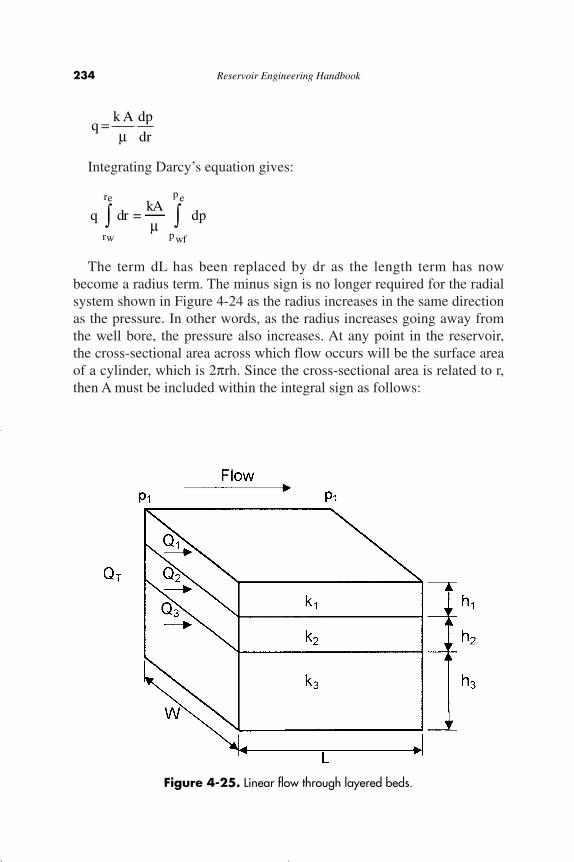
Integrating Darcy’s equation gives:
The term dL has been replaced by dr as the length term has nowbecome a radius term. The minus sign is no longer required for the radialsystem shown in Figure 4-24 as the radius increases in the same directionas the pressure. In other words, as the radius increases going away fromthe well bore, the pressure also increases. At any point in the reservoir,the cross-sectional area across which flow occurs will be the surface areaof a cylinder, which is 2prh. Since the cross-sectional area is related to r,then A must be included within the integral sign as follows:
q
wr
er
Ú dr =kA
mwfp
ep
Ú dp
qk A dp
dr=
m
234 Reservoir Engineering Handbook
Figure 4-25. Linear flow through layered beds.
Reservoir Eng Hndbk Ch 04b 2001-10-24 09:46 Page 234
rearranging
and integrating
Solving for the flow rate, q, results in:
The above equation assumes that the reservoir is homogeneous and iscompletely saturated with a single liquid phase (appropriate modifica-tions will be discussed in later sections to account for the presence ofother fluids), where:
q = flow rate, reservoir cm3/seck = absolute permeability, Darcyh = thickness, cmre = drainage radius, cmrw = well bore radius, cmpe = pressure at drainage radius, atm
pwf = bottom-hole flowing pressurem = viscosity, cp
Averaging Absolute Permeabilities
The most difficult reservoir properties to determine usually are thelevel and distribution of the absolute permeability throughout the reser-voir. They are more variable than porosity and more difficult to measure.Yet an adequate knowledge of permeability distribution is critical to the
q =2 kh (p p )
r /re wf
e w
pm
-ln ( )
(4 - 49)
q2 h
( r r ) =k
(p p )e w e wfp mln ln- -
q2 h
drr
=k
dp
wr
er
wfp
ep
p mÚ Ú
qdr
2 rh=
kdp
wr
er
wfp
ep
Ú Úp m
Fundamentals of Rock Properties 235
Reservoir Eng Hndbk Ch 04b 2001-10-24 09:46 Page 235

prediction of reservoir depletion by any recovery process. It is rare toencounter a homogeneous reservoir in actual practice. In many cases, thereservoir contains distinct layers, blocks, or concentric rings of varyingpermeabilities. Also, because smaller-scale heterogeneities always exist,core permeabilities must be averaged to represent the flow characteristicsof the entire reservoir or individual reservoir layers (units). The properway of averaging the permeability data depends on how permeabilitieswere distributed as the rock was deposited.
There are three simple permeability-averaging techniques that arecommonly used to determine an appropriate average permeability to rep-resent an equivalent homogeneous system. These are:
• Weighted-average permeability• Harmonic-average permeability• Geometric-average permeability
Weighted-Average Permeability
This averaging method is used to determine the average permeabilityof layered-parallel beds with different permeabilities. Consider the casewhere the flow system is comprised of three parallel layers that are sepa-rated from one another by thin impermeable barriers, i.e., no cross flow,as shown in Figure 4-25. All the layers have the same width w with across-sectional area of A.
The flow from each layer can be calculated by applying Darcy’s equa-tion in a linear form as expressed by Equation 4-40, to give:
Layer 1
Layer 2
Layer 3
qk w h p
L33 3= D
m
22 2q = k w h p
LD
m
11 1q = k w h p
LD
m
236 Reservoir Engineering Handbook
Reservoir Eng Hndbk Ch 04b 2001-10-24 09:46 Page 236
The total flow rate from the entire system is expressed as
where qt = total flow ratekavg = average permeability for the entire model
w = width of the formationDp = p1 B p2
ht = total thickness
The total flow rate qt is equal to the sum of the flow rates through eachlayer or:
qt = q1 + q2 + q3
Combining the above expressions gives:
or
The average absolute permeability for a parallel-layered system can beexpressed in the following form:
Equation 4-50 is commonly used to determine the average permeabili-ty of a reservoir from core analysis data.
avgj 1
n
j j
jj
nk =
k h
h
=
=
Â
Â1
(4 - 50)
avg t 2 2
avg1 1 2 2 3 3
t
k h = k h + k h + k h
k = k h + k h + k hh
1 1 3 3
avg t 1 1 2 2 3 3k w h p
L= k w h p
L+ k w h p
L+ k w h p
L
D D D Dm m m m
qk w h p
Ltavg t=
Dm
Fundamentals of Rock Properties 237
Reservoir Eng Hndbk Ch 04b 2001-10-24 09:46 Page 237
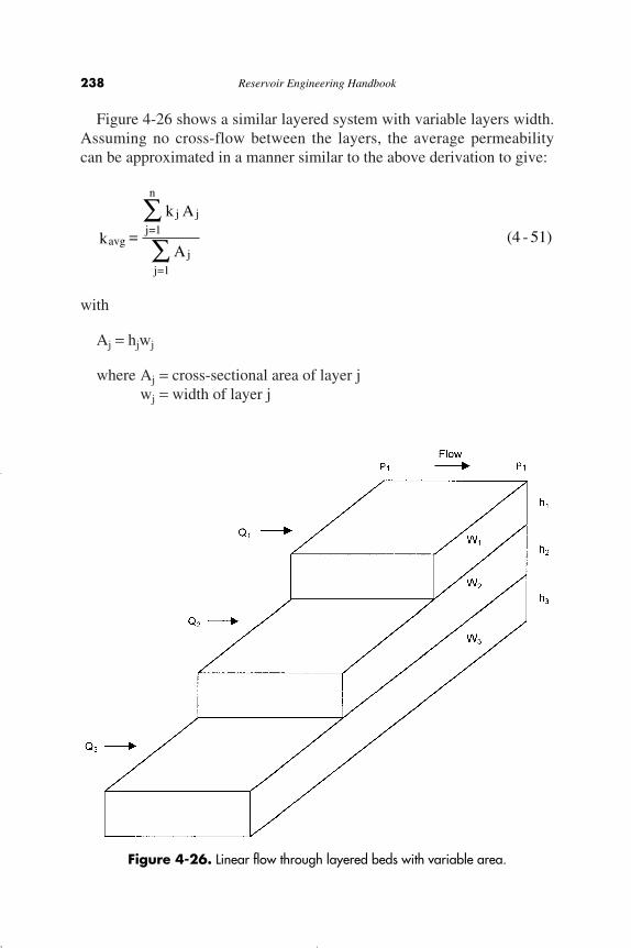
Figure 4-26 shows a similar layered system with variable layers width.Assuming no cross-flow between the layers, the average permeabilitycan be approximated in a manner similar to the above derivation to give:
with
Aj = hjwj
where Aj = cross-sectional area of layer jwj = width of layer j
avgj=1
n
j j
j=1j
k =
k A
A
ÂÂ
(4 - 51)
238 Reservoir Engineering Handbook
Figure 4-26. Linear flow through layered beds with variable area.
Reservoir Eng Hndbk Ch 04b 2001-10-24 09:46 Page 238

Example 4-11
Given the following permeability data from a core analysis report, cal-culate the average permeability of the reservoir.
Depth, ft Permeability, md
3998-02 2004002-04 1304004-06 1704006-08 1804008-10 140
Solution
hi, ft ki hiki
4 200 8002 130 2602 170 3402 180 3602 140 280
ht = 12 ∑ hiki = 2040
Harmonic-Average Permeability
Permeability variations can occur laterally in a reservoir as well as inthe vicinity of a well bore. Consider Figure 4-27 which shows an illustra-tion of fluid flow through a series combination of beds with different per-meabilities.
For a steady-state flow, the flow rate is constant and the total pressuredrop Dp is equal to the sum of the pressure drops across each bed, or
Dp = Dp1 + Dp2 + Dp3
Substituting for the pressure drop by applying Darcy’s equation, i.e.,Equation 4-40, gives:
avgk =204012
= 170 md
Fundamentals of Rock Properties 239
Reservoir Eng Hndbk Ch 04b 2001-10-24 09:46 Page 239
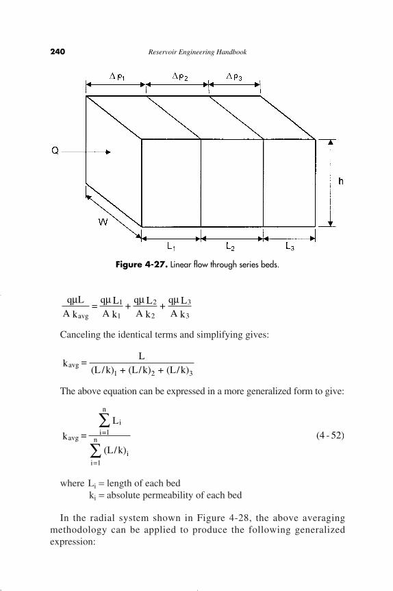
Canceling the identical terms and simplifying gives:
The above equation can be expressed in a more generalized form to give:
where Li = length of each bedki = absolute permeability of each bed
In the radial system shown in Figure 4-28, the above averagingmethodology can be applied to produce the following generalizedexpression:
avgi=1
n
i
i=1
n
i
k =
L
(L/k)
Â
Â(4 - 52)
avg1 2 3
k =L
(L /k) + (L/k) + (L/k)
q LA k
=q LA k
+q LA k
+q LA kavg
1
1
2
2
3
3
m m m m
240 Reservoir Engineering Handbook
Figure 4-27. Linear flow through series beds.
Reservoir Eng Hndbk Ch 04b 2001-10-24 09:46 Page 240
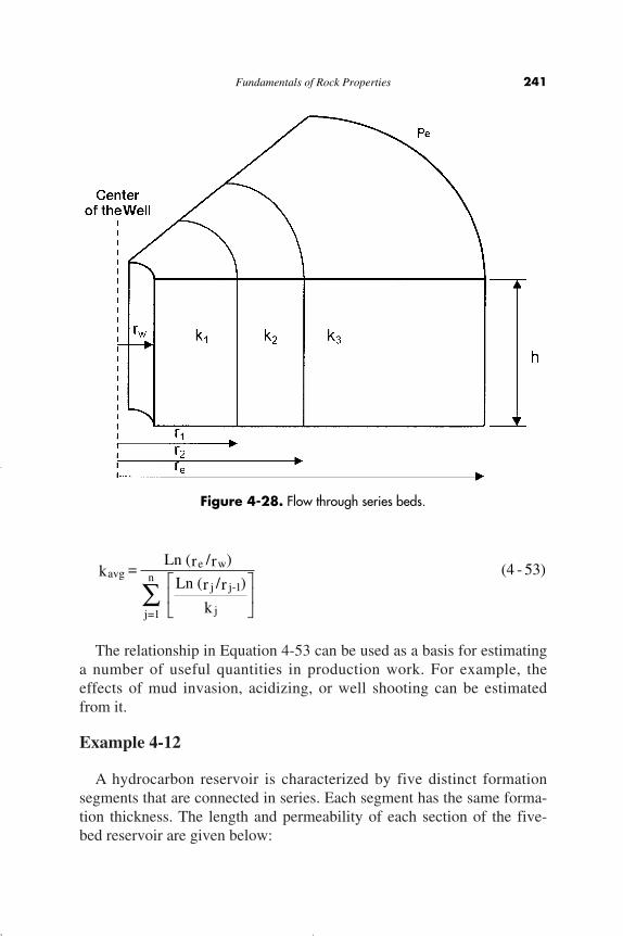
The relationship in Equation 4-53 can be used as a basis for estimatinga number of useful quantities in production work. For example, theeffects of mud invasion, acidizing, or well shooting can be estimatedfrom it.
Example 4-12
A hydrocarbon reservoir is characterized by five distinct formationsegments that are connected in series. Each segment has the same forma-tion thickness. The length and permeability of each section of the five-bed reservoir are given below:
avge w
j=1
nj j-1
j
k =(r /r )
(r /r )
k
Ln
Ln È
ÎÍ
˘
˚˙
(4 - 53)
Fundamentals of Rock Properties 241
Figure 4-28. Flow through series beds.
Reservoir Eng Hndbk Ch 04b 2001-10-24 09:46 Page 241

Length, ft Permeability, md
150 80200 50300 30500 20200 10
Calculate the average permeability of the reservoir by assuming:
a. Linear flow systemb. Radial flow system
Solution
For a linear system:
Li, ft ki Li/ki
150 80 1.8750200 50 4.0000300 30 10.000500 20 25.000200 10 20.000
1350 S Li/ki = 60.875
Using Equation 4-52 gives:
For a radial system:
The solution of the radial system can be conveniently expressed in thefollowing tabulated form. The solution is based on Equation 4-53 andassuming a wellbore radius of 0.25 ft:
Segment ri, ft ln(ri/riB1) ki [ln(ri/riB1)]/ki
well bore 0.25 — — —1 150 6.397 80 0.0802 350 0.847 50 0.0173 650 0.619 30 10.0214 1150 0.571 20 0.0295 1350 0.160 10 0.016
0.163
avgk =1350
60.875= 22.18 md
242 Reservoir Engineering Handbook
Reservoir Eng Hndbk Ch 04b 2001-10-24 09:46 Page 242

From Equation 4-53,
Geometric-Average Permeability
Warren and Price (1961) illustrated experimentally that the most proba-ble behavior of a heterogeneous formation approaches that of a uniformsystem having a permeability that is equal to the geometric average. Thegeometric average is defined mathematically by the following relationship:
where ki = permeability of core sample ihi = thickness of core sample in = total number of samples
If the thicknesses (hi) of all core samples are the same, Equation 4-57can be simplified as follows:
Example 4-13
Given the following core data, calculate the geometric average perme-ability:
Sample hi, ft ki, md
1 1.0 102 1.0 303 0.5 1004 1.5 405 2.0 806 1.5 707 1.0 158 1.0 509 1.5 35
10 0.5 20
k = k k k kavg nn( )1 2 3
1
K (4 - 55)
avgi=1
n
i i
i=1
n
i
k =
h k
h
exp
( ln ( ))Â
Â
È
Î
ÍÍÍÍÍ
˘
˚
˙˙˙˙˙
(4 - 54)
avgk =l (1350 /0.25)
0.163= 52.72 md
n
Fundamentals of Rock Properties 243
Reservoir Eng Hndbk Ch 04b 2001-10-24 09:46 Page 243
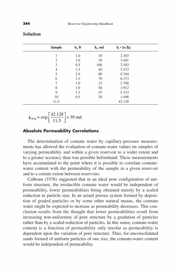
Solution
Sample hi, ft ki, md hi * Ln (ki)
1 1.0 10 2.3032 1.0 30 3.4013 0.5 100 2.3034 1.5 40 5.5335 2.0 80 8.7646 1.5 70 6.3737 1.0 15 2.7088 1.0 50 3.9129 1.5 35 5.33310 0.5 20 1.498
11.5 42.128
Absolute Permeability Correlations
The determination of connate water by capillary-pressure measure-ments has allowed the evaluation of connate-water values on samples ofvarying permeability and within a given reservoir to a wider extent andto a greater accuracy than was possible beforehand. These measurementshave accumulated to the point where it is possible to correlate connate-water content with the permeability of the sample in a given reservoirand to a certain extent between reservoirs.
Calhoun (1976) suggested that in an ideal pore configuration of uni-form structure, the irreducible connate water would be independent ofpermeability, lower permeabilities being obtained merely by a scaledreduction in particle size. In an actual porous system formed by deposi-tion of graded particles or by some other natural means, the connatewater might be expected to increase as permeability decreases. This con-clusion results from the thought that lower permeabilities result fromincreasing non-uniformity of pore structure by a gradation of particlesrather than by a scaled reduction of particles. In this sense, connate-watercontent is a function of permeability only insofar as permeability isdependent upon the variation of pore structure. Thus, for unconsolidatedsands formed of uniform particles of one size, the connate-water contentwould be independent of permeability.
avgk =42.12811.5
= 39 mdexp ÈÎÍ
˘˚
244 Reservoir Engineering Handbook
Reservoir Eng Hndbk Ch 04b 2001-10-24 09:46 Page 244
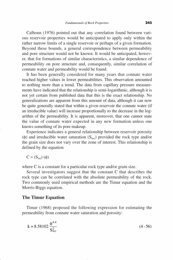
Calhoun (1976) pointed out that any correlation found between vari-ous reservoir properties would be anticipated to apply only within therather narrow limits of a single reservoir or perhaps of a given formation.Beyond these bounds, a general correspondence between permeabilityand pore structure would not be known. It would be anticipated, howev-er, that for formations of similar characteristics, a similar dependence ofpermeability on pore structure and, consequently, similar correlation ofconnate water and permeability would be found.
It has been generally considered for many years that connate waterreached higher values in lower permeabilities. This observation amountedto nothing more than a trend. The data from capillary pressure measure-ments have indicated that the relationship is semi-logarithmic, although it isnot yet certain from published data that this is the exact relationship. Nogeneralizations are apparent from this amount of data, although it can nowbe quite generally stated that within a given reservoir the connate water (ifan irreducible value) will increase proportionally to the decrease in the log-arithm of the permeability. It is apparent, moreover, that one cannot statethe value of connate water expected in any new formation unless oneknows something of its pore makeup.
Experience indicates a general relationship between reservoir porosity(f) and irreducible water saturation (Swc) provided the rock type and/orthe grain size does not vary over the zone of interest. This relationship isdefined by the equation
C = (Swi) (f)
where C is a constant for a particular rock type and/or grain size.Several investigators suggest that the constant C that describes the
rock type can be correlated with the absolute permeability of the rock.Two commonly used empirical methods are the Timur equation and theMorris-Biggs equation.
The Timur Equation
Timur (1968) proposed the following expression for estimating thepermeability from connate water saturation and porosity:
k = 8.58102S
4.4
wc2
f(4 - 56)
Fundamentals of Rock Properties 245
Reservoir Eng Hndbk Ch 04b 2001-10-24 09:46 Page 245
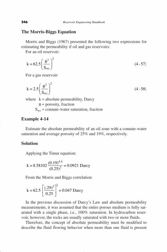
The Morris-Biggs Equation
Morris and Biggs (1967) presented the following two expressions forestimating the permeability if oil and gas reservoirs:
For an oil reservoir:
For a gas reservoir:
where k = absolute permeability, Darcyf = porosity, fraction
Swc = connate-water saturation, fraction
Example 4-14
Estimate the absolute permeability of an oil zone with a connate-watersaturation and average porosity of 25% and 19%, respectively.
Solution
Applying the Timur equation:
From the Morris and Biggs correlation:
In the previous discussion of Darcy’s Law and absolute permeabilitymeasurements, it was assumed that the entire porous medium is fully sat-urated with a single phase, i.e., 100% saturation. In hydrocarbon reser-voir, however, the rocks are usually saturated with two or more fluids.
Therefore, the concept of absolute permeability must be modified todescribe the fluid flowing behavior when more than one fluid is present
k = 62.5 (.29)0.25
= 0.047 Darcy3 2È
ÎÍ
˘
˚˙
k = 8.58102(0.19)(0.25)
= 0.0921 Darcy4.4
2
k = 2.5S
3
wc
fÊËÁ
ˆ¯
2
(4 - 58)
k = 62.5S
3
wc
fÊËÁ
ˆ¯
2
(4 - 57)
246 Reservoir Engineering Handbook
Reservoir Eng Hndbk Ch 04b 2001-10-24 09:46 Page 246

in the reservoir. If a core sample is partially saturated with a fluid (otherthan the test fluid) and both saturations are maintained constant through-out the flow, the measured permeability to the test fluid will be reducedbelow the permeability which could be measured if the core were 100percent saturated with the test fluid.
As the saturation of a particular phase decreases, the permeability tothat phase also decreases. The measured permeability is referred to as theeffective permeability and is a relative measure of the conductance of theporous medium for one fluid when the medium is saturated with morethan one fluid. This implies that the effective permeability is an associat-ed property with each reservoir fluid, i.e., gas, oil, and water. Theseeffective permeabilities for the three reservoir fluids are represented by:
kg = effective gas permeabilityko = effective oil permeabilitykw = effective water permeability
One of the phenomena of multiphase effective permeabilities is thatthe sum of the effective permeabilities is always less than or equal to theabsolute permeability, i.e.,
kg + ko + kw ≤ k
The effective permeability is used mathematically in Darcy’s Law inplace of the absolute permeability. For example, the expression for flowthrough the linear system under a partial saturation of oil is written
where qo = oil flow rate, cc/secmo = oil viscosity, cmko = oil effective permeability, Darcys
Effective permeabilities are normally measured directly in the labora-tory on small core samples. Owing to the many possible combinations ofsaturation for a single medium, however, laboratory data are usuallysummarized and reported as relative permeability. Relative permeabilityis defined as the ratio of the effective permeability to a given fluid at adefinite saturation to the permeability at 100% saturation. The terminolo-
oo 1 2
o
q =k A (p p )
L
-m
(4 - 59)
Fundamentals of Rock Properties 247
Reservoir Eng Hndbk Ch 04b 2001-10-24 09:46 Page 247
gy most widely used is simply kg/k, k0/k, kw/k, meaning the relative per-meability to gas, oil, and water, respectively. Since k is a constant for agiven porous material, the relative permeability varies with the fluid sat-uration in the same fashion as does the effective permeability. The rela-tive permeability to a fluid will vary from a value of zero at some lowsaturation of that fluid to a value of 1.0 at 100% saturation of that fluid.Thus, the relative permeability can be expressed symbolically as
which are relative permeabilities to gas, oil, and water, respectively. Acomprehensive treatment of the relative permeability is presented inChapter 5.
ROCK COMPRESSIBILITY
A reservoir thousands of feet underground is subjected to an overbur-den pressure caused by the weight of the overlying formations. Overbur-den pressures vary from area to area depending on factors such as depth,nature of the structure, consolidation of the formation, and possibly thegeologic age and history of the rocks. Depth of the formation is the mostimportant consideration, and a typical value of overburden pressure isapproximately one psi per foot of depth.
The weight of the overburden simply applies a compressive force tothe reservoir. The pressure in the rock pore spaces does not normallyapproach the overburden pressure. A typical pore pressure, commonlyreferred to as the reservoir pressure, is approximately 0.5 psi per foot ofdepth, assuming that the reservoir is sufficiently consolidated so theoverburden pressure is not transmitted to the fluids in the pore spaces.
The pressure difference between overburden and internal pore pressure isreferred to as the effective overburden pressure. During pressure depletionoperations, the internal pore pressure decreases and, therefore, the effectiveoverburden pressure increases. This increase causes the following effects:
• The bulk volume of the reservoir rock is reduced.• Sand grains within the pore spaces expand.
rgg
roo
rww
k =kk
k = kk
k = kk
248 Reservoir Engineering Handbook
Reservoir Eng Hndbk Ch 04b 2001-10-24 09:46 Page 248

These two volume changes tend to reduce the pore space and, therefore,the porosity of the rock. Often these data exhibit relationships with bothporosity and the effective overburden pressure. Compressibility typicallydecreases with increasing porosity and effective overburden pressure.
Geertsma (1957) points out that there are three different types of com-pressibility that must be distinguished in rocks:
• Rock-matrix compressibility, crIs defined as the fractional change in volume of the solid rock material(grains) with a unit change in pressure. Mathematically, the rock com-pressibility coefficient is given by
where cr = rock-matrix compressibility, psi-1
Vr = volume of solids
The subscript T indicates that the derivative is taken at constant tem-perature.
• Rock-bulk compressibility, cBIs defined as the fractional change in volume of the bulk volume of therock with a unit change in pressure. The rock-bulk compressibility isdefined mathematically by:
where cB = rock-bulk compressibility coefficient, psi-1
VB = bulk volume
• Pore compressibility, cpThe pore compressibility coefficient is defined as the fractional changein pore volume of the rock with a unit change in pressure and given bythe following relationship:
c =1
V
V
ppp
p
T
- ∂∂
ÊËÁ
ˆ¯
(4 - 62)
c =1
VV pB
B
B
T
- ∂∂
ÊËÁ
ˆ¯
(4 - 61)
rr
r
T
c =1
VV p
- ∂∂
ÊËÁ
ˆ¯
(4 - 60)
Fundamentals of Rock Properties 249
Reservoir Eng Hndbk Ch 04b 2001-10-24 09:46 Page 249
where p = pore pressure, psicp = pore compressibility coefficient, psi-1
Vp = pore volume
Equation 4-62 can be expressed in terms of the porosity f by notingthat f increases with the increase in the pore pressure; or:
For most petroleum reservoirs, the rock and bulk compressibility areconsidered small in comparison with the pore compressibility cp. Theformation compressibility cf is the term commonly used to describe thetotal compressibility of the formation and is set equal to cp, i.e.:
Typical values for the formation compressibility range from 3 ¥ 10-6
to 25 ¥ 10-6 psi-1. Equation 4-62 can be rewritten as:
or
DVp = cf VP Dp (4-64)
where DVp and Dp are the change in the pore volume and pore pressure,respectively.
Geertsma (1957) suggested that the bulk compressibility cB is relatedto the pore compressibility cp by the following expression.
cB @ cp f (4-65)
Geertsma has stated that in a reservoir only the vertical component ofhydraulic stress is constant and that the stress components in the horizon-tal plane are characterized by the boundary condition that there is no bulkdeformation in those directions. For those boundary conditions, he devel-oped the following approximation for sandstones:
cp (reservoir) = 1/2 cp (laboratory)
c =1
V
V
pfp
pDD
c c = 1
pf p= ∂∂f
f(4 - 63)
c = 1
pp ff∂
∂
250 Reservoir Engineering Handbook
Reservoir Eng Hndbk Ch 04b 2001-10-24 09:46 Page 250

Example 4-15
Calculate the reduction in the pore volume of a reservoir due to a pres-sure drop of 10 psi. The reservoir original pore volume is one millionbarrels with an estimated formation compressibility of 10 ¥ 10-6 psi-1
Solution
Applying Equation 4-64 gives
DVp = (10 ¥ 10-6) (1 ¥ 106) (10) = 100 bbl
Although the above value is small, it becomes an important factor inundersaturated reservoirs when calculations are made to determine initialoil-in-place and aquifer contents.
The reduction in the pore volume due to pressure decline can also beexpressed in terms of the changes in the reservoir porosity. Equation 4-63can be rearranged, to give:
Integrating the above relation gives:
or:
f = foecf (p - po) (4-66)
where po = original pressure, psifo = original porosityp = current pressure, psif = porosity at pressure p
c p
c p p
f
opo
p
f oo
∂ = ∂
- =ÊËÁ
ˆ¯
ÚÚ ff
ff
f
f
( ) ln
c pf ∂ =ÊËÁ
ˆ¯
∂1f
f
Fundamentals of Rock Properties 251
Reservoir Eng Hndbk Ch 04b 2001-10-24 09:46 Page 251
Noting that the ex expansion series is expressed as:
Using the expansion series and truncating the series after the first twoterms, gives:
f = fo [1 + cf (p - po)] (4-67)
Example 4-16
Given the following data:
• cf = 10 ¥ 10-6
• original pressure = 5000 psi• original porosity = 18%• current pressure = 4500 psi
Calculate the porosity at 4500 psi.
Solution
f = 0.18 [1 + (10 ¥ 10-6)(4500 - 5000)] = 0.179
It should be pointed out that the total reservoir compressibility ct isextensively used in the transient flow equation and the material balanceequation as defined by the following expression:
ct = Soco + Swcs + Sgcg + cf (4-68)
where So, Sw, Sg = oil, water, and gas saturationco = oil compressibility, psi-1
cw = water compressibility, psi-1
cg = gas compressibility, psi-1
ct = total reservoir compressibility
For undersaturated oil reservoirs, the reservoir pressure is above the bub-ble-point pressure, i.e., no initial gas cap, which reduces Equation 4-68 to:
ct = Soco + Swcw + cf
e xx xx = + + + +12 3
2 3
! !. . .
252 Reservoir Engineering Handbook
Reservoir Eng Hndbk Ch 04b 2001-10-24 09:46 Page 252
In general, the formation compressibility cf is the same order of mag-nitude as the compressibility of the oil and water and, therefore, cannotbe regulated.
Several authors have attempted to correlate the pore compressibilitywith various parameters including the formation porosity. Hall (1953)correlated the pore compressibility with porosity as given by the follow-ing relationship:
cf = (1.782/f0.438) 10-6 (4-69)
where cf = formation compressibility, psi-1
f = porosity, fraction
Newman (1973) used 79 samples for consolidated sandstones and lime-stones to develop a correlation between the formation compressibility andporosity. The proposed generalized hyperbolic form of the equation is:
where
For consolidated sandstones
a = 97.32 ¥ 10-6
b = 0.699993c = 79.8181
For limestones
a = 0.8535b = 1.075c = 2.202 ¥ 106
Example 4-17
Estimate the compressibility coefficient of a sandstone formation thatis characterized by a porosity of 0.2, using:
a. Hall’s correlationb. Newman’s correlation
cacbf =
+[ ]1 f
Fundamentals of Rock Properties 253
Reservoir Eng Hndbk Ch 04b 2001-10-24 09:46 Page 253
Solution
a. Hall’s correlations:
cf = (1.782/0.20.438) 10-6 = 3.606 ¥ 10-6 psi-1
b. Newman’s correlation:
NET PAY THICKNESS
A fundamental prerequisite to reservoir performance prediction is asatisfactory knowledge of the volume of oil originally in place. Thereservoir is necessarily confined to certain geologic and fluid boundaries,i.e., GOC, WOC, and GWC, so accuracy is imperative. Within the con-fines of such boundaries, oil is contained in what is commonly referredto as Gross Pay. Net Pay is that part of the reservoir thickness which con-tributes to oil recovery and is defined by imposing the following criteria:
• Lower limit of porosity• Lower limit of permeability• Upper limit of water saturation
All available measurements performed on reservoir samples and inwells, such as core analysis and well logs, are extensively used in evalu-ating the reservoir net thickness.
The choice of lower limits of porosity and permeability will dependupon such individual characteristics as
• Total reservoir volume• Total range of permeability values• Total range of porosity values• Distribution of the permeability and porosity values
c psif = ¥+
= ¥-
- -97 32 10
1 0 699993 79 8181 0 22 74 10
6
1 0 6999936 1.
[ ( . )( . )( . )]./ .
254 Reservoir Engineering Handbook
Reservoir Eng Hndbk Ch 04b 2001-10-24 09:46 Page 254
RESERVOIR HETEROGENEITY
It has been proposed that most reservoirs are laid down in a body ofwater by a long-term process, spanning a variety of depositional environ-ments, in both time and space. As a result of subsequent physical andchemical reorganization, such as compaction, solution, dolomitizationand cementation, the reservoir characteristics are further changed. Thusthe heterogeneity of reservoirs is, for the most part, dependent upon thedepositional environments and subsequent events.
The main geologic characteristic of all the physical rock propertiesthat have a bearing on reservoir behavior when producing oil and gas isthe extreme variability in such properties within the reservoir itself, bothlaterally and vertically, and within short distances. It is important to rec-ognize that there are no homogeneous reservoirs, only varying degrees ofheterogeneity.
The reservoir heterogeneity is then defined as a variation in reservoirproperties as a function of space. Ideally, if the reservoir is homoge-neous, measuring a reservoir property at any location will allow us tofully describe the reservoir. The task of reservoir description is very sim-ple for homogeneous reservoirs. On the other hand, if the reservoir is het-erogeneous, the reservoir properties vary as a function of a spatial loca-tion. These properties may include permeability, porosity, thickness,saturation, faults and fractures, rock facies and rock characteristics. For aproper reservoir description, we need to predict the variation in thesereservoir properties as a function of spatial locations. There are essential-ly two types of heterogeneity:
• Vertical heterogeneity• Areal heterogeneity
Geostatistical methods are used extensively in the petroleum industry toquantitatively describe the two types of the reservoir heterogeneity. It isobvious that the reservoir may be nonuniform in all intensive propertiessuch as permeability, porosity, wettability, and connate water saturation.We will discuss heterogeneity of the reservoir in terms of permeability.
Fundamentals of Rock Properties 255
Reservoir Eng Hndbk Ch 04b 2001-10-24 09:46 Page 255
Vertical Heterogeneity
One of the first problems encountered by the reservoir engineer in pre-dicting or interpreting fluid displacement behavior during secondaryrecovery and enhanced oil recovery processes is that of organizing andusing the large amount of data available from core analysis. Permeabili-ties pose particular problems in organization because they usually varyby more than an order of magnitude between different strata. The engi-neer must be able then to:
• Describe the degree of the vertical heterogeneity in mathematicalterms, and
• Describe and define the proper permeability stratification of the payzone. This task is commonly called the zoning or layering problem.
It is appropriate to be able to describe the degree of heterogeneitywithin a particular system in quantitative terms. The degree of homo-geneity of a reservoir property is a number that characterizes the depar-ture from uniformity or constancy of that particular measured propertythrough the thickness of reservoir. A formation is said to have a uniformi-ty coefficient of zero in a specified property when that property is con-stant throughout the formation thickness. A completely heterogeneousformation has a uniformity coefficient of unity. Between the twoextremes, formations have uniformity coefficients comprised betweenzero and one. The following are the two most widely used descriptors ofthe vertical heterogeneity of the formation:
• Dykstra-Parsons permeability variation V• Lorenz coefficient L
The Dykstra-Parsons Permeability Variation
Dykstra and Parsons (1950) introduced the concept of the permeabilityvariation coefficient V which is a statistical measure of non-uniformity ofa set of data. It is generally applied to the property of permeability butcan be extended to treat other rock properties. It is generally recognizedthat the permeability data are log-normally distributed. That is, the geo-logic processes that create permeability in reservoir rocks appear to leavepermeabilities distributed around the geometric mean. Dykstra and Par-sons recognized this feature and introduced the permeability variationthat characterizes a particular distribution. The required computationalsteps for determining the coefficient V are summarized below:
256 Reservoir Engineering Handbook
Reservoir Eng Hndbk Ch 04b 2001-10-24 09:46 Page 256
Solution
Step 1. Calculate residual liquid saturation Slc.
Slc = Swc + Sorg
= 0.25 + 0.23 = 0.48
Step 2. Generate relative permeability and capillary pressure data for oil-water system by applying Equations 5-22 through 5-24.
kro krw pcSw Equations 5-22 Equation 5-23 Equation 5-24
0.25 0.850 0.000 20.000.30 0.754 0.018 18.190.40 0.557 0.092 14.330.50 0.352 0.198 9.970.60 0.131 0.327 4.570.65 0.000 0.400 0.00
Step 3. Apply Equations 5-25 through 5-27 to determine the relative per-meability and capillary data for the gas-oil system.
kro krg pcSg Equation 5-25 Equation 5-26 Equation 5-27
0.05 0.600 0.000 0.0000.10 0.524 0.248 9.560.20 0.378 0.479 16.760.30 0.241 0.650 21.740.40 0.117 0.796 25.810.52 0.000 0.95 30.00
RELATIVE PERMEABILITY RATIO
Another useful relationship that derives from the relative permeabilityconcept is the relative (or effective) permeability ratio. This quantity lendsitself more readily to analysis and to the correlation of flow performancesthan does relative permeability itself. The relative permeability ratioexpresses the ability of a reservoir to permit flow of one fluid as related toits ability to permit flow of another fluid under the same circumstances.The two most useful permeability ratios are krg/kro the relative permeabili-
298 Reservoir Engineering Handbook
Reservoir Eng Hndbk Ch 05 2001-10-24 09:51 Page 298

ty to gas with respect to that to oil and krw/kro the relative permeability towater with respect to that to oil, it being understood that both quantities inthe ratio are determined simultaneously on a given system. The relativepermeability ratio may vary in magnitude from zero to infinity.
In describing two-phase flow mathematically, it is always the relativepermeability ratio (e.g., krg/kro or kro/krw) that is used in the flow equa-tions. Because the wide range of the relative permeability ratio values,the permeability ratio is usually plotted on the log scale of semilog paperas a function of the saturation. Like many relative permeability ratiocurves, the central or the main portion of the curve is quite linear.
Figure 5-6 shows a plot of krg/kro versus gas saturation. It has becomecommon usage to express the central straight-line portion of the relation-ship in the following analytical form:
The constants a and b may be determined by selecting the coordinateof two different points on the straight-line portion of the curve and sub-stituting in Equation 5-28. The resulting two equations can be solvedsimultaneously for the constants a and b. To find the coefficients ofEquation 5-28 for the straight-line portion of Figure 5-6, select the fol-lowing two points:
Point 1: at Sg = 0.2, the relative permeability ratio krg/kro = 0.07Point 2: at Sg = 0.4, the relative permeability ratio krg/kro = 0.70
Imposing the above points on Equation 5-28, gives:
0.07 = a e0.2b
0.70 = a e0.4b
Solving simultaneously gives:
• The intercept a = 0.0070• The slope b = 11.513
k
ka erg
ro
bSg= (5 - 28)
Relative Permeability Concepts 299
Reservoir Eng Hndbk Ch 05 2001-10-24 09:51 Page 299
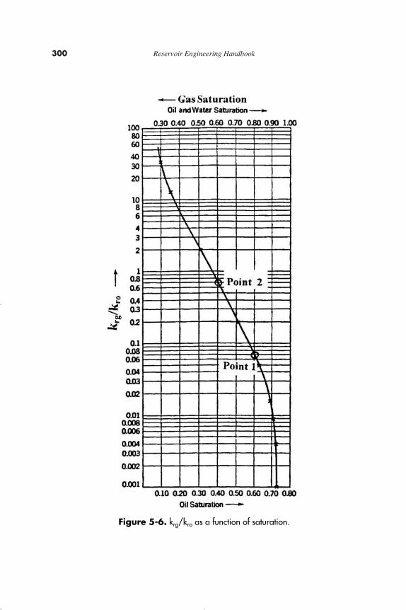
300 Reservoir Engineering Handbook
Figure 5-6. krg/kro as a function of saturation.
Reservoir Eng Hndbk Ch 05 2001-10-24 09:51 Page 300
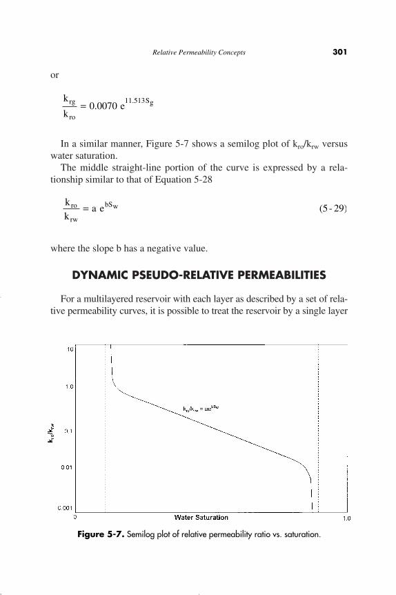
or
In a similar manner, Figure 5-7 shows a semilog plot of kro/krw versuswater saturation.
The middle straight-line portion of the curve is expressed by a rela-tionship similar to that of Equation 5-28
where the slope b has a negative value.
DYNAMIC PSEUDO-RELATIVE PERMEABILITIES
For a multilayered reservoir with each layer as described by a set of rela-tive permeability curves, it is possible to treat the reservoir by a single layer
kk
a ero
rw
bSw= (5 - 29)
k
kerg
ro
Sg= 0 007011 513
..
Relative Permeability Concepts 301
Figure 5-7. Semilog plot of relative permeability ratio vs. saturation.
Reservoir Eng Hndbk Ch 05 2001-10-24 09:51 Page 301
that is characterized by a weighted-average porosity, absolute permeability,and a set of dynamic pseudo-relative permeability curves. These averagingproperties are calculated by applying the following set of relationships:
Average Porosity
Average Absolute Permeability
Average Relative Permeability for the Wetting Phase
Average Relative Permeability for the Nonwetting Phase
The corresponding average saturations should be determined by usingEquations 4-16 through 4-18. These equations are given below for con-venience:
k
k h k
k hrnw
i rnw ii
N
ii
N= =
=
Â
Â
( ) ( )
( )
1
1
(5 - 33)
k
k h k
k hrw
i rw ii
N
ii
N= =
=
Â
Â
( ) ( )
( )
1
1
(5 - 32)
k
k h
havg
i ii
N
i
= =Â
Â1 (5 - 31)
ff
avg
ii
N
i
i
h
h= =
ÂÂ1 (5 - 30)
302 Reservoir Engineering Handbook
Reservoir Eng Hndbk Ch 05 2001-10-24 09:51 Page 302

Average Oil Saturation
Average Water Saturation
Average Gas Saturation
where n = total number of layershi = thickness of layer iki = absolute permeability of layer i
krw = average relative permeability of the wetting phasekrnw = average relative permeability of the nonwetting phase
In Equations 5-22 and 5-23, the subscripts w and nw represent wettingand nonwetting, respectively. The resulting dynamic pseudo-relative per-meability curves are then used in a single-layer model. The objective ofthe single-layer model is to produce results similar to those from the mul-tilayered, cross-sectional model.
gi = 1
n
i i ig
i = 1
n
i i
S =
h S
h
Â
Â
f
f
S =
h S
hw
i = 1
n
i i iw
i = 1
n
i i
Â
Â
f
f
oi = 1
n
i i io
i = 1
n
i i
S =
h S
h
Â
Â
f
f
Relative Permeability Concepts 303
Reservoir Eng Hndbk Ch 05 2001-10-24 09:52 Page 303

NORMALIZATION AND AVERAGINGRELATIVE PERMEABILITY DATA
Results of relative permeability tests performed on several core sam-ples of a reservoir rock often vary. Therefore, it is necessary to averagethe relative permeability data obtained on individual rock samples. Priorto usage for oil recovery prediction, the relative permeability curvesshould first be normalized to remove the effect of different initial waterand critical oil saturations. The relative permeability can then be de-nor-malized and assigned to different regions of the reservoir based on theexisting critical fluid saturation for each reservoir region.
The most generally used method adjusts all data to reflect assignedend values, determines an average adjusted curve and finally constructsan average curve to reflect reservoir conditions. These procedures arecommonly described as normalizing and de-normalizing the relative per-meability data.
To perform the normalization procedure, it is helpful to set up the cal-culation steps for each core sample i in a tabulated form as shown below:
Relative Permeability Data for Core Sample i
(1) (2) (3) (4) (5) (6)
Sw kro krw
The following normalization methodology describes the necessarysteps for a water-oil system as outlined in the above table.
Step 1. Select several values of Sw starting at Swc (column 1), and list thecorresponding values of kro and krw in columns 2 and 3.
Step 2. Calculate the normalized water saturation S*w for each set of rela-
tive permeability curves and list the calculated values in column 4by using the following expression:
SS S
S Sw
w wc
wc oc
* = -- -1
(5 - 34)
kk
krw
rw
rw Soc
*
( )=k
kk
roro
ro Swc
*
( )=S
S S
S Sw
w wc
wc oc
* =-
- -1
304 Reservoir Engineering Handbook
Reservoir Eng Hndbk Ch 05 2001-10-24 09:52 Page 304

where Soc = critical oil saturationSwc = connate water saturationS*
w = normalized water saturation
Step 3. Calculate the normalized relative permeability for the oil phase atdifferent water saturation by using the relation (column 5):
where kro = relative permeability of oil at different Sw
(kro)Swc = relative permeability of oil at connate watersaturation
k*ro = normalized relative permeability of oil
Step 4. Normalize the relative permeability of the water phase by apply-ing the following expression and document results of the calcula-tion in column 6
where (krw)Soc is the relative permeability of water at the criticaloil saturation.
Step 5. Using regular Cartesian coordinate, plot the normalized k*ro and
k*rw versus S*
w for all core samples on the same graph.
Step 6. Determine the average normalized relative permeability valuesfor oil and water as a function of the normalized water saturationby select arbitrary values of S*
w and calculate the average of k*ro
and k*rw by applying the following relationships:
( )
( )
( )
*
*
k
h k k
h kro avg
ro ii
n
ii
n= =
=
Â
Â1
1
(5 - 37)
kkkrw
rw
rw Soc
*
( )= (5 - 36)
kk
kroro
ro Swc
*
( )= (5 - 35)
Relative Permeability Concepts 305
Reservoir Eng Hndbk Ch 05 2001-10-24 09:52 Page 305
where n = total number of core sampleshi = thickness of sample iki = absolute permeability of sample i
Step 7. The last step in this methodology involves de-normalizing theaverage curve to reflect actual reservoir and conditions of Swc andSoc. These parameters are the most critical part of the methodologyand, therefore, a major effort should be spent in determining repre-sentative values. The Swc and Soc are usually determined by aver-aging the core data, log analysis, or correlations, versus graphs,such as: (kro)Swc vs. Swc, (krw)Soc vs. Soc, and Soc vs. Swc whichshould be constructed to determine if a significant correlationexists. Often, plots of Swc and Sor versus log Zk/f may demon-strate a reliable correlation to determine end-point saturations asshown schematically in Figure 5-8. When representative end val-ues have been estimated, it is again convenient to perform the de-normalization calculations in a tabular form as illustrated below:
(1) (2) (3) (4) (5) (6)
S*w (k*
ro)avg (k*rw)avg Sw = S*
w (1 - Swc - Soc) + Swc kro = (k*ro)avg (k
–ro)Swc krw = (k*
rw)avg (k–
rw)Soc
Where (kro)Swc and (kro)Soc are the average relative permeability of oiland water at connate water and critical oil, respectively, and given by:
( )
( )
( )
k
h k k
h k
rw Soc
rw Soc ii
n
ii
n=[ ]
=
=
Â
Â1
1
(5 - 40)
( )
( )
( )
k
h k k
h k
ro Swc
ro Swc ii
n
ii
n=[ ]
-
=
Â
Â1
1
(5 - 39)
( )
( )
( )
*
*
k
h k k
h krw avg
rw ii
n
ii
n= =
=
Â
Â1
1
(5 - 38)
306 Reservoir Engineering Handbook
Reservoir Eng Hndbk Ch 05 2001-10-24 09:52 Page 306

Example 5-6
Relative permeability measurements are made on three core samples.The measured data are summarized below:
Core Sample #1 Core Sample #2 Core Sample #3
h = 1ft h = 1 ft h = 1 ftk = 100 md k = 80 md k = 150 mdSoc = 0.35 Soc = 0.28 Soc = 0.35Swc = 0.25 Swc = 0.30 Swc = 0.20
Sw kro krw kro krw kro krw
0.20 — — — — 1.000* 0.0000.25 0.850* 0.000 — — 0.872 0.0080.30 0.754 0.018 0.800 0 0.839 0.0270.40 0.557 0.092 0.593 0.077 0.663 0.0880.50 0.352 0.198 0.393 0.191 0.463 0.1760.60 0.131 0.327 0.202 0.323 0.215 0.2860.65 0.000 0.400* 0.111 0.394 0.000 0.350*0.72 — — 0.000 0.500* — —
*Values at critical saturations
It is believed that a connate water saturation of 0.27 and a critical oilsaturation of 30% better describe the formation. Generate the oil andwater relative permeability data using the new critical saturations.
Relative Permeability Concepts 307
Figure 5-8. Critical saturation relationships.
Reservoir Eng Hndbk Ch 05 2001-10-24 09:52 Page 307

Solution
Step 1. Calculate the normalized water saturation for each core sample byusing Equation 5-36.
Core Sample #1 Core Sample #2 Core Sample #3S*w S*w S*w S*w
0.20 — — 0.0000.25 0.000 — 0.1110.30 0.125 0.000 0.2220.40 0.375 0.238 0.4440.50 0.625 0.476 0.6670.60 0.875 0.714 0.8890.65 1.000 0.833 1.0000.72 — 1.000 —
Step 2. Determine relative permeability values at critical saturation foreach core sample.
Core 1 Core 2 Core 3
(kro)Swc 0.850 0.800 1.000(krw)Sor 0.400 0.500 0.35
Step 3. Calculate (k–ro)Swc and (k–rw)Sor by applying Equations 5-39 and5-40 to give:
(k–ro)Swc = 0.906
(k–rw)Soc = 0.402
Step 4. Calculate the normalized k*ro and k*
rw for all core samples:
Core 1 Core 2 Core 3Sw S*w k*ro k*rw S*w k*ro k*rw S*w k*ro k*rw
0.20 — — — — — — 0.000 1.000 00.25 0.000 1.000 0 — — — 0.111 0.872 0.0230.30 0.125 0.887 0.045 0.000 1.000 0 0.222 0.839 0.0770.40 0.375 0.655 0.230 0.238 0.741 0.154 0.444 0.663 0.2510.50 0.625 0.414 0.495 0.476 0.491 0.382 0.667 0.463 0.5030.60 0.875 0.154 0.818 0.714 0.252 0.646 0.889 0.215 0.8170.65 1.000 0.000 1.000 0.833 0.139 0.788 1.000 0.000 1.0000.72 — — — 1.000 0.000 1.000 — — —
308 Reservoir Engineering Handbook
Reservoir Eng Hndbk Ch 05 2001-10-24 09:52 Page 308
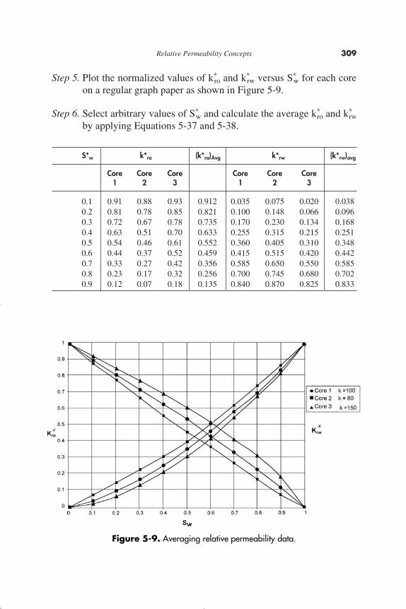
Step 5. Plot the normalized values of k*ro and k*
rw versus S*w for each core
on a regular graph paper as shown in Figure 5-9.
Step 6. Select arbitrary values of S*w and calculate the average k*
ro and k*rw
by applying Equations 5-37 and 5-38.
S*w k*ro (k*ro)Avg k*rw (k*rw)avg
Core Core Core Core Core Core1 2 3 1 2 3
0.1 0.91 0.88 0.93 0.912 0.035 0.075 0.020 0.0380.2 0.81 0.78 0.85 0.821 0.100 0.148 0.066 0.0960.3 0.72 0.67 0.78 0.735 0.170 0.230 0.134 0.1680.4 0.63 0.51 0.70 0.633 0.255 0.315 0.215 0.2510.5 0.54 0.46 0.61 0.552 0.360 0.405 0.310 0.3480.6 0.44 0.37 0.52 0.459 0.415 0.515 0.420 0.4420.7 0.33 0.27 0.42 0.356 0.585 0.650 0.550 0.5850.8 0.23 0.17 0.32 0.256 0.700 0.745 0.680 0.7020.9 0.12 0.07 0.18 0.135 0.840 0.870 0.825 0.833
Relative Permeability Concepts 309
Figure 5-9. Averaging relative permeability data.
Reservoir Eng Hndbk Ch 05 2001-10-24 09:52 Page 309
Step 7. Using the desired formation Soc and Swc (i.e., Soc = 0.30, Swc =0.27), de-normalize the data to generate the required relative per-meability data as shown below:
S*w (k*ro)avg (k*rw)avg Sw = S*w (1 - Swc - Soc) kro = 0.906 krw = 0.402+ Swc (k*ro)avg (k*rw)avg
0.1 0.912 0.038 0.313 0.826 0.0150.2 0.821 0.096 0.356 0.744 0.0390.3 0.735 0.168 0.399 0.666 0.0680.4 0.633 0.251 0.442 0.573 0.1010.5 0.552 0.368 0.485 0.473 0.1400.6 0.459 0.442 0.528 0.416 0.1780.7 0.356 0.585 0.571 0.323 0.2350.8 0.256 0.702 0.614 0.232 0.2820.9 0.135 0.833 0.657 0.122 0.335
It should be noted that the proposed normalization procedure forwater-oil systems as outlined above could be extended to other systems,i.e., gas-oil or gas-water.
THREE-PHASE RELATIVE PERMEABILITY
The relative permeability to a fluid is defined as the ratio of effectivepermeability at a given saturation of that fluid to the absolute permeabili-ty at 100% saturation. Each porous system has unique relative permeabil-ity characteristics, which must be measured experimentally. Direct exper-imental determination of three-phase relative permeability properties isextremely difficult and involves rather complex techniques to determinethe fluid saturation distribution along the length of the core. For this rea-son, the more easily measured two-phase relative permeability character-istics are experimentally determined.
In a three-phase system of this type it is found that the relative perme-ability to water depends only upon the water saturation. Since the watercan flow only through the smallest interconnect pores that are present inthe rock and able to accommodate its volume, it is hardly surprising thatthe flow of water does not depend upon the nature of the fluids occupy-ing the other pores. Similarly, the gas relative permeability depends onlyupon the gas saturation. This fluid, like water, is restricted to a particularrange of pore sizes and its flow is not influenced by the nature of thefluid or fluids that fill the remaining pores.
310 Reservoir Engineering Handbook
Reservoir Eng Hndbk Ch 05 2001-10-24 09:52 Page 310

The pores available for flow of oil are those that, in size, are largerthan pores passing only water, and smaller than pores passing only gas.The number of pores occupied by oil depends upon the particular sizedistribution of the pores in the rock in which the three phases coexist andupon the oil saturation itself.
In general, the relative permeability of each phase, i.e., water, gas, andoil, in a three-phase system is essentially related to the existing saturationby the following functions:
krw = f (Sw) (5-41)
krg = f (Sg) (5-42)
kro = f (Sw, Sg) (5-43)
Function 5-43 is rarely known and, therefore, several practicalapproaches are proposed and based on estimating the three-phase relativepermeability from two sets of two-phase data:
Set 1: Oil-Water System
krow = f (Sw)
krw = f (Sw)
Set 2: Oil-Gas System
krog = f (Sg)
krg = f (Sg)
where krow and krog are defined as the relative permeability to oil in thewater-oil two-phase system and similarly krog is the relative permeabilityof oil in the gas-oil system. The symbol kro is reserved for the oil relativepermeability in the three-phase system.
The triangular graph paper is commonly used to illustrate the changes inthe relative permeability values when three phases are flowing simultane-ously, as illustrated in Figures 5-10 and 5-11. The relative permeabilitydata are plotted as lines of constant percentage relative permeability (oil,water, and gas isoperms). Figures 5-10 and 5-11 show that the relative per-meability data, expressed as isoperms, are dependent on the saturation val-ues for all three phases in the rock.
Relative Permeability Concepts 311
Reservoir Eng Hndbk Ch 05 2001-10-24 09:52 Page 311

Three-Phase Relative Permeability Correlations
Honarpour, Keoderitz, and Harvey (1988) provided a comprehensivetreatment of the two- and three-phase relative permeabilities. The authorslisted numerous correlations for estimating relative permeabilities. Thesimplest approach to predict the relative permeability to the oil phase in athree-phase system is defined as:
kro = krowkrog (5-44)
There are several practical and more accurate correlations that havedeveloped over the years, including:
• Wyllie’s Correlations• Stone’s Model I• Stone’s Model II• The Hustad-Holt Correlation
312 Reservoir Engineering Handbook
Figure 5-10. Three-plate relative permeability imbibition. (After Honarpour et al., 1988.)
Reservoir Eng Hndbk Ch 05 2001-10-24 09:52 Page 312
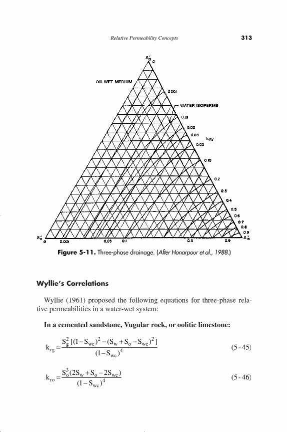
Wyllie’s Correlations
Wyllie (1961) proposed the following equations for three-phase rela-tive permeabilities in a water-wet system:
In a cemented sandstone, Vugular rock, or oolitic limestone:
kS S S S
Sroo w o wc
wc
= + --
3
42 2
1
( )
( )(5 - 46)
kS S S S S
Srgg wc w o wc
wc
=- - + -
-
2 2 2
4
1
1
[( ) ( ) ]
( )(5 - 45)
Relative Permeability Concepts 313
Figure 5-11. Three-phase drainage. (After Honarpour et al., 1988.)
Reservoir Eng Hndbk Ch 05 2001-10-24 09:52 Page 313
In unconsolidated, well-sorted sand:
Stone’s Model I
Stone (1970) developed a probability model to estimate three-phaserelative permeability data from the laboratory-measured two-phase data.The model combines the channel flow theory in porous media with prob-ability concepts to obtain a simple result for determining the relative per-meability to oil in the presence of water and gas flow. The modelaccounts for hysteresis effects when water and gas saturations are chang-ing in the same direction of the two sets of data.
The use of the channel flow theory implies that water-relative perme-ability and water-oil capillary pressure in the three-phase system are func-tions of water saturation alone, irrespective of the relative saturations ofoil and gas. Moreover, they are the same function in the three-phase sys-tem as in the two-phase water-oil system. Similarly, the gas-phase relativepermeability and gas-oil capillary pressure are the same functions of gassaturation in the three-phase system as in the two-phase gas-oil system.
Stone suggested that a nonzero residual oil saturation, called minimumoil saturation, Som exists when oil is displaced simultaneously by waterand gas. It should be noted that this minimum oil saturation Som is differ-ent than the critical oil saturation in the oil-water system (i.e., Sorw) andthe residual oil saturation in the gas-oil system, i.e., Sorg. Stone intro-duced the following normalized saturations:
kS S S S
Srgo w o wc
wi
= + --
( ) ( )
( )
3 4
42 2
1(5 - 50)
kS
Sroo
wc
=-( )
( )
3
31(5 - 49)
kS S
Srww wc
wi= -
-ÊËÁ
ˆ¯1
3
(5 - 48)
kS S
Srww wc
wc= -
-ÊËÁ
ˆ¯1
4
(5 - 47)
314 Reservoir Engineering Handbook
Reservoir Eng Hndbk Ch 05 2001-10-24 09:52 Page 314
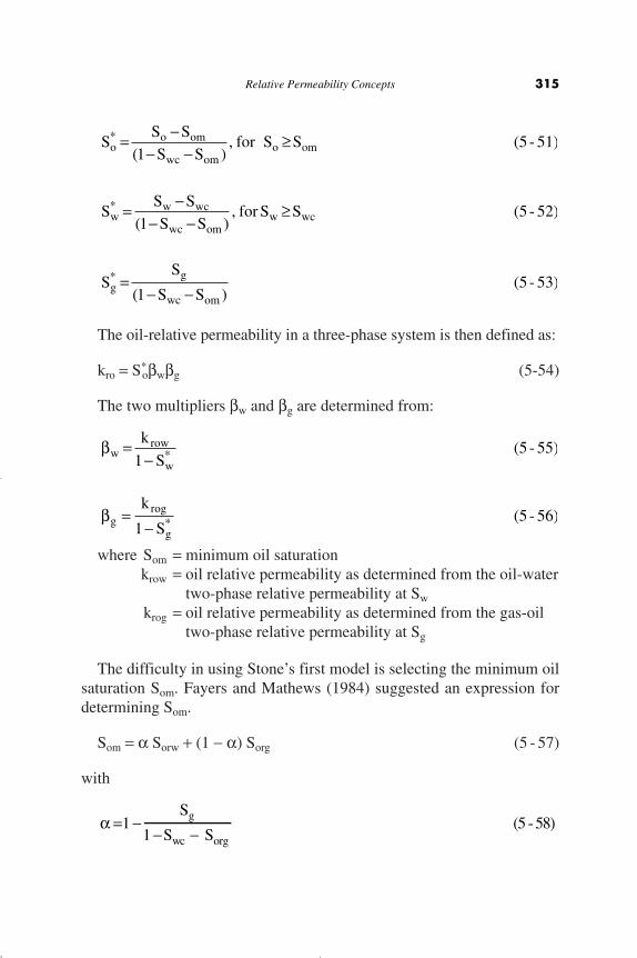
The oil-relative permeability in a three-phase system is then defined as:
kro = S*obwbg (5-54)
The two multipliers bw and bg are determined from:
where Som = minimum oil saturationkrow = oil relative permeability as determined from the oil-water
two-phase relative permeability at Sw
krog = oil relative permeability as determined from the gas-oiltwo-phase relative permeability at Sg
The difficulty in using Stone’s first model is selecting the minimum oilsaturation Som. Fayers and Mathews (1984) suggested an expression fordetermining Som.
Som = a Sorw + (1 - a) Sorg (5 - 57)
with
a =1 -Sg
1 -Swc - Sorg(5 -58)
bgrog
g
k
S=
-1 * (5 - 56)
bwrow
w
k
S=
-1 * (5 - 55)
SS
S Sgg
wc om
*
( )=
- -1(5 - 53)
SS SS S
for S Sww wc
wc omw wc
*
( ),= -
- -≥
1(5 - 52)
SS SS S
for S Soo om
wc omo om
*
( ),= -
- -≥
1(5 - 51)
Relative Permeability Concepts 315
Reservoir Eng Hndbk Ch 05 2001-10-24 09:52 Page 315
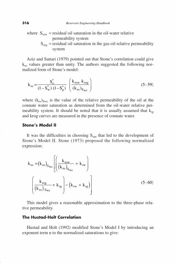
where Sorw = residual oil saturation in the oil-water relativepermeability system
Sorg = residual oil saturation in the gas-oil relative permeabilitysystem
Aziz and Sattari (1979) pointed out that Stone’s correlation could givekro values greater than unity. The authors suggested the following nor-malized form of Stone’s model:
where (kro)Swc is the value of the relative permeability of the oil at theconnate water saturation as determined from the oil-water relative per-meability system. It should be noted that it is usually assumed that krg
and krog curves are measured in the presence of connate water.
Stone’s Model II
It was the difficulties in choosing Som that led to the development ofStone’s Model II. Stone (1973) proposed the following normalizedexpression:
This model gives a reasonable approximation to the three-phase rela-tive permeability.
The Hustad-Holt Correlation
Hustad and Holt (1992) modified Stone’s Model I by introducing anexponent term n to the normalized saturations to give:
k kk
kk
k
kk k k
ro ro Swcrow
ro Swc
rw
rog
ro Swcrg rw rg
= ( ) ( ) +Ê
ËÁÁ
ˆ
¯˜
È
Î
ÍÍ
( ) +Ê
Ë
ÁÁ
ˆ
¯
˜˜
- +( )˘
˚
˙˙˙
(5 - 60)
kS
S S
k k
kroo
w g
row rog
ro Swc
=- -
Ê
ËÁ
ˆ
¯˜*
*
*( ) ( ) ( )1 1(5 - 59)
316 Reservoir Engineering Handbook
Reservoir Eng Hndbk Ch 05 2001-10-24 09:52 Page 316
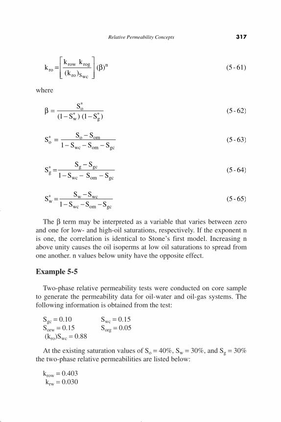
where
The b term may be interpreted as a variable that varies between zeroand one for low- and high-oil saturations, respectively. If the exponent nis one, the correlation is identical to Stone’s first model. Increasing nabove unity causes the oil isoperms at low oil saturations to spread fromone another. n values below unity have the opposite effect.
Example 5-5
Two-phase relative permeability tests were conducted on core sampleto generate the permeability data for oil-water and oil-gas systems. Thefollowing information is obtained from the test:
Sgc = 0.10 Swc = 0.15Sorw = 0.15 Sorg = 0.05(kro)Swc = 0.88
At the existing saturation values of So = 40%, Sw = 30%, and Sg = 30%the two-phase relative permeabilities are listed below:
krow = 0.403krw = 0.030
SS S
S S Sww wc
wc om gc
* = -- - -1
(5 - 65)
SS S
S S Sgg gc
wc om gc
* =-
- - -1(5 - 64)
SS S
S S Soo om
wc om gc
* = -- - -1
(5 - 63)
b =- -
*
* *S
S So
w g( ) ( )1 1(5 - 62)
kk k
krorow rog
ro Swc
n=È
ÎÍÍ
˘
˚˙˙( )
( )b (5 - 61)
Relative Permeability Concepts 317
Reservoir Eng Hndbk Ch 05 2001-10-24 09:52 Page 317

krg = 0.035krog = 0.175
Estimate the three-phase relative permeability at the existing satura-tions by using:
a. Stone’s Model Ib. Stone’s Model II
Solution
a. Stone’s Model I
Step 1. Calculate Som by applying Equations 5-58 and 5-57, to give:
Som = (0.625) (0.15) + (1 - 0.625) (0.05) = 0.1125
Step 2. Calculate the normalized saturations by applying Equations 5-51through 5-53.
Step 3. Estimate kro by using Equation 5-59.
b. Stone’s Model II
Apply Equation 5-60 to give:
kro =- -
ÈÎÍ
˘˚
=0 38981 0 2034 1 0 4068
0 406 0 1750 88
0 067.
( . ) ( . )( . ) ( . )
..
Sg* =
- -=0 3
1 0 15 0 11250 4068
.. .
.
Sw* = -
- -=0 30 0 15
1 0 15 0 11250 2034
. .. .
.
So* = -
- -=0 4 0 1125
1 0 15 0 11250 3898
. .. .
.
a = -- -
=10 3
1 0 15 0 050 625
.. .
.
318 Reservoir Engineering Handbook
Reservoir Eng Hndbk Ch 05 2001-10-24 09:52 Page 318

PROBLEMS
1. Given:
• Swc = 0.30 Sgc = 0.06 Soc = 0.35• unconsolidated-well sorted sand
Generate the drainage relative permeability data by using:
a. The Wyllie-Gardner correlationb. Pirson’s correlationc. Corey’s method
2. The capillary pressure data for an oil-water system are given below:
Sw pc, psi
0.25 350.30 160.40 8.50.50 51.00 0
a. Generate the relative permeability data for this system.b. Using the relative permeability ratio concept, plot kro/krw versus Sw
on a semi-log scale and determine the coefficients of the followingexpression:
kro/krw = aebSw
3. Using the relative permeability data of Example 5-6, generate the rela-tive permeability values for a layer in the reservoir that is character-ized by the following critical saturations:
Soc = 0.25 Swc = 0.25 h = 1
4. Prepare a krg/kro versus Sg plot for the following laboratory data:
krg/kro Sg
1.9 0.500.109 0.30
kro = +ÊË
ˆ¯ +Ê
ˈ¯ - +È
Î͢˚
=0 880 4060 88
0 030 1750 88
0 035 0 03 0 035 0 044...
...
. ( . . ) .
Relative Permeability Concepts 319
Reservoir Eng Hndbk Ch 05 2001-10-24 09:52 Page 319
Find the coefficients of the following relationship:
krg/kro = aeb Sg
REFERENCES
1. Aziz, K., and Sattari, A., Petroleum Reservoir Simulation. London: AppliedScience Publishers Ltd., 1979.
2. Corey, A. T., and Rathjens, C. H., “Effect of Stratification on Relative Per-meability,” Trans. AIME, 1956, pp. 207, 358.
3. Corey, A. T., “The Interrelation Between Gas and Oil Relative Permeabili-ties,” Prod. Mon., 1954, pp. 19, 38, 1954.
4. Fayers, F., and Matthews, J. D., “Evaluation of Normalized Stone’s Methodfor Estimating Three-Phase Relative Permeabilities,” SPEJ, April 1984, pp.224–239.
5. Honarpour, M. M., Koederitz, L. F., and Harvey, A. H., “Empirical Equa-tions for Estimating Two-Phase Relative Permeability in ConsolidatedRock,” Trans. AIME, 1982, pp. 273, 290.
6. Honarpour, M. M., Koederitz, L. F., and Harvey, A. H., Relative Permeabili-ty of Petroleum Reservoirs. CRC Press, Inc., 1988.
7. Hustad, O. S., and Holt, T., “Gravity Stable Displacement of Oil by Hydro-carbon Gas after Waterflooding,” SPE Paper 24116, EOR Symposium,Tulsa, OK, 1992.
8. Pirson, S. J. (ed.), Oil Reservoir Engineering. New York: McGraw-Hill, 1958.
9. Rose, W. D., and Bruce, W. A., “Evaluation of Capillary Character in Petro-leum Reservoir Rock,” Trans. AIME, 1949, pp. 127, 186.
10. Stone, H. L., “Estimation of Three-Phase Relative Permeability and ResidualOil Data, “ J. of Can. Pet. Technol., 1973, pp. 12, 53.
11. Stone, H. L., “Estimation of Three-Phase Relative Permeability, JPT, 1970,pp. 2, 214.
12. Torcaso, M. A., and Wyllie, M. R. J., “A Comparison of Calculated krg/kro
Ratios with Field Data,” JPT, 1958, pp. 6, 57.
13. Wyllie, M.R.J., and Gardner, G.H.F., “The Generalized Kozeny-CarmenEquation—Its Application to Problems of Multi-Phase Flow in PorousMedia,” World Oil, 1958, pp.121, 146.
14. Wyllie, M.R.J., “Interrelationship Between Wetting and Nonwetting PhaseRelative Permeability,” Trans. AIME, 1961, pp. 83, 192.
320 Reservoir Engineering Handbook
Reservoir Eng Hndbk Ch 05 2001-10-24 09:52 Page 320


![Low-pressure hydrocephalus: A case report · 2015-06-22 · Hydrocephalus is a pathological increase in the CSF volume, regardless of hydrostatic or barometric pressure [1]. Normal](https://img.pdfslide.us/doc/110x75/5f932f5774b0c262f97f04f4/low-pressure-hydrocephalus-a-case-report-2015-06-22-hydrocephalus-is-a-pathological.jpg)