Seasonal Effects of Indian Ocean Freshwater Forcing in …iprc.soest.hawaii.edu/users/xie/hyodae-BL09.pdf · Seasonal Effects of Indian Ocean Freshwater Forcing in a Regional Coupled

Seasonal Effects of Indian Ocean Freshwater Forcing in a Regional Coupled Model*

HYODAE SEO

International Pacific Research Center, University of Hawaii at Manoa, Honolulu, Hawaii

SHANG-PING XIE

International Pacific Research Center, and Department of Meteorology, University of Hawaii at Manoa, Honolulu, Hawaii

RAGHU MURTUGUDDE

Earth System Science Interdisciplinary Center, Department of Atmospheric and Oceanic Science,

University of Maryland, College Park, College Park, Maryland

MARKUS JOCHUM

National Center for Atmospheric Research, Boulder, Colorado

ARTHUR J. MILLER

Scripps Institution of Oceanography, University of California, San Diego, La Jolla, California

(Manuscript received 16 December 2008, in final form 30 July 2009)

ABSTRACT

Effects of freshwater forcing from river discharge into the Indian Ocean on oceanic vertical structure and

the Indian monsoons are investigated using a fully coupled, high-resolution, regional climate model. The

effect of river discharge is included in the model by restoring sea surface salinity (SSS) toward observations.

The simulations with and without this effect in the coupled model reveal a highly seasonal influence of salinity

and the barrier layer (BL) on oceanic vertical density stratification, which is in turn linked to changes in sea

surface temperature (SST), surface winds, and precipitation.

During both boreal summer and winter, SSS relaxation leads to a more realistic spatial distribution of

salinity and the BL in the model. In summer, the BL in the Bay of Bengal enhances the upper-ocean strat-

ification and increases the SST near the river mouths where the freshwater forcing is largest. However, the

warming is limited to the coastal ocean and the amplitude is not large enough to give a significant impact on

monsoon rainfall.

The strengthened BL during boreal winter leads to a shallower mixed layer. Atmospheric heat flux forcing

acting on a thin mixed layer results in an extensive reduction of SST over the northern Indian Ocean. Rel-

atively suppressed mixing below the mixed layer warms the subsurface layer, leading to a temperature

inversion. The cooling of the sea surface induces a large-scale adjustment in the winter atmosphere with

amplified northeasterly winds. This impedes atmospheric convection north of the equator while facilitating it

in the austral summer intertropical convergence zone, resulting in a hemispheric-asymmetric response pat-

tern. Overall, the results suggest that freshwater forcing from the river discharges plays an important role

during the boreal winter by affecting SST and the coupled ocean–atmosphere interaction, with potential

impacts on the broadscale regional climate.

* International Pacific Research Center Publication Number 626 and School of Ocean and Earth Science and Technology Publication

Number 7788.

Corresponding author address: Hyodae Seo, International Pacific Research Center, University of Hawaii at Manoa, 1680 East-West

Road, POST Bldg., #401, Honolulu, HI 96822.

E-mail: [email protected]

15 DECEMBER 2009 S E O E T A L . 6577

DOI: 10.1175/2009JCLI2990.1

1. Introduction

The Bay of Bengal (BoB) receives substantial fresh-

water flux from both local precipitation and river dis-

charge during the summer southwest (SW) monsoon.

Precipitation well exceeds evaporation (Harenduprakash

and Mitra 1988; Prasad 1997). In addition, major rivers

from the bordering countries—the Irrawaddy, the Krishna,

the Godavari, the Mahanadi, the Ganges, and the

Brahmaputra—discharge an annual freshwater volume

into the BoB, whose estimates vary between 1.5 3 1012 m3

(Thadathil et al. 2002) and 1.83 3 1013 m3 (Varkey et al.

1996), making the BoB the freshest region in the Indian

Ocean. Seasonally, three-fourths of all riverine influx

occurs during the SW monsoon period from May until

September, indicating that this substantial summertime

freshwater influx will affect the hydrography of the bay

during the northeast (NE) monsoon (Shetye et al. 1996).

The unique summertime and wintertime oceanic con-

ditions associated with the presence of a low-salinity

layer lead to marked variations in density stratifica-

tion and vertical mixing in the BoB both in summer

(Vinayachandran et al. 2002) and winter (Shetye et al.

1996). The strong halocline associated with the surface

freshwater cap shoals the density mixed layer (ML),

while the isothermal layer depth (ILD) is usually

deeper. Thus salinity has a crucial control on the depth

to which mixing effects are confined. The ILD is defined

in this study as the depth at which temperature drops

from sea surface temperature (SST) by DT 5 18C. The

ML depth (MLD) is defined as the depth at which the

salinity effect on the density variation is equivalent to

the variation of temperature by DT 5 18C from the sea

surface. Following the criterion of Sprintall and Tomczak

(1992), the positive difference in the MLD and ILD is

termed the barrier layer (BL) (Lukas and Lindstrom

1991) since it acts as a barrier to the mixing of cold

thermocline water into the surface ML, essentially de-

coupling the dynamics and the thermodynamics. That is,

the stratified BL retains atmospheric heat and momen-

tum inputs predominantly within the ML while reducing

the entrainment of the cooler thermocline water from

the bottom (Vialard and Delecluse 1998). A survey of

BL thickness (BLT) by Sprintall and Tomczak (1992)

using the Levitus (1982) climatology indicates that BLs

exist throughout the year in the BoB, with a thickness

of 25 m during August–October in the northwestern

part of the bay (Vinayachandran et al. 2002). Rao and

Sivakumar (2003) also discuss the formation mechanism

and seasonal cycle of the BL in the northern Indian

Ocean. They showed that the build up of the BL during

summertime becomes most prominent by February in the

following year, reaching a maximum thickness of 50 m.

The boreal winter is the period when the hydrological

forcing generates its largest freshening effects through

the river discharge and local rainfall. The BLT sub-

sequently diminishes from February to a minimum in

May before onset of the summer monsoon. Based on

more recent datasets with better spatial and temporal

coverage, various investigators confirm the seasonal

cycle and observed thickness of the BL in the BoB and

northern Indian Ocean (e.g., Thadathil et al. 2007;

Mignot et al. 2007; de Boyer Montegut et al. 2007,

hereafter DMLC07).

High SST in the BoB is conducive to deep convection

in the atmosphere and hence precipitation during the SW

monsoon season (Gadgil et al. 1984; Shenoi et al. 2002).

Altered atmospheric convection results in variations in

air–sea heat flux, which can further influence the con-

vection itself via SST changes (Krishnamurti et al. 1988).

Furthermore, through the aforementioned impact of the

BL on ocean mixing, surface freshwater affects SST

and ocean–atmosphere coupling (Vinayachandran et al.

2002). From the measurements of surface meteorological

fields and near-surface salinity structure at the head of

the bay during the Monsoon Trough Boundary Layer

Experiment (MONTBLEX-90) field experiment dur-

ing August–September 1990, Sanilkumar et al. (1994)

showed that the low-salinity layer leads to the accumu-

lation of heat in the upper 30 m of the ocean, which

triggers the genesis and propagation of atmospheric

moist convection and monsoon depressions. This is due

to the nonlinearity and coupling of moisture, convection,

and SST, enabling small variations in SST to affect at-

mospheric circulations and convection (Soman and

Slingo 1997; Shankar et al. 2007; Zhou and Murtugudde

2009), with an important implication for the SW mon-

soon winds and rainfall over the northern Indian Ocean

(Ueda et al. 2009).

The mechanism by which the BL influences the sum-

mertime stratification and ML temperature of the BoB is

essentially the same in winter when the BL attains its

maximum thickness (Thadathil et al. 2007). The effect of

wintertime heat flux and the continental wind (Hastenrath

and Lamb 1979) is retained within this shallow ML,

while the subsurface layer is insulated from the surface

cooling. The vertical temperature distribution of a cold

surface and warmer subsurface layer leads to a temper-

ature inversion (Shetye et al. 1996; Thadathil et al. 2002;

DMLC07).

The wintertime low salinity water in the BoB is then

advected by the winter monsoon current toward the

southeast Arabian Sea (SEAS). This arrival of cold, less

saline water over the warm saline Arabian Sea water is

considered to contribute to the formation of the BL and

an inversion layer (Lukas and Lindstrom 1991; Thadathil

6578 J O U R N A L O F C L I M A T E VOLUME 22

and Gosh 1992; Shenoi et al. 1999) and the so-called mini

warm pool through the reduction of vertical mixing

(Vialard and Delecluse 1998) in the Lakshadweep Sea

during the presummer monsoon season (Joseph 1990;

Rao and Sivakumar 1999; Vinayachandran et al. 2007).

Kurian and Vinayachandran (2007) suggest from a se-

ries of experiments that low-wind conditions due to the

orographic effects of the Western Ghats and the re-

sultant reduced latent heat loss over the SEAS greatly

contribute to the formation of the mini warm pool.

Masson et al. (2005) showed that this BL and subsur-

face inversion in SEAS substantially contribute to the

warming of SST during the premonsoon season and

rainfall, facilitating the formation of the monsoon onset

vortex and the early onset of the SW monsoon (Rao and

Sivakumar 1999).

Barrier layers and the temperature inversion in the

SEAS are good examples showing that oceanic pro-

cesses can impact the characteristics of the Indian

summer monsoon. However, it is not clear in the liter-

ature if, and how, the activity of the winter monsoon is

affected by the BL. Recalling that BLs reach their

maximum thickness during boreal winter, it is natural to

ask whether this BL–SST–monsoon connection is at

work in winter.

Answering such a question requires the use of nu-

merical models that capture BL effects. However, a

conclusive identification of the influence of a freshwater

cap on SST and the Indian monsoon is difficult with

ocean general circulation models (OGCMs), where a

simple atmospheric boundary model has to be employed

to compute surface heat and momentum flux (Vialard

and Delecluse 1998; Han et al. 2001; Han and McCreary

2001; Masson et al. 2002; Durand et al. 2004). This simple

approach limits the models’ ability to evaluate the sa-

linity effect on the SST owing to the lack of fully coupled

heat and wind forcing. Murtugudde and Busalacchi

(1998) and Howden and Murtugudde (2001, hereafter

HM01) used an advective atmospheric mixed-layer

model (Seager et al. 1995) that computes its own heat

flux, but the wind is still imposed. Furthermore, the

advective atmospheric mixed layer could be problematic

over the BoB because the land temperatures are very

different from SSTs.

Masson et al.’s (2005) study is probably the only one

that used a fully coupled GCM (CGCM) to examine the

effect of salinity stratification and the BL on the Indian

monsoon. In their sensitivity experiment, the potential

density was computed as a function of temperature

alone in order to suppress the turbulent processes as-

sociated salinity stratification (Vialard and Delecluse

1998). In their model, however, there was no significant

change in the monsoon over continental India due to

the BL dynamics in the SEAS, while the effect of the

BL is rather local to the region where the perturba-

tion is added. This was attributed partly to the coarse-

resolution atmospheric model, which fails to capture the

mature phase of the Indian monsoon and its extent over

the continent.

The present study uses a higher-resolution regional

coupled climate model with the goal of assessing climate

sensitivity in the Indian Ocean sector to freshwater

forcings and BLs. By allowing ocean–atmosphere in-

teractions on relatively fine ocean and atmospheric

grids, the regional coupled model could provide an as-

sessment of the salinity effect on the SST and the

monsoons by resolving more detailed structures of the

coupled system. To this end, we perform two coupled

experiments, with and without the effect that mimics the

freshwater forcing from the river discharges, and dem-

onstrate the sensitivity of the ocean, atmosphere, and

the coupled system to freshwater forcing.

Briefly, our modeling results show that it is in boreal

winter when the dynamics of the BL is most influential

on the Indian monsoon. This is because BLs are thicker

in winter when the surface heat flux more efficiently

cools the thin ML and sea surface. Significant cooling of

the ocean in turn induces a large-scale response in the

boreal winter atmosphere by strengthening the winter

monsoon wind and displacing the intertropical conver-

gence zone (ITCZ) southward.

The paper is organized as follows. In section 2, a de-

scription of the model and of the observational data

is presented. Section 3 introduces the experimental

design and validates the salinity fields. Various aspects

of the model biases in the seasonal mean climate are

discussed in section 4. In section 5, we discuss the im-

pact of low salinity on the oceanic vertical structure in

summer and winter. Section 6 examines a link between

SW and NE monsoons to the altered SSTs by sea sur-

face salinity (SSS). Conclusions and discussion follow

in section 7.

2. Model and observational data

a. Scripps Coupled Ocean–AtmosphereRegional model

The coupled model used for the present study is the

Scripps Coupled Ocean–Atmosphere Regional (SCOAR)

model. Two regional models, the Experimental Climate

Prediction Center (ECPC) Regional Spectral Model

(RSM) (Juang and Kanamitsu 1994) for the atmosphere

and the Regional Ocean Modeling System (ROMS)

(Haidvogel et al. 2000; Shchepetkin and McWilliams

2005) for the ocean, are coupled through a flux–SST


coupler by the method discussed in detail by Seo et al.

(2007).

For this study, we have set up the SCOAR model over

the entire Indian Ocean from 308S to 388N, 298 to 1128E—

extending from eastern Africa to the eastern Indian

Ocean (see Fig. 1 for the model domain). The horizontal

resolution for the ocean and atmospheric component

of the coupled model is identical at 0.268. The ocean

(atmospheric) model uses 20 (28) sigma layers in the

vertical. There are roughly 12 layers in the upper 100 m

in the BoB. The vertical mixing in the model is param-

eterized using a K-profile parameterization scheme

(Large et al. 1994) including penetrative shortwave

heating effects (Paulson and Simpson 1977) with a

background vertical viscosity (diffusivity) of 5 3 1025

(5 3 1026) m2 s21.

To obtain the oceanic initial condition for the coupled

model, the ROMS was first spun up for eight years, forced

with monthly climatological atmospheric forcings inter-

polated from the Comprehensive Ocean–Atmosphere

Data Set (da Silva et al. 1994) and the monthly climato-

logical oceanic boundary conditions derived from the

World Ocean Atlas 2005 (WOA05) (Locarnini et al. 2006;

Antonov et al. 2006). The end state from this spunup

forced ocean run is used as initial condition for ROMS in

the coupled mode. The RSM in the coupled run is ini-

tialized on 1 January 1993 using the National Centers for

Environmental Prediction (NCEP)/Department of En-

ergy (DOE) Reanalysis 2 (RA2) (Kanamitsu et al. 2002),

which is also used to constrain the low-wavenumber at-

mospheric flows over the domain. The coupled run is then

performed for 12 years from 1993 to 2004 with a daily

exchange of surface fluxes (total heat flux, net fresh-

water flux, downward shortwave radiation, and momen-

tum fluxes) and SSTs. The model monthly climatology is

constructed based on the 12-year model outputs, and we

will mainly display the difference fields of the monthly

climatology of the two experiments, emphasizing the

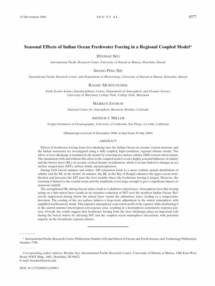
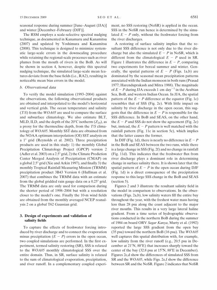
FIG. 1. Evaporation minus precipitation (E 2 P, cm day21) simulated from (top) SR and (bottom) the difference

SR 2 NoSR averaged in (left) JJA and (right) DJF for 1993–2004.


seasonal response during summer [June–August (JJA)]

and winter [December–February (DJF)].

The RSM employs a scale-selective spectral nudging

technique, as documented in Kanamaru and Kanamitsu

(2007) and updated by Yoshimura and Kanamitsu

(2008). This technique is designed to minimize system-

atic large-scale errors in the downscaling procedure

while retaining the regional-scale processes such as river

plumes from the mouth of rivers in the BoB. As will

be shown in section 4, however, despite this spectral

nudging technique, the simulated large-scale mean fea-

tures deviate from the base fields (i.e., RA2), resulting in

noticeable mean bias errors in the model.

b. Observational data

To verify the model simulation (1993–2004) against

the observations, the following observational products

are obtained and interpolated to the model’s horizontal

and vertical grids. The ocean temperature and salinity

(T/S) from the WOA05 are used to compare the surface

and subsurface climatology. We also estimate BLT,

MLD, ILD, and the depth of the 208C isotherm (Z20), as

a proxy for the thermocline depth, from the T/S clima-

tology of WOA05. Monthly SST data are obtained from

the NOAA optimum interpolation (OI) SST analysis on

a 18 grid (Reynolds et al. 2002). Three precipitation

products are used in this study: 1) the monthly Global

Precipitation Climatology Project (GPCP) version 2

(Adler et al. 2003) on a 2.58 grid, 2) the Climate Prediction

Center Merged Analysis of Precipitation (CMAP) on

a global 2.58 grid (Xie and Arkin 1997), and finally 3) the

monthly Tropical Rainfall Measuring Mission (TRMM)

precipitation product 3B43 Version 6 (Huffman et al.

2007) that combines the TRMM data with an estimate

from the global gridded rain gauge data on a 0.258 grid.

The TRMM data are only used for comparison during

the shorter period of 1998–2004 but with a resolution

closer to the model’s one. Finally the 10-m wind fields

are obtained from the monthly averaged NCEP reanal-

ysis 2 on a global T62 Gaussian grid.

3. Design of experiments and validation ofsalinity fields

To capture the effects of freshwater forcing intro-

duced by river discharge and to connect the evaporation

minus precipitation (E 2 P) errors in the open ocean,

two coupled simulations are performed. In the first ex-

periment, termed salinity restoring (SR), SSS is relaxed

to the WOA05 monthly climatological SSS over the

entire domain. Thus, in SR, surface salinity is relaxed

to the sum of climatological evaporation, precipitation,

and river runoff. In a complementary coupled experi-

ment, no SSS restoring (NoSR) is applied in the ocean.

SSS in the NoSR run hence is determined by the simu-

lated E 2 P only, without the freshwater forcing from

the river discharges.

A restoring of surface salinity implies that the re-

sultant SSS difference is not only due to the river dis-

charge but also the simulated E 2 P in NoSR, which is

different from the climatological E 2 P used in SR.

Figure 1 illustrates the difference in E 2 P, comparing

two experiments for boreal summer and winter. Gen-

erally, the spatial patterns of E 2 P (Figs. 1a,b) are

dominated by the seasonal mean precipitation patterns

associated with the Indian monsoon in both runs (Prasad

1977; Harenduprakash and Mitra 1988). The magnitude

of E 2 P during JJA exceeds 1 cm day21 in the Arabian

Sea, BoB, and western Indian Ocean. In JJA, the spatial

pattern of the E 2 P difference at the equator (Fig. 1c)

resembles that of SSS (Fig. 2e). With little impact on

salinity by river discharge in the open ocean, this sug-

gests that the difference in E 2 P is responsible for the

SSS difference. In BoB and SEAS, on the other hand,

the E 2 P and SSS do not show the agreement (Fig. 2e)

but, instead, the E 2 P pattern is well matched with the

rainfall pattern (Fig. 11c in section 5c), which implies

that the latter causes the former.

In DJF (Fig. 1d), there is nearly no difference in E 2 P

in the BoB and SEAS between the two runs, while there

is a large change in SSS (Fig. 2f) and no change in rainfall

(Fig. 11d). This indicates that the freshwater flux from

river discharge plays a dominant role in determining

change in surface salinity there. It is shown later that the

spatial pattern of E 2 P in the open ocean during DJF

(Fig. 1d) is a direct consequence of the precipitation

response to this large SSS change in the BoB and SEAS

(section 5).

Figures 2 and 3 illustrate the resultant salinity field in

the model in comparison to observations. In the obser-

vations (Figs. 2a,b), low salinity waters fill the entire bay

throughout the year, with the freshest water mass having

less than 28 psu along the coast adjacent to the major

river mouths. This results in a very large lateral haline

gradient. From a time series of hydrographic observa-

tions conducted in the northern BoB during the summer

of 1984 on board ORV Sagar Kanya, Murty et al. (1992)

reported the large SSS gradient from the open bay

(35 psu) toward the northern BoB (16 psu). The WOA05

well captures this spatial distribution with, for example,

low salinity from the river runoff (e.g., 20.5 psu in De-

cember at 218N, 888E) that increases sharply toward the

center of the bay (32.8 psu at 158N, 888E in December).

Figures 2c,d show the differences of simulated SSS from

SR and the WOA05, while Figs. 2e,f show the difference

between SR and the NoSR. Figure 2 indicates that NoSR


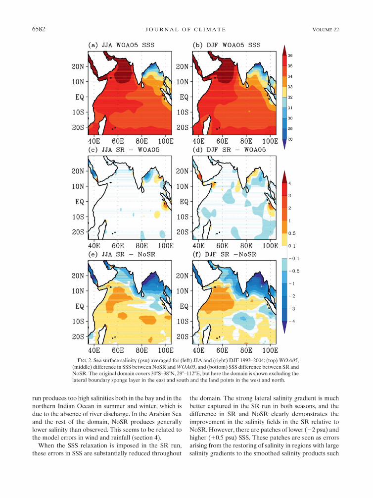
run produces too high salinities both in the bay and in the

northern Indian Ocean in summer and winter, which is

due to the absence of river discharge. In the Arabian Sea

and the rest of the domain, NoSR produces generally

lower salinity than observed. This seems to be related to

the model errors in wind and rainfall (section 4).

When the SSS relaxation is imposed in the SR run,

these errors in SSS are substantially reduced throughout

the domain. The strong lateral salinity gradient is much

better captured in the SR run in both seasons, and the

difference in SR and NoSR clearly demonstrates the

improvement in the salinity fields in the SR relative to

NoSR. However, there are patches of lower (22 psu) and

higher (10.5 psu) SSS. These patches are seen as errors

arising from the restoring of salinity in regions with large

salinity gradients to the smoothed salinity products such

FIG. 2. Sea surface salinity (psu) averaged for (left) JJA and (right) DJF 1993–2004: (top) WOA05,

(middle) difference in SSS between NoSR and WOA05, and (bottom) SSS difference between SR and

NoSR. The original domain covers 308S–388N, 298–1128E, but here the domain is shown excluding the

lateral boundary sponge layer in the east and south and the land points in the west and north.


as WOA05 (Yu and McCreary 2004). In such regions,

SSS restoring is particularly sensitive to the chosen relax-

ation time scale. We have chosen a strong relaxation (t 5

10 days), which, as is revealed in Fig. 2, reproduces the

spatial patterns of the observed salinity quite well but

can sometimes overshoot the SSS differences and switch

its sign in the regions of large salinity gradient.

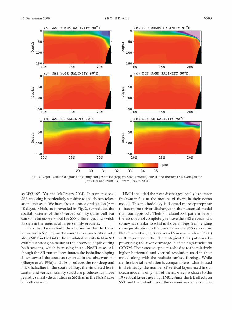
The subsurface salinity distribution in the BoB also

improves in SR. Figure 3 shows the transects of salinity

along 908E in the BoB. The simulated salinity field in SR

exhibits a strong halocline at the observed depth during

both seasons, which is missing in the NoSR case. Al-

though the SR run underestimates the isohaline sloping

down toward the coast as reported in the observations

(Shetye et al. 1996) and also produces the too-deep and

thick halocline in the south of Bay, the simulated hori-

zontal and vertical salinity structure produces far more

realistic salinity distribution in SR than in the NoSR case

in both seasons.

HM01 included the river discharges locally as surface

freshwater flux at the mouths of rivers in their ocean

model. This methodology is deemed more appropriate

to incorporate river discharges in the numerical model

than our approach. Their simulated SSS pattern never-

theless does not completely remove the SSS errors and is

somewhat similar to what is shown in Figs. 2e,f, lending

some justification to the use of a simple SSS relaxation.

Note that a study by Kurian and Vinayachandran (2007)

well reproduced the climatological SSS patterns by

prescribing the river discharge in their high-resolution

OCGM. Their success appears to be due to the relatively

higher horizontal and vertical resolution used in their

model along with the realistic surface forcings. While

our horizontal resolution is comparable to what is used

in their study, the number of vertical layers used in our

ocean model is only half of theirs, which is closer to the

19 vertical layers used by HM01. Since the BL effects on

SST and the definitions of the oceanic variables such as

FIG. 3. Depth–latitude diagrams of salinity along 908E for (top) WOA05, (middle) NoSR, and (bottom) SR averaged for

(left) JJA and (right) DJF from 1993 to 2004.


MLD and BL critically depend on vertical processes and

the resolutions of the model (Kara et al. 2000), we ex-

pect the results to be more similar to those from HM01,

if the river discharge were imposed locally.

In summary, despite the limitation of the experi-

mental setup, the comparison of E 2 P fluxes and SSS

indicate that the SSS relaxation method captures im-

portant aspects of Indian Ocean salinity variations rea-

sonably well (e.g., seasonal cycle) and, hence, is capable

of offering useful insights on the role of freshwater

oceanic forcing affecting the large-scale atmospheric

circulation.

4. Validation of model climatology

Before we investigate the sensitivity of the system to

surface freshening, this section discusses the seasonal

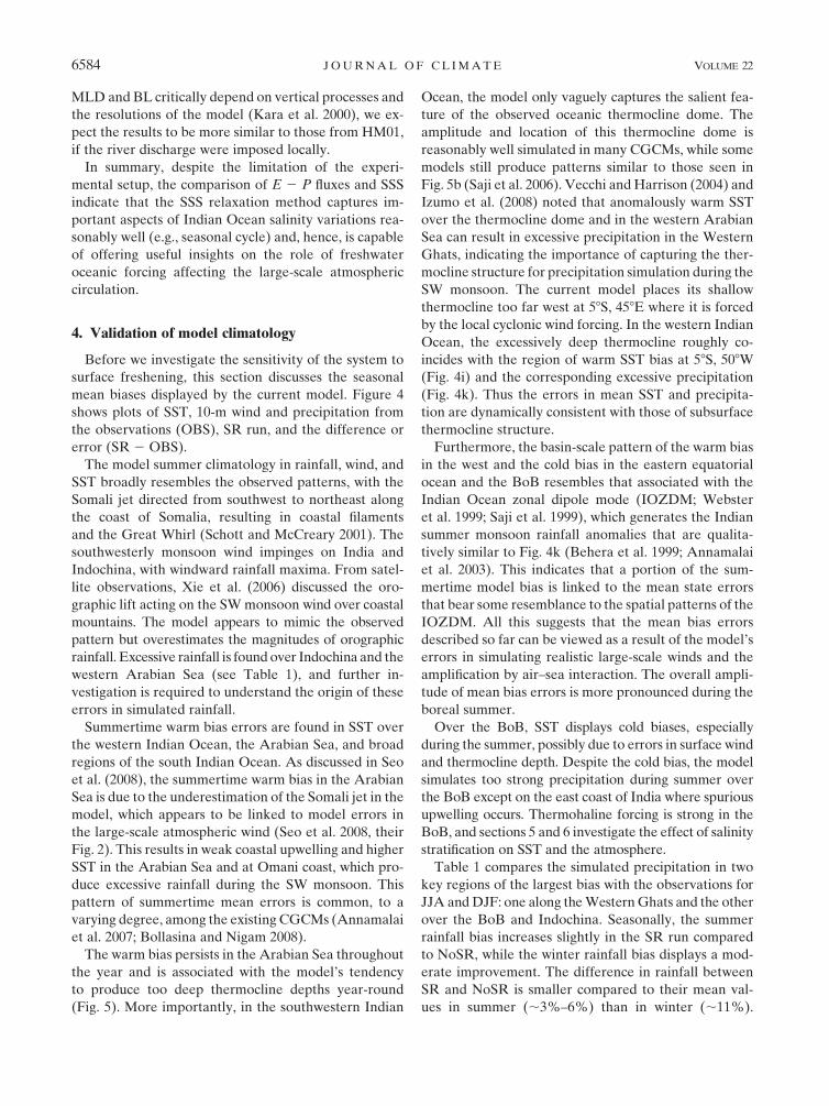
mean biases displayed by the current model. Figure 4

shows plots of SST, 10-m wind and precipitation from

the observations (OBS), SR run, and the difference or

error (SR 2 OBS).

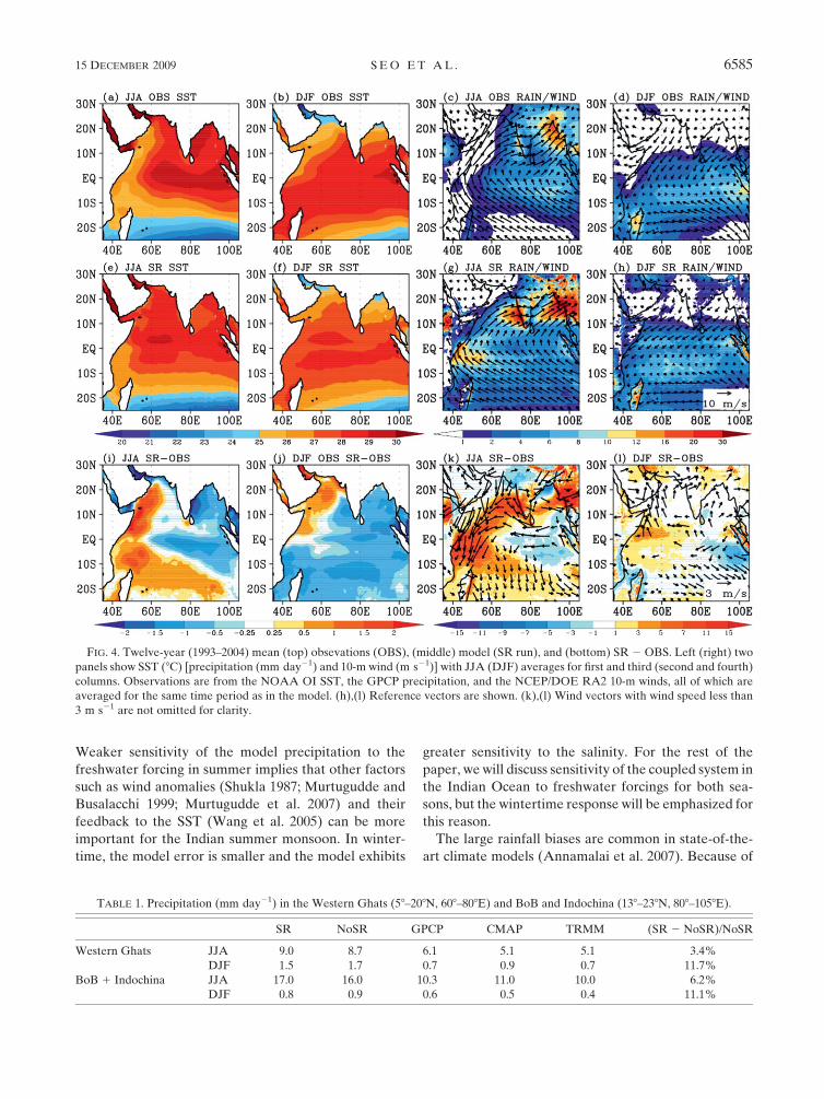
The model summer climatology in rainfall, wind, and

SST broadly resembles the observed patterns, with the

Somali jet directed from southwest to northeast along

the coast of Somalia, resulting in coastal filaments

and the Great Whirl (Schott and McCreary 2001). The

southwesterly monsoon wind impinges on India and

Indochina, with windward rainfall maxima. From satel-

lite observations, Xie et al. (2006) discussed the oro-

graphic lift acting on the SW monsoon wind over coastal

mountains. The model appears to mimic the observed

pattern but overestimates the magnitudes of orographic

rainfall. Excessive rainfall is found over Indochina and the

western Arabian Sea (see Table 1), and further in-

vestigation is required to understand the origin of these

errors in simulated rainfall.

Summertime warm bias errors are found in SST over

the western Indian Ocean, the Arabian Sea, and broad

regions of the south Indian Ocean. As discussed in Seo

et al. (2008), the summertime warm bias in the Arabian

Sea is due to the underestimation of the Somali jet in the

model, which appears to be linked to model errors in

the large-scale atmospheric wind (Seo et al. 2008, their

Fig. 2). This results in weak coastal upwelling and higher

SST in the Arabian Sea and at Omani coast, which pro-

duce excessive rainfall during the SW monsoon. This

pattern of summertime mean errors is common, to a

varying degree, among the existing CGCMs (Annamalai

et al. 2007; Bollasina and Nigam 2008).

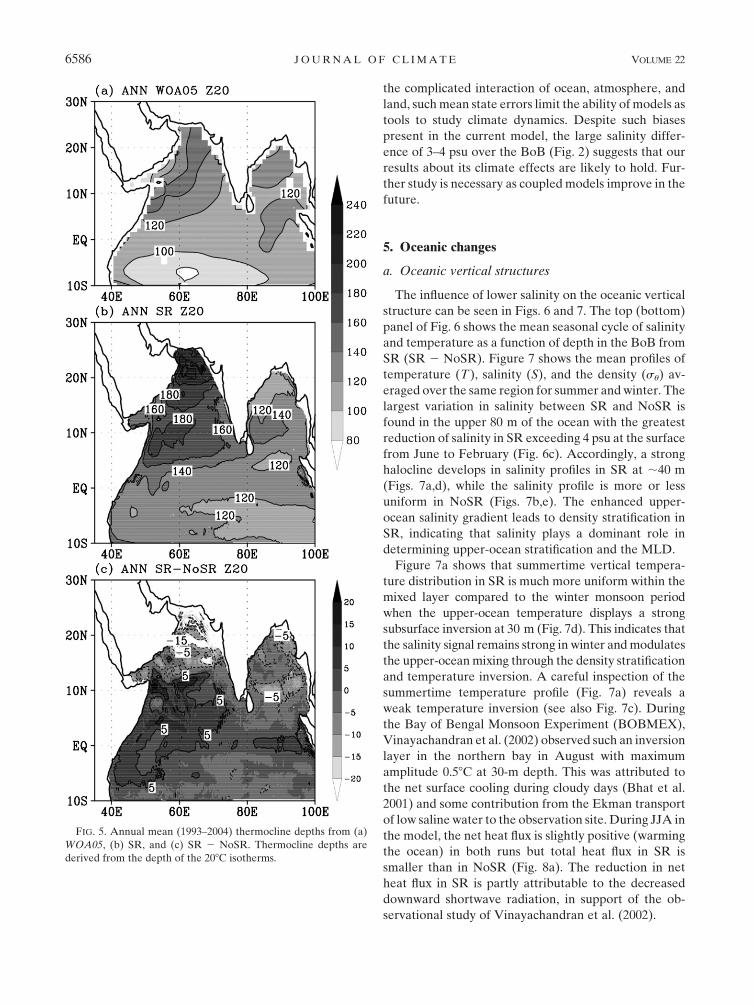
The warm bias persists in the Arabian Sea throughout

the year and is associated with the model’s tendency

to produce too deep thermocline depths year-round

(Fig. 5). More importantly, in the southwestern Indian

Ocean, the model only vaguely captures the salient fea-

ture of the observed oceanic thermocline dome. The

amplitude and location of this thermocline dome is

reasonably well simulated in many CGCMs, while some

models still produce patterns similar to those seen in

Fig. 5b (Saji et al. 2006). Vecchi and Harrison (2004) and

Izumo et al. (2008) noted that anomalously warm SST

over the thermocline dome and in the western Arabian

Sea can result in excessive precipitation in the Western

Ghats, indicating the importance of capturing the ther-

mocline structure for precipitation simulation during the

SW monsoon. The current model places its shallow

thermocline too far west at 58S, 458E where it is forced

by the local cyclonic wind forcing. In the western Indian

Ocean, the excessively deep thermocline roughly co-

incides with the region of warm SST bias at 58S, 508W

(Fig. 4i) and the corresponding excessive precipitation

(Fig. 4k). Thus the errors in mean SST and precipita-

tion are dynamically consistent with those of subsurface

thermocline structure.

Furthermore, the basin-scale pattern of the warm bias

in the west and the cold bias in the eastern equatorial

ocean and the BoB resembles that associated with the

Indian Ocean zonal dipole mode (IOZDM; Webster

et al. 1999; Saji et al. 1999), which generates the Indian

summer monsoon rainfall anomalies that are qualita-

tively similar to Fig. 4k (Behera et al. 1999; Annamalai

et al. 2003). This indicates that a portion of the sum-

mertime model bias is linked to the mean state errors

that bear some resemblance to the spatial patterns of the

IOZDM. All this suggests that the mean bias errors

described so far can be viewed as a result of the model’s

errors in simulating realistic large-scale winds and the

amplification by air–sea interaction. The overall ampli-

tude of mean bias errors is more pronounced during the

boreal summer.

Over the BoB, SST displays cold biases, especially

during the summer, possibly due to errors in surface wind

and thermocline depth. Despite the cold bias, the model

simulates too strong precipitation during summer over

the BoB except on the east coast of India where spurious

upwelling occurs. Thermohaline forcing is strong in the

BoB, and sections 5 and 6 investigate the effect of salinity

stratification on SST and the atmosphere.

Table 1 compares the simulated precipitation in two

key regions of the largest bias with the observations for

JJA and DJF: one along the Western Ghats and the other

over the BoB and Indochina. Seasonally, the summer

rainfall bias increases slightly in the SR run compared

to NoSR, while the winter rainfall bias displays a mod-

erate improvement. The difference in rainfall between

SR and NoSR is smaller compared to their mean val-

ues in summer (;3%–6%) than in winter (;11%).


Weaker sensitivity of the model precipitation to the

freshwater forcing in summer implies that other factors

such as wind anomalies (Shukla 1987; Murtugudde and

Busalacchi 1999; Murtugudde et al. 2007) and their

feedback to the SST (Wang et al. 2005) can be more

important for the Indian summer monsoon. In winter-

time, the model error is smaller and the model exhibits

greater sensitivity to the salinity. For the rest of the

paper, we will discuss sensitivity of the coupled system in

the Indian Ocean to freshwater forcings for both sea-

sons, but the wintertime response will be emphasized for

this reason.

The large rainfall biases are common in state-of-the-

art climate models (Annamalai et al. 2007). Because of

TABLE 1. Precipitation (mm day21) in the Western Ghats (58–208N, 608–808E) and BoB and Indochina (138–238N, 808–1058E).

SR NoSR GPCP CMAP TRMM (SR 2 NoSR)/NoSR

Western Ghats JJA 9.0 8.7 6.1 5.1 5.1 3.4%

DJF 1.5 1.7 0.7 0.9 0.7 11.7%

BoB 1 Indochina JJA 17.0 16.0 10.3 11.0 10.0 6.2%

DJF 0.8 0.9 0.6 0.5 0.4 11.1%

FIG. 4. Twelve-year (1993–2004) mean (top) obsevations (OBS), (middle) model (SR run), and (bottom) SR 2 OBS. Left (right) two

panels show SST (8C) [precipitation (mm day21) and 10-m wind (m s21)] with JJA (DJF) averages for first and third (second and fourth)

columns. Observations are from the NOAA OI SST, the GPCP precipitation, and the NCEP/DOE RA2 10-m winds, all of which are

averaged for the same time period as in the model. (h),(l) Reference vectors are shown. (k),(l) Wind vectors with wind speed less than

3 m s21 are not omitted for clarity.


the complicated interaction of ocean, atmosphere, and

land, such mean state errors limit the ability of models as

tools to study climate dynamics. Despite such biases

present in the current model, the large salinity differ-

ence of 3–4 psu over the BoB (Fig. 2) suggests that our

results about its climate effects are likely to hold. Fur-

ther study is necessary as coupled models improve in the

future.

5. Oceanic changes

a. Oceanic vertical structures

The influence of lower salinity on the oceanic vertical

structure can be seen in Figs. 6 and 7. The top (bottom)

panel of Fig. 6 shows the mean seasonal cycle of salinity

and temperature as a function of depth in the BoB from

SR (SR 2 NoSR). Figure 7 shows the mean profiles of

temperature (T), salinity (S), and the density (su) av-

eraged over the same region for summer and winter. The

largest variation in salinity between SR and NoSR is

found in the upper 80 m of the ocean with the greatest

reduction of salinity in SR exceeding 4 psu at the surface

from June to February (Fig. 6c). Accordingly, a strong

halocline develops in salinity profiles in SR at ;40 m

(Figs. 7a,d), while the salinity profile is more or less

uniform in NoSR (Figs. 7b,e). The enhanced upper-

ocean salinity gradient leads to density stratification in

SR, indicating that salinity plays a dominant role in

determining upper-ocean stratification and the MLD.

Figure 7a shows that summertime vertical tempera-

ture distribution in SR is much more uniform within the

mixed layer compared to the winter monsoon period

when the upper-ocean temperature displays a strong

subsurface inversion at 30 m (Fig. 7d). This indicates that

the salinity signal remains strong in winter and modulates

the upper-ocean mixing through the density stratification

and temperature inversion. A careful inspection of the

summertime temperature profile (Fig. 7a) reveals a

weak temperature inversion (see also Fig. 7c). During

the Bay of Bengal Monsoon Experiment (BOBMEX),

Vinayachandran et al. (2002) observed such an inversion

layer in the northern bay in August with maximum

amplitude 0.58C at 30-m depth. This was attributed to

the net surface cooling during cloudy days (Bhat et al.

2001) and some contribution from the Ekman transport

of low saline water to the observation site. During JJA in

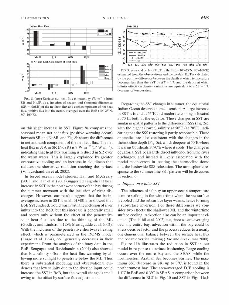
the model, the net heat flux is slightly positive (warming

the ocean) in both runs but total heat flux in SR is

smaller than in NoSR (Fig. 8a). The reduction in net

heat flux in SR is partly attributable to the decreased

downward shortwave radiation, in support of the ob-

servational study of Vinayachandran et al. (2002).

FIG. 5. Annual mean (1993–2004) thermocline depths from (a)

WOA05, (b) SR, and (c) SR 2 NoSR. Thermocline depths are

derived from the depth of the 208C isotherms.


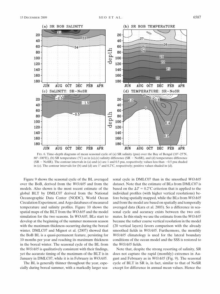
Figure 9 shows the seasonal cycle of the BL averaged

over the BoB, derived from the WOA05 and from the

models. Also shown is the most recent estimate of the

global BLT by DMLC07 derived from the National

Oceanographic Data Center (NODC), World Ocean

Circulation Experiment, and Argo databases of measured

temperature and salinity profiles. Figure 10 shows the

spatial maps of the BLT from the WOA05 and the model

simulation for the two seasons. In WOA05, BLs start to

develop at the beginning of the summer monsoon season

with the maximum thickness occurring during the boreal

winter. DMLC07 and Mignot et al. (2007) showed that

the BoB BL is a quasi-permanent feature, persisting for

10 months per year and reaching its maximum thickness

in the boreal winter. The seasonal cycle of the BL from

the WOA05 is qualitatively consistent with their findings,

yet the accurate timing of the maximum of the BLT is in

January in DMLC07, while it is in February in WOA05.

The BL is generally thinner throughout the year, espe-

cially during boreal summer, with a markedly larger sea-

sonal cycle in DMLC07 than in the smoothed WOA05

dataset. Note that the estimate of BLs from DMLC07 is

based on the DT 5 0.28C criterion that is applied to the

individual profiles (with higher vertical resolutions) be-

fore being spatially mapped, while the BLs from WOA05

and from the model are based on spatially and temporally

averaged data (Kara et al. 2003). So a difference in sea-

sonal cycle and accuracy exists between the two esti-

mates. In this study we use the estimate from the WOA05

because the rather coarse vertical resolution in the model

(20 vertical layers) favors comparison with the already

smoothed fields in WOA05. Furthermore, the monthly

WOA05 climatology is used for the lateral boundary

conditions of the ocean model and the SSS is restored to

the WOA05 fields.

Note that, despite the strong resorting of salinity, SR

does not capture the rapid (monthly) extremes in Au-

gust and February as in WOA05 (Fig. 9). The seasonal

cycle of BLT in SR is, in fact, similar to that of NoSR

except for difference in annual mean values. Hence the

FIG. 6. Time–depth diagrams of mean seasonal cycle of (a) SR salinity (psu) over the Bay of Bengal (108–258N,

808–1008E), (b) SR temperature (8C) as in (a),(c) salinity difference (SR 2 NoSR), and (d) temperature difference

(SR 2 NoSR). The contour intervals in (a) and (c) are 1 and 0.5 psu, respectively; values less than 20.5 psu shaded

in (c). The contour intervals for (b) and (d) are 18 and 0.28C, respectively; positive values shaded in (d).


effect of restoring surface salinity appears to have the

largest impact on the year-mean values of BLT, while its

seasonal cycle is dominated by model climatology.

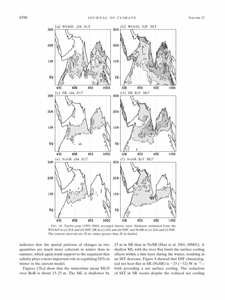
In JJA, WOA05 shows a 40–50-m thick BL along

the coast of the bay, with maximum thickness of 50–

60 m along the eastern coast (Fig. 10a). In DJF, the

BLT reaches 70 m in the northern bay and the SEAS

(Fig. 10b). The SR run qualitatively captures key as-

pects of these spatial patterns. Specifically, the 20–40-m

thickness of the BL in the BoB and Arabian Sea in JJA

and the thick BL centered in the BoB and SEAS in DJF

are evident. However, the BLT in SR is generally un-

derestimated throughout the domain compared to the

WOA05 and some features of the BL in the eastern

equatorial ocean are not reproduced. In particular, the

BLT in the SEAS during DJF is thicker and spatially

more extensive toward the Arabian Sea in SR than in

WOA05. Note, however, that the NoSR run essentially

fails to reproduce the important features of the BL in the

Indian Ocean, including the spatial distribution and its

seasonal cycle.

b. Impact on summer SST

Modulation of vertical stratification by salinity and the

BL has an important effect on the ML temperature and

SST. Figure 11a illustrates the spatial patterns of these

changes in SST during JJA season. A local increase in

SST can be found along the northwestern coast of the bay

adjacent to the mouths of the major rivers, which warm

up to 0.48C with the inclusion of river runoff. However,

the areal extents of this increase in SST are limited to the

coastal boundaries and hence, when averaged over the

entire Bay, the increase in SST is rather small, 0.18C in

this model. This is clearly not sufficient to offset the cold

bias shown in Fig. 4i and implies that the effect of river

input on SST is weak during summer and the cold bias in

the model is more closely related to wind anomalies, as

discussed in section 4.

Since the isothermal layer is deep and the net surface

heat flux is weak over the summer BoB, the warming

effect due to the weakened mixing is not pronounced.

Furthermore, the surface heat flux acts as a damping

FIG. 7. (top) JJA and (bottom) DJF mean profiles of salinity (S 2 10 psu), temperature (T, 8C), and density (su)

averaged over Bay of Bengal (108–258N, 808–1008E) from (a) SR, (b) NoSR, and (c) SR 2 NoSR. The quantities are

averaged for 12 years (1993–2004). There are approximately 14 vertical layers in the upper 200 m (1.9, 5.7, 9.7, 14.0,

18.9, 24.7, 31.6, 40.1, 50.9, 64.9, 83.3, 107.7, 140.6, and 185.1 m).


on this slight increase in SST. Figure 8a compares the

seasonal mean net heat flux (positive warming ocean)

between SR and NoSR, and Fig. 8b shows the difference

in net and each component of the net heat flux. The net

heat flux in JJA in SR (NoSR) is 9 W m22 (17 W m22),

indicating that heat flux warming is reduced in SR over

the warm water. This is largely explained by greater

evaporative cooling and an increase in cloudiness that

reduces the shortwave radiation reaching the surface

(Vinayachandran et al. 2002).

In forced ocean model studies, Han and McCreary

(2001) and Han et al. (2001) suggested a significant local

increase in SST in the northwest corner of the bay during

the summer monsoon with the inclusion of river dis-

charges. However, our results suggest that the basin-

average increase in SST is small. HM01 also showed that

BoB SST, indeed, would warm with the inclusion of river

influx into the BoB, but this increase is generally small

and occurs only without the effect of the penetrative

solar heat flux loss due to the thinning of the ML

(Godfrey and Lindstrom 1989; Murtugudde et al. 2002).

With the inclusion of the penetrative shortwave heating

effect, which is parameterized in the ROMS model

(Large et al. 1994), SST generally decreases in their

experiment. From the analysis of the buoy data in the

BoB, Sengupta and Ravichandran (2001) also showed

that low salinity offsets the heat flux warming by al-

lowing more sunlight to penetrate below the ML. Thus

there is substantial modeling and observational evi-

dences that low salinity due to the riverine input could

increase the SST in BoB, but the overall change is small

owing to the offset by surface flux adjustments.

Regarding the SST changes in summer, the equatorial

Indian Ocean deserves some attention. A large increase

in SST is found at 558E and moderate cooling is located

at 708E, both at the equator. These changes in SST are

similar in spatial patterns to the difference in SSS (Fig. 2e),

with the higher (lower) salinity at 508E (at 708E), indi-

cating that the SSS restoring is partly responsible. These

anomalies are also consistent with the changes in the

thermocline depth (Fig. 5c), which deepens at 508E where

it warms but shoals at 708E where it cools. The change in

equatorial SST bears little direct influence from the river

discharges, and instead is likely associated with the

model mean errors in locating the thermocline dome

and the basinwide SSS relaxation. The atmospheric re-

sponse to the summertime SST pattern will be discussed

in section 6.

c. Impact on winter SST

The influence of salinity on upper-ocean temperature

is more striking in the wintertime when the sea surface

is cooled and the subsurface layer warms, hence forming

a subsurface inversion. For these differences we con-

sider two effects: the shallower ML and the wintertime

surface cooling. Advection also can be an important el-

ement (Thadathil et al. 2002) but, since we are averaging

over the entire bay, advection within the bay could be

a less decisive factor and the process reduces to a nearly

one-dimensional balance between the surface heat flux

and oceanic vertical mixing (Rao and Sivakumar 2000).

Figure 11b illustrates the reduction in SST in our

model in response to surface freshening. Large cooling

occurs over the entire bay and the SEAS, while the

northwestern Arabian Sea becomes warmer. The max-

imum SST decrease in SR, up to 38C, is found in the

northernmost bay. The area-averaged DJF cooling is

1.18C in BoB and 0.38C in SEAS. A comparison between

the difference in BLT in Fig. 10 and SST in Figs. 11a,b

FIG. 8. (top) Surface net heat flux climatology (W m22) from

SR and NoSR as a function of season and (bottom) difference

(SR 2 NoSR) of the net heat flux and each component of net heat

flux, positive flux into the ocean, averaged over the BoB (108–258N,

808–1008E).

FIG. 9. Seasonal cycle of BLT in the BoB (108–258N, 808–1008E)

estimated from the observations and the models. BLT is calculated

by the positive difference between the depth at which temperature

becomes less than the SST by DT 5 18C and the depth at which

salinity effects on density variations are equivalent to a DT 5 18C

decrease of temperature.


indicates that the spatial patterns of changes in two

quantities are much more coherent in winter than in

summer, which again lends support to the argument that

salinity plays a more important role in regulating SSTs in

winter in the current model.

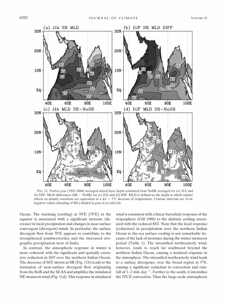
Figures 12b,d show that the wintertime mean MLD

over BoB is about 15–25 m. The ML is shallower by

25 m in SR than in NoSR (Han et al. 2001; HM01). A

shallow ML with the river flux limits the surface cooling

effects within a thin layer during the winter, resulting in

an SST decrease. Figure 8 showed that DJF climatolog-

ical net heat flux in SR (NoSR) is 225 (252) W m22—

both providing a net surface cooling. The reduction

of SST in SR occurs despite the reduced net cooling

FIG. 10. Twelve-year (1993–2004) averaged barrier layer thickness estimated from the

WOA05 in (a) JJA and (b) DJF, SR in (c) JJA and (d) DJF, and NoSR in (e) JJA and (f) DJF.

The contour intervals are 20 m; values greater than 20 m shaded.


(by reduced evaporative cooling over the cold water),

demonstrating that it is an oceanic process that causes

the SST cooling.

6. Atmospheric response to SST changes

The previous section showed that lowering salinity

via SSS relaxation induces small changes in local SST

(where added freshwater forcing is large) during the

summer, but in winter it leads to a striking basinwide

cooling that is spatially coherent with the change in SSS

and the BL. The simulated changes in surface winds and

rainfall also exhibit a spatial structure more coherent with

the underlying SST in winter than in summer. This section

discusses the atmospheric response to the change in SST.

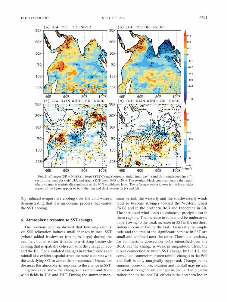
Figures 11c,d show the changes in rainfall and 10-m

wind fields in JJA and DJF. During the summer mon-

soon period, the westerly and the southwesterly winds

tend to become stronger toward the Western Ghats

(WG) and in the northern BoB and Indochina in SR.

The increased wind leads to enhanced precipitation in

these regions. The increase in rain could be understood

in part owing to the weak increase in SST in the northern

Indian Ocean including the BoB. Generally the ampli-

tude and the area of the significant increase in SST are

small and confined near the coast. There is a tendency

for summertime convection to be intensified over the

BoB, but the change is weak in magnitude. Thus, the

direct connection between SST change by the BL and

consequent summer monsoon rainfall changes in the WG

and BoB is only marginally supported. Change in the

summer monsoon precipitation and rainfall may instead

be related to significant changes in SST at the equator

rather than to the local BL effects in the northern Indian

FIG. 11. Changes (SR 2 NoSR) in (top) SST (8C) and (bottom) rainfall (mm day21) and 10-m wind speed (m s21),

vectors averaged for (left) JJA and (right) DJF from 1993 to 2004. The overlaid black contours denote the region

where change is statistically significant at the 90% confidence level. The reference vector shown in the lower-right

corner of the figure applies to both the thin and thick vectors in (c) and (d).


Ocean. The warming (cooling) at 508E (708E) at the

equator is associated with a significant increase (de-

crease) in local precipitation and changes in near-surface

convergent (divergent) winds. In particular, the surface

divergent flow from 708E appears to contribute to the

strengthened southwesterlies and the increased oro-

graphic precipitation west of India.

In contrast, the atmospheric response in winter is

more coherent with the significant and spatially exten-

sive reduction in SST over the northern Indian Ocean.

The decrease of SST shown in SR (Fig. 11b) leads to the

formation of near-surface divergent flow originating

from the BoB and the SEAS and amplifies the simulated

NE monsoon wind (Fig. 11d). This response in simulated

wind is consistent with a linear baroclinic response of the

troposphere (Gill 1980) to the diabatic cooling associ-

ated with the reduced SST. Note that the local response

(reduction) in precipitation over the northern Indian

Ocean to the sea surface cooling is not remarkable be-

cause of the lack of moisture during the winter monsoon

period (Table 1). The intensified northeasterly wind,

however, tends to reach far southward beyond the

northern Indian Ocean, causing a nonlocal response in

the atmosphere. The intensified northeasterly wind leads

to a surface divergence over the broad region at 58N,

causing a significant reduction in convection and rain-

fall of 1–2 mm day21. Farther to the south, it intensifies

the ITCZ convection. Thus the large-scale atmospheric

FIG. 12. Twelve-year (1993–2004) averaged mixed layer depth estimated from NoSR averaged for (a) JJA and

(b) DJF. MLD differences (SR 2 NoSR) for (c) JJA and (d) DJF. MLD is defined as the depth at which salinity

effects on density variations are equivalent to a DT 5 18C decrease of temperature. Contour intervals are 10 m;

negative values (shoaling of ML) shaded in gray in (c) and (d).


response to the changes in SST due to the BL is to dis-

place the ITCZ southward.

Note that CGCMs typically have large BL biases in

the BoB and the northern Indian Ocean. In particular, in

the latest Community Climate System Model (version

3.5) the BL is rather weak (J. Mignot 2008, personal

communication), and in DJF there is too much pre-

cipitation north and near the equator and too little south

of the equator at 108–158S (Jochum and Potemra 2008).

This suggests that in current GCMs the weak BL phys-

ics, among other factors, could be partially responsible

for the tropical precipitation biases. By analyzing the

BLs in several CGCMs, Breugem et al. (2008) hypoth-

esized a positive BL–SST–ITCZ feedback that main-

tains model warm and fresh biases in the southeastern

equatorial Atlantic Ocean. Within their feedback pro-

cess, the BL is an active and dynamic impetus for gen-

erating climate anomalies. The results from previous

and present studies suggest that it is critical to capture

realistic BLs in coupled climate models for improving

the simulation and prediction of regional climate vari-

ability, including the Indian monsoons.

7. Summary and discussion

We have used a high-resolution, regional coupled

ocean–atmosphere model to investigate the effect of

river water on the seasonal cycle in the Indian Ocean

climate. The model mean state exhibits deviations from

observations, with biases in thermocline depth, SST,

wind, and rainfall. These biases are somewhat similar

in magnitude and spatial pattern to those in current

CGCMs over the same area [see reviews of the monsoon

biases in the Intergovernmental Panel on Climate Change

coupled GCMs by Annamalai et al. 2007 and Bollasina

and Nigam 2008].

Our initial hypothesis that motivated this study is that

the introduction of a freshwater cap in the Bay of Bengal

(BoB) would alleviate the summertime cold bias present

in the model through the influence of the barrier layer

(BL) on mixing SST. To our surprise, there is no signif-

icant change in summertime SST in the northern Indian

Ocean despite a more realistic oceanic vertical structure

due to the freshwater forcing. There is no significant di-

rect response in wind and rainfall during the southwest

(SW) monsoon period to the local change in SST over

the BoB. However, we find a significant influence of the

BL on local SST during boreal winter with a large atmo-

spheric response in the northeast (NE) monsoon.

The main results are summarized as follows: During

the SW monsoon period, a large freshwater influx from

rivers, modeled here via SSS relaxation, generates a

strong halocline in the BoB, leading to the formation of

BLs and suppressing the mixing between surface and

subsurface water. With a reduced warming by surface

heat flux and the persistent subsurface warming from

the previous winter, the summertime temperature pro-

file exhibits a weak inversion as well. Because of the

deep isothermal layer, the weakened mixing effect is

not sufficient to further raise the SSTs. Overall, the

increase in summer SST averaged over the bay is 0.18C

(not significant at the 90% level), except for the coastal

regions adjacent to the mouths of major rivers where

SST warms up to 0.48C. This is qualitatively consistent

with the finding from Han et al. (2001) and HM01 who

reported greater warming of 0.58–1.08C. The SST warm-

ing in SR occurs despite the enhanced damping by the

evaporative cooling effect and the reduced shortwave

radiation flux, indicating that greater warming in forced

ocean models underestimates negative atmospheric

damping.

The SW monsoon wind somewhat strengthens in the

Western Ghats and northern BoB, causing a rainfall

increase in the northern Indian Ocean. The insignificant

increase in SST in the northern Indian Ocean does not

appear to be responsible for the stronger wind and

rainfall. Instead, the divergent flows in the equatorial

Indian Ocean, in response to changes in SST there, ap-

pear to exert the greater atmospheric influence over the

northern Indian Ocean.

During the winter monsoon season, the BLT attains

its maximum in the BoB, and the mixed layer conse-

quently becomes shallower. The vertical trapping of the

wintertime cooling efficiently decrease the SST by an

average of 1.18C. The SR run exhibits a strong sub-

surface inversion layer in the BoB (and southeast Ara-

bian Sea, as discussed by Thadathil and Gosh 1992) with

amplitudes of 0.88C (Figs. 6 and 7), consistent with ob-

servations. Wintertime cooling of SST in the BoB results

in nearly no changes in local rainfall and convection

because of lack of moisture convection and the cold SST.

Instead, the reduced SST in the northern Indian Ocean

amplifies the NE monsoon winds through a linear baro-

clinic response in the atmosphere. This results in a sig-

nificant reduction of convection and rainfall around at

58N while enhancing it south of the equator. This in-

dicates a possible connection of ocean stratification with

the large-scale atmospheric dynamics during the NE

monsoon period.

Masson et al. (2005) suggested from a CGCM exper-

iment that there is a link between the spatial structure of

the salinity in the SEAS and the onset of the summer

monsoon. This led them to hypothesize that the spatial

extent of the BL during the premonsoon season could be

a useful predictor of the onset of the summer monsoon.

Our model results differ in that the BL had no significant


impact on summer SST and the SW monsoon. Instead

we find that the BL in the BoB leaves its clear signature

on the wintertime SST and subsequently induces large-

scale adjustments in convection and rainfall across the

equator during the winter monsoon. The importance of

understanding the BL dynamics in the BoB in winter is

further supported by the fact that the simulated mon-

soon response is not limited to the BoB but extends to

the ITCZ and far into the Southern Hemisphere.

Further studies are necessary to determine the de-

tailed structure of this remote atmospheric response and

assess its potential impacts on climate. There is a clear

need for efforts in understanding the performances of

coupled GCMs in reproducing the observed BLs (Kara

et al. 2003; DMLC07) in the Indian Ocean. The results

of Breugem et al. (2008) in the Atlantic suggest that

errors in the BL can cause climate biases through mul-

tiple feedback processes in coupled climate models (Lin

2007). A better assessment of the impact of BLs on cli-

mate requires an intercomparison exercise using the

results from those climate models with and without the

salinity and BL effects. These kinds of studies will help

determine the extent to which common biases in the

climate models can be attributed to BL errors. It will

also help detect common and robust features of the

sensitivity of the regional climate system to the BLs.

Such research will greatly improve our understanding on

the potential role of the salinity and the BL in large-scale

climate variability, including the Indian monsoon.

Acknowledgments. HS acknowledges the NOAA Cli-

mate and Global Change Postdoctoral Fellowship Pro-

gram, administered by the University Corporation for

atmospheric Research. SPX thanks support from the

NSF and Japan Agency for Marine-Earth Science and

Technology. We thank three anonymous reviewers for

their comments and suggestions, which substantially im-

proved the quality of the manuscript. We acknowledge

the Center for Observations, Modeling and Prediction

at Scripps (COMPAS) for providing the required com-

puter resources for the coupled model simulation. HS

thanks M. Kanamitsu, K. Yoshimura, N. Schneider,

H. Annamalai, and Z. Yu for their stimulating discussions

and comments. NCEP Reanalysis 2 data and NOAA OI

SST analysis were provided by the NOAA/OAR/ESRL

PSD, Boulder, Colorado, from their Web site at http://

www.cdc.noaa.gov. The GPCP and the CMAP pre-

cipitation data were obtained from NCAR Climate Anal-

ysis Section Data Catalog at http://www.cgd.ucar.edu/cas/

catalog. The TRMM 3B43_V6 rainfall data were ob-

tained from http://disc.sci.gsfc.nasa.gov. The global MLD/

BLT climatology dataset was provided from http://www.

locean-ipsl.upmc.fr/;cdblod.

REFERENCES

Adler, R. F., and Coauthors, 2003: The Version-2 Global Pre-

cipitation Climatology Project (GPCP) monthly precipitation

analysis (1979–present). J. Hydrometeor., 4, 1147–1167.

Annamalai, H., R. Murtugudde, J. Potemra, S. P. Xie, P. Liu, and

B. Wang, 2003: Coupled dynamics over the Indian Ocean: Spring

initiation of the zonal mode. Deep-Sea Res. II, 50, 2305–2330.

——, K. Hamilton, and K. R. Sperber, 2007: South Asian summer

monsoon and its relationship with ENSO in the IPCC AR4

simulations. J. Climate, 20, 1071–1092.

Antonov, J. I., R. A. Locarnini, T. P. Boyer, A. V. Mishonov, and

H. E. Garcia, 2006: Salinity. Vol. 2, World Ocean Atlas 2005,

NOAA Atlas NESDIS 62, 182 pp.

Behera, S. K., R. Krishnan, and T. Yamagata, 1999: Unusual

ocean–atmosphere conditions in the tropical Indian Ocean

during 1994. Geophys. Res. Lett., 26, 3001–3004.

Bhat, G. S., and Coauthors, 2001: BOBMEX: The Bay of Bengal

Monsoon Experiment. Bull. Amer. Meteor. Soc., 82, 2217–2243.

Bollasina, M., and S. Nigam, 2008: Indian Ocean SST, evaporation,

and precipitation during the South Asian summer monsoon

in IPCC-AR4 coupled simulations. Climate Dyn., doi:10.1007/

s00382-008-0477-4.

Breugem, W.-P., P. Chang, C. J. Jang, J. Mignot, and W. Hazeleger,

2008: Barrier layers and tropical Atlantic SST biases in cou-

pled GCMs. Tellus, 60, 885–897.

da Silva, A. M., C. Young-Molling, and S. Levitus, 1994: Atlas of

surface marine data 1994. NOAA Atlas NESDIS 6-110, 83 pp.

de Boyer Montegut, C., J. Mignot, A. Lazar, and S. Cravatte, 2007:

Control of salinity on the mixed layer depth in the world

ocean: 1. General description. J. Geophys. Res., 112, C06011,

doi:10.1029/2006JC003953.

Durand, F., S. R. Shetye, J. Vialard, D. Shankar, S. S. C. Shenoi,

C. Ethe, and G. Madec, 2004: Impact of temperature in-

versions on SST evolution in the southeastern Arabian Sea

during the pre-summer monsoon season. Geophys. Res. Lett.,

31, L01305, doi:10.1029/2003GL018906.

Gadgil, S., P. V. Joseph, and N. V. Joshi, 1984: Ocean-atmosphere

coupling over monsoon regions. Nature, 312, 141–143.

Gill, A., 1980: Some simple solutions for heat-induced tropical

circulation. Quart. J. Roy. Meteor. Soc., 106, 447–462.

Godfrey, J. S., and E. J. Lindstrom, 1989: The heat budget of the

equatorial west Pacific surface mixed layer. J. Geophys. Res.,

94 (C6), 8007–8017.

Haidvogel, D. B., H. G. Arango, K. Hedstrom, A. Beckmann,

P. Malanotte-Rizzoli, and A. F. Shchepetkin, 2000: Model

evaluation experiments in the North Atlantic Basin: Simula-

tions in nonlinear terrain-following coordinates. Dyn. Atmos.

Oceans, 32, 239–281.

Han, W., and J. P. McCreary Jr., 2001: Modeling salinity distribu-

tions in the Indian Ocean. J. Geophys. Res., 106 (C1), 859–878.

——, ——, and K. E. Kohler, 2001: Influence of precipitation minus

evaporation and Bay of Bengal rivers on dynamics, thermo-

dynamics, and mixed layer physics in the upper Indian Ocean.

J. Geophys. Res., 106 (C4), 6895–6916.

Harenduprakash, L. L., and A. K. Mitra, 1988: Vertical turbulent

mass flux below the sea surface and air-sea interaction: Monsoon

region of the Indian Ocean. Deep-Sea Res. I, 43, 1423–1451.

Hastenrath, S., and P. J. Lamb, 1979: The Oceanic Heat Budget.

Vol. 2, Climatic Atlas of the Indian Ocean, University of

Wisconsin Press, 110 pp.

Howden, S. D., and R. Murtugudde, 2001: Effects of river inputs into

the Bay of Bengal. J. Geophys. Res., 106 (C9), 19 825–19 843.


Huffman, G. J., and Coauthors, 2007: The TRMM Multisatellite

Precipitation Analysis (TMPA): Quasi-global, multiyear,

combined-sensor precipitation estimates at fine scale. J. Hy-

drometeor., 8, 38–55.

Izumo, T., C. de Boyer Montegut, J. J. Luo, S. K. Behera,

S. Masson, and T. Yamagata, 2008: The role of the western

Arabian Sea upwelling in Indian monsoon rainfall variability.

J. Climate, 21, 5603–5623.

Jochum, M., and J. T. Potemra, 2008: Sensitivity of tropical rainfall

to Banda Sea diffusivity in the Community Climate System

Model. J. Climate, 21, 6445–6454.

Joseph, P. V., 1990: Monsoon variability in relation to equatorial

trough activity over India and west Pacific Oceans. Mausam

(New Delhi), 41, 291–296.

Juang, H.-M. H., and M. Kanamitsu, 1994: The NMC nested re-

gional spectral model. Mon. Wea. Rev., 122, 3–26.

Kanamaru, H., and M. Kanamitsu, 2007: Scale-selective bias cor-

rection in a downscaling of global analysis using a regional

model. Mon. Wea. Rev., 135, 334–350.

Kanamitsu, M., W. Ebisuzaki, J. Woollen, S.-K. Yang, J. J. Hnilo,

M. Fiorino, and G. L. Potter, 2002: NCEP–DOE AMIP-II

Reanalysis (R-2). Bull. Amer. Meteor. Soc., 83, 1631–1643.

Kara, A. B., P. A. Rochford, and H. E. Hurlburt, 2000: Mixed layer

depth variability and barrier layer formation over the North

Pacific Ocean. J. Geophys. Res., 105 (C7), 16 783–16 801.

——, ——, and ——, 2003: Mixed layer depth variability over

the global ocean. J. Geophys. Res., 108, 3079, doi:10.1029/

2000JC000736.

Krishnamurti, T., D. Oosterhof, and A. Mehta, 1988: Air–sea in-

teraction on the time scale of 30 to 50 days. J. Atmos. Sci., 45,

1304–1322.

Kurian, J., and P. N. Vinayachandran, 2007: Mechanisms of for-

mation of the Arabian Sea mini warm pool in a high-resolution

Ocean General Circulation Model. J. Geophys. Res., 112,

C05009, doi:10.1029/2006JC003631.

Large, W. G., J. C. McWilliams, and S. C. Doney, 1994: Oceanic

vertical mixing: A review and a model with a nonlocal bound-

ary layer parameterization. Rev. Geophys., 32, 363–403.

Levitus, S., 1982: Climatological atlas of the Word Ocean. NOAA

Professional Paper 13, NOAA, 173 pp.

Lin, J.-L., 2007: The double-ITCZ problem in IPCC AR4 coupled

GCMs: Ocean–atmosphere feedback analysis. J. Climate, 20,

4497–4525.

Locarnini, R. A., A. V. Mishonov, J. I. Antonov, T. P. Boyer, and

H. E. Garcia, 2006: Temperature. Vol. 1, World Ocean Atlas

2005, NOAA Atlas NESDIS 61, 182 pp.

Lukas, R., and E. Lindstrom, 1991: The mixed layer of the western

equatorial Pacific. J. Geophys. Res., 96 (Suppl.), 3343–3357.

Masson, S., P. Delecluse, J.-P. Boulanger, and C. Menkes, 2002: A

model study of the seasonal variability and formation mech-

anisms of the barrier layer in the eastern equatorial Indian

Ocean. J. Geophys. Res., 107, 8017, doi:10.1029/2001JC000832.

——, and Coauthors, 2005: Impact of barrier layer on winter-spring

variability of the southeastern Arabian Sea. Geophys. Res.

Lett., 32, L07703, doi:10.1029/2004GL021980.

Mignot, J., C. de Boyer Montegut, A. Lazar, and S. Cravatte, 2007:

Control of salinity on the mixed layer depth in the world

ocean: 2. Tropical areas. J. Geophys. Res., 112, C10010,

doi:10.1029/2006JC003954.

Murtugudde, R., and A. J. Busalacchi, 1998: Salinity effects in

a tropical ocean model. J. Geophys. Res., 103 (C2), 3283–3300.

——, and ——, 1999: Interannual variability of the dynamics and

thermodynamics of the Indian Ocean. J. Climate, 12, 2300–2326.

——, J. Beauchamp, C. McClain, M. Lewis, and A. Busalacchi,

2002: Effects of penetrative radiation on the upper tropical

ocean circulation. J. Climate, 15, 470–486.

——, R. Seager, and P. Thoppil, 2007: Arabian Sea response

to monsoon variations. Paleoocenography, 22, PA4217,

doi:10.1029/2007PA001467.

Murty, V. S. N., Y. V. B. Sarma, D. P. Rao, and C. S. Murty, 1992:

Water characteristics, mixing and circulation in the Bay of

Bengal during southwest monsoon. J. Mar. Res., 50, 207–228.

Paulson, C. A., and J. J. Simpson, 1977: Irradiance measurements

in the upper ocean. J. Phys. Oceanogr., 7, 952–956.

Prasad, T. G., 1977: Annual and seasonal mean buoyancy fluxes for

the tropical Indian Ocean. Curr. Sci., 73, 667–674.

Rao, R. R., and R. Sivakumar, 1999: On the possible mechanisms

of the evolution of a mini-warm pool during the pre-summer

monsoon season and the genesis of the onset vortex in the South-

Eastern Arabian Sea. Quart. J. Roy. Meteor. Soc., 125, 787–809.

——, and ——, 2000: Seasonal variability of near-surface thermal

structure and heat budget of the mixed layer of the tropical

Indian Ocean from a new global ocean temperature clima-

tology. J. Geophys. Res., 105 (C1), 985–1015.

——, and ——, 2003: Seasonal variability of sea surface salinity and

salt budget of the mixed layer of the north Indian Ocean.

J. Geophys. Res., 108, 3009, doi:10.1029/2001JC000907.

Reynolds, R. W., N. A. Rayner, T. M. Smith, D. C. Stokes, and

W. Wang, 2002: An improved in situ and satellite SST analysis

for climate. J. Climate, 15, 1609–1625.

Saji, N. H., B. N. Goswani, P. N. Vinayacjandran, and T. Yamagata,

1999: A dipole mode in the tropical Indian Ocean. Nature, 401,

360–363.

——, S.-P. Xie, and T. Yamagata, 2006: Tropical Indian Ocean

variability in the IPCC twentieth-century climate simulations.

J. Climate, 19, 4397–4441.

Sanilkumar, K., N. Mohankumar, M. Joseph, and R. Rao, 1994:

Genesis of meteorological disturbances and thermohaline

variability of the upper layers in the head of the Bay of Ben-

gal during Monsoon Trough Boundary Layer Experiment

(MONTBLEX-90). Deep-Sea Res. I, 40, 1569–1581.

Schott, F. A., and J. P. McCreary Jr., 2001: The monsoon circula-

tion of the Indian Ocean. Prog. Oceanogr., 51, 1–123.

Seager, R., M. B. Blumenthal, and Y. Kushnir, 1995: An advective

atmospheric mixed layer model for ocean modeling purposes:

Global simulation of surface heat fluxes. J. Climate, 8, 1951–

1964.

Sengupta, D., and M. Ravichandran, 2001: Oscillations of Bay of

Bengal sea surface temperature during the 1998 summer

monsoon. Geophys. Res. Lett., 28, 2033–2036.

Seo, H., A. J. Miller, and J. O. Roads, 2007: The Scripps Coupled

Ocean–Atmosphere Regional (SCOAR) model, with appli-

cations in the eastern Pacific sector. J. Climate, 20, 381–402.

——, R. Murtugudde, M. Jochum, and A. J. Miller, 2008: Modeling

of mesoscale coupled ocean–atmosphere interaction and its

feedback to ocean in the western Arabian Sea. Ocean Modell.,

25, 120–131.

Shankar, D., S. R. Shetye, and P. V. Joseph, 2007: Link between

convection and meridional gradient of sea surface tempera-

ture in the Bay of Bengal. J. Earth Syst. Sci., 116, 385–406.

Shchepetkin, A. F., and J. C. McWilliams, 2005: The regional oce-

anic modeling system (ROMS): A split-explicit, free-surface,

topography-following coordinate ocean model. Ocean Modell.,

9, 347–404.

Shenoi, S. S. C., D. Shankar, and S. R. Shetye, 1999: On the sea

surface temperature high in the Lakshadweep Sea before the


onset of the southwest monsoon. J. Geophys. Res., 104 (C7),

15 703–15 712.

——, ——, and ——, 2002: Differences in heat budgets of the near-

surface Arabian Sea and Bay of Bengal: Implications for the

summer monsoon. J. Geophys. Res., 107, 3052, doi:10.1029/

2000JC000679.

Shetye, S. R., A. D. Gouveia, D. Shankar, S. S. C. Shenoi,

P. N. Vinayachandran, D. Sundar, G. S. Michael, and

G. Nampoothiri, 1996: Hydrography and circulation in the

western Bay of Bengal during the northeast monsoon. J. Geo-

phys. Res., 101 (C6), 14 011–14 025.

Shukla, J., 1987: Interannual variability of monsoons. Monsoons,

J. S. Fein and P. L. Stephens, Eds., John Wiley, 523–548.

Soman, M. K., and J. M. Slingo, 1997: Sensitivity of Asian summer

monsoon to aspects of air-surface-temperature anomalies

in the tropical Pacific. Quart. J. Roy. Meteor. Soc., 123,

309–336.

Sprintall, J., and M. Tomczak, 1992: Evidence of the barrier layer

in the surface layer of the tropics. J. Geophys. Res., 97 (C5),

7305–7316.

Thadathil, P., and A. K. Gosh, 1992: Surface layer temperature

inversion in the Arabian Sea during winter. J. Oceanogr., 48,

293–304.

——, V. V. Gopalakrishna, P. M. Muraleedharan, G. V. Reddy,

N. Araligidad, and S. Shenoy, 2002: Surface layer temperature

inversion in the Bay of Bengal. Deep-Sea Res. I, 49, 1801–1818.

——, P. M. Muraleedharan, R. R. Rao, Y. K. Somayajulu,

G. V. Reddy, and C. Revichandran, 2007: Observed seasonal

variability of barrier layer in the Bay of Bengal. J. Geophys.

Res., 112, C02009, doi:10.1029/2006JC003651.

Ueda, H., M. Ohba, and S.-P. Xie, 2009: Important factors for the

development of the Asian–northwest Pacific summer mon-

soon. J. Climate, 22, 649–669.

Varkey, M. J., V. S. N. Murty, and A. Suryanarayana, 1996:

Physical oceanography of the Bay of Bengal and Andaman

Sea. Oceanogr. Mar. Biol., 34, 1–70.

Vecchi, G. A., and D. E. Harrison, 2004: Interannual Indian rainfall

variability and Indian Ocean sea surface temperature anoma-

lies. Earth’s Climate: The Ocean-Atmosphere Interaction, Geo-

phys. Monogr., Vol. 147, Amer. Geophys. Union, 247–260.

Vialard, J., and P. Delecluse, 1998: An OGCM study for the TOGA

decade. Part II: Barrier-layer formation and variability. J. Phys.

Oceanogr., 28, 1089–1106.

Vinayachandran, P. N., V. S. Murty, and V. Ramesh Babu, 2002:

Observations of barrier layer formation in the Bay of Ben-

gal during summer monsoon. J. Geophys. Res., 107, 8018,

doi:10.1029/2001JC000831.

——, D. Shankar, J. Kurian, F. Durand, and S. S. C. Shenoi, 2007:

Arabian Sea mini warm pool and the monsoon onset vortex.

Curr. Sci., 93, 203–214.

Wang, B., Q. Ding, X. Fu, I.-S. Kang, K. Jin, J. Shukla, and

F. Doblas-Reyes, 2005: Fundamental challenge in simulation

and prediction of summer monsoon rainfall. Geophys. Res.

Lett., 32, L15711, doi:10.1029/2005GL022734.

Webster, P. J., A. M. Moore, J. P. Loschnigg, and R. R. Leben,

1999: Coupled ocean–atmosphere dynamics in the Indian

Ocean during 1997–98. Nature, 401, 356–360.

Xie, P., and P. A. Arkin, 1997: Global precipitation: A 17-year

monthly analysis based on gauge observations, satellite esti-

mates, and numerical model outputs. Bull. Amer. Meteor. Soc.,

78, 2539–2558.

Xie, S.-P., H. Xu, N. H. Saji, Y. Wang, and W. T. Liu, 2006: Role of

narrow mountains in large-scale organization of Asian mon-

soon convection. J. Climate, 19, 3420–3429.

Yoshimura, K., and M. Kanamitsu, 2008: Dynamical global down-

scaling of global reanalysis. Mon. Wea. Rev., 136, 2983–2998.

Yu, Z., and J. P. McCreary, 2004: Assessing precipitation products

in the Indian Ocean using an ocean model. J. Geophys. Res.,

109, C05013, doi:10.1029/2003JC002106.

Zhou, L., and R. Murtugudde, 2009: Ocean–atmosphere coupling

on different temporal and spatial scales. J. Atmos. Sci., 66,

1834–1844.


Documents

Seasonal Effects of Indian Ocean Freshwater Forcing in …iprc.soest.hawaii.edu/users/xie/hyodae-BL09.pdf · Seasonal Effects of Indian Ocean Freshwater Forcing in a Regional Coupled