Embed Size (px)
Citation preview
Search with Learning
Babur De los Santos∗
Ali Hortacsu†
Matthijs R. Wildenbeest‡
December 2013
Abstract
This paper provides a method to estimate search costs in a differentiated product environ-ment in which consumers are uncertain about the utility distribution. Consumers learn aboutthe utility distribution by Bayesian updating their Dirichlet process prior beliefs. The modelprovides expressions for bounds on the search costs that can rationalize observed search andpurchasing behavior. Using individual-specific data on web browsing and purchasing behaviorfor MP3 players sold online we show how to use these bounds to estimate search costs as wellas the parameters of the utility distribution. Our estimates indicate that search costs are siz-able. We show that wrongfully assuming consumers are not learning while searching can leadto severely biased search cost and elasticity estimates.
Keywords: consumer search, learning, electronic commerce, consumer behaviorJEL Classification: D43, D83, L13
∗Kelley School of Business, Indiana University, E-mail: [email protected].†University of Chicago and NBER, E-mail: [email protected].‡Kelley School of Business, Indiana University, E-mail: [email protected].

1 Introduction
Over the past fifty years, a large literature on search has tried to explain markets that are char-
acterized by imperfectly competitive behavior. In a typical search model, consumers make a
tradeoff between the gains from searching and the cost of searching to determine whether to
continue searching or, alternatively, how many times to search. The gains from search are typ-
ically derived using the assumption that consumers “know” the distribution of prices or wages
(Stigler, 1961; McCall, 1970; Mortensen, 1970). Several papers diverge from this view and have
analyzed optimal search behavior when consumers are not only uncertain about actual draws
but also about the distribution (Rothschild, 1974; Rosenfield and Shapiro, 1981; Chou and Tal-
main, 1993; Dana, 1994; Bikhchandani and Sharma, 1996). This is especially important since
search behavior has been shown to be sensitive to the assumed distribution (e.g., Gastwirth, 1976).
In this paper we develop a method to estimate consumer search costs for differentiated products
when consumers have only partial information about the distribution from which is being sampled.
In the next section we present a model, based on the works of Rothschild (1974), Rosenfield
and Shapiro (1981), and Bikhchandani and Sharma (1996), which relaxes the assumption that
consumers “know” the distribution of offerings while deciding on their search strategy, and allows for
learning of the utility distribution. More specifically, consumers learn about the utility distribution
by Bayesian updating their Dirichlet process priors while sampling information about products and
retailers. We use information on a consumer’s sequence of searches to derive expressions for bounds
on the search cost that rationalizes the consumer’s observed search behavior. The intuition behind
this approach is straightforward: if a consumer stops searching this means she found an alternative
that has a higher utility than her reservation utility. Since reservation utility is a function of both
search cost and the expected gains from searching, this inequality can be inverted to obtain a lower
bound on the consumer’s search cost. Similarly, if a consumer continues searching after having
sampled an alternative, this means her search cost should have been lower than the expected gains
from search, which can be used to obtain an upper bound on her search cost.
Our model applies to settings in which purchase decisions as well as search histories are observed.
If products are homogeneous and consumers are only searching for the lowest price, the search cost
bounds can be obtained directly from the observed gains from search. In the case of differentiated
products, the bounds are conditional on the parameters of the utility function. We show how to
map a differentiated product utility framework into the learning model and derive an estimation
2

strategy for the parameters of both the utility and search cost distribution. As such, these bounds
allow us to estimate the relationship between observed consumer characteristics and search costs
using simulated maximum likelihood.
An important difference between the learning model and a model in which there is no learning
is that in the learning model, reservation utilities are decreasing in the number of alternatives
sampled, while constant in the no-learning model. We show that if initial priors are rational, i.e.,
the base distribution of the Dirichlet process equals the true utility distribution, the decreasing
reservation utility property will result in less overall search activity than in the no-learning model.
The decreasing reservation utility property may also trigger recall: a sampled alternative that was
not good enough initially might pass the bar after a few searches, once more alternatives have been
sampled and the reservation utility has gone down. This is important for explaining actual search
data: the search patterns in the data reveal that in close to a third of transactions consumers
recall a previously visited firm. As argued in De los Santos, Hortacsu, and Wildenbeest (2012),
this violates optimal behavior in the standard sequential search model.
In Section 3, we test the identification properties of our model using Monte Carlo experiments.
The simulations suggest that our estimation method can recover the parameters of the utility
function and the distribution of search costs. We demonstrate that wrongfully assuming that there
is no learning leads to biased search cost and elasticity estimates. As predicted by the model, if
consumers have rational initial priors the bias will be towards higher search costs. We show that if
consumers have uniform initial priors, the direction of the bias depends on how optimistic the initial
prior is in comparison to the true utility distribution. In particular, if consumers have relatively
optimistic priors, there will be a downward bias in search costs. In this section we also study how
measurement errors in the choice sets and prices affect the estimation. Finally, we show that in the
special case of homogenous products the weight on the initial prior can be successfully recovered.
In Section 4, we present an application of the model using data on the web browsing and
purchasing behavior of a large panel of consumers. We focus on purchases of MP3 players. Our
data not only allow us to observe online transactions for all consumers in the panel, but also which
online stores have been visited shortly before a transaction. We let utility be a function of retailer
and product characteristics as well as an idiosyncratic unobserved component. Our estimates for
the product differentiation model indicate that median search costs are $24.36. We find some
evidence that search costs are negatively related to the speed of a household’s Internet connection:
a broadband connection makes search costs lower. Our model gives a better fit to the data than a
3

standard sequential search model in which prices are known to the consumer. Moreover, we find
search costs to be uniformly lower in the learning model.
Our paper relates to several recent papers that estimate search costs. The vast majority of these
paper assumes consumers know the distribution of prices (Hortacsu and Syverson, 2004; Hong and
Shum, 2006; Moraga-Gonzalez and Wildenbeest, 2008; Wildenbeest, 2011; De los Santos, Hortacsu,
and Wildenbeest, 2012; Koulayev, 2014). An exception is Koulayev (2013), who estimates a model
of search with Dirichlet priors using aggregate data on prices and market shares. Unlike our
dataset, Koulayev’s data does not contain information on search sequences—to be able to estimate
the model he derives closed-form ex-ante buying probabilities. Although less general than the
Dirichlet process priors we use in our paper, Dirichlet priors also imply search decisions at any
given time can be characterized by identity of the best alternative observed so far and the number
of searches to date, which greatly simplifies integrating out the unobserved search histories. Another
related paper is Haubl, Dellaert, and Donkers (2010), who estimate the parameters of a product
differentiation and learning model in an experimental setting. Their experimental data allows them
to observe the identity of the alternative with the highest utility for each subject at any point in
the search sequence, which greatly simplifies the estimation of especially the parameters of the
utility function. Our paper is also related to a literature that estimates Bayesian learning models
(Erdem and Keane, 1996; Ackerberg, 2003; Crawford and Shum, 2005; Chernew, Gowrisankaran,
and Scanlon, 2008). An important difference with our paper is that while we explicitly model
consumers’ joint search and learning decisions, in the literature on the estimation of Bayesian
learning models, learning takes a more passive form.
We believe that our study makes several contributions relative to existing papers. First of all, we
provide a methodology to estimate search costs in an environment in which learning is important,
using individual-specific search data. The use of Dirichlet process priors allows us to build our
model around an otherwise standard discrete choice product differentiation model of demand, and
is therefore sufficiently flexible to allow for both horizontal and vertical differentiation. We show
that modeling learning is important: ignoring learning may lead to biased search cost and elasticity
estimates. Finally, our paper makes progress on the identification of the precision of the prior in
the special case of homogenous products, and as such gives a better idea about the importance of
learning while searching.
4
2 Model
In this section we present a model in which consumers learn about the utility distribution while
searching. We use our framework, which is based on the learning models of Rothschild (1974),
Rosenfield and Shapiro (1981), and Bikhchandani and Sharma (1996), to show how to estimate
search costs in a learning context when the sequence of retailers visited prior to a purchase is
observed. In particular, we use a consumer’s search history to obtain search cost bounds that
rationalize the consumer’s observed behavior in a learning environment. We show how to map a
standard model of product differentiation into the learning model and discuss how to estimate the
model using a simulated maximum likelihood procedure.
2.1 Consumer Learning
Consumers learn about different options available by Bayesian updating their priors on an unknown
utility distribution while sampling. Consumers are searching sequentially, which means that after
each observation they have to determine whether to continue searching or not, making a tradeoff
between the additional cost of another search and the potential gains of observing a better offer.
We assume consumers can recall previous offers at no cost. The cost of each search, including the
first, is specific to consumer i, and denoted by ci. Consumers have imperfect information about
the utility distribution; each new search provides the consumer with additional information, which
is used to update priors on the utility distribution.
Suppose first that there are N options available in the market. Let u = {u1, u2, . . . , uN} denote
the utility values of the alternatives, where the subscript indicates the rank of the firm in terms
of utility. The probability of sampling each utility is given by a vector ρ = (ρ1, ρ2, . . . , ρN ), where∑n ρn = 1. The utility values are known to consumers, while the probabilities of sampling each
utility value are not. Instead, consumers consider the probabilities to be random variables that are
distributed according to a Dirichlet distribution of order N with density
f(ρ1, . . . , ρN ) =Γ(∑N
n=1 αn
)∏Nn=1 Γ(αn)
N∏n=1
ραn−1n ,
where Γ is the gamma function and α = (α1, α2, . . . , αN ) are concentration parameters. The prior
expected value of each probability ρn is given by
E[ρn] =αnW,
5
where W =∑
n αn can be interpreted as the weight put on the initial prior. As consumers start
searching and sampling utilities, the prior is updated. Since the Dirichlet distribution is the con-
jugate prior of the multinomial distribution, the posterior distribution will be Dirichlet as well.
Specifically, the posterior expected value of ρn after the consumer has sampled an alternative is
E[ρn] =
αn
W + 1if n is not sampled;
αn + 1
W + 1if n is sampled.
A simple example illustrates the updating process. Suppose there are three options and con-
sumers have an uninformative prior, i.e., α = (1, 1, 1) so the prior expected values of the probability
of sampling each option are given by E[ρ] =(
13 ,
13 ,
13
). If a consumer starts searching and samples
option 2, we add 1 to α2 to get a Dirichlet posterior distribution with concentration parameters
α = (1, 2, 1) and posterior expected values E[ρ] =(
14 ,
24 ,
14
).
When deciding whether to continue searching, consumers make a trade-off between the cost of an
additional search and the expected gains from search, where the latter is a function of the expected
probability of finding a better alternative. A useful feature of this particular learning environment
is that the posterior probability of sampling an alternative with a higher utility than the best
alternative observed so far only depends on the weight put on the initial prior, W , and how many
alternatives have been sampled to date. More specifically, suppose alternative k is the alternative
with the highest utility observed after t searches. Since none of the higher-utility alternatives could
have been sampled at time t, the posterior on the expected probability of sampling each of the
alternatives that offers a higher utility than uk is given by αm/(W + t), with m = k + 1, . . . , N .
In the setting we are studying, a continuous distribution of utilities is more applicable. Bikhchan-
dani and Sharma (1996) discuss the case of a Dirichlet process (see also Haubl, Dellaert, and
Donkers, 2010), which generalizes the multinomial Dirichlet case discussed above to a continuous
distribution and can be thought of a distribution over probability distributions. More formally, fol-
lowing Ferguson’s (1973) definition, probability distributionD is distributed according to a Dirichlet
process with base distribution H and concentration parameter W , i.e., D ∼ DP (W,H), if for any
finite measurable partition (T1, T2, . . . , TN ) of a measurable space Θ,
(D(T1), . . . , D(TN )) ∼ Dir (WH(T1), . . . ,WH(TN )) ,
where Dir (WH(T1), . . . ,WH(TN )) is a Dirichlet distribution with parametersWH(T1), . . . ,WH(TN ).
6
Since a Dirichlet process is the conjugate prior for any arbitrary distribution, the posterior
distribution will be a Dirichlet process as well. In particular, if D ∼ DP (W,H), then the posterior
distribution of D given t utility draws u1, u2, . . . , ut ∼ D, is a Dirichlet process with concentration
parameter W + t and posterior base distributionWH+
∑ti=1 δui
W+t , where δui = 1 if ui ∈ T and δui = 0
if ui /∈ T . The posterior base distribution is also the predictive distribution of ut+1 and can be
written as
ut+1|u1, u2, . . . , ut ∼W
W + tH +
t
W + tHu1,...,ut , (1)
where Hu1,...,ut is the empirical distribution of observed utilities, i.e., Hu1,...,ut ≡ 1t
∑ti=1 1[ui,∞) =
1t
∑ti=1 δui (see also Bikhchandani and Sharma, 1996). This means the updated distribution is just
the weighted average of the base distribution H and the empirical distribution of observed utilities
H. The concentration parameter, which can be interpreted as the weight put on the initial prior,
determines how quickly searchers update: the smaller W , the faster weight is shifted from the base
distribution to the empirical distribution of observed utilities.
Let uit denote consumer i’s highest observed utility after having observed t utility draws. By
definition the gains from search at the maximum observed utility at time t are zero for the empirical
distribution of observed utilities. This means that if we calculate the gains from search at time t
using the updated distribution in equation (1), only the first part of this distribution is relevant
(since this reflects the option value of searching), i.e., the gains from search are only a function of
the base distribution H with updated weight W/(W + t). As a result, the gains from search at
utility uit can be given by
G(uit) =W
W + t
∫ ∞uit
(u− uit) · h(u) du, (2)
where h(u) is the density of the base distribution of the Dirichlet process. Intuitively, the gain is
equal to the expected utility when searching minus the offer at hand, considering that a consumer
will keep the current offer in the event that a utility lower than uit is sampled. The term W/(W +t)
reflects consumers’ updating process: less weight is put on offers that exceed uit every time a utility
is drawn that is lower than uit. In the case of t equal to zero this expression describes the gains
from search for the standard (non-learning) sequential search model.
2.2 Product Differentiation Model
Denote consumer i’s indirect utility for product j, sold by retailer k, as
uijk = αpj +Xjβ +Xkγ + εijk, (3)
7

where Xj are product characteristics, Xk are firm characteristics, and εijk is a utility shock from
a type I extreme value distribution. Let there be K retailers and J products. The overall indirect
utility distribution of these alternatives in the market follows a mixture distribution of J ×K type
I extreme value distributions with location parameter δjk = αpj +Xjβ +Xkγ and scale parameter
1, i.e., the density of the utility distribution is given by
f(u) =1
K
K∑k=1
1
J
J∑j=1
exp(−(u− δjk + exp(−(u− δjk)))).
We assume consumers do not know εijk before searching. Moreover, we simply matters by assuming
consumers know the empirical distribution of the mean utilities δjk. This means consumers know
the available variety of mean utilities, but do not know which retailer is offering which mean utility
until they start sampling retailers.
We assume that by visiting a retailer a consumer observes prices and characteristics of all prod-
ucts sold by retailer k. Since this means a consumer samples J times from the utility distribution
when visiting a firm k, the gains from search in equation (2) change to
G(uit) =W
W + t · J
K∑k=1
1
K
∫ u
uit
(u− uit) ·d
du
(∏J
Hjk(u− δjk)
)du,
where Hjk(u) is the CDF of the initial prior of product j’s utility sold by retailer k. The integral
reflects the expected maximum utility of J draws from a firm’s utility distribution, taking into
account that each firm is selling products with different mean utilities δjk; to get the overall gains
from search from randomly sampling the retailers, we can take the average over the gains from
search from visiting each individual firm.
2.3 Priors
So far we have left the density of the initial prior, which corresponds to the density h(u) of the
base distribution of the Dirichlet process, unspecified. In what follows we consider two cases:
rational priors, i.e., consumers’ initial priors correspond to the overall utility distribution such that
h(u) = f(u), and uniform priors. If we assume rational initial priors, the type I extreme value
assumption allows us to simplify the gains from search equation to
G(uit) =W
W + t · J
K∑k=1
1
K
(γ + log
[∑J
exp (δjk)
]− uit +
∫ ∞∑
J exp[δjk−uit]e−x/x dx
), (4)
where γ is the Euler constant. In this expression, which is derived in the Appendix, the term
between brackets can be broken down into three parts. The first part, given by γ+log [∑
J exp (δjk)],
8

is the expected maximum utility when taking J draws from h(u). The second part consists of the
reference utility uit, which needs to be subtracted since we are calculating the gains from search in
comparison to this reference utility. The last part is the exponential integral function evaluated at∑J exp[δjk − uit] and captures the option value of sticking to uit in case the maximum utility out
of J draws is less than uit.
Alternatively, if we assume consumers have uniform priors with support [u, u], the gains from
search equation is
G(uit) =W
W + t · J
K∑k=1
1
K
(1
J + 1
(u+ uJ − (J + 1)uit + (uit − u)
(uit − uu− u
)J)). (5)
A consumer with search cost ci will continue searching as long as the gains from an additional
search more than offset the cost of searching once more, i.e., G(uit) ≥ ci. Once this is no longer the
case, the consumer will stop and buy from the store selling at the highest utility observed so far. Let
the reservation utility rit be the utility at which the consumer is indifferent between searching and
not searching, i.e., rit solves G(rit) = ci. In general, reservation utilities are decreasing in search
costs. Figure 1(a) shows this for the gains from search equation (4), assuming W = 2, δ1 = 2 and
δ2 = 3.
1 2 3 4ci
2
4
6
8
rit
(a) Reservation utility rit for t = 0
no learning
learning
2 4 6 8 10t
1
2
3
4
5
rit
(b) Resevation utility rit for c = 0.5
Figure 1: Reservation Utility for W = 2, δ1 = 2, and δ2 = 3
Rosenfield and Shapiro (1981) have shown that in the related setting of a multinomial distri-
bution with a Dirichlet prior, consumers’ optimal search policy is myopic and can be characterized
by a reservation utility that is non-increasing in the number of alternatives sampled. Figure 1(b)
gives an example of such non-increasing reservation utilities for our model using the same parame-
ter values as used in Figure 1(a). Also plotted is the reservation utility for the no-learning model
(dashed line), using the same parameter values. Since the initial prior (i.e., the prior at t = 0) is
9
the same in both models, the decreasing reservation utility for the learning model means consumers
are more likely to accept a sampled alternative over time in the learning model than in the model
without learning. The decreasing reservation utility is also the reason that consumers may recall
in the learning model: a sampled alternative may not have passed the bar initially, but may do so
after more alternatives have been sampled, resulting in the consumer recalling a previously sampled
alternative. Since the reservation utility is constant over time in the no-learning model, consumers
will not recall in that model. In Section 4 we show that there are nontrivial amounts of recall in
the data we use in our application, which highlights the importance of modeling learning.
It is important to keep in mind that whether consumers will search more or less in the learning
model than in the no-learning model depends on what is assumed on the initial priors. In the
example in Figure 1(b) the initial priors are the same in both models, and as a result consumers
will always be searching less in the learning model. However, it is easy to see that if consumer have
very optimistic priors, consumers may in fact search more. In Section 3 we study these differences in
more detail in a Monte Carlo study, including any biases that may arise when wrongfully assuming
there is no updating, and while we confirm that search costs are overestimated in the learning
model when consumers have rational priors, if consumers have overly optimistic priors, the bias
may go in the opposite direction.
In the next subsection we show how to estimate consumers’ search costs when we observe the
sequence of retailers visited by a consumer prior to a transaction. More specifically, we explain how
we can use this search history to obtain bounds on the consumer’s search cost while simultaneously
estimating the parameters of the utility function.
2.4 Estimation Strategy
A consumer will keep searching until the gains from search no longer exceed the cost of searching,
which means bounds on the consumer’s search cost can be obtained from observed search patterns.
More specifically, depending on what is assumed on the priors, equations (4) and (5) give expressions
for the gains from search as a function of the highest utility offer observed so far, uit. To obtain
the lower bound of a consumer’s search cost, consider a transaction as the outcome of the search
process: buying a product corresponds to a decision not to continue searching, hence, search cost
for the consumers exceeded the gains from search, i.e., ci > G(uit). The lower bound on the search
cost for such a consumer, denoted by ci, is therefore
ci = G(uit). (6)
10

The upper bound for the search cost is not identified for those consumers that only sample one
firm. For those consumers who sampled multiple firms, the search cost upper bound, denoted by
ci, corresponds to the gains from search at the best offer observed before the last search. Since the
consumer found it optimal to sample more than once, we know that the gains from search in the
last period, t − 1, were higher than her search costs, hence ci ≤ G(uit−1). This means the search
cost upper bound for sampling more than once is given by
ci = G(uit−1). (7)
For each consumer in our sample, we use equation (6) to obtain a lower bound on the consumer’s
search cost, conditional on utility parameters. In addition we can use equation (7) to obtain an
upper bound for those consumers that searched more than once. Since in the product differentiation
model the gains from search will depend on actual utility values that have been observed while
sampling, we have to simulate consumers by drawing from the distribution of εijk conditional on
the parameters of the utility function in equation (3). This gives us specific utility draws for
each alternative, allowing us to calculate the gains from search at the highest observed draw using
equation (4) or equation (5), depending on what we assume on the distribution of the initial prior.
The search cost bounds for a specific observation are then obtained by taking the average over the
simulated bounds of the simulated consumers.
In order to derive the probability that a consumer’s search cost is within the observed search
cost bounds, we assume search costs follow a log-normal distribution, and relate a consumer’s search
cost ci to both demographic-related covariates as well as a stochastic term in the following way:
ln ci = βXi + ηi, (8)
where Xi is a vector of consumer demographics and ηi is a standard normal distributed error term.
The probability that consumer i’s search cost is within the relevant search cost bounds is then
given by
P(ci < ci ≤ ci
)= Φ
(ln ci − βXi
)− Φ
(ln ci − βXi
). (9)
where Φ(·) is the standard normal CDF. Note that if a consumer searches once, the search cost
upper bound is not identified and we set Φ(ln ci − βXi
)= 1.
In addition to conditions on the search cost bounds, the chosen product should also be the
preferred product among the set of products sold by the seller. Denote Jk the set of products
sold by retailer k. For products sold by the same retailer the stochastic utility term is i.i.d., which
11

means the probability that the purchased product, denoted by subscript `, has the highest utility
of all products sold by the seller is given by the familiar multinomial logit probability, i.e.,
P(ui` > uij ∀ j ∈ Jk\{`}
)=
exp[δ`]∑j∈Jk exp[δj ]
. (10)
Taking both the stopping decision and the product choice decision into account, the total
likelihood is ∏i
P(ci < ci ≤ ci
)· P(ui` > uij ∀ j ∈ Jk\{`}
). (11)
We estimate the parameters of the search cost distribution and utility function using maximum
likelihood, where the log-likelihood function is constructed by taking the log of equation (11).
A special case of the model is when there is no vertical or horizontal product differentiation,
so the utility function simplifies to uijf = uj = −pj . In this case, since prices are observed by the
econometrician, we can calculate the search cost bounds used in equation (9) directly.1
3 Monte Carlo Experiments
In this section we investigate the performance of our estimation procedure using a number of Monte
Carlo experiments. Our first objective is to confirm that our estimation procedure is able to recover
the unknown parameters of the search cost distribution and the utility function. Next, we study to
what extent estimates will be biased if we do not take learning into account when estimating data
generated by a learning model. Finally, we look at possible measurement error in the composition
of choice sets, as well as measurement error in prices.
The setup of the experiments is as follows. We randomly generate 1,000 observations, where each
observation corresponds to one household. An observation includes data on the search sequence
prior to a transaction, as well as the product bought, its price, and the identity of the retailer. We
simulate 5 different retailers, each selling 3 different products.
We assume consumers’ search costs are drawn from a log-normal search cost distribution with
the standard deviation of the associated normal distribution set to 1. We let the mean of the asso-
ciated normal distribution depend on a constant as well as an indicator for whether the household
has a broadband connection (randomly drawn from a Bernoulli distribution with p = 0.3) using
parameter values as shown in the search cost panel of the first column of Table 1.
1Note that in this case the utility distribution will correspond to the empirical distribution of prices. Moreover,in the homogenous good case we only use the stopping decision in the likelihood function.
12

Household i’s utility for product j sold at retailer k is given by equation (3). The stochastic term
in the utility specification is randomly drawn from a standard type I extreme value distribution and
each household has a different draw for each product-retailer combination. Prices are randomly
drawn from a uniform distribution with product-specific parameters.2 In the first column of Table
1 we provide the utility parameter values used for generating the data.
Table 1: Monte Carlo Simulations
(1) (2) (3) (4) (5)True Learning No Learning Noise Choice Set Noise Prices
Variable Coeff. Coeff. Std. Dev. Coeff. Std. Dev. Coeff. Std. Dev. Coeff. Std. Dev.
Search CostConstant -1.000 -0.930 (0.053) -0.281 (0.046) -1.101 (0.050) -0.940 (0.055)Broadband -0.500 -0.439 (0.085) -0.282 (0.081) -0.368 (0.085) -0.426 (0.092)
UtilityFirm 1 -2.000 -2.051 (0.188) -1.739 (0.197) -1.785 (0.187) -2.031 (0.183)Firm 2 -1.500 -1.551 (0.163) -1.362 (0.164) -1.341 (0.162) -1.517 (0.194)Firm 3 -1.000 -1.049 (0.153) -0.953 (0.152) -0.901 (0.156) -1.006 (0.151)Firm 4 -0.500 -0.523 (0.128) -0.480 (0.130) -0.444 (0.117) -0.488 (0.133)Product 2 -1.000 -0.991 (0.103) -0.952 (0.126) -0.974 (0.104) -0.799 (0.106)Product 3 1.000 1.015 (0.107) 0.987 (0.121) 0.999 (0.109) 0.809 (0.097)Price -2.000 -2.014 (0.191) -1.935 (0.222) -1.974 (0.191) -1.452 (0.154)
Notes: Number of observations is 1,000. Weight on the initial prior W = 15.
Table 1 presents the mean of the parameter estimates across 100 replications, as well as the
standard deviation for four different experiments. We assume that initial priors are rational and
correspond to the true joint utility distribution, which means that consumers use equation (4) to
calculate the gains from search. We set the weight on the initial prior equal to the total number
of product-retailer combinations, so W = 15. Simulations of the main learning specification, given
in the second column, show that the estimates are relatively close to the true parameter values
and have low standard deviations. This can also be seen in Figure 2, which plots the actual search
cost CDF (black dashed curve) as well as the estimated CDF (solid curve) and corresponding 90
percent confidence interval for the main specification.
The third column of Table 1 gives parameter estimates for the standard sequential search model,
in which consumers they do not update their initial priors on the utility distribution. Although
estimation of the price parameter and product dummies appear unaffected by this, the search cost
parameters are biased upward and both parameters are no longer within two standard deviations
of their true values. Figure 3 plots the true search cost CDF (black dashed curve) as well as the
2Prices for product 1 are uniform U(100, 175), prices for product 2 are uniform U(75, 125), and prices for product3 are uniform U(125, 225).
13

20 40 60 80 100c Hin $L
0.2
0.4
0.6
0.8
1.0
CDF
Figure 2: Estimated Search Costs Learning Specification
estimated CDF (solid curve) and corresponding 90 percent confidence interval for the no-learning
model, and shows that search cost estimates will be severely biased when the data is generated
from a learning model and learning is unaccounted for in the estimation. As we argued in Section
2.3, reservation utilities in the learning model are decreasing in the number of alternatives sampled.
Since we are assuming a rational initial prior, the initial prior will be the same in both learning
and no-learning models, which means consumers will be searching less in the learning model (which
is used to generate the data) than they would in the no-learning model. This means that the
no-learning model can only rationalize the observed search patterns in the Monte Carlo experiment
by having higher search costs. Notice that Koulayev (2013) finds the direction of the bias to be
similar for his learning model.
The bias in search cost estimates as a result of wrongfully estimating a model with no learning
is also reflected in the elasticity estimates. Table 2 gives the true own-price elasticities for each
retailer as well as the own-price elasticities based on the estimates from the no-learning model.3
The table shows that elasticity estimates are biased towards zero for all retailers, and that the bias
is most severe for the firms with the lowest market shares.
Notice that if the initial prior is not rational, the direction of the search cost distribution bias
depends on the shape of the initial prior. Figure 4 gives the estimated search cost distribution if
we assume the data is generated from a learning model in which initial priors are uniform with
3The elasticities are calculated by simulation. For the learning model, we simulate the percentage change indemand as a result of a 10 percent increase in price for 100,000 consumers, using the true modeling parameters. Weuse a similar approach for the no-learning model, using the estimated parameters in column (3) of Table 1.
14

20 40 60 80 100c Hin $L
0.2
0.4
0.6
0.8
1.0
CDF
Figure 3: Estimated Search Costs No-Learning Specification
Table 2: Own-Price Elasticity Estimates
Learning No Learning
Firm 1 -1.735 -1.385Firm 2 -1.631 -1.343Firm 3 -1.474 -1.241Firm 4 -1.271 -1.104Firm 5 -1.022 -0.932
Notes: Firms are ordered by increasingmarket shares.
utility bounds [1, 5] (blue curve in Figure 4(a)) or with utility bounds [−2, 2] (red curve in Figure
4(b)), along with the 90 percent confidence intervals and the true search cost CDF (dashed black
curve).4 This initial prior distribution with bounds [1, 5] puts more weight at higher utility values
and is therefore more optimistic than the actual utility distribution. The gains from search are
higher, and as a results consumers are searching on average three times as much in the simulated
data as they would when having rational priors. The non-learning model can only rationalize this
surge in search activity by having lower search costs, explaining the direction of the bias in Figure
4(a). The initial prior distribution with bounds [−2, 2] is closer to the true utility distribution, and
hence the bias is going in the other direction.
4The parameters of the search cost distribution are zero for the constant and -1 for the broadband dummy. Theprice coefficient is set to -1, whereas all other utility parameters are zero.
15

20 40 60 80 100c Hin $L
0.2
0.4
0.6
0.8
1.0
CDF
(a) Uniform with bounds [1, 5]
20 40 60 80 100c Hin $L
0.2
0.4
0.6
0.8
1.0
CDF
(b) Uniform with bounds [2, 2]
Figure 4: Estimated Search Costs No Learning (Uniform Priors)
Robustness of Estimates
In our application as well as in most online settings, visits to retailers are observed at the domain
level, which makes it difficult to infer as to whether a particular product was sampled by the
consumer during her visit. The common strategy is to treat prior visits to retailers—during a
set search window—as being related to a subsequent purchase. This means we may wrongfully
attribute a visit to a retailer as a consumer sampling a particular product sold by this retailer. On
the other hand, consumers may get some price and product information from non-retailer websites
such as price comparison sites, which means we may fail to account for some retailers in consumers’
choice sets. To see to what extent our estimates are affected by the potential error that could arise
as a result of these assumptions, we add noise to the sets of searched retailers in the data used for
estimating the learning model. We let 50 percent of the observations be affected by this noise—to
half of these observations we add a retailer at a random position in the search sequence, while for
the other half we take out a randomly selected retailer from the sequence.5 The estimation results
are shown in column (4) of Table 1. Although the mean parameter estimates are somewhat affected
by the noise, standard deviations do not change that much in comparison to those in column (2)
and all parameter estimates are within two standard deviations of the true parameter values.
Another potential concern is that in the actual application prices may be measured with error.
Prices are typically obtained from transactions, and hence we infer prices at the other retailers
from transaction prices of other consumers. Since prices may change over time, this means there
is potential for measurement error in prices. To study how this will affect the estimation of the
5We only delete a randomly selected retailer if the consumer has searched more than one firm and if this selectedretailer is not the seller.
16

learning model, we add noise to the simulated prices by allowing for a multiplicative noise term
that is drawn from a log-normal distribution with an associated mean-zero normal distribution with
0.1 standard deviation.6 The estimation results shown in column (5) of Table 1 indicate that the
noise does not affect the estimation of search cost parameters. However, the price noise does affect
some of the utility parameters: even though the firm dummies appear unaffected, there is a bias
in the estimation of the product dummies and the price coefficient. The direction of the bias is as
expected: the effect of prices on search and purchase decisions is less pronounced when prices are
measured with error, which leads to a price coefficient that is biased towards zero.
Estimation of the Weight on the Initial Prior
So far we have been taking the weight consumers put on their initial priors as fixed to the number of
product-retailer combinations, using W = 15. Although this allows us to identify the parameters of
both the search cost distribution and the utility function, an important question is to what extent
consumers are behaving as if they know the distribution of utilities. Intuitively, the importance of
the initial prior may be identified from recall patterns in the search data: as discussed in Section
2.3, recall is a result of a declining reservation utility, so the rate of “decline” should reflect how
the prior departs from the sampled utiity distribution.
To investigate to what extent the weight initial prior can be estimated in practice, we param-
eterize the weight on the initial prior as W = ωJK, where JK corresponds to the number of
product-retailer combinations and ω is a parameter to be estimated. Inspection of the likelihood
function reveals that even though this parameter should be identified due the parametric form of
the gains from search equations, identification is likely to be weak.7
Due to these concerns we shift focus to a homogenous product version of the learning model.
In this special case of the more general product differentiation model the utility function simplifies
to uj = −pj . In the homogenous product model there is no stochastic utility term, which means
we can no longer use equation (4) to calculate the gains from search. Instead, we use equation (5),
which means we assume consumers’ initial prior is uniform, with the lower and upper bound equal
to respectively the lowest and highest price in the market. Since prices are observed, this means
we can directly obtain bounds on the consumer’s search costs using equations (6) and (7).8
Table 3 gives results for two Monte Carlo simulations with this constrained model: in column
6The noise term has a mean of 1.005 and a variance of 0.010, which implies that 95 percent of draws is between0.8 and 1.2.
7More specifically, it will be difficult to separately identify ω from the search cost constant. To see this, whentaking logs of equation (2) ω appears twice: by itself and as ωJK + t. Notice that only the second term will allow us
17
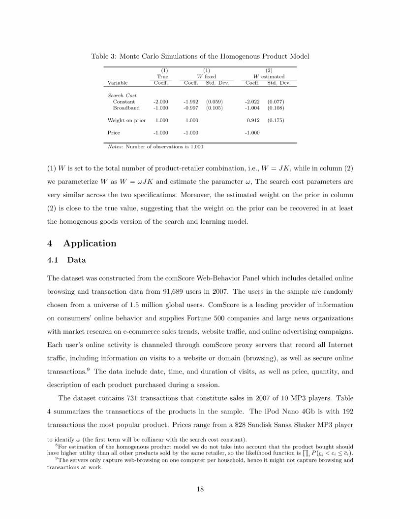
Table 3: Monte Carlo Simulations of the Homogenous Product Model
(1) (1) (2)True W fixed W estimated
Variable Coeff. Coeff. Std. Dev. Coeff. Std. Dev.
Search CostConstant -2.000 -1.992 (0.059) -2.022 (0.077)Broadband -1.000 -0.997 (0.105) -1.004 (0.108)
Weight on prior 1.000 1.000 0.912 (0.175)
Price -1.000 -1.000 -1.000
Notes: Number of observations is 1,000.
(1) W is set to the total number of product-retailer combination, i.e., W = JK, while in column (2)
we parameterize W as W = ωJK and estimate the parameter ω, The search cost parameters are
very similar across the two specifications. Moreover, the estimated weight on the prior in column
(2) is close to the true value, suggesting that the weight on the prior can be recovered in at least
the homogenous goods version of the search and learning model.
4 Application
4.1 Data
The dataset was constructed from the comScore Web-Behavior Panel which includes detailed online
browsing and transaction data from 91,689 users in 2007. The users in the sample are randomly
chosen from a universe of 1.5 million global users. ComScore is a leading provider of information
on consumers’ online behavior and supplies Fortune 500 companies and large news organizations
with market research on e-commerce sales trends, website traffic, and online advertising campaigns.
Each user’s online activity is channeled through comScore proxy servers that record all Internet
traffic, including information on visits to a website or domain (browsing), as well as secure online
transactions.9 The data include date, time, and duration of visits, as well as price, quantity, and
description of each product purchased during a session.
The dataset contains 731 transactions that constitute sales in 2007 of 10 MP3 players. Table
4 summarizes the transactions of the products in the sample. The iPod Nano 4Gb is with 192
transactions the most popular product. Prices range from a $28 Sandisk Sansa Shaker MP3 player
to identify ω (the first term will be collinear with the search cost constant).8For estimation of the homogenous product model we do not take into account that the product bought should
have higher utility than all other products sold by the same retailer, so the likelihood function is∏
i P(ci < ci ≤ ci
).
9The servers only capture web-browsing on one computer per household, hence it might not capture browsing andtransactions at work.
18
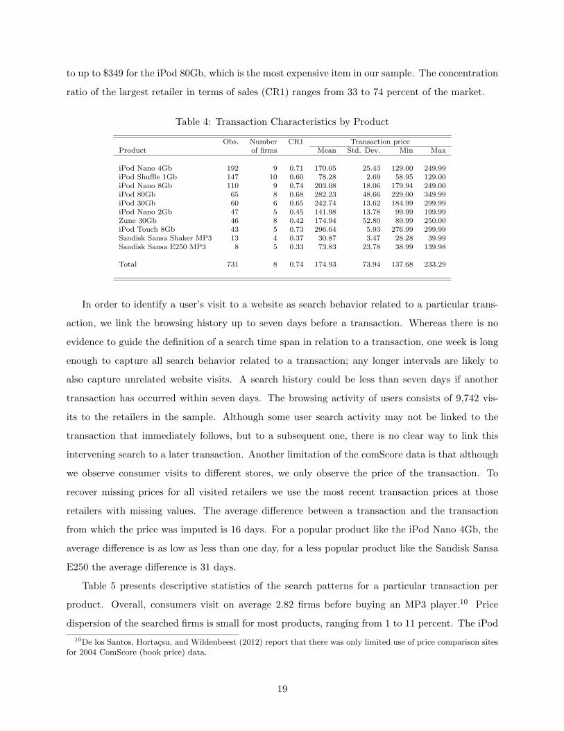
to up to $349 for the iPod 80Gb, which is the most expensive item in our sample. The concentration
ratio of the largest retailer in terms of sales (CR1) ranges from 33 to 74 percent of the market.
Table 4: Transaction Characteristics by Product
Obs. Number CR1 Transaction priceProduct of firms Mean Std. Dev. Min Max
iPod Nano 4Gb 192 9 0.71 170.05 25.43 129.00 249.99iPod Shuffle 1Gb 147 10 0.60 78.28 2.69 58.95 129.00iPod Nano 8Gb 110 9 0.74 203.08 18.06 179.94 249.00iPod 80Gb 65 8 0.68 282.23 48.66 229.00 349.99iPod 30Gb 60 6 0.65 242.74 13.62 184.99 299.99iPod Nano 2Gb 47 5 0.45 141.98 13.78 99.99 199.99Zune 30Gb 46 8 0.42 174.94 52.80 89.99 250.00iPod Touch 8Gb 43 5 0.73 296.64 5.93 276.99 299.99Sandisk Sansa Shaker MP3 13 4 0.37 30.87 3.47 28.28 39.99Sandisk Sansa E250 MP3 8 5 0.33 73.83 23.78 38.99 139.98
Total 731 8 0.74 174.93 73.94 137.68 233.29
In order to identify a user’s visit to a website as search behavior related to a particular trans-
action, we link the browsing history up to seven days before a transaction. Whereas there is no
evidence to guide the definition of a search time span in relation to a transaction, one week is long
enough to capture all search behavior related to a transaction; any longer intervals are likely to
also capture unrelated website visits. A search history could be less than seven days if another
transaction has occurred within seven days. The browsing activity of users consists of 9,742 vis-
its to the retailers in the sample. Although some user search activity may not be linked to the
transaction that immediately follows, but to a subsequent one, there is no clear way to link this
intervening search to a later transaction. Another limitation of the comScore data is that although
we observe consumer visits to different stores, we only observe the price of the transaction. To
recover missing prices for all visited retailers we use the most recent transaction prices at those
retailers with missing values. The average difference between a transaction and the transaction
from which the price was imputed is 16 days. For a popular product like the iPod Nano 4Gb, the
average difference is as low as less than one day, for a less popular product like the Sandisk Sansa
E250 the average difference is 31 days.
Table 5 presents descriptive statistics of the search patterns for a particular transaction per
product. Overall, consumers visit on average 2.82 firms before buying an MP3 player.10 Price
dispersion of the searched firms is small for most products, ranging from 1 to 11 percent. The iPod
10De los Santos, Hortacsu, and Wildenbeest (2012) report that there was only limited use of price comparison sitesfor 2004 ComScore (book price) data.
19
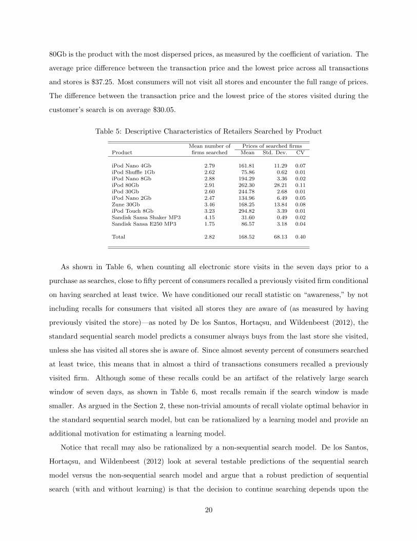
80Gb is the product with the most dispersed prices, as measured by the coefficient of variation. The
average price difference between the transaction price and the lowest price across all transactions
and stores is $37.25. Most consumers will not visit all stores and encounter the full range of prices.
The difference between the transaction price and the lowest price of the stores visited during the
customer’s search is on average $30.05.
Table 5: Descriptive Characteristics of Retailers Searched by Product
Mean number of Prices of searched firmsProduct firms searched Mean Std. Dev. CV
iPod Nano 4Gb 2.79 161.81 11.29 0.07iPod Shuffle 1Gb 2.62 75.86 0.62 0.01iPod Nano 8Gb 2.88 194.29 3.36 0.02iPod 80Gb 2.91 262.30 28.21 0.11iPod 30Gb 2.60 244.78 2.68 0.01iPod Nano 2Gb 2.47 134.96 6.49 0.05Zune 30Gb 3.46 168.25 13.84 0.08iPod Touch 8Gb 3.23 294.82 3.39 0.01Sandisk Sansa Shaker MP3 4.15 31.60 0.49 0.02Sandisk Sansa E250 MP3 1.75 86.57 3.18 0.04
Total 2.82 168.52 68.13 0.40
As shown in Table 6, when counting all electronic store visits in the seven days prior to a
purchase as searches, close to fifty percent of consumers recalled a previously visited firm conditional
on having searched at least twice. We have conditioned our recall statistic on “awareness,” by not
including recalls for consumers that visited all stores they are aware of (as measured by having
previously visited the store)—as noted by De los Santos, Hortacsu, and Wildenbeest (2012), the
standard sequential search model predicts a consumer always buys from the last store she visited,
unless she has visited all stores she is aware of. Since almost seventy percent of consumers searched
at least twice, this means that in almost a third of transactions consumers recalled a previously
visited firm. Although some of these recalls could be an artifact of the relatively large search
window of seven days, as shown in Table 6, most recalls remain if the search window is made
smaller. As argued in the Section 2, these non-trivial amounts of recall violate optimal behavior in
the standard sequential search model, but can be rationalized by a learning model and provide an
additional motivation for estimating a learning model.
Notice that recall may also be rationalized by a non-sequential search model. De los Santos,
Hortacsu, and Wildenbeest (2012) look at several testable predictions of the sequential search
model versus the non-sequential search model and argue that a robust prediction of sequential
search (with and without learning) is that the decision to continue searching depends upon the
20
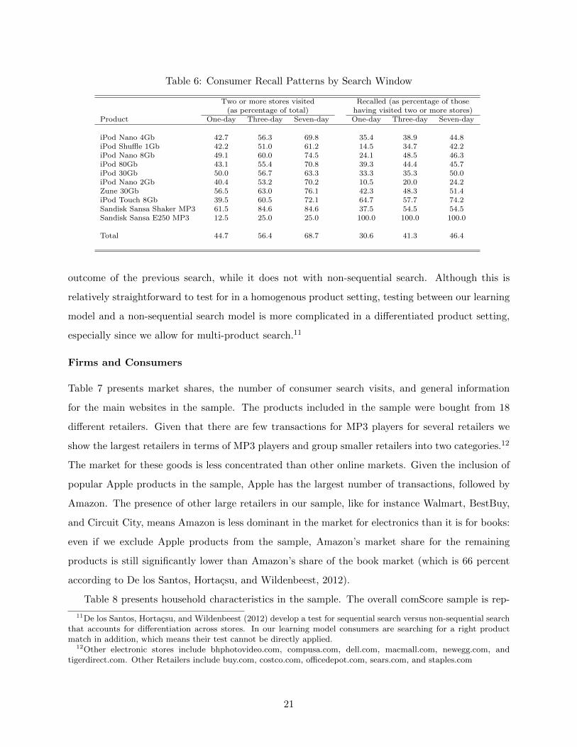
Table 6: Consumer Recall Patterns by Search Window
Two or more stores visited Recalled (as percentage of those(as percentage of total) having visited two or more stores)
Product One-day Three-day Seven-day One-day Three-day Seven-day
iPod Nano 4Gb 42.7 56.3 69.8 35.4 38.9 44.8iPod Shuffle 1Gb 42.2 51.0 61.2 14.5 34.7 42.2iPod Nano 8Gb 49.1 60.0 74.5 24.1 48.5 46.3iPod 80Gb 43.1 55.4 70.8 39.3 44.4 45.7iPod 30Gb 50.0 56.7 63.3 33.3 35.3 50.0iPod Nano 2Gb 40.4 53.2 70.2 10.5 20.0 24.2Zune 30Gb 56.5 63.0 76.1 42.3 48.3 51.4iPod Touch 8Gb 39.5 60.5 72.1 64.7 57.7 74.2Sandisk Sansa Shaker MP3 61.5 84.6 84.6 37.5 54.5 54.5Sandisk Sansa E250 MP3 12.5 25.0 25.0 100.0 100.0 100.0
Total 44.7 56.4 68.7 30.6 41.3 46.4
outcome of the previous search, while it does not with non-sequential search. Although this is
relatively straightforward to test for in a homogenous product setting, testing between our learning
model and a non-sequential search model is more complicated in a differentiated product setting,
especially since we allow for multi-product search.11
Firms and Consumers
Table 7 presents market shares, the number of consumer search visits, and general information
for the main websites in the sample. The products included in the sample were bought from 18
different retailers. Given that there are few transactions for MP3 players for several retailers we
show the largest retailers in terms of MP3 players and group smaller retailers into two categories.12
The market for these goods is less concentrated than other online markets. Given the inclusion of
popular Apple products in the sample, Apple has the largest number of transactions, followed by
Amazon. The presence of other large retailers in our sample, like for instance Walmart, BestBuy,
and Circuit City, means Amazon is less dominant in the market for electronics than it is for books:
even if we exclude Apple products from the sample, Amazon’s market share for the remaining
products is still significantly lower than Amazon’s share of the book market (which is 66 percent
according to De los Santos, Hortacsu, and Wildenbeest, 2012).
Table 8 presents household characteristics in the sample. The overall comScore sample is rep-
11De los Santos, Hortacsu, and Wildenbeest (2012) develop a test for sequential search versus non-sequential searchthat accounts for differentiation across stores. In our learning model consumers are searching for a right productmatch in addition, which means their test cannot be directly applied.
12Other electronic stores include bhphotovideo.com, compusa.com, dell.com, macmall.com, newegg.com, andtigerdirect.com. Other Retailers include buy.com, costco.com, officedepot.com, sears.com, and staples.com
21
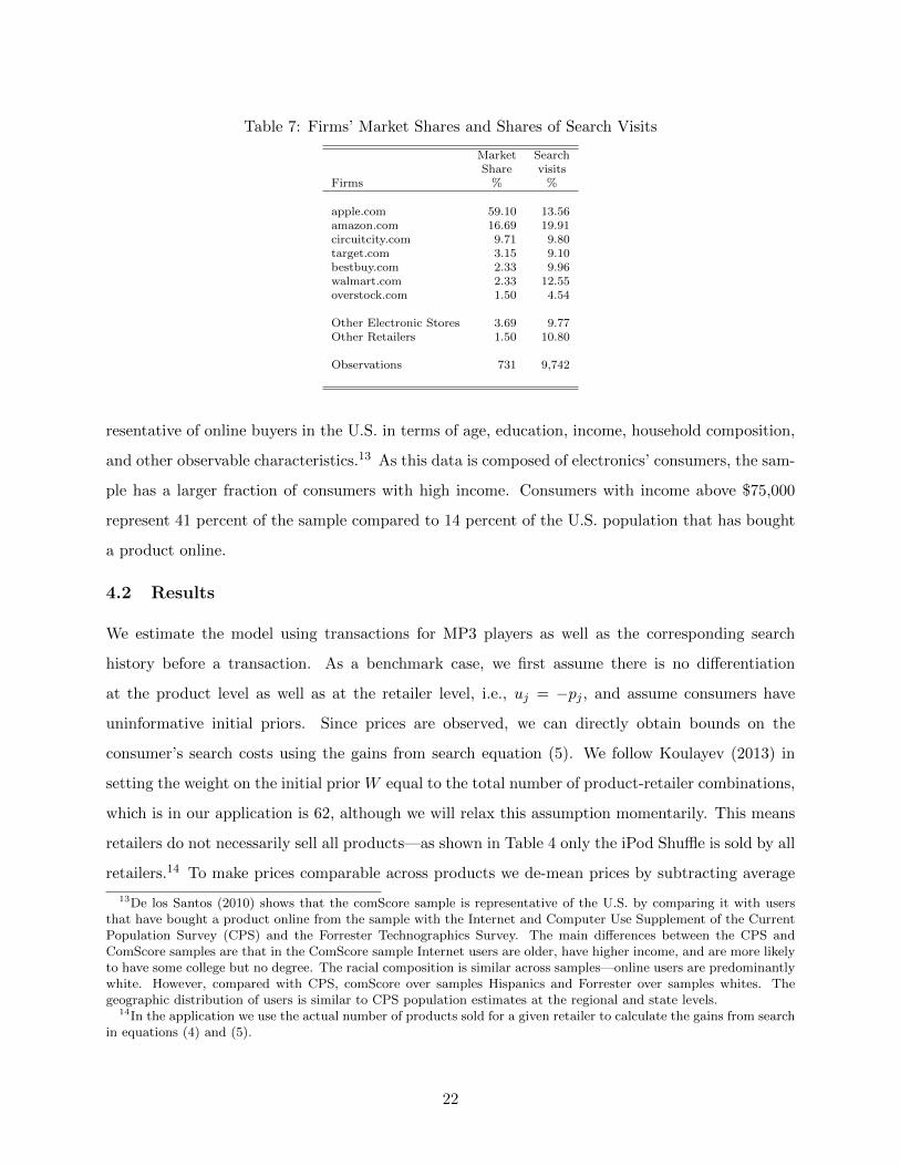
Table 7: Firms’ Market Shares and Shares of Search Visits
Market SearchShare visits
Firms % %
apple.com 59.10 13.56amazon.com 16.69 19.91circuitcity.com 9.71 9.80target.com 3.15 9.10bestbuy.com 2.33 9.96walmart.com 2.33 12.55overstock.com 1.50 4.54
Other Electronic Stores 3.69 9.77Other Retailers 1.50 10.80
Observations 731 9,742
resentative of online buyers in the U.S. in terms of age, education, income, household composition,
and other observable characteristics.13 As this data is composed of electronics’ consumers, the sam-
ple has a larger fraction of consumers with high income. Consumers with income above $75,000
represent 41 percent of the sample compared to 14 percent of the U.S. population that has bought
a product online.
4.2 Results
We estimate the model using transactions for MP3 players as well as the corresponding search
history before a transaction. As a benchmark case, we first assume there is no differentiation
at the product level as well as at the retailer level, i.e., uj = −pj , and assume consumers have
uninformative initial priors. Since prices are observed, we can directly obtain bounds on the
consumer’s search costs using the gains from search equation (5). We follow Koulayev (2013) in
setting the weight on the initial prior W equal to the total number of product-retailer combinations,
which is in our application is 62, although we will relax this assumption momentarily. This means
retailers do not necessarily sell all products—as shown in Table 4 only the iPod Shuffle is sold by all
retailers.14 To make prices comparable across products we de-mean prices by subtracting average
13De los Santos (2010) shows that the comScore sample is representative of the U.S. by comparing it with usersthat have bought a product online from the sample with the Internet and Computer Use Supplement of the CurrentPopulation Survey (CPS) and the Forrester Technographics Survey. The main differences between the CPS andComScore samples are that in the ComScore sample Internet users are older, have higher income, and are more likelyto have some college but no degree. The racial composition is similar across samples—online users are predominantlywhite. However, compared with CPS, comScore over samples Hispanics and Forrester over samples whites. Thegeographic distribution of users is similar to CPS population estimates at the regional and state levels.
14In the application we use the actual number of products sold for a given retailer to calculate the gains from searchin equations (4) and (5).
22

Table 8: Descriptive Statistics of Consumer Characteristics
Mean Std. Dev.
Broadband connection 0.95 0.21Household size 3.31 1.35Children present 0.75 0.43Age
18-20 0.00 0.0621-24 0.02 0.1525-29 0.04 0.2030-34 0.09 0.2935-39 0.13 0.3440-44 0.18 0.3945-49 0.18 0.3950-54 0.14 0.3555-59 0.07 0.2560-64 0.06 0.2365 and over 0.08 0.28
Household incomeLess than $15,000 0.09 0.29$15,000 - $25,000 0.05 0.22$25,000 - $35,000 0.08 0.28$35,000 - $50,000 0.13 0.33$50,000 - $75,000 0.23 0.42$75,000 - $100,000 0.16 0.37More than $100,000 0.25 0.44
RaceWhite 0.94 0.24Black 0.05 0.21Hispanic 0.01 0.10Other 0.00 0.04
Notes: Number of consumers is 637.
product prices.
The search cost bounds give us an idea about the range of search costs for the individuals in our
sample. The dashed curves in Figure 5(a) represent the empirical CDF of our estimate of the search
cost lower bound ci and the upper bound ci.15 The solid line is the empirical CDF of ten (uniform)
draws from the search cost range for each observation and can be interpreted as an average search
cost CDF. The median of this distribution is $3.86, whereas the medians of the lower and upper
bound are $0.75 and $5.56, respectively.
Next, we estimate how search costs relate to household demographics using the maximum like-
lihood procedure described above. The parameters of the search cost specification in equation (8)
are chosen in such a way that the probability that a consumer’s search cost is within correspond-
ing search cost bounds is maximized.16 Figure 5(b) gives the estimated search cost CDF for a
15Since we can only calculate an upper bound if the consumer searches more than once, we set the upper bound ofthose searching once to the maximum upper bound of consumers searching at least twice ($90.74).
16Here we use the same likelihood function as in the Monte Carlo experiments for the homogenous good case, i.e.,we do not factor in the probability that the product bought has the highest utility among all products sold by thesame retailer. See also Footnote 8.
23

10 20 30 40 50c Hin $L
0.2
0.4
0.6
0.8
1.0
CDF
(a) Empirical CDF Lower and Upper Bound
0 10 20 30 40 50c Hin $L0.0
0.2
0.4
0.6
0.8
1.0CDF
(b) Estimed Search Costs
Figure 5: Search Costs Homogeneous Model
specification that lets search cost be a function of a constant, household size, and indicators for 60
years and older, a household income of at least $75,000, and a broadband connection.17 We also
let the weight on the initial prior be a function of the number of product-retailer combinations,
i.e., W = ωJK, where JK = 62 and ω is a parameter to be estimated. The estimated parameter
for weight on the initial prior is 0.071 (standard error 0.017), which means W is estimated to be
slightly over 4. Median search costs are $6.11.
The homogenous product model assumes price is the only factor that is important when buying
an MP3 player. Although this may be true for some buyers, this is unlikely to be the case in
general. In fact, the average difference between the transaction price and the lowest price among
the retailers visited is slightly over $30, which is difficult to explain in the homogenous product
model. This also suggests other attributes than price affect consumer choices, such as product
attributes and retailer characteristics (ease of payment, reliability, speed of shipment, etc.). The
product differentiation model discussed in Section 2.2 can accommodate most of these factors, and
we will focus on this model for the remainder of this section.
Table 9 presents the results for various specifications of the product differentiation model.
Due to the concerns about identification we discussed in the Monte Carlo section, we set the
weight on the initial prior equal to the total number of product-retailer combinations, which means
W = 62. Unobserved product and retailer characteristics may be correlated with prices, which,
if not corrected for, may lead to biased estimates. We deal with this in two ways; firstly, all
17The estimated search cost parameters (standard errors within parenthesis) are:
ln ci = −3.091(0.288)
+ 0.045(0.130)
· Age 60+ − 0.034(0.094)
· Income > 75k + 0.415(0.210)
· Broadband − 0.027(0.034)
· Household Size + ηi.
24
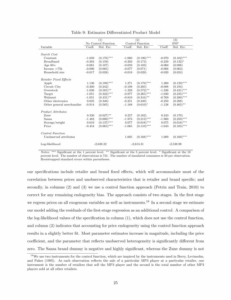
Table 9: Estimates Differentiated Product Model
(1) (2) (3)No Control Function Control Function SNP
Variable Coeff. Std. Err. Coeff. Std. Err. Coeff. Std. Err.
Search CostConstant -1.039 (0.176)∗∗∗ -1.060 (0.196)∗∗∗ -0.970 (0.162)∗∗∗
Broadband -0.204 (0.159) -0.202 (0.174) -0.229 (0.132)∗
Age 60+ -0.061 (0.107) -0.059 (0.103) -0.060 (0.098)Income >75k -0.096 (0.065) -0.077 (0.071) -0.066 (0.063)Household size -0.017 (0.028) -0.018 (0.029) -0.020 (0.024)
Retailer Fixed EffectsApple 1.136 (0.199)∗∗∗ 1.271 (0.179)∗∗∗ 1.260 (0.129)∗∗∗
Circuit City -0.200 (0.242) -0.109 (0.205) -0.088 (0.194)Overstock -1.036 (0.585)∗∗ -1.328 (0.572)∗∗ -1.326 (0.431)∗∗∗
Target -1.051 (0.322)∗∗∗ -0.977 (0.265)∗∗∗ -1.030 (0.235)∗∗∗
Walmart -1.051 (0.431)∗∗ -0.810 (0.344)∗∗ -0.769 (0.280)∗∗∗
Other electronics 0.035 (0.346) -0.251 (0.349) -0.250 (0.298)Other general merchandise -0.914 (0.565) -1.168 (0.610)∗ -1.128 (0.465)∗∗
Product AttributesZune 0.336 (0.027)∗∗ 0.257 (0.162) 0.243 (0.170)Sansa -1.482 (0.000)∗∗∗ -1.973 (0.213)∗∗∗ -1.960 (0.250)∗∗∗
Storage/weight 0.019 (0.137)∗∗∗ 0.077 (0.018)∗∗∗ 0.075 (0.018)∗∗∗
Price -0.454 (0.065)∗∗∗ -1.065 (0.110)∗∗∗ -1.043 (0.105)∗∗∗
Control FunctionUnobserved attributes 1.005 (0.168)∗∗∗ 1.009 (0.160)∗∗∗
Log-likelihood -2,638.22 -2,613.31 -2,538.98
Notes: ∗∗∗ Significant at the 1 percent level. ∗∗ Significant at the 5 percent level. ∗ Significant at the 10percent level. The number of observations is 731. The number of simulated consumers is 50 per observation.Bootstrapped standard errors within parentheses.
our specifications include retailer and brand fixed effects, which will accommodate most of the
correlation between prices and unobserved characteristics that is retailer and brand specific; and
secondly, in columns (2) and (3) we use a control function approach (Petrin and Train, 2010) to
correct for any remaining endogeneity bias. The approach consists of two stages. In the first stage
we regress prices on all exogenous variables as well as instruments.18 In a second stage we estimate
our model adding the residuals of the first-stage regression as an additional control. A comparison of
the log-likelihood values of the specification in column (1), which does not use the control function,
and column (2) indicates that accounting for price endogeneity using the control function approach
results in a slightly better fit. Most parameter estimates increase in magnitude, including the price
coefficient, and the parameter that reflects unobserved heterogeneity is significantly different from
zero. The Sansa brand dummy is negative and highly significant, whereas the Zune dummy is not
18We use two instruments for the control function, which are inspired by the instruments used in Berry, Levinsohn,and Pakes (1995). As each observation reflects the sale of a particular MP3 player at a particular retailer, oneinstrument is the number of retailers that sell the MP3 player and the second is the total number of other MP3players sold at all other retailers.
25

significantly different from zero. Storage per weight has a positive marginal utility. All estimated
search cost parameters have a negative sign, although only the constant is significantly different
from zero at the 1 percent level. Figure 6 plots the estimated search cost CDF using the estimates
in column (2) of Table 9. Search costs are sizable: median search costs are $24.36 and 25 percent
of households have search costs that exceed $48. Although these figures seem relatively large, by
assumption consumers sample all MP3 players sold by a retailer (on average 7 different products)
during one search, which means that search costs per sampled product are substantially lower.
20 40 60 80 100c Hin $L
0.2
0.4
0.6
0.8
1.0
CDF
Figure 6: Estimated Search Cost Distribution
We use a log-normal distribution as the parametric form of the search cost distribution. To
see how sensitive our estimates are to this assumption, we have also estimated the model using
a semi-nonparametric (SNP) approach. In this approach the density is based on flexible Hermite
polynomial functions that approximate arbitrarily closely a large class of sufficiently smooth density
functions (Gallant and Nyckha, 1987). In most applications a normal density is used as a base
function. In our context, where search costs are positive, a log-normal density is a more natural
application. We use the following parametric form for the search cost density:
g(ci;βXi, θ) =
[N∑n=0
θnwn(ci)
]2
N∑n=0
θ2n
, θ ∈ ΘN (12)
26

where ΘN = {θ : θ = (θ0, θ1, . . . , θN ), θ0 = 1}, N is the number of polynomial terms and
w0(ci) = (cσ√
2π)−1/2 exp[−(log ci − βXi)2/4],
w1(ci) = (cσ√
2π)−1/2(log ci − βXi) exp[−(log ci − βXi)2/4],
wn(ci) =[(log ci − βXi)wn−1(ci)−
√n− 1wn−2(ci)
]/√n, for n ≥ 2.
This univariate SNP estimator is equivalent to that in Moraga-Gonzalez, Sandor, and Wilden-
beest (2013), except that we constrain the standard deviation parameter of the associated normal
distribution to be 1. The SNP approach increases the vector of search cost parameters to be esti-
mated by maximum likelihood to {β, θ1, . . . , θN}. The number of SNP parameters N can be made
arbitrarily large as the number of observations increases to infinity; in our application we follow
recommendations by Fenton and Gallant (1996) and set N = 4, which equals the closest integer to
the fifth root of the total number of observations. A comparison of log-likelihood values between
columns (2) and (3) suggests the fit has improved substantially by allowing for the more flexible
SNP estimator, although most parameter estimates appear unaffected. However, the estimated
search cost distribution may still be different since it now also depends on the additional SNP pa-
rameters we have estimated.19 Indeed, a comparison of the two estimated search cost distributions
in Figure 7(a) shows that search costs are higher at especially the lower end of the distribution for
the SNP specification.
log-normal
SNP
20 40 60 80 100c Hin $L
0.2
0.4
0.6
0.8
1.0
CDF
(a) SNP
learning
no learning
20 40 60 80 100c Hin $L
0.2
0.4
0.6
0.8
1.0
CDF
(b) No learning
Figure 7: Estimated Search Costs SNP and No-Learning Model
19The parameter estimates are (bootstrapped standard errors within parentheses) θ1 = −0.117 (0.018), θ2 =−0.507 (0.005), θ3 = 0.090 (0.013), θ4 = 0.302 (0.008).
27

Alternative Specifications
Table 10 gives parameter estimates for various alternative specifications. Our data only allows to
observe visits to retailers at the domain level—for all estimates so far we have linked visits to a
retailer for up to seven days prior to a MP3-player transaction as being related to the purchase of
the MP3-player. To see how sensitive our estimates are to assumptions about the length of this
window, we have also estimated the model assuming only visits to a retailer in the three days prior
to a purchase are related. The results assuming this different window are shown in column (1)
of Table 10. Except for the search cost constant, which is higher for the three-day window, all
parameter estimates are very similar to the results when assuming a seven-day window, as reported
in column (2) of Table 9. The difference in search cost estimates is intuitive: a lower number
of retailers is visited when assuming a smaller window, which can only be rationalized by having
higher search cost estimates.
Table 10: Alternative Specifications
(1) (2) (3) (4)Three-Day Window Uninformative Prior W = 31 No Learning
Variable Coeff. Std. Err. Coeff. Std. Err. Coeff. Std. Err. Coeff. Std. Err.
Search CostConstant -0.701 (0.202)∗∗∗ -0.796 (0.345)∗∗ -1.266 (0.185)∗∗∗ -0.742 (0.133)∗∗∗
Broadband -0.221 (0.173) -0.338 (0.303) -0.217 (0.177) -0.210 (0.115)∗
Age 60+ -0.194 (0.122) -0.126 (0.256) -0.062 (0.118) -0.031 (0.103)Income >75k -0.083 (0.094) -0.178 (0.188) -0.095 (0.078) -0.049 (0.068)Household size -0.027 (0.032) -0.008 (0.074) -0.017 (0.032) -0.019 (0.025)
Retailer Fixed EffectsApple 1.478 (0.170)∗∗∗ 1.148 (0.120)∗∗∗ 1.454 (0.177)∗∗∗ 0.875 (0.127)∗∗∗
Circuit City -0.056 (0.214) -0.404 (0.182)∗∗ -0.105 (0.248) -0.219 (0.151)Overstock -1.133 (0.521)∗∗ -1.580 (0.259)∗∗∗ -1.419 (0.428)∗∗∗ -1.055 (0.261)∗∗∗
Target -0.870 (0.301)∗∗∗ -0.950 (0.201)∗∗∗ -1.251 (0.369)∗∗∗ -0.788 (0.170)∗∗∗
Walmart -1.745 (0.557)∗∗∗ -0.638 (0.232)∗∗∗ -1.160 (0.417)∗∗∗ -0.499 (0.186)∗∗∗
Other electronics -0.059 (0.388) -0.556 (0.220)∗∗ -0.282 (0.441) -0.196 (0.256)Other general merchandise -1.439 (5.211) -1.323 (0.331)∗∗∗ -1.441 (0.862)∗ -0.626 (0.201)∗∗∗
Product AttributesZune 0.252 (0.176) 0.330 (0.134)∗∗ 0.266 (0.163) 0.252 (0.166)Sansa -1.948 (0.246)∗∗∗ -1.805 (0.241)∗∗∗ -1.967 (0.261)∗∗∗ -1.710 (0.255)∗∗∗
Storage/weight 0.079 (0.018)∗∗∗ 0.086 (0.019)∗∗∗ 0.079 (0.015)∗∗∗ 0.085 (0.019)∗∗∗
Price -1.063 (0.118)∗∗∗ -1.109 (0.135)∗∗∗ -1.055 (0.117)∗∗∗ -1.130 (0.140)∗∗∗
Control FunctionUnobserved attributes 1.023 (0.165)∗∗∗ 1.091 (0.203)∗∗∗ 1.035 (0.173)∗∗∗ 1.054 (0.212)∗∗∗
Log-likelihood -2,392.52 -2,565.68 -2,566.44 -2,736.33
Notes: ∗∗∗ Significant at the 1 percent level. ∗∗ Significant at the 5 percent level. ∗ Significant at the 10 percent level. Thenumber of observations is 731. The number of simulated consumers is 50 per observation. Bootstrapped standard errors withinparentheses. All specifications have retailer specific dummies.
The second specification in Table 10 we use a uniform distribution instead of type I extreme
28

value distribution as the initial prior. Here we assume the lower and upper bound of the uniform are
known to the consumer and correspond to the lowest and highest utility in the market. Estimated
search costs are higher than when assuming consumers have rational initial priors. Since a uniform
distribution puts equal weight to all utility values in excess of the highest utility observed so far,
the gains from search are uniformly higher, which means search costs need to be higher in order to
rationalize observed search patterns.
In the third specification in Table 10 we set W = 31, which means the weight on the initial
prior is half of what we assume in our main specification. The estimated search cost constant is
slightly lower; the rest of the estimated parameters do not change much in comparison to those
reported in column (2) of Table 9. Although not reported, estimates assuming W = 93 are very
similar to the main specification as well.
In our final specification in Table 10, we fit a standard sequential search model to the data
by assuming there is no Bayesian updating. This is equivalent to setting t = 0 in equation (2)
and means consumers know the utility distribution with certainty. As shown in the last column of
Table 10 the model does worse in terms of fitting the data. Part of this is explained by the model
being unable to account for recall patterns. The estimates are also quite different: according to
the learning model median search costs are $24.36, while in the model with no updating median
search costs are with $31.73 more than 30 percent higher. The difference in search cost estimates
can also be seen in Figure 7(b), which plots the search cost CDFs for both specifications.
29

5 Conclusions
In this paper we have presented a methodology to estimate a consumer search model with learning.
The distribution of utilities is assumed to be unknown to consumers and is learned in the search
process by Bayesian updating Dirichlet process priors. We have shown how to use information on
the sequence of searches as well as prices to derive expressions for the bounds on a consumer’s
search costs. We relate search costs to the characteristics of households in our sample and find
search costs to be sizable: our estimates indicate that search costs are on average slightly over
$24. Estimated search costs are uniformly lower than in a sequential search model with a known
distribution of utilities. Moreover, the learning model gives a better fit to the data than the model
in which there is no updating.
The Monte Carlo experiments have shown that in the case of homogenous products, our es-
timation method allows us to recover how much weight consumers put on their initial priors.
Nevertheless, it is difficult to say anything definitive on the identification of the prior in the more
realistic product differentiation model. We have shown that to estimate our model, the number
of searches as well as information from the last search is needed: the search cost bounds in our
model are derived from the gains from search when actually purchasing the product and the period
before that. We are hopeful that using the entire sequence of searches will help in identifying the
importance of learning in a product differentiation setting, and leave this for future research.
30

References
Ackerberg, Daniel A.: “Advertising, Learning, and Consumer Choice in Experience Good Markets:
An Empirical Examination,” International Economic Review 44, pp. 1007–1040, 2003.
Berry, Steven, James Levinsohn, and Ariel Pakes: “Automobile Prices in Market Equilibrium,”
Econometrica 63, pp. 841–890, 1995.
Bikhchandani, Sushil and Sunil Sharma: “Optimal Search with Learning,” Journal of Economic
Dynamics and Control 20, pp. 333–359, 1996.
Chernew, Michael, Gautam Gowrisankaran, and Dennis P. Scanlon: “Learning and the Value of
Information: Evidence from Health Plan Report Cards,” Journal of Econometrics 144, pp.
156–174, 2008.
Chou, Chien-fu and Gabriel Talmain: “Nonparametric Search,” Journal of Economic Dynamics
and Control 17, pp. 771–784, 1993.
Crawford, Gregory S. and Matthew Shum: “Uncertainty and Learning in Pharmaceutical Demand,”
Econometrica 73, pp. 1137–1173, 2005.
Dana, James D.: “Learning in an Equilibrium Search Model,” International Economic Review 35,
pp. 745–771, 1994.
De los Santos, Babur: “Consumer Search on the Internet,” mimeo, 2010.
De los Santos, Babur, Ali Hortacsu, and Matthijs Wildenbeest: “Testing Models of Consumer
Search Using Data on Web Browsing and Purchasing Behavior,” American Economic Review
102, pp. 2955–2980, 2012.
Erdem, Tulin and Michael P. Keane: “Decision-Making Under Uncertainty: Capturing Dynamic
Brand Choice Processes in Turbulent Consumer Goods Markets,” Marketing Science 15, pp.
1–20, 1996.
Fenton, Victor M. and A. Roland Gallant: “Qualitative and Asymptotic Performance of SNP
Density Estimators,” Journal of Econometrics 74, pp. 77–118, 1996.
Ferguson, Thomas S.: “A Bayesian Analysis of Some Nonparametric Problems,” The Annals of
Statistics 1, pp. 209–230, 1973.
31
Gallant, A. Ronald and Douglas W. Nychka: “Semi-Nonparametric Maximum Likelihood Estima-
tion,” Econometrica 55, pp. 363–390, 1987.
Gastwirth, Joseph L. : “On Probabilistic Models of Consumer Search for Information,” Quarterly
Journal of Economics 90, pp. 38–50, 1976.
Haubl, Gerald, Benedict G. C. Dellaert, and Bas Donkers: “Tunnel Vision: Local Behavioral
Influences on Consumer Decisions in Product Search,” Marketing Science 29, pp. 438–455,
2010.
Hong, Han and Matthew Shum: “Using Price Distributions to Estimate Search Costs,” RAND
Journal of Economics 37, pp. 257–275, 2006.
Hortacsu, Ali and Chad Syverson: “Product Differentiation, Search Costs, and Competition in
the Mutual Fund Industry: a Case Study of S&P 500 Index Funds,” Quarterly Journal of
Economics 119, pp. 403–456, 2004.
Koulayev, Sergei: “Search with Dirichlet Priors: Estimation and Implications for Consumer De-
mand,” Journal of Business & Economic Statistics 31, pp. 226–239, 2013.
Koulayev, Sergei: “Estimating Demand in Search Markets: the Case of Online Hotel Bookings,”
forthcoming in RAND Journal of Economics.
McCall, John J.: “Economics of Information and Job Search,” Quarterly Journal of Economics 84,
pp. 113–126, 1970.
Moraga-Gonzalez, Jose Luis and Matthijs R. Wildenbeest: “Maximum Likelihood Estimation of
Search Costs,” European Economic Review 52, pp. 820–848, 2008.
Moraga-Gonzalez, Jose Luis, Zsolt Sandor, and Matthijs R. Wildenbeest: “Semi-Nonparametric
Estimation of Consumer Search Costs,” Journal of Applied Econometrics 28, pp. 1205–1223,
2013.
Mortensen, Dale T.: “Job Search, the Duration of Unemployment and the Phillips Curve,” Amer-
ican Economic Review 60, pp. 847–862, 1970.
Petrin, Amil, and Kenneth Train: “A Control Function Approach to Endogeneity in Consumer
Choice Models,” Journal of Marketing Research 47, pp. 3–13, 2010.
32

Rosenfield, Donald B. and Roy D. Shapiro: “Optimal Adaptive Price Search,” Journal of Economic
Theory 25, pp. 1–20, 1981.
Rothschild, Michael: “Searching for the Lowest Price when the Distribution of Prices is Unknown,”
Journal of Political Economy 82, pp. 689–711, 1974.
Stigler, George: “The Economics of Information,” Journal of Political Economy 69, pp. 213–225,
1961.
Wildenbeest, Matthijs R.: “An Empirical Model of Search with Vertically Differentiated Products,”
RAND Journal of Economics 42, pp. 729–757, 2011.
33

Appendix
Additional Details on the Derivation of Equation (4)
In general, the expected maximum utility out of J draws from distribution H(u) is given by
E
[maxj∈J{uij}
]=
∫ ∞−∞
ud
du
∏j∈J
H(u− δj)
du;
=
∫u∑j∈J
h(u− δj)∏r∈J\j
H(u− δr)
du;
=
∫u∑j∈J
exp[−((u− δj) + exp[−(u− δj)])]∏r∈J\j
exp [− exp [−(u− δr)]]
du;
= γ + log
∑j∈J
exp[δj ]
.
Note that E [maxj∈J {uij}] is relevant when searching non-sequentially, for instance when the deci-
sion is whether to search J or J + 1 times. In our setting the decision is whether to sample J firms
given that the utility at hand is uit. Just focusing on this, and ignoring the W/(W + t) term, this
means the gains from search equation is
G(uit) =
∫ ∞uit
(u− uit)d
du
∏j∈J
H(u− δj)
du.
We can rewrite this integral as to sum of three separate integrals:
G(uit) =
∫ ∞−∞
ud
du
∏j∈J
H(u− δj)
du−∫ ∞−∞
uitd
du
∏j∈J
H(u− δj)
du−∫ uit
−∞(u−uit)
d
du
∏j∈J
H(u− δj)
du.
The first integral is the expected maximum utility out of J draws from H(u), which, using the
results from above, has the closed-form solution γ + log(∑
j∈J exp[δj ])
. The second integral is
just the reference utility uit. Finally, the last integral reflects a situation in which the maximum
utility of J draws is less than uit, so the consumer will find it optimal to stick to uit. This, integral
does not have a closed-form solution, but can be described by the exponential integral function
evaluated at a =∑
j∈J exp [δj − uit], i.e., the integral equals −∫∞a e−x/x dx. Therefore, the gains
from search equation simplifies to
G(uit) = γ + log
∑j∈J
exp[δj ]
− (uit − ∫ ∞a
e−x/x dx
). (13)
34
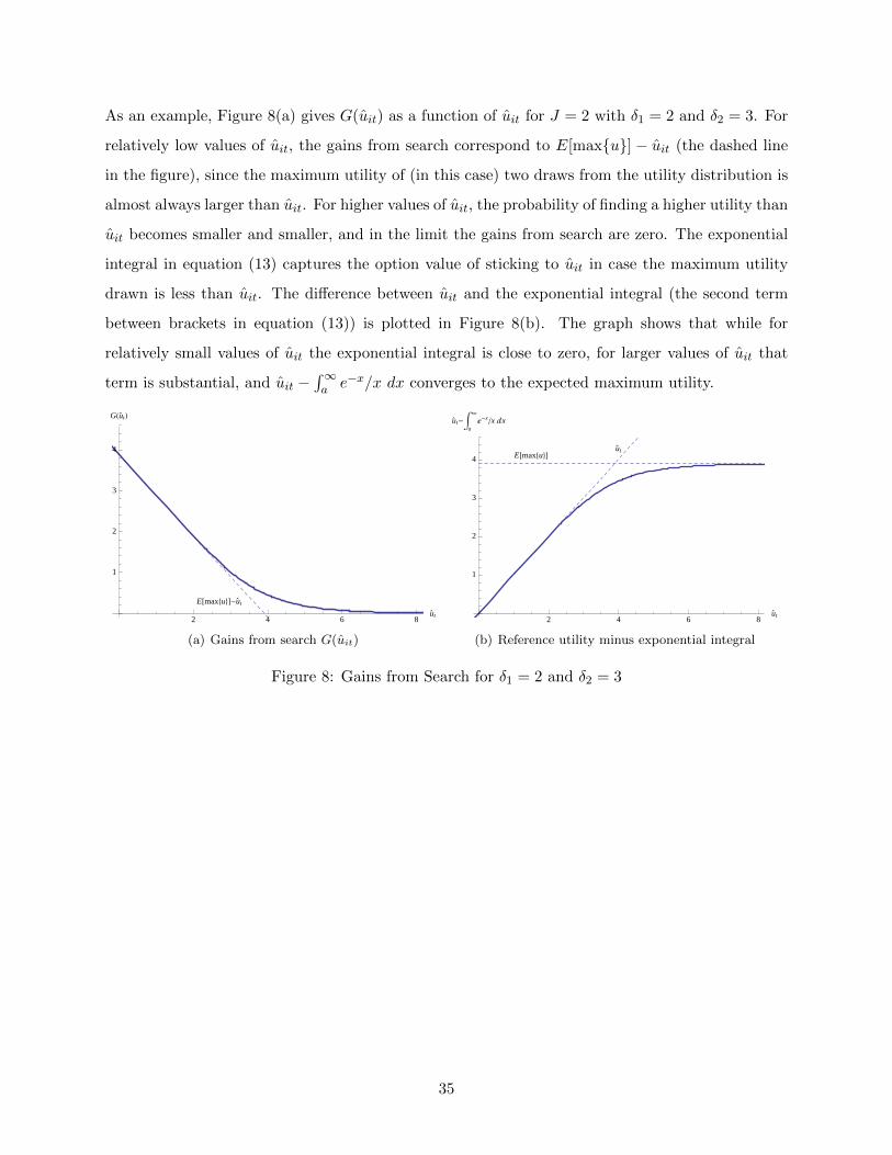
As an example, Figure 8(a) gives G(uit) as a function of uit for J = 2 with δ1 = 2 and δ2 = 3. For
relatively low values of uit, the gains from search correspond to E[max{u}] − uit (the dashed line
in the figure), since the maximum utility of (in this case) two draws from the utility distribution is
almost always larger than uit. For higher values of uit, the probability of finding a higher utility than
uit becomes smaller and smaller, and in the limit the gains from search are zero. The exponential
integral in equation (13) captures the option value of sticking to uit in case the maximum utility
drawn is less than uit. The difference between uit and the exponential integral (the second term
between brackets in equation (13)) is plotted in Figure 8(b). The graph shows that while for
relatively small values of uit the exponential integral is close to zero, for larger values of uit that
term is substantial, and uit −∫∞a e−x/x dx converges to the expected maximum utility.
E@max8u<D-u`
t
2 4 6 8u`
t
1
2
3
4
GHu` tL
(a) Gains from search G(uit)
E@max8u<Dut
2 4 6 8ut
1
2
3
4
ut-àa
¥
ã-x�x âx
(b) Reference utility minus exponential integral
Figure 8: Gains from Search for δ1 = 2 and δ2 = 3
35