Learning to Search:Functional Gradient Techniques

for Imitation Learning

Nathan D. RatliffRobotics Institute

Carnegie Mellon UniversityPittsburgh, PA 15213

ndr@ri.cmu.edu

David SilverRobotics Institute

Carnegie Mellon UniversityPittsburgh, PA 15213dsilver@ri.cmu.edu

J. Andrew BagnellRobotics Institute and Machine Learning

Carnegie Mellon UniversityPittsburgh, PA 15213dbagnell@ri.cmu.edu

Abstract

Programming robot behavior remains a challenging task. While it is often easy to abstractly define oreven demonstrate a desired behavior, designing a controller that embodies the same behavior is difficult,time consuming, and ultimately expensive. The machine learning paradigm offers the promise of enabling“programming by demonstration” for developing high-performance robotic systems. Unfortunately, many“behavioral cloning” (Bain & Sammut, 1995; Pomerleau, 1989; LeCun et al., 2006) approaches that utilizeclassical tools of supervised learning (e.g. decision trees, neural networks, or support vector machines) donot fit the needs of modern robotic systems. These systems are often built atop sophisticated planningalgorithms that efficiently reason far into the future; consequently, ignoring these planning algorithms inlieu of a supervised learning approach often leads to myopic and poor-quality robot performance.

While planning algorithms have shown success in many real-world applications ranging from leggedlocomotion (Chestnutt et al., 2003) to outdoor unstructured navigation (Kelly et al., 2004; Stentz et al.,2007), such algorithms rely on fully specified cost functions that map sensor readings and environmentmodels to quantifiable costs. Such cost functions are usually manually designed and programmed. Re-cently, a set of techniques has been developed that explore learning these functions from expert humandemonstration. These algorithms apply an inverse optimal control approach to find a cost function forwhich planned behavior mimics an expert’s demonstration.

The work we present extends the Maximum Margin Planning (MMP) (Ratliff et al., 2006a) frame-work to admit learning of more powerful, non-linear cost functions. These algorithms, known collectivelyas LEARCH (LEArning to seaRCH ), are simpler to implement than most existing methods, more effi-cient than previous attempts at non-linearization (Ratliff et al., 2006b), more naturally satisfy commonconstraints on the cost function, and better represent our prior beliefs about the function’s form. Wederive and discuss the framework both mathematically and intuitively, and demonstrate practical real-world performance with three applied case-studies including legged locomotion, grasp planning, andautonomous outdoor unstructured navigation. The latter study includes hundreds of kilometers of au-tonomous traversal through complex natural environments. These case-studies address key challengesin applying the algorithm in practical settings that utilize state-of-the-art planners, and which may beconstrained by efficiency requirements and imperfect expert demonstration.

1

Figure 1: Imitation learning applies to a wide variety of robotic platforms. This figure shows a few of the robots

on which the imitation learning algorithms discussed here have been implemented. From left to right, we have (1)

an autonomous ground vehicle build by the National Robotics Engineering Center (NREC) known as Crusher, (2)

Boston Dynamics’s LittleDog quadrupedal robot, and (3) Barrett Technologies’s WAM arm, wrist, and 10-DOF hand.

1 Introduction

Encoding a desired behavior in a robot is a difficult task. Programmers often understand intuitively howthey want a robot to behave in various situations, but uncovering a set of parameters for a modern systemwhich embodies that behavior can be time consuming and expensive. When programming a robot’s behaviorresearchers often adopt an informal process of repeated “guess-and-check”. For a skilled practitioner, thisprocess borders on algorithmic. Imitation learning studies the algorithmic formalization for programmingbehavior by demonstration. Since many robot behaviors are defined in terms of optimization, such as thosedesigned around optimal planners, imitation learning can be modeled as identifying optimization criteriathat make the expert look optimal. This intuition is formalized by the Maximum Margin Planning (MMP)framework (Ratliff et al., 2006a) which defines a convex objective that measures the sub-optimality withrespect to an expert’s demonstrated policy.

MMP arises through a reduction of imitation learning to a form of machine learning called structuredprediction. Structured prediction studies problems in which making multiple predictions simultaneously canimprove accuracy. The term “structure” refers to the relationships among the predictions that make thispossible. For instance, attempting to predict independently whether individual states occur along an optimalpath in a graph has little hope of success without accounting for the connectivity of the graph.

Robotics researchers naturally exploit this connectivity when developing efficient planning algorithms.By reducing imitation learning to a structured prediction problem, we leverage this body of work withinlearning to capture the problem’s structure and improve prediction. Algorithms that solve MMP imitate bylearning to predict the entire sequence of actions that an expert would take toward a goal.

This work presents a unified view of imitation learning in this structured prediction framework by buildingon and extending the techniques of (Ratliff et al., 2006a; Ratliff et al., 2006b). We present a family offunctional gradient techniques for this problem, including a novel exponentiated functional gradient algorithmthat extends the techniques of (Kivinen & Warmuth, 1997) to function spaces in a way analogous to gradientboosting (Mason et al., 1999; Friedman, 1999a). This algorithm was first test empirically in (Ratliff et al.,2007b) and is derived and analyzed in detail here for the first time. The techniques presented in this workprovide more flexibility in learned cost functions than those considered in previous work using a linearcombination of features. Consequently, the approach presented reduces the engineering burden and increasethe applicability of imitation learning– and structured prediction generally– to real-world problems.

The LEARCH family of algorithms has been successfully demonstrated previously on a range of structuredprediction and imitation learning problems including programming by demonstration (Ratliff et al., 2006a;Silver et al., 2008), LADAR classification (Munoz et al., 2008; Ratliff et al., 2007a), sequence prediction(Ratliff et al., 2007a), and heuristic learning (Ratliff et al., 2006b). Figure 1 depicts three robotic platformson which these algorithms have been applied. We summarize here a few imitation learning applications toillustrate our approach and provide a comparison of the between different algorithms in the LEARCH family.

2

1.1 A short history of imitation learning

Before formally defining our imitation learning framework, we review prior work in the field and map out aprogression of algorithms that form the foundation for this work. A full survey of the numerous approachesto imitation learning studied in the literature is beyond the scope of this paper, but we point the interestedreader to (Argall et al., 2009) for a detailed overview. Of note is the work of Schaal and Atkeson (Schaal &Atkeson, 1994; Atkeson et al., 1995) whose algorithms develop control strategies within a given environmentusing trajectory demonstrations. Additionally, (Calinon et al., 2007) and (Hersch et al., 2008) have developedtechniques that allow generalization to alternative goals within a given domain. Our work focuses on thebroader problem of generalizing control between distinct domains; we therefore do not discuss this literaturein detail here.

The first notable examples of imitation learning came in the form of action prediction: predict the bestaction to take now given features of the current state of the environment and robot. Perhaps the best knownsystem built using this paradigm was ALVINN (Pomerleau, 1989). Pomerleau et. al. trained a neuralnetwork to predict the desired steering angle of a vehicle given an image of the road ahead.

Unfortunately, such a system is inherently myopic. This form of imitation learning assumes that allinformation necessary to make a decision at the current state can be easily encoded into a single vector offeatures that enables prediction with a relatively simple, learned function. However, this is often particularlydifficult because the features must encode information regarding the future long-term consequences of takingan action. Under this framework, much of the work that we would like learning to handle is pushed ontothe engineer in the form of feature extraction.

Further, as traditional supervised learning tools do not reason about the structure of making sequentialdecisions, it is often the case that small errors in prediction translate to large errors in performance. Even aclassifier trained to achieve very high accuracy agreement with example decisions is likely to choose a seriesof actions that is not a valid path from a start to a distant goal. Rather than minimizing a short-sightedloss over individual actions a successful algorithm must learn to imitate entire sequences of actions.

Recently, a new approach based on leveraging existing optimal control and planning algorithms has beendeveloped for addressing the imitation learning problem. The concept is to leverage the older notion ofinverse optimal control (Kalman, 1964; Boyd et al., 1994; Anderson & Moore, 1990): imitation learning isachieved by first recovering a cost function by observing an expert perform a task, and then executing newtasks using an optimal controller/planner to minimize that learned cost function. Inverse optimal controlwas first proposed– and solved for linear systems with scalar input– by Kalman (Kalman, 1964) and solutionsof increasing generality were developed over the ensuing years culminating in the work of (Boyd et al., 1994).

Linear systems theory is insufficient to handle the generality of decision making problems considered inrobotics, however. In this work, we consider the encompassing framework of Markov Decision Processes(MDPs). MDPs model the environment as a set of states connected by an action model, which defines theprobability of arriving at any new state s′ given that the agent started in state s and applied action a. Thisprobability is Markovian: that is, it does not depend on previous states visited. Associated with an MDPis a reward (or cost) function, often defined over state-action pairs, which specifies quantitatively how muchreward is received when an agent takes a particular action from a given state.

The first approaches to recovering a cost function for general, discrete MDPs by observing a demonstratedbehavior were suggested in (Ng & Russell, 2000; Abbeel & Ng, 2004). In this formulation, it is assumedthat the agent observed is truly acting in the MDP and the goal is to find a policy that accrues the samelong-term cumulative reward as the demonstrated behavior. Unfortunately, as the authors point out, theproblem is fundamentally ill-posed. We can see one example of this by noting that, given any MDP whosereward function is everywhere zero, all policies accrue the same long-term cumulative reward– namely zero.In (Abbeel & Ng, 2004), however, the authors note that if the reward function is a linear combinationof features, an alternative, more practical, condition known as “feature count matching”, can be posed toavoid this fundamental problem. Consider, for simplicity, the case of deterministic planning. We first definefsa as the feature vector over a state-action pair (s, a), and choose the corresponding reward to be a linearcombination of these features csa = wT fsa. Straightforward calculation shows that if the sum of features (i.e.∑

(s,a)∈ξ fsa) along a path ξ taken by the planner agrees with the same sum taken over the demonstrated

path, by linearity both must achieve the same reward.

3

Unfortunately, while this work has provided an important demonstration that the inverse optimal controlproblem can be efficiently solved, it has a number of significant short-comings. First, the feature matchingrequirement is, in a sense, simultaneously over-constrained and ill-posed. It is over-constrained in the sensethat there is almost never an optimal policy that achieves demonstrated feature counts on real problems–the experts demonstrating the desired behavior are not actually acting in the MDP we use to define ourcontrol problem, and even were they to be, they are rarely optimal. As such, we are left with an ill-posedproblem, for which (Abbeel & Ng, 2004) offers specific algorithmic approaches for finding one of an infinitenumber of randomized policies (in the specific case actually a mixture of policies where we choose randomlywhich controller to execute on the initial step) that achieve the desired feature counts. Such policies candiffer wildly in the behavior they actually manifest. Recently, (Ziebart et al., 2008) resolved these difficultiesin the feature count matching approach by connecting the inverse optimal control problem to probabilisticmodeling and the Maximum Entropy Method (Jaynes, 2003) and provided a unique, optimal, stochasticpolicy.

Further, while defining inverse reinforcement learning as the problem of matching cumulative featurecounts is sensible when the reward function is a linear combination of features, the condition is no longerrelevant for more general nonlinear reward functions. Many of the imitation learning algorithms that wediscuss below are nonlinear and consequently require a fundamentally different problem definition. Wepropose a more general definition of imitation learning by inverse optimal control that attempts to directlymimic behavior according to a loss function measuring deviation from the behavior we desire (and is agnosticas to whether the demonstrating agent is truly trying to minimize a reward function in an MDP), providesapproximation and regret (Ratliff et al., 2007a) guarantees on the resulting solutions, and admits a particularclass of non-linear loss functions. While LEARCH has close connections with the notion of achieving similarfeature counts when we specialize to linear reward functions, it returns only a single, deterministic policyfor solving the problem.

We have applied the general LEARCH framework in settings ranging from quadrupedal locomotion tolong-range outdoor autonomous navigation. These results developed over the preceding three years (Ratliffet al., 2006a; Ratliff et al., 2006b; Ratliff et al., 2007a; Silver et al., 2008) are, to the best of our knowledge,the first practical applications of inverse optimal control algorithms to robotic systems. Sections 5 and 6present some of these case studies; more recently, extensions to hierarchical learning problems for quadrupedallocomotion (Kolter et al., 2008) have additionally supported inverse optimal control’s status as a preferredapproach to imitation learning.

1.2 An operational introduction to LEArning to seaRCH

We begin with an overview of our MMP framework for imitation learning and discuss one algorithm inthe LEARCH family from an intuitive, operational view. These sections are designed to emphasize theconceptual and operational simplicity of LEARCH before presenting more detailed formal derivations. Thebasic approach is sufficiently intuitive that in the next section we describe it first as it might be practicallyimplemented.

Let D = {(Mi, ξi)}Ni=1 denote a set of examples, each consisting of an MDP Mi (excluding a specificreward function) and an example trajectory ξi between start and goal points. Figure 2 visually depicts thetype of training data we consider here for imitation learning problems. Often, we can think of an exampleas a path between a pair of end points. Each MDP is imbued with a feature function that maps each state-action pair (s, a) in the MDP to a feature vector fsai ∈ Rd. This feature vector represents a set of d sensorreadings (or derived quantities) that distinguish one state from the next.

For clarity, we consider here only the deterministic case in which the MDP can be viewed as a directedgraph (states connected by actions). Planning between a pair of points in the graph can be implementedefficiently using combinatorial planning algorithms such as Dijkstra or A*. In this setting, it is common toconsider costs rather than rewards. Intuitively, a cost can be thought of simply as a negative reward; theplanner must minimize the cumulative cost of the plan rather than maximize the cumulative reward. Forthe moment, we ignore positivity constraints on the cost function required by many combinatorial plannerssuch as A*, but we will address these constraints formally later on.

4

Figure 2: This figure demonstrates the flavor of the training data considered here in the context of imitation learning.

In this case, a human expert specified by hand examples of the path (red) that a mobile robot should take between

pairs of end points (green) through overhead satellite images. These example paths demonstrate the form of training

data used for the outdoor navigational planning experiment discussed in section 6.

Intuitively, the maximum margin planning algorithm iteratively refines the cost function c : Rd → R

in order to make the example trajectories optimal. Since there is a feature vector associated with eachstate-action pair, a cost map (i.e. a mapping from state-action pairs to costs) can be generated for eachMi by evaluating the cost function at each state-action feature vector fsai . Given the cost map, any blackbox deterministic planning algorithm can be run to determine the optimal path. Since the example pathξi is a valid path, the minimum cost path returned by the planning algorithm will usually have lower cost.In essence, the goal of the learning algorithm is to find a cost function for which the example path is theminimum cost path. Therefore, we can use the gap between the cost of the example path and the cost ofthe minimum cost path as a measure of sub-optimality.

During each iteration, the maximum margin planning algorithm suggests local corrections to the costfunction to progress toward minimizing the gap. It does this by suggesting that the cost function be increasedin regions of the feature space encountered along the planned path, and decreased in regions of the featurespace encountered along the example path.1

Specifically, for each example i, the algorithm considers two paths: the example path ξi, and the plannedpath ξ∗i = arg minξ∈Ξi

∑(sa)∈ξ c(f

sai ). In order to decrease the difference between the example path’s cost

and the planned path’s cost, the algorithm needs to modify the cost function so that the cost of the plannedpath increases and the cost of the example path decrease. For each path, the path cost is simply a sum ofstate-action costs encountered along the way, which are each generated by evaluating the cost function atthe feature vector fsai associated with that state-action pair. The algorithm can, therefore, raise or lowerthe cost of this path incrementally simply by increasing or decreasing the cost function at the feature vectorsencountered along the path.

Many planning algorithms, such as A*, require strictly positive costs in order to ensure the existence ofan admissible heuristic. We can accommodate these positivity constraints by making our modifications tothe log of the cost function and exponentiating the resulting log-costs before planning. Intuitively, since theexponential enforces positivity, decreasing the log-cost function in a particular region simply pushes it closertoward zero.

We can write this algorithm succinctly as depicted in Algorithm 1. We will see in Section 4 that thisrather intuitive algorithm implements an exponentiated variant of functional gradient descent. Figure 3depicts an iteration of this algorithm pictorially. The final step in which we raise or lower the cost function(or the log-cost function) in specific regions of the feature space is intentionally left vague at this point. Theeasiest way to implement this step is to find a regression function that is positive in regions of the featurespace where we want the cost function to increase, and negative in regions where we want the function todecrease. We can find such a function by specifying for each feature vector fsai under consideration a labelof either +1 or −1, indicating whether we want the function to be raised or lowered in that region. Given

1Below we show that the accumulation of these corrections minimizes an objective function that measures the error on ourcurrent hypothesis.

5

Algorithm 1 LEARCH intuition

1: procedure LEARCH( training data {(Mi, ξi)}Ni=1, feature function fi )2: while not converged do3: for each example i do4: Evaluate the cost function at each state-action feature vector fsai for MDP Mi to create the

cost map csai = c(fsai ).5: Plan through the cost map csai to find the minimum cost path ξ∗i = arg minξ∈Ξi

∑(s,a)∈ξ c

sai .

6: Increase the (log-)cost function at the points in the feature space encountered along the min-imum cost path {fsai | ∀(s, a) ∈ ξ∗i }, and decrease the (log-)cost function at points in thefeature space encountered along the example path {fsai | ∀(s, a) ∈ ξi}.

7: end for8: end while9: end procedure

this data set, we can use any of a number of out-of-the-box regression algorithms to learn a function withthe desired property.

1.3 Loss-augmentation

Most students can attest that learning on difficult problems makes simple problems easier. In this section,we use this intuition to devise a simple modification to the algorithm discussed in section 1.2 that greatlyimproves generalization both in theory and in practice. Section 2 provides a formal interpretation of theresulting algorithm in terms of margin-maximization. Indeed, if we break from the traditional view, allmargin-based learning techniques, such as the support vector machine, have a similar interpretation.

Surprisingly, a simple modification to the cost map inserted immediately before the planning step issufficient to inject a notion of margin into the algorithm. Intuitively, this modification injects a handicapduring training that forces the learner to try harder to get an example right so that it performs better atest time. Specifically, at each iteration, we lower the cost of undesirable state-action pairs to make themmore likely to be chosen by the planner. With this augmentation, even if the example path is currently theminimum cost path through the true cost map, it may not be the minimum cost path through the augmentedcost map.

In order to solidify this concept of undesirable state-action pair, we define what we call a loss field. Eachpair consisting of an MDP Mi and an example trajectory through that MDP ξi has an associated loss fieldwhich maps each state-action pair of Mi to a nonnegative value. This value quantifies how bad it is foran agent to end up traversing a particular state-action pair when it should be following the example path.The simplest example of a loss field is the Hamming field which places a loss of 0 over state-action pairsfound along the example path and a loss of 1 over all other pairs. In our experiments, we typically use ageneralization of this Hamming loss that increases more gradually from a loss of 0 along the example path toa loss of 1 away from the example path (Section 6.2). This induces a quantitative notion of “almost correct”which is useful when there is noise in the training trajectories. In what follows, for a given state-action pair(s, a), we denote the state-action element of the loss field as lsai , and the state-action element of the costmap as csai = c(fsai ).

We call the cost map modification step loss-augmentation. During this step, the algorithm subtractsthis loss field from the cost map element-wise. This amounts to defining the loss-augmented cost as csai =csai − lsai . For state-action pairs that lie along the example path ξi, the loss is zero, and the cost functiontherefore remains untouched. As we venture away from the example path, the state-action loss values becomeincreasingly large, and the augmentation step begins to lower the cost values substantially.

This loss-augmentation step forces the algorithm to continue making updates until the cost of the examplepath is smaller than that of any other path by a margin that scales with the loss of that path. If the loss ofa path is low, then the path is similar to the example path and the algorithm allows the costs to be similar.

6

Figure 3: This figure visualizes an iteration of the algorithm discussed in section 1.2. Arrow (1) depicts the process

of determining at which points in the feature space the function should be increased or decreased. Points encountered

along the example path are labeled as −1 to indicate that their costs should be lowered, and points along the planned

path are labeled as +1 to indicate that their costs should be raised. Along arrow (2) we generalize these suggestions to

the entire feature space in order to implement the cost function modification. This incremental modification slightly

improves the planning performance. We iterate this process, as depicted by arrow (3), until convergence.

However, if the loss is large, the two paths differ substantially, and the loss-augmented algorithm tries tofind a cost function for which the example path looks significantly more desirable than the alternative. Infull, the algorithm becomes that given in Algorithm 2.

The next two sections develop the formal framework for Maximum Margin Planning and derive thealgorithm discussed here as a novel functional gradient optimization technique applied to the convex objectivefunctional that encapsulates MMP. Section 4 then presents the final form of this algorithm in Algorithm 5and discusses practical considerations of using this framework in real-world robotic systems.

2 Maximum margin planning

Maximum margin planning (MMP) is a framework for imitation learning based on maximum margin struc-tured prediction techniques (Taskar et al., 2003; Taskar et al., 2006). We initially introduced the frameworkin (Ratliff et al., 2006a) for linear hypothesis spaces in conjunction with an efficient optimization procedurebased on the subgradient method for convex optimization (Shor, 1985). This linear setting is well under-stood theoretically. In particular, in contrast to many alternate imitation learning frameworks, this linearmargin-based formulation allows the straightforward derivation of strong regret and generalization bounds(Ratliff et al., 2007a). Recent experiments demonstrate that this algorithm outperforms most competing

7

Algorithm 2 Loss-augmented LEARCH intuition

1: procedure Loss-AugLEARCH( training data {(Mi, ξi)}Ni=1, loss function li, feature function fi )2: while not converged do3: for each example i do4: Evaluate the cost function at each state-action feature vector fsai for MDP Mi to create the

cost map csai = c(fsai ).5: Subtract the loss field from the cost map to create the loss-augmented cost map csai = csai −lsai .6: Plan through the loss-augmented cost map csai to find the loss-augmented path ξ∗i =

arg minξ∈Ξi

∑(s,a)∈ξ c

sai .

7: Increase the (log-)cost function at the points in the feature space encountered along the loss-augmented path {fsai | ∀(s, a) ∈ ξ∗i }, and decrease the (log-)cost function at points in thefeature space encountered along the example path {fsai | ∀(s, a) ∈ ξi}.

8: end for9: end while

10: end procedure

structured prediction techniques on variety of problems (Ratliff et al., 2007a). We later generalized thealgorithm to nonlinear hypothesis spaces using a form of gradient boosting (Ratliff et al., 2006b). Since thepublication of these algorithms, we have developed a newer, simpler, and experimentally superior nonlinearvariant known as LEARCH (LEArning to seaRCH ). This variant, which we presented informally in section1.3, is currently our method of choice.

For completeness, we first review the reduction from imitation learning to maximum margin structuredclassification in section 2.2 for linear hypotheses. To strengthen intuition for the nonlinear generalization, sec-tion 2.3 additionally discuss the linear subgradient algorithm for optimizing the resulting finite-dimensionalconvex objective function. Section 3 then discusses the functional gradient-based optimization frameworkof (Mason et al., 1999) and generalizes the technique by deriving a novel exponentiated form of functionalgradient descent. Finally, section 4 applies this algorithm to to a functional form of the MMP objective.LEARCH arises through the application of these functional gradient-based optimization procedures to opti-mizing the maximum margin planning objective functional. We begin by reviewing some definitions requiredto describe the problem.

2.1 Preliminaries

We model an environment as a Markov Decision Process (MDP). Throughout this document, we denote theset of states by S, the set of possible actions by A, and the combined set of state-action pairs byM = S×A.Each MDP has a transition function, denoted T s′sa , which defines the probability of transitioning to states′ when taking action a from state s. The set of transition probabilities defines the dynamics of the MDP.Below, when referring to the elements of a vector v ∈ R|S|×|A|, we denote the (s, a)th element of the vectoras vsa.

Following (Ratliff et al., 2006a), we denote policies using the dual flow. Intuitively, a policy, when runeither infinitely or to a predefined horizon, visits each state-action pair an expected number of times. Wedenote the vector of these state-action frequency counts by µ ∈ R|S||A|+ . The elements of these vectors adhereto a particular set of flow constraints (see (Ratliff et al., 2006a) for details). The constraints solidify ourintuition of flow by specifying that the expected flow into a given state equals the expected flow out of thatstate, except at the start state which acts as a source, and at the goal state (should one exist) which actsas a sink. This notation is simply a matter of convenience for describing the algorithm; there is a one-to-one correspondence between the set of stationary Markovian policies and the set of feasible flow vectors(Puterman, 1994). The constraints can, therefore, be satisfied simply by invoking a generic MDP solver (i.e.a planning algorithm). We denote the set of all feasible flow vectors for a given MDP as G.

At a high level, we define the imitation learning problem as the task of training a system to generalize

8

from demonstrated behavior. Each training example i consists of an MDP (states, actions, and dynamics)and an expert policy. Each state-action pair has an associated fully observed feature vector fsa ∈ Rd thatconcisely describes distinguishing qualities of that pair. We may collect these in a feature matrix which wedenote F ∈ Rd×|S||A|. We are also given the set of possible flow vectors Gi (i.e. the set of all policies),and denote the expert policy by µi ∈ Gi. Finally, each example has an associated loss function Li(µ) whichquantifies how bad a given policy µ is with respect to the desired policy µi. We require that the lossfunction decompose over state-action pairs so that the loss of a policy can be defined as Li(µ) = lTi µ, whereli ∈ R|S||A|. As in section 1.3, we call this vector the loss field and refer to each element lsai of the loss fieldas a loss element. Each loss element intuitively describes the loss that a policy accrues by traversing thatparticular state-action pair. Using this notation, we can write the data set as D = {(Mi, Fi,Gi, µi, li)}Ni=1.Given a data set, it is sometimes useful to overload the notation Mi to denote the set of all state-actionpairs in the ith MDP.

The feature vectors in this problem definition transfer information from one MDP to another. By defininga policy implicitly in terms of the optimal controller for a cost function created from a set of features, thepolicy can be applied to generalize to new MDPs outside the training set.

We derive the MMP framework without restricting the form of the MDP, and our theoretical resultsderived in (Ratliff et al., 2006a) hold for this general setting. However, of particular interest to us is thespecial case of goal-oriented MDPs with deterministic dynamics and discrete state and action spaces, dueto the existence of fast specialized combinatorial planners in that setting. In many cases, continuous state-spaces can be discretized to accommodate these conditions; our theory (Ratliff et al., 2007a) shows thatgeneralization performance is independent of the size of the resulting MDP. In this case, we can reduce theset of flow vectors Gi to only those that denote deterministic acyclic paths from the start state to the goalstate (we use the term “path” interchangeably with “policy” to refer to µ ∈ Gi in this special case). Eachµ ∈ Gi then becomes simply an indicator vector denoting whether or not the policy traverses a particularstate-action pair along its path to the goal. Many combinatorial planning algorithms, such as A*, returnonly policies from this reduced set. In this case, training implementations can exploit the sparsity of thevector in a number of the computations.

We assume that we have access to a planner. Given a cost vector c ∈ R|S||A| that assigns a cost csa toeach state action pair, the MDP solver returns an optimal policy. Formally, the planner solves the followinginference problem:

µ∗ = arg minµ∈G

cTµ, (1)

where cTµ is the cumulative cost of policy µ ∈ G.

2.2 Reducing imitation learning to maximum margin structured classification

We discussed informally in section 1.3 that the goal of imitation learning can be formalized as the problemof learning a cost function for which the example policy has lower expected cost than each alternative policyby a margin that scales with the loss of that policy. Intuitively, if a particular policy is very similar to theexample policy as quantified by the loss function (i.e. the policy has low loss), then the margin for thatpolicy is very small and the algorithm requires that the cost of the example policy be only slightly smaller.On the other hand, if the policy is very different from the example policy (i.e. the policy has high loss), thenthe margin for that policy will be large and the algorithm will want the cost of that policy to greatly exceedthat of the example policy. Essentially, the margin adapts to each policy based on how bad that policy isrelative to the example policy.

We can formalize this intuition using a form of machine learning known as maximum margin structuredclassification (MMSC) (Taskar et al., 2006; Ratliff et al., 2007a). Taking the cost function to be linear in thefeatures, we can write the cost of a policy µ ∈ Gi under MDP i as c(µ) = wTFiµ for any real valued weightvector w ∈ Rd. Using this notation, MMSC formalizes the above intuition through a set of constraints

9

enforcing that for each MDP Mi and for each policy µ ∈ Gi,

wTFiµi ≤ wTFiµ− lTi µ. (2)

These constraints explicitly state that the cost of the example policy wTFiµi should be lower than the costof the alternative policy wTFiµ by an amount (i.e. a margin) that scales with the loss lTi µ. If the loss termlTi µ is small, then we require the example policy µi to have cost only slightly less than µ. Alternatively, ifthe loss lTi µ is large, then the constraints require that the example policy’s cost should be much smaller thanthat of µ.

At face value, equation 2 specifies an exponential number of constraints since the number of policies |G|is exponential in the number of state-action pairs |S||A|. However, following the logic originally introducedin (Taskar et al., 2003; Taskar et al., 2005) we note that, for a given example i, if the constraint holds forthe single policy that minimizes the right-hand-side expression then it holds for all policies. In other words,we need only worry about the constraint corresponding to the particular minimizing policy

µ∗i = arg minµ∈Gi{wTFiµ− lTi µ} = arg min

µ∈Gi{(wTFi − lTi )µ}. (3)

If we were to remove the loss function term in equation 3, then the resulting expression would represent thetraditional planning problem (see equation 1). With the presence of the additional loss term, it becomeswhat we call a loss-augmented planning problem. As in section 1.3, we refer to the vector wTFi − lTi as theloss-augmented cost map. From this expression we can see that the loss-augmented planning problem canbe solved simply by sending the loss-augmented cost map to the planner as described in 1.3.

This manipulation allows us to rewrite the constraints in equation 2 in a more compact form:

∀i, wTFiµi ≤ minµ∈Gi

{wTFiµ− lTi µ

}. (4)

While these new constraints are no longer linear, they remain convex2. Importantly, this transformationwill allows us to derive a convex objective function for the imitation learning problem that can be efficientlyoptimized using the subgradient method.

These constraints, themselves, are not sufficient to characterize the desired solution. If the examplepolicy’s cost is even only a small ε > 0 less than the cost of another policy µ, then a simple scaling of thevector w (i.e. a scaling of the cost function) can make the cost gap between the two policies arbitrarily large.With no additional constraints on the size of the weight vector w, this observation trivializes the structuredmargin criterion. Consequently, in order to make the margin term meaningful, we want to find the smallestweight vector w for which the constraints in equation 4 are satisfied. Moreover, since there may not bea weight vector that uniformly satisfies all of the constraints, much less a small one that exactly satisfiesthe constraint, we introduce a set of slack variables, one for each example {ζi}Ni=1, that allow constraintviolations for a penalty.

These additional criteria suggest the following constrained convex optimization problem:3

minw∈W,ζi∈R+

1N

N∑i=1

ζi +λ

2‖w‖2 (5)

∀i, wTFiµi ≤ minµ∈Gi

{wTFiµ− lTi µ

}+ ζi

where λ ≥ 0 is a constant that trades off the penalty on constraint violations with the desire for smallweight vectors. This optimization problem tries to find a simple (small) hypothesis w for which there arefew constraint violations.

2The term on the right-hand-side of the inequality is a min over affine functions and is, therefore, concave.3This optimization problem is a generalization of the traditional support vector machine (SVM). If we restrict Gi (which

is formally interpreted as the (exponentially large) set of classes in a structured prediction problem (Taskar et al., 2006)), tocontain only two elements and choose the loss function to be the Hamming loss, then the convex program reduces to the onetypically seen in the SVM literature.

10

Technically, convex programming problems of this sort require non-negativity constraints on the slackvariables. However, in our case, the example policy is an element of the collection of all policies µi ∈ Gi, sothe difference between the left and right sides of the cost constraints can never be less than zero (wTFiµi −minµ∈Gi{wTFiµ − lTi µ} ≥ 0). The slack variables will, therefore, always be nonnegative independent ofexplicit non-negativity constraints.

Since the slack variables are in the objective function, the minimization drives the slack variables to be assmall as possible. In particular, at the minimizer the slack variables will always exactly equal the constraintviolation. The following equality condition, therefore, holds at the minimizer

ζi = wTFiµi − minµ∈Gi{wTFiµ− lTi µ}. (6)

This observation allows us to move the constraints directly into the objective function by replacing the slackvariables with the expression given in equation 6. Doing so leads us to the following objective function whichwe term the Maximum Margin Planning (MMP) objective:

R(w) =1N

N∑i=1

(wTFiµi − min

µ∈Gi{wTFiµ− lTi µ}

)+λ

2‖w‖2. (7)

This convex objective function takes the form of a regularized risk function (Rifkin & Poggio, 2003); itstwo terms trade off data fit with hypothesis complexity. We emphasize that this objective function formsan upper bound on our structured loss function Li(µ) = lTi µ in a way that generalizes the upper boundformed on the zero-one loss by the support vector machine’s binary binary hinge-loss; optimizing equation7, therefore, minimizes an upper bound on the desired non-convex loss.

2.3 Optimizing the maximum margin planning objective

The maximum margin planning objective function given in equation 7 can be optimized in a number of ways.In this section, we discuss a general tool for convex optimization known as the subgradient method (Shor,1985). This technique has attractive convergence guarantees, no regret online extensions (Zinkevich, 2003;Ratliff et al., 2007a), and, in the context of maximum margin planning, manifests itself as a particularlysimple and intuitive iterative algorithm in which the planner is trained through repeated execution. In(Ratliff et al., 2006a), we additionally derive a compact quadratic program (QP) for optimizing the dual ofthe convex program given in Equation 5 using an linear programming (LP) formulation of the MDP inference(Gordon, 1999). For many problems, this LP, in addition to the resulting QP, is very large and impracticalto solve in practice. We defer the details of this formulation to the reference.

2.3.1 Subgradients and the subgradient method for convex optimization

The subgradient method is a generalization of gradient descent to functions that are convex but not necessar-ily differentiable. Formally, a subgradient of a convex function h at a point w ∈ W is any vector g which canbe used to form an affine function that lower bounds h everywhere inW and equals h at w. Mathematically,we can write this condition as

∀w′ ∈ W, h(w′) ≥ h(w) + gT (w′ − w).

The expression on the right side of the inequality is the affine function. When w′ = w, the rightmost termvanishes and the affine function equals h(w). The inequality requires that the affine function lower bound hon the entire domain W. In general, there could be a continuous set of vectors g, denoted ∂h(w), for whichthis condition holds. However, at points of differentiability, the gradient is the single unique subgradient.

The subgradient method simply follows the negative subgradient at each time t. This update rule canbe expressed as wt+1 = wt−αtgt, where gt is a subgradient at wt and αt is a predefined step size sequence.4

4To guarantee convergence, it is import to choose a step size sequence whose elements individually decrease to zero, but sum

11

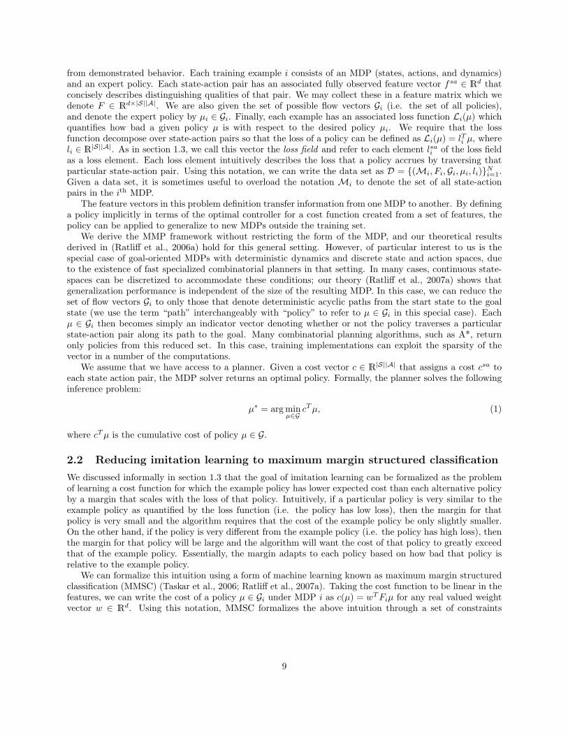
Figure 4: This figure visualizes the subgradient of a max over affine functions. Each affine function is denoted as a

dashed line, and the surface of the resulting convex function is delineated in bold. The subgradient a point w ∈ Wis simply the subgradient of the affine function that forms the surface at that point, shown here in red.

Additionally, since W can be any convex set, and since a step of fixed size αt may result in a point outsideof W, the update typically includes a projection back onto the feasible set:

wt+1 = PW [wt − αtgt] . (8)

The projection operator PW [·] can be approximate. The only requirement is that the projected point becloser to all other points in the convex setW than the original point was. This condition is typically expressedas

∀w′ ∈ W, ‖PW [w]− w′‖ ≤ ‖w − w′‖. (9)

By this definition, the projection has no effect on points already in the setW. Thus, this modified algorithmproceeds without projection until a step takes the hypothesis outside the feasible set. At that point, thehypothesis is projected back onto W. In our case, the set W is the set of weight vectors for which allcost elements in the provided examples are greater than a predefined positive constant. An approximateprojection operator can be implemented by iteratively projecting onto the most violated constraint. See(Ratliff et al., 2006a) for details.

2.3.2 Computing the subgradient for linear MMP

The terms wTFiµi and λ2 ‖w‖

2 are differentiable and, therefore, their unique subgradients are the gradientsFiµ and w, respectively. The term −minµ∈Gi{wTFiµ− lTi µ} is only slightly more complicated. The surfaceof this convex function is formed as a max over a set of affine functions. The subgradient at w is, therefore,the gradient of the affine function forming the surface at that point. We can find this surface affine functionsimply by solving the loss-augmented inference problem given in equation 3. Using that notation, the affinefunction forming the surface at w is (wTFi − lTi )µ∗i , and we know the subgradient of that function to beFiµ∗i .

5 Figure 4 visualizes the process of evaluating the subgradient of a max over affine functions.

to infinity. We often use αt = r√t+m

or αt = rt+m

in our experiments, where r is some nonnegative “learning rate” scalar and

m is a nonnegative integer specifying where along the progression the sequence starts. Intuitively, the steps reduce aggressivelyin the beginning but increasingly slow as time progresses. The parameter m, therefore, designates how quickly the step sizeshrinks in the beginning.

5There is a slight subtlety at points of non-differentiability. At such points, two or more affine functions intersect andthe loss-augmented inference problem has more than one solution (i.e. there are multiple optimal policies through the loss-augmented cost map). Since the subgradient algorithm requires only that one of the possible subgradients be followed at eachtime step, at these points we can choose any optimizer to construct a subgradient.

12

Using the above results, we can write the subgradient of the maximum margin planning objective givenin equation 7 as

∇R(w) =1N

N∑i=1

Fi(µi − µ∗i ) + λw

=1N

N∑i=1

Fi∆µ∗i + λw, (10)

where µ∗i is the solution to the loss-augmented inference problem from equation 3 for example i. We denote∆µ∗i = µi−µ∗i to emphasize that this component of the gradient is constructed by transforming the differencein frequency counts between the example policy µi and the loss-augmented policy µ∗i into the space of featuresusing the matrix Fi. This term singles out the feature vectors at states for which the frequency counts differsubstantially. If the example policy visits a particular state more frequently than the loss-augmented policy,the subgradient update rule will suggest a modification that will decrease the cost of that state. On theother hand, if the example policy visits a state less frequently, the update will want to increase the cost ofthat state.

The maximum margin planning algorithm, therefore, iterates the following update rule until convergence

wt+1 = PW [wt − αt (Fi(µi − µ∗i ) + λw)] . (11)

When both the environment and the policies are deterministic, the vector matrix product Fiµ can beimplemented efficiently using sparse multiplication. For instance, many of our experiments use the A*algorithm to find an optimal deterministic policy (i.e. a path) through the environment. We compute theproduct Fiµ simply by accumulating the feature vectors encountered while traversing the path representedby µ.

Optimal planning can be computationally infeasible for many practical problems, forcing the use of ap-proximate planners both during training and at runtime. Optimization in these cases is only approximate,but in (Ratliff et al., 2007a) we argue that the subgradient method holds certain robustness properties inthis situation. That paper, and later (Munoz et al., 2008) and (Munoz et al., 2009), demonstrate that thesubgradient method and its functional gradient generalizations perform well on large scale LADAR classifi-cation problems that require approximate inference. Additionally, (Kulesza & Pereira, 2008) demonstratesthat training with approximate inference implemented using an LP relaxation both works well in practiceand facilitates a characterization of approximate convergence.

3 Nonlinear techniques for optimization

In section 2, we introduced a class of algorithms based on the subgradient method for learning linear modelsunder MMP. This linear setting is understood quite well; we have a number of theoretical results analyzingthe convergence and generalization properties of these algorithms. However, applying these algorithms inpractice can be difficult when good features are not clear from the outset. Theoretical analyses in machinelearning often make statements that compare the performance of the learner to the performance of thebest hypothesis. Unfortunately, when the hypothesis class is too restrictive, such settings can be meaningless in terms of the overall performance of the learner. Moreover, designing a linear hypothesis class thatis sufficiently expressive to contain good hypotheses can be hard in real-world problems. Engineering asufficiently expressive set of features for a linear hypothesis class in robotics can be one of the most difficultand time consuming components of designing a high-performance system.

In both this section and section 4, we address this problem by utilizing nonlinear hypothesis spaces.Rather than assuming an expressive feature set, we learning the features as a function of a more basicfeatures during training. The algorithms that result train nonlinear hypotheses that perform well even whenthe original features are not expressive enough to form sufficient linear hypotheses.

We start this section with a review of boosting as functional gradient descent (Mason et al., 1999), and

13

then generalize that setting to derive a novel class of exponentiated functional gradient descent algorithms.Section 4 applies these algorithms to MMP. As we discuss in that section, the functions contained in theresulting hypothesis class better adhere to our prior beliefs about functions in planning applications.

3.1 Generalizing gradient descent to function spaces

We briefly review the argument presented in (Ratliff et al., 2006b) for generalizing gradient descent tothe functional setting. That argument follows and slightly generalizes the argument originally providedby (Mason et al., 1999), demonstrating that boosting algorithms can be viewed as a form of gradientdescent in function space. Let L2 be the space of square integrable functions. Consider objective functionalsF : L2 → R defined over functions c ∈ L2 as a sum of terms φ : R → R, each of which depend on c(·)through its evaluation at some xi. These objective functionals can be written as:

F [c] =k∑i=1

φ(c(xi)). (12)

Evaluation of a function is a linear operation which can be defined as the L2 inner product between thefunction c(·) and the Dirac delta function δx(·) centered at the point x in question. Specifically,

c(x) = 〈δx, c〉 =∫Xδx(x′)c(x′)dx′. (13)

As a linear functional, the gradient of the evaluation functional is simply given by

∇fc(x) = ∇f 〈δx, c〉 = δx. (14)

Here we denote the functional gradient by ∇f to distinguish it from the parametric gradient of Section 2.3.The functional gradient of objective functionals of the form given in equation 12 is therefore:

∇fF [c] =k∑i=1

∇fφ(c(xi)) =k∑i=1

φ′(c(xi))δxi . (15)

In the final expression, we use the common abbreviation φ′(c(x)) = dduφ(u)|c(x).

The expression defining the functional gradient in equation 15 is too abstract to use in practice. Thedelta functions provide only impulse information regarding how the current hypothesis function should beperturbed at a specific discrete set of points {xi}ki=1. To utilize these functional gradients we must firstproject them onto a predefined set of hypothesis functions H that we can use to build our model. We oftencall this set of hypothesis functions the direction set since they form the set of allowable direction vectorsthat can be used to navigate the function space. As we will see, the boosting algorithm finds the directionh∗ ∈ H which best correlates with the functional gradient g = ∇fF [c] defined by h∗ = arg maxh∈H 〈h, g〉.

For objective functionals of the form specified in equation 12, this inner product optimization can bewritten as:

h∗ = arg maxh∈H

⟨h,

k∑i=1

φ′(c(xi))δxi

⟩= arg max

h∈H

k∑i=1

〈h, φ′(c(xi))δxi〉 (16)

= arg maxh∈H

k∑i=1

φ′(c(xi))h(xi). (17)

It is often the case that this maximization problem can be implemented efficiently (though approximately)using traditional binary classification or regression algorithms from the machine learning literature. Forinstance, in the most common application of this algorithm, the direction set is defined as a set of binaryfunctions H ⊂ {h | h(x) ∈ {−1, 1}∀x ∈ X}. If we define αi = |φ′i(c(xi))| and yi = sign(φ′i(c(xi))), then the

14

Algorithm 3 Functional gradient intuition

1: procedure FunGrad( objective functional F [·], initial function h0, step size sequence {γt}∞t=1 )2: while not converged do3: Evaluate the functional gradient gt of the objective functional at the current hypothesis

ft = −∑t−1τ=0 γτhτ .

4: Find the element ht = h∗ ∈ H which best correlates with the functional gradient gt by maximizingeither equation 17 or equation 19.

5: Take a step in the negative of that direction forming ft+1 = ft − γtht = −∑tτ=0 γτhτ .

6: end while7: end procedure

optimization problem in equation 17 can be recast as:

h∗ = arg maxh∈H

k∑i=1

αiyih(xi). (18)

This is a weighted binary classification problem, and can be solved using any of a variety of classificationalgorithms.

Alternatively, as discussed in (Friedman, 1999a), we can re-define our correlation measure as a weightedleast squares classification problem. Using the same notation as above, we replace equation 18 with

h∗ = arg minh∈H

k∑i=1

αi(yi − h(xi))2. (19)

There are a number of reasons why this correlation measure may be preferred over the inner product givenin equation 17. Friedman notes that the estimator is consistent (Friedman, 1999a). Some straightforwardcalculations show that we can rewrite this correlation measure as:

arg minh∈H

k∑i=1

αi(yi − h(xi))2 = arg maxh∈H

(k∑i=1

φ′i(c(xi))h(xi)−12

k∑i=1

|φ′i(c(xi))|h(xi)2

). (20)

This expression is essentially the same as equation 17, except there is an additional regularization type termwhich penalizes the size of the function h at each point xi proportionally to how large the weight on thecorresponding gradient component is at that point.

For the purposes of finding the most correlated search direction, this new correlation definition is equiv-alent to that defined in equation 17 when the direction set is the set of all classification algorithms (i.e.h(x) ∈ {−1, 1}, ∀x). Indeed, the quadratic second term of the argmax on the right hand side of equation 20is constant with respect to h because h(x)2 = 1 since h(x) itself is either 1 or −1. However, for more generaldirection sets, this modified definition of correlation constrains the size of functions. The original linearMMP algorithms suffered from a sensitivity to the relative scaling of its features, a problem common to mar-gin based learning formulations including alternative IRL formulations as discussed in (Neu & Szepesvari,2007).6 Section 4.3 demonstrates a solution to this problem that arises naturally from this regression-basedcorrelation measure when used with a hypothesis space of linear functions. The functional gradient descentalgorithm proceeds as presented in Algorithm 3.

Operationally, a functional gradient can be viewed as a regression data set. This data set suggests whereand how strongly the function should be increased or decreased at a collection of points in the feature space.For instance, let D = {fi, yi}Ni=1 be such a data set. Each yi is a real number suggesting how strongly the

6Intuitively, since we typically require the weight vector to lie within a Euclidean ball, a feature whose range is 10 timeslarger than another will likely dominate the hypothesis since a tiny weight on that feature can produce the same amount ofcost variation as a large weight on the other.

15

Figure 5: This figure shows a pictorial representation of the action of a functional gradient data set. The left plot

shows the original function in gray along with a functional gradient data set indicated where and to what extent

the function should be modified. The second plot includes a nonlinear regressor that generalizes from that data set

to the rest of the domain. Finally, the right-most image shows the result of taking a functional gradient step: the

nonlinear regressor in the second plot is simply added to the original function effectively implementing the discrete

set of suggested modifications.

function should be modified. If yi is strongly positive, then this data point suggests a strong increase inthe function at fi. Alternatively, if yi is strongly negative, then the function should be strong decreasedat that point. Moreover, if yi is zero, or close to zero, the data point indicates that the function shouldnot be modified at all. Black box regression algorithms implement these suggestions and return to us atangible function that we can add to our hypothesis. Figure 5 demonstrates pictorially the intuitive affect offunctional gradient modification. On the left is a plot of the original function with the functional gradientsuggestions superimposed. Implementationally, these modifications result in the figure on the right.

Unfortunately, it is difficult to apply functional gradient descent directly to optimizing the maximummargin planning objective as many planning algorithms (e.g. A*) require the costs to be positive. In thelinear case, we satisfied the positivity constraints using an approximate projection step (Ratliff et al., 2006a)which iteratively projected onto the most violated constraint. It is more difficult, however, to apply sucha projection in the functional setting. In prior work (Ratliff et al., 2006b), we developed a technique thatutilized the linear MMP algorithm in the inner loop of the functional gradient algorithm to ensure adherenceto the positivity constraints. That algorithm, however, is both more difficult to implement and tends toconverge more slowly in practice.

In the next few sections, we develop an alternative approach to utilizing functional gradient which ensuresthat the learned function is positive everywhere. The algorithm, exponentiated functional gradient descent,is a generalization of exponentiated gradient descent to function spaces. Section 3.2 derives the exponenti-ated functional gradient descent algorithm by analogy to the parametric variant, and section 4 utilizes thisalgorithm within the context of MMP and derives the LEARCH framework.

3.2 Generalizing exponentiated gradient descent to function spaces

In this section, we use the same intuition that brought the finite-dimensional gradient descent algorithm tothe functional setting in section 3.1 to additionally generalize the finite-dimensional exponentiated gradientdescent algorithm. We prove that the resulting update in function space has positive inner product with thenegative functional gradient.

3.2.1 Exponentiated functional gradient descent

We can characterize the traditional Euclidean gradient descent update rule as a minimization problem. Atour current hypothesis wt, we create a linear approximation to the function (in the case of convex functions,this approximation is also a lower bound), and we minimize the approximation while regularizing back toward

16

wt. Mathematically, we write this as

wt+1 = arg minw∈W

f(wt) + gTt (w − wt) +λt2‖w − wt‖2, (21)

where gt = ∇f(wt) is the gradient (or subgradient) at wt. Analytically solving for the minimizer by settingthe gradient of the expression to zero derives the Euclidean gradient descent rule: wt+1 = wt − αtgt withstep size αt = 1/λt. Thus, the gradient descent rule naturally encourages solutions that have a small normin the sense of ‖ · ‖2 (see (Zinkevich, 2003)). A similar procedure derives the update rule for exponentiatedgradient descent as well. Replacing the Euclidean regularization term in equation 21 with an unnormalizedKL-divergence regularization of the form uKL(w,wt) =

∑j w

j log wj

wjt−∑j w

j +∑j w

jt and analytically

solving for the minimizer results in the exponentiated gradient update rule (Kivinen & Warmuth, 1997):

wt+1 = wte−αtgt = e−

Ptτ=0 ατgτ (22)

= eut (23)

where {αt}∞t=1 is a sequence of step sizes (sometimes called learning rates). For simplicity, we assume inwhat follows that w0 is the vector of all ones, i.e. w0 = ez where z is the zero vector. This assumption isnot necessary, but it lightens the notation and clarifies the argument.

In the final expression of equation 22, we denote ut = −∑τ ατgτ in order to point out the relationship

to the Euclidean gradient descent algorithm. The quantity ut is the hypothesis that would result from anobjective function whose gradients were gt at each xt. The only difference between the gradient descentalgorithm and the exponentiated gradient descent algorithm is that in the gradient descent algorithm wesimply evaluate the objective and its gradient using ut, while in the exponentiated gradient algorithm,since the objective is a function of vectors from only the positive orthant, we first exponentiate this vectorwt = eut before evaluating the objective and its gradient. Essentially, the exponentiated gradient updaterule is equivalent to the gradient descent update rule, except we exponentiate the result before using it.

In addition to the immediate benefit of only positive solutions, the key benefit enjoyed by the exponen-tiated gradient algorithm is a robustness to large numbers of potentially irrelevant features. In particular,powerful results (Kivinen & Warmuth, 1997; Cesa-Bianchi & Lugosi, 2006) demonstrate that the exponen-tiated gradient algorithm is closely related to the growing body of work in the signal processing communityon sparsity and ‖ · ‖1 regularized regression. (Tropp, 2004; Donoho & Elad, 2003) Exponentiated gradientachieves this by rapidly increasing the weight on a few important predictors while quickly decreasing theweights on a bulk of irrelevant features. The unnormalized KL prior from which it is derived encouragessolutions with a few large values and a larger number of smaller values. In the functional setting, the weightsare analogous to the hypothesized function evaluated at particular locations in feature space. We believe thisform of regularization– or prior, taking a Bayesian view– is natural for many planning problems in roboticswhere there is a very large dynamic range in the kind of costs to be expected.

This work generalizes the connection between these two optimization algorithms to the functional set-ting. A formal derivation of the resulting algorithm is quite technical and beyond the scope of this paper.The algorithm, however, is straightforward and analogous to the finite-dimensional setting. We derive thisalgorithm informally in what follows.

In functional gradient descent, we evaluate the functional gradient of the objective function, find thesearch direction from a predefined set of hypothesis functions that correlates best with the functional gradient,and take a step in the negative of that direction. In the exponentiated functional gradient algorithm wewill essentially perform the same update (take a step in the negative direction of the projected functionalgradient), but before evaluating the objective function or the functional gradient we will exponentiate thecurrent hypothesis.

Explicitly, the exponentiated functional gradient descent algorithm dictates the procedure presented inAlgorithm 4.

17

Algorithm 4 Exponentiated functional gradient intuition

1: procedure ExpFunGrad( objective functional F [·], initial function h0 )2: while not converged do3: Evaluate the functional gradient gt of the objective functional at the current hypothesis

ft = e−Pt−1τ=0 γτhτ .

4: Find the element ht = h∗ ∈ H which best correlates with the functional gradient gt by maximizingeither equation 17 or equation 19.

5: Take a step in the negative of that direction forming ft+1 = fte−γtht = e−

Ptτ=0 γτhτ .

6: end while7: end procedure

3.2.2 Theoretical results

We show here that when the functional gradient can be represented explicitly the exponentiated functionalgradient descent algorithm produces a modification to the hypothesis that has a positive inner product withnegative functional gradient. Therefore, on each iteration, there always exists a finite step length intervalfor which the algorithm necessarily decreases the desired objective while preserving the natural sparsity anddynamic range of exponentiated costs.

Let gt(x) be the functional gradient of a functional at hypothesis ft(x). Under the exponentiated func-tional gradient algorithm, ft(x) = eht(x) for some log-hypothesis ht(x). Thus, we need only consider positivehypotheses: f(x) > 0 for all x. Our update is of the form ft+1(x) = ft(x)e−λtg(x), where λt > 0 is a positivestep size. Therefore, we can write our update offset vector as

vt(x) = ft+1(x)− ft(x) = f(x)e−λg(x) − f(x)

= ft(x)(e−λgt(x) − 1

).

We suppress the dependence on t in what follows for convenience.

Theorem 3.1: The update direction v(x) has positive inner product with the negative gradient. Specifically,

−∫Xg(x)v(x)dx =

∫Xg(x)f(x)

(1− e−λg(x)

)dx > 0.

Proof. We first note that φ(u) = 1u

(eu − 1) is continuous and everywhere positive since u and eu − 1 alwayshave the same sign.7 We can rewrite our expression asZ

Xg(x)f(x)

“1− e−λg(x)

”dx =

ZXg(x)f(x)

“λg(x)φ(−λg(x))

”dx

= λ

ZXg(x)2f(x)φ(−λg(x))dx.

The integrand is everywhere nonnegative, and when our functional gradient is not the zero function, there existmeasurable regions over which the integrand is strictly positive. Therefore, −

RX g(x)v(x)dx > 0. 2

The next section derives the LEARCH class of algorithms by applying our exponentiated functionalgradient descent algorithm to the maximum margin planning framework.

7Technically φ(u) has a singularity at u = 0. However, since the left and right limits at that point both equal 1, withoutloss of generality we can define φ(0) = 1 to attain a continuous function.

18

4 Exponentiated functional gradient descent formaximum margin planning

Initial work into MMP focused on the linear setting in which the cost function is assumed to be a linearfunction of a predefined set of features. The optimization algorithms in this setting are just a simple varianton parametric gradient descent; unfortunately, while the linear setting is more easily understood theoretically(see (Ratliff et al., 2006a; Ratliff et al., 2007a)), feature extraction for linear models is often difficult.

We are now prepared to generalize the maximum margin planning framework. In the functional setting,the MMP objective takes on essentially the same form as equation 7, but with each policy cost term wTFiµreplaced by the more general term

∑(s,a)∈Mi

c(fsai )µsa:

R[c] =1N

N∑i=1

∑(s,a)∈Mi

c(fsai )µsai − minµ∈Gi{∑

(s,a)∈Mi

(c(fsai )− lsai )µsa}

. (24)

As before, this functional sums over all examples the difference between the cumulative cost of the ith

example policy∑

(s,a)∈Mic(fsai )µsai and the cumulative cost of the (loss-augmented) minimum cost policy

minµ∈Gi{∑

(s,a)∈Mi(c(fsai ) − lsai )µsa}. Since the example policy is a valid policy, the minimum cost policy

will always be smaller. Each example’s objective term (the ith term) is, therefore, always nonnegative. Itrepresents the degree to which the example policy is suboptimal under the hypothesized cost function.

The linear setting typically includes an explicit L2 regularization term; we remove the regularization termin this expression to simplify the requirements on the corresponding optimization algorithm. Boosting-typefunctional gradient descent procedures often admit regularization path arguments of the type discussed in(Rosset et al., 2004). These arguments state that the number of boosting steps executed determines theeffective size or complexity of the model class under consideration. Early stopping, therefore, plays a similarrole to regularization, and we need not explicitly represent the regularization term.8

This section discusses the algorithm that arises when the exponentiated functional gradient decent algo-rithm we presented in section 3.2 is applied to optimizing this functional. We demonstrate that the resultingclass of algorithms is that discussed intuitively in section 1.2. Moreover, section 4.3 presents a specificinstantiation of the class that has a similar efficient representation to the original linear MMP algorithm.However, we demonstrate experimentally that the algorithm can significantly outperform the older variant.

4.1 General setting

Using the tools described in section 3.1, we can derive the L2 functional gradient of the maximum marginplanning objective functional (see equation 24) as

∇fR[c] =1N

N∑i=1

∑(s,a)∈Mi

µsai δfsai −∑

(s,a)∈Mi

µ∗isaδfsai

. (25)

In this expression, we denote µ∗i = arg minµ∈Gi{∑

(s,a)∈Mi(c(fsai )−lsai )µsa}; we call this quantity the optimal

loss-augmented policy.The functional gradient has the same form as that considered in section 3.1: it is a weighted sum of

delta (impulse) functions∑j γjδxj . In this case, magnitude of a given weight is determined by the frequency

count at that state-action pair, and the sign of the weight is determined by whether it comes from theloss-augmented policy or the example policy.

8Additionally, boosting relies implicitly on the class of weak learning algorithms to induce generalization and limit hypothesiscomplexity. Strongly regularized weak learners induce slower complexity growth.

19

Algorithm 5 Exponentiated functional gradient descent for maximum margin planning

1: procedure LEARCH( training data {(Mi, ξi)}Ni=1, loss function li, feature function fi )2: Initialize log-costmap to zero: s0 : Rd → R, s0 = 03: for t = 0, . . . , T − 1 do4: Initialize the data set to empty: D = ∅5: for i = 1, . . . , N do6: Compute the loss-augmented costmap cli = est(Fi) − lTi and find the minimum cost loss-

augmented path through it µ∗i = arg minµ∈Gi cliµ

7: Generate positive and negative examples: ∀(s, a) ∈Mi,D = {D, (fsai , 1, µ∗isa), (fsai ,−1, µisa)}

8: end for9: Train a regressor or classifier on the collected data set D to get ht

10: Update the log-hypothesis st+1 = st + αtht11: end for12: return Final costmap esT

13: end procedure

4.2 Intuition

Algorithm 5 details the LEARCH algorithm. This listing demonstrates explicitly how to implement theoperation of finding a direction function that correlates well with the functional gradient. Intuitively, thefunctional gradient can be viewed as a weighted classification or regression data set, where weights comefrom the magnitude of the delta function coefficients in the gradient term, and the label comes from the signof these coefficients.

At each iteration, the exponentiated functional gradient algorithm starts by finding a direction function,defined over the feature space, that correlates well with the negative functional gradient. Intuitively, thismeans that the function is positive in regions of the feature space where there are many positive deltafunctions (in the negative gradient) and negative in regions where there are many negative delta functions.It then adds this direction function to the log of the previously hypothesized cost function with a small scalarstep size αt. (The step size may decrease toward zero over time as discussed in section 2.3.) Adding thedirection function to the cost function effectively increases and decrease the hypothesis as dictated by theimpulse signals found in the negative functional gradient. Finally, the algorithm exponentiates the modifiedlog-hypothesis to arrive at a valid positive cost function.

Intuitively, the negative functional gradient places negative impulses at feature vectors found along state-action pairs seen while executing the example policy so that the cost function is decreased in those regions.Conversely, it places positive impulses at feature vectors found along state-action pairs encountered whileexecuting the loss-augmented policy so that the cost function is increased in those regions. In both cases,the magnitude of each impulse is proportional to the frequency with which the relevant policy traversesthe state-action pair. If the distribution of feature vectors seen by both the example policy and the loss-augmented policy coincide, then the positive and negative impulses cancel resulting in no net suggestedupdate. However, if the distributions diverge, then the algorithm will decrease the cost function in regionsof the feature space where the example policy dominates and increase the cost function in regions where theloss-augmented policy (erroneously) dominates.

We have already seen this algorithm in section 1.3, where we motivated it from a practical standpointfor the specific case of deterministic planning. In some problems, we do not require the cost function to bepositive everywhere. For those cases, we may simply apply the more traditional non-exponentiated variant(i.e. gradient boosting (Mason et al., 1999)). Section 5 describes experiments using both exponentiated andnon-exponentiated variants of the algorithm on two imitation learning problems from the field of robotics.

20

4.3 A log-linear variant

The mathematical form of the cost function learned under the LEARCH framework is dictated by the choiceof the regressor or classifier used to implement the functional gradient projection step. In this section, welook at the simplest case of applying linear regression to approximate the functional gradient– this oftenrepresents a simple, efficient, and effective starting point even when additional non-linear functional gradientapproximations are to be applied.

Since a linear combination of linear functions is also a linear function, the final cost function has anefficient log-linear representation

fk(x) = ePkt=1 αtht(x) = e

Pki=1 αtu

Tt x = ew

Tt x,

where wk =∑t αtut. Moreover, exponentiating the linear function creates a hypothesis space of cost func-

tions with substantially higher dynamic ranges for a given set of features than our original linear alternativewhich we presented in section 2.3. We find that this log-linear variant demonstrates empirically superiorperformance (Figure 7).

4.3.1 Deriving the log-linear variant

We derive this variant of LEARCH simply by choosing a set of linear functions h(x) = wTx as the directionset. The following theorem presents the update rule resulting under the least-squares functional gradientcorrelation estimator.

Theorem 4.1: Let wt be the hypothesized weight vector at the tth time step. Then the update rule withstep size ηt under the least-squares correlation estimator of equation 19 takes the form wt+1 = wt− ηtC−1

t gtwhere gt is the parametric Euclidean gradient given in equation 10 and Ct =

∑Ni=1 Fi diag (µi + µ∗i ) Fi

T .

Specifically, our hypothesis at time T takes the form cTMi(µ) = e−(PT

t=1 ηtC−1t gt)TFiµ.

Proof. We prove the theorem for the general objective discussed in section 3.1. Applying this result to equation24 completes the proof. Given a linear hypothesis space, the least-squares functional gradient correlation estimatorinduces the following quadratic objective function:*

hw,

kXj=1

αjxj

+− 1

2

kXj=1

|αj |hw(xj)2 = wT

kXj=1

αjxj −1

2wT

kXj=1

|αj |xjxTj

!w.

Since this expression is quadratic, we can solve for the optimal update direction by setting its gradient to zero. Doingso gives w∗ = C−1Pk

j=1 αjxj , where C =Pkj=1 |αj |xjx

Tj . Since each αj is implicitly a function of w, C is also a

function of w, and we can therefore view C as an adaptive whitening matrix. 2

One may view this modified search direction as the parametric gradient taken under the Riemannianmetric Ct. Under the MMP functional, this Riemannian metric adapts to the current combined distributionof feature vectors included by the example and loss-augmented policies. Importantly, using the modifiedcorrelation criterion removes the feature scaling problem discussed in (Neu & Szepesvari, 2007) referencedin section 3.1.

4.3.2 Log-linear LEARCH vs linear MMP

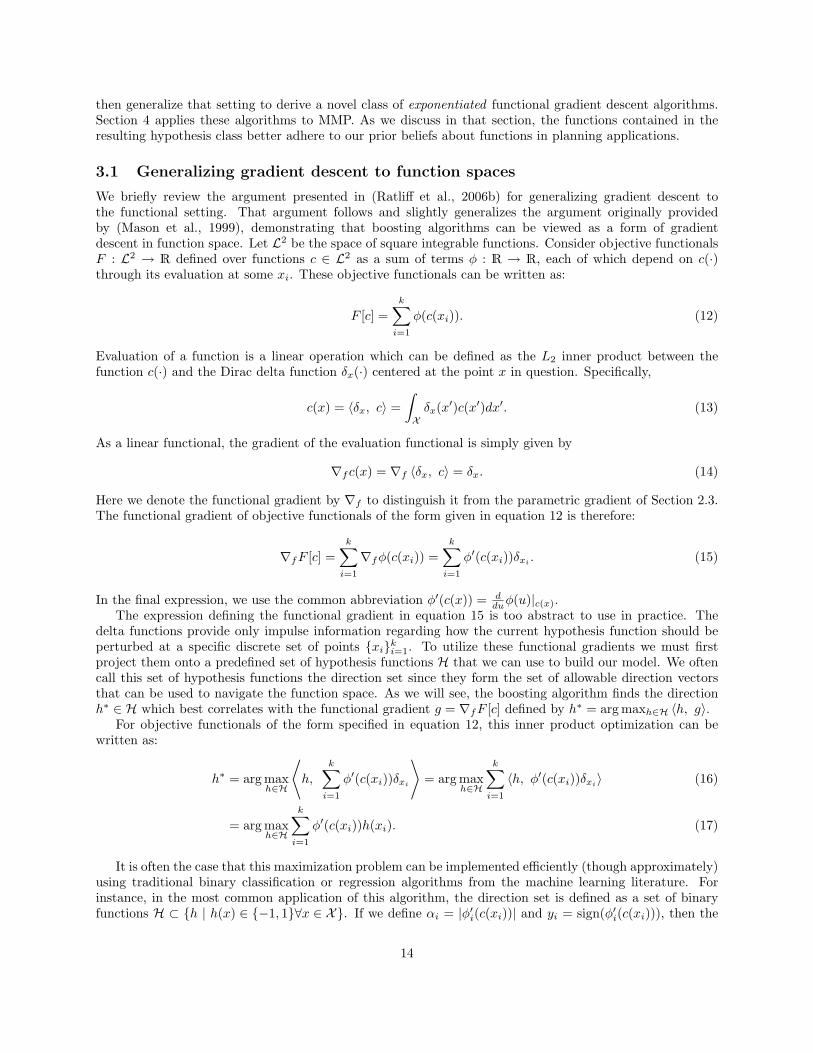
Figure 6 depicts a straightforward example of where the log-linear LEARCH algorithm is able to substantiallyoutperform linear MMP. The leftmost panel shows an overhead satellite image depicting a test region, heldout from the training set, which we use to evaluate both algorithms. The feature set for this problemconsisted solely of Gaussian smoothings of the original grayscale overhead satellite images. We purposefullychose these features to be simple to emphasize the performance differences. The linear MMP algorithmfailed to generalize the expert’s behavior to the test region (rightmost panel). The best linear combinationof features found by linear MMP defined a cost function with very small dynamic range and implemented anaıve minimum distance policy. However, when allowed to exponentiated the linear combination of features,

21

Figure 6: The LEARCH framework suggests a log-linear algorithm which can be used as an alternative to linear

maximum margin planning (MMP). The cost functions in the log-linear variant’s hypothesis space generally achieve

higher dynamic ranges for a given feature set and, therefore, tend to show empirically superior performance. This

figure compares the two algorithms on a simple application using the holdout region shown in the leftmost panel.

The rightmost panel shows the planning performance on the best linear combination of features achieved by linear

MMP, and the center panel shows best exponentiated linear combination of features found by the log-linear LEARCH

algorithm. The log-linear algorithm generalizes the expert’s behavior well and clearly outperforms linear MMP on

this problem.

within 6 iterations, the log-linear LEARCH algorithm (center panel) successfully converged to an expressivecost function that generalized the behavior well.

Additionally, figure 7 depicts the difference in validation performance between log-linear LEARCH andlinear MMP on a more realistic problem using a stronger feature set, including color class, multi-spectral,and texture features. For this experiment, we optimized the linear MMP objective using functional gradientboosting of linear hypotheses and satisfied cost-positivity constraints by truncating the costs to a minimumvalue. Log-linear LEARCH significantly outperforms linear MMP on this problem because of the increaseddynamic range in its hypothesis space.

4.4 Implementation with different planners

At a high level, the implementation of LEARCH simply follows the procedure described in Algorithm 5.However, in practice there are additional details related to the choice of algorithms for regression andplanning, as well as the exact form and quality of human training input available. Often, these details arenot free parameters, but rather are constraints imposed by a specific problem or platform.

LEARCH requires determining the frequency counts for each state for both the example plan and planunder the current cost function. For some planners, this is relatively straightforward; for example, witha basic A* planner, each state along each path is visited once. However, for other planners, additionalbookkeeping is required. Since the goal of this work is to learn the proper cost function for a specificplanner, planner details must be taken into account.

In motion planning, planners often apply a configuration space expansion to an input cost map beforegenerating a plan, to account for the physical dimensions of a robot. When such an expansion does takeplace, it must also be taken into account by LEARCH; the cost function must be learned such that afterexpansion, the desired behavior is reproduced. For example, if the planner takes the average cost of all stateswithin a window around the current state, then the frequency count of all the states within the same windowmust be incremented. If the expansion applies different weightings to different states, then this weightingmust also be applied when incrementing the frequency counts. Finally, if the expansion applies a weightingto a set of states that is a function of the underlying cost values (for example, the max of the set) this sameweighting must still be applied; however, in this case LEARCH will no longer be convex.

While the MMP framework allows for continuous state spaces, LEARCH requires discrete examples.In practice, continuous state spaces can be handled with a sufficiently high-resolution discretization. Thismay in turn require non-unit changes to frequency counts, regardless of an expansion. For example the

22

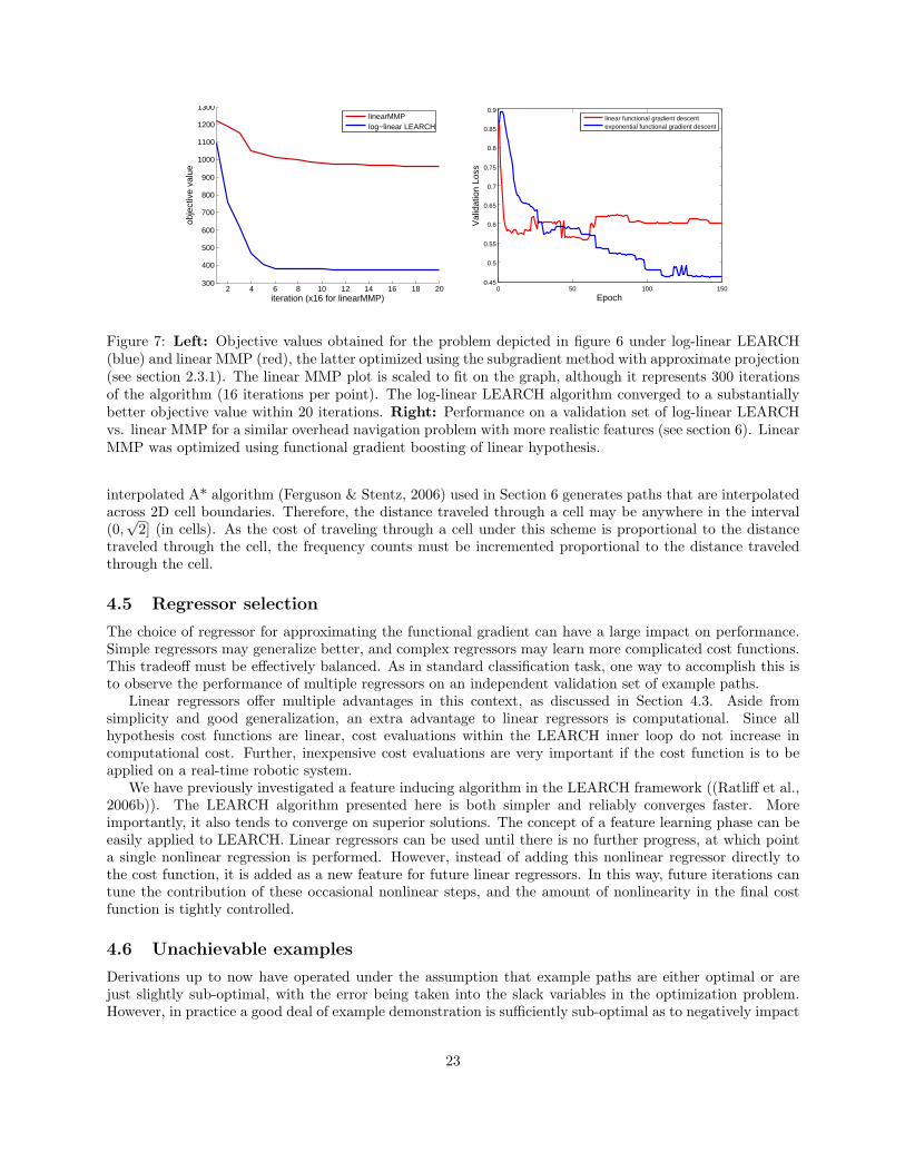
2 4 6 8 10 12 14 16 18 20300

400

500

600

700

800

900

1000

1100

1200

1300

iteration (x16 for linearMMP)

obje

ctiv

e va

lue

linearMMPlog−linear LEARCH

0 50 100 1500.45

0.5

0.55

0.6

0.65

0.7

0.75

0.8

0.85

0.9

Epoch

Val

idat

ion

Loss

linear functional gradient descentexponential functional gradient descent

Figure 7: Left: Objective values obtained for the problem depicted in figure 6 under log-linear LEARCH(blue) and linear MMP (red), the latter optimized using the subgradient method with approximate projection(see section 2.3.1). The linear MMP plot is scaled to fit on the graph, although it represents 300 iterationsof the algorithm (16 iterations per point). The log-linear LEARCH algorithm converged to a substantiallybetter objective value within 20 iterations. Right: Performance on a validation set of log-linear LEARCHvs. linear MMP for a similar overhead navigation problem with more realistic features (see section 6). LinearMMP was optimized using functional gradient boosting of linear hypothesis.

interpolated A* algorithm (Ferguson & Stentz, 2006) used in Section 6 generates paths that are interpolatedacross 2D cell boundaries. Therefore, the distance traveled through a cell may be anywhere in the interval(0,√

2] (in cells). As the cost of traveling through a cell under this scheme is proportional to the distancetraveled through the cell, the frequency counts must be incremented proportional to the distance traveledthrough the cell.

4.5 Regressor selection

The choice of regressor for approximating the functional gradient can have a large impact on performance.Simple regressors may generalize better, and complex regressors may learn more complicated cost functions.This tradeoff must be effectively balanced. As in standard classification task, one way to accomplish this isto observe the performance of multiple regressors on an independent validation set of example paths.

Linear regressors offer multiple advantages in this context, as discussed in Section 4.3. Aside fromsimplicity and good generalization, an extra advantage to linear regressors is computational. Since allhypothesis cost functions are linear, cost evaluations within the LEARCH inner loop do not increase incomputational cost. Further, inexpensive cost evaluations are very important if the cost function is to beapplied on a real-time robotic system.

We have previously investigated a feature inducing algorithm in the LEARCH framework ((Ratliff et al.,2006b)). The LEARCH algorithm presented here is both simpler and reliably converges faster. Moreimportantly, it also tends to converge on superior solutions. The concept of a feature learning phase can beeasily applied to LEARCH. Linear regressors can be used until there is no further progress, at which pointa single nonlinear regression is performed. However, instead of adding this nonlinear regressor directly tothe cost function, it is added as a new feature for future linear regressors. In this way, future iterations cantune the contribution of these occasional nonlinear steps, and the amount of nonlinearity in the final costfunction is tightly controlled.

4.6 Unachievable examples

Derivations up to now have operated under the assumption that example paths are either optimal or arejust slightly sub-optimal, with the error being taken into the slack variables in the optimization problem.However, in practice a good deal of example demonstration is sufficiently sub-optimal as to negatively impact

23

Figure 8: Left:The red path is an unachievable example path, as it will be less expensive under any costfunction to cut more directly across the grass. Center Left: With standard weighting, the unachievableexample forces down the cost of grass, and prevents the blue example from being achieved. Center Right:Normalized weighting prevents this bias, and the blue path is achieved Right: The ratio of the normalizedto the standard costmap. The cost of grass is higher in the normalized map.

generalization. The next two sub-sections present techniques that can provide increased robustness to sub-optimal example behavior.

In practice, it is often possible to generate an example path such that no consistent cost metric in thehypothesis space will make the example optimal. Figure 8 provides a simple example of such a case. The redexample path takes a very wide berth around some obstacles. The features of all the terrain the path travelsthrough are essentially the same, and so will have similar cost. If the spacing the path gives the obstaclesis greater than the size of the configuration space expansion of the planner, no cost function exists underwhich the example is optimal; it will always be lower cost to cut more directly around the obstacle.

Such a case occurs in a small way on a high percentage of human provided examples. People rarelyexhibit perfectly optimal behavior, and often generate examples that are a few percent longer than necessary.Further, a limited set of features and planner limitations mean that the path a human truly considers to beoptimal may not be achievable using the planning system and features available to learn with.

It is instructive to observe what happens to the functional gradient with an unachievable example.Imagine an environment where all states are described by the identical feature vector f ′. Under this scenario,equation 25 reduces to

∇fR[c] =

{1N

∑Ni=1

(∑(s,a)∈Mi

µsai −∑

(s,a)∈Miµ∗i

sa)

if f = f ′

0 if f 6= f ′

the functional gradient depends only on the lengths of the example and current plan, under any cost function.If the paths are not of equal length, then the optimization will never be satisfied. Specifically, if the examplepath is too long, there will always be an extra component of the gradient that attempts to lower costs.Intuitively, an unachievable example implies that certain costs should be 0, a condition that is not allowedby many planners. By continually implying that certain costs should be lowered, unachievable examples cancounteract the effect of other (achievable) paths, resulting in cost functions with less dynamic range, andthat result in poorer performance (see Figure 8).

This effect can be counteracted with a small modification to the procedure of approximating the functionalgradient proposed in (Silver et al., 2008)9. Simplifying notation, define the negative gradient vector as

−∇fF [c] = U∗ − Ue

Where U∗ and Ue are the frequency counts of the planned and example paths, respectively.Now consider a new gradient vector that looks at the normalized feature counts

−Gnorm =U∗||U∗||

− Ue||Ue||

(26)

9(Silver et al., 2008) propose an L1 normalization, as opposed to the L2 normalization derived above, with empiricallysimilar results

24

In the special case mentioned above, this new gradient would be satisfied with the cost function as is. It canbe shown that in all other cases, the new gradient still points in the correct direction.

Theorem 4.2: The normalized functional gradient Gnorm has a positive inner product with the unnormal-ized functional gradient, except when the frequency counts are perfectly correlated.

Proof.

〈−∇fF [c],−Gnorm〉 = 〈U∗ − Ue,U∗||U∗||

− Ue||Ue||

〉 =||U∗||2 − 〈U∗, Ue〉

||U∗||+||Ue||2 − 〈U∗, Ue〉

||Ue||

= ||U∗||+ ||Ue|| − 〈U∗, Ue〉(1

||U∗||+

1

||Ue||)

By the Cauchy-Schwarz inequality, we can bound 〈U∗, Ue〉 with ||U∗||||Ue||

||U∗||+ ||Ue|| − 〈U∗, Ue〉(1

||U∗||+

1

||Ue||) ≥ ||U∗||+ ||Ue|| − ||U∗||||Ue||(

1

||U∗||+

1

||Ue||) = 0

When 〈U∗, Ue〉 is not tight against the upper bound

〈−∇fF [c],−Gnorm〉 > 0

2

It is worth noting from the proof that 〈−∇fF [c],−Gnorm〉 is negatively correlated with 〈U∗, Ue〉. Thatis, when the example and planned paths pass through states with very different features, the normalizedand unnormalized functional gradients are very similar. As the features becomes more similar, the gradientsdiverge; when the features become identical, the gradients become orthogonal.

In terms of projecting the new gradient −Gnorm onto the set of hypothesis functions, equation 17 becomes

h∗ = arg maxh∈H

∑yi>0

αih(xi)√∑yi>0

α2i

−

∑yi<0

αih(xi)√∑yi<0

α2i

(27)

with a similar normalization for equation 19.The net effect of this normalization is to perform a more balanced classification or regression. As long

as the learner can still separate between examples for which the cost should be increased and decreased, thenormalized result will have the same effect. When the learner can no longer distinguish between the classes,the gradient will shrink and eventually become zero, as opposed to simply moving in the direction of themore populous class (see Figure 8).

4.7 Alternate constraints from example behavior

Often, individual examples are achievable, but inconsistent with other examples. When examples are incon-sistent it is often by a small amount, due to the inherent noise in human provided example behavior. Forexample, in constrained environments human examples sometimes give obstacles too a narrow berth (withrespect to the expansion of the planner), incorrectly implying the obstacle should be lower cost.

One approach to increasing robustness to this form of noise is to slightly redefine the constraints on costfunctions implied by each example. Instead of considering an example path as indicative of the exact optimalplan, it can be considered instead as the approximately optimal plan. That is, instead of trying to enforcethe constraint that no path is lower cost then the example, enforce the constraint that no path is lower costthan the lowest cost path that is close to the example. For example, for planning in a state space of Rn, thisalternate formulation would enforce the constraint that no path is lower cost than the lowest cost path thatexists completely within a corridor (of some specified width) around the example. Formally, the functional

25

gradient becomes

∇fR[c] =1N

N∑i=1

∑(s,a)∈Mi

µε∗sai δfsai −∑

(s,a)∈Mi

µ∗isaδfsai

. (28)

where µε∗i is defined as

µε∗i = arg minµ∈Gµi,εi

{∑

(s,a)∈Mi

(c(fsai ))µsa}

and Gµi,εi is the set of all paths close to the example. Gµi,εi can be defined in any consistent way; onenatural choice is to define Gµi,εi as the set of paths with sufficiently small loss. The result of this new setof constraints is that the gradient is not affected by small details; In effect, the example has been smoothedto reduce noise. To prevent oversmoothing, the optimal threshold for defining Gµi,εi can be determined bymaximizing validation set performance.

One downside of this new formulation is that the objective functional is no longer convex (Since µε∗ialso contains an arg min). While it is certainly possible to construct cases with a single path that resultin convergence to a poor cost function, empirical observation has shown that as long as more than a fewexamples are used, all the local minima achieved are quite satisfactory (Silver et al., 2008).

More complicated versions of this alternative formulation are also possible. For instance, instead of afixed width corridor along an example path, a specified variable width corridor could be used. This wouldallow examples with high importance at some sections (at pinch points) and low importance elsewhere.Another version of this formulation would involve multiple disjoint corridors. This could be used if an expertbelieved there were two different but equally desirable “best” behaviors from start to goal.

5 Case study: Multiclass classification

In this section, we demonstrate LEARCH on two multiclass classification problems: footstep prediction andgrasp prediction. These experiments used single-hidden-layer neural networks to implement the functionalgradient approximation step in line 9 of algorithm 5.10

5.1 Footstep prediction

Recent work has demonstrated that decomposing legged locomotion into separate footstep planners andexecution controllers is an effective strategy for many problems (Chestnutt et al., 2003; Chestnutt et al.,2005). The footstep planner finds a sequence of feasible footstep across the terrain, and the executioncontroller finds a trajectory through the full body configuration space of the robot that successfully placesthe feet at those locations. The feasibility of the suggested footstep locations is crucial to the overall successof system. In this experiment, we define and train a greedy footstep planning algorithm for a quadrupedalrobot using the functional imitation learning techniques discussed in section 4.1.

Our greedy footstep prediction algorithm chooses the minimum cost next footstep location, for a specificfoot, given the current four-foot configuration of the robot and the patch of terrain residing directly belowthe hypothesized footstep location. The cost is defined to be a function of two types of features: actionfeatures and terrain features. A similar experimental setup is discussed in (Ratliff et al., 2007b); we build onthose results here by including stronger terrain features designed from nonparametric models of the terrainin these experiments.

Action features encode information about the kinematic demands of the action on the robot and thestability of the stance that results. These features include quantities describing how far the robot muststretch to make the footstep and the size of the support triangle that would result after taking the step (see

10In practice, we typically use ensembles of small neural networks to reduce variance. We trained the ensembles simply bytraining the network k times to get S = {fi(x)}ki=1 and averaging the results: f(x) = 1

k

Pki=1 fi(x).

26

Figure 9: Validation results: Green indicates predicted next footstep, purple indicates desired next footstep, and

red indicates current stance. The associated cost function is provided gradating from red at high cost regions to dark

blue at low cost regions. The influence of the terrain features on the cost function is most apparent in the left-most

prediction whose hypotheses straddle the border between the terrain and flat ground.

figure 11). Specifically, we compute: the distance and square distance from the hypothesized footstep locationto each of the remaining three supporting feet and the original swing foot location, the exponentiated negativeradius of the inscribed circle for the support triangle resulting from the foot placement, and an indicator ofwhether or not the foot is a front foot.

On the other hand, the terrain features encode the local shape of the terrain residing directly below thehypothesized next footstep location. In these experiments, we used two types of terrain features. The firstset was the responses of a series of Gaussian convolutions to the height map. These features present averagesof the terrain heights in a local region at varying resolutions. We derived the second set from the parametersof two locally quadratic regression approximations to the terrain built at two different resolutions. The latterset of features have proven useful on the current robotic platform.

We collected examples of good footstep behavior by teleoperating the quadruped robot shown in figure1 across the terrain shown in background of the overhead images in figure 10. We trained our footsteppredictor with these examples using LEARCH, show in Algorithm 5, using a direction set of small sigmoidalneural networks each with a single hidden layer of 15 nodes. For this experiment, we implemented optimalcost footstep prediction under the cost model described above using a brute force enumeration of a set of961 feasible next footstep locations from a square region ahead of the foot in question.11

The loss function used for this problems was the squared Euclidean distance between the desired footsteplocation νi and the hypothesized footstep location ν: L(ν, νi) = 1

2‖ν − νi‖2/σ2. The increased dynamicrange of the exponentiated variant of LEARCH allowed us to successfully utilize this relatively simple lossfunction as hypothesized in (Ratliff et al., 2007b). The experiment depicted in that paper required that theloss function to range only between 0 and 1 in order to successfully generalize under the non-exponentiatedvariant.

Figure 9 depicts generalization results on a validation set. For each image, the current four-foot config-uration is depicted in red, and we compare the desired footstep (green) to the predicted footstep (purple).

We additionally used our trained one-step-lookahead footstep predictor to predict a sequence of footstepsto traverse both rugged and flat terrain. These results are depicted in figure 10. The top-most row shows fourconsecutive footsteps predicted across a rocky terrain, and the middle row renders the corresponding learnedcost function. Our system successfully mimicked the expert’s preference for stable cracks in the terrain thatwere found to induce more robust footholds. The final four images demonstrate the effect of action featuresalone on footstep prediction by running the predictor over flat ground. Our algorithm successfully learnedthe kinematic constraints represented in the data.

27

Figure 10: The first two rows show predicted footstep sequences across rough terrain both with and without the

corresponding score function. The bottom row demonstrates a predicted sequence for walking across flat ground.

Generalization of quadruped footstep placement. The four foot stance was initialized to a configuration off the left

edge of the terrain facing from left to right. The images shown demonstrate a sequence of footsteps predicted by

the learned greedy planner using a fixed foot ordering. Each prediction starts from result of the previous. The first

row shows the footstep predictions alone; the second row overlays the corresponding cost region (the prediction is

the minimizer of this cost region). The final row shows footstep predictions made over flat ground along with the

corresponding cost region showing explicitly the kinematic feasibility costs that the robot has learned.

5.2 Grasp prediction

This section describes an application of LEARCH, shown in Algorithm 5, to grasp prediction. This imple-mentation of LEARCH used a direction set consisting of neural networks with three sigmoidal hidden unitsand one linear output. The goal in this problem is to learn to predict grasp configuration for grasping objectswith a Barrett hand from a given approach direction. The Barrett hand, shown in figure 12, has ten degreesof freedom, six specifying the rotation and translation of the hand, and four specifying the configurationof the hand (all three fingers curl in independently, and two of the fingers can rotate around the palm inunison), although we restrict the translation and rotation of the hand to the provided approach direction.We do not attempt to learn the approach direction since it often depends on a number of manipulationcriteria independent of the grasping problem itself.

To produce grasp configurations, we use a control strategy similar to that used in the GraspIt! system(Miller et al., 2003), although in this case, we constrain the wrist axis to align with a single approach direction(the palm always faces the object). A preshape for the hand is formed as a function of two parameters: theroll and the finger spread. The roll is the rotation angle of the hand around the axis of approach, and thefinger spread of the angle between the hand’s two movable fingers. Given a hand preshape, our controllermoves the hand forward it collides with the object. From there, it backs away a prespecified distance knownas the standoff before closing its fingers around the object. In essence, we form a mapping between a three-dimensional space of parameters (the roll, finger spread, and standoff) to the space of grasp configurations.

11We computed the offset defining what we mean by “ahead of” relative to the current four foot location so as to be rotationallyinvariant.

28

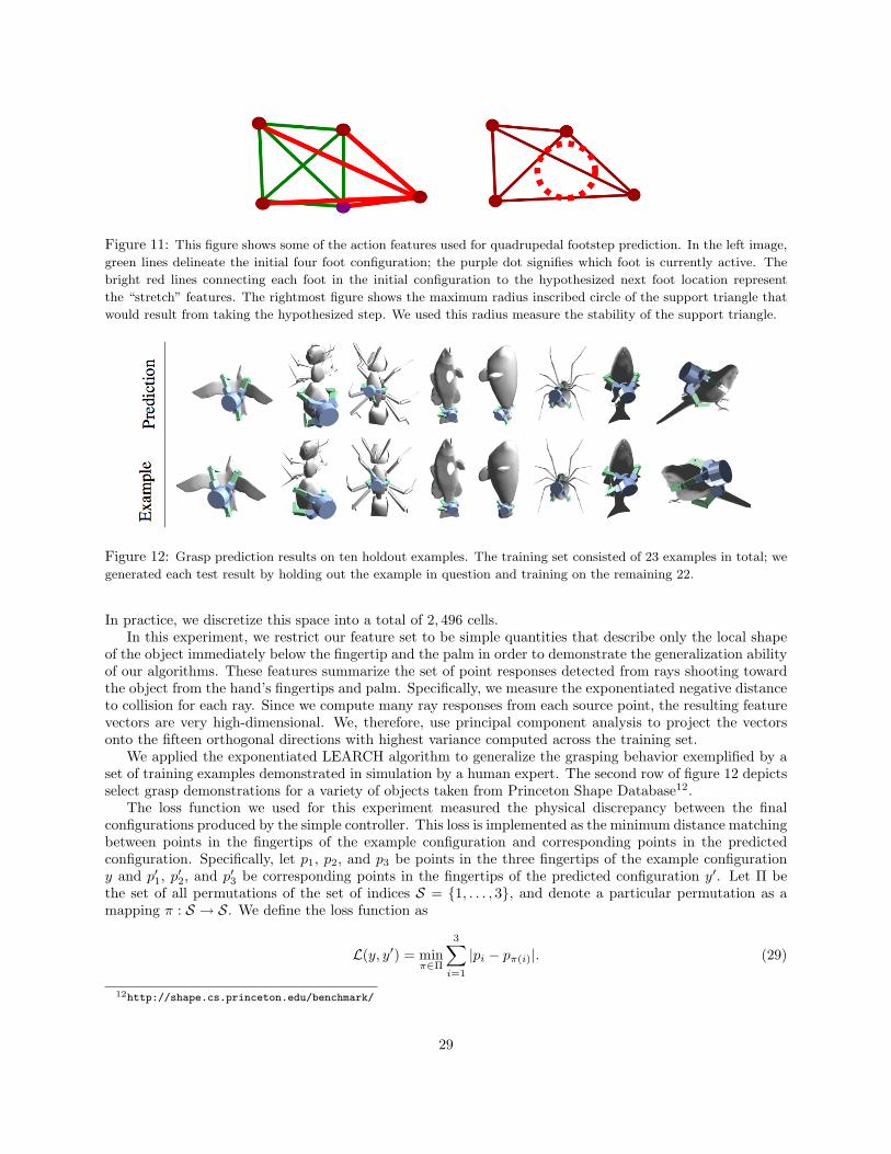
Figure 11: This figure shows some of the action features used for quadrupedal footstep prediction. In the left image,

green lines delineate the initial four foot configuration; the purple dot signifies which foot is currently active. The

bright red lines connecting each foot in the initial configuration to the hypothesized next foot location represent

the “stretch” features. The rightmost figure shows the maximum radius inscribed circle of the support triangle that

would result from taking the hypothesized step. We used this radius measure the stability of the support triangle.

Figure 12: Grasp prediction results on ten holdout examples. The training set consisted of 23 examples in total; we

generated each test result by holding out the example in question and training on the remaining 22.

In practice, we discretize this space into a total of 2, 496 cells.In this experiment, we restrict our feature set to be simple quantities that describe only the local shape

of the object immediately below the fingertip and the palm in order to demonstrate the generalization abilityof our algorithms. These features summarize the set of point responses detected from rays shooting towardthe object from the hand’s fingertips and palm. Specifically, we measure the exponentiated negative distanceto collision for each ray. Since we compute many ray responses from each source point, the resulting featurevectors are very high-dimensional. We, therefore, use principal component analysis to project the vectorsonto the fifteen orthogonal directions with highest variance computed across the training set.

We applied the exponentiated LEARCH algorithm to generalize the grasping behavior exemplified by aset of training examples demonstrated in simulation by a human expert. The second row of figure 12 depictsselect grasp demonstrations for a variety of objects taken from Princeton Shape Database12.

The loss function we used for this experiment measured the physical discrepancy between the finalconfigurations produced by the simple controller. This loss is implemented as the minimum distance matchingbetween points in the fingertips of the example configuration and corresponding points in the predictedconfiguration. Specifically, let p1, p2, and p3 be points in the three fingertips of the example configurationy and p′1, p′2, and p′3 be corresponding points in the fingertips of the predicted configuration y′. Let Π bethe set of all permutations of the set of indices S = {1, . . . , 3}, and denote a particular permutation as amapping π : S → S. We define the loss function as

L(y, y′) = minπ∈Π

3∑i=1

|pi − pπ(i)|. (29)

12http://shape.cs.princeton.edu/benchmark/

29

Figure 13: The first three images from the left demonstrate grasp generalization from multiple approach direction

on a single object. The final two images show from two perspectives a unique grasp that arises because of the simple

feature set. See the text for details.

Figure 14: The path traveled during two runs of an autonomous robot moving from top-left to bottom-right.The green run had no prior map, and made several poor decisions that required backtracking. The red runhad the prior costmap shown at right, and took a more efficient route. Brighter pixels indicate higher cost.

This gives low loss to configurations that are similar despite having vastly differing grasp parameters dueto symmetries in the hand, while still giving high loss to configurations that are physically different. Im-portantly, since the cost function is defined as a function of local shape descriptive features, configurationswith different grasp parameters but low loss under this loss function will tend to have similar features andtherefore similar costs. This property allows functionally similar grasps to be assigned similar costs duringlearning without being artificially penalized for being different from the desired grasp parameters in termsof Euclidean distance through the parameter space.

Figure 12 shows our test predictions (from a holdout set) side-by-side with the grasp the human wouldhave predicted for the problem. The algorithm typically generalizes well. It often learns concepts reminiscentof form closure for these unseen objects.

6 Case study: Structured imitation learning for outdoor naviga-tion from overhead data

In this section, we demonstrate the application of the LEARCH algorithm to the interpretation of overheaddata sources for use in long range navigation. This work is covered in detail in (Silver et al., 2008).

6.1 Outdoor navigation from overhead data

This work was performed in the context of the DARPA UPI program. UPI utilizes a six wheeled, skid steervehicle capable of traversing extreme terrains (Figure 1). With Crusher, UPI has pursued research intolong range navigation through complex, unstructured environments. Crusher is equipped with laser rangefinders and cameras for on-board perception. A perception system processes this sensory data to producetraversability costs that are merged with any prior cost data into a single map. Due to the dynamic nature of

30

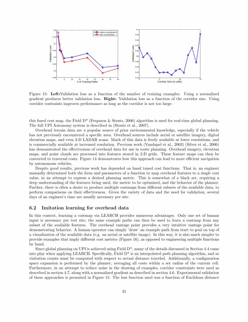
0 5 10 15 20 25 30 35 400.45

0.5

0.55

0.6

0.65

0.7

0.75

0.8

# of Training Paths

Val

idat

ion

Loss

without normalizationwith normalization

0 5 10 150.42

0.44

0.46

0.48

0.5

0.52

0.54

0.56

0.58

0.6

Corridor Size (in cells)

Val

idat

ion

Loss

Figure 15: Left:Validation loss as a function of the number of training examples. Using a normalizedgradient produces better validation loss. Right: Validation loss as a function of the corridor size. Usingcorridor contraints improves performance as long as the corridor is not too large.

this fused cost map, the Field D* (Ferguson & Stentz, 2006) algorithm is used for real-time global planning.The full UPI Autonomy system is described in (Stentz et al., 2007).

Overhead terrain data are a popular source of prior environmental knowledge, especially if the vehiclehas not previously encountered a specific area. Overhead sources include aerial or satellite imagery, digitalelevation maps, and even 3-D LADAR scans. Much of this data is freely available at lower resolutions, andis commercially available at increased resolution. Previous work (Vandapel et al., 2003) (Silver et al., 2006)has demonstrated the effectiveness of overhead data for use in route planning. Overhead imagery, elevationmaps, and point clouds are processed into features stored in 2-D grids. These feature maps can then beconverted to traversal costs. Figure 14 demonstrates how this approach can lead to more efficient navigationby autonomous vehicles.

Despite good results, previous work has depended on hand tuned cost functions. That is, an engineermanually determined both the form and parameters of a function to map overhead features to a single costvalue, in an attempt to express a desired planning metric. This is somewhat of a black art, requiring adeep understanding of the features being used, the metric to be optimized, and the behavior of the planner.Further, there is often a desire to produce multiple costmaps from different subsets of the available data, toperform comparisons on their effectiveness. Given the variety of data and the need for validation, severaldays of an engineer’s time are usually necessary per site.

6.2 Imitation learning for overhead data

In this context, learning a costmap via LEARCH provides numerous advantages. Only one set of humaninput is necessary per test site; the same example paths can then be used to learn a costmap from anysubset of the available features. The overhead vantage point provides a very intuitive vantage point fordemonstrating behavior. A human operator can simply ’draw’ an example path from start to goal on top ofa visualization of the available data (e.g. an aerial or satellite image). In this way, it is also much simpler toprovide examples that imply different cost metrics (Figure 16), as opposed to engineering multiple functionsby hand.

Since global planning on UPI is achieved using Field D*, many of the details discussed in Section 4.4 cameinto play when applying LEARCH. Specifically, Field D* is an interpolated path planning algorithm, and sovisitation counts must be computed with respect to actual distance traveled. Additionally, a configurationspace expansion is performed by the planner, averaging all costs within a set radius of the current cell.Furthermore, in an attempt to reduce noise in the drawing of examples, corridor constraints were used asdescribed in section 4.7, along with a normalized gradient as described in section 4.6. Experimental validationof these approaches is presented in Figure 15. The loss function used was a function of Euclidean distance

31

Figure 16: Top: Example paths that imply different metrics (From top to bottom: minimize distancetraveled, stay on roads, stay near trees) Bottom: Learned costmaps from the corresponding examples(brighter pixels indicate higher cost). Imagery from the Quickbird satellite courtesy of Digital Globe, Inc.

between states on the current path µ and the closest state on the example µi, with a scale parameter σ2

L(µ, µi) =1|µ|∑s∈µ

1− exp ( minsi∈µi

[‖s− si‖2]/σ2)

LEARCH, as listed in Algorithm 5, was implemented with 4 varieties of regressors: linear, neural net-works, regression trees, and linear with a feature learning phase using regression trees (see section 4.5).Overall, the latter approach was found to provide superior all around performance. Specifically, the compu-tational advantage of log-linear LEARCH is quite desirable when rapid training was required. Additionally,using non-linear regressors often resulted in overfitting; performance was better on the training set but worseon a validation set. In contrast a linear cost function with a handful of simple regression trees provided goodperformance on both training and validation sets. It is interesting to note that at the conceptual levelthis approach is similar to the types of cost functions that were often generated by human engineering: agenerally linear cost function, with a few special cases handled differently.

6.3 Experimental results

Numerous offline experiments were performed to compare performance of different varieties of LEARCHapplied to overhead data, and to compare its performance to the hand-tuned approach. One experiment ofnote compared the generalization of LEARCH with that of a hand-tuned costmap. A cost map was trainedoff satellite imagery for an approximately 60 km2 size area at 60 cm resolution. An engineered costmap hadbeen previously produced for this same area to support UPI. A subset of both maps is shown in Figure 17.The two maps were compared using a validation set of paths generated by a UPI team member not directlyinvolved in the development of overhead costing. The average validation loss was 0.675 with the engineeredmap, and 0.551 with the LEARCH map.

Additional validation was also achieved during official UPI field tests. UPI field tests consist of Crusherautonomously navigating a series of courses, with each course defined as a set of widely spaced waypoints.Courses ranged in length up to 20 km, with waypoint spacing on the order of 200 to 1000 m. These tests tookplace at numerous locations across the continental U.S., each with highly varying local terrain characteristics,

32

Figure 17: A 10 km2 section of a UPI test site. From left to right: satellite imagery, LEARCH Cost, andEngineered Cost. Costmaps are Jet-Colored to highlight differences.Prominent features include roads, trails,grass, bushes, trees, and washes.

and sizes ranging from tens to hundreds of square kilometers.During 2005 and 2006, prior maps were primarily generated as described in (Silver et al., 2006). Satellite

Imagery and aerial fixed wing LADAR scans were used as input to multiple feature extractors and classifiers.These features were then fed into a hand tuned cost function. An initial implementation of the MMPalgorithm was also field tested and demonstrated in smaller tests during 2006. During 2007 and 2008,LEARCH became the default approach for producing cost maps. Overall, LEARCH maps were used duringmore than 600 km of sponsor monitored autonomous traverse, plus hundreds of kilometers more of additionalfield testing.

In addition, two direct online comparisons were performed. These two tests were performed severalmonths apart, at different test sites. During these experiments, the same course was run multiple times,varying only the overhead cost map given to Crusher. To score each run, cost according to Crusher’s highlyaccurate onboard perception system was used as an estimate of the ground truth risk incurred. Crusher’sperception system has been engineered13 over a period of years to enable safe autonomous navigation (evenwithout any overhead data), and makes use of data that is far higher resolution than overhead data. Theresults of these experiments are shown in Table 1. In both experiments, Crusher traveled farther to completethe same course using LEARCH produced cost maps, and yet was scored with less total cost by Crusher’sperception system. Crusher also was able to drive faster on average, an indication of more favorable ter-rain. The course for Experiment 2 was also run without any overhead data; the results are presented forcomparison.

7 Future directions

LEARCH is applicable to a wide range of problems in robotics. Our experiments demonstrate that whenapplicable, the algorithms enjoy fast training and strong generalization. However, its application to anygiven problem requires the existence of efficient MDP solvers. While efficient planning algorithms oftenform the backbone of modern robotics systems, as the dimensionality of the configuration space increases,these planners necessarily become approximations and are often stochastic. One of our current directions

13Crusher’s perception system provides an ideal scenario for dynamic imitation learning as mentioned in Section 7

33

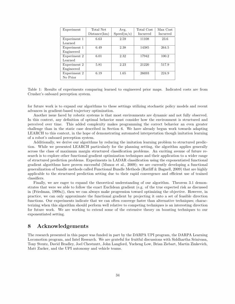
Experiment Total Net Avg. Total Cost Max CostDistance(km) Speed(m/s) Incurred Incurred

Experiment 1 6.63 2.59 11108 23.6Learned

Experiment 1 6.49 2.38 14385 264.5Engineered

Experiment 2 6.01 2.32 17942 100.2Learned

Experiment 2 5.81 2.23 21220 517.9Engineered

Experiment 2 6.19 1.65 26693 224.9No Prior

Table 1: Results of experiments comparing learned to engineered prior maps. Indicated costs are fromCrusher’s onboard perception system.

for future work is to expand our algorithms to these settings utilizing stochastic policy models and recentadvances in gradient-based trajectory optimization.

Another issue faced by robotic systems is that most environments are dynamic and not fully observed.In this context, any definition of optimal behavior must consider how the environment is structured andperceived over time. This added complexity makes programming the correct behavior an even greaterchallenge than in the static case described in Section 6. We have already begun work towards adaptingLEARCH to this context, in the hope of demonstrating automated interpretation though imitation learningof a robot’s onboard perception system.

Additionally, we derive our algorithms by reducing the imitation learning problem to structured predic-tion. While we presented LEARCH particularly for the planning setting, the algorithm applies generallyacross the class of maximum margin structured classification problems. An exciting avenue of future re-search is to explore other functional gradient optimization techniques and their application to a wider rangeof structured prediction problems. Experiments in LADAR classification using the exponentiated functionalgradient algorithms have proven successful (Munoz et al., 2009); we are currently developing a functionalgeneralization of bundle methods called Functional Bundle Methods (Ratliff & Bagnell, 2009) that are highlyapplicable to the structured prediction setting due to their rapid convergence and efficient use of trainedclassifiers.

Finally, we are eager to expand the theoretical understanding of our algorithm. Theorem 3.1 demon-strates that were we able to follow the exact Euclidean gradient (e.g. of the true expected risk as discussedin (Friedman, 1999a)), then we can always make progression toward optimizing the objective. However, inpractice, we can only approximate the functional gradient by projecting it onto a set of feasible directionfunctions. Our experiments indicate that we can often converge faster than alternative techniques; charac-terizing when this algorithm should perform well relative to competing techniques is an interesting directionfor future work. We are working to extend some of the extensive theory on boosting techniques to ourexponentiated setting.

8 Acknowledgements

The research presented in this paper was funded in part by the DARPA UPI program, the DARPA LearningLocomotion program, and Intel Research. We are grateful for fruitful discussions with Siddhartha Srinivasa,Tony Stentz, David Bradley, Joel Chestnutt, John Langford, Yucheng Low, Brian Ziebart, Martin Zinkevich,Matt Zucker, and the UPI autonomy and vehicle teams.

34

References

Abbeel, P., & Ng, A. Y. (2004). Apprenticeship learning via inverse reinforcement learning. ICML ’04: Proceedingsof the twenty-first international conference on Machine learning.

Anderson, B. D. O., & Moore, J. B. (1990). Optimal control: linear quadratic methods. Prentice Hall, EnglewoodCliffs, N.J.

Argall, B., Chernova, S., Veloso, M., & Browning, B. (2009). A survey of robot learning from demonstration. Roboticsand Autonomous Systems.

Atkeson, C., Schaal, S., & Moore, A. (1995). Locally weighted learning. AI Review.

Bain, M., & Sammut, C. (1995). A framework for behavioral cloning. Machine Intelligence Agents. Oxford UniversityPress.

Boyd, S., Ghaoui, L. E., Feron, E., & Balakrishnan, V. (1994). Linear matrix inequalities in system and controltheory. Society for Industrial and Applied Mathematics (SIAM).

Calinon, S., Guenter, F., & Billard, A. (2007). On learning, representing and generalizing a task in a humanoidrobot. IEEE transactions on systems, man and cybernetics, Part B. Special issue on robot learning by observation,demonstration and imitation, 37, 286–298.

Cesa-Bianchi, N., & Lugosi, G. (2006). Prediction, learning, and games. New York, NY, USA: Cambridge UniversityPress.

Chestnutt, J., Kuffner, J., Nishiwaki, K., & Kagami, S. (2003). Planning biped navigation strategies in complexenvironments. Proceedings of the IEEE-RAS International Conference on Humanoid Robots. Karlsruhe, Germany.

Chestnutt, J., Lau, M., Cheng, G., Kuffner, J., Hodgins, J., & Kanade, T. (2005). Footstep planning for the HondaASIMO humanoid. Proceedings of the IEEE International Conference on Robotics and Automation.

Donoho, D. L., & Elad, M. (2003). Maximal sparsity representation via l1 minimization. the Proc. Nat. Aca. Sci.100 (pp. 2197–2202).

Ferguson, D., & Stentz, A. (2006). Using interpolation to improve path planning: The field D* algorithm. Journalof Field Robotics, 23, 79–101.

Friedman, J. H. (1999a). Greedy function approximation: A gradient boosting machine. Annals of Statistics.

Gordon, G. (1999). Approximate solutions to markov decision processes. Doctoral dissertation, Robotics Institute,Carnegie Mellon University.

Hersch, M., Guenter, F., Calinon, S., & Billard, A. (2008). Dynamical system modulation for robot learning viakinesthetic demonstrations. IEEE Transactions on Robotics, 24, 1463–1467.

Jaynes, E. (2003). Probability: The logic of science. Cambridge University Press.

Kalman, R. (1964). When is a linear control system optimal? Trans. ASME, J. Basic Engrg., 86, 51–60.

Kelly, A., Amidi, O., Happold, M., Herman, H., Pilarski, T., Rander, P., Stentz, A., Vallidis, N., & Warner, R.(2004). Toward reliable autonomous vehicles operating in challenging environments. Proceedings of the InternationalSymposium on Experimental Robotics (ISER). Singapore.

Kivinen, J., & Warmuth, M. K. (1997). Exponentiated gradient versus gradient descent for linear predictors. Infor-mation and Computation, 132.

Kolter, J. Z., Abbeel, P., & Ng, A. Y. (2008). Hierarchical apprenticeship learning with application to quadrupedlocomotion. Neural Information Processing Systems 20.

Kulesza, A., & Pereira, F. (2008). Structured learning with approximate inference. Advances in Neural InformationProcessing Systems. MIT Press.

LeCun, Y., Muller, U., Ben, J., Cosatto, E., & Flepp, B. (2006). Off-road obstacle avoidance through end-to-endlearning. Advances in Neural Information Processing Systems 18. MIT Press.

Mason, L., J.Baxter, Bartlett, P., & Frean, M. (1999). Functional gradient techniques for combining hypotheses.Advances in Large Margin Classifiers. MIT Press.

Miller, A. T., Knoop, S., Allen, P. K., & Christensen, H. I. (2003). Automatic grasp planning using shape primitives.Proceedings of the IEEE International Conference on Robotics and Automation.

35

Munoz, D., Bagnell, J. A. D., Vandapel, N., & Hebert, M. (2009). Contextual classification with functional max-margin markov networks. IEEE Computer Society Conference on Computer Vision and Pattern Recognition(CVPR).

Munoz, D., Vandapel, N., & Hebert, M. (2008). Directional associative markov network for 3-d point cloud classifi-cation. Fourth International Symposium on 3D Data Processing, Visualization and Transmission.

Neu, G., & Szepesvari, C. (2007). Apprenticeship learning using inverse reinforcement learning and gradient methods.Uncertainty in Artificial Intelligence (UAI).

Ng, A. Y., & Russell, S. (2000). Algorithms for inverse reinforcement learning. Proc. 17th International Conf. onMachine Learning.

Pomerleau, D. (1989). ALVINN: An Autonomous Land Vehicle in a Neural Network. Advances in Neural InformationProcessing Systems 1.

Puterman, M. (1994). Markov decision processes: Discrete stochastic dynamic programming. Wiley.

Ratliff, N., & Bagnell, J. A. (2009). Functional bundle methods. The Learning Workshop. Clearwater Beach, Forida.

Ratliff, N., Bagnell, J. A., & Zinkevich, M. (2006a). Maximum margin planning. Twenty Second InternationalConference on Machine Learning (ICML06).

Ratliff, N., Bagnell, J. A., & Zinkevich, M. (2007a). (Online) subgradient methods for structured prediction. ArtificialIntelligence and Statistics. San Juan, Puerto Rico.

Ratliff, N., Bradley, D., Bagnell, J. A., & Chestnutt, J. (2006b). Boosting structured prediction for imitation learning.NIPS. Vancouver, B.C.

Ratliff, N., Srinivasa, S., & Bagnell, J. A. (2007b). Imitation learning for locomotion and manipulation. IEEE-RASInternational Conference on Humanoid Robots.

Rifkin, Y., & Poggio (2003). Regularized least squares classification. Advances in Learning Theory: Methods, Modelsand Applications. IOS Press.

Rosset, S., Zhu, J., & Hastie, T. (2004). Boosting as a regularized path to a maximum margin classifier. J. Mach.Learn. Res., 5, 941–973.

Schaal, S., & Atkeson, C. (1994). Robot juggling: An implementation of memory-based learning. IEEE ControlSystems Magazine, 14.

Shor, N. Z. (1985). Minimization methods for non-differentiable functions. Springer-Verlag.

Silver, D., Bagnell, J. A., & Stentz, A. (2008). High performance outdoor navigation from overhead data usingimitation learning. Proceedings of Robotics Science and Systems.

Silver, D., Sofman, B., Vandapel, N., Bagnell, J. A., & Stentz, A. (2006). Experimental analysis of overhead dataprocessing to support long range navigation. Proceedings of the IEEE/JRS International Conference on IntelligentRobots and Systems.

Stentz, A., Bares, J., Pilarski, T., & Stager, D. (2007). The crusher system for autonomous navigation. AUVSIsUnmanned Systems.

Taskar, B., Chatalbashev, V., Guestrin, C., & Koller, D. (2005). Learning structured prediction models: A largemargin approach. Twenty Second International Conference on Machine Learning (ICML05).

Taskar, B., Guestrin, C., & Koller, D. (2003). Max margin markov networks. Advances in Neural InformationProcessing Systems (NIPS-14).

Taskar, B., Lacoste-Julien, S., & Jordan, M. (2006). Structured prediction via the extragradient method. In Advancesin neural information processing systems 18. MIT Press.

Tropp, J. A. (2004). Greed is good: Algorithmic results for sparse approximation. IEEE Trans. Inform. Theory, 50,2231–2242.

Vandapel, N., Donamukkala, R. R., & Hebert, M. (2003). Quality assessment of traversability maps from aeriallidar data for an unmanned ground vehicle. Proceedings of the IEEE/JRS International Conference on IntelligentRobots and Systems.

Ziebart, B., Bagnell, J. A., Mass, A., & Dey, A. (2008). Maximum entropy inverse reinforcement learning. Twenty-third AAAI Conference.

Zinkevich, M. (2003). Online convex programming and generalized infinitesimal gradient ascent. Proceedings of theTwentieth International Conference on Machine Learning.

36