Embed Size (px)
Citation preview
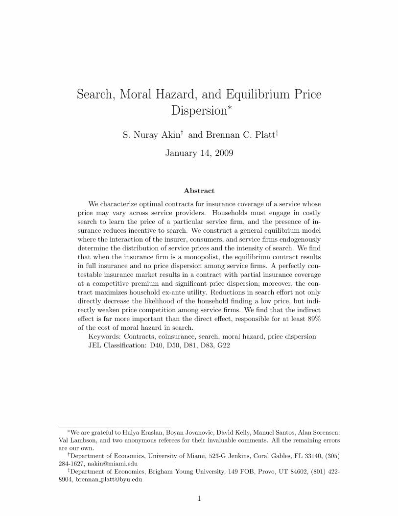
Search, Moral Hazard, and Equilibrium PriceDispersion∗
S. Nuray Akin† and Brennan C. Platt‡
January 14, 2009
Abstract
We characterize optimal contracts for insurance coverage of a service whoseprice may vary across service providers. Households must engage in costlysearch to learn the price of a particular service firm, and the presence of in-surance reduces incentive to search. We construct a general equilibrium modelwhere the interaction of the insurer, consumers, and service firms endogenouslydetermine the distribution of service prices and the intensity of search. We findthat when the insurance firm is a monopolist, the equilibrium contract resultsin full insurance and no price dispersion among service firms. A perfectly con-testable insurance market results in a contract with partial insurance coverageat a competitive premium and significant price dispersion; moreover, the con-tract maximizes household ex-ante utility. Reductions in search effort not onlydirectly decrease the likelihood of the household finding a low price, but indi-rectly weaken price competition among service firms. We find that the indirecteffect is far more important than the direct effect, responsible for at least 89%of the cost of moral hazard in search.
Keywords: Contracts, coinsurance, search, moral hazard, price dispersionJEL Classification: D40, D50, D81, D83, G22
∗We are grateful to Hulya Eraslan, Boyan Jovanovic, David Kelly, Manuel Santos, Alan Sorensen,Val Lambson, and two anonymous referees for their invaluable comments. All the remaining errorsare our own.†Department of Economics, University of Miami, 523-G Jenkins, Coral Gables, FL 33140, (305)
284-1627, [email protected]‡Department of Economics, Brigham Young University, 149 FOB, Provo, UT 84602, (801) 422-
8904, brennan [email protected]
1

1 Introduction
In most markets where insurance plays a prominent role (such as medical services or
auto repairs), the price of a particular service varies significantly from one firm to
another.1 In a typical market, consumers respond to price dispersion by obtaining
price quotes from a number of firms and selecting the lowest price. However, when an
insurance company ultimately pays for most of the service, the consumer’s incentive
to search is dramatically reduced — most of the price reduction obtained through
search effort is passed on to the insurance company. With fewer searches, sales prices
(and thus the expected insurance payout) are higher. This paper studies the optimal
insurance contract in an environment with moral hazard due to search.
An insurance contract (or policy) consists of the premium charged to households
as well as a coinsurance rate, defined as the percentage of an insurance claim that
the household pays out-of-pocket. In offering a particular policy, an insurer must
consider the incentives it creates for both households and service-providing firms. We
depict this in a general equilibrium model in which the interactions between these
agents endogenously determine the insurance policy, the distribution of service prices,
and the search intensity of households. We find that when the insurance firm is a
monopolist, the equilibrium contract results in full insurance and no price dispersion
among service firms. However, when the insurance market is perfectly contestable,
the threat of competition results in a contract with a competitive premium and only
partial insurance coverage. More interestingly, this contract is also the one that
maximizes household expected utility.
Furthermore, we examine the magnitude of moral hazard in search, measured as
the change in the expected total cost2 of the event due to the presence of insurance.
We decompose two effects which contribute to this rise in expected cost. First, a
direct effect occurs when consumers request fewer quotes from the same distribution.
Second, an indirect effect occurs because requesting fewer quotes results in less price
competition among the firms, shifting the distribution toward higher prices. Indeed,
we find that the latter effect is at least 8.6 times bigger than the former (for all
1Sorensen (2000) provides an empirical investigation of price dispersion in the prescription drugmarket (pricing the same drug across retailers). He documents that, on average, the highest postedprice is over 50 percent above the lowest available price; furthermore, differences in pharmacy char-acteristics can account for at most 1/3 of the dispersion.
2This is defined as the insurance premium plus expected out-of-pocket and search costs.
2

parameter values), or in other words, is responsible for at least 89% of the total cost
of moral hazard. Thus, the general equilibrium feedback is in fact the much larger
concern in the incentive problem. To our knowledge, we are the first to distinguish
this effect within the optimal contract literature.
In our model, there is a continuum of ex-ante identical households and service
firms, and an insurance firm. Households face a random event (such as an auto
accident or health problem) with some fixed probability. If the event occurs, the
household hires a service firm to fully repair the damage.3 This service is homogenous
across the service firms, but each firm may charge a different price. Households know
the distribution of offered prices, but can only learn the price charged by a particular
firm by requesting a quote at a constant cost.
Households can insure against this event by purchasing a policy offered by the
insurance firm, which specifies a premium as well as a coinsurance rate. If the event
occurs, the policy reimburses a fraction of the actual price paid. We initially analyze
household and service firm choices while taking the insurance contract as given. We
then augment the model by endogenizing the choice of contract offered by the insur-
ance firm, which anticipates the subgame equilibrium behavior from the preceeding
analysis.
We consider the insurance firm under two different market structures. In the first,
they act as a pure monopolist. In the second, they are the only insurer but the
market is perfectly contestable; that is, there are no barriers to entry or sunk costs.4
All service firms are within the insurer’s approved network, meaning they have agreed
not to charge more than an exogenously-set maximum allowable price.
In the endogenous contract model, decisions occur in the following order: First,
the insurance firm chooses which policy to offer. Households then accept or reject
this policy. Next, service firms simultaneously set their prices. Finally, the event is
realized for some of the households, who then must decide how many quotes to re-
quest and select the lowest price among them. Search is simultaneous, as in Burdett
and Judd (1983); that is, a household receives all quotes at the same time. Unlike
sequential search, a simultaneous search environment can generate equilibrium price
3This is purely a monetary loss, then, and ignores any irreparable damage. Ma and McGuire(1997) also model health shocks as a monetary loss which can be partially recovered depending onthe quantity and quality of health care purchased.
4We do not consider the case in which several contracts are offered (by one or by many firms),as this becomes analytically intractable.
3

dispersion even though firms and households are homogeneous. Also, this environ-
ment approximates a situation in which the repair or surgery must take place within a
short timeframe; Manning and Morgan (1982) and Morgan and Manning (1985) offer
this and several other scenarios in which simultaneous search dominates sequential
search.
Our model abstracts from some of the institutional details of insurance. For
instance, all firms are assumed to be in the insurer’s preferred provider network; that
is, households never consider firms outside of their network. Since out-of-network
prices are typically higher and their insurance reimbursement is less generous, this
is probably an accurate depiction of most household choices. The exceptions are
when emergency service is needed while traveling outside of the network area, or
when significant quality differences exist among firms — both of which are beyond
the scope of this model. Also, we do not model the negotiation process by which
the maximum allowable price is set, nor can insurers engage in search on behalf of
households.
Whenever the presence of insurance distorts incentives for the insured, causing
an increase in expected payout, a moral hazard problem occurs. Two other forms of
moral hazard are well known. First, the insured person may exercise less precaution
(such as defensive driving), increasing the probability of loss. Second, the insured
person may increase his consumption of the covered service (such as medical appoint-
ments), increasing the size of loss. These have been extensively studied, beginning
with the work of Arrow (1963), Pauly (1968), Smith (1968), Zeuckhauser (1970), and
Ehrlich and Becker (1972).
However, moral hazard in search has received much less attention, with the only
formal analyses in Dionne (1981, 1984).5 In a model where the coinsurance rate is
taken as exogenous and the distribution of prices is fixed regardless of the number
of quotes requested by households, Dionne identifies the negative incentive effect of
insurance on search behavior and hence on expected service prices. However, he
neglects a crucial (and, as we show, larger) component of the story: the endogenous
response of firms to household search.
There is substantial evidence of a positive relationship between insurance coverage
5Arrow (1963) mentions the potential problem: “Insurance removes the incentive on the part ofindividuals, patients, and physicians to shop around for better prices for hospitalization and surgicalcare.”
4

and service firm prices. Using a product-level panel dataset of various drug purchases
in Germany, Pavcnik (2002) shows that prices decreased significantly after a change
in insurance coverage that made households responsible for a larger portion of their
prescription purchases. Feldstein (1970, 1971) find that physicians and non-profit
hospitals raise their prices as insurance coverage becomes more extensive. In fact,
Feldstein (1973) estimates that raising the coinsurance rate for hospital stays from
33 to 50 percent would reduce prices sufficiently to increase welfare between 11 and
25 percent (net of the welfare cost of increased exposure to risk).
This paper relates to the optimal insurance literature, such as Crew (1969), Smith
(1968), Pauly (1968), and Gaynor, Haas-Wilson, and Vogt (2000). In particular, Ma
and McGuire (1997) shares the same spirit as our paper, though they examine a differ-
ent aspect of moral hazard. In their model, health insurance contracts are incomplete
because the quantity and quality of health care is not contractible; household or
physician effort are hidden to some degree. This is a variation of moral hazard in
consumption — households use more services, and physicians provide lower quality
care. Our model follows a similar timing of insurance, service firm, and household
decisions; but instead, the non-contractible elements are firm pricing and household
quote requests, leading to moral hazard in search.
Nell, Richter, and Schiller (2008) also model the interaction between coinsurance
and service prices. In their environment, product differentiation among service firms
gives them spatial market power; thus, even though households are perfectly informed,
they may choose to fill their prescription from a more expensive pharmacy, for in-
stance. In this sense, moral hazard arises because insurance is non-contractible on
the location of purchase. However, there is no price dispersion in their analysis: they
concentrate on symmetric equilibrium where all firms charge the same price.
The paper proceeds as follows: Section 2 presents the model in which the insurance
contract is exogenous, and characterizes the equilibrium behavior of service firms
and households. Insurance contracts are endogenized in Section 3, and the optimal
contract is characterized. Section 4 applies the model to prescription drug insurance,
developing a numerical example which illustrates equilibrium behavior. Section 5
provides a measure of moral hazard in search and decomposes this into the direct and
indirect effect. Finally, we offer conclusions in Section 6.
5

2 Exogenous Insurance Contract
2.1 Environment
Three types of agents interact in this economy: households, service firms, and an
insurance firm. We assume a continuum (of measure one) of both households and
service firms. Within each type, agents are identical ex-ante.
Households face a random event (such as an auto accident or health problem)
with probability ρ. When the event occurs, the household hires a service firm to fully
repair the damage. This service is homogenous across the service firms, but each
firm may charge a different price. Households know the distribution of offered prices,
F (p), but can only learn the price p charged by a particular firm by requesting a
quote at a cost c > 0.
Households insure against this event by purchasing a policy offered by the insur-
ance firm, which specifies a premium θ as well as a coinsurance rate γ. We initially
consider this insurance contract as exogenously given and assume that all households
insure; in Section 3, both the insurance policy and the decision to purchase it are
endogenously determined. If the event occurs, the policy reimburses a fraction 1− γof the actual price paid. All service firms are within the insurer’s approved network,
meaning they have agreed not to charge more than an exogenously-set maximum
allowable price M .
Note that demand for the service is perfectly inelastic; fraction ρ of the population
will always purchase one unit of service from some firm. The only question is what
price they will pay for it. This assumed demand is needed to isolate the effect of
moral hazard in search. If consumers had any elasticity in their demand, then the
presence of insurance would encourage them to consume more units of service, which
is moral hazard in consumption.
Decisions occur in the following order: Service firms simultaneously set their
prices. Then the event is realized for some of the households, who must decide how
many quotes to request and select the lowest price among them.
2.2 Household Quote Requests
In the last stage of the game, only those unlucky households who experience the
event have a choice to make: the number n of quotes to request. At that point, the
6

distribution of service prices is fixed. The quotes are all received simultaneously, after
which the household will choose the lowest among them.6
Household utility, u(w), is a Bernoulli utility function for money. To create a role
for insurance, we assume that households are risk averse — in particular, u′ > 0 and
u′′ < 0 for all w. The choice of n is made so as to maximize expected utility:
EU(θ, γ, F (·)) ≡ maxn∈Z
∫ M
¯p
u (w − θ − cn− γp)n(1− F (p))n−1dF (p). (1)
The analysis of this model is far more tractable if the objective function in Equa-
tion 1 is a strictly concave function of n. Since n is restricted to integer values,
strict concavity ensures that there will either be a unique solution n∗ or households
will be indifferent between requesting either n∗ or n∗ + 1 quotes. If u(·) were linear
utility, concavity would be a simple property of order statistics; obtaining the same
with risk averse households requires further restrictions on utility (which are imposed
throughout the paper).7
Proposition 1. Given increasing and concave u(·) with decreasing absolute risk aver-
sion, expected utility is strictly concave with respect to n.
Proof. First, expected utility can be transformed via integration by parts to become:
u(w − θ − cn− γ¯p)− γ
∫ M
¯p
u′(w − θ − cn− γp)(1− F (p))ndp.
The second derivative (w.r.t. n) of this expression of expected utility is:
c2u′′(w − θ − cn− γ¯p)−
γ
∫ M
¯p
(1− F (p))n([ln(1− F (p))]2 u′(·)− 2c ln(1− F (p))u′′(·) + c2u′′′(·)
)dp.
Since absolute risk aversion is measured by a(w) = −u′′(w)u′(w)
, then decreasing ab-
solute risk aversion, a′(w) < 0, implies (u′′)2 < u′u′′′. Since u′ > 0, u′′′ > 0 as well.
6There is no option to seek another set of quotes, even if the first set were clustered on the highend of the distribution. Also, requesting a quote is prerequisite to obtaining service, so all unluckyhouseholds must have n ≥ 1.
7These assumptions are sufficient but not necessary to obtain concavity with respect to n; how-ever, it is difficult to find less restrictive yet intuitive assumptions on u(·) or F (·) that ensure theresult.
7

Because u′′ < 0, we have |u′′| <√u′u′′′ =⇒ u′′ > −
√u′u′′′ for any w.
Note that ln(1− F (p)) < 0. Thus, for all p,
(1− F (p))n([ln(1− F (p))]2 u′(·)− 2c ln(1− F (p))u′′(·) + c2u′′′(·)
)> (1− F (p))n
([ln(1− F (p))]2 u′(·) + 2c ln(1− F (p))
√u′(·)u′′′(·) + c2u′′′(·)
)= (1− F (p))n
(ln(1− F (p))
√u′(·) + c
√u′′′(·)
)2
> 0.
Hence, in the expression of the second derivative, the integrand is always a positive
number, making the second term negative. The first term is also negative because
u′′ < 0.
Thus, it is possible for ex-ante identical households to choose different numbers of
quote requests, but with the concavity of EU , this only occurs over two consecutive
numbers and the households must be indifferent between them. Among all households
who incur losses, the fraction who request n quotes is expressed as qn.
2.3 Service Firms
The individual service firms are able to repair a household’s loss at constant marginal
cost r. We assume r < M . Each firm sets a price p, taking as given the distribution
of prices among other firms and the search behavior of consumers, represented by
F (·) and qn.8 Only ρ percent of the population will be in the market for their service,
and among those customers, a firm will only make the sale if its quoted price is lower
than all other quotes requested by that customer. Thus, a firm considers not only
the profit per sale, p − r, but also the probability of making the sale, as depicted in
the firm’s expected profit:
maxp
ΠS(p) ≡
ρ(p− r)∑∞
n=1 qnn(1− F (p))n−1 if p ≤M
0 if p > M.(2)
A Service Firm Equilibrium is a price distribution F (·) and service firm profit ΠS
such that, given the aggregate distribution of quote requests {qn}∞n=1,
8In particular, an individual firm does not expect that raising its price will result in fewer searches,since it is only one of the continuum of firms and cannot affect the price distribution. This wouldonly occur if a positive mass of firms raised their prices.
8

1. ΠS = ΠS(p) for all p in the support of F (·)
2. ΠS ≥ ΠS(p) for all p.
In a service firm equilibrium, each firm is indifferent among all prices in the support.
Thus, the price distribution may be interpreted in one of two ways. Each firm could
select a particular price in the support with certainty, with an aggregate distribution
F (·) of those prices. Alternatively, one could see F (·) as the mixed strategy employed
by every firm in a symmetric equilibrium.
For any particular insurance policy (θ, γ), the interaction of service firms and
households will determine the number of quote requests and the price distribution.
An Insured Search Equilibrium for (θ, γ) is a price distribution F (·), service firm
profits ΠS, and a distribution of household quote requests {qn}∞n=1 such that:
1. F (·) and ΠS constitute a service firm equilibrium given {qn}∞n=1
2. qn > 0 only if n solves the household’s problem (Eq. 1)
3.∑∞
n=1 qn = 1.
If the equilibrium F (·) is a non-degenerate distribution, we refer to it as a dispersed
price equilibrium.
2.4 Search and Price Dispersion
Before combining the interaction of household search and firm pricing, we note that
the behavior of service firms in this model replicates that of firms in Burdett and
Judd (1983). Thus all of their results (summarized in this subsection) concerning
firms directly apply. In particular:
• If q1 = 1, the unique service firm equilibrium has F (M) = 1 and F (p) = 0 for
p < M . In that case, ΠS = ρ(M − r). That is, if everyone requests a single
quote, there is no reason to compete on price, so everyone charges the maximum
allowed.
• If q1 = 0, the unique service firm equilibrium has F (r) = 1 and F (p) = 0 for
p < r. In that case, ΠS = 0. If everyone requests more than one quote, price
competition will drive all firms to charge marginal cost.
9

• If q1 ∈ (0, 1), the unique service firm equilibrium has continuous F (·), with
support [¯p,M ], for some
¯p > r. A dispersed price distribution can only arise
if some fraction of the population requests only one bid. If so, some firms will
offer high prices (including M), hoping to capture those who only ask for one
quote; others will offer lower prices in pursuit of those who request multiple
quotes.
By combining these results with household search behavior, we can further narrow
the possible insured search equilibria. For instance, no equilibrium exists in which
q1 = 0. In that case, a service firm equilibrium would require a degenerate price
distribution, concentrated at r. But if all firms choose the same price r, there would
be no reason for households to request more than one quote, requiring that q1 = 1.
On the other hand, an insured search equilibrium always exists in which q1 = 1
and all firms charge price M . These choices are mutually consistent, since no firm
will be undercut if no one searches twice, and no household should search multiple
times if all prices are identical. This sort of result is common to all search models.
Having eliminated the other possibility for a degenerate price distribution, we may
appropriately refer to this as the degenerate equilibrium.
In order to have a dispersed price equilibrium, we need 0 < q1 < 1. Because of
the concavity of the utility function with respect to n, this means that q2 = 1− q1; if
households were indifferent between 1 and n, then the quantities from 2 to n−1 would
all produce strictly more utility. For notational ease, we set q = q1. The existence
of such an equilibrium depends on the parameters. For instance, when the cost of
search is sufficiently high, no one can be enticed to search twice.
For a dispersed price equilibrium, the service firm’s profit can be written as:
ΠS(p) = ρ(p− r)(q+ 2(1− q)(1−F (p))). As stated earlier, F (p) must be continuous
when q ∈ (0, 1). We can determine the precise distribution associated with a given q
based on the requirement that all prices in the support be equally profitable. Thus
(M − r)q = (p− r)(q + 2(1− q)(1− F (p))), which yields:
F (p) = 1− (M − p)q2(p− r)(1− q)
for p ∈[¯p,M
]. (3)
The lower bound,¯p ≡ r + (M−r)q
2−q , is derived such that F (¯p) = 0. Also, dF (p) =
(M−r)q2(1−q)(p−r)2 . Each service firm has an ex-ante expected profit of ΠS = ρq(M − r).
Thus, firm behavior and the resulting price distribution are entirely determined by
10

q, the fraction of people who request only one quote. Furthermore, a larger q results
in prices more concentrated on the right tail of the distribution, as established in the
following lemma.
Lemma 1. If q′ < q′′ then F (p; q′) > F (p; q′′) for each p ∈ [¯p,M ].
Proof. Since q′ < q′′, q′
1−q′ <q′′
1−q′′ . Hence F (p; q′) = 1− (M−p)q′2(p−r)(1−q′) > 1− (M−p)q′′
2(p−r)(1−q′′) =
F (p; q′′).
In other words, when fewer people request multiple quotes, firms have less prob-
ability of being undercut; as a consequence, they can charge higher prices. In partic-
ular, the new distribution will first-order stochastically dominate the original distri-
bution.
2.5 Insured Search Equilibrium Characterization
For a given insurance policy (θ, γ), the insured search equilibrium can be fully de-
scribed by q. The preceding subsection derived the price distribution and service
firm profits as particular functions of q. In addition, the quote requests q must be
consistent with households maximizing expected utility, which is examined in this
subsection.
In the case of the degenerate equilibrium (which exists for any insurance policy),
this is easy. It is optimal for all households to request a single quote since all firms
charge the same price. To have a dispersed price equilibrium, however, households
must be indifferent between requesting one or two quotes. Therefore, we solve for
the q which equates the expected utility of one request to the expected utility of two
requests:
(1− ρ)u(w − θ) + ρ
∫ M
¯p
u(w − θ − c− γp) q(M − r)2(1− q)(p− r)2
dp =
(1− ρ)u(w − θ) + ρ
∫ M
¯p
u(w − θ − 2c− γp)q2(M − p)(M − r)2(1− q)2(p− r)3
dp
which simplifies to:
(1− q)∫ M
r+(M−r)q
2−q
u(w − θ − c− γp)(p− r)2
dp = q
∫ M
r+(M−r)q
2−q
u(w − θ − 2c− γp)(M − p)(p− r)3
dp.
(4)
11
For any particular (θ, γ), Equation 4 may have zero, one, or many solutions. With
linear utility, it is straightforward to show that there are at most two dispersed price
equilibria.9 We conjecture that this result is also true with risk-averse preferences.10
However, the remainder of our analysis does not crucially depend on the number of
dispersed price equilibria.
Note that ∆(q) ≡ (1− q)∫Mr+
(M−r)q2−q
u(w−θ−c−γp)(p−r)2 dp− q
∫Mr+
(M−r)q2−q
u(w−θ−2c−γp)(M−p)(p−r)3 dp
is a continuously differentiable function with respect to θ, γ, and q. Thus, if Q(θ, γ) ≡{q ∈ [0, 1] : ∆(q) = 0} (i.e. the correspondence of dispersed price insured search
equilibria), q(θ, γ) is a closed, upper hemi-continuous correspondence.11 Q(θ, γ) may
be empty, however (such as when γ is at or near zero).
Dispersed price equilibria must be solved for numerically — analytic solutions are
not possible even in the case of linear utility, and risk aversion only increases the
complexity of Equation 4. To illustrate the equilibrium behavior of the model, a
calibration and numerical solution is provided in Section 4.
3 Endogenous Insurance Contract
We next consider the decisions of the insurer in setting the terms of the insurance
policy. The model proceeds as follows: the insurance firm selects a policy (θ, γ) to
offer. Households then accept or reject this policy. Beyond that, service firms and
households behave as depicted in the insured search equilibrium. We will consider
two market structures for the insurance firm: monopoly and perfect contestability.
If the insurance firm is a pure monopolist, its only constraint is that households
must be willing to participate in the insurance. If the insurance firm is in a perfectly
contestable market, its selected policy must also prevent potential entrants from prof-
itably luring away households. These constraints are formalized in subsections 3.2
and 3.4.
9One can use the same approach as in Burdett and Judd (1983), with some adaptation to incor-porate coinsurance.
10In Appendix B, we offer sufficient conditions (limiting the curvature of u) which ensure two orfewer equilibria. These are certainly not necessary conditions, and in fact we have been unable tocreate an example with more than two equilibria.
11This follows from the Implicit Correspondence Theorem (Mas-Colell, 1990, p. 49).
12

3.1 Household Insurance Purchase
Households consider a take-it-or-leave-it offer from the insurance firm, with an outside
option to remain uninsured. This decision is based on ex-ante expected utility:
V (θ, γ, q) = (1− ρ)u (w − θ) + ρEU(θ, γ, F (·; q)). (5)
One should remember that within the EU(·) function, the household considers
how many quote requests a particular insurance plan will induce him to make. In the
absence of insurance households would typically choose to request more quotes.
The insurance plan is purchased if V (θ, γ, q) ≥ V (0, 1, q). Note that q is held
the same, regardless of the individual hosehold’s choice of insurance. The household
considers this as an individual deviation, holding the choices of others constant. As
a practical consequence, when considering the consequences of being uninsured, the
household expects to face the same distribution of service firm prices as when insured.
3.2 Monopolist Insurance Firm
The insurance firm is risk neutral and seeks to maximize expected profit. The insurer
understands that household search behavior can be affected by the policy terms, and
that this influences the service firms’ price distribution. In other words, they recognize
that q depend on θ and γ. For a given (θ, γ), expected profit is given by:
ΠI ≡ θ − ρ(1− γ)∞∑n=1
qn(θ, γ)
(¯p+
∫ M
¯p
(1− F (p; θ, γ))ndp
). (6)
The term in parenthesis is the expected lowest price when n quotes are requested
(simplified using integration by parts). This simplifies greatly after the results on
service firm equilibria are applied, as shown in the following lemma.
Lemma 2. Given that fraction q of those with losses only request one quote, the
insurance profits will be: ΠI(θ, γ, q) = θ − ρ(1− γ)(r + q(M − r)).
The proof is a straightforward computation and appears in Appendix B. Through
similar computation, the expected out-of-pocket costs for households is ρ(γ(r+ q(M −r))+c(2−q)). Note that this includes both the non-reimbursed portion of the service
price, ρ(γ(r + q(M − r)), and the expected search cost, ρ(cq + 2c(1− q)).
13

Recall that an insured search equilibrium for a given (θ, γ) can be entirely de-
scribed by the associated q, so long as the price distribution is constructed from q
according to Equation 3 and q satisfies the household indifference condition in Equa-
tion 4. We then define a Monopoly-insured Search Equilibrium as a policy (θ∗, γ∗)
and quote requests q∗ such that:
(θ∗, γ∗, q∗) ∈ arg maxθ∈[0,M ], γ∈[0,1]q∈Q(θ,γ)∩{1}
θ − ρ(1− γ)(r + q(M − r)) s.t. V (θ, γ, q) ≥ V (0, 1, q).
This definition fits the principal-agent framework, where the insurer (principal)
must choose a contract that is both incentive compatible and individually rational
for the household (agent). The latter is represented in the participation constraint.
The former is embodied in the domain for q, requiring that it be an insured search
equilibrium given θ and γ. By imposing this requirement, the principal is forced to
anticipate not only the direct effect of the contract on search behavior (q) but also
its indirect impact on the price distribution (F ).
3.3 Monopolist Equilibrium Behavior
The remarkable consequence of monopolization is that the insurer prefers a degenerate
price distribution. The insurance firm always offers full insurance, even knowing that
this results in the highest possible service firm prices. The intuition for this result
is that the monopolist’s profit is precisely the risk premium he can extract from the
household. By discouraging search, the insurer increases the size of loss from the
negative event and hence the variance in the household’s wealth. Thus, households
are willing to pay a larger risk premium (in addition to the insurer’s expected payout).
The claim is formalized in the following proposition.
Proposition 2. A pure monopolist insurer will maximize profits by setting γ∗ = 0
and θ∗ such that V (θ∗, γ∗, 1) = V (0, 1, 1).
Proof. First, note that the only insured search equilibrium that can occur when γ = 0
will have q = 1. This is because the household gets u(w− θ− c) from requesting one
quote and u(w−θ−2c) from requesting two; so extra search increases cost but provides
no benefit to the household. Indeed, this also holds true in some neighborhood of
γ = 0.
14

Next, we obtain an approximation for the risk premium that the household is
willing to pay; that is, for a given insurance policy, how much the household is willing
to pay for the insurance above and beyond the insurer’s expected payout. Compare
a household’s expected utility under a particular policy (θ, γ) to its expected utility
if uninsured, holding constant the fraction q of shoppers who request a single bid. A
monopolist extracts the most profit by setting θ so that the household is indifferent
about insuring:
E[u(w − θ − s(ac+ γp)] = E[u(w − s(ac+ p)]
where expectations are over s ∈ {0, 1} (whether the event occurs), a ∈ {1, 2} (how
many quotes the household requests), and p (the accepted service price). Using a
Taylor expansion, this is approximated to:
E[u(w)− (θ + s(ac+ γp))u′(w)] = E
[u(w)− s(ac+ p)u′(w) + s(ac+ p)2u
′′(w)
2
]u(w)− E[(θ + s(ac+ γp))]u′(w) = u(w)− E[s(ac+ p)]u′(w) + E
[s(ac+ p)2
] u′′(w)
2
θ − E[s(1− γ)p] = −E[s(ac+ p)2
] u′′(w)
2u′(w)
θ − ρ(1− γ)(r + q(M − r)) = −κ u′′(w)
2u′(w)
where κ =2(1−q)(c2(4−3q)+c(4Mq+4r−6qr)+r(2(M−r)q+r))+q2(M−r)(M−r−2c) ln( 2−q
q )2(1−q) .
Note that the left-hand side of the final equation is precisely the firm’s profit
(or equivalently, the risk premium they can charge beyond the actuarially-fair pre-
mium). Recalling that u′ > 0 and u′′ < 0, the right-hand side indicates that profit is
proportional to κ, which we now show is strictly increasing in q.
First observe that limq→0∂κ∂q
= (2c + rγ)2 > 0. Furthermore, if we assume that
M − r > 2c, then the second derivative
∂2κ
∂q2= −
(M − r)(M − r − 2c)(
6− 10q + 4q2 + (−2 + q)2Log[
q2−q
])(2− q)2(1− q)3
is positive, since(
6− 10q + 4q2 + (−2 + q)2Log[
q2−q
])is negative for q ∈ [0, 1). If
15

instead M − r ≤ 2c, then it is impossible to have a dispersed price equilibrium, since
the cost of two quote requests exceeds the maximum potential price reduction. Thus,
κ and hence profits are increasing in q for its entire range; or in other words, for a
given γ, the monopolist insurer strictly prefers an equilibrium where q = 1.
Furthermore, the comparison of degenerate equilibria for various γ is even more
straightforward. All service firms charge M in all such equilibria; thus, at competitive
insurance prices, household welfare would strictly increase as coinsurance decreases.
Therefore the monopolist insurer can extract this surplus in the form of a higher risk
premium, which is maximized when γ = 0.
In the computations above, we neglected the fact that an uninsured agent would
potentially request more quotes relative to when he is insured. Incorporating addi-
tional search only strengthens the result, though; it would raise the reservation utility
V (0, 1, q) for dispersed price equilibria, and hence decrease the amount of surplus the
monopolist can extract. Yet when faced with a degenerate price distribution, all
households request a single quote regardless of being insured or not, so the reserva-
tion utility V (0, 1, 1) stays the same. Thus the risk premium will be just as large as
computed above, and full insurance is still profit maximizing.
3.4 Perfectly Contestable Insurance Firm
Although we model only one insurance firm, it will be forced to charge a competitive
premium if the market is assumed to be perfectly contestable (that is, there are no
barriers to entry or sunk costs).12
In this setting an insurer faces two limitations in offering a contract. First, house-
holds must be willing to purchase the plan, as with the pure monopolist. Second,
the firm must not leave any profitable opportunities for a challenger to exploit. In
particular, if a competitor could offer an alternate plan that provides greater utility
to households and still earn a positive profit, it will displace the incumbent insurance
firm. In such a case, it is assumed that all households would switch to this alter-
nate plan.13 In equilibrium, the insurer must offer a contract that forestalls any such
12This might appropriately depict employer-based health insurance. US households typically onlyconsider the insurance plan offered by their employer because outside options lack the employersubsidy and exemption from income tax. Yet even as the only provider for those employees, theinsurer cannot exercise monopoly power lest potential competitors undercut them when bidding toprovide the employer’s insurance plan.
13We assume that no switching occurs if households are merely indifferent. As a result, all con-
16
competition.
The insurance firm’s profit is unchanged from what is depicted in Lemma 2. We
then define a Contestably-insured Search Equilibrium as a policy (θ∗, γ∗) and quote
requests q∗ such that:
1. q∗ ∈ Q(θ∗, γ∗) ∩ {1}
2. V (θ∗, γ∗, q∗) ≥ V (0, 1, q∗)
3. There is no other (θ, γ, q) such that q ∈ Q(θ, γ) ∩ {1}, ΠI > 0, V (θ, γ, q) >
V (θ∗, γ∗, q∗), and V (θ, γ, q) ≥ V (0, 1, q).
The first two conditions play the same role as in the monopolist’s problem, ensur-
ing incentive compatibility and individual rationality. The third depicts our notion
of a perfectly contestable market described above.
3.5 Perfectly Contestable Equilibrium Behavior
In offering a particular policy, the insurer selects among the many insured search
equilibria. Choosing one is essentially a process of elimination. Some policies would
be unprofitable; others would be rejected by the household; and others would leave
the insurer vulnerable to a competitor.
It is readily apparent that only Π∗I = 0 is consistent with the equilibrium definition.
If θ∗ > ρ(1−γ∗)(r+ q∗(M − r)) and thus produces positive profits, then a competitor
could offer a plan with the same γ = γ∗ and a slightly lower θ = θ − ε. While this
will necessitate some change in q, the upper-hemi-continuity of Q(θ, γ) ensures that
q will be be near q∗. Thus, households would be strictly happier under the alternate
plan, which also produces positive profits.
Thus, given a particular γ and q, premiums must be θ(γ, q) ≡ ρ(1− γ)(r+ q(M −r)). Let q(γ) ≡ Q (θ(γ, q), γ), i.e. the correspondence of dispersed price equilibria
with competitive premiums. Like Q(θ, γ), this too is a closed, upper hemi-continuous
correspondence.
Even when the insurance firm earns zero expected profit, the participation con-
straint may still bind for some policies. In most situations, competitively-priced
partial insurance is strictly preferred to no insurance; but this is only true if the
sumers will use the same insurance plan. Enriching the model to allow multiple plans in equilibriumgreatly complicates the analysis without adding much insight.
17

expected service price is the same in both cases. In our model, if households are
uninsured, they can make additional quote requests, which raises the value of their
outside option. Thus, for certain policies, the dispersed price equilibrium may not be
individually rational; i.e. V (θ∗, γ∗, q∗) < V (0, 1, q∗).
Even so, the degenerate equilibrium always satisfies the participation constraint
for any γ and competitively priced θ (since the uninsured household will still not
search more than once if all firms charge the same price M). Moreover, if we define
q(γ) as the restriction of q(γ) to dispersed price equilibria that satisfy the participation
constraint, q(γ) is still closed and upper hemi-continuous (though perhaps empty for
some γ).
In some instances, all dispersed price equilibria are ruled out by the participation
constraint.14 This may be considered an extreme case of moral hazard in search,
since households would always seek many more price quotes if they were uninsured.
A policy with any amount of coverage (γ > 0) would only result in all service firms
charging M .
Next, we find that it is always in the best interest of the insurance firm to offer a
policy which maximizes the ex-ante expected utility of households. If they did not,
it would leave an opportunity for a competitor to offer such a policy with a slight
markup and steal the market. In other words, the insurer’s incentives are perfectly
aligned with the households in promoting competition among service firms, which is
rather surprising.
Proposition 3. If γ∗ is the coinsurance rate in a contestably-insured search equilib-
rium, then
(γ∗, q∗) ∈ arg maxγ∈[0,1], q∈q(γ)∪{1}
V (θ(γ, q), γ, q) .
Proof. Suppose the insurance firm uses a policy γ such that V (θ(γ), γ, F (·; q(γ))) <
V (θ(γ∗), γ∗, F (·; q(γ∗))). A competitor could offer a policy (θ(γ∗) + ε, γ∗) for some
ε > 0. This would earn strictly positive profit and (due to upper hemi-continuity of
q(θ, γ) and continuity of V ) would still be strictly preferred by households.
As a corollary of this result, any degenerate equilibrium with partial insurance
cannot be a contestably-insured search equilibrium. Full insurance is strictly preferred
if the (degenerate) price distribution is held fixed.
14An example was constructed using CRRA utility, where M was nearly as big as w while both cand r were quite small.
18

Corollary 1. Supose If γ > 0, θ = ρ(1− γ)M , and q = 1, then (θ, γ, q) cannot be a
contestably-insured search equilibrium.
Proof. Suppose an insurance firm instead provided full insurance using the policy
(ρM, 0). They would still earn zero profits and the resulting insured search equilib-
rium will still have q = 1. Household ex-ante expected utility would be
(1− ρ)u (w − ρM) + ρ u (w − c− ρM)
which (due to the concavity of u) is strictly greater than
(1− ρ)u (w − (1− γ)ρM) + ρ u (w − c− ρM − (1− ρ)γM)
under the other policy.
Also, if there are multiple insured search equilibria associated with a particular
γ, only the one with the smallest q is capable of being an insured search equilibrium.
As q increases (holding γ constant), the price distribution is concentrated on higher
prices and the competitive insurance premium will rise. Thus, for each coinsurance
rate γ, the insured search equilibrium with the smallest q is always strictly preferred,
and the rest will be eliminated.
This process of elimination provides a natural algorithm for finding contestably-
insured search equilibria. First, for each q ∈ [0, 1], compute the uninsured reservation
utility V (0, 1, F (q)). Next, substitute the competitive insurance premium, θ(γ, q),
into Equation 4 and, for each γ ∈ [0, 1], find all solutions q(γ). Then, for each γ and
each q ∈ q(γ), eliminate q if V (θ(γ, q), γ, F (q)) < V (0, 1, F (q)). After this, eliminate
all but the smallest q for each γ.
Among these remaining dispersed price equilibria, select the γ that produces the
highest expected utility, V .15 Finally, compare this dispersed price equilibrium utility
to (1 − ρ)u (w − ρM) + ρ u (w − c− ρM), the expected utility under full insurance,
choosing whichever is higher. We use this algorithm for the numerical computations
in Section 4.
It is possible that the fully-insured degenerate equilibrium will be preferred to
all dispersed price equilibria. In such a case, the protection from insurance is more
15In numerical examples, V (θ(γ), γ, F (·; q(γ))) is typically a concave function of γ, maximizedeither at some interior γ or at γ = 1 (when the search cost is very low, for instance).
19

valuable to the household than the lower prices obtained via search. For instance,
this can occur when risk aversion, search costs, and the marginal cost of production
are fairly high.
3.6 Equilibrium Selection
One may have noted in the equilibrium definitions of both market structures that
it is as if the insurer chooses not only the policy (θ, γ) but also the intensity of
search represented in q. It is plausible that an insurance firm could coordinate the
behavior of their insured clients to some degree. For instance, they could suggest
q (i.e. a particular mixed strategy for quote requests) to households, and as long
as it is incentive compatible (i.e. consistent with an insured search equilibrium),
the households would have no reason to choose some other strategy. Perhaps the
informational newsletters distributed by many insurance companies can be seen as
an attempt to coordinate on a particular equilibrium.
At the same time, this approach to equilibrium selection is not a crucial feature
of the model. To dispense with it, we could define our equilibrium objects not only
to be (θ∗, γ∗, q∗), but also a selection ψ(θ, γ) ∈ Q(θ, γ) ∩ {1} for monopoly or ψ(γ) ∈q(γ)∩{1} for contestable markets, requiring in equilibrium that q∗ ∈ ψ(θ∗, γ∗). Here,
ψ indicates which insured search equilibrium would follow from a given policy, and
might be interpreted as the insurer’s beliefs about off-equilibrium choices.
This alteration would have no effect on our analysis of the monopolist’s problem.
The profit maximizing policy of full insurance has a unique (degenerate) insured
search equilibrium which is necessarily selected in ψ. Moreover, this was shown to be
strictly more profitable than any other policy, regardless of the associated q; hence
restricting to a subset of policies paired with search intensities will not change the
outcome.
The contestably-insured search equilibrium could be affected by the altered equi-
librium definition, but only if ψ were to exclude the γ and q which maximize expected
utility. If so, the insurer would still choose the policy which maximizes expected util-
ity among those in ψ. Of course, this setup would assume that the insurer’s potential
competitors are constrained to policies in ψ as well. This trap in a suboptimal equi-
librium is not particularly compelling, as it would offer significant profit opportunity
to a challenger who offers the superior policy and somehow coordinates the shift to
20

the q excluded by ψ.
In the numerical exercise which follows, we proceed using the original definition
of contestably-insured search equilibrium. Indeed, our calibration of price data is
consistent with the smallest q for a given γ, and utility is increasing in q (for a given
policy).
4 A Calibrated Example
Since the model is not analytically solvable (even with linear utility), we now illustrate
equilibrium behavior by calibrating parameters to data on purchases of prescription
drugs and numerically solving for a contestably-insured search equilibrium. The aim
of this numerical example is to provide (in a plausible context) a sense of the mag-
nitude of the problem that moral hazard in search creates and, through comparative
statics, indicate when a high coinsurance rate might be optimal.
A large sample of household drug purchases is provided in the 2005 Medical Expen-
diture Panel Survey, compiled by the US Department of Health and Human Services.
This data set is described in Appendix A, along with details of our calibration pro-
cedure. The market for prescription drugs is well suited to our theory due to the
homogeneity of the product within each drug, the heavy presence of insurance in the
market, and the significant price dispersion that is observed.16
We use CRRA preferences u(w) = w1−σ
1−σ , setting σ = 4.17 Using Maximum Likeli-
hood Estimation, we set the parameters which cannot be directly observed (q, M , r,
and c) so as to match our equilibrium conditions to the observed price distribution
(annualized18). The details of this procedure are also found in Appendix A; from
this, we obtain the values listed in Table 1. As discussed in the appendix, the data
and theory are very closely aligned in the selection of q, r, and M , and does well with
most others. The coinsurance rate γ is the hardest to match, since the data lacks
details on individual insurance plans and the theory assumes a single plan. However,
the features described here are qualitatively robust to changes in the parameters.
16See footnotes 1 and Appendix A.17This provides a moderate amount of risk aversion while still being within the range of values
that are commonly accepted for individuals. Lower values for σ reduces the importance of insurance,and if small enough, result in an optimal coinsurance rate of 100%.
18This is to say that the household faces a negative event at the beginning of the year; if it occurs,12 purchases of a 30-day supply are required. Moreover, households only perform a search whenthey first fill the prescription; all refills are made with the same service firm at the same price.
21

Table 1: Calibrated parameters
Parameter Value Target
w $23,788 Matched to average personal income in data
γ 5.9% Matched to average coinsurance rate among population
ρ 11.1% Matched to fraction of population using drugs in data
q 22.0%Theoretical distribution of prices (Eq. 3) matched todistribution of data prices
M $3,260.4r $640.8
c $14.9Solved by requiring indifference between one and twosearches (Eq. 4)
4.1 Insured Search Equilibria
In order to observe how insured search equilibria vary with coinsurance rates, we
compute q for a grid of values of γ ∈ [0, 1], with θ set to the competitive premium.
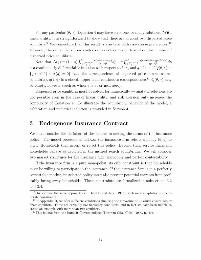
Figure 1 illustrates the resulting solution pairs. Several features of this graph are
qualitatively robust for variations in the parameter values:
• The degenerate equilibrium (q∗ = 1) exists for any coinsurance rate, and for
low coinsurance rates (γ < 5%), it is the only equilibrium.
• A sharp discontinuity occurs where the dispersed price equilibrium emerges,
which is to say that as γ approaches 5%, a new equilibrium at q∗ = 36%
emerges. Nearly two-thirds of the population suddenly begins to request two
quotes.
• At higher rates of coinsurance, two dispersed price equilibria exist. The higher of
these (the upper branch of the curve) is dominated, as mentioned in conjunction
with Proposition 3. Note that the calibration produced a (γ, q) pair on the lower
brach of the curve. The rest of our analysis considers these lower equilibria.
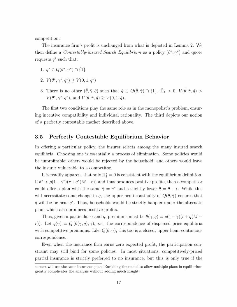
Of course, each of these equilibria result in a different service firm price distribu-
tion. Figure 2 plots the cumulative distribution function F (p) in the equilibrium, for
selected coinsurance rates. At γ = 5%, a wide price distribution suddenly emerges.
As γ increases beyond that point, the distribution increasingly concentrates on lower
prices. However, the largest price reductions occurs between 5% and 15%, and there
is little movement beyond γ = 50%.
22
0.2 0.4 0.6 0.8 1.0Γ
0.2
0.4
0.6
0.8
1.0
q
Figure 1: Insured search equilibrium pairs of fraction of single quotes, q, and coin-surance rate, γ.
1000 1500 2000 2500 3000Price
0.2
0.4
0.6
0.8
1.0
CDF
Figure 2: Equilibrium distribution of prices for selected coinsurance rates: γ = 99%(Solid), γ = 50% (Long Dash), γ = 10% (Short Dash), γ = 6% (Dotted), γ = 5%(DotDash), and γ < 5% (Solid)
23
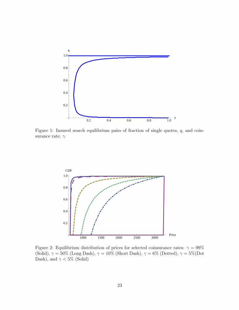
0.0 0.2 0.4 0.6 0.8 1.0Coinsurance Rate
50
100
150
200Ex-Ante Cost
Figure 3: Ex-ante expected costs for each coinsurance rate, γ: insurance premium(solid), out-of-pocket (dotted), and total costs (dashed). (For γ < 5%, total cost isconstant at $363.6. Insurance premium is $363.6(1− γ).)
This dramatic change in the price distribution has a stark effect on the insurance
premiums and out-of-pocket costs paid in each insured search equilibrium. These
are illustrated in Figure 3. In the degenerate equilibrium range, an increase in the
coinsurance rate simply transfers responsibility from the insurance firm to the individ-
ual; the total expected cost remains constant. When the dispersed price equilibrium
emerges at γ = 5%, the reduction in prices is reflected in a discontinuous drop in both
insurance premium and out-of pocket costs. At higher coinsurance rates, premiums
fall and out of pocket costs rise, yet the total cost strictly decreases.
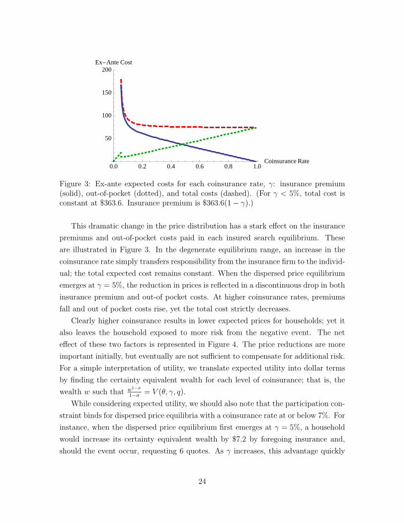
Clearly higher coinsurance results in lower expected prices for households; yet it
also leaves the household exposed to more risk from the negative event. The net
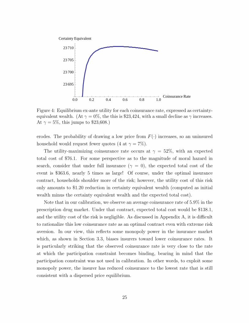
effect of these two factors is represented in Figure 4. The price reductions are more
important initially, but eventually are not sufficient to compensate for additional risk.
For a simple interpretation of utility, we translate expected utility into dollar terms
by finding the certainty equivalent wealth for each level of coinsurance; that is, the
wealth w such that w1−σ
1−σ = V (θ, γ, q).
While considering expected utility, we should also note that the participation con-
straint binds for dispersed price equilibria with a coinsurance rate at or below 7%. For
instance, when the dispersed price equilibrium first emerges at γ = 5%, a household
would increase its certainty equivalent wealth by $7.2 by foregoing insurance and,
should the event occur, requesting 6 quotes. As γ increases, this advantage quickly
24
0.0 0.2 0.4 0.6 0.8 1.0Coinsurance Rate
23 695
23 700
23 705
23 710
Certainty Equivalent
Figure 4: Equilibrium ex-ante utility for each coinsurance rate, expressed as certainty-equivalent wealth. (At γ = 0%, the this is $23,424, with a small decline as γ increases.At γ = 5%, this jumps to $23,608.)
erodes. The probability of drawing a low price from F (·) increases, so an uninsured
household would request fewer quotes (4 at γ = 7%).
The utility-maximizing coinsurance rate occurs at γ = 52%, with an expected
total cost of $76.1. For some perspective as to the magnitude of moral hazard in
search, consider that under full insurance (γ = 0), the expected total cost of the
event is $363.6, nearly 5 times as large! Of course, under the optimal insurance
contract, households shoulder more of the risk; however, the utility cost of this risk
only amounts to $1.20 reduction in certainty equivalent wealth (computed as initial
wealth minus the certainty equivalent wealth and the expected total cost).
Note that in our calibration, we observe an average coinsurance rate of 5.9% in the
prescription drug market. Under that contract, expected total cost would be $138.1,
and the utility cost of the risk is negligible. As discussed in Appendix A, it is difficult
to rationalize this low coinsurance rate as an optimal contract even with extreme risk
aversion. In our view, this reflects some monopoly power in the insurance market
which, as shown in Section 3.3, biases insurers toward lower coinsurance rates. It
is particularly striking that the observed coinsurance rate is very close to the rate
at which the participation constraint becomes binding, bearing in mind that the
participation constraint was not used in calibration. In other words, to exploit some
monopoly power, the insurer has reduced coinsurance to the lowest rate that is still
consistent with a dispersed price equilibrium.
25

In addition to household utility, we may also inquire about total welfare; that is,
the sum of certainty equivalent wealth and firm profits. The latter strictly declines as
coinsurance increases (since the resulting prices have a smaller markup). In fact, total
welfare strictly declines as well. Three important factors produce this result. First,
recall that demand is perfectly inelastic for the repair service; consequently, pricing
above marginal cost creates no deadweight loss in this model. If demand showed some
price sensitivity, households would see greater welfare gains (as coinsurance rises) and
these would offset firm losses. As it is here, however, any price decrease is simply a
transfer from firms to households.
At the same time, there are two costs which cause total welfare to decline. First,
search effort is a real cost. Although households find it individually rational to incur
extra search costs in response to higher coinsurance, this reduces total wealth in
the economy. Second, higher coinsurance rates place more of the risk on households
rather than risk neutral insurers. For the estimated parameters, however, both costs
are minor ($1.6 and $1.2, respectively under the optimal contract).
4.2 Comparative Statics
Since we must numerically solve this model, an important question is how the optimal
contract changes under different parameters. Here we provide these comparative
statics19 as well as the intuition as to why contracts respond in this particular manner.
Much of this can be framed in terms of the positive externality of search: people choose
how many quotes to request based on their private cost and benefit, yet additional
search will reduce prices for all households needing a repair, including those who only
search once.
• Higher cost of requesting a quote: A 1% increase in the cost of search c
results in a 0.3% increase in the optimal coinsurance rate.
As c increases, the second quote request becomes less attractive to households;
if γ were unchanged, a smaller fraction would request two quotes. Yet the
positive externality of search is still as great as before; so γ∗ must increase to
give added incentive for search. Even under the optimal contract, the number
of people requesting two quotes still falls (q∗ rises by 0.9%).
19The comparative statics must also be numerically determined, as implicit differentiation of theequilibrium condition does not yield a sign.
26

• Higher probability of loss: A 1% increase in event probability ρ results in a
0.2% increase in the optimal coinsurance rate.
The probability of loss ρ has very little impact on an individual’s incentive to
search. In Equation 4, note that it does not appear except for its effect on
insurance premiums. However, because the event is more likely, more people
will need repair service, increasing the positive externality. Thus, increasing γ∗
encourages more search (q∗ falls by 0.2%) and lowers prices for all households.
• Higher risk aversion: A 1% increase in risk aversion σ results in a 0.3%
decrease in the optimal coinsurance rate.
As σ increases, it becomes more important to smooth risk for households. Thus,
a lower γ∗ is better for households, even though it results in fewer people search-
ing twice (q∗ falls by 0.4%) and higher prices.
• Higher marginal cost of service: For this comparative static, we shift both
r and M by the same dollar amount, thus keeping the potential markup the
same and only increasing the marginal cost of service. A 1% increase in r results
in a 0.6% decrease in the optimal coinsurance rate.
Although prices are higher as r increases, the expected benefit of search (the
price reduction) is unchanged. On the other hand, the higher expected cost of
the event is equivalent to a reduction in expected wealth. Thus, absolute risk
aversion increases and it is better to forego some price competition in order to
insure households more fully. Thus, γ∗ lowers and fewer people search twice (q∗
rises by 0.8%).
• Higher potential markup: A 1% increase in the maximum allowed price M
results in a 0.15% decrease in the optimal coinsurance rate.
As M increases, households naturally have greater incentive to search because
of the wider price distribution they face. Thus, γ∗ can be lowered and still have
a net result of more people requesting two quotes (q∗ falls by 1.3%). Indeed, the
surprising result is that expected utility under the equilibrium contract rises,
in spite of the higher M ! In our model, M is exogenous, but this suggests that
if the insurer could choose this price cap, contestable markets would encourage
them to loosen it (since it benefits their consumers).
27
The remaining parameter, w, is less interesting. A decrease in w looks very similar
to an increase in r; its only real effect is in increasing absolute risk aversion.
We repeated these computations for a variety of parameter values, and in all cases
these comparative statics maintain the same sign. As γ∗ becomes small, generally the
magnitude of the comparative static diminishes; as γ∗ becomes large, it eventually
hits a corner solution at 1. It is also possible that the degenerate equilibrium with
no coinsurance will eventually dominate the dispersed price equilibrium.
In summary, we can see that a high coinsurance rate is optimal when search costs
or the probability of loss are high, or when risk aversion, cost of provision, or the
maximum allowable price is low. Most of these confirm what one would expect, such
as insuring consumers more fully when they are risk averse or having consumer pay
for a larger fraction of routine care (high ρ) or low-cost prescriptions (low r).
Two results are somewhat surprising: First, higher coinsurance is needed precisely
when it is more costly to obtain price quotes. This continues to be true up until
c > 79, when no insurance is optimal; then once c ≥ 288, full insurance dominates no
insurance. Second, a higher maximum allowable price is actually better for consumers
(after optimally adjusting contracts). This effect becomes small as M increases, but
is still positive when M = w.
5 Measuring Moral Hazard
We quantify the effect of moral hazard in search using the ex-ante expected total cost
of repair, which includes all expenditures, whether paid for by insurance or out-of-
pocket. Here, as in other forms of moral hazard, the presence of insurance will cause
the expected cost to be higher than it would be without.
In Section 3.5, we derived expressions for equilibrium premiums and expected out-
of-pocket expenses (which include search costs). Their sum, the ex-ante total cost, is
ρ(r + 2c+ (M − r − c)q∗) in equilibrium ($76.1 in our calibration). Note that this is
not directly affected by γ or θ; q∗ is the only endogenous variable that directly enters.
Of course, any change in γ or θ that induces a higher fraction of people to search
twice will drive down total cost.
Of course, the policy observed in the data has a much lower coinsurance rate
and consequently a higher fraction of people requesting a single quote. We now
consider the implications of moving from the observed policy to the optimal policy.
28
As a benchmark, suppose we naıvely believed that increasing the coinsurance rate
from 5.9% to 52% would have no effect on consumer search behavior or service firm
pricing. This is to say, if there were no moral hazard in search, the fraction requesting
one quote would hold constant at q = 0.22 regardless of the coinsurance rate. As a
consequence, total expected cost would be ρ(r + 2c + (M − r − c)q) ($138.1 in our
calibration) for any insurance policy; an increase in γ would reduce the insurance
premium, but that would be exactly offset by increases in expected out-of-pocket
costs.
We measure moral hazard, then, as the difference between expected cost in an
environment without moral hazard (i.e. search is fixed at q) and expected cost in an
insured search equilibrium (i.e. at the equilibrium q∗): ρ(M − r − c)|q − q∗| or $62
per household in our calibration.
In our model, two effects contribute to the moral hazard problem. The direct
effect is that, by requesting more quotes, the household has more draws from the
distribution, giving additional chances to obtain a lower quote. This effect was the
sole focus of Dionne (1981), for instance. There is also an indirect (or general equi-
librium) effect: as more households request a second quote, they encourage greater
price competition among the firms, actually lowering the distribution of prices. Our
model is the first to incorporate both effects — and the latter effect is much larger
than the former.
We would like to decompose the two effects. To isolate the direct effect on total
cost, we consider what would happen to total cost (off the equilibrium path) if the
service firm price distribution were fixed while the fraction of households searching
once can vary. In particular, firms set prices as if fraction q of the population searches
once, even though q∗ actually do. The ex-ante total cost EC(q∗, q) in this scenario is:
EC(q∗, q) ≡ ρ q∗
r +q(M − r) ln
(2−qq
)2(1− q)
+ c
+ρ (1− q∗)
2(1− q)(Mq + r − 2qr)− q2(M − r) ln(
2−qq
)2(1− q)2
+ 2c
.
The two large parenthetical terms are the expected price after one quote request (or
two, respectively); note that these only depend on q. The direct effect of moral hazard
29

is then measured as the difference between this cost and the cost when there is no
moral hazard: |ρ(r+ 2c+ (M − r− c)q)−EC(q∗, q)|. Indeed, this equation simplifies
to:ρ|q − q∗|
(q(M − r) ln
(2−qq
)− 2(1− q)((M − r − c)q + c)
)2(1− q)2
.
For the calibration, this amounts to $5.6 of the $62 change in cost; in other words,
9.1% of the change in total cost is due to the direct effect of additional search.
Indeed, we can analytically determine what fraction of the total moral hazard
effect is due to the direct effect: |ρ(r+2c+(M−r−c)q)−EC(q∗,q)|ρ(M−r−c)|q−q∗| . This simplifies to:
S =q(M − r) ln
(2−qq
)− 2(1− q)((M − r − c)q + c)
2(M − c− r)(1− q)2. (7)
Surprisingly, q∗ is cancelled out; the fraction S only depends on the parameters and
the fixed reference point q. S is largest when q ≈ 0.365,20 and is quasi-concave in
q. At its maximum, S ≈ 0.104 − 0.896 cM−c−r . Thus, the direct effect cannot account for
more than 10.4% of the change in total cost; the remaining 89.6% must be due to the
indirect effect. Put another way, the indirect effect is at least 0.8960.104
= 8.6 times as big
as the direct effect, and (if other q are used) potentially more.
6 Conclusion
Our model of moral hazard in search has allowed us to study optimal insurance
contracts when service prices are endogenously determined. Accounting for the firms’
response to consumer search behavior significantly worsens the moral hazard problem.
In our model, insurance companies realize that they can influence the search behavior
with the terms of the contract. In particular, a higher coinsurance rate motivates more
consumers to request a second price quote, which in turn spurs greater competition
among service firms. We find that the indirect effect of search (i.e. greater price
competition among firms) is at least 8.6 times as large as the direct effect (i.e. more
quotes evaluated by households).
The theory also allows us to comment on the industrial organization of the insur-
ance market and its impact on the optimal contract. When the insurance firm is a
20i.e. the solution to S′(q) = 0, which is 2(3− q)(1− q) = (2− q)(1 + q) ln(
2−qq
).
30

monopolist, the equilibrium contract results in full insurance and no price dispersion
among service firms. However, when the insurance market is perfectly contestable,
the threat of competition leads to a contract with a competitive premium and only
partial insurance coverage. This contract also maximizes household expected utility.
Our model could easily be reinterpreted to consider programs for the reimburse-
ment of employee expenses. Company policies range from full reimbursement, which
is equivalent to having no coinsurance, to providing an expense stipend with the em-
ployee claiming any unused residual, similar to 100% coinsurance. Particularly for
business travel, one might reasonably conclude that airline and hotel prices have been
affected by the moral hazard problem of employees making travel arrangements.
From a policy point of view, our work has particular relevance to the debate
regarding health savings accounts (HSAs). HSAs have high deductibles (essentially a
100% coinsurance rate) coupled with full coverage for catastrophic events. Advocates
have cited increased price competition among health providers as one of the benefits
of HSAs, since households covered by such plans will have incentive to shop around (at
least for services that aren’t urgent or likely to exceed the full-coverage threshold).
This paper offers some theoretical foundation for the optimality of that insurance
arrangement. For instance, it is typically optimal to have a 100% coinsurance rate
on routine (i.e. highly likely) and minor (i.e. low marginal cost) health expenses.
When search costs are extremely high (such as when medical attention is urgently
needed) or when the marginal cost of providing the service is quite large (such as
heart surgery), it is often optimal to have a 0% coinsurance rate.
Several extensions to this work would make the model applicable to a broader
range of situations. First and most important is to allow heterogeneity in insurance
coverage, capturing the great variety of private and public insurance plans found co-
existing in the United States. Similarly, we could allow for heterogeneous households,
differing in wealth, cost of search, or probability of loss. This would also enable in-
vestigation into adverse selection issues. The challenge associated with heterogeneity
is that it significantly complicates the procedure of solving for the equilibrium price
distribution, and may render the problem intractable even for numerical solutions.
We would also like to add a quality or product differentiation dimension to the
service firms, since this is the aspect on which most people currently choose their
medical care. Finally, we should note that extension of the present model to a multi-
period environment is crucial to better quantify the magnitude of moral hazard. This
31

would allow future premiums or coinsurance rates to be conditioned on claims paid in
the past, as is the case with most auto insurance. Incorporating this dynamic frame-
work would probably encourage additional search and hence reduce our estimates of
the moral hazard problem.
32

A Data Appendix
The Medical Expenditure Panel Survey (MEPS) is a survey of families and individuals
in the U.S., providing a complete source of data on the cost and use of health care
and health insurance coverage. In this paper, we use the 2005 Prescription Medicine
Event File data that belongs to the Household Component of MEPS. It provides data
from individual households on all their drug purchases, supplemented with data from
their medical providers. An observation is registered each time a prescription is filled,
indicating the prescribed medication (identified with the national drug code (NDC),
which distinguishes among brand names), the date on which the person first used the
medicine, and the amount paid from each potential source of drug coverage (private
insurance, Medicare, out of pocket, etc.).
We focus on prescription drugs because of the homogeneity of the good (within a
given NDC), yet the total price paid for a particular number of pills shows remarkable
dispersion. For instance, a 30 day supply of 10 mg Lipitor pills was sold at anywhere
from $52.60 to $236.69, and as our theory would predict, the distribution is highly
skewed towards lower prices. Figure 5 depicts the observed distribution of prices, as
well as the theoretical distribution found after calibrating q, r, and M .21 Moreover,
prices are not significantly correlated with the source of payment. Moral hazard in
search is a good candidate for explaining price dispersion in this market.
We performed the following calibration on 11 different drugs, listed in Table 2.
Each of these had at least 800 observations in the sample. To maintain homogeneity
within a market, we separate drugs by brand name, dosage, and number of pills
filled in a particular prescription. After calibrating for these, we also calibrate the
model for an aggregation of the drugs (whose values are reported at the bottom of
the table), which are the parameters used in Section 4. The aggregate can be thought
of as insuring against the event that any of these drugs are needed. The calibration
approach is quite similar for an individual drug or for the aggregate.
A.1 Parameters held constant for all drugs
We use the following procedure to set parameter values:
21It is important to note that if some fraction of the population requested more than two quotes,the equilibrium price distribution would be bimodal, with a second spike near M . The observeddata is fully consistent with all households requesting either one or two quotes.
33

0
0
.02
.02
.04
.04
.06
.06
.08
.08
0
0
.02
.02
.04
.04
.06
.06
.08
.08
50
50
100
100
150
150
200
200
250
250
Theoretical Distribution
Theoretical Distribution
Observed Distribution
Observed Distribution
Frequency
Fre
quency
Dollars per 30 pills
Dollars per 30 pills
Figure 5: Observed price distribution (bars) and fitted model price distribution (line)for Lipitor, in annual expenditures.
Wealth (w): We chose w to match the average annual personal income in the data.
We would prefer matching w to wealth, but this data is not available. However, in
the U.S., average wealth and average income are fairly close to each other.
The coinsurance rate (γ): Although the data does report the dollar amount paid
directly by the household rather than by various forms of insurance, it does not
indicate whether the person must contribute a fixed amount for the prescription (a
copay) or a fixed percentage (a coinsurance).22 This is important for our model, since
the former would give no marginal incentive to search if the drug cost is greater than
the copay.
To obtain a reasonable estimate for the average coinsurance rate among house-
holds, we turn to the Kaiser Foundation’s annual study of employer-provided insur-
ance plans (Kaiser Family Foundation, 2006). From their report, one can compute
that across all types of prescription drug policies, 14.9% of employees have a plan
with some form of coinsurance, and among these plans, the average coinsurance rate
22Indeed, even confidential data linking households to their insurance plan lacks details on thecopay or coinsurance associated with prescription drugs.
34

is 26.2% on preferred drugs (which are approved brand-name drugs with no generic
substitute). Another 2% have no coverage (and hence a 100% coinsurance rate). The
remaining 83% have some form of copay, but essentially 0% coinsurance. Thus, we
compute an average coinsurance rate for the population of 5.9%.
Admittedly, this is still not a perfect match to our model, which assumes all
households face the same rate of coinsurance. However, addressing heterogeneity in
the insurance coverage of households would add significant complexity to both the
setup and solution of the model; we thus postpone this for future work. This rough
aggregation is sufficient for our purposes of illustrating the equilibrium behavior.
A.2 Parameters set for each drug
The following parameters were calibrated specifically for each drug. The resulting
values are reported in Table 2.
Percentage of population searching once (q), the marginal cost of production (r),
and the maximum allowable price (M): The values of these three parameters are
calculated from a Maximum Likelihood Estimation that best matches the theoretical
distribution of prices to the observed distribution in the data.
The prices we observe in the data are accepted prices rather than offered prices,
but it is a simple exercise to derive the cumulative distribution of the former using
the cumulative distribution of the latter (expressed in Equation 3 as F (p)). In the
model, q of the population request only one quote and thus accept whatever they
draw; so F (p) of their accepted prices will be at or below price p. The remaining
fraction of the population, 1− q, accepts the lowest of two quotes; thus, if either one
or both of the quotes is below p, we observe an accepted price below p. This happens
1 − (1 − F (p))2 of the time. Hence, the theoretical cumulative distribution function
of accepted prices is
G(p) = qF (p) + (1− q)(1− (1−F (p))2) =
(1 +
(M − p)q2(p− r)
)(1− (M − p)q
2(1− q)(p− r)
).
(8)
This results in a probability density function of
G′(p) =q2(M − r)2
2(1− q)(p− r)3. (9)
35

Hence, the Likelihood Function is
L =n∏i=1
q2(M − r)2
2(1− q)(pi − r)3. (10)
Note that the solution to this problem must satisfy two constraints: first, the
theoretical highest price has to be at least as big as the maximum observed price in
the data: pmax ≤ M . Second, the theoretical lowest price cannot be larger than the
minimum observed price:¯p = r + (M−r)q
2−q ≤ pmin. Therefore, we solve a constrained
optimization problem; typically, both constraints will bind. The results are presented
in Table 2. In the aggregate case, we take the weighted average of these parameters
across all drugs. Note that these parameters are estimated independently of the
others; that is, w, ρ, γ and c are not used in fitting the price data to M , r, and q.
The probability of event occuring (ρ): For each medicine, we used the sample
weights and population estimates to calculate the percentage of the population who
purchased the drug, using this as ρ. For the aggregate case, we set ρ to the fraction
who used any of the listed drugs.
Search cost (c): This last remaining parameter is calibrated by using Equation 4;
that is, households are indifferent between requesting one or two quotes. This must
be solved numerically, but typically has a unique solution for c. The same procedure
is used for the aggregate data, using the average q, r, and M .
Note that we do not try to calibrate for σ. One might consider adjusting this
parameter until the observed coinsurance rate is in fact optimal. Higher risk aver-
sion will typically lower the coinsurance rate in the optimal contract, but not nearly
enough. Even with extreme risk aversion as high as σ = 50, the optimal coinsurance
rate is typically above 20%, far from the observed 5.9% average coinsurance rate.
36

Tab
le2:
Est
imat
edpar
amet
erva
lues
and
exp
ecte
dco
st,
by
dru
g
#of
Obs
Pre
scri
pti
ondru
gρ
(%)
q(%
)r
($)
M($
)c
($)
TC
($)
γ=
0T
C($
)γ
=5.
9γ∗
(%)
TC
($)
γ=γ∗
Ris
kC
ost
($)
2048
Lip
itor
–10
mg
1.4
15.0
52.6
236.
711
.041
.314
.246
9.6
0.1
1930
Lip
itor
–20
mg
1.3
18.8
67.3
334.
017
.452
.818
.946
11.3
0.2
1546
Nor
vasc
–10
mg
0.8
19.9
41.4
186.
29.
619
.07.
351
4.4
0.1
1364
Pre
vaci
d–
30m
g1.
022
.580
.639
4.8
21.6
45.4
17.7
449.
90.
2
1328
Alb
ute
rol
–90
mg
1.2
5.4
7.9
344.
612
.251
.04.
110
01.
50.
0
1197
Pro
tonix
–40
mg
0.9
19.1
72.2
323.
616
.436
.513
.843
8.6
0.1
1191
Flo
nas
e–
0.05
mg
1.6
67.8
26.1
99.1
4.0
18.7
14.3
525.
10.
0
1133
Nor
vasc
–5
mg
0.6
24.9
26.3
134.
77.
610
.14.
163
2.1
0.0
966
Lip
itor
–40
mg
0.6
12.1
73.9
414.
518
.731
.58.
943
6.0
0.1
941
Lex
apro
–10
mg
0.8
22.9
44.7
181.
59.
418
.57.
849
4.8
0.1
890
Adva
irD
iskus
–25
0/50
0.7
26.6
105.
834
4.6
17.0
28.1
13.9
359.
00.
1
Agg
rega
te11
.122
.053
.427
1.7
14.9
363.
613
8.1
5276
.11.
2
•T
Cden
otes
the
hou
sehol
d’s
exp
ecte
dto
tal
cost
ofth
epre
scri
pti
on.
This
isth
esu
mof
the
insu
rance
pre
miu
m,
the
exp
ecte
dco
insu
rance
pay
men
tsou
t-of
-pock
et,
and
exp
ecte
dse
arch
cost
s,to
talingρ(r
+q(M−r)
+(2−q)c)
inth
em
odel
.
•R
isk
Cos
tm
easu
res
the
reduct
ion
inhou
sehol
dw
elfa
refr
omb
eing
only
par
tial
lyin
sure
d(t
hou
ghat
the
opti
mal
γ∗ )
.It
isco
mpute
dasw−CE−TC
,w
her
eCE
isth
ehou
sehol
d’s
cert
ainty
-equiv
alen
tw
ealt
hat
equilib
rium
.
37

B Proofs
B.1 Proposition 2
Proof. For a given q, the expected price from a single quote request is:
¯p+
∫ M
¯p
q(M − p)2(1− q)(p− r)
dp = r +q(M − r) ln
(2−qq
)2(1− q)
.
Similarly, the expected price after two quote requests is:
¯p+
∫ M
¯p
(q(M − p)
2(1− q)(p− r)
)2
dp =2(1− q)(Mq + r − 2qr)− q2(M − r) ln
(2−qq
)2(1− q)2
.
Fraction ρ of the population incurs the loss. Of those, fraction q search once, while
1− q search twice. The insurance company pays 1− γ of the price they are quoted.
Thus, the expected profit is:
ΠI(θ, γ) = θ − (1− γ)ρ
[q
r +q(M − r) ln
(2−qq
)2(1− q)
+
(1− q)
2(1− q)(Mq + r − 2qr)− q2(M − r) ln(
2−qq
)2(1− q)2
]
= θ − ρ(1− γ)(r + q(M − r)).
B.2 Sufficient conditions for the number of equilibria
We have not found an example of risk averse utility in which Equation 4 has more
than two solutions. However, the integrals in this equation make it very hard to prove
that there cannot be more than two solutions. Fortunately, integrals do not appear
in the second derivative of the equilibrium condition, which permits a much better
characterization. Using this approach, we must impose two restrictions on the degree
of curvature of the utility function:
38

Assumption 1. For all w ∈ [w −M − c, w], 45u′(w − c) < u′(w) and
2u′(w) + 9(M − r)γ (u′′(w)− u′′(w − c)) > (M − r)2γ2 (2u′′′(w − c)− u′′′(w)) .
The first condition limits how much marginal utility can change after incurring
the cost of one additional search (with no other change in wealth). The second can
be seen as a restriction on how much the curvature of u can change with the cost of
an additional search. The combination of these ensures that the second derivative of
Equation 4 can only change signs twice. For commonly used utility functions such as
u(w) = w1−σ
1−σ , these conditions are easily satisfied when M and c are small relative to
w.
This condition is sufficient to bound the number of dispersed price equilibria at
two; yet it is definitely not necesary. When chosen parameters and utility functions
violate this assumption (with a very large search cost, for instance), there are typically
no solutions to Equation 4 (because a second quote request never produces enough
additional expected utility to justify the cost).
Proposition 4. Under Assumption 1 with a given (θ, γ), at most two insured search
equilibria with dispersed prices exist.
Proof. Note that∫Mr+
(M−r)q2−q
q(M−r)u(w−θ−c−γp)2(1−q)(p−r)2 dp approaches u(w−θ−c−γM) as q → 1
and u(w − θ − c − γr) as q → 0 (since the probability distributions converge to a
single atom on M and r, respectively). Similarly, the expected utility of searching
twice converges to u(w− θ−2c−γM) and u(w− θ−2c−γr), respectively. Thus, we
know that one bid request is strictly preferred to two bid requests for q near 0 or 1.
The first derivative (w.r.t. q) of the equilibrium condition (Eq. 4) is:
2(1− q)q2(M − r)
(2u(w − θ − 2c− γ
¯p)− u(w − θ − c− γ
¯p)
−q∫ M
¯p
q(M − r)u(w − θ − c− γp)2(1− q)(p− r)2
dp
−(1− q)∫ M
¯p
q2(M − p)(M − r)u(w − θ − 2c− γp)2(1− q)2(p− r)3
dp
).
As q −→ 0, this derivative approaches −∞. As q −→ 1, it approaches 0 from below;
that is, there exists an ε > 0 such that the derivative is strictly negative for all
39
q ∈ [1− ε, 1).
The second derivative (w.r.t. q) of the equilibrium condition is:
4
q3(M − r)(u(w − θ − c− γ
¯p)− u(w − θ − 2c− γ
¯p))
− 4(1− q)γ(2− q)2q2
(2u′(w − θ − 2c− γ
¯p)− u′(w − θ − c− γ
¯p))
At both q = 0 and 1, this derivative is strictly positive. The following equation has
the same sign as the second derivative for each q as well as the same zeros:
D(q) ≡ u(w − θ − c− γ¯p)− u(w − θ − 2c− γ
¯p)
−q(1− q)(M − r)γ(2− q)2
(2u′(w − θ − 2c− γ
¯p)− u′(w − θ − c− γ
¯p)).
Its derivative is:
D′(q) = (M−r)γ(2−q)4
(4q(2− q)u′(w − θ − 2c− γ
¯p)− (2 + q)(2− q)u′(w − θ − c− γ
¯p)
+2q(1− q)(M − r)γ(2u′′(w − θ − 2c− γ
¯p)− u′′(w − θ − c− γ
¯p)) ).
This derivative is initially negative: D′(0) = − (M−r)γ4
u′(w− θ− c− γr) < 0 and ends
positive: D′(1) = (M − r)γ (4u′(w − θ − 2c− γM)− 3u′(w − θ − c− γM)) > 0.
Moreover, since 45u′(w−θ−2c−γ
¯p) < u′(w−θ−c−γ
¯p) by assumption; therefore
4qu′(w− θ− 2c− γ¯p)− (2 + q)u′(w− θ− c− γ
¯p) < 0 for all q ≤ 1
2. Since the second
term of D′ is always negative, this means D′(q) < 0 for all q ≤ 12.
Let A(q) ≡ (2−q)4(M−r)γD
′(q), so A and D′ have the same sign and zeros. Now consider
any q > 12. Assumption 1 gives us:
u′(w − θ − c− γ¯p) +
9(M − r)γ2
(u′′(w − θ − c− γ
¯p)− u′′(w − θ − 2c− γ
¯p))
>(M − r)2γ2
2
(2u′′′(w − θ − 2c− γ
¯p)− u′′′(w − θ − c− γ
¯p)).
Note that the following must also therefore hold since it reduces the right hand side
and increases the left hand side for each q > 12:
40

B(q) ≡ (2− q)3
qu′(w − θ − c− γ
¯p)
+2(M − r)γ((1 + q)(2− q)u′′(w − θ − c− γ
¯p)− 3(2− q)qu′′(w − θ − 2c− γ
¯p))
−2(1− q)q(M − r)2γ2(2u′′′(w − θ − 2c− γ
¯p)− u′′′(w − θ − c− γ
¯p))> 0.
Suppose A(q) ≥ 0 for some q. Then 2(2−q)2B(q) + 2(1−q)
q(2−q)A(q) = A′(q) > 0. Thus,
once A becomes non-negative it is strictly increasing, so there is a unique q ∈(
12, 1]
such that A(q) = 0. Moreover, q is the unique solution in [0, 1] for D′(q) = 0.
Recalling that D(q) > 0 for both q = 0 and 1, then there may be zero, one, or
two solutions to D(q) = 0 because its derivative can only change sign once. Since D
has the same zeros as the second derivative of the equilibrium condition, the latter
also has at most two zeros.
The first derivative of the equilibrium condition is negative near q = 0 and 1.
Suppose there is some interval [q1, q2] for which the first derivative is weakly positive.
Then there exists a q ∈ [q1, q2] such that D(q) = 0, and another q > q2 such that
D(q) = 0. Since the second derivative has at most two zeros, there can only be one
such interval. Thus the first derivative has at most two zeros.
Returning to the equilibrium condition, similar reasoning applies. It is strictly
positive at q = 0 and 1, and if the condition is weakly negative on some interval, then
one zero of the first derivative lies within that interval and another lies above that
interval. Hence, only one such interval exists, and the equilibrium condition can only
hold with equality up to twice.
41

References
Arrow, Kenneth. (1963) “Uncertainty and the Welfare Economics of Medical Care,”
American Economic Review 53, 941-973.
Burdett, Kenneth, and K. Judd. (1983) “Equilibrium Price Dispersion,” Econometrica
51, 955-969.
Crew, Michael. (1969) “Coinsurance and the Welfare Economics of Medical Care,”
American Economic Review 59, 906-908.
Dionne, Georges. (1981) “Moral Hazard and Search Activity,” Journal of Risk and
Insurance 48, 422-434.
Dionne, Georges. (1984) “Search and Insurance,” International Economic Review 25,
357-367.
Ehrlich, Isaac, and G. Becker. (1972) “Market Insurance, Self-Insurance, and Self-
Protection,” Journal of Political Economy 80, 623-648.
Feldstein, Martin. (1970) “The Rising Price of Physicians’ Services”Review of Eco-
nomics and Statistics 52, 121-133 .
Feldstein, Martin. (1971) “Hospital Costs Inflation: A Study in Non-Profit Price
Dynamics”American Economic Review 61, 853-872 .
Feldstein, Martin. (1973) “The Welfare Loss of Excess Health Insurance”Journal of
Political Economy 81, 251-280.
Gaynor, Martin, D. Haas-Wilson, and W. Vogt. (2000) “Are Invisible Hands Good
Hands? Moral Hazard, Competition, and the Second-Best in Health Care Markets,”
Journal of Political Economy 108, 992-1005.
Kaiser Family Foundation and Health Research Educational Trust. (2006) “Section
9: Prescription Drug and Mental Health Benefits,” Employer Health Benefits, 2006
Annual Report, 115-124.
Ma, Ching-To, and T. McGuire. (1997) “Optimal Health Insurance and Provider
Payment,” American Economic Review 87, 685-704.
42
Manning, Richard, and P. Morgan. (1982) “Search and Consumer Theory,” Review
of Economic Studies 49, 203-216.
Mas-Colell, Andreu. (1990) The Theory of General Economic Equilibrium: A Differ-
entiable Approach. Cambridge: Cambridge Press.
Morgan, Peter, and R. Manning. (1985) “Optimal Search,” Econometrica 53, 923-
944.
Nell, Martin, A. Richter, and J. Schiller. (2008) “When Prices Hardly Matter: In-
complete Insurance Contracts and Markets for Repair Goods,” European Economic
Review, forthcoming.
Pauly, Mark. (1968) “The Economics of Moral Hazard: Comment,” American Eco-
nomic Review 58, 531-537.
Pavcnik, Nina. (2002) “Do pharmaceutical prices respond to patient out-of-pocket
expenses?”Rand Journal of Economics 33, 469-487.
Smith, Vernon. (1968) “Optimal Insurance Coverage,” Journal of Political Economy
76, 68-77.
Sorensen, Alan. (2000) “Equilibrium Price Dispersion in Retail Markets for Prescrip-
tion Drugs,” Journal of Political Economy 108, 833-850.
Zeuckhauser, Richard. (1970) “Medical Insurance: A Case Study of the Tradeoff
between Risk Spreading and Appropriate Incentives,” Journal of Economic Theory
10, 10-26.
43