SEA SURFACE SALINITY RETRIEVAL BASED ON LEVENBERG

MARQUARDT ALGORITHM USING SATELLITE DATA

NOORLIDA BINTI ABD RAHIM

UNIVERSITI TEKNOLOGI MALAYSIA

i

SEA SURFACE SALINITY RETRIEVAL BASED ON LEVENBERG

MARQUARDT ALGORITHM USING SATELLITE DATA

NOORLIDA BINTI ABD RAHIM

A thesis submitted in fulfilment of the

requirements for the award of the degree of

Master of Science (Remote Sensing)

Faculty of Geoinformation and Real Estate

Universiti Teknologi Malaysia

AUGUST 2014

iii

Dedicated to my beloved mother and father,

My beloved one

My beloved siblings....

And Special Appreciation to

All lecturers from Department of Remote Sensing

Thanks for all the support...

iv

ACKNOWLEDGEMENT

In the name of ALLAH SWT, I would like to express my gratefulness and

most heartfelt thanks to Him for giving me strength to successfully complete my

study. First and foremost, I wish to express my gratitude to my academic supervisors

Dr. Mohd Nadzri bin Md Reba and Prof. Dr. Mohd Ibrahim Seeni Mohd for their

guidance, support and encouragement during my study.

I would like to thank my parents, Abd Rahim bin Mohd Amin and Zalekha

binti Endut to whom I dedicate this work for their love and constant support. My

special thanks to my husband, Aminuddin bin Mohd Noor whose patient and love

enabled me to complete this work. Thanks to other individuals who have contributed

to the success of this report whether directly or indirectly.

v

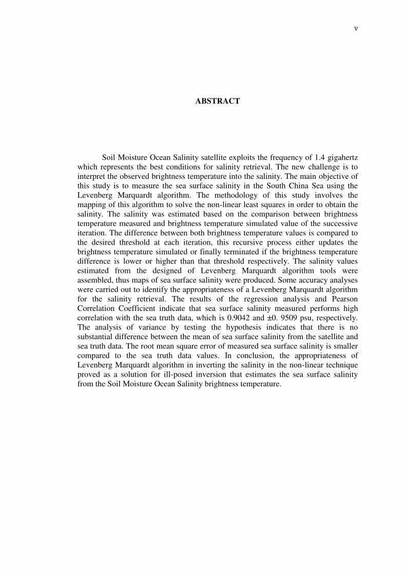
ABSTRACT

Soil Moisture Ocean Salinity satellite exploits the frequency of 1.4 gigahertz

which represents the best conditions for salinity retrieval. The new challenge is to

interpret the observed brightness temperature into the salinity. The main objective of

this study is to measure the sea surface salinity in the South China Sea using the

Levenberg Marquardt algorithm. The methodology of this study involves the

mapping of this algorithm to solve the non-linear least squares in order to obtain the

salinity. The salinity was estimated based on the comparison between brightness

temperature measured and brightness temperature simulated value of the successive

iteration. The difference between both brightness temperature values is compared to

the desired threshold at each iteration, this recursive process either updates the

brightness temperature simulated or finally terminated if the brightness temperature

difference is lower or higher than that threshold respectively. The salinity values

estimated from the designed of Levenberg Marquardt algorithm tools were

assembled, thus maps of sea surface salinity were produced. Some accuracy analyses

were carried out to identify the appropriateness of a Levenberg Marquardt algorithm

for the salinity retrieval. The results of the regression analysis and Pearson

Correlation Coefficient indicate that sea surface salinity measured performs high

correlation with the sea truth data, which is 0.9042 and ±0. 9509 psu, respectively.

The analysis of variance by testing the hypothesis indicates that there is no

substantial difference between the mean of sea surface salinity from the satellite and

sea truth data. The root mean square error of measured sea surface salinity is smaller

compared to the sea truth data values. In conclusion, the appropriateness of

Levenberg Marquardt algorithm in inverting the salinity in the non-linear technique

proved as a solution for ill-posed inversion that estimates the sea surface salinity

from the Soil Moisture Ocean Salinity brightness temperature.

vi

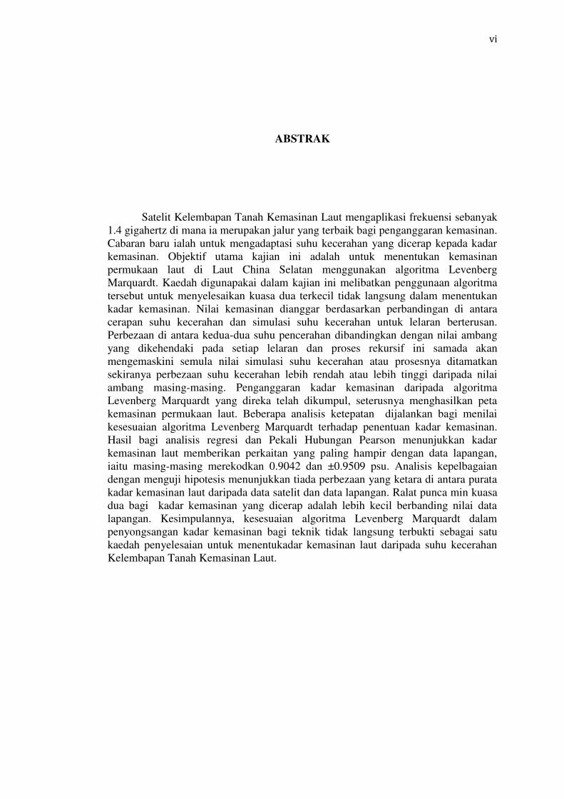
ABSTRAK

Satelit Kelembapan Tanah Kemasinan Laut mengaplikasi frekuensi sebanyak

1.4 gigahertz di mana ia merupakan jalur yang terbaik bagi penganggaran kemasinan.

Cabaran baru ialah untuk mengadaptasi suhu kecerahan yang dicerap kepada kadar

kemasinan. Objektif utama kajian ini adalah untuk menentukan kemasinan

permukaan laut di Laut China Selatan menggunakan algoritma Levenberg

Marquardt. Kaedah digunapakai dalam kajian ini melibatkan penggunaan algoritma

tersebut untuk menyelesaikan kuasa dua terkecil tidak langsung dalam menentukan

kadar kemasinan. Nilai kemasinan dianggar berdasarkan perbandingan di antara

cerapan suhu kecerahan dan simulasi suhu kecerahan untuk lelaran berterusan.

Perbezaan di antara kedua-dua suhu pencerahan dibandingkan dengan nilai ambang

yang dikehendaki pada setiap lelaran dan proses rekursif ini samada akan

mengemaskini semula nilai simulasi suhu kecerahan atau prosesnya ditamatkan

sekiranya perbezaan suhu kecerahan lebih rendah atau lebih tinggi daripada nilai

ambang masing-masing. Penganggaran kadar kemasinan daripada algoritma

Levenberg Marquardt yang direka telah dikumpul, seterusnya menghasilkan peta

kemasinan permukaan laut. Beberapa analisis ketepatan dijalankan bagi menilai

kesesuaian algoritma Levenberg Marquardt terhadap penentuan kadar kemasinan.

Hasil bagi analisis regresi dan Pekali Hubungan Pearson menunjukkan kadar

kemasinan laut memberikan perkaitan yang paling hampir dengan data lapangan,

iaitu masing-masing merekodkan 0.9042 dan ±0.9509 psu. Analisis kepelbagaian

dengan menguji hipotesis menunjukkan tiada perbezaan yang ketara di antara purata

kadar kemasinan laut daripada data satelit dan data lapangan. Ralat punca min kuasa

dua bagi kadar kemasinan yang dicerap adalah lebih kecil berbanding nilai data

lapangan. Kesimpulannya, kesesuaian algoritma Levenberg Marquardt dalam

penyongsangan kadar kemasinan bagi teknik tidak langsung terbukti sebagai satu

kaedah penyelesaian untuk menentukadar kemasinan laut daripada suhu kecerahan

Kelembapan Tanah Kemasinan Laut.

vii

TABLE OF CONTENTS

CHAPTER

TITLE PAGE

1

2

DECLARATION

DEDICATION

ACKNOWLEDGEMENT

ABSTRACT

ABSTRAK

TABLE OF CONTENTS

LIST OF TABLES

LIST OF FIGURES

LIST OF SYMBOLS

LIST OF ABBREVIATIONS

LIST OF APPENDICES

INTRODUCTION

1.1 Background of the Study

1.2 Problem Statement

1.3 Objectives

1.4 Scope of Study

1.5 Significance of Study

1.6 Study Area

LITERATURE REVIEW

2.1 Introduction

2.2 Soil Moisture and Ocean Salinity (SMOS) Mission

ii

iii

iv

v

vi

vii

x

xi

xiii

xv

xvi

1

4

5

5

6

7

9

10

viii

3

4

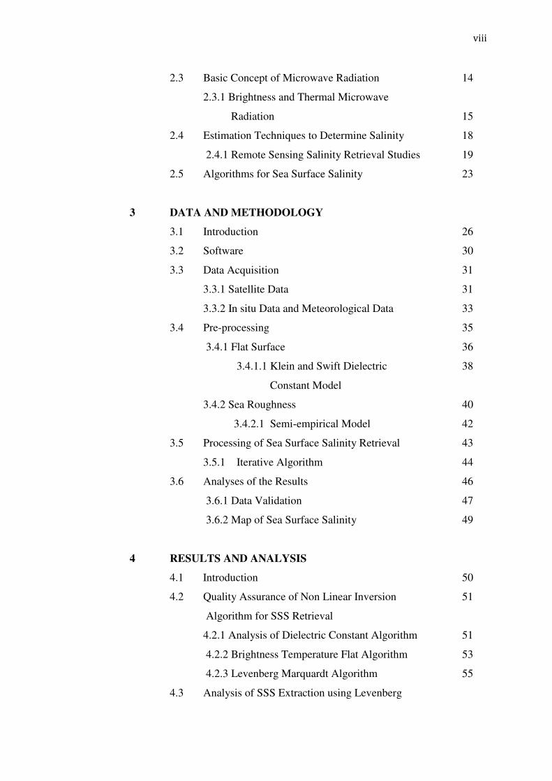
2.3 Basic Concept of Microwave Radiation

2.3.1 Brightness and Thermal Microwave

Radiation

2.4 Estimation Techniques to Determine Salinity

2.4.1 Remote Sensing Salinity Retrieval Studies

2.5 Algorithms for Sea Surface Salinity

DATA AND METHODOLOGY

3.1 Introduction

3.2 Software

3.3 Data Acquisition

3.3.1 Satellite Data

3.3.2 In situ Data and Meteorological Data

3.4 Pre-processing

3.4.1 Flat Surface

3.4.1.1 Klein and Swift Dielectric

Constant Model

3.4.2 Sea Roughness

3.4.2.1 Semi-empirical Model

3.5 Processing of Sea Surface Salinity Retrieval

3.5.1 Iterative Algorithm

3.6 Analyses of the Results

3.6.1 Data Validation

3.6.2 Map of Sea Surface Salinity

RESULTS AND ANALYSIS

4.1 Introduction

4.2 Quality Assurance of Non Linear Inversion

Algorithm for SSS Retrieval

4.2.1 Analysis of Dielectric Constant Algorithm

4.2.2 Brightness Temperature Flat Algorithm

4.2.3 Levenberg Marquardt Algorithm

4.3 Analysis of SSS Extraction using Levenberg

14

15

18

19

23

26

30

31

31

33

35

36

38

40

42

43

44

46

47

49

50

51

51

53

55

ix

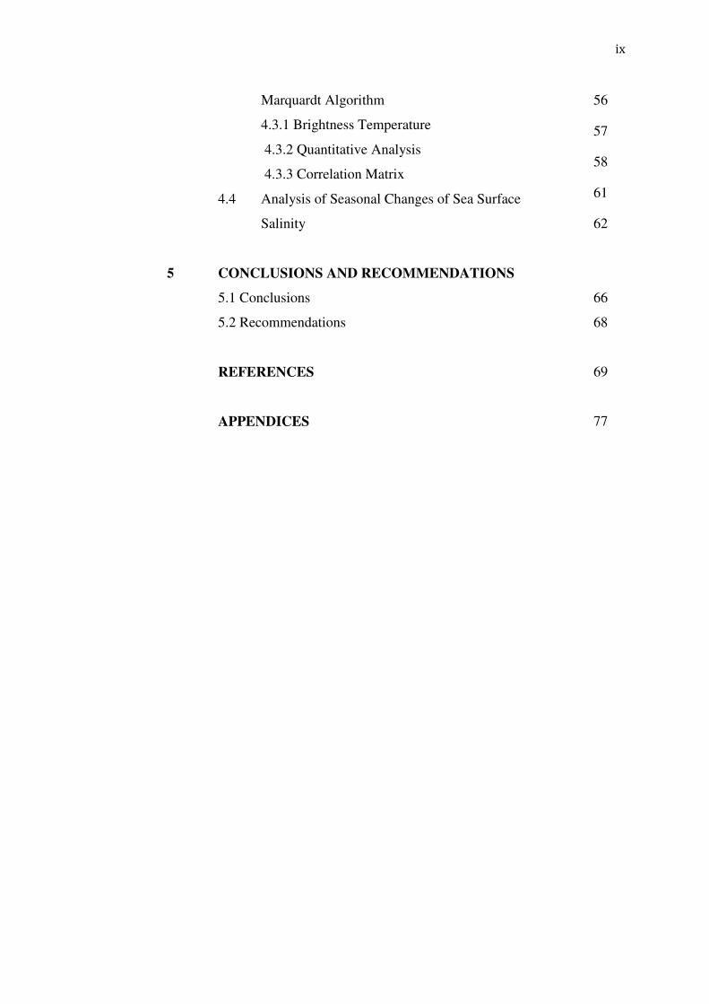
Marquardt Algorithm

4.3.1 Brightness Temperature

4.3.2 Quantitative Analysis

4.3.3 Correlation Matrix

4.4 Analysis of Seasonal Changes of Sea Surface

Salinity

56

57

58

61

62

5

CONCLUSIONS AND RECOMMENDATIONS

5.1 Conclusions

5.2 Recommendations

REFERENCES

APPENDICES

66

68

69

77

x

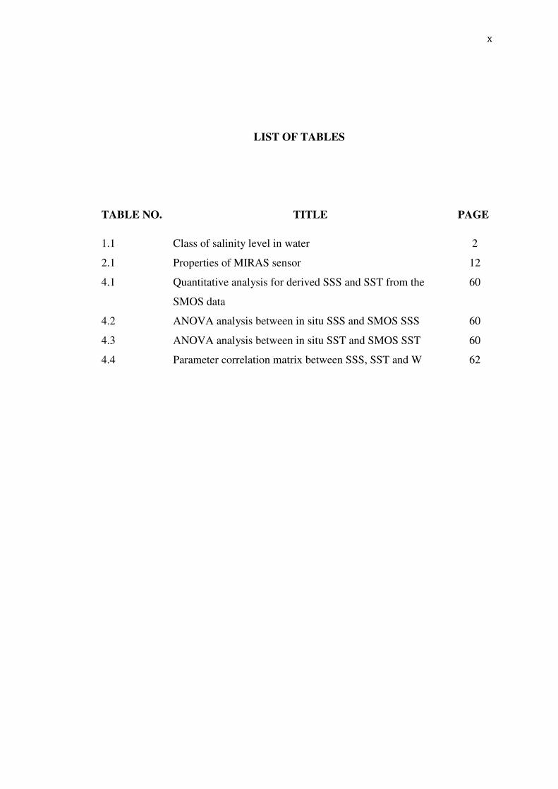
LIST OF TABLES

TABLE NO. TITLE PAGE

1.1

2.1

4.1

4.2

4.3

4.4

Class of salinity level in water

Properties of MIRAS sensor

Quantitative analysis for derived SSS and SST from the

SMOS data

ANOVA analysis between in situ SSS and SMOS SSS

ANOVA analysis between in situ SST and SMOS SST

Parameter correlation matrix between SSS, SST and W

2

12

60

60

60

62

xi

LIST OF FIGURES

FIGURE NO. TITLE PAGE

1.1

1.2

2.1

2.2

2.3

2.4

3.1

3.2

3.3

3.4

3.5

3.6

4.1

4.2

4.3

4.4

4.5

The hydrologic water cycle

Location map of the study area

Soil Moisture and Ocean Salinity (SMOS) satellite

SMOS alias-free FOV

Sensitivity of several parameters to frequency

The black body - brightness density as a function of the

temperature wavelength

Flowchart of SMOS Data Processing

Development of the SSS Processing Tool

Three levels of Class II aperture 4 hexagon hierarchies

defined on a single triangle face

One snapshot from the SMOS L1C product

The half-orbit overpass from the SMOS L1C product with

different incidence angles

Map of in situ points distributions

The plot of dielectric constant vs temperature

Brightness temperature dependence on the observation

angle for a perfectly flat sea surface of horizontal and

vertical polarization

The sum of the squared errors (χ2) as a function of SST and

SSS

Plot of brightness temperature versus incidence angle

Regression plot between the estimated SSS from SMOS

and in situ data

3

8

10

11

12

17

28

29

32

32

33

34

52

54

55

57

58

xii

4.6

4.7

4.8

Regression plot between the estimated SST from SMOS

and in situ data

Map of SSS estimation from SMOS satellite during south

west monsoon

Map of SSS estimation from SMOS satellite during north

east monsoon

59

64

65

xiii

LIST OF SYMBOLS

B - Radiance [Wm-2sr-1]

Ft - The Power Flux Emitted [W.sr-1]

At - Unit of Surface [m2]

Ar - The Effective Area of the Antenna [m2]

R - The Distance between the Antenna and the

Radiating Target [m]

Ωt - The Transmitting Antenna [.]

P - Power [Watts]

Δf - Bandwidth of the Receiver [Hertz]

f - Frequency [Hertz]

h - Constant of Planck (6.63x10-34

Js)

T - Absolute Physical Temperature [K]

c - Speed of Light [ms-1

]

Bbb - Brightness of a Blackbody [K]

e - Emissivity [.]

R - Fresnel Power Reflection Coefficient Dependent on

the Polarization. [.]

Tb - Brightness Temperature [K]

Tb,flat - Brightness Temperature of a Flat Sea Surface [K]

Tb,rough - Contribution of Sea Surface Roughness [K]

θ - Incidence Angle [degree]

SST - Sea Surface Temperature [°C]

SSS - Sea Surface Salinity [psu]

Prough - Parameter Used To Characterize the Roughness

Γ - Reflectivity [.]

Rp - Fresnel Reflection Coefficient At Polarization p

xiv

ε - Dielectric Constant of Seawater [.]

ε∞ - The Dielectric Constant at Infinite Frequency [.]

εs - The Static Dielectric Constant [.]

ω - Radian Frequency [Hertz]

- The Relaxation Time [seconds]

i - Imaginary Number [.]

- The Ionic Conductivity [mhos/meter]

ε0 - The Permittivity of Free Space [farads/meter]

W10 - Wind Speed Below than 10 m/s [m/s]

χ2 - The Sum of Squared Difference between Tb meas and

Tb sim

Tb,meas - Measured Brightness Temperature [K]

Tb,sim - Simulated Brightness Temperature [K]

N - Number of SMOS Measurements along a Dwell Line

p - Variance of The Expected Error of the Reference

Values

xv

LIST OF ABBREVIATIONS

AMSR-E - Advanced Microwave Scanning Radiometer for EOS

CCSDS - Consultative Committee for Space Data Systems

CDOM - Color Dissolved Organic Matter

CEOS - Committee on Earth Observation Satellites

DGG - Discrete Global Grid

ECS - East China Sea

EEZ - Exclusive Economic Zone

EMR - Electromagnetic Radiation

ENSO - El-Nino Southern Oscillation

E-P - Evaporation minus Precipitation

ESA - European Space Agency

FOV - Field of View

ISEA - Icosahedral Synder Equal Area

L1C - SMOS Level 1C data

MIRAS - Microwave Imaging Radiometer Using Aperture

Synthesis

SMOS - Soil Moisture and Ocean Salinity

SSS - Sea Surface Salinity

SSA - Small Slope Approximation Model

SST - Sea Surface Temperature

SWH - Significant Wave Height

W - Wind Speed

WISE - Wind and Salinity Experiments

xvi

LIST OF APPENDICES

APPENDIX TITLE PAGE

A

B

C

In situ Data of Sea Surface Salinity

In Situ Data of Sea Surface Temperature

Source Code of Sea Surface Salinity Program

77

78

79

1

CHAPTER 1

INTRODUCTION

1.1 Background of the Study

Study on ocean becomes significant as the ocean covers almost 71 percent of

the earth’s surface and it has larger influence and capability in transporting energy.

As a result, this imposes knowledge on coastal characteristics and climate to be

improved. Salinity is dissolved salt or literally defined as the total amount of

dissolved solids in the units of 1000 grams. Interaction between lattices and water

molecules induces salinity to form the ion which is the charged molecules. By the

presence of molecule charges, salinity can be determined by seawater's conductivity.

The main salt ions contributed to the seawater element are chlorine, sodium,

sulphate, magnesium, calcium, and potassium. Seawater also contains some types of

dissolved gases such as carbon dioxide, nitrogen, and oxygen.

In the climatological aspect, salinity observation becomes an integral part of

global ocean observations designed ultimately to monitor interannual to interdecadal

processes as of the idea is to understand uncertainties of El-Nino Southern

Oscillation (ENSO) forecasting, global warming and other climate variations

(Lagerloaf et al., 1995). In fisheries, the lower salinity level that originated from the

2

fresh water end turns sea grass blades to yellow and thus this adversely impacts the

breeding ground for fish, prawns and other aquatic lives (Thorhaug et al., 2006).

Salinity plays an important role in the earth’s water cycle in which it

subsequently affects the weather and climate by means of temperature salinity that

drives the ocean currents. The change in salinity is mainly caused by the additional

or removal of freshwater from land. The salinity of sea water is normally about 30 to

35 psu (practical salinity unit) in open ocean but tends to be variable in coastal water

coming from the fresh water output, tidal fluctuations and etc (Thorhaug et al.,

2006). Several studies have reported that the reflectance spectra of certain seagrass

species indicating the physiology of the seagrass are strongly and significantly

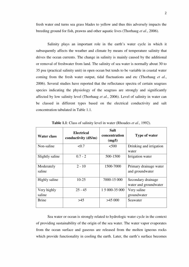
affected by low salinity level (Thorhaug et al., 2006). Level of salinity in water can

be classed in different types based on the electrical conductivity and salt

concentration tabulated in Table 1.1.

Table 1.1: Class of salinity level in water (Rhoades et al., 1992).

Water class Electrical

conductivity (dS/m)

Salt

concentration

(mg/l)

Type of water

Non-saline <0.7 <500 Drinking and irrigation

water

Slightly saline 0.7 - 2 500-1500 Irrigation water

Moderately

saline

2 - 10 1500-7000 Primary drainage water

and groundwater

Highly saline 10-25 7000-15 000 Secondary drainage

water and groundwater

Very highly

saline

25 - 45 1 5 000-35 000 Very saline

groundwater

Brine >45 >45 000 Seawater

Sea water or ocean is strongly related to hydrologic water cycle in the context

of providing sustainability of the origin of the sea water. The water vapor evaporates

from the ocean surface and gaseous are released from the molten igneous rocks

which provide functionality in cooling the earth. Later, the earth’s surface becomes

3

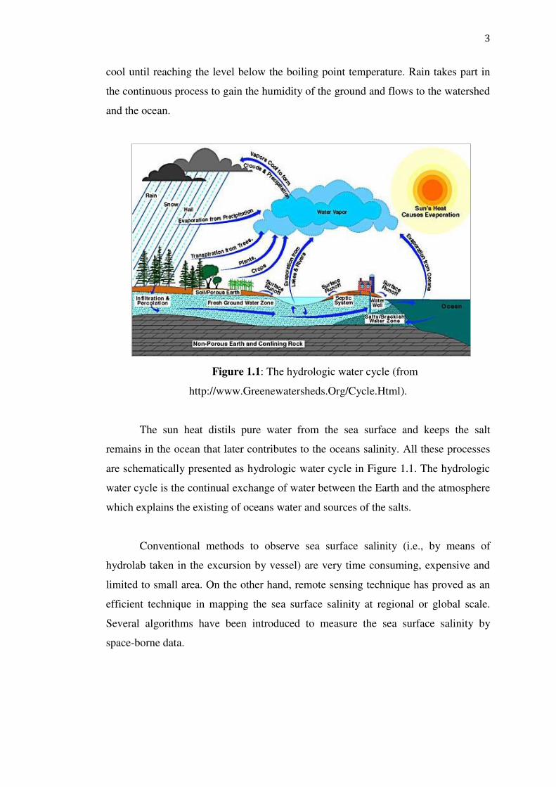
cool until reaching the level below the boiling point temperature. Rain takes part in

the continuous process to gain the humidity of the ground and flows to the watershed

and the ocean.

Figure 1.1: The hydrologic water cycle (from

http://www.Greenewatersheds.Org/Cycle.Html).

The sun heat distils pure water from the sea surface and keeps the salt

remains in the ocean that later contributes to the oceans salinity. All these processes

are schematically presented as hydrologic water cycle in Figure 1.1. The hydrologic

water cycle is the continual exchange of water between the Earth and the atmosphere

which explains the existing of oceans water and sources of the salts.

Conventional methods to observe sea surface salinity (i.e., by means of

hydrolab taken in the excursion by vessel) are very time consuming, expensive and

limited to small area. On the other hand, remote sensing technique has proved as an

efficient technique in mapping the sea surface salinity at regional or global scale.

Several algorithms have been introduced to measure the sea surface salinity by

space-borne data.

4

1.2 Problem Statement

Traditional methods that extract salts directly from the ocean are very time

consuming, expensive and limited to small area coverage. For instance, the

estimation of net Evaporation minus Precipitation (E-P) has high correlation with sea

surface salinity and therefore is used to relatively estimate the sea surface salinity.

Even though the net E-P provides better understanding of the thermohaline

circulation and later this technique helps to improve the estimation of latent heat

flux, E-P measurement imposes massive manpower, high time consuming and very

costly.

Sea surface salinity retrieval by remote sensing technique proved as an

efficient technique in mapping the salinity at regional or global scale. In the context

of Malaysian coastal waters, focus more on the sea-truthing than satellite-based

measurements are mainly reported. The satellite derived sea surface salinity was

majorly formulated by means of optical bands at which interferences by weather,

cloud covers and atmospheric induced error are regularly encountered. There is also

concern on the impact of seasonal monsoon towards the sea surface salinity

particularly at the east coast of Malaysia where the study on impact is necessary for

biological production and ocean ecology studies.

Most of the satellite derived sea surface salinity was obtained by optical

remote sensing data though this approach has disadvantages of interferences

produced by atmospheric condition, weather and cloud covers. This is not a case for

the microwave radiometer type satellite called Soil Moisture and Ocean Salinity

(SMOS) which has been deployed in space in 2009 by which high degree of ocean

salinity and soil moisture are retrieved using microwave sensor. Yet, the salinity

product estimated from the Microwave Imaging Radiometer Using Aperture

Synthesis (MIRAS) have yet been calibrated and validated as this 1.4GHz L-band

sea surface salinity variant is ill-pose solution. As a result, high order non linear

solution is needed and provides complicated solution.

5

1.3 Objectives

The aim of this study is to measure the sea surface salinity using the SMOS

data over the South China Sea. Therefore, the objectives of this study are:

1. To develop a tool for the SMOS sea surface salinity retrieval based on a

non-linear inversion algorithm using the ocean surface brightness

temperature data.

2. To validate the SMOS sea surface salinity retrieval over the coastal water of

Malaysia using the corresponding in-situ measurements.

3. To map the ocean salinity distribution of South China Sea from SMOS data.

4. To determine the impact of seasonal monsoon on the estimated SMOS sea

surface salinity.

1.4 Scope of Study

The scopes of this study are as follows,

1. Soil Moisture and Ocean Salinity (SMOS) data providing sea surface salinity

information within large area of 35 kilometre and revisiting time of 3 days

with accuracy between 0.5 to 1.5 psu for a single observation is used as the

primary data. Level 1C data is projected on an Icosahedral Synder Equal Area

(ISEA 4H9) grid provides a uniform inter cell distance of 15 km.

2. Klein and Swift model (1977) and semi-empirical models are considered to

compute the brightness temperature in both conditions of flat sea surface and

rough sea surface as those models provide systematic and straight ward

estimation procedures.

6

3. Levenberg Marquardt technique is chosen to solve for the non-linear

optimization and inversion on the SMOS brightness temperature pixels

because the technique provides simultaneous estimation of sea surface

salinity, sea surface temperature and wind speed.

4. Sea truth data of sea surface salinity and sea surface temperature were used

for algorithm validation and the fieldwork was carried out in the coastal water

of east coast of Peninsular Malaysia on June 2008 and June 2009. Besides

that, some sea truth data were obtained from the related agencies namely

Universiti Malaysia Terengganu (UMT) and Southeast Asian Fisheries

Development Center (SEAFDEC).

5. For calibration and validation of the SMOS data, regression analysis

provides better overview on the accuracy of SMOS derived sea surface

salinity.

1.5 Significance of Study

This is the first study of SMOS data application in the Malaysia coastal water

that involves extensive data processing (i.e., SMOS data acquisition, brightness

temperature estimation and validation) and development of iterative non-linear

inversion algorithm. The SMOS mission is dedicated to continuously measure the

ocean salinity and soil moistures over the globe at the higher degree of accuracy in

space and time. This study would serve to the salinity mapping over coastal water in

east coast Peninsular Malaysia and give benefit to fisheries, aquaculture and habitats

for coral reef and sea grass. Salinity affects water density that controls the sinking of

water and the patterns of evaporation over the ocean. This would therefore improve

the knowledge of the water cycle and thus gives better understanding of climate

change. Salinity information helps to constrain the hydrological cycle and by

7

incorporating high degree of accuracy of salinity may improve ocean circulation

modelling and data assimilation (Yueh et al., 2000).

Validation and calibration of SMOS salinity product may serve to local

satellite mapping in order to improve the accuracy of data product. In this case,

discrepancy of satellite salinity product is reduced so that increases its data reliability

in space and time. As result, high accuracy remote sensing data offer more effective

salinity mapping technique and more cost efficiency covering large ocean areas than

that of conventional ones. Study on the impact of seasonal monsoon to the salinity

distribution give significance overview for the ocean bio geochemical identification

namely shellfish productivity, aquaculture, ice melt process, major river run-off

events and fish location dependent parameters (Castillo et al., 1996; Morita et al.,

2001).

1.6 Study Area

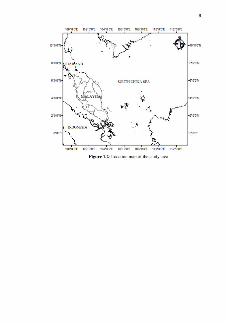
The study area is in the South China Sea as shown in Figure 1.2. The area

covered from 2°30’σ and 103°00’E to 6°00’σ and 105°00’E that governs open

seawater with low and high salinity range. There are various surrounding marine

resources and habitats that rich with coral reefs, sea grass and seaweeds and therefore

this area is also known as the Exclusive Economic Zone (EZZ). The change in

salinity in turn affects the coral reefs, sea grass and seaweed habitats that eventually

intervenes the growth and life of fish, prawns, sea cucumber and other marine

resources. The South China Sea is the marginal sea and connects to the East China

Sea (ECS), the Pacific Ocean in northern and also links with the Java Sea and the

Sulu Sea in the south. The South China Sea is one of the busiest ocean routes and

networks for ships.

8

Figure 1.2: Location map of the study area.

69

REFERENCES

Ahn Y. H., Shanmugam P., Moon J.E.and Ryu J.H. (2008). Satellite Remote Sensing

of a Low-Salinity Water Plume in the East China Sea. European Geosciences

Union 2008: 2019-2035.

Altman D.G. and Schulz, K.F., (2001). Statistics Notes: Concealing treatment

allocation in randomized trials. British Medical Journal 323: 446-447.

Ammar A., Labroue S., Obligis E., Mejia C. E., Crepon M. and Thiria S. (2008). Sea

Surface Salinity Retrieval for the SMOS Mission Using Neural Networks.

IEEE Transaction on Geoscience and Remote Sensing, Vol. 46, No. 3, March

2008.

Binding C.E., Bowers D.G. (2003). Measuring the Salinity of Clyde Sea from

Remotely Sensed Ocean Color. Elsvier Science. Estuarine, Coastal and Shelf

Science 57 (2003) 605-611.

Blanch S. and Aguasca A. (2004). Seawater Dielectric Permittivity Model From

Measurements at L-Band. Proceedings of IGARSS 2004, Alaska.

Burrage D., Wesson J. and M., (2008). Deriving Sea Surface Salinity and Density

Variations From Satellite and Aircraft Microwave Radiometer Measurements:

Application to Coastal Plumes Using STARRS. IEEE Transactions on

Geosciences and Remote Sensing, 46 (3), pp: 765- 785.

Camps A., Corbella I., Vall llossera M., Duffo N., Torres F., Villarino R., Enrique

L., Julbe F., Font J., Julia A., Gabarro C., Etcheto J., Boutin J., Weill A.,

Rubio E., Caselles V., Wursteisen P., Martin-Neira M. (2003). L-Band Sea

70

Surface Emissivity: Preliminary Results of the Wise-2000 Campaign and Its

Application to Salinity Retrieval in the SMOS Mission, Radioscience, 38 (4),

MAR 36-3.

Camps A., Font J., Vall-llossera M., Gabarro C., Corbella I., Duffo N., Torres F.,

Blanch S., Aguasca A., Villarino R., Enrique L., Miranda J.J., Arenas J.J., Julia

A., Etcheto J., Caselles V., Weill A., Boutin J., Contardo S., Niclos R., Rivas

R., Reising S.C., Wursteisen P., Berger M. and Martin-Neira, M. (2004). The

WISE 2000 and 2001 Campaigns in Support of the SMOS Mission: Sea

Surface L-band Brightness Temperature Observations and their Application to

Multi-Angular Salinity Retrieval, IEEE Trans. Geosci. and Remote Sens.,

42(4), 804-823.

Castillo J., Barbieri M.A., and Gonzales A. (1996). Relationship between Sea

Surface Temperature, Salinity and Pelagic Fish Distribution off Northern

Chile. ICES Journal of Marine Science 53(2):139-146.

Corbella I., Torres F., Duffo N., Gonzalez V., Camps A. and Vall-llossera, M.

(2008). Fast Processing Tool for SMOS Data. International Geoscience and

Remote Sensing Symposium (IGARSS) 2008. IEEE International. 2 (1), art no.

4779204, pp II-1152 - II-1155.

Debye, P. (1929). Polar Molecules. Dover Publication. New York: Reinhold

Publishing Corp.

Delwart S., Petitcolin F., and SMOS Team (2006). SMOS SSS L2 Algorithm

Theoretical Baseline Document ICM-CSIC LOCEAN/SA/CETP IFREMER,

2006.

Dinnat E. P., Boutin J., Caudal G. and Etcheto J. (2003). Issues Concerning the Sea

Emissivity Modeling at L Band for Retrieving Surface Salinity. Radio Sci.,

Vol. 38, no. 4, 8060, 2003, DOI:10.1029/2002RS002637.

71

Droppelman, J.D., Mennella R.A. and Evans D.E. (1970). An Airborne Measurement

of the Salinity Variations of the Mississippi River Outflow. J. Geophys. Res.,

75, 5909 5913.

Durden S. L., and Vesecky J. F. (1985). A Physical Radar Cross-Section Model for a

Wind Driven Sea with Swell. IEEE J. Oceanic Eng., 10, 445–451.

D’ Sa E.J, Hu C, Muller-Karger F. E. and Carder K. L. (2002). Estimation of Colored

Dissolved Organic Matter and Salinity Fields in Case 2 Waters using

SeaWIFS : Examples from Florida Bay and Florida Shelf. Proc. Indian Acad.

Sci. (Earth Planet. Sci.), 111, No 3, September 2002, pp. 197-207.

Elfouhaily T., Chapron B., Katsaros K., and Vandermark D. (1997), A Unified

Directional Spectrum for Long and Short Wind-Driven Waves, J. Geophys.

Res., 102(C7), 15,781– 15,796.

Ellison W., Balana A., Delbos G., Lamkaouchi K., Eymard L., Guillou C. and

Prigent, C. (1998). New Permittivity Measurements of Sea Water. Radio

Science, 33(3):639–648.

Font J., Camps A., Borges A., Martín-Neira M., Boutin J., Reul N., Kerr Y. H.,

Hahne A., and Mecklenburg S. (2010). SMOS: The Challenging Sea Surface

Salinity Measurement from Space. IEEE Vol. 98, No. 5, May 2010.

Gabarro C., Vall-Ilossera M., Font J. and Camps A. (2003), Determination of Sea

Surface Salinity and Wind Speed by L-band Microwave Radiometry from a

Fixed Platform, Int. Journal Remote Sensing., 25(1), 111-128.

Hertz, J., Krogh, A., and Palmer, R. G. (1991) Introduction to the Theory of Neural

Computation. Addison-Wesley.

Ho W., Love A. W. and Van Melle M. J. (1974). Measurements of the Dielectric

Properties of Sea Water at 1.43 GHz. NASA Contractor Report CR-2458, Dec.

1974.

72

Hu, C., Chen Z.,, Clayton T., Swarnzenski P., Brock J. and Muller-Karger F.(2004).

Assessment of Estuarine Water-Quality Indicators using MODIS Medium-

Resolution Bands: Initial Results from Tampa Bay. Remote Sensing of

Environment, 93:423-441.

Jorda G., Gomis D., and Talone M. (2011). The SMOS L3 Mapping Algorithm for

Sea Surface Salinity. IEEE on Geoscience and Remote Sensing, Vol. 49, No. 3,

March 2011.

Kerr Y. H., Fukami K., Skou N., Srokosz M. A., Lagerloef G. S. E., Goutoule J. M.,

Vine D. M. L., Martin-Neira M., Marczewski W., Laursen B., Gazdewich J.,

Bara J. and Camps A. (1995). Proceedings of the Consultative Meeting on Soil

Moisture and Ocean Salinity Measurement Requirements and Radiometer

Techniques (SMOS), Noordwijk, The Netherlands, 1995, ESA WPP-87.

Klein L.A. and Swift C. T. (1977). An Improved Model of the Dielectric Constant of

Seawater at Microwave Frequencies. IEEE Transactions Antennas and

Propagation, Vol. AP-42, pp. 104-111, 1977.

Le Vine D.M., Lang R. Utku C. and Tarkocin Y. (2011). Remote Sensing of Salinity:

The Dielectric Constant of Sea Water. IEEE. 978-1-4244-5118-0/11/.

Liu K. K., Chen Y.J., Tseng C.M., Lin I.I., Liu H.B. and Snidvongs A. (2007). The

Significance of Phytoplankton Photo-Adaptation and Benthic–Pelagic

Coupling to Primary Production in the South China Sea: Observations and

Numerical Investigations. Deep-Sea Research II 54 (2007) 1546–1574.

Lagerloef G.S.E., Swift C. F. T. and Vine D. M. L. (1995). Sea Surface Salinity: The

Next Remote Sensing Challenge. Oceanography. Vol. 8, No.2 1995,pp 44-50.

Lerner. R.M. and Hollinger J.P. (1977). Analysis of 1.4 GHz Radiometric

Measurements from Skylab. Remote Sensing Environment, 6, 251-269.

Lourakis M.I.A. (2005). A Brief Description of the Lavenberg- Marquardt Algorithm

Implemented by Levmar. Unpublished Note. Institute Of Computer Science

73

Foundation for Research and Technology - Hellas (FORTH) Vassilika Vouton,

Greece.

Maged Marghany (2010). Examining the Least Square Method to Retrieve Sea

Surface Salinity from MODIS Satellite Data. European Journal of Scientific

Research. ISSN 1450-216X Vol.40 No.3 (2010), pp.337-386.

Martin- Neira M., Font J., Srokosz M., Corbella L. and Camps A. (2000). Ocean

Salinity Observations with SMOS Mission. . IEEE Transaction on Geoscience

and Remote Sensing 0-7803-6359-00/00.

Monerris A. (2009). Experimental Estimation of Soil Emissivity and Its Application

to Soil Moisture Retrieval in the SMOS Mission. Doctor of Philosophy Thesis.

Dept. Teoria Del Senyal I Comunicacions Universitat Politècnica De

Catalunya, Barcelona.

Morita S.H, Morita K. and Sakano H. ( 2001). Growth of Chum Salmon (

Oncorhynchus keta) Correlated with Sea-Surface Salinity in the North Pacific.

ICES Journal of Marine Science 58(6):1335-1339.

Philips S., Boone C. and Obligis E. (2007). The Role of Averaging for Improving

Sea Surface Salinity from the Soil Moisture and Ocean Salinity (SMOS)

Satellite and Impact of Auxiliary Data, American Meteorological Society,

Journal of Atmospheric and Oceanic Technology vol. 24, February 2007.

Pinori S., Crapolicchio R., Mecklenburg S. (2008). Preparing the ESA-SMOS

Mission- Overview of the User Data Products and Data Distribution Strategy.

IEEE Transaction on Geoscience and Remote Sensing . 978-1-4744-1987-6/08.

Prats G. (2004). 5.1 Inversion Algorithm doc. Available:

tdx.cat/bitstream/handle/10803/6390/02Cgp2de02.pdf?sequence=2

Reul N. and Chapron B. (2003). A Model of Sea Foam Thickness Distribution for

Passive Microwave Remote Sensing Applications, J. Geophys. Res., Vol. 108,

No. C10, 3321, 2003, DOI: 10.1029/2003JC001887.

74

Reul N. and Chapron B. (2003). A Simple Algorithm for Sea Surface Salinity

Retrieval from L-Band Radiometric Measurements at Nadir. IEEE Transaction

on Geoscience and Remote Sensing, pp 2783-2785.

Reul N., IFREMER,CLS,MERCATOR-OCEAN, ICM, UPC,NERSC, SOC,

STARLAB (2005). Synergetic Aspects and Auxiliary Data Concepts for Sea

Surface Salinity Measurements from Space. ESA Contract 18176/04/NL/CB

Reul N., Chapron B., Mevel S., Le Traon P.-Y., Obligis E., Boone C., Bahurel P.,

Brasseur P., Testut C.-E., Tranchant B., Font J., Gabarro C., Srokosz M.,

Snaith H., Gommenginger C., Camps A., Vall-llosera M., Miranda J., Sabia R.,

Germain O., Soulat F., Bertino L., Le Vine D. M., and Lagerloef G. S. E.

(2006). Synergetic Aspects and Auxiliary Data Concepts for Sea Surface

Salinity Measurements from Space, European Space Agency ESTEC Contract

18176/04/NL/CB, Final report, 2006.

Rhoades J.D., Kandiah A. and Mashali A.M., (1992). The Use of Saline Waters for

Crop Production. FAO Irrigation and Drainage Papers, Version 48. URL:

http://www.fao.org/docrep/T0667E/T0667E00.htm

Sahr K., White D. and Jon Kimerlin A. (2003). Geodesic Discrete Global Grid

Systems. Cartography and Geographic Information Science, Vol. 30, No. 2,

2003, pp. 121-134.

Saleh T. D., Shattri M., Rodzi A. M. and Pirasteh S. (2010). In-situ Measurements

and Satellite Data for Sea Surface Salinity Monitoring. International

Geoinformatics Research and Development Journal., Vol. 1, Issue 1.

Shirota A., Lim L.C. and Chong W.H. (1971). The relationship of Nutrient and

Plankton Biomass Distribution in the South China Sea. Second Congress of

Singapore National Academy of Science.

75

Stogryn A. (1971). Equations for Calculating the Dielectric Constant of Saline

Water. IEEE Trans. Microwave Theory Tech., Vol. MTT-19, pp. 733-736.

Talone M., (2010). Contribution to the Improvement of the Soil Moisture and Ocean

Salinity (SMOS) Mission Sea Surface Salinity Retrieval Algorithm. Doctor of

Philosophy Thesis. Department de Teoria sel Senyal i Comunicacions,

Universitat Politecnica De Catalunya, UPC.

Ulaby F.T., Moore R.K. and Fung A.K. (1981). Microwave Remote Sensing: Active

and Passive Volume I: Microwave Remote Sensing Fundamentals and

Radiometry, Addison-Wesley Publishing Company, 1981.

Ulaby F. T., Moore R. K. and Fung, A. K. (1986). Microwave Remote Sensing:

Active and Passive. Volume II: Radar Remote Sensing and Surface Scattering

and Emission Theory. Addison-Wesley Publishing Company, 1986.

Wang F. and Jun Xu Y. (2008). Development and Application of a Remote Sensing-

based Salinity Prediction Model for a Large Estuarine Lake in the US Gulf of

Mexico Coast. Journal of Hydrology (2008) 360, 184-194.

Weyl P. (1964). On The Change in Electrical Conductance of Seawater with

Temperature. Limnol. Oceangr., Vol. 9, Pp. 75-78, 1964.

Wilson W., Yueh S., Dinardo S. and Li F. (2004). High Stability I-Band Radiometer

Measurements of Saltwater. IEEE Transactions on Geoscience and Remote

Sensing. 42(9): 1829-1835.

Wong M.S., Lee K. H., Kim Y. J., Nichol J. E., Li Z. and Emerson N. (2007).

Modeling of Suspended Solids and Sea Surface Salinity in Hong Kong using

Aqua/ MODIS Satellite Images. Korean Journal of Remote Sensing, Vol.23,

No.3, 2007, pp. 161-169

Yueh S. H., Wilson W. J., Njoku E., Li F. K. and West R. (2000). Retrieval

Modeling and Error Sources for Microwave Remote Sensing of Ocean Surface

76

Salinity. IGARSS 2000, Hawaii, Honolulu, Proceedings, Vol. VI, pp. 2546-

2548.

Zhang B., Zhang Y., Song K. and Zhang B. (2004). Detection of Sea Surface

Temperature (SST) and Salinity Using Thermal Infrared Data of AVHRR and

MODIS in the Gulf Of Bohai Sea of China. International Journal of Infrared

and Millimeter Waves, Vol. 25, No. 1, January 2004.

Zine S., Boutin J., Font J., Reul N., Waldteufel P., Gabarro C., Tenerelli J., Petitcolin

F., L. Vergely J. and Talone M. (2008). Overview of the SMOS Sea Surface

Salinity Prototype Processor.IEEE Transaction on Geoscience and Remote

Sensing, Vol.46, No. 3, March 2008.

Zu T.T., Gan J. and Erofeeva S.Y. (2008). Numerical Study of the Tide and Tidal

Dynamics in the South China Sea. Deep-Sea Research I 55 (2008) 137–154.

Title, date of access, http://Www.Greenewatersheds.Org/Cycle.Html

Title, date of access, http://www.smos-bec.icm.csic.es/smos_satellite_views