W h y S t o r e B r a n d P e n e t r a t i o n

V a r i e s b y R e t a i l e rSanjay K. D har

Stephe n J . Hoc h

April 1997

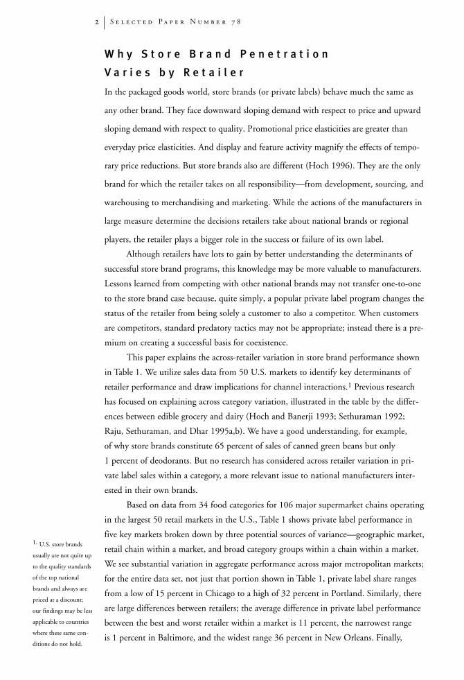
A b s t ra c t

Store brands are the only brand for which the retailer must

take on all responsibility—from development, sourcing,

and warehousing to merchandising and marketing.

Manufacturers’ actions largely drive the decisions retailers

take about national brands, but the retailer plays a more

determinant role in the success or failure of its own label.

Based on data from 34 food categories for 106 major su-

permarket chains operating in the largest 50 retail markets

in the U.S., we show that variation in store brand penetra-

tion across retailers is related systematically to underlying

consumer, retailer, and manufacturer factors. Store brand

market shares are influenced by trading area demographics;

retailer economies of scale and scope; retailer pricing, promotion, and assortment tactics; retailer

category expertise; local retail competition; within category brand competition; and manufacturer

promotion (push) and advertising strategies (pull) efforts. We argue that private label brands

threaten national brands most in categories when there is high variance in share across categories

(as opposed to high average share per se). In high variance categories, store brand share could in-

crease dramatically if the poor performing retailers imitate best practices.

Se l e c t e d Pa p e r 78

S e l e c t e d P a p e r N u m b e r 7 82

W h y S t o r e B r a n d P e n e t r a t i o n

V a r i e s b y R e t a i l e r

In the packaged goods world, store brands (or private labels) behave much the same as

any other brand. They face downward sloping demand with respect to price and upward

sloping demand with respect to quality. Promotional price elasticities are greater than

everyday price elasticities. And display and feature activity magnify the effects of tempo-

rary price reductions. But store brands also are different (Hoch 1996). They are the only

brand for which the retailer takes on all responsibility—from development, sourcing, and

warehousing to merchandising and marketing. While the actions of the manufacturers in

large measure determine the decisions retailers take about national brands or regional

players, the retailer plays a bigger role in the success or failure of its own label.

Although retailers have lots to gain by better understanding the determinants of

successful store brand programs, this knowledge may be more valuable to manufacturers.

Lessons learned from competing with other national brands may not transfer one-to-one

to the store brand case because, quite simply, a popular private label program changes the

status of the retailer from being solely a customer to also a competitor. When customers

are competitors, standard predatory tactics may not be appropriate; instead there is a pre-

mium on creating a successful basis for coexistence.

This paper explains the across-retailer variation in store brand performance shown

in Table 1. We utilize sales data from 50 U.S. markets to identify key determinants of

retailer performance and draw implications for channel interactions.1 Previous research

has focused on explaining across category variation, illustrated in the table by the differ-

ences between edible grocery and dairy (Hoch and Banerji 1993; Sethuraman 1992;

Raju, Sethuraman, and Dhar 1995a,b). We have a good understanding, for example,

of why store brands constitute 65 percent of sales of canned green beans but only

1 percent of deodorants. But no research has considered across retailer variation in pri-

vate label sales within a category, a more relevant issue to national manufacturers inter-

ested in their own brands.

Based on data from 34 food categories for 106 major supermarket chains operating

in the largest 50 retail markets in the U.S., Table 1 shows private label performance in

five key markets broken down by three potential sources of variance—geographic market,

retail chain within a market, and broad category groups within a chain within a market.

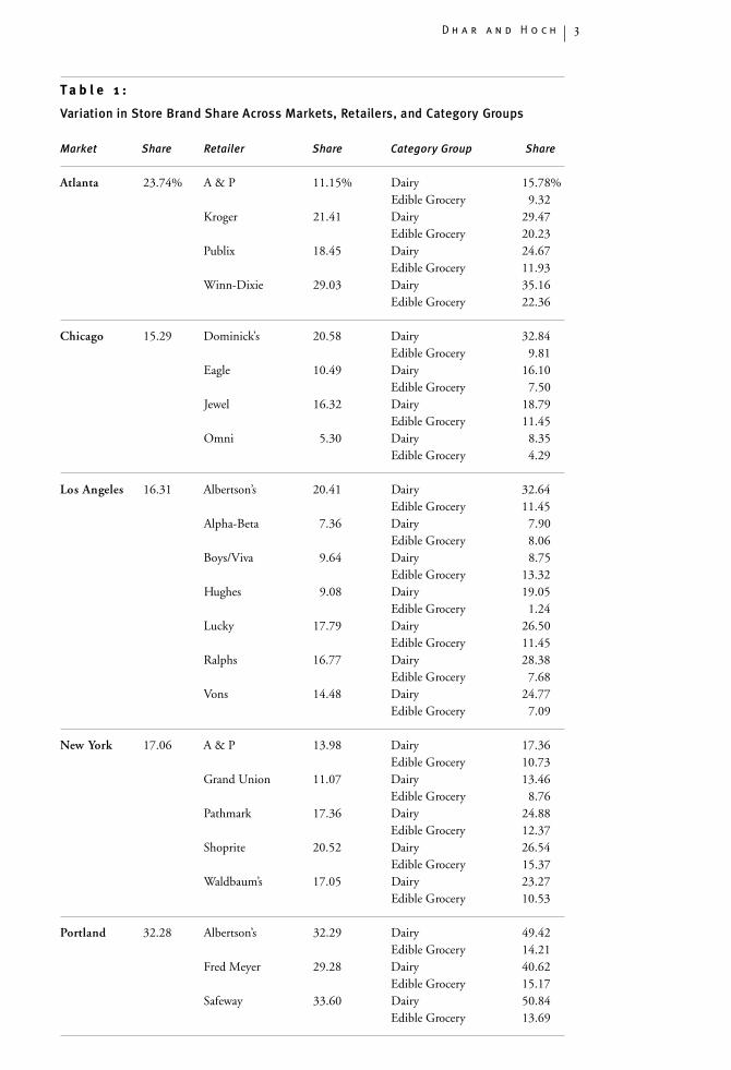
We see substantial variation in aggregate performance across major metropolitan markets;

for the entire data set, not just that portion shown in Table 1, private label share ranges

from a low of 15 percent in Chicago to a high of 32 percent in Portland. Similarly, there

are large differences between retailers; the average difference in private label performance

between the best and worst retailer within a market is 11 percent, the narrowest range

is 1 percent in Baltimore, and the widest range 36 percent in New Orleans. Finally,

1. U.S. store brands

usually are not quite up

to the quality standards

of the top national

brands and always are

priced at a discount;

our findings may be less

applicable to countries

where these same con-

ditions do not hold.

D h a r a n d H o c h 3

T a b l e 1 :

Variation in St o re Brand Share Across Markets, Retailers, and Category Gro u p s

M a r k e t S h a re Re t a i l e r S h a re C a t e g o ry Gro u p S h a re

At l a n t a 23.74% A & P 11.15% Dairy 15.78%Edible Grocery 9.32

Kroger 21.41 Dairy 29.47Edible Grocery 20.23

Publix 18.45 Dairy 24.67Edible Grocery 11.93

Winn-Dixie 29.03 Dairy 35.16Edible Grocery 22.36

C h i c a g o 15.29 Dominick’s 20.58 Dairy 32.84Edible Grocery 9.81

Eagle 10.49 Dairy 16.10Edible Grocery 7.50

Jewel 16.32 Dairy 18.79Edible Grocery 11.45

Omni 5.30 Dairy 8.35Edible Grocery 4.29

Los Angeles 16.31 Albertson’s 20.41 Dairy 32.64Edible Grocery 11.45

Alpha-Beta 7.36 Dairy 7.90Edible Grocery 8.06

Boys/Viva 9.64 Dairy 8.75Edible Grocery 13.32

Hughes 9.08 Dairy 19.05Edible Grocery 1.24

Lucky 17.79 Dairy 26.50Edible Grocery 11.45

Ralphs 16.77 Dairy 28.38Edible Grocery 7.68

Vons 14.48 Dairy 24.77Edible Grocery 7.09

New Yo rk 17.06 A & P 13.98 Dairy 17.36Edible Grocery 10.73

Grand Union 11.07 Dairy 13.46Edible Grocery 8.76

Pathmark 17.36 Dairy 24.88Edible Grocery 12.37

Shoprite 20.52 Dairy 26.54Edible Grocery 15.37

Waldbaum’s 17.05 Dairy 23.27Edible Grocery 10.53

Po rt l a n d 32.28 Albertson’s 32.29 Dairy 49.42Edible Grocery 14.21

Fred Meyer 29.28 Dairy 40.62Edible Grocery 15.17

Safeway 33.60 Dairy 50.84Edible Grocery 13.69

S e l e c t e d P a p e r N u m b e r 7 84

although there are stable differences at the retailer-market level, some retailers achieve

quite different levels of store brand performance depending on commodity type. For

instance, Omni has a weak program across the board while Winn-Dixie has a strong pro-

gram. On the other hand, Dominick’s is very strong in dairy but weak in edible grocery.

We carried out a more formal analysis of the complete data underlying Table 1:

private label market shares for each of three years broken down by the top 106 retailer/

market combinations in 34 food categories (3x34x106=10,812 observations). We esti-

mated a series of hierarchical models by regressing store brand market share onto subsets

of intercept terms representing categories, markets, retailers, and retailer x market inter-

actions. The results appear in Table 2.

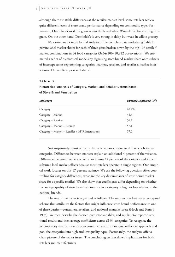
T a b l e 2 :

H i e ra rchical Analysis of Category, Market, and Retailer Determinants

of St o re Brand Pe n e t ra t i o n

I n t e rc e p t s Variance Explained (R2)

Category 40.2%

Category + Market 44.3

Category + Retailer 56.7

Category + Market + Retailer 57.1

Category + Market + Retailer + M*R Interactions 57.2

Not surprisingly, most of the explainable variance is due to differences between

categories. Differences between markets explain an additional 4 percent of the variance.

Differences between retailers account for almost 17 percent of the variance and in fact

subsume local market effects because most retailers operate in single regions. Our empiri-

cal work focuses on this 17 percent variance. We ask the following question: After con-

trolling for category differences, what are the key determinants of store brand market

share for a specific retailer? We also show that coefficients differ depending on whether

the average quality of store brand alternatives in a category is high or low relative to the

national brands.

The rest of the paper is organized as follows. The next section lays out a conceptual

scheme that attributes the factors that might influence store brand performance to one

of three parties—consumers, retailers, and national manufacturers (Hoch and Banerji

1993). We then describe the dataset, predictor variables, and results. We report direc-

tional results and then average coefficients across all 34 categories. To recognize the

heterogeneity that exists across categories, we utilize a random coefficient approach and

pool the categories into high and low quality types. Fortunately, the analyses offer a

clean picture of the major issues. The concluding section draws implications for both

retailers and manufacturers.

D h a r a n d H o c h 5

B a c k g r o u n d

We would prefer that a parsimonious theory could explain the across-retailer variation in Table 1,

but previous cross-category research suggests that this is unlikely (Hoch and Banerji 1993; Raju

et al. 1995a). The story is more complicated because store brands sit right in the middle of the

manufacturer-retailer-consumer vertical relationship. Unlike the typical national brand, where

consumer demand results from response to the pull

tactics of the manufacturer, U.S. store brands are the prototypical push product. If the retailer

decides to push the product, consumers will be exposed and respond accordingly depending on

underlying quality and other retailer actions, as well as whatever actions national manufacturers

coincidentally pursue.

Following Hoch and Banerji (1993), we localize the drivers of store brand performance

with the three parties that make up the retail channel: consumers, retailers, and manufacturers.

In a cross-sectional analysis of 185 grocery categories, Hoch and Banerji found that six variables

could explain 70 percent of the variance in market shares.

Store brands obtained higher market share when:

• quality relative to the national brands was high,

• quality variability of store brands was low,

• the product category was large in absolute terms ($ sales),

• percent gross margins were high,

• there were fewer national manufacturers operating in the category,

• national advertising expenditures were low.

The first two variables show that, all else equal, consumers are more likely to buy private labels

that provide parity quality. The middle two factors reflect the retailer’s scarce

resource allocation problem. Because retailers must draw on internal funds for the branding,

packaging, production, and advertising of their store brands, they invest more heavily in large

categories offering high profit margins so as to maximize their return. The last two variables

demonstrate the influence of manufacturers and show that private labels can be crowded out of

the market when national brand competition is high and when those brands invest advertising

resources into the consumer franchise. The differences

between dairy and edible grocery in Table 1 are consistent with this story—dairy has high quality

store brands (regulated by the USDA), huge sales volume and big margins, and few national

brands who spend little on advertising.

Determinants of performance in a cross-category analysis, however, are not necessarily the

ones that explain performance across retailers within a category. For example, quality, size of the

market, and gross margins vary more across categories than across

retailers within a category. Alternatively, demographic characteristics, level of promotion, and

pricing policy vary more across retailers than across categories. Conceptually, however, it is possi-

ble to localize the responsibility with the consumer, the retailer, or the manufacturer—and so we

will organize our discussion of the drivers of store brand penetration in this manner.

S e l e c t e d P a p e r N u m b e r 7 86

C o n s u m e r F a c t o r s

In order for consumers to influence retailer specific store brand performance, not only

must demographics matter but also differ by retailer. For economists, the typical store

brand sold in the U.S. is an inferior good and as such should be purchased more fre-

quently by price sensitive shoppers. Becker (1965) argues that systematic differences in

price sensitivity should emerge due to differences in opportunity costs of time associated

with demographic characteristics (Blattberg, Eppen, and Lieberman 1978). Starzynski

(1993) found that heavy private label users had lower incomes and larger blue collar

households with part time female heads of household. In a study of micromarket differ-

ences in demand for private labels, Hoch (1996) found that stores with larger category

price elasticities had higher private label share; moreover, there were systematic differ-

ences due to the demographic characteristics of a store’s trading area. Store brands ob-

tained higher share when the trading area contained more elderly people, lower housing

values and lower incomes, more large families, more working women, and higher educa-

tion levels. Each of these demographic relations is consistent with Becker’s opportunity

cost story except education.

Even though store-level sales of private label can be linked to consumer character-

istics, it is an empirical question whether these distinctions emerge when aggregating up

to the chain level. Do supermarket chains serve and attract sufficiently distinct clienteles?

Demographics could vary across retailers because of differences in targeting, positioning,

and real estate. Our data reveal wide disparities in demography by geographic region.

Compared to Los Angeles, Philadelphia has a larger elderly population (23 percent vs

17 percent) and significantly lower housing values (19 percent vs 41 percent of homes

worth more than $250,000). Demographic profiles also vary by retailer within a market.

In New Orleans, A&P serves a better educated clientele than Winn Dixie (21 percent

vs 16 percent college educated), while Schwegmann’s trading area contains more blacks

and hispanics (37 percent) than Delchamps (23 percent).

R e t a i l e r F a c t o r s

There are a large number of retailer characteristics that position some supermarket

chains to better develop and exploit a store brand program than others. First, we discuss

those factors largely fixed across categories and then address those that vary from category

to category.

Retail Competition. Retailers face different levels of competition depending on:

(a) the number of retail competitors; and (b) the heterogeneity in their market shares.

More competitors and a uniform distribution of shares leads to greater competition

(Waterson 1984). Facing a large set of competitors increases uncertainty; witness

Los Angeles retailers who must think about the potential actions of ten other major play-

ers versus Chicago where Jewel (35 percent share) is the long term price setter and

Dominick’s (21 percent) the price follower. Retailers operating in markets with lots

of competitors have smaller market shares on average and must focus on stealing

D h a r a n d H o c h 7

customers and defending their own turf. Retailers could use their store brand program to

help in this effort, but more likely will leverage national brand resources to build store

traffic. In contrast, with few competitors retailers have larger shares on average and plenty

to gain by exploiting existing store traffic, an objective that private label is particularly

well suited to achieve because of higher margins. Heterogeneity in market shares moder-

ates the effect of a fixed number of competitors; when a few chains dominate a market,

the retailer can safely focus attention on the major players and not worry about the

minor competitors. In the highly concentrated European food retailing scene, retailers

use store brands to differentiate themselves from the few big competitors they face.

Economies of Scale and Scope. Large retailers are better positioned to build scale

economies than smaller chains. Higher sales volumes bring down unit costs through:

(a) lower printing and holding costs for package labels; (b) better prices from suppliers

due to longer production runs and negotiating clout; and (c) lower inventory holding

costs through more continuous supply. These scale economies allow the retailer to pro-

vide better value for the money.

Retailers achieve economies of scope when corporate brand programs extend across

more of the 350 categories that full-service supermarkets typically carry. Presence in more

categories increases salience of the store brand concept and justifies investment in re-

sources dedicated to private label, such as in-house quality assurance, unique promotion

events, and a premium store brand program (e.g., Safeway Select). Retailers also signal

commitment through naming of the store brand—placing the chain name prominently

on 1,000-plus items makes the relation to the parent firm transparent. This reduces

consumer risk in trying products with unknown manufacturing origins and increases

motivation of employees responsible for merchandising the product. These scope factors

serve as surrogates for retailer effort and commitment to a store brand program.

EDLP and Breadth of Assortment. Consider the effect of EDLP (everyday low

pricing) versus Hi-Lo pricing on store brand performance (Hoch, Drèze and Purk 1994).

With less promotion activity and simpler merchandising tactics, EDLP makes the normal

price difference between the national brands and private label more apparent and facili-

tates parity comparisons. EDLP’s value orientation also is consistent with typical store

brand positioning. Depth of assortment also influences private label performance.

Retailers committed to a full service look offer more variety and deeper assortments, in-

cluding more slow moving items as they sacrifice efficiency for satisfying customer needs.

Narrow assortments favor the store brand; specialty items are more likely to be elimi-

nated, not private labels positioned against the leading national brands, sizes, and flavors.

C a t e g o ry Ex p e rtise. Retailers may develop special expertise in particular categories.

Some retailers excel in their presentation of meat and produce, while others have exper-

tise in better serving the eating needs of particular ethnic groups. Category expertise

develops in response to the demand side, but once developed, it becomes part of the

organization’s intellectual capital. The expert retail buyer is less dependent on national

S e l e c t e d P a p e r N u m b e r 7 88

brands to provide category knowledge and may use private labels to enhance margin mix

for an already high performance (in unit sales) category.

Price Gaps and Promotion. Category level pricing and promotion strategies could

influence store brand performance. The bigger the price gap between national brands and

private labels, the bigger is the incentive for the consumer to trade down to the private

label. Despite obvious economic arguments, evidence is mixed as to the importance of

relative price. In the cross category work of Raju et al. (1995b; Mills 1995; Sethuraman

1992), price differential actually is negatively related to private label performance—

categories with big gaps have lower private label penetration than those with smaller

gaps. Raju et al. (1995a) argue that this result is due to cross-sectional aggregation. In

equilibrium, differences in price sensitivity across categories lead to bigger gaps in price

insensitive categories (analgesics) and smaller gaps in price sensitive categories (canned

vegetables) where demand for private label is high. Hoch (1996) conducted single retailer

pricing experiments where the price gap varied from 10 to 35 percent. Private labels

were twice as sensitive to the gap as national brands, but price elasticities generally were

low, and so a profit maximizing retailer was better off with larger than smaller gaps. If

category price elasticities vary across retailers, however, different optimal price gaps

may emerge and within-category differences in price differentials may prove an impor-

tant predictor of store brand performance.

Just as the everyday pricing tactics of the retailer can influence private label perfor-

mance, so can the manner in which they promote products. Some markets and retailers

engage in aggressive week-to-week promotion battles; retailers use national brands as

loss leaders to build store traffic (Drèze 1995). Store brands lose their comparative advan-

tage when national brands are heavily promoted, especially amongst more price sensitive

buyers and heavy users who stockpile promoted product. Other retailers could elect to

aggressively promote private label—using shallow deals to help maintain a good margin

mix across products. But research on asymmetric cross-price elasticities between high

and low quality brands suggests that such tactics will be less effective for store brands

(Allenby and Rossi 1991) because they are more vulnerable to national brand promotion

and their own promotional efforts have less clout (Kamakura and Russell 1989).

Retailer Summary. All retailer factors are to some degree endogenous, even retail

competition and chain size. For econometric purposes, however, we assume that only

price gap, promotion, and assortment decisions are short term and endogenous enough

to require special treatment. Retailers can change chainwide policies (e.g., quality level)

but only in the long-run.

M a n u f a c t u r e r F a c t o r s

B rand Competition. National brands influence store brand performance directly with

various consumer pull tactics and indirectly through push tactics offered to the retail

channel. Probably the biggest influence on store brands is competition in the category.

As with retail competition, we follow the IO literature, which characterizes brand

D h a r a n d H o c h 9

competition as higher when: (a) there are a large number of national brands; and

(b) market shares are evenly distributed amongst the different brands (Waterson 1984).

When retailers carry many brands, there is a pure crowding out effect; on average, each

brand (including the store brand) will command a smaller share of a fixed pie (Raju et al.

1995b). Further, for a fixed number of national brands, higher concentration in market

shares among a few brands indicates less heterogeneity in tastes and possibly a price um-

brella, both conditions that are attractive to the store brand. When competing against a

couple of large share brands that may benefit from a price umbrella, store brands can

pursue a focused positioning strategy and offer an attractive alternative at a lower, but

still quite profitable, price. Alternatively, a store brand facing numerous same-size com-

petitive brands requires diffuse marketing effort in response to multiple fronts. Greater

brand competition hurts the store brand. Clearly the retailer has the final say over how

many brands they carry; we deal with this endogeneity in our econometrics.

Pull Promotion. A highly fragmented category is more sustainable for a national

brand than a private label because national brands benefit from the substantial economies

of scale in production and advertising that accrue to national distribution (Schmalensee

1978). Consider the RTE (ready-to-eat) cereal category, where about 200 brands are alive

at any point in time and 120 of them are actively marketed. Only a handful of brands

obtain more than 1 percent of the market and a majority have less than .5 percent. But

.5 percent of an $8 billion market is still an economically viable $40 million brand. The

problem for the store brand in a differentiated category is that the only way for the re-

tailer to grab significant share is to enter with multiple brands in disparate locations in

the product space, a practice that is self-limited by insufficient scale economies. In the

long run most manufacturer pull tactics serve to increase differentiation, reduce price

sensitivity, and increase top-of-mind awareness, each of which increase demand for na-

tional brands and hurt store brands. To the extent that advertising (TV, newsprint, and

magazine) and consumer promotion (coupons, sweepstakes, etc.) differ by markets, pull

promotion spending should limit store brand penetration.

Push Promotion. Trade promotion activity varies dramatically by geographic

market. Although manufacturers legally must offer identical terms of trade to resellers

competing in the same market, national brands can and do allocate trade dollars dispro-

portionately across markets depending on category development (consumption rate);

brand development (market share); and presence or absence of regional competition.

Trade promotion dollars take many forms but eventually are expressed at retail as reduc-

tions in everyday prices, temporary price reductions, or feature advertising and display.

Because manufacturers cannot directly set prices, these decisions are partly endogenous to

the retailer. At the same time, higher levels of trade spending do result in lower prices,

and manufacturers can contractually mandate performance requirements for feature

advertising and display. Greater levels of national brand promotion should limit private

label performance (Lal 1990).

S e l e c t e d P a p e r N u m b e r 7 810

S u m m a r y

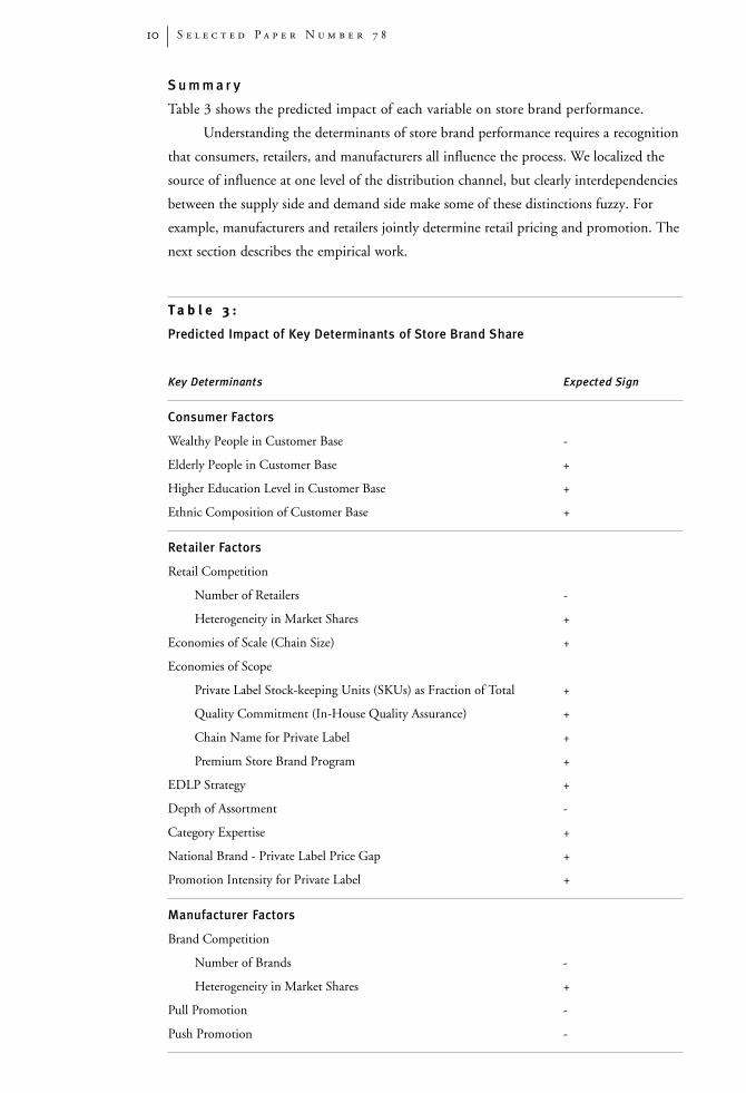
Table 3 shows the predicted impact of each variable on store brand perf o r m a n c e .

Understanding the determinants of store brand performance requires a recognition

that consumers, retailers, and manufacturers all influence the process. We localized the

source of influence at one level of the distribution channel, but clearly interdependencies

between the supply side and demand side make some of these distinctions fuzzy. For

example, manufacturers and retailers jointly determine retail pricing and promotion. The

next section describes the empirical work.

T a b l e 3 :

Predicted Impact of Key Determinants of St o re Brand Share

Key Determinants Expected Sign

Consumer Fa c t o r s

Wealthy People in Customer Base -

Elderly People in Customer Base +

Higher Education Level in Customer Base +

Ethnic Composition of Customer Base +

Retailer Fa c t o r s

Retail Competition

Number of Retailers -

Heterogeneity in Market Shares +

Economies of Scale (Chain Size) +

Economies of Scope

Private Label Stock-keeping Units (SKUs) as Fraction of Total +

Quality Commitment (In-House Quality Assurance) +

Chain Name for Private Label +

Premium Store Brand Program +

EDLP Strategy +

Depth of Assortment -

Category Expertise +

National Brand - Private Label Price Gap +

Promotion Intensity for Private Label +

M a n u f a c t u rer Fa c t o r s

Brand Competition

Number of Brands -

Heterogeneity in Market Shares +

Pull Promotion -

Push Promotion -

D h a r a n d H o c h 11

T h e S t u d y

We utilized four different data sources. A large packaged goods firm provided us with

the main database—syndicated sales data from A. C. Nielsen for all of their major prod-

uct categories and key retail accounts. Before reporting the results we present a detailed

description of the data sources and measures developed. We estimate individual category

regressions and then use a random coefficient approach to pool categories into two

quality types. Both analyses produce convergent findings about what drives variation

in store brand performance across retailers.

D a t a S o u r c e s

1. We use account data for 106 major U.S. grocery retail chains in the 50 Nielsen

SCANTRACK markets.2 This includes all retailers with average annual store sales of $2

million plus. These retail chains account for 60 percent of total supermarket sales in

the markets they serve. For each retail account, the dataset includes monthly brand level

information for 34 categories over three calendar years. The categories represent a wide

range of both edible grocery and dairy products including major categories such as

RTE cereal, coffee, and cheese and more minor ones like rice, marshmallows, and mus-

tard. Nielsen brand totals are used, aggregating all sizes and forms of each brand name.

Separate brand totals are reported for each distinct variant; for example, in cereal

Kellogg’s Corn Flakes and Kellogg’s Raisin Bran are reported as separate brands. Due to

confidentiality agreements all private label variants are aggregated into one brand total

even in cases where the retailer carries more than one label (e.g., President’s Choice).

The data provide detailed brand level information on both total equivalent unit

sales and dollar sales that is further subdivided into different components. Separate

subtotals are reported for sales accompanied with different forms of retail promotion

including the use of feature advertising, display, and temporary price reductions. Print

media expenditures (newspapers and magazines) are reported for all 50 markets but

TV advertising for only 23 major metropolitan markets. The database also includes

information on brand level consumer promotion offers.

2. We obtained detailed annual demographic data for each retailer from a syndi-

cated data service that overlay the trading area of each store onto the underlying census

tracts. This provided distributional information on age, income, ethnicity, education,

and home value.

3. Two published secondary data sources provide additional information on charac-

teristics of the retail chains and the markets served. For each SCANTRACK market,

Market Scope and Marketing Guidebook report each retailer’s (chains and independents)

overall market share, the number of stores operated, the average floor area, and the names

of the store brand lines carried to determine whether the chain uses its own name or

carries a premium store brand line. Both publications are well-known sources published

annually by Trade Dimensions, a unit of the Progressive Grocer Data Center.

2. Each SCANTRACK

area covers a designated

number of countries,

with an average of 30

and a range from 1 to

68. All markets include

central city, suburban,

and rural areas.

S e l e c t e d P a p e r N u m b e r 7 812

4. We also surveyed each of the retail accounts in the database. Retailers were asked

for information on their private label strategy, specifically for each of the three years:

(a) an estimate of the total number of private label SKUs and the number of categories

where they carried a private label; (b) whether or not they had a quality assurance pro-

gram for their private labels; and (c) names of key private label lines they carried.

Retailers also provided us with information on whether they followed an EDLP or Hi-Lo

pricing strategy. Multiple calls were made to the retail accounts leading to 93 of the 106

retailers completing the questionnaire.

M e a s u r e s U s e d i n t h e A n a l y s i s

We developed all measures at the retailer-market level. This means that Winn-Dixie in

Tampa is treated as a separate entity from Winn-Dixie in Dallas. We created yearly aggre-

gates for each measure resulting in three data points per retailer per category. We do so

for purposes of stability and the fact that about half of our measures are only available at

the annual level. This allows us to use the time series nature of our data to address certain

endogeneity issues.

Pr i vate Label Share (PL SH ARE). To normalize for differences in package size and

facilitate comparisons across categories, the dependent measure is the equivalent unit

(pounds) share of private labels (normal and premium variants) in a category for a retail

market account. Share is calculated as the ratio of total pound sales for the private label

to total pound sales for the whole category. For exposition, share is expressed in percent-

age terms. Using dollar sales instead of equivalent unit sales or a logit transformation of

these market shares led to similar insights.

Home Value (HOME VAL). This variable measures the extent to which the customer

base for a retail account is comprised of wealthier individuals. HOMEVAL measures the

fraction of total number of households for a retail account owning homes with value

higher than $250,000; it is highly correlated (r=.79) with income (percent greater than

$50,000). We expect a negative coefficient because wealthier consumers are less price sen-

sitive due to higher opportunity costs.

Elderly (EL D ER LY). This variable is operationalized as the fraction of a retailer’s

customer base that is older than 55 years. Because the elderly have lower opportunity

costs and more severe budget constraints, the coefficient should be positive.

Education (EDUC). This variable is given by the fraction of households in a retail

account’s customer base with a four-year college degree. Despite obvious income effects,

we predict a positive coefficient (Hoch 1996). If educated consumers have greater shop-

ping expertise, they may rely less on brand name as an indicator of product performance.

Ethnic (ET HNIC). The extent to which a retail account serves minority groups is

measured by the fraction of black and hispanic households. Although conventional in-

dustry wisdom suggests that blacks and hispanics are more likely to buy well known

brand names, we predict a positive coefficient as found by Hoch (1996).

D h a r a n d H o c h 13

Retail Competition (#RETA IL, RETVAR). Two measures capture the extent of retail

competition in a local market: the number of retail competitors (#RETAIL) and the het-

erogeneity in shares across these retailers (RETVAR). #RETAIL is directly measured from

Market Scope. Heterogeneity is captured as the variance (s2) in market shares. Retail

competition is higher with lots of competitors and is lower when heterogeneity in shares

is greater, implying a negative coefficient for #RETAIL and a positive one for RETVAR.

Chain Size (SI ZE). Size of the chain is captured by the number of stores that each

retailer operates in a particular market. Conceptually, it represents the potential for a re-

tailer to benefit from economies of scale and should be positively related to private label

share. Using total square footage of the chain (number of stores times average square

footage) produced similar results.

Pr i vate Label SKUs (PL SKU). This variable is the total number of private label

sku’s expressed as a fraction of the total number of SKUs across all categories in the store

and represents the potential for economies of scope. As with SIZE, the coefficient should

be positive.

Quality Assurance for Pr i vate Labels (QUAL). This is an indicator variable, where

QUAL=1 if the retail account has a quality program and QUAL=0 otherwise. This

variable represents a signal about the retailer’s commitment to private label quality and

to some extent may capture actual quality differences across retailers. The coefficient

should be positive.

Own Name Label (PL NAME). Using information on private label names provided

in the Marketing Guidebook and cross verifying through the survey, we create an indicator

variable PLNAME=1 when the chain uses its own label and 0 otherwise. It should have

a positive sign.

EDLP / H i - Lo Pricing St rategy (EDLP). EDLP=1 when chains use an everyday low

pricing strategy and 0 when they go Hi-Lo. Retailers initially were classified based on

their answers to the survey, and corroborated through a search of trade press. The regular

price gap between national and store brands was 36 percent in EDLP chains vs 44 per-

cent in Hi-Lo chains. EDLP chains also sold less product on deal, 20 percent of private

label and 25 percent of national brands compared to 24 percent and 30 percent respec-

tively in Hi-Lo chains. We expect EDLP to have a positive sign.

Premium Label (PREMIUM). Using information from the manufacture r’s sales forc e ,

the retailer surve y, and published secondary sources, we determined that PREMIUM=1

when a retailer stocks a higher quality and premium price label (e.g., President’s Choice)

in addition to their normal store brands. We would prefer to examine premium private

labels separately but confidentiality agreements require Nielsen to aggregate across store

brand types when providing syndicated data to manufacturers. The premium variable

probably captures both the effect of a larger number and likely greater differentiation

of store brands in any one category (normal plus premium) and may serve as a surrogate

for retailer commitment to the whole idea of a store brand program. The expected

sign is positive.

S e l e c t e d P a p e r N u m b e r 7 814

Depth of Assortment (AVG SKU). The extent of category-specific item proliferation is

measured by the average number of stock-keeping units (SKUs) carried in that category av-

eraged across stores in a particular retail chain. This measure was created from

another database providing more detailed item level information. Because we account

for the number of national brands separately, this variable measures the level of variety that

the retailer offers for the average national brand. We endogenize this variable because the re-

tailer has final say. AVGSKU should have a negative sign.

C a t e g o ry Development Index (CDI). The CDI for a retail account is an index

measuring the account’s category share of total equivalent unit sales volume in a market rela-

tive to its total size (measured by all commodity volume, or ACV$) in the market.

By normalizing for the relative size of the retail account, the measure captures the extent to

which the retailer does well in a specific category relative to performance across all

categories. This is given by,

Account Eqvt. Unit Volume for Category Market ACV$CDI = x

Market Eqvt. Unit Volume for Category Account ACV$

Normalizing retailer volume by the total U.S. leads to the same results. Categories

with a high CDI are relatively more important to that retailer and therefore likely to draw

more attention. We view CDI as a long-run surrogate for category expertise, though we rec-

ognize the likely recursive relationship between expertise and the demand side. Although we

are unaware of any studies showing that heavy category users buy

a disproportionate amount of private label, this could lead to a contemporaneous correlation

between CDI and private label share, and so we endogenize the variable. The

CDI coefficient should be positive.

National Bra n d - Pr i vate Label Price Differential (PRD IFF). The price gap is measured

as the price difference per equivalent unit between the average national brand and the pri-

vate label divided by the average national brand price. We compute both the shelf price dif-

ferential and the regular price differential using information on total and nonpromoted

sales, respectively. Sales (in equivalent units) weighted as well as unweighted average brand

prices were computed. Since alternate measures—weighted or unweighted, shelf or regular

price differentials—led to the same insights, we report results only for the u n weighted re g u-

lar price differential measure. Larger price gaps should lead to better store brand perfor-

mance. Since national brand and private label cross-price effects can influence the setting of

the price differential and store brand share, we endogenize this va r i a b l e .

Pe rcentage Pr i vate Label Volume Sold on Deal (PLP ROMO). This variable measures

the average retail promotion intensity for the store brand and is given by the

fraction of total equivalent unit volume sold when accompanied by any kind of retail pro-

motion including temporary price reductions, feature advertising, and display. Collinearity

precluded use of more detailed breakups. The coefficient should be positive.

Pe rcentage National Brand Volume Sold on Deal (NBP ROMO). Promotion intensity

of national brands is measured by the fraction of its total equivalent unit sales

D h a r a n d H o c h 15

volume sold with any kind of retail promotion. The coefficient should be negative.

Conceptually both PLPROMO and NBPROMO are equivalent to promotion elasticity

times frequency of promotion. For reasons cited for PRDIFF, we endogenize both

PLPROMO and NBPROMO.

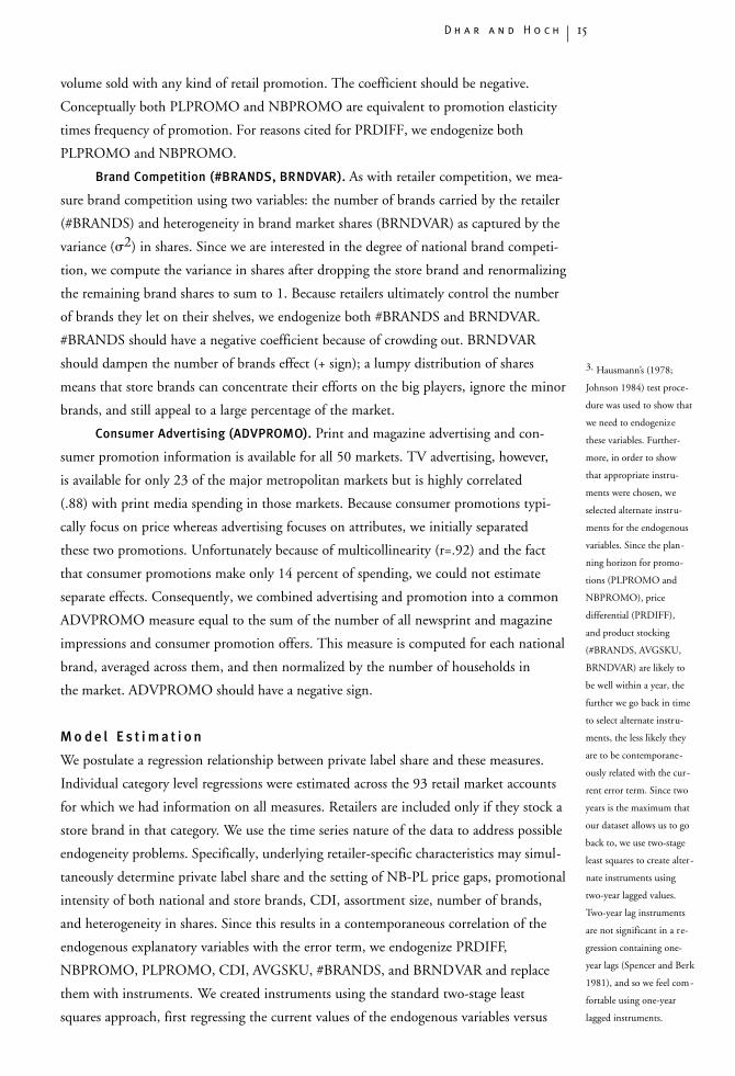
B rand Competition (#BR ANDS, BRNDVAR). As with retailer competition, we mea-

sure brand competition using two variables: the number of brands carried by the retailer

(#BRANDS) and heterogeneity in brand market shares (BRNDVAR) as captured by the

variance (s2) in shares. Since we are interested in the degree of national brand competi-

tion, we compute the variance in shares after dropping the store brand and renormalizing

the remaining brand shares to sum to 1. Because retailers ultimately control the number

of brands they let on their shelves, we endogenize both #BRANDS and BRNDVAR.

#BRANDS should have a negative coefficient because of crowding out. BRNDVAR

should dampen the number of brands effect (+ sign); a lumpy distribution of shares

means that store brands can concentrate their efforts on the big players, ignore the minor

brands, and still appeal to a large percentage of the market.

Consumer Adve rtising (ADV P ROMO). Print and magazine advertising and con-

sumer promotion information is available for all 50 markets. TV advertising, however,

is available for only 23 of the major metropolitan markets but is highly correlated

(.88) with print media spending in those markets. Because consumer promotions typi-

cally focus on price whereas advertising focuses on attributes, we initially separated

these two promotions. Unfortunately because of multicollinearity (r=.92) and the fact

that consumer promotions make only 14 percent of spending, we could not estimate

separate effects. Consequently, we combined advertising and promotion into a common

ADVPROMO measure equal to the sum of the number of all newsprint and magazine

impressions and consumer promotion offers. This measure is computed for each national

brand, averaged across them, and then normalized by the number of households in

the market. ADVPROMO should have a negative sign.

M o d e l E s t i m a t i o n

We postulate a regression relationship between private label share and these measures.

Individual category level regressions were estimated across the 93 retail market accounts

for which we had information on all measures. Retailers are included only if they stock a

store brand in that category. We use the time series nature of the data to address possible

endogeneity problems. Specifically, underlying retailer-specific characteristics may simul-

taneously determine private label share and the setting of NB-PL price gaps, promotional

intensity of both national and store brands, CDI, assortment size, number of brands,

and heterogeneity in shares. Since this results in a contemporaneous correlation of the

endogenous explanatory variables with the error term, we endogenize PRDIFF,

NBPROMO, PLPROMO, CDI, AVGSKU, #BRANDS, and BRNDVAR and replace

them with instruments. We created instruments using the standard two-stage least

squares approach, first regressing the current values of the endogenous variables versus

3. Hausmann’s (1978;

Johnson 1984) test proce-

dure was used to show that

we need to endogenize

these variables. Further-

more, in order to show

that appropriate instru-

ments were chosen, we

selected alternate instru-

ments for the endogenous

variables. Since the plan-

ning horizon for promo-

tions (PLPROMO and

NBPROMO), price

differential (PRDIFF),

and product stocking

(#BRANDS, AVGSKU,

BRNDVAR) are likely to

be well within a year, the

further we go back in time

to select alternate instru-

ments, the less likely they

are to be contemporane-

ously related with the cur-

rent error term. Since two

years is the maximum that

our dataset allows us to go

back to, we use two-stage

least squares to create alter-

nate instruments using

two-year lagged values.

Two-year lag instruments

are not significant in a re-

gression containing one-

year lags (Spencer and Berk

1981), and so we feel com-

fortable using one-year

lagged instruments.

S e l e c t e d P a p e r N u m b e r 7 816

the one-year lags and then using the predicted values.3 The instrumented variables do

not remain constant from year to year. We also checked for a first order autoregressive

process by assuming the same serial coefficient across retailers. We estimated the serial

correlation using the data for all retailers by regressing the estimated error for a year

against the preceding year’s estimated error. We lost one year of data due to the instru-

mented variables. Our analysis indicated no serial correlation in the data.4

For each category, we regress account level private label share against the corre-

sponding explanatory variables for a two year period since we lose the first year of data

when computing the instruments. Pooling tests show no differences in the value of the

estimated coefficients across the two years in any of the category regressions. Therefore,

we run individual category level regressions by pooling the data across the two years.

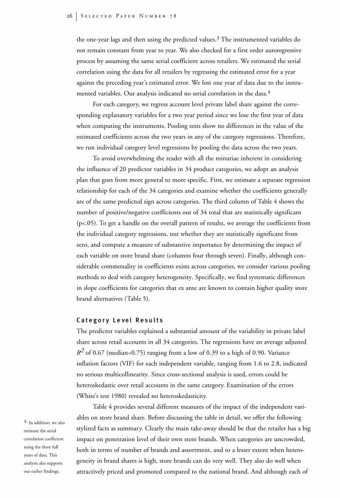
To avoid overwhelming the reader with all the minutiae inherent in considering

the influence of 20 predictor variables in 34 product categories, we adopt an analysis

plan that goes from more general to more specific. First, we estimate a separate regression

relationship for each of the 34 categories and examine whether the coefficients generally

are of the same predicted sign across categories. The third column of Table 4 shows the

number of positive/negative coefficients out of 34 total that are statistically significant

(p<.05). To get a handle on the overall pattern of results, we average the coefficients from

the individual category regressions, test whether they are statistically significant from

zero, and compute a measure of substantive importance by determining the impact of

each variable on store brand share (columns four through seven). Finally, although con-

siderable commonality in coefficients exists across categories, we consider various pooling

methods to deal with category heterogeneity. Specifically, we find systematic differences

in slope coefficients for categories that ex ante are known to contain higher quality store

brand alternatives (Table 5).

C a t e g o r y L e ve l R e s u l t s

The predictor variables explained a substantial amount of the variability in private label

share across retail accounts in all 34 categories. The regressions have an average adjusted

R2 of 0.67 (median=0.75) ranging from a low of 0.39 to a high of 0.90. Variance

inflation factors (VIF) for each independent variable, ranging from 1.6 to 2.8, indicated

no serious multicollinearity. Since cross-sectional analysis is used, errors could be

heteroskedastic over retail accounts in the same category. Examination of the errors

(White’s test 1980) revealed no heteroskedasticity.

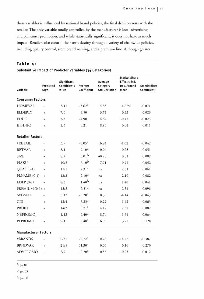
Table 4 provides several different measures of the impact of the independent vari-

ables on store brand share. Before discussing the table in detail, we offer the following

stylized facts as summary. Clearly the main take-away should be that the retailer has a big

impact on penetration level of their own store brands. When categories are uncrowded,

both in terms of number of brands and assortment, and to a lesser extent when hetero-

geneity in brand shares is high, store brands can do very well. They also do well when

attractively priced and promoted compared to the national brand. And although each of

4. In addition, we also

estimate the serial

correlation coefficient

using the three full

years of data. This

analysis also supports

our earlier findings.

D h a r a n d H o c h 17

T a b l e 4 :

S u b s t a n t i ve Impact of Predictor Variables (34 Categories)

Market Share

S i g n i f i c a n t Ave ra g e Effect 1 St d .

Pre d i c t e d C o e f f i c i e n t s Ave ra g e C a t e g o ry D e v. Around Standardized

Va r i a b l e S i g n # + / # - C o e f f i c i e n t Std Deviation M e a n C o e f f i c i e n t

Consumer Fa c t o r s

HOMEVAL - 3/11 -5.62a 14.83 -1.67% -0.071

ELDERLY + 7/0 4.50 3.72 0.33 0.023

EDUC + 5/5 -4.90 4.67 -0.45 -0.023

ETHNIC + 2/6 0.21 8.83 0.04 0.011

Retailer Fa c t o r s

#RETAIL - 3/7 -0.05a 16.24 -1.62 -0.042

RETVAR + 8/1 9.10a 0.04 0.73 0.051

SIZE + 8/2 0.01b 40.25 0.81 0.007

PLSKU + 10/2 6.10b 7.71 0.94 0.042

QUAL (0-1) + 11/1 2.31a na 2.31 0.061

PLNAME (0-1) + 12/2 2.10a na 2.10 0.082

EDLP (0-1) + 8/3 1.40b na 1.40 0.041

PREMIUM (0-1) + 13/2 2.51a na 2.51 0.096

AVGSKU - 5/12 -0.20a 10.36 -4.14 -0.043

CDI + 12/4 3.23a 0.22 1.42 0.063

PRDIFF + 14/2 8.21a 14.12 2.32 0.082

NBPROMO - 1/12 -9.40a 8.74 -1.64 -0.064

PLPROMO + 9/1 9.48a 16.98 3.22 0.128

M a n u f a c t u rer Fa c t o r s

#BRANDS - 0/31 -0.72a 10.26 -14.77 -0.387

BRNDVAR + 21/5 51.30a 0.06 6.16 0.270

ADVPROMO - 2/9 -0.20a 0.58 -0.23 -0.012

a: p<.01

b: p<.05

c: p<.10

these variables is influenced by national brand policies, the final decision rests with the

retailer. The only variable totally controlled by the manufacturer is local advertising

and consumer promotion, and while statistically significant, it does not have as much

impact. Retailers also control their own destiny through a variety of chainwide policies,

including quality control, store brand naming, and a premium line. Although greater

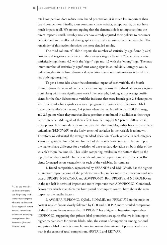
S e l e c t e d P a p e r N u m b e r 7 818

retail competition does reduce store brand penetration, it is much less important than

brand competition. Finally, most consumer characteristics, except wealth, do not have

much impact at all. We are not arguing that the demand side is unimportant but the

direct impact is small. Possibly retailers have already adjusted their policies to consumer

behavior and so the effect of demographics is partially subsumed in other variables. The

remainder of this section describes the more detailed results.

The third column of Table 4 reports the number of statistically significant (p<.05)

positive and negative coefficients. In the average category 8 out of 20 coefficients were

statistically significant, 6.5 with the “right” sign and 1.5 with the “wrong” sign. The max-

imum number of statistically significant wrong signs in an individual category was 3,

indicating deviations from theoretical expectations were not systematic or isolated to a

few outlying categories.

To get a better idea about the substantive impact of each variable, the fourth

column shows the value of each coefficient averaged across the individual category regres-

sions along with t-test significance levels.5 For example, looking at the average coeffi-

cients for the four dichotomous variables indicates that store brands gain 2.3 share points

when the retailer has a quality assurance program, 2.1 points when the private label

carries the retailer’s own name, 1.4 points when the retailer follows an EDLP strategy,

and 2.5 points when they merchandise a premium store brand in addition to their regu-

lar private label. Adding all of these effects together imply a 8.3 percent difference in

share points. It is more difficult to interpret the other variables, either because the scale is

unfamiliar (BRNDVAR) or the likely extent of variation in the variable is unknown.

Therefore, we calculated the average standard deviation of each variable in each category

across categories (column 5), and for each of the nondichotomous variables, we report

the market share difference for a variation of one standard deviation on both sides of the

variable’s mean (column 6). This is like comparing retailers in the bottom third to the

top third on that variable. In the seventh column, we report standardized beta coeffi-

cients (averaged across categories) for each of the variables. In summary:

1. Brand competition, represented by #BRANDS and BRNDVAR, has the highest

substantive impact among all the predictor variables, in fact more than the combined im-

pact of PRDIFF, NBPROMO, and ADVPROMO. Both PRDIFF and NBPROMO are

in the top half in terms of impact and more important than ADVPROMO. Combined,

factors over which manufacturers have partial or complete control have about the same

impact as the retailer factors.

2. AVGSKU, PLPROMO, QUAL, PLNAME, and PREMIUM are the most im-

portant retailer factors closely followed by CDI and EDLP. A more detailed comparison

of the different factors reveals that PLPROMO has a higher substantive impact than

NBPROMO, suggesting that private label promotions are quite effective in leading to

higher market share for private labels. Also, the extent of competition among national

and private label brands is a much more important determinant of private label share

than is the extent of retail competition, #RETAIL and RETVAR.

5. This also provides

an alternative estima-

tion for pooling coeffi-

cients across categories

when the random coef-

ficient approach cannot

be used, either due to

violation of underlying

assumptions or data

limitations (Bass and

Wittink 1978).

3. Finally, consumer factors have a much lower impact on private label share per-

formance than either the manufacturer or retailer factors; HOMEVAL is the only demo-

graphic variable having a substantial impact.

P o o l e d A n a l y s i s a c r o s s C a t e g o r i e s

It is unrealistic to expect that the slope coefficients are homogeneous across all 34 cate-

gories, and so in the next section we consider methods of pooling information across cat-

egories. This will not only help get precise estimates of the common pattern but also

better summarize central tendencies in the data. We specify the system of category regres-

sions as part of a multivariate regression system making the following error assumptions

and using the following notation:

msc=Xßc + ec; c=1, 2, . . .34.

We assume that e´=(e1, e2, . . . ec) , MVN (0, Λ^In); Λ = Diag (s21, . . . .,s2

c).

msc is the vector of private label shares for the cth category expressed in terms of devia-

tions from the mean category share across the retail accounts. X is the Nxk matrix of

values for the k independent variables, each variable being expressed in terms of devia-

tions from the within-category mean across retailer accounts. N is the number of retail

accounts. ßc is the cth category slope coefficient vector and ec is the Nx1 vector of error

terms for the c th category. Mean centering by category of both the dependent and inde-

pendent variables is equivalent to removing the main effect (category intercepts) of

category. Consequently, our pooled analysis seeks to explain the variation in private label

share across retail accounts as opposed to identifying factors that might explain differ-

ences in mean private label share across categories.

We also assume that (a) the error terms are independent across retail accounts

within a given category, i.e., ec,MVN(0, s2cIn); and (b) that the errors across

categories for the same retail account are independent. Our careful selection of the rele-

vant independent variables justifies the first assumption. The second assumption is

justified by an analysis of the correlation matrix of the errors across individual category

level regressions.

Formal testing of the pooling restriction assuming that the slope coefficients are the

same across the category regressions is rejected. This is not surprising given large differ-

ences in within-category variance in private label share between categories. Therefore,

we searched for a partitioning variable that satisfied two criteria: (a) it led to a substantial

reduction in within-group heterogeneity; and (b) it was theoretically justified so as to

facilitate interpretation of any differences in slope coefficients that might emerge. Past

research suggests that actual quality of the store brand is an important determinant of

store brand performance (Hoch and Banerji 1993). In categories offering lower quality

store brands, the price gap and demographic factors influencing consumer price sensitiv-

ity may be more influential in explaining retailer performance. In contrast, factors related

to the retailers’ reputation and ability to differentiate themselves from competition may

D h a r a n d H o c h 19

´ ´ ´

S e l e c t e d P a p e r N u m b e r 7 820

be more important in categories with higher quality store brands. To complete this analy-

sis, we took recent category quality estimates from Hoch and Banerji (1993). They

elicited category level estimates of store brand quality from 25 quality assurance managers

at leading U.S. supermarket chains and wholesalers. We utilized their rankings, rank-

ordered the 34 categories, and performed a median split into higher and lower quality

types. Although this ex ante quality measure is not perfect, it was the best available to us.

We use a random coefficient regression procedure in order to estimate the mean

coefficients for the two quality groups. Our procedure is similar to that used in the pool-

ing literature (Bass and Wittink 1975, 1978; Hoch, Kim, Montgomery, and Rossi 1995).

We assume that the category coefficient vectors for the high quality categories are draws

from a super-population distribution with mean ßh and variance Vßh. Similarly, the co-

efficient vectors for the low categories are draws from a super-population distribution

with mean ßl and variance Vßl. That is, within the high and low quality category groups,

the category coefficient vectors are distributed i.i.d. with means ßh and ßl and corre-

sponding variances of Vßh and Vßl. To characterize the central tendency or commonality

among the categories within each quality type, we would like to infer the means for each

of the quality types. Using the procedure in Hoch et al. (1995), we use the entire dataset

to obtain consistent estimates of the mean slope coefficient vector for the low quality cat-

egories and the differences in the mean slope coefficients between the two quality types.

This is used to compute the mean slope coefficient vector for the high quality categories.

Asymptotically justified estimates of the variance-covariance matrix are used to determine

the significance level of the two mean slope coefficient vectors.

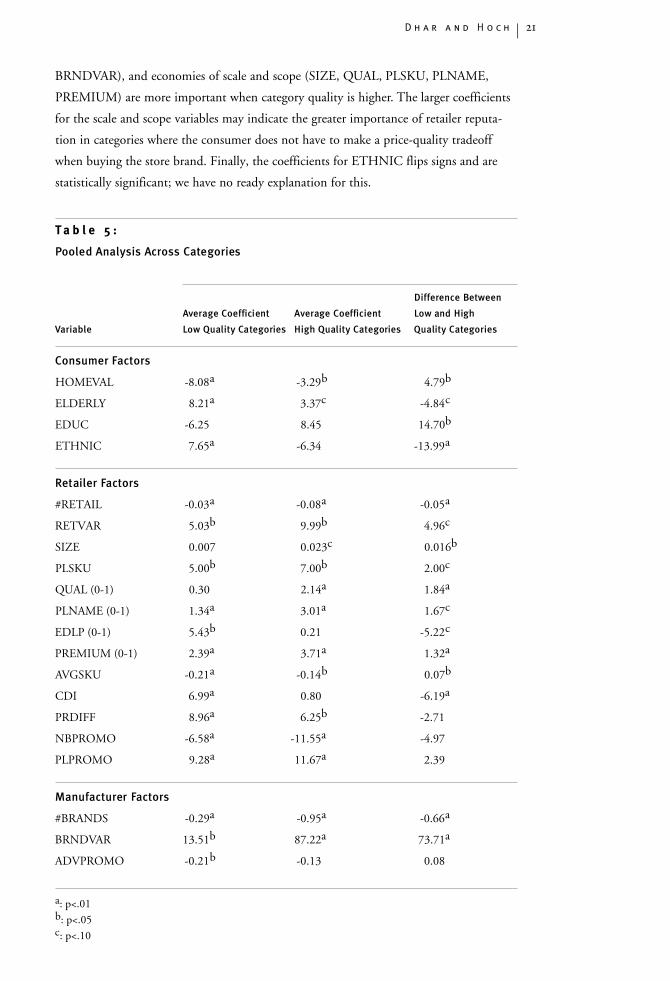
Table 5 presents the mean slope coefficient vector for the two quality types. We

also report the interaction terms testing the differences in the mean slope coefficients

between the high and low quality categories. The pooled analysis presents quite a clean

picture, one that generally reinforces the conclusions from the individual category regres-

sions. Only the EDUC variable is not statistically significant for either the high or low

quality groups or both. The 3.16 intercept difference between the two quality types indi-

cates that even after controlling for all the other variables, higher quality categories have

higher store brand penetration than lower quality categories. For 4 of the 20 predictor

variables, the slope coefficients do not differ by quality level: PRDIFF, NBPROMO,

PLPROMO, and ADVPROMO. Several of the variables have more impact (i.e., absolute

value) in the low quality categories. For example, the fact that low quality categories have

larger coefficients (in absolute value) for HOMEVAL, ELDERLY, and EDLP suggests

that price and consumers’ reaction to it are more important when store brand quality is

not up to the standards of the national brands, that is when the store brand truly is an

inferior good in the economic sense. CDI also is more important in lower quality cate-

gories, a finding that might indicate that category expertise is more important when it is

difficult to offer a top-quality store brand.

The remaining coefficients have larger slopes in the high quality categories. Degree

of competition, at both the brand and retail level (#RETAIL, RETVAR, #BRANDS,

D h a r a n d H o c h 21

BRNDVAR), and economies of scale and scope (SIZE, QUAL, PLSKU, PLNAME,

PREMIUM) are more important when category quality is higher. The larger coefficients

for the scale and scope variables may indicate the greater importance of retailer reputa-

tion in categories where the consumer does not have to make a price-quality tradeoff

when buying the store brand. Finally, the coefficients for ETHNIC flips signs and are

statistically significant; we have no ready explanation for this.

T a b l e 5 :

Pooled Analysis Across Categories

D i f f e rence Betwe e n

Ave rage Coefficient Ave rage Coefficient Low and High

Va r i a b l e Low Quality Categories High Quality Categories Quality Categories

Consumer Fa c t o r s

HOMEVAL -8.08a -3.29b 4.79b

ELDERLY 8.21a 3.37c -4.84c

EDUC -6.25 8.45 14.70b

ETHNIC 7.65a -6.34 -13.99a

Retailer Fa c t o r s

#RETAIL -0.03a -0.08a -0.05a

RETVAR 5.03b 9.99b 4.96c

SIZE 0.007 0.023c 0.016b

PLSKU 5.00b 7.00b 2.00c

QUAL (0-1) 0.30 2.14a 1.84a

PLNAME (0-1) 1.34a 3.01a 1.67c

EDLP (0-1) 5.43b 0.21 -5.22c

PREMIUM (0-1) 2.39a 3.71a 1.32a

AVGSKU -0.21a -0.14b 0.07b

CDI 6.99a 0.80 -6.19a

PRDIFF 8.96a 6.25b -2.71

NBPROMO -6.58a -11.55a -4.97

PLPROMO 9.28a 11.67a 2.39

M a n u f a c t u rer Fa c t o r s

#BRANDS -0.29a -0.95a -0.66a

BRNDVAR 13.51b 87.22a 73.71a

ADVPROMO -0.21b -0.13 0.08

a: p<.01 b: p<.05 c: p<.10

S e l e c t e d P a p e r N u m b e r 7 822

C o n c l u s i o n s

This study shows how and why the performance of private label programs systematically

vary across retailers. Although our analysis shows that the pull and push tactics of the na-

tional brands exert an important influence on store brand performance, we find that a

substantial part of the variation in market share comes about from actions taken by the

retailer, either independently as part of their overall marketing strategy or in response to

manufacturer actions. Key insights are as follows:

1. Overall chain strategy in the use of EDLP pricing, commitment to quality,

breadth of private label offerings, use of own name for private label, a premium store

brand offering, and number of stores consistently enhance the retailer’s private label share

performance in all categories. Also, the extent to which the retailer serves a customer base

containing less wealthy and more elderly households and operates in less competitive

markets improves the performance of the store brand.

2. Although an EDLP positioning (and the concomitant lower level of national

brand promotion) helps the store brand, there are countervailing effects. A lower price

gap and less private label promotion accompanying EDLP work in the opposite direc-

tion. Furthermore, the EDLP positioning benefits the store brand only in lower quality

categories where the value positioning of the store may be better aligned with the price

advantage of the store brand. Our regression models suggest, however, that the net result

is quite positive for the average EDPL store. By plugging in the average values for all the

other variables into the equations, we find that the average predicted EDPL store cap-

tures 3.8 more store brand share points when compared to the average Hi-Lo competitor.

3. Recent statements in the popular press document an increased use of merchan-

dising activities by retailers. Our analysis suggests that retailer promotional support can

significantly enhance private label share performance.

4. Retailers often use national brands to draw customers to their stores. Retailers

who pursue this traffic building strategy usually carry more national brands and broader

assortments and offer better everyday (lower price gap) and promotional prices on na-

tional brands. Each of these actions work against the retailer’s own store brands, high-

lighting the important balancing act the retailer must perform to profitably manage the

sales revenue and margin mix in each of their categories. At the same time, adding a

higher quality premium store brand program may mitigate this trade-off.

5. Unlike cross-category studies, our within-category across-retailer analysis shows

that the national brand-private label price differential exerts an important positive influ-

ence on store brand performance. Across all categories, the average gap is about 40 per-

cent (range 20 to 60 percent). Our data show that a 10 percent change in the price gap

fraction results in a 0.8 percent change in store brand share (average ß=8.2). This sup-

ports the contention that the negative sign for price gap observed in previous research

probably results from cross-category aggregation problems (Raju et al. 1995b).6

6. A cross-category

analysis for the current

dataset also leads to a

similar result for the

price gap.

D h a r a n d H o c h 23

6. When retailers obtain more than their fair share of a category (high CDI),

they also do much better with private label. On average a retailer performing 10 percent

better than the norm (CDI=110 vs 100) will have a store brand with 3 percent higher

market share.

7. From the national brand’s perspective, encouraging the retailer to carry more

brands (#BRANDS) and deeper assortments (AVGSKU) may be the most effective ways

to keep store brands in check. And although an even distribution of brands also works

against the store brand, it is unclear how manufacturers can influence BRNDVAR.

The importance of these variables, however, may depend on the national brand’s market

position. For example, a category leader may be glad to see a rise in store brand share

if it comes at the expense of one of its secondary national brand competitors. For in-

stance, although P&G’s efforts to streamline assortment appear aimed at creating market-

ing and operating efficiencies, the end result may be an increase in store brand sales at

the expense of minor brands. Low share underdogs are extremely vulnerable to assort-

ment reductions.

8. The exact impact of most of the variables depends on the underlying quality

of store brands in a category. When store brand quality is high, competition at the retail

and brand level is more important, as are variables capturing economies of scale and

scope enjoyed by the retailer. In contrast, demographics associated with consumer price

sensitivity and EDPL pricing matter more in low quality categories.

9. Finally, premium store brands may offer the retailer an avenue for responding

to the national brand’s ability to cater to heterogeneous preferences. This appears more

likely in categories where store brands already offer high quality comparable to the

national brands.

Appreciating what separates the best from the worst retailers is important for both

retailers and manufacturers. Although understanding “best practices” is generically im-

portant no matter the industry, we would argue that it is even more important in retail-

ing. The reason is that retailers can easily observe each others actions, assess the impact

of those actions, and quickly imitate successful strategies. For retailers, arguably the most

important practices are those that successfully build store traffic (e.g., new store formats,

store appearance, perimeter departments, advertising) and produce significant shifts in

market share.7 Leading manufacturers must be alert to these changing practices, but

in general will get their fair share of category sales irrespective of which retailer makes the

sale. On the other hand, retailer imitation of successful store brand programs is more

threatening to national manufacturers because within-store loss of share to the retailer’s

store brand (or for that matter to another national brand) is not likely to be made up

with a sale at a different retailer. As European retailers with high powered corporate

branding programs (e.g., Sainsbury) continue to acquire regional chains in the U.S., the

threat to national brands becomes more immediate.

The foregoing implies that national manufacturers need to: (a) identify which cate-

gories in their product portfolio are most vulnerable to retailer investments in private

7. We do not mean to

downplay the impor-

tance of practices that

increase operational ef-

ficiency such as im-

proved logistics, but for

present purposes we

contend that these prac-

tices are less observable

and therefore more dif-

ficult to imitate (wit-

ness K-Mart vis-a-vis

WalMart).

S e l e c t e d P a p e r N u m b e r 7 824

label; and (b) understand what actions they can take to limit store brand encroachment

in key retail accounts. The usual starting point for answering the first question is to focus

on categories where store brands already have achieved high share. This type of analysis,

however, only identifies categories that are already a problem. It does not distinguish

problem categories that national brands can do nothing about (e.g., salt and other com-

modities) from those problems that could get worse, nor does it suggest which categories

could turn into bigger problems in the future.

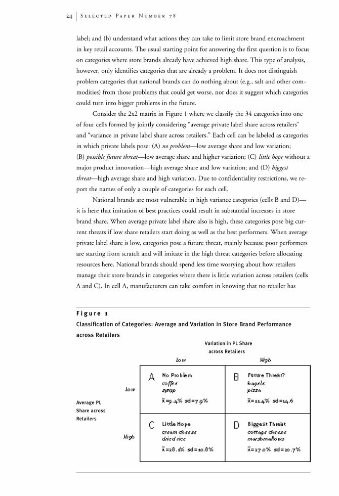
Consider the 2x2 matrix in Figure 1 where we classify the 34 categories into one

of four cells formed by jointly considering “average private label share across retailers”

and “variance in private label share across retailers.” Each cell can be labeled as categories

in which private labels pose: (A) no problem—low average share and low variation;

(B) possible future threat—low average share and higher variation; (C) little hope without a

major product innovation—high average share and low variation; and (D) biggest

threat—high average share and high variation. Due to confidentiality restrictions, we re-

port the names of only a couple of categories for each cell.

National brands are most vulnerable in high variance categories (cells B and D)—

it is here that imitation of best practices could result in substantial increases in store

brand share. When average private label share also is high, these categories pose big cur-

rent threats if low share retailers start doing as well as the best performers. When average

private label share is low, categories pose a future threat, mainly because poor performers

are starting from scratch and will imitate in the high threat categories before allocating

resources here. National brands should spend less time worrying about how retailers

manage their store brands in categories where there is little variation across retailers (cells

A and C). In cell A, manufacturers can take comfort in knowing that no retailer has

F i g u r e 1

Classification of Categories: Ave rage and Variation in St o re Brand Pe r f o r m a n c e

a c ross Re t a i l e r s

Variation in PL S h a re

a c ross Re t a i l e r s

Ave rage PL

S h a re acro s s

Re t a i l e r s

D h a r a n d H o c h 25

figured out how to sell store brands in these categories, and therefore allocate resources

against their national competitors. Cell C represents categories where private label share

growth probably has peaked, having reached a natural asymptote. And instead of over-

spending on push promotions that the retailer can arbitrage through forward buying

and diversion or pull tactics that do not work anymore, manufacturers (at least the lead-

ing brands) may get higher returns by investing in the type of product innovations that

got them where they were in the first place. Although the above analysis may serve as a

useful decision support tool for national brand manufacturers, it is important to note

that our analysis assumes that private label quality will remain comparable to that in the

existing market. However, discontinuous increases in store brand quality can occur.

Witness the successful introduction of quality cola to the soft drink market by COTT,

which posed an immediate threat to national brands in an otherwise low share, low

variation “no problem” category.

Table 6 contrasts the substantive impact of each of the independent variables for

the following three category groups: all categories (same as in Table 4); biggest threat

(cell D); and little hope (cell C). Store brands have an important position in both the

“big threat” and “little hope” categories; the difference is that variation in performance

across retailers is about four times greater in the “big threat” categories (average s2 of

.047 vs .012). Because of greater variation in the dependent variable, it is not surprising

that most of the independent variables have a greater impact on performance in the

high variance categories. Table 6 shows that brand competition variables (#BRANDS,

BRNDVAR, AVGSKU) have about two times the impact in the “high threat” categories,

suggesting that reductions in assortment could lead to big increases in store brand share.

Most of the retailer variables (SIZE, PLSKU, QUAL, PLNAME, EDLP, PREMIUM,

PRDIFF) also have substantially more impact in the “big threat” categories compared

to either the “all” category or “little” averages. In contrast, manufacturer pull tactics

(ADVPROMO) make more of a difference in the “little hope” categories, a finding for

which we do not have a ready explanation.

Although our study provides a number of interesting insights, its limitations sug-

gest several issues for future research. First, we could not obtain a direct measure of the

quality of each retailers’ store brands, a variable the previous research has shown is very

important. Our two quality-type random coefficient pooling approach provides us with

an overall picture of how a large set of characteristics influence store brand performance;

but we have not systematically modelled how these underlying relationships (represented

by the slope coefficients) might vary with other category distinctions. However, given the

large number of characteristics we consider (many of which are themselves category de-

scriptors) and lack of a theoretical framework for how the slopes might vary by category,

we feel that more could be gained by supplanting our rich but admittedly descriptive ap-

proach with a more elemental structural model (e.g., Allenby and Rossi, 1991). Finally,

although we have adjusted our econometrics to deal with endogeneity whenever we could

clearly identify it, data on about half of our variables was available on an annual level for

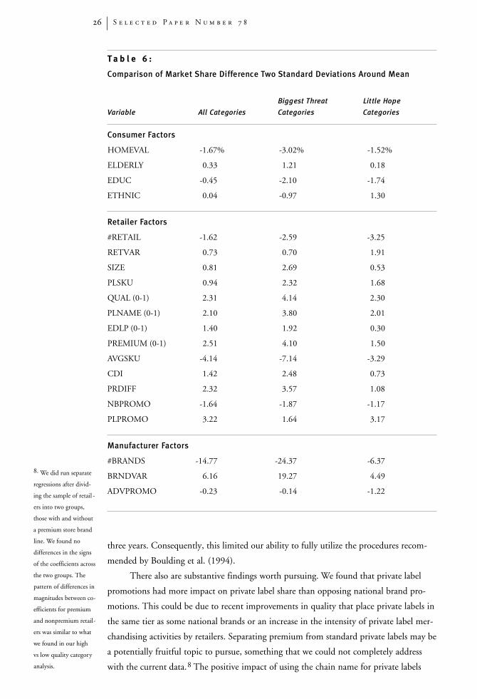
S e l e c t e d P a p e r N u m b e r 7 826

three years. Consequently, this limited our ability to fully utilize the procedures recom-

mended by Boulding et al. (1994).

There also are substantive findings worth pursuing. We found that private label

promotions had more impact on private label share than opposing national brand pro-

motions. This could be due to recent improvements in quality that place private labels in

the same tier as some national brands or an increase in the intensity of private label mer-

chandising activities by retailers. Separating premium from standard private labels may be

a potentially fruitful topic to pursue, something that we could not completely address

with the current data.8 The positive impact of using the chain name for private labels

T a b l e 6 :

Comparison of Market Share Difference Two St a n d a rd Deviations Around Mean

Biggest T h re a t Little Hope

Va r i a b l e All Categories C a t e g o r i e s C a t e g o r i e s

Consumer Fa c t o r s

HOMEVAL -1.67% -3.02% -1.52%

ELDERLY 0.33 1.21 0.18

EDUC -0.45 -2.10 -1.74

ETHNIC 0.04 -0.97 1.30

Retailer Fa c t o r s

#RETAIL -1.62 -2.59 -3.25

RETVAR 0.73 0.70 1.91

SIZE 0.81 2.69 0.53

PLSKU 0.94 2.32 1.68

QUAL (0-1) 2.31 4.14 2.30

PLNAME (0-1) 2.10 3.80 2.01

EDLP (0-1) 1.40 1.92 0.30

PREMIUM (0-1) 2.51 4.10 1.50

AVGSKU -4.14 -7.14 -3.29

CDI 1.42 2.48 0.73

PRDIFF 2.32 3.57 1.08

NBPROMO -1.64 -1.87 -1.17

PLPROMO 3.22 1.64 3.17

M a n u f a c t u rer Fa c t o r s

#BRANDS -14.77 -24.37 -6.37

BRNDVAR 6.16 19.27 4.49

ADVPROMO -0.23 -0.14 -1.22

8. We did run separate

regressions after divid-

ing the sample of retail -

ers into two groups,

those with and without

a premium store brand

line. We found no

differences in the signs

of the coefficients across

the two groups. The

pattern of differences in

magnitudes between co-

efficients for premium

and nonpremium retail-

ers was similar to what

we found in our high

vs low quality category

analysis.

D h a r a n d H o c h 27

across categories warrants further investigation into the individual cross-category purchas-

ing behavior of consumers and the impact on retailers’ image. The importance of the

#BRANDS and the AVGSKU variable suggests that national manufacturers could benefit

from a more detailed examination of the economics of using brand-extension and flanker

strategies versus line-extension strategies. Future research at an individual store and cate-

gory level needs to investigate the impact of changing the price gap between national

brands and the private label.

Finally, our results are decidedly bound to the U.S. grocery market. It is well-

known that store brands play a more dominant role is several European markets and

Canada. For example, store brands have 45 percent share in Switzerland, 37 percent in

the UK, and 22 percent in Canada. Moreover, store brands in many European markets

are reputed to be of much higher quality than in U.S., and so some might argue that the

regularities we found in the U.S. are less relevant to other markets. We have no problem

accepting the fact that the rules are not exactly the same as in the U.S. For example, re-

tail concentration is much higher in Europe (three firm concentration ratio ranging from

45 to 80 percent vs 17 percent in the U.S.). At the same time, however, the extent of

variation in store brand performance across countries is not that different in magnitude

from what we observe within the U.S. We look forward to examining these issues in

other markets as data become available.

Our research shows that the substantial differences that exist across retailers system-

atically affect the success of a chain’s private label program. Not controlling for this in

empirical studies can lead to biased conclusions (e.g., effect of national brand-private

label price differential on private label share). The study also identifies a set of basic fac-

tors describing the retailers’ strategy that account for the differential success of their pri-

vate label programs. Our research ser ves as the starting point for future inquiry that

formally recognizes the leading role of the retailer in the store brand equation.

R e f e r e n c e s

Allenby, Greg M., and Peter E. Rossi. 1991. “Quality Perceptions and Asymmetric Switching

Between Brands,” Marketing Science, 10 (3), 185–204.

Bass, Frank M., and Dick R. Wittink. 1975. “Pooling Issues and Methods in Regression Analysis

with Examples in Marketing Research,” Journal of Marketing Research, 12 (4), 414–25.

———. 1978. “Pooling Issues and Methods in Regression Analysis with Examples in Marketing

Research: Some Further Reflections,” Journal of Marketing Research, 15 (2), 277–9.

Becker, Gary. 1965. “A Theory of the Allocation of Time,” Economic Journal, 75, 493–517.

Blattberg, Robert C., Gary D. Eppen, and Joshua Lieberman. 1978. “A Theoretical and

Empirical Evaluation of Price Deals for Consumer Nondurables,” Journal of Marketing,

45 (1), 116–29.

S e l e c t e d P a p e r N u m b e r 7 828

Boulding, William, and Richard Staelin. 1995. “Identifying Generalized Effects of Strategic

Actions on Firm Performance: The Case of Demand-side Returns to R&D Spending,”

Marketing Science, 14 (3), G222–G236.

Drèze, Xavier. 1995. “Loss Leaders and Cherry Picking: A Theoretical and Empirical Analysis,”

Unpublished Dissertation, University of Chicago, Graduate School of Business.

Hausmann, J. A. 1978. “Specification Tests in Econometrics,” Econometrica, 46 (6), 1251–71.

Hoch, Stephen J. 1996. “How Should National Brands Think about Private Labels?” Sloan

Management Review, 37 (Winter), 89–102.

Hoch, Stephen J., and Shumeet Banerji. 1993. “When Do Private Labels Succeed?” Sloan

Management Review, 34 (Summer), 57–68.

Hoch, Stephen J., Xavier Drèze, and Mary E. Purk. 1994. “EDLP, Hi-Lo, and Margin Arithmetic,”

Journal of Marketing, 58 (4), 16–29.

Hoch, Stephen J., Byung-Do Kim, Alan L. Montgomery, and Peter E. Rossi. 1995. “Determinants

of Store-Level Price Elasticity,” Journal of Marketing Research, 32 (1), 17–29.

Johnston, Jack. 1984. Econometric Methods, New York: McGraw-Hill.

Judge, George, et al. 1985. The Theory and Practice of Econometrics, New York: Wiley and Sons.

Kamakura, Wagner A., and Gary J. Russell. 1989. “A Probabilistic Choice Model for Market

Segmentation and Elasticity Structure,” Journal of Marketing Research, 26 (November), 379–90.

Lal, Rajiv. 1990. “Manufacturer Trade Deals and Retail Price Promotions,” Journal of Marketing

Research, 27 (4), 428–44.

Mills, David E. 1995. “Why Do Retailers Sell Private Label?” Journal of Economics and Management

Strategy, 4 (3), 509–28.

Raju, Jagmohan S., Raj K. Sethuraman, and Sanjay K. Dhar. 1995a. “The Introduction and

Performance of Store Brands,” Management Science, 41 (June), 957–78.

———. 1995b. “National-Store Brand Price Differential and Store Brand Market Share,” Pricing

Theory & Practice, 3 (2), 17–24.

Schmalensee, Richard. 1978. “Entry-Deterrence in the Ready to Eat Breakfast Cereals Industry,”

Bell Journal of Economics, 9, 305–27.

Sethuraman, Raj. 1992. “The Effect of Marketplace Factors on Private Label Penetration in Grocery

Products,” Marketing Science Institute, Report #92-128.

Spencer, David E., and Kenneth N. Berk. 1981. “A Limited Information Specification Test,”

Econometrica, 49 (4), 1079–1086.

Starzynski, Greg. 1993. The Private Label Consumer: Is There One? Northbrook, IL: A. C. Nielsen.

Waterson, Michael. 1984. Economic Theory of the Industry, Cambridge: Cambridge University Press.

White, Hal 1980. “A Heteroskedasticity-Consistent Covariance Matrix Estimator and a Direct

Test for Heteroskedasticity,” Econometrica, 50, 483–99.