Embed Size (px)
Citation preview

Semidefinite Programming Duality andLinear Time-invariant Systems
Venkataramanan (Ragu) BalakrishnanSchool of ECE, Purdue University
2 July 2004Workshop on Linear Matrix Inequalities in Control
LAAS-CNRS, Toulouse, France

Semidefinite Programming Duality andLinear Time-invariant Systems
Venkataramanan (Ragu) BalakrishnanSchool of ECE, Purdue University
2 July 2004Workshop on Linear Matrix Inequalities in Control
LAAS-CNRS, Toulouse, France
Joint work with Lieven Vandenberghe, UCLA
SDP DUALITY AND LTI SYSTEMS 1
Basic ideas
• Many control constraints yield LMIs, many control problems are SDPs

SDP DUALITY AND LTI SYSTEMS 1
Basic ideas
• Many control constraints yield LMIs, many control problems are SDPs
• LMIs are convex constraints, SDPs are convex optimization problems
• From duality theory in convex optimization:
? Theorem of alternatives for LMIs
? SDP duality

SDP DUALITY AND LTI SYSTEMS 1
Basic ideas
• Many control constraints yield LMIs, many control problems are SDPs
• LMIs are convex constraints, SDPs are convex optimization problems
• From duality theory in convex optimization:
? Theorem of alternatives for LMIs
? SDP duality
• Explore implication of convex duality theory on underlying control problem:
? New (often simpler) proofs for classical results
? Some new results

SDP DUALITY AND LTI SYSTEMS 2
LMIs and Semidefinite Programming
• V is a finite-dimensional Hilbert space, S is a subspace of Hermitianmatrices, F : V → S is a linear mapping, F0 ∈ S
• Inequality F(x) + F0 ≥ 0 is an LMI
• SDP is an optimization of the form:
minimize: 〈c, x〉Vsubject to: F(x) + F0 ≥ 0
SDP DUALITY AND LTI SYSTEMS 3
A theorem of alternatives for LMIs
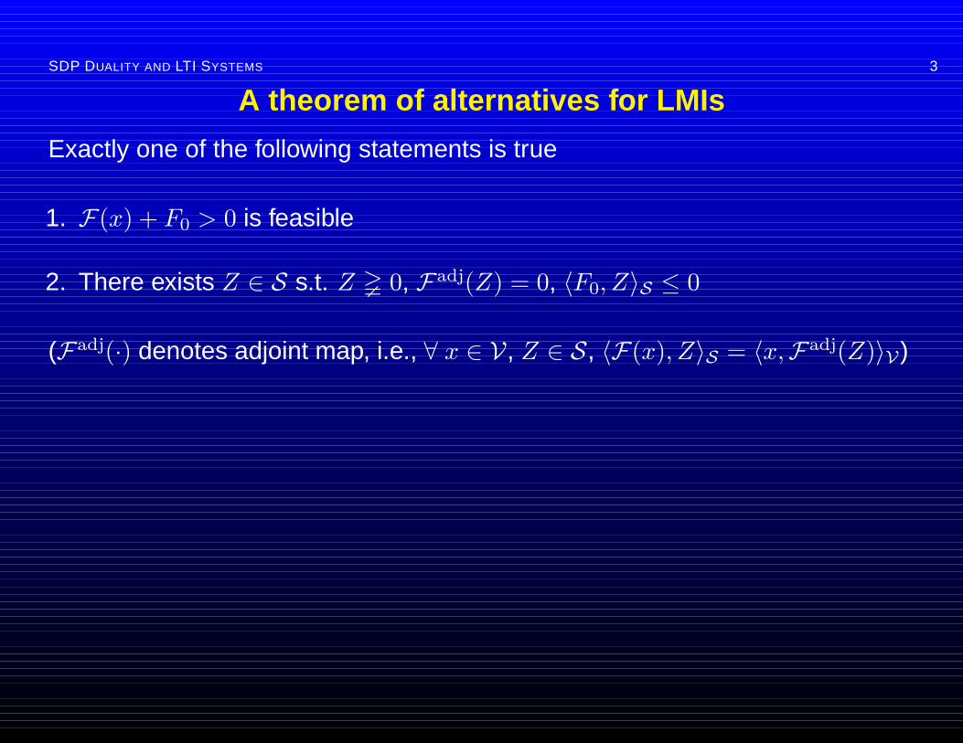
Exactly one of the following statements is true
1. F(x) + F0 > 0 is feasible
2. There exists Z ∈ S s.t. Z 0, Fadj(Z) = 0, 〈F0, Z〉S ≤ 0
(Fadj(·) denotes adjoint map, i.e., ∀ x ∈ V, Z ∈ S, 〈F(x), Z〉S = 〈x,Fadj(Z)〉V)

SDP DUALITY AND LTI SYSTEMS 3
A theorem of alternatives for LMIs
Exactly one of the following statements is true
1. F(x) + F0 > 0 is feasible
2. There exists Z ∈ S s.t. Z 0, Fadj(Z) = 0, 〈F0, Z〉S ≤ 0
(Fadj(·) denotes adjoint map, i.e., ∀ x ∈ V, Z ∈ S, 〈F(x), Z〉S = 〈x,Fadj(Z)〉V)
• Variants available for nonstrict inequalities such as F(x) + F0 0 andF(x) + F0 ≥ 0, and with additional linear equality constraints F(x) = 0
• Typically get weak alternatives, need additional conditions (constraintqualifications) to make them strong
SDP DUALITY AND LTI SYSTEMS 4
Proof of theorem of alternatives
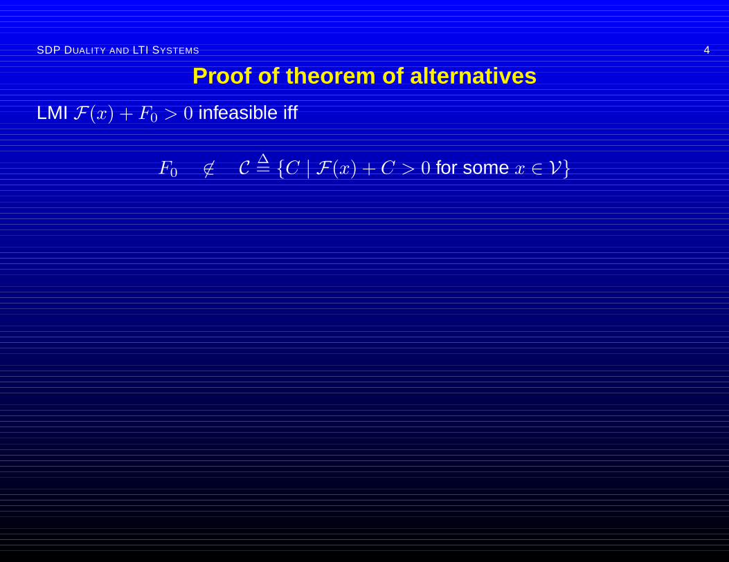
LMI F(x) + F0 > 0 infeasible iff
F0 6∈ C ∆= {C | F(x) + C > 0 for some x ∈ V}

SDP DUALITY AND LTI SYSTEMS 4
Proof of theorem of alternatives
LMI F(x) + F0 > 0 infeasible iff
F0 6∈ C ∆= {C | F(x) + C > 0 for some x ∈ V}
C is open, nonempty and convex, so there exists hyperplane strictly separtingF0 and C:
∃Z 6= 0 s.t. 〈F0, Z〉S < 〈C,Z〉S for all C ∈ C

SDP DUALITY AND LTI SYSTEMS 4
Proof of theorem of alternatives
LMI F(x) + F0 > 0 infeasible iff
F0 6∈ C ∆= {C | F(x) + C > 0 for some x ∈ V}
C is open, nonempty and convex, so there exists hyperplane strictly separtingF0 and C:
∃Z 6= 0 s.t. 〈F0, Z〉S < 〈C,Z〉S for all C ∈ C
∃Z 6= 0 s.t. 〈F0, Z〉S < 〈−F(x) + X, Z〉S for all x ∈ V, X > 0
∃Z 6= 0 s.t. 〈F0, Z〉S < 〈x,−Fadj(Z)〉V + 〈X, Z〉S for all x ∈ V, X > 0
Thus, there exists Z ∈ S s.t. Z 0, Fadj(Z) = 0, 〈F0, Z〉S ≤ 0

SDP DUALITY AND LTI SYSTEMS 5
Application: A Lyapunov inequality
• LMI A∗P + PA < 0 is feasible, or
• There exists Z s.t. Z 0, AZ + ZA∗ = 0
Factoring Z = UU∗, can show
AU = US, S has pure imaginary eigenvalues
Thus:
LMI A∗P + PA < 0 is infeasible if and only if A has a pure imaginaryeigenvalue

SDP DUALITY AND LTI SYSTEMS 6
Other results
• “P > 0, A∗P + PA < 0” is infeasible iff λi(A) ≥ 0 for some i
• “A∗P + PA � 0” is infeasible iff A is similar to a purely imaginary diagonalmatrix
• “A∗P + PA ≤ 0, P 0” is infeasible iff λi(A) ≥ 0 for all i
• “A∗P + PA � 0, PB = 0” is infeasible iff all uncontrollable modes of (A,B)are nondefective and correspond to imaginary eigenvalues
• “P 0, A∗P + PA ≤ 0, PB = 0” is infeasible iff all uncontrollable modes of(A,B) correspond to eigenvalues with positive real part
• “P 6= 0, A∗P + PA ≤ 0, PB = 0” is infeasible iff (A,B) is controllable

SDP DUALITY AND LTI SYSTEMS 7
Frequency-domain inequalities: The KYP Lemma
Inequalities of the form[(jωI −A)−1B
I
]∗M
[(jωI −A)−1B
I
]> 0
are commonly encountered in systems and control:
• Linear system analysis and design
• Digital filter design
• Robust control analysis
• Examples of constraints: |H(jω)| < 1 (small gain), <H(jω) > 0 (passivity),H(jω) + H(jω)∗ + H(jω)∗H(jω) < 1 (mixed constraints)

SDP DUALITY AND LTI SYSTEMS 8
The Kalman-Yakubovich-Popov Lemma
FDI [(jωI −A)−1B
I
]∗M
[(jωI −A)−1B
I
]> 0
holds for all ω iff LMI [A∗P + PA PB
B∗P 0
]−M < 0
is feasible
• Infinite-dimensional constraint reduced to finite-dimensional constraint
• No sampling in frequency required

SDP DUALITY AND LTI SYSTEMS 9
Control-theoretic proof of KYP Lemma
Suppose LMI [A∗P + PA PB
B∗P 0
]−M < 0
is feasible
Then
0 <
[(jωI −A)−1B
I
]∗(M −
[A∗P + PA PB
B∗P 0
]) [(jωI −A)−1B
I
]=
[B∗(−jωI −A∗)−1 I
]M
[(jωI −A)−1B
I
]

SDP DUALITY AND LTI SYSTEMS 9
Control-theoretic proof of KYP Lemma
Suppose LMI [A∗P + PA PB
B∗P 0
]−M < 0
is feasible
Then
0 <
[(jωI −A)−1B
I
]∗(M −
[A∗P + PA PB
B∗P 0
]) [(jωI −A)−1B
I
]=
[B∗(−jωI −A∗)−1 I
]M
[(jωI −A)−1B
I
]
Converse much harder; based on optimal control theory

SDP DUALITY AND LTI SYSTEMS 10
New KYP lemma proof
More general version of the KYP Lemma:
Suppose M22 > 0 [A∗P + PA PB
B∗P 0
]−M < 0,
is feasible iff
(jωI −A)u = Bv, (u, v) 6= 0 =⇒[
u∗ v∗]M
[uv
]> 0
• A can have imaginary eigenvalues
• If A has no imaginary eigenvalues, recover classical version

SDP DUALITY AND LTI SYSTEMS 11
Duality-based KYP Lemma proof
Infeasibility of [A∗P + PA PB
B∗P 0
]−M < 0
equivalent to existence of Z s.t.
Z =[
Z11 Z12
Z∗12 Z22
] 0, Z11A
∗ + AZ11 + Z12B∗ + BZ∗12 = 0, TrZM ≤ 0
• Must have Z11 0. Hence, factor Z as
[Z11 Z12
Z∗12 Z22
]=
[U 0V V
] [U∗ V ∗
0 V ∗
],
where U has full rank

SDP DUALITY AND LTI SYSTEMS 12
• Can show
US −AU = BV, Tr([
U∗ V ∗]M
[UV
])≤ 0,
with S + S∗ = 0
• Take Schur decomposition of S: S =∑m
i=1 jωiqiq∗i , with
∑i qiq
∗i = I
• Then
q∗k[
U∗ V ∗]M
[UV
]qk ≤ 0
for some k
• Define u = Uqk, v = V qk. Then
[u∗ v∗
]M
[uv
]≤ 0 and (jωI −A)u = Bv

SDP DUALITY AND LTI SYSTEMS 13
Outline
• Theorem of alternatives for LMIs, and their applications
• SDP duality, and its application

SDP DUALITY AND LTI SYSTEMS 14
Primal and dual SDPs
Primal SDP:minimize: 〈c, x〉Vsubject to: F(x) + F0 ≥ 0
Dual SDPmaximize −〈F0, Z〉Ssubject to Fadj(Z) = c, Z ≥ 0
• If Z is dual feasible, then −TrF0Z ≤ p∗
• If x is primal feasible, then cTx ≥ d∗
• Under mild conditions, p∗ = d∗
• At optimum, (F(xopt) + F0) Zopt = 0

SDP DUALITY AND LTI SYSTEMS 15
Application of duality: Bounds on H∞ normStable LTI system
x = Ax + Bu, x(0) = 0, y = Cx
• Transfer function H(s) = C(sI −A)−1B
• H∞ norm of H defined as
‖H‖∞ = sup<s>0
σmax(H(s))
• ‖H‖2∞ equals maximum energy gain
‖H‖2∞ = max
u
∫yTy∫uTu

SDP DUALITY AND LTI SYSTEMS 16
‖H‖∞ computation as an SDP
minimize: β
subject to:
[A∗P + PA + C∗C PB
B∗P −βI
]≤ 0
(‖H‖2∞ = βopt)
Dual problem
maximize: TrCZ11C∗
subject to: Z11A∗ + AZ11 + Z12B
∗ + BZ∗12 = 0[Z11 Z12
Z∗12 Z22
]≥ 0, TrZ22 = 1
SDP DUALITY AND LTI SYSTEMS 17
Control-theoretic interpretation of dual problem
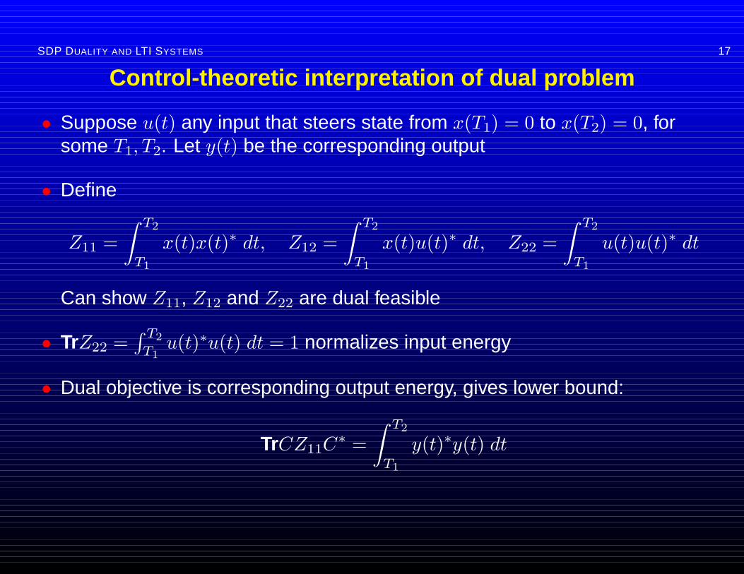
• Suppose u(t) any input that steers state from x(T1) = 0 to x(T2) = 0, forsome T1, T2. Let y(t) be the corresponding output
• Define
Z11 =∫ T2
T1
x(t)x(t)∗ dt, Z12 =∫ T2
T1
x(t)u(t)∗ dt, Z22 =∫ T2
T1
u(t)u(t)∗ dt
Can show Z11, Z12 and Z22 are dual feasible
• TrZ22 =∫ T2
T1u(t)∗u(t) dt = 1 normalizes input energy
• Dual objective is corresponding output energy, gives lower bound:
TrCZ11C∗ =
∫ T2
T1
y(t)∗y(t) dt
SDP DUALITY AND LTI SYSTEMS 18
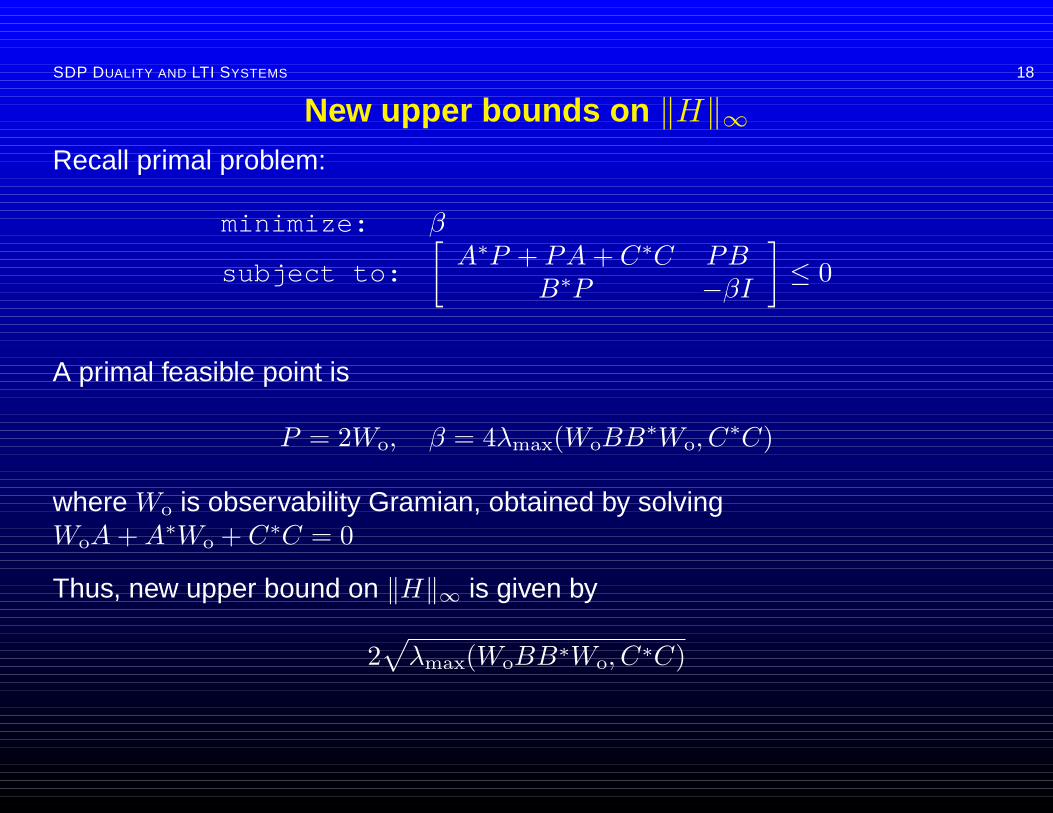
New upper bounds on ‖H‖∞Recall primal problem:
minimize: β
subject to:
[A∗P + PA + C∗C PB
B∗P −βI
]≤ 0
A primal feasible point is
P = 2Wo, β = 4λmax(WoBB∗Wo, C∗C)
where Wo is observability Gramian, obtained by solvingWoA + A∗Wo + C∗C = 0
Thus, new upper bound on ‖H‖∞ is given by
2√
λmax(WoBB∗Wo, C∗C)

SDP DUALITY AND LTI SYSTEMS 19
New lower bounds on ‖H‖∞Recall dual problem
maximize: TrCZ11C∗
subject to: Z11A∗ + AZ11 + Z12B
∗ + BZ∗12 = 0[Z11 Z12
Z∗12 Z22
]≥ 0, TrZ22 = 1
A dual feasible point is
Z11 = Wc/α, Z12 = B/(2α), Z22 = B∗W−1c B/(4α),
where α = Tr(B∗W−1c B/4)
Thus new lower bound is
2√
TrCWcC∗/(TrB∗W−1c B)

SDP DUALITY AND LTI SYSTEMS 20
Application of duality: LQR problem
Primal
minimize: TrQZ11 + TrZ22
subject to: AZ11 + BZ∗12 + Z11A∗ + Z12B
∗ + x0x∗0 ≤ 0,[
Z11 Z12
Z∗12 Z22
]≥ 0
Dualmaximize: x∗0Px0
subject to:
[A∗P + PA + Q PB
B∗P I
]≥ 0, P ≥ 0

SDP DUALITY AND LTI SYSTEMS 21
The Linear-Quadratic Regulator problem
x = Ax + Bu, x(0) = x0,
find u that minimizes J =∫ ∞
0
(x(t)∗Qx(t) + u(t)∗u(t)) dt,
s.t. limt→∞ x(t) = 0
Well-known solution: Solve Riccati equation
ATP + PA + Q− PBBTP = 0
such that P > 0. Then,uopt(t) = −BTPx(t)
(Proof using quadratic optimal control theory)

SDP DUALITY AND LTI SYSTEMS 22
Duality-based proof: Basic ideas
• Primal problem gives upper bound on LQR objective
• Dual problem gives lower bound on LQR objective
• Optimality condition gives LQR Riccati equation

SDP DUALITY AND LTI SYSTEMS 23
Primal problem interpretation
Assume u = Kx, s.t. x(t) → 0 as t →∞
Then LQR objective reduces to
JK =∫ ∞
0
x(t)∗ (Q + K∗K) x(t) dt
and is an upper bound on the optimum LQR objective
• Condition x(t) → 0 as t →∞ equivalent to
(A + BK)Z + Z(A + BK)∗ + x0x∗0 = 0, Z ≥ 0
• LQR objective is TrZ(Q + K∗K)

SDP DUALITY AND LTI SYSTEMS 24
Best upper bound using state-feedback:
minimize: TrZ(Q + K∗K)subject to: Z ≥ 0
(A + BK)Z + Z(A + BK)∗ + x0x∗0 = 0
With Z11 = Z, Z12 = ZK∗, Z22 = KZK∗:
minimize: TrQZ11 + TrZ22
subject to: AZ11 + BZ∗12 + Z11A∗ + Z12B
∗ + x0x∗0 ≤ 0,[
Z11 Z12
Z∗12 Z22
]≥ 0
(Same as primal problem)
SDP DUALITY AND LTI SYSTEMS 25
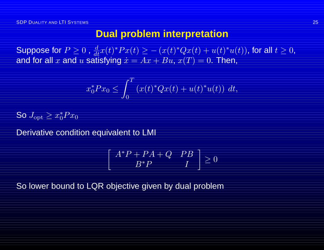
Dual problem interpretation
Suppose for P ≥ 0 , ddtx(t)∗Px(t) ≥ − (x(t)∗Qx(t) + u(t)∗u(t)), for all t ≥ 0,
and for all x and u satisfying x = Ax + Bu, x(T ) = 0. Then,
x∗0Px0 ≤∫ T
0
(x(t)∗Qx(t) + u(t)∗u(t)) dt,
So Jopt ≥ x∗0Px0
Derivative condition equivalent to LMI[A∗P + PA + Q PB
B∗P I
]≥ 0
So lower bound to LQR objective given by dual problem

SDP DUALITY AND LTI SYSTEMS 26
Optimality conditions
• Stabilizability of (A,B) guarantees strict primal feasibility
• Detectability of (Q,A) guarantees strict dual feasibility
• Recall, at optimality (F(xopt) + F0) Zopt = 0. This becomes[Z11 Z12
Z∗12 Z22
] [A∗P + PA + Q PB
B∗P I
]= 0
Reduces to [I K∗ ] [
A∗P + PA + Q PBB∗P I
]= 0,
or K = −B∗P , with all the eigenvalues of A + BK having negative realpart, and
A∗P + PA + Q− PBB∗P = 0(Classical LQR result, derived using duality)

SDP DUALITY AND LTI SYSTEMS 27
Conclusions
• SDP duality theory has interesting implications systems and control
• Implications for numerical computation:
? Dual problems sometimes have fewer variables
? Most efficient algorithms solve primal and dual together; control-theoreticinterpretation can help increase efficiency