Screening in Contract Design:

Evidence from the ACA Health Insurance Exchanges∗

Michael Geruso† Timothy Layton‡ Daniel Prinz§

May 2, 2018

Abstract

We study insurers’ use of prescription drug formularies to screen consumers in the ACA HealthInsurance Exchanges. We begin by showing that Exchange risk adjustment and reinsurance suc-ceed in neutralizing selection incentives for most, but not all, consumer types. A minority ofconsumers, identifiable by demand for particular classes of prescription drugs, are predictablyunprofitable. We then show that contract features relating to these drugs are distorted in a man-ner consistent with multi-dimensional screening. The empirical findings support a long theoreticalliterature examining how insurance contracts offered in equilibrium can fail to optimally trade-offrisk protection and moral hazard.

∗We thank Naoki Aizawa, Marika Cabral, Colleen Carey, Jeff Clemens, Leemore Dafny, Kurt Lavetti, Tom McGuire, RitaSantos, Mark Shepard, Amanda Starc and seminar and meeting participants at the American-European Health EconomicsStudy Group, the University of Arizona, the Caribbean Health Economics Symposium, the Federal Trade Commission,Harvard Medical School, Hunter College, the Kellogg Healthcare Markets Conference, the NBER Insurance Working GroupMeeting, the NBER Summer Institute Health Care Meeting, the Penn-LDI Health Insurance Exchange Conference, theTulane Conference on Behavior and Innovation in Healthcare, the United States Congress, and UT Austin for helpfulfeedback. We gratefully acknowledge financial support from center grants P2C HD042849 and T32 HD007081 awarded tothe Population Research Center at the University of Texas at Austin by the Eunice Kennedy Shriver National Institute ofChild Health and Human Development (Geruso), a center grant for work on "Selection Incentives in Health Plan Design"awarded by Pfizer (Geruso, Layton, Prinz), financial support from the National Institute of Mental Health (R01-MH094290,T32-019733) (Layton), and additional financial support from the Laura and John Arnold Foundation (Layton). The contentis solely the responsibility of the authors and does not necessarily represent the official views of any funder. No party hadthe right to review this paper prior to its circulation.

†University of Texas at Austin and NBER. Email: mike.geruso@gmail.com‡Harvard Medical School and NBER. Email: layton@hcp.med.harvard.edu§Harvard University. Email: dprinz@g.harvard.edu

1 Introduction

The Patient Protection and Affordable Care Act (ACA) of 2010 significantly altered the structure of

the individual and small group health insurance markets in the United States. In establishing the

new health insurance Exchanges, the ACA created a system that largely resembles managed com-

petition in Medicare Parts C and D and in health insurance markets throughout the OECD. Two

hallmark features of these markets are that no consumer can be denied coverage and that plans can-

not price discriminate based on an individual’s health status. This ban against price discrimination

on pre-existing conditions continues to play a central role in debates over the future of the individual

markets. Proposals to repeal the ACA often explicitly highlight an intention to maintain protections

for consumers with pre-existing conditions.

Enforcing a policy of no price discrimination against the chronically ill can generate improve-

ments in both equity and efficiency (Handel, Hendel and Whinston, 2015). But such reforms may

also generate a relationship between non-contractible consumer characteristics and the underlying

cost to the insurer of providing coverage. In such settings, two classes of distortions may arise. The

first is a price distortion caused by adverse selection of consumers on price, as originally studied by

Akerlof (1970).1 The second—the focus of this paper—is a distortion of insurance contract features

like risk protection and multidimensional quality. This type of distortion was first studied by Roth-

schild and Stiglitz (1976) and more recently applied to the context of modern health insurance by

Azevedo and Gottlieb (2017), Frank, Glazer and McGuire (2000), Glazer and McGuire (2000), and

Veiga and Weyl (2016).2 Under this type of distortion, insurers recognize that non-price features of

the contract can act as screening mechanisms, inducing consumers to self-sort by profitability. The

screening incentive drives a wedge between the contracts offered by insurers in equilibrium and the

socially-optimal contract that efficiently trades off risk protection and moral hazard. Although the

theoretical importance of both types of distortions is well-established, empirical evidence has largely

focused on price distortions.

In this paper, we add to the small body of empirical evidence on non-price contract distortions.

We examine the design of prescription drug formularies in the context of the individual health in-

1For recent empirical applications, see Einav, Finkelstein and Cullen (2010), Handel, Hendel and Whinston (2015), andHackmann, Kolstad and Kowalski (2015).

2Azevedo and Gottlieb (2017) show that this second class of distortion can actually be thought of as a version of thefirst class, where the contract space is large and certain contracts in that space would face complete death spirals if offered,resulting in their non-existence in equilibrium.

1

surance markets that were reformed by the ACA. Pharmaceuticals for managing chronic illness are

likely to be among the most price-transparent and predictable medical goods that healthcare con-

sumers encounter. This implies that formulary benefit design—i.e., how plans arrange prescription

medication coverage into various cost-sharing tiers—may be particularly salient to consumers, and

therefore particularly effective as a screening tool.3

We begin our study of this issue by systematically examining whether prescription drug utiliza-

tion represents a plausible screening mechanism for patient profitability. Identifying patient prof-

itability in this setting requires accounting for the regulatory transfers aimed at compensating plans

for enrolling costly consumers. Risk adjustment transfers and reinsurance were introduced into the

individual markets by the ACA with this purpose. These payment mechanisms imply that an in-

surer’s net revenues can vary substantially across enrollees who pay the same premiums. Drawing

on a large sample of health claims, we use the Exchange regulator’s risk adjustment and reinsurance

algorithms to simulate enrollee-specific net revenue from data on expenditures and diagnoses. We

compare the simulated Exchange revenues to the directly observed claims costs, yielding estimates

of person-specific implied profits. To understand the potential for screening unprofitable patient

types on the basis of drug coverage, we group patients by prescription drug consumption in various

therapeutic classes.4

As a first result, we show that while there is significant variation in expected insurer costs for

individuals taking drugs in different therapeutic classes, expected insurer profits are similar across

the vast majority of patient types, in line with the regulatory goal. For example, consider a consumer

who fills a prescription for a vasodilating agent to treat angina, a symptom of coronary artery disease.

In our data, such a consumer has expected annual medical spending around $24,000, which is far

above premiums. But that consumer generates revenues of around $26,000 after accounting for the

regulatory transfer payments. These transfers represent a regulatory success in that they neutralize

the incentive for an insurer to discourage enrollment of this patient type—for example, by restricting

access to these drugs. In fact, we find the average relationship between total medical spending and

3In a study of HIV medication access, Jacobs and Sommers (2015) show that Exchange plans in several states haveplaced an entire class of commonly-prescribed HIV medications, including generic medications, on a high cost-sharingtier. Such benefit design choices are plausibly an attempt by plans to avoid attracting enrollees with HIV. In addition,numerous lawsuits have been filed against insurers by patient advocacy groups for similar formulary design choices.

4Rather than focus on individual drug products, the universe of drugs is partitioned into groups of standard therapeuticclasses. This allows us to differentiate between a plan attempting to screen out a patient and a plan attempting to steer apatient to lower cost or higher cost-effectiveness alternatives within a class of substitutes.

2

profitability across drug class types to be approximately zero.

Despite that for most consumer types selection incentives are neutralized, we also find that “pay-

ment errors” exist for a small number of drug classes. In some cases, costs exceed revenues and in

others vice versa. For these outlier cases, the insurer screening incentives can be significant. A con-

sumer taking a drug in the biological response modifiers class (such as Copaxone, which treats multiple

sclerosis), is among the most unprofitable in our data. Such a consumer on average will generate

$61,000 in costs but only $47,000 in net revenue after accounting for the large risk adjustment and

reinsurance transfer payments to the plan enrolling her.

The existence of these types of payment errors provides a natural experiment by which we can

test how insurers respond to the signal of profitability embedded in a consumer’s demand for a

particular drug class. To leverage this experiment, we use formulary data covering every plan offered

in the state and federal Exchanges in 2015. We generate measures of coverage generosity for each

drug class for each Exchange plan. We then examine formulary design for drug classes where the

payment system is working well (i.e. average revenues match average costs) and for drug classes

where the payment system is working poorly (i.e. average revenues do not match average costs).

We compare these patterns to formulary designs in large, self insured employer plans which do not

face the same screening incentives. This difference-in-differences design allows us to control for drug

class characteristics that are difficult to measure but fixed across the two market settings, such as cost

effectiveness.

We find that insurers respond to payment system errors by designing formularies to be differen-

tially unattractive to unprofitable groups. These results are not driven by the overall lower coverage

generosity of Exchange plans. Instead, conditional on an Exchange plan’s overall generosity, drug

classes used by less profitable consumers appear higher on the formulary tier structure (implying

higher out-of-pocket costs) or are subject to more non-price barriers to access such as prior autho-

rization. The pattern is particularly stark for the tails of the distribution of selection incentives. We

find that drug classes in the upper 5% of the selection incentive distribution are about 30 percentage

points (70 percent) more likely to be placed on a specialty tier, to face utilization management, or

simply to not be covered—relative to other drugs in the same plan and relative to the same drugs in

employer plans. The associated out-of-pocket financial exposure can be significant. As we show, spe-

cialty tier coverage is likely to be governed by coinsurance rates rather than copays, implying a po-

3

tential difference of thousands of dollars in annual out of pocket spending per consumer.5 Although

throughout the paper we describe the screening problem in terms of insurer behavior (in designing

formularies), it is important to recognize that the patterns we uncover involve market forces that are

beyond any insurance carrier’s ability to control. These contract distortions are a reaction to a market

failure that has not yet been sufficiently counteracted by a regulatory response.

We perform several extensions of our analysis to show that the contract design patterns we doc-

ument among Exchange plans do not simply reflect insurers passing-through underlying drug costs

to the consumer or nudging consumers toward lower-cost substitutes. Consistent with the screening

hypothesis, we show that the relationship between payment errors and formulary restrictiveness is

strongest for the most popular drugs within an unprofitable class, possibly because coverage for such

drugs may be particularly salient in the consumer’s plan enrollment decision.

Our paper contributes both specific insights into the functioning of the Exchange risk adjustment

system and broader insights on the use of contract features as screening mechanisms. In the narrow

context of the ACA Exchanges, we show that Exchange risk adjustment and reinsurance neutralize

the selection incentives associated with most consumer types that are signaled by drug demand. We

also document, for the first time, several important facts about the design of Exchange formularies

and how these compare to formularies in employer plans. In particular, we show that Exchange

plans are far more likely to use utilization management to constrain pharmaceutical access, possibly

in part due to the ACA’s cost sharing subsidies, which constrain insurers’ options in setting out of

pocket cost sharing.

More broadly, our work connects to a long literature on screening in selection markets and the

notion of service-level selection. While several papers (Frank, Glazer and McGuire, 2000; Ellis and

McGuire, 2007; Geruso and McGuire, 2016; Layton et al., 2017) construct measures characterizing

selection incentives that vary by service type or setting, only a small recent literature (Decarolis and

Guglielmo, 2017; Shepard, 2016; Carey, 2017a,b; Lavetti and Simon, 2016) has been able to empirically

document insurer responses to such incentives in terms of contract design.6 Our work mostly closely

5For a prescription from a class like Biological Response Modifiers (which we find to be particularly unprofitable) out-of-pocket consumer costs can exceed $1,000 per month in a typical Exchange Silver plan. Such costs could push consumersup to the out-of-pocket annual maximum, which in 2016 was $6,850 for an individual plan and $13,700 for a family plan.

6Carey (2017a) and Lavetti and Simon (2016) empirically investigate a high-dimensional service-level screening problemof the type described by Frank, Glazer and McGuire (2000). Other work in the area of contract distortions has focused on asingle screen. In the context of a pre-ACA Massachusetts Exchange, Shepard (2016) investigates the inclusion of expensive"star" hospitals in plans’ networks as a screening mechanism. Decarolis and Guglielmo (2017) study how overall plangenerosity induces differential enrollment in privatized Medicare (Parts C and D), collapsing plan generosity into a single

4

aligns with that of Carey (2017a) and Lavetti and Simon (2016), which both examine formulary de-

sign in Medicare Part D. Like those papers, we find that the generosity of drug coverage tracks the

profitability of various consumer health types.7 In contrast to prior work, we find that Exchange

plan formularies appear to use non-monetary aspects of plan design in the form of utilization man-

agement, suggesting important differences between the widely studied Medicare Part D market and

the understudied individual markets.8

In addition to presenting the first econometric evidence of screening in the Exchanges, our find-

ings extend the existing literature by providing new insights regarding insurers’ sophistication in

responding to selection incentives. We show that insurers appear to look beyond drug-specific costs

when setting cost sharing schedules. Unlike in Medicare Part D standalone plans, which cover only

drugs, drug expenditure is a minority share of total healthcare spending in the plans we study. There-

fore, savvy insurers would restrict access to even cheap drugs that are associated with patients who

are expensive net of risk adjustment. This is what we find, with plans restricting access to lower cost

brand drugs and generics when demand for those drugs predicts patients who are unprofitable.9

These insights regarding insurer sophistication carry the implication—predicted by theory, but often

ignored in policy discussions—that selection incentives, and not merely high upstream pharmaceu-

tical prices, are partly responsible for the high out-of-pocket drug costs faced by US consumers in

the individual health insurance market. It is unprofitable enrollees, rather than costly ones, who are

likely to bear high out-of-pocket spending risk.

The remainder of the paper proceeds as follows. We begin in Section 2 by briefly reviewing

the theory of service-level selection and by describing the regulatory environment. In Section 3 we

describe the data, and in Section 4 we evaluate the performance of the ACA’s risk adjustment and

reinsurance programs in neutralizing selection incentives. Section 5 describes our research design,

dimension. Other related strands of research investigate insurers’ use of advertising to achieve favorable selection (Aizawaand Kim, 2015), and more direct forms of discrimination that do not necessarily operate via benefit design (Kuziemko,Meckel and Rossin-Slater, 2013).

7A related literature considers insurance coverage distortions in formularies due not to selection, but due to the potentialfor drug and medical spending to offset each other and the feature that some markets separate these kinds of coverage. SeeChandra, Gruber and McKnight (2010) and Starc and Town (2015).

8Methodologically, the technique we introduce to identify unprofitable consumer types differs from the prior empiricalliterature in allowing a direct prediction of where the contract distortions should occur without requiring an intermediatemapping of contract parameters to variables included in the risk adjustment algorithm. This is a subtle but important pointbecause it allows us to identify patient types who face discrimination but whose chronic conditions are not included in therisk adjustment formula. In our empirical context, this includes women seeking fertility treatments.

9For example, due to high inpatient and outpatient spending that isn’t fully compensated by risk adjustment and rein-surance.

5

and Section 6 reports our findings of contract distortions in the Exchanges. Sections 7 shows our

results are not easily explained by alternative hypotheses regarding efficiently steering patients to

more cost effective alternatives. Section 8 performs a simple counterfactual analysis of the effects of

dropping reinsurance from the Exchange markets. Section 9 concludes with a discussion of policy

implications and potential solutions.

2 Background

2.1 Conceptual Framework

The theory behind insurance contract distortions due to the screening incentives has been carefully

developed elsewhere, including in Rothschild and Stiglitz (1976), Frank, Glazer and McGuire (2000),

Glazer and McGuire (2000), Ellis and McGuire (2007), Veiga and Weyl (2016), and Azevedo and Got-

tlieb (2017). Our goal in this section is not to generate new theoretical insights. Rather we discuss

how this body of theory applies to the setting we study: Prescription drug formularies among Ex-

change plans. We refer the reader to Geruso and Layton (2017) for a more comprehensive treatment

of this literature.

Consider consumers of types c ∈ C, who vary in both expected healthcare spending and in

demand for particular classes of medical services. For simplicity assume a one-to-one mapping of

consumer types to healthcare services, so that c can be thought of as service types. Insurers offer

contracts that consist of service- or type-specific coinsurance rates, 1− xc, with xc ∈ [0, 1] being the

portion of spending paid by the insurer. It is straightforward to show that in a static one-period

setting, the social planner would maximize social welfare by setting each coinsurance rate, 1− x∗c ,

to balance the benefit of risk protection against the social cost of moral hazard (Zeckhauser, 1970;

Feldstein, 1973). In this same static setting, if insurers j ∈ J can set type-specific premiums pjc and

restrict enrollment into a given contract to consumers of a particular type, then competition causes

the type-specific profit-maximizing contracts, (pjc, xj

c), to be identical to the socially optimal contract

(p∗c , x∗c ).10,11

10Note that we assume that insurers have full information about consumer types, i.e. there is no asymmetric informationin the model. Type-specific contracts thus need not specify coinsurance rates for services other than the service used by theconsumer type (service c).

11When considering a dynamic or multi-period setting, transitions between health states (or types c) would lead todifferent optimal copayments (Handel, Hendel and Whinston, 2015).

6

However, the consequences of competition change when, as in the ACA Exchanges, all con-

sumers in a market are combined in a single-risk pool and insurers cannot directly discriminate via

setting type-specific premiums or via restricting particular contracts to particular types.12 As we

model in detail in Appendix A, relative to the social planner’s contract design problem, the profit-

maximizing insurer now has an additional consideration in how it sets coinsurance rates, xjc: By vary-

ing coverage for service c, the plan will attract marginal enrollees who may be differentially profitable

to the insurer depending on their type-specific costs relative to the uniform premium. Thus, the plan

now has an interest not only in providing optimal risk protection for a fixed set of enrollees, it must

also consider the set of enrollees its benefits package attracts.

The possibility of screening consumers by setting a schedule of coinsurance rates xc that are dif-

ferentially attractive across consumer types drives a wedge between the profit-maximizing coverage

levels in the single-risk pool setting and the socially efficient level of coverage. Risk adjustment can

affect the size of this wedge by shifting the relative profitability of different groups. With risk adjust-

ment, it is not the comparison between the cost of the consumer type and the uniform premium that

motivates the distortionary movement of the coinsurance rates away from the optimal rates. Rather,

it is the comparison between the cost of the consumer type and the uniform premium plus any risk

adjustment transfer the insurer receives for the type. Given the right set of risk adjustment trans-

fers, insurers could theoretically be induced to offer the socially optimal contract. In the presence of

risk adjustment “payment errors,” wedges between the socially optimal coinsurance rates and the

equilibrium rates will remain.

Though we merely sketch the intuition here, this result is shown rigorously by Glazer and McGuire

(2000), Frank, Glazer and McGuire (2000), and Veiga and Weyl (2016), who also show that the size

of the wedge is proportional to the covariance among marginal consumers between willingness-to-

pay for coverage and the consumer’s (net of risk adjustment) cost to the insurer. Ellis and McGuire

(2007) devise a practical empirical metric that reflects this covariance, which we follow below when

we empirically operationalize the insurer’s selection incentive.

Several takeaways here are important for our analysis below: First, although the theoretical liter-

ature has primarily focused on settings in which the only revenue associated with enrollees is premi-

ums, it is straightforward to observe that when additional revenues or transfer payments are present

12In this case, the insurer offers contracts specifying the full vector of type-specific coinsurance rates, xc.

7

(such as risk adjustment and reinsurance, described below), insurers should respond to the residual

incentive net of the payment system, not the gross cost of an individual. Second, in a multi-service

contract, the overall profitability of an individual to the insurer matters for the distortionary incen-

tive, not just the individual’s spending on the particular service—in our case, drugs. This means that

if an unprofitable group of consumers desires access to a cheap drug, an insurer will want to inef-

ficiently distort coverage to be poor for that cheap drug. Third, the extent of the contract distortion

should scale with the size of the selection incentive.13 Fourth, moral hazard, if correlated with the

selection incentive, would confound estimates of contract distortions, because it plays a role in the

insurer’s decision over how to set xc independent of the screening motive. These items motivate the

details of how we implement our empirical tests below.

2.2 Regulatory Environment

The ACA contains several provisions aimed at curbing the use of benefit design as a means of screen-

ing out enrollees. These fall into two broad categories. The first includes coverage mandates that di-

rectly constrain insurer benefit design.14 Under the authority of the ACA, the Department of Health

and Human Services (HHS) mandates a variety of essential health benefits (EHB). With respect to

formularies, EHB regulations require that Exchange plans cover at least one drug in each therapeutic

category and class of the United States Pharmacopeia (USP).15 However, there is no requirement on

how such drugs must be tiered within a formulary, which is the primary margin of benefit design we

examine in this paper.

The second category of adverse selection-related provisions includes payment adjustments that

change the insurer’s financial incentives with respect to selection. Whereas coverage mandates may

compel insurers to act against their financial interests (e.g., benefit x must be covered, regardless

of its effects on profits), the payment adjustments change the insurer’s underlying profit function

(e.g., covering x is no longer unprofitable). The two important payment adjustments in the ACA

13This is because plans are balancing the screening motivation against the motivation to satisfy consumer preferences.In the presence of adjustment costs, which Clemens, Gottlieb and Molnár (2017) show to be important in the setting ofhealthcare contracts, one might expect non-linear responses.

14These are in addition to the prohibitions against coverage denial or the use of medical underwriting in setting planpremiums.

15In states in which the designated “benchmark” Exchange plan covered more than one drug, plans were were requiredto cover at least the number of drugs covered by the benchmark plan in each category and class. Andersen (2017) showsthese EHB rules to be a binding constraint.

8

Exchanges are risk adjustment and reinsurance.16

Risk adjustment, which has become a ubiquitous feature in regulated health insurance markets

in the US and much of the OECD, works by implementing a schedule of subsidies or transfers across

insurers that are based on the diagnosed chronic health conditions of a particular insurer’s enrollees.

When functioning properly, risk adjustment makes all potential consumer types appear approxi-

mately equally profitable to the plan, removing the incentive for insurers to attempt to cream skim

via contract design (van de Ven and Ellis, 2000; Breyer, Bundorf and Pauly, 2011). Regardless of

whether states created their own Exchanges or participated in the Federally Facilitated Marketplace,

risk adjustment was implemented using the same HHS-HCC risk adjustment system.17 This model

was based on the one used to adjust payments to private Medicare plans in Part C (Medicare Advan-

tage) since 2004.

In addition to mandatory risk adjustment, plans were also required to participate in a mandatory

reinsurance program that in 2015 paid out 50% of the individual claims that exceeded an attachment

point of $45,000 and fell below a cap of $250,000. The reinsurance operated separately from, and

in addition to, the risk adjustment payment. While both sets of payments are based on individual-

level characteristics, they were paid at the insurer level. The reinsurance subsidies were funded by

broadly-assessed health plan fees, while the risk adjustment transfers were budget neutral within

the market.18 Risk adjustment transfers to plans with sicker than average enrollees were paid for by

transfers from plans with healthier than average enrollees. Together, these two payment adjustments

altered the underlying financial incentives associated with the composition of a plan’s enrollees.19

Another feature of the Exchange regulation that may be important to understanding the screen-

ing phenomenon we study is the cost sharing reduction (CSR) program. CSRs affect out-of-pocket

16Temporary risk corridors which insured insurers’ overall plan profits were also in place from 2014 to 2016, though notfully funded. These operated at the level of the plan, rather than at the level of the enrollee. Their purpose was to protectinsurers from risk related to uncertainty around the average health status across the entire market rather than a particularinsurer’s draw of enrollees within the market.

1749 states and Washington, DC used the HHS-HCC system, which consists of a set of 128 payment factors (18 age-by-sex cells, 91 indicators for chronic conditions, and 19 interaction terms capturing interactions between different sets ofconditions) and associated payment weights reflecting the incremental cost associated with the factors. The risk adjust-ment payment weights (or risk adjustment coefficients) were determined by CMS. Massachusetts was the only exception.Massachusetts used a risk adjustment model based on the HHS-HCC system, but estimated its own set of risk adjust-ment coefficients using claims data from the Massachusetts All-Payer Claims Database and from a subset of MarketScanclaims data that was limited to enrollees in New England States. These fairly minor differences are unlikely to affect theimplications of the model for individual or group-level profitability.

18Reinsurance, which was funded by fees imposed on all health insurance issuers and self-insured employer plans (andso not limited to Exchange plans) was in place from 2014 to 2016.

19See Centers for Medicare and Medicaid Services (2015) for additional detail on risk adjustment and reinsurance in thefirst years of the Exchanges.

9

spending for low income consumers by raising the effective actuarial value of silver (70% AV) plans

to 73%, 87% or 94%, as a function of household income.20 A little over half of Exchange consumers

were receiving CSRs during our study period, 2015. Because the higher actuarial values are achieved

by setting lower deductibles, copays and coinsurance compared to the levels set for other consumers

nominally enrolled in the same plan, CSRs may have affected insurer’s ability to screen via cost-

sharing. We discuss this possibility in detail in Section 6.

2.3 Selection Incentives under the ACA

Risk adjustment and reinsurance systems are generally imperfect, leaving significant shares of en-

rollee spending “unexplained” by the the transfer payment. The key feature of a well-functioning

risk adjustment system is that though it may only explain a small fraction of the variance of health-

care spending, it explains much of the predictable variation along which insurers would otherwise

be able to induce selection. As we discuss above, and as originally pointed out by Frank, Glazer

and McGuire (2000) and Ellis and McGuire (2007) in the healthcare setting, to the extent that risk

adjustment and reinsurance leave in place payment “errors” that are correlated with the predictable

use of particular services, insurers have an incentive to distort benefits to attract or deter enrollment

by consumers seeking coverage for those services. Therefore, the relevant questions are whether the

risk adjustment and reinsurance systems of the Exchanges generate payment errors that are corre-

lated with the predictable use of particular health care services, and whether insurers, in fact, react to

these signals by distorting coverage.

There are several reasons to suspect that the Exchange regulatory framework left in place signif-

icant selection incentives as well as sufficient scope for insurers to use formulary design as a tool for

avoiding unprofitable patients. First, since the inception of the Exchanges in 2014, patient advocacy

organizations have claimed, and the popular press has reported, that patients with some chronic

conditions have faced significant barriers to drug access in Exchange plan formularies.21 Second,

the Centers for Medicare and Medicaid Services (CMS) has suggested that by 2018, it will amend

the risk adjustment algorithm in the Marketplaces to better capture drug spending, suggesting that

20See DeLeire et al. (2017) for more information and an analysis of how the CSR subsidy affects consumer plan choice.21In 2014 a group of about 350 consumer advocacy groups expressed in an open letter to HHS that consumers

with chronic conditions still faced important barriers, in particular in the area of prescription drugs. (http://www.theaidsinstitute.org/sites/default/files/attachments/IAmStillEssentialBurwellltr_0.pdf)

10

drug-related selection incentives are viewed as an important issue by the regulator.22 Finally, in the

context of formulary design in Medicare Part D, both Carey (2017a) and Lavetti and Simon (2016)

show that in another market with a state-of-the-art risk adjustment system, insurers adjust benefits

packages in response to the residual selection incentives.

3 Data

3.1 Formularies

We use a database from Managed Markets Insight & Technology (MMIT) that contains detailed for-

mulary information for employer sponsored insurance (ESI) plans and plans offered in the ACA

Exchanges.23 The coverage of Exchange plan formularies in these data is remarkably complete: To-

talling the enrollment data across the 501 plans in our sample yields 10.2 million covered lives. As a

point of comparison, the Department of Health and Human Services reported that 11.7 million con-

sumers selected plans for 2015, with 10.2 million effectuating that enrollment by paying premiums

before March 31, 2015. The definition of an Exchange “plan” in this context aggregates the various

metal-level products offered by the same carrier in the same market and sharing a formulary. For

example, a carrier’s gold, silver, and bronze variants on the same benefits package would be counted

in our analysis as a single plan, as long as these variants all utilized a common formulary.24

The employer plan formulary data represent a large sample, covering about 3,200 plans and 47

million enrollees in self-insured ESI plans in 2015. This amounts to about a third of the universe of

ESI enrollees.25 Our focus on self-insured employers implies that this group does not include plans

from the “small group” ACA Exchange markets. For both settings, the data are a snapshot of plans

operating in October 2015.

For each drug in each plan, the formulary data indicate the tier in which the drug appears. Drugs

are coded at the level of a First Data Bank (FDB) drug identifier code, which is a minor aggregation

22“[W]e intend to propose that, beginning for the 2018 benefit year, prescription drug utilization data be incorporatedin risk adjustment, as a source of information about individuals’ health status and the severity of their conditions.”(June 8, 2016 CMS Press Release, https://www.cms.gov/Newsroom/MediaReleaseDatabase/Fact-sheets/2016-Fact-sheets-items/2016-06-08.html)

23MMIT collects information on US plan formularies through agreements with insurance carriers, pharmacy benefitmanagers, pharmaceutical manufacturers and others.

24What would differ across such options would be the particular cost sharing (copay and coinsurance) amounts associ-ated with each service and formulary tier. The different levels of cost sharing achieve different actuarial value targets.

25External sources, such as the Kaiser Family Foundation, estimate that approximately 150 million consumers wereenrolled in ESI plans in 2015.

11

from the 11-digit National Drug Code (NDC) directory.26 In addition to a raw tier variable captured

in the data, MMIT harmonizes tiering across plans.27 Additional restrictions and exclusions, such as

prior authorization and step therapy are also noted. These data do not provide the dollar cost-sharing

amounts associated with each tier, only the tier itself: generic, preferred brand, non-preferred brand,

etc.). For our purposes this coding of the data is sufficient, as it naturally aligns with our research

design, which examines the relative tiering of various drugs within plans, not level differences in

cost-sharing across plans. We also observe the pharmacy benefit manager (PBM) associated with

each plan, the geographic coverage of the plan, and the number of beneficiaries covered. The PBM

identifier allows us to compare the formularies of employer and Exchange plans that use the same

PBM and to therefore hold many unobservables constant.

Table 1 describes the formulary data. Column (1) presents statistics for self-insured employer

plans and column (2) presents statistics for Exchange plans. We list tiers from top to bottom in de-

creasing order of generosity. Drugs in the specialty tier have higher cost sharing than drugs in the

covered/non-preferred brand tier, drugs in the covered/non-preferred brand tier have higher cost

sharing than drugs in the preferred brand tier, and so on.28 In order to illustrate the relationship

between out-of-pocket consumer spending and tier, we import data made available by the Center

for Consumer Information and Insurance Oversight (CCIIO) at CMS. The CCIIO public use files list

the cost sharing details for each Exchange insurance product in each state. Whereas the MMIT data

describe the mapping from individual drugs to formulary tiers, the CCIIO data describe the map-

ping between these tiers and dollars of out-of-pocket costs. The two databases are not linkable at

the level of individual plans, but CCIIO summary statistics at the level of the tier are presented in

columns (3) through (8) of Table 1. We report the statistics separately for standard Silver plans, as

26Below, a “drug” means an FDB identifier. On average, an FDB drug identifier corresponds to five 11-digit NDC codes,which specify a labeler, product code, and package code. A “class” means one of the 257 therapeutic classes defined by theRED BOOK, unless otherwise stated.

27Plans set up their own formularies with a variety of different tiering structures. MMIT takes these tiering structuresand synthesizes them into a unified structure that is common across plans. The unified tiers are generated by specialistswho review the basic tiers as well as the specific drugs included in each tier. Among other benefits, the harmonizationeliminates the possibility that “tier 1” indicates the lowest level of cost sharing in one formulary but the highest in another.

28Ordering of tiers such as “not listed,” “medical,” and “not covered” is less clear given that the coverage for these tiersis not transparent. Our conversations with the data provider, MMIT, indicated that the ordering in Table 1 is the most likelyordering of tiers by generosity. “Not listed” means that the plan likely covers the drug but they choose not to advertise it,“medical” means that the plan covers the drug but under the medical benefit rather than the drug benefit (likely implyinghigher cost sharing than the specialty tier), and “not covered” means the plan explicitly states that it will not pay for thesedrugs. Note that as long as all of the tiers we classify as “restrictive” are more restrictive than all of the tiers we classify as“non-restrictive” our analysis is valid. The precise ordering of tier restrictiveness within the restrictive and non-restrictivecategories is not important.

12

well as the 87% and 94% actuarial value variants on these plans that are available to CSR-eligible

consumers. Columns (3) through (5) list the mean copay associated with each tier among Silver-level

Exchange products, conditional on a cost-sharing structure that includes only copays for the indi-

cated tier. Columns (6) through (8) report the unconditional probability that the plan assigns a drug

in the indicated tier to a coinsurance regime.

The copays increase moving down the table (regardless of the CSR variant), consistent with our

ordering. Comparing copays alone significantly understates the differences in cost sharing across

tiers because the probability that the drug is covered by coinsurance, which could generate much

higher out-of-pocket costs, is also increasing significantly moving down the table. For expensive

drugs, such as those treating multiple sclerosis or rheumatoid arthritis, drug prices may be several

thousand dollars per month (Lotvin et al., 2014). For such drugs, consumer coinsurance payments

could exceed $1,000 per month if placed on the specialty tier, compared to copayments on the order

of $100 per month if placed on the non-preferred brand tier.29

About one third of drugs are not listed in a typical plan’s formulary. This is an issue not of

missing data but of the benefit schedule not specifying to the consumer how each drug in the phar-

macological universe is covered. Also, although categories like generic preferred, preferred brand,

and specialty have clear vertical rankings, the assignment of some drugs to prior authorization and

step therapy represents a qualitatively different type of restrictiveness. These assignments impose

non-monetary hurdles to drug access. Prior authorization (PA) requires consumers to obtain special

dispensation from the insurer for the drug to be covered, and step therapy (ST) requires patients to

first demonstrate that alternative therapies are ineffective before coverage for the drug will be con-

sidered. Simon, Tennyson and Hudman (2009) show that the prior authorization and step therapy

designations significantly affect access and consumption. For that reason, we group all drugs with a

PA/ST designation into a separate, mutually exclusive category.

Not all plans utilize all tiers. For example, some plans do not have a non-preferred brand tier,

while others do not have a generic preferred tier. To accommodate this, and to simplify exposition

and analysis, we group the tiers into two categories: restrictive and not restrictive. This definition,

indicated in Table 1, breaks at the level of the specialty drug tier. The specialty tier is a natural

breaking point suggested by plan design, as columns (6) through (8) of the table show that Silver

29Carey (2017a) shows evidence in Medicare Part D consistent with plans using the copay/coinsurance margin as ascreening device.

13

plans switch from relatively generous copay-based cost-sharing to relatively ungenerous coinsurance

at this tier. Appendix Table A4 reports additional summary statistics for Bronze, Gold, and Platinum

plans. That table confirms that this large jump in the probability of facing coinsurance occurs at

the specialty tier across all metal levels. Defining the restrictiveness cutoff at the specialty tier also

reflects consumer complaints and regulator concerns about the use of the specialty tier, in particular,

to discriminate against certain chronically ill types. For example, New York has banned the use of

specialty tiers by plans in the state. Nonetheless, in our analysis we examine robustness to the choice

of which tier defines the cutoff for the restrictive classification.

It is clear from Table 1 that employer and Exchange formularies differ in how they distribute

drugs across tiers, with Exchange plans relying more heavily on the restrictive tiers. One of the most

obvious differences is that Exchange plans are about twice as likely to explicitly list drugs as “not

covered” (distinct from not listed) and about ten times as likely to gate-keep drug access via prior

authorization or step therapy. We illustrate these differences in formulary structure in more detail

in Figure 1. In Panel A, we plot plan-level histograms of the fraction of each plan’s formulary that

is placed on the restrictive tier (specialty or higher). In Panel B, we repeat the histogram for the

fraction of each plan’s formulary that is placed in the PA/ST category or is specifically called out as

not covered. In both panels, it is clear that Exchange plans make much more extensive use of the

restrictive tiers. It is also clear that there is more heterogeneity in restrictiveness of formularies across

Exchange plans, given the larger spread of these distributions in the figure. While the differences in

ESI and Exchange generosity are themselves of interest, our empirical strategy discussed below con-

trols for differences between ESI and Exchange plans in overall generosity. The results are identified

by differences in relative generosity across drug classes within plans.

The conceptual motivation in Section 2 suggests that plans will attempt to select against a patient

type, rather than narrowly targeting one drug (among several alternatives) used to treat that type.

Indeed, narrowly targeting some drugs within a class of potential substitutes is perfectly consistent

with efficiently steering patients to more cost-effective options. In contrast, broadly restricting access

to an entire therapeutic class of drugs cannot typically be rationalized by steering. To operationalize

this idea, we organize prescription medications into therapeutic classes. We follow the standard

categorization of therapeutic classes in the RED BOOK, a comprehensive industry drug dictionary.

RED BOOK partitions the universe of prescription drugs into 257 mutually exclusive classes. In

14

Section 4, we restrict attention to the 220 classes of these for which we observe claims data. These

classes, which are intended to capture sets of substitutes, are the level at which we define the insurer’s

selection incentive.30 We measure restrictiveness in each class c as the fraction of drugs in c that are

tiered specialty or higher. This is the main outcome variable below, though in some analyses, we

limit attention to just the lowest-cost drugs within a class, or just the most popular drugs within a

class. In a robustness exercise, we also re-run the analysis using an alternative classification system

designed by the American Hospital Formulary Service.

3.2 Claims Costs Data

To quantify the selection incentives implied by the Exchange payment scheme, we use administrative

claims data for non-Exchange plans from the Truven Health MarketScan Research Database for years

2012 and 2013.31 The MarketScan data contain inpatient, outpatient, and prescription drug claims

from non-Exchange commercial plans. We apply several sample restrictions to the MarketScan data.

Because our method, described below in Section 5, requires calculating the intertemporal correlation

of spending, we restrict to the most recent sample available for which we can create a panel of total

costs and drug utilization: We include consumers who were enrolled for all 12 months in 2013 and for

at least 9 months in 2012 and have prescription drug and mental health coverage. We drop patients

who had any negative payments or any capitated payments in either the inpatient or the outpatient

file. The resulting sample includes 11.7 million consumers generating 143 million drug claims.

For this sample of consumers, we directly observe all information needed to calculate the total

of inpatient, outpatient, and prescription drug spending, Ci, at the individual level. Also at the

individual level, we observe all the information needed to simulate Exchange plan revenues. Patient

diagnoses reported in the claims provide the information necessary to calculate the risk adjustment

subsidy RRAi . Total utilization can be used to determine the additional reinsurance payment RRe

i ,

if any, implied by the Exchange regulations. Together, RRAi and RRe

i describe the total regulatory

transfer that would have occurred if each consumer in the non-Exchange claims data had generated

their claims history while enrolled in an Exchange plan. These simulated payments are calculated

precisely using the publicly-accessible algorithms that are supplied by the regulator for use by the

30We use drug class as a proxy for substitutability despite that not all drugs within each of these 220 classes will beperfectly mutually substitutable.

31Access provided through the NBER. MarketScan claims data are collected from a selection of large employers, healthplans, government, and public organizations.

15

participating plans. See Appendix B for details. We denote the total revenue (risk adjustment plus

reinsurance plus premiums) as Ri.32

An important feature of using non-Exchange claims data to measure the Exchange selection in-

centives is that it allows us to generate out-of-sample predictions for the costliness of patient types

that are not susceptible to contamination by feedback from the Exchange formulary designs. In other

words, we develop measures of costliness and drug utilization in a setting where the utilization is

not impacted by the contract distortion we are interested in studying.33 On the other hand, our cost

calculations are in sample in the sense that similar commercial claims data were used by HHS in its

original calibration of the risk adjustment coefficients.

With patient-specific costs, Ci, and revenues, Ri, it is straightforward to characterize how patient

profitability covaries with use of drugs in particular classes. Denote the average costs and revenues

associated with some class c, respectively, as Cc and Rc. These means are calculated over the set

of consumers having non-zero drug consumption in the class. In practice we can create the mea-

sures of average revenue and average cost measures only for the therapeutic classes for which we

observe claims in the MarketScan data. This removes classes like toothpastes and floss and sunscreen

agents which are typically not covered by health plans. It also removes classes like mumps, which are

extremely rare. This leaves 220 of the 257 therapeutic classes.

4 Screening Incentives in the Exchanges

Figure 2 gives the first broad look at the extent to which Exchange risk adjustment and reinsurance

succeed in neutralizing the screening incentives associated with various drug classes. In Panel A

we plot the the mean of total simulated revenue (premiums plus risk adjustment plus reinsurance)

among consumers flagged as consuming a drug in class c versus the mean of total cost among those

consumers. A line at 45 degrees separates the space into over- and underpayments. Each scatterpoint

32Premiums are assumed to equal average claims costs, ignoring loading. As Geruso and Layton (2015) show, in asymmetric competitive equilibrium with properly functioning risk adjustment, premiums would equal the market-levelaverage costs.

33In contrast, using data from the Exchange setting where insurers do face this incentive could create spurious correlationbetween our measure of the selection incentive and the equilibrium response to that incentive via formulary design. Tosee this point, consider the extreme case where providing any coverage for drug A results in a large increase in enrollmentamong a group of extremely unprofitable individuals. In such a setting, it is likely that no plan will provide coveragefor drug A, resulting in low spending on drug A in the data (due to downward sloping demand) and therefore a mutedrelationship between spending on drug A and profitability.

16

corresponds to one of the 220 drug classes in our sample.34 Marker sizes reflect the relative number

of consumers using drugs in the class. Enrollees associated with classes below the 45 degree line are

unprofitable, because for these consumers costs exceed total revenue in expectation.35

Most classes in Panel A of Figure 2 are tightly clustered around the 45-degree line, indicating

that the payment system succeeds in neutralizing formulary screening incentives for the vast ma-

jority of potential enrollees. For example, consider a consumer using a vasodilating agent to treat

angina, a symptom of coronary artery disease. The average patient that consumes a drug in the va-

sodilating agents class generates $24,129 in annual costs. Uniform (non-underwritten) premiums, here

calculated as equal to the average claims costs in our sample, would amount to only $4,200. Such a

patient would be significantly unprofitable absent some other revenue or transfer payment. In the

Exchanges, risk adjustment and reinsurance would generate expected transfer payments of $17,878

and $3,680, respectively, to a plan enrolling a consumer flagged as taking this type of drug. This gen-

erates a total of $25,758 in revenues, eliminating the insurer’s financial incentive to avoid the average

consumer of this type.

Nonetheless, there are a small number of significant outliers, far off the diagonal. The existence

of outliers in Figure 2 establishes that risk adjustment payment “errors” are correlated with drug use,

a key necessary condition for insurers to use formularies as screening devices. In a narrow sense, our

results Section 6 describe the extent to which consumers whose conditions place them in these outlier

groups are exposed to higher out of pocket costs and other barriers to access. In a broader sense, the

existence of these outliers allow us to test theoretical predictions from the literature on service-level

selection (Frank, Glazer and McGuire, 2000) and to observe insurer sophistication in responding to

these complex financial incentives that include several cost components (drug utilization, inpatient,

and outpatient care) and revenue streams (premiums, reinsurance, and risk adjustment). As we

explain in Section 5, we do this by comparing formulary design for the drug classes falling far from

the 45-degreee line to formulary design for the classes on or near the 45-degree line.

How might these errors arise? One possibility, discussed by Carey (2017a) in the context of Medi-

34Here we restrict the axes to < $70, 000. In Figure A1 we zoom out in Panels A and B to capture the small number ofoutliers, and we zoom in in Panels C and D to provide a clearer view of the cluster of points closer the origin.

35Payment errors that are correlated with consumer “type” (geography, demographics, etc.) are also potentially prob-lematic, but for subtly different reasons. The correlation between type and profitability generates incentives to avoid thetype, but unless the type differentially uses a particular set of services, the tool of service-level selection or screening viabenefit design is not feasible. Instead, these groups may be vulnerable to other forms of selection, such as via selectiveadvertising, where the welfare consequences of selection are less clear. Investigation of these types of screening actions isbeyond the scope of this paper.

17

care Part D, is that the technology for treating a particular disease may have evolved after the risk

adjustment system was calibrated, changing the association between the diagnoses that enter risk ad-

justment and patient costliness. Another (non-exclusive) possibility is that, even absent technological

change, drug utilization comprises an informative signal of patient severity and cost after condition-

ing on diagnoses. In general, there is no reason to expect that drug utilization—or any other variable

not included in the risk adjustment calibration—would be perfectly orthogonal to profitability.36 This

could be due to certain drug-treated conditions being left out of the model or due to incomplete di-

agnosis coding (the input to the ACA risk adjustment formula) for some drug-treated conditions.

Indeed, the specific concern that drug utilization may reveal exploitable severity information has

been expressed by the Exchange regulator in discussing potential reforms to the payment system.37

Table 2 presents additional details on costs and revenues for the drug classes associated with the

ten most profitable and ten least profitable groups. For this table, we restrict attention to classes for

which at least 0.05% of sample consumers had a claim. Column (1) indicates the REDBOOK class, and

column (2) lists the most popular drug in the class, by count of users in our claims data. Column (3)

displays the average of total healthcare spending associated with the class, Cc. Column (4) displays

the average simulated revenue, Rc. A single consumer whose claims span several drug classes will

contribute to multiple rows of the table (and to multiple points in Figure 2).

Figure 2 and Table 2 reveal several interesting patterns. Biological response modifiers are revealed

to be a particularly unprofitable class. A consumer taking one of these drugs will on average generate

$61,000 in claims costs but only $47,000 in net revenue after accounting for risk adjustment and rein-

surance transfers. Table 2 shows that the most commonly filled prescription in the biological response

modifiers class in our claims data is Copaxone, which is used to treat and prevent relapse of multiple

sclerosis (MS). This appears to corroborate external accounts of the screening phenomenon of inter-

est: In November 2015, the National Multiple Sclerosis Society filed a comment with HHS’s Office

for Civil Rights explaining that “common health insurance practices that can discriminate against

people with MS are formularies that place all covered therapies in specialty tiers.” In this sense, even

36The phenomenon of selecting patients by severity/costliness conditional on their risk-adjusted reimbursement hasbeen shown to be empirically relevant in the context of physician and hospital coverage in Medicare Part C by Brown et al.(2014) and others.

37HHS writes in 45 CFR 153 (December 2016): “Drug utilization patterns can also provide information on the severity ofthe illness. The hierarchical condition categories (HCCs) already capture information about illness severity from diagnoses,but drugs can potentially measure the severity of illness within a given HCC. A patient may receive first, second, or thirdlines of treatment involving different medications that indicate increasing levels of severity.”

18

without leaning on our difference-in-differences regression framework, and despite relying on pre-

dictions made completely out of the Exchange sample (these claims data come from ESI enrollees),

the summary statistics here can rationalize the accounts in popular reporting and anecdotes from

patient advocacy groups.38

Other unprofitable classes in the “top ten” include opiate antagonists, which are used to treat sub-

stance abuse disorders, and two classes that treat infertility in women, a condition that does not enter

the risk adjustment algorithm.39 One of these infertility-related classes, gonadotropin-releasing hormone

antagonists, is called out in Figure 2. As far as we know, the strong selection incentives related to

these drugs have not been previously noted. On the other hand, several of the most profitable classes

in Table 2 treat cardiovascular conditions. Cardiovascular conditions were given close attention in

Medicare’s CMS-HCC risk adjustment algorithm on which the Exchange algorithm was based.40

Although some of the most unprofitable patient types in Table 2 are high cost, some of the most

profitable patient types, who insurers have incentives to attract, are high cost as well. In fact, we find

that there is no strong relationship between profitability and utilization. Panel B of Figure 2 plots the

implied profits (vertical deviations from the 45-degree line in Panel A) against average costs, again

grouping consumers according to drug utilization in various therapeutic classes. The figure makes

it clear that payment errors exist in both directions (over- and under-payment) and at all levels of

patient severity. In aggregate these errors net to about zero across groups with no strong trend along

the horizontal axis.41 The plotted linear regression coefficient is only marginally significant (p = 0.07)

38In Appendix Section C, we investigate these selection incentives at the level of individual drug products, rather thantherapeutic classes. We show that there is within-class variation in profitability that is comparable in size to the across-class variation shown in Figure 2. However, we find that plan formulary designs much more closely track the variationin profitability associated with therapeutic classes than they track the variation associated with individual drug products.This suggests that insurers are attempting to avoid patient types—who may substitute between alternative drug therapies—rather than targeting individual drugs. Such behavior would be consistent with work by Jacobs and Sommers (2015) onthe case of HIV drug coverage in several state Exchanges. They show that insurers restricted access to all HIV drugs, notmerely the products within the category that predicted the most unprofitable patients.

39Unlike related studies by Carey (2017a,b) and Lavetti and Simon (2016), our method for identifying unprofitable con-sumer types, illustrated in the figure, does not rely on a mapping of drugs to diagnoses. This allows us to predict whereunfavorable drug coverage should occur, even among conditions like infertility that are not included in the risk adjust-ment formula. This method corresponds directly with the theoretical models of the service-level selection literature (Frank,Glazer and McGuire, 2000).

40Interestingly, the Antiviral therapeutic class that includes some HIV medications like nucleoside reverse-transcriptaseinhibitors (NRTIs) is not associated with strong selection incentives by our measures. This need not conflict with thefindings of Jacobs and Sommers (2015), who document apparent screening behavior around NRTIs in a case study of theformulary designations of these medications in several states. This is because the patient constituency of the RED BOOK-defined Antiviral class is large and diverse, containing many types of drugs beyond NRTIs. Our 220 drug classes are likelytoo aggregated to detect avoidance incentives associated with HIV-specific drugs that make up a minority of the Antiviralclass.

41It has to be the case that the mean error in the risk adjustment algorithm is zero, as the algorithm arises from anOLS regression in which the dependent variable is costs, and regression coefficients are normalized so that the mean-cost

19

and has a positive slope, indicating that patients in our sample with higher healthcare spending

are on average more likely to be profitable under the 2015 Exchange payment parameters. Overall,

Exchange risk adjustment and reinsurance break the tight link between profitability and patient costs.

Interestingly, most of the cost associated with patients whose drug use flags them as unprofitable

does not arise from the drug expenditures of those patients. Figure 3 decomposes costs into inpatient,

outpatient and drug costs for each class and then groups classes into twenty ventiles ranked by the

strength of the selection incentive (revenue minus costs), with the classes with the strongest selection

incentives (i.e. most unprofitable) being represented by the bars on the far right of the figure. Drug

costs are further split into medications within the class and outside of it. (A patient who takes a

diabetes medication may also be taking medicine for a heart condition.) The figure shows that across

all groups of classes, drugs make up a small fraction of total patient costs, usually less than 30%.

Spending on drugs within the class that defines the patient type is even smaller, on average only

6%. Although both in- and out-of-class drug spending are higher for the most unprofitable classes,

within-class spending never rises above 19% of total costs. Thus, demand for a particular therapeutic

class of drugs is a signal correlated with profitability even though the drugs themselves are not the

primary drivers of patient costs. We examine below the extent to which plans are savvy in restricting

access to cheap drugs that predict unprofitable patients.42

Finally, we note that reinsurance plays an important role in combatting selection incentives. Fig-

ure 4 shows how the profitability associated with the same classes would change if reinsurance were

eliminated in a budget-neutral manner.43 The figure follows the structure of Figure 2, but rather than

plotting a single marker for each drug class, vertical lines connect two points that correspond to sim-

ulated revenue for the class with and without reinsurance. Thus, the length of these lines show the

loss in net revenue associated with the loss of reinsurance. By the nature of the budget neutrality of

our simulated elimination of reinsurance, many smaller classes with expensive patients loose a large

enrollee yields no transfer payment. The mean error would be exactly zero if our analysis were run on exactly the sampleof patients over which the algorithm was calibrated. However, it need not be the case that the unweighted mean grouperror be equal to zero, nor that the relationship between group-level costs and profits be equal to zero.

42We also plot in Figure A2 a version of Figure 2 that removes in-class drug spending from the total costs associated withthe class. Relative to Figure 2, the markers migrate left (toward higher profitability) as a component of cost is removed.Figure A2 shows that in-class spending is substantial enough to visibly alter the scatterplot for the highest cost classes.Nonetheless, substantial variation in profitability remains, indicating the in-class drug spending is not the sole driver ofacross-class differences in profitability.

43The ACA used non-budget neutral reinsurance to subsidize the Exchange markets. Our simulations, in contrast, fundreinsurance via actuarially fair reinsurance premiums paid by plans on all enrollees. This allows us to isolate the effects ofremoving reinsurance from the effects of removing a market-wide subsidy.

20

amount of per-patient revenue by receiving less in reinsurance payouts, while a few larger classes

with lower cost patients (along with the very large set of patients with no drug utilization) gain a

small amount of per-patient revenue by paying less in reinsurance premiums. We depict the the

small set of therapeutic classes that become more profitable with the elimination of reinsurance (each

containing a large number of lower-utilization enrollees) with triangle markers.44 Figure 4 makes

clear that reinsurance is non-trivially contributing to mitigating the adverse screening incentives for

the particularly high cost groups. In Section 8, we discuss how formulary design might be expected

to adapt following the removal of reinsurance from these markets in 2017.

5 Research Design

We build on the findings of the last section, constructing alternative metrics of the residual selection

incentives left in place by the ACA payment system. We then discuss our strategy for identifying the

effects of these incentives on contract design.

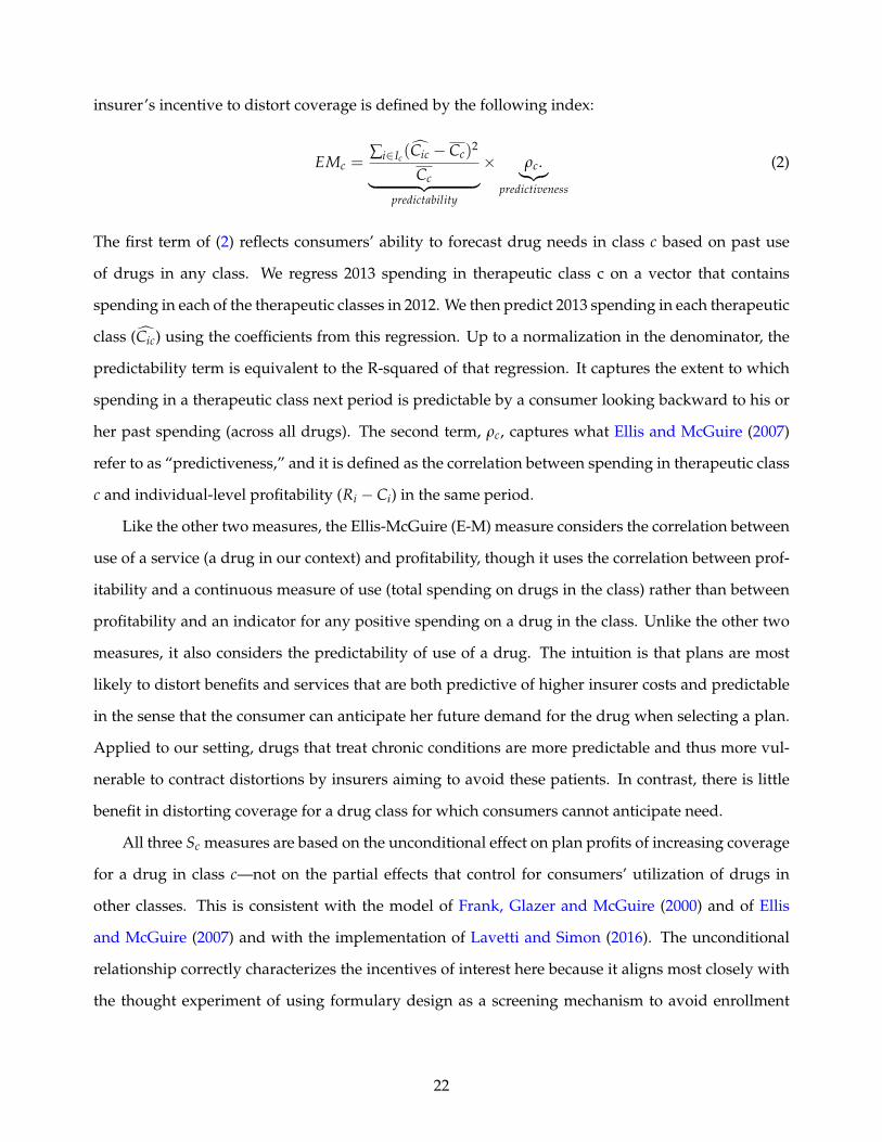
5.1 Selection Incentive Measures

We generate three alternative measures of the class-specific incentive, Sc, for Exchange plans to distort

coverage:

Sc =

Cc − Rc Cost-revenue difference,

Cc

RcCost-to-revenue ratio,

EMc Ellis-McGuire predictable profitability.

(1)

In all cases, higher positive values of Sc are associated with stronger incentives to inefficiently restrict

coverage for the class. The first two measures are self-explanatory. The third measure is based on

Ellis and McGuire (2007), which developed a theory of health plan benefit distortions in the presence

of adverse selection on service-level benefits. Ellis and McGuire (2007) show that a profit-maximizing

44The positive vertical movement of these points is small enough to be imperceptible in the figure.

21

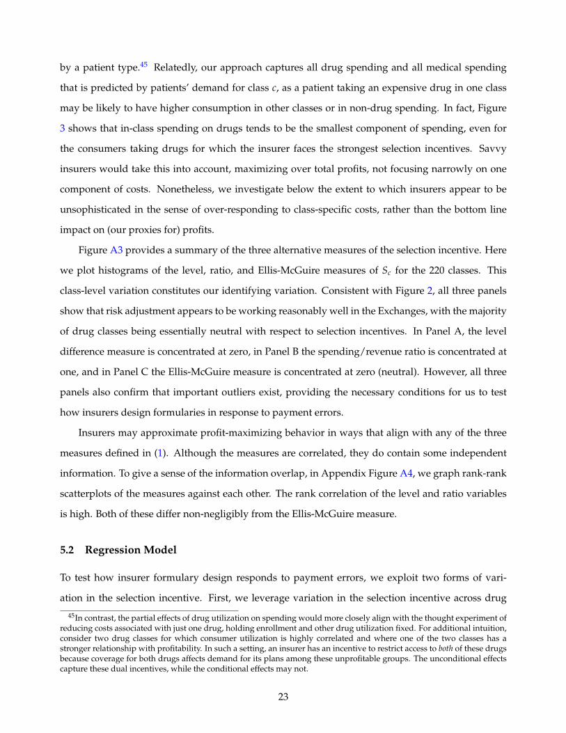
insurer’s incentive to distort coverage is defined by the following index:

EMc =∑i∈Ic

(Cic − Cc)2

Cc︸ ︷︷ ︸predictability

× ρc.︸︷︷︸predictiveness

(2)

The first term of (2) reflects consumers’ ability to forecast drug needs in class c based on past use

of drugs in any class. We regress 2013 spending in therapeutic class c on a vector that contains

spending in each of the therapeutic classes in 2012. We then predict 2013 spending in each therapeutic

class (Cic) using the coefficients from this regression. Up to a normalization in the denominator, the

predictability term is equivalent to the R-squared of that regression. It captures the extent to which

spending in a therapeutic class next period is predictable by a consumer looking backward to his or

her past spending (across all drugs). The second term, ρc, captures what Ellis and McGuire (2007)

refer to as “predictiveness,” and it is defined as the correlation between spending in therapeutic class

c and individual-level profitability (Ri − Ci) in the same period.

Like the other two measures, the Ellis-McGuire (E-M) measure considers the correlation between

use of a service (a drug in our context) and profitability, though it uses the correlation between prof-

itability and a continuous measure of use (total spending on drugs in the class) rather than between

profitability and an indicator for any positive spending on a drug in the class. Unlike the other two

measures, it also considers the predictability of use of a drug. The intuition is that plans are most

likely to distort benefits and services that are both predictive of higher insurer costs and predictable

in the sense that the consumer can anticipate her future demand for the drug when selecting a plan.

Applied to our setting, drugs that treat chronic conditions are more predictable and thus more vul-

nerable to contract distortions by insurers aiming to avoid these patients. In contrast, there is little

benefit in distorting coverage for a drug class for which consumers cannot anticipate need.

All three Sc measures are based on the unconditional effect on plan profits of increasing coverage

for a drug in class c—not on the partial effects that control for consumers’ utilization of drugs in

other classes. This is consistent with the model of Frank, Glazer and McGuire (2000) and of Ellis

and McGuire (2007) and with the implementation of Lavetti and Simon (2016). The unconditional

relationship correctly characterizes the incentives of interest here because it aligns most closely with

the thought experiment of using formulary design as a screening mechanism to avoid enrollment

22

by a patient type.45 Relatedly, our approach captures all drug spending and all medical spending

that is predicted by patients’ demand for class c, as a patient taking an expensive drug in one class

may be likely to have higher consumption in other classes or in non-drug spending. In fact, Figure

3 shows that in-class spending on drugs tends to be the smallest component of spending, even for

the consumers taking drugs for which the insurer faces the strongest selection incentives. Savvy

insurers would take this into account, maximizing over total profits, not focusing narrowly on one

component of costs. Nonetheless, we investigate below the extent to which insurers appear to be

unsophisticated in the sense of over-responding to class-specific costs, rather than the bottom line

impact on (our proxies for) profits.

Figure A3 provides a summary of the three alternative measures of the selection incentive. Here

we plot histograms of the level, ratio, and Ellis-McGuire measures of Sc for the 220 classes. This

class-level variation constitutes our identifying variation. Consistent with Figure 2, all three panels

show that risk adjustment appears to be working reasonably well in the Exchanges, with the majority

of drug classes being essentially neutral with respect to selection incentives. In Panel A, the level

difference measure is concentrated at zero, in Panel B the spending/revenue ratio is concentrated at

one, and in Panel C the Ellis-McGuire measure is concentrated at zero (neutral). However, all three

panels also confirm that important outliers exist, providing the necessary conditions for us to test

how insurers design formularies in response to payment errors.

Insurers may approximate profit-maximizing behavior in ways that align with any of the three

measures defined in (1). Although the measures are correlated, they do contain some independent

information. To give a sense of the information overlap, in Appendix Figure A4, we graph rank-rank

scatterplots of the measures against each other. The rank correlation of the level and ratio variables

is high. Both of these differ non-negligibly from the Ellis-McGuire measure.

5.2 Regression Model

To test how insurer formulary design responds to payment errors, we exploit two forms of vari-

ation in the selection incentive. First, we leverage variation in the selection incentive across drug

45In contrast, the partial effects of drug utilization on spending would more closely align with the thought experiment ofreducing costs associated with just one drug, holding enrollment and other drug utilization fixed. For additional intuition,consider two drug classes for which consumer utilization is highly correlated and where one of the two classes has astronger relationship with profitability. In such a setting, an insurer has an incentive to restrict access to both of these drugsbecause coverage for both drugs affects demand for its plans among these unprofitable groups. The unconditional effectscapture these dual incentives, while the conditional effects may not.

23

classes within a plan. Figure 2 shows the extent of this variation. Second, we leverage variation

in the selection incentive between the Exchange and employer-sponsored insurance markets. Ex-

change plans and employer-sponsored plans plausibly face similar considerations in balancing risk

protection against consumer moral hazard, in steering consumers to cost-effective options, and in

responding to other phenomena relevant for efficient benefit design. However, selection incentives

differ significantly in the two settings. Even if large, self-insured employers were able to significantly

influence their enrollee pool (and there are reasons to believe the scope for such behavior is small),

these employer plans do not face the Exchange risk adjustment and reinsurance payment scheme,

and so they do not face the screening incentives, Sc, that comprise the identifying variation here.46

Thus, we identify insurer formulary design responses to payment errors by comparing the difference

in formulary design for drug classes with strong selection incentives to classes with weak selection

incentives in Exchange plans to the same difference for self-insured employer plans.

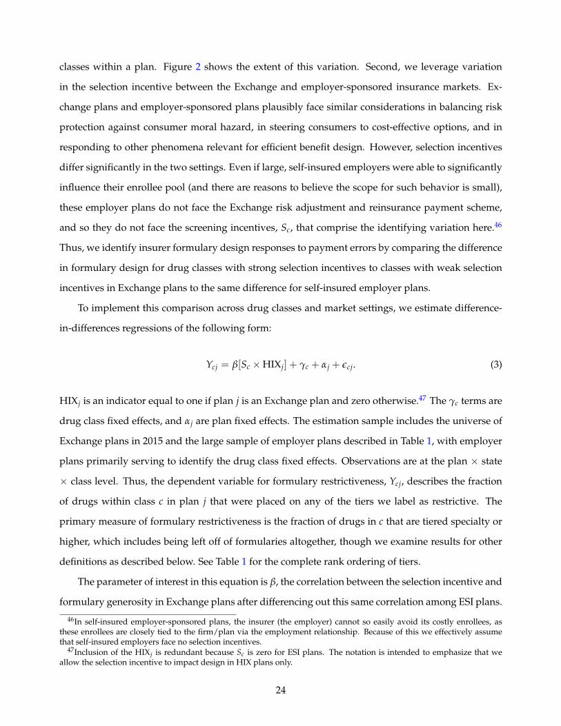
To implement this comparison across drug classes and market settings, we estimate difference-

in-differences regressions of the following form:

Ycj = β[Sc ×HIXj] + γc + αj + εcj. (3)

HIXj is an indicator equal to one if plan j is an Exchange plan and zero otherwise.47 The γc terms are

drug class fixed effects, and αj are plan fixed effects. The estimation sample includes the universe of

Exchange plans in 2015 and the large sample of employer plans described in Table 1, with employer

plans primarily serving to identify the drug class fixed effects. Observations are at the plan × state

× class level. Thus, the dependent variable for formulary restrictiveness, Ycj, describes the fraction

of drugs within class c in plan j that were placed on any of the tiers we label as restrictive. The

primary measure of formulary restrictiveness is the fraction of drugs in c that are tiered specialty or

higher, which includes being left off of formularies altogether, though we examine results for other

definitions as described below. See Table 1 for the complete rank ordering of tiers.

The parameter of interest in this equation is β, the correlation between the selection incentive and

formulary generosity in Exchange plans after differencing out this same correlation among ESI plans.

46In self-insured employer-sponsored plans, the insurer (the employer) cannot so easily avoid its costly enrollees, asthese enrollees are closely tied to the firm/plan via the employment relationship. Because of this we effectively assumethat self-insured employers face no selection incentives.

47Inclusion of the HIXj is redundant because Sc is zero for ESI plans. The notation is intended to emphasize that weallow the selection incentive to impact design in HIX plans only.

24

In most tables we present OLS estimates of (3), though we additionally present semi-parametric

versions in several figures. To facilitate interpretation of β, in all regressions we standardize Sc by

subtracting its mean and dividing by its standard deviation. This places results for the various op-

erationalizations of the selection incentive on a comparable (z-score) scale. Data are weighted by

covered lives within the plan, so that the estimates are representative of the Exchanges nationally for

2015. Standard errors are clustered at the level of the 220 drug classes.

5.3 Identification

The ESI population is a natural choice for a control group here. The MarketScan sample of ESI plans,

in particular, is what CMS chose to use when calibrating risk adjustment for the Exchanges, deter-

mining it to be the most comparable population for which claims data was available. Nonetheless,

identifying Exchange plans’ responses to the screening incentive does not require that Exchange and

employer plans are equally generous in practice or that they should be equally generous in terms of

socially optimal design. Plan fixed effects in Equation (3) address any differences in overall generos-

ity between Exchange and employer plans, so that β is identified by the differential slope∂Ycj

∂Scwithin

Exchange plans relative to within ESI plans. Our strategy also does not require that ESI benefits

arrangements achieve the social optimum. Instead, the key assumption is that the Exchange pay-

ment formula error, which differs across drug classes, is not correlated with some other drug class

characteristic that is relevant for formulary design and that differs for a given drug class between the

Exchange and employer markets. Under the assumption that Sc is orthogonal to other employer-

Exchange differences influencing formulary design, what we identify is whether Exchange insurers

are responsive to the financial incentives embedded in the Exchange payment errors. If one further

assumed that employer plan formularies are (approximately) optimal, then one could further inter-

pret the responsiveness of Exchange plans to the screening incentives as deviations away from the

optimal contract. Here, however, our intention is only to understand whether—and with what de-

gree of apparent sophistication—insurers respond to these incentives, not to characterize the optimal

contract.

To make the identifying assumption concrete, consider a case that would violate it. Assume

that the selection incentives in the Exchanges (Sc) were correlated with healthcare costs in employer

plans, so that the consumer types that were under-compensated by the Exchange payment scheme

25

were the same consumer types who were disproportionately expensive to care for when enrolled in

employer plans. (Empirically, this is not the case, as Panel B of Figure 2 shows that there is no cor-

relation between Sc and healthcare costs in employer plans, but the thought experiment highlights

the important assumptions.) One might imagine that employers with wage rigidities would wish to

discriminate against high medical-cost workers, as high cost types would drive up total compensa-

tion. These firms might use insurance design to help facilitate this employment discrimination. If this

were the case, our estimates would be biased. In this case, the bias would cause us to underestimate

the impact of the Exchange screening incentive, as would any phenomenon leading to correlation

between Sc in the Exchanges and reduced generosity for class c in the employer setting.

Another potentially relevant issue with respect to identification is whether Exchange and employer-

enrolled consumers differ in their price elasticities of demand for prescription drugs. They may. But

only differences across ESI and Exchange enrollees in class-specific demand elasticities that happened

to be correlated with the class-specific errors in the payment formula would violate our identifying

assumption. This seems unlikely a priori, especially given evidence presented in Section 7 that there

is no correlation between our measures of the screening incentives and a set of estimates for class-

specific demand elasticities from the Medicare Part D market.48

6 Effects on Formulary Designs

6.1 Main Results

We start by illustrating the basic correlations underlying our main results semi-parametrically. Fig-

ure 5 shows how the generosity of coverage differs between Exchange and ESI plans according to

the strength of the screening incentive associated with each drug class. Each of the three screening

incentive measures are presented. To create each figure, we regress formulary restrictiveness on drug

class fixed effects and plan fixed effects and compute the residuals. We then group therapeutic classes

c into ventiles according to the strength of each selection incentive measure Sc. The vertical axes in

each panel measure the means of the residuals within each ventile, separately for employer and Ex-

48A related idea is that Exchange plans may for some reason be more responsive to the same demand elasticities displayedby consumers in employer plans. We investigate this possibility directly, by examining the relationship between Sc andindependent estimates of drug class-specific price elasticities of demand from Einav, Finkelstein and Polyakova (2016).

26

change plans.49 In the plots on the left, the horizontal axes measure the mean of Sc within the bin, and

in the plots on the right, the horizontal axes are scaled by the ventile bin number (1-20). Residuals

corresponding to Exchange plans exhibit substantially more noise given the relatively small size of

the universe of Exchange plans (n = 501).50

Because risk adjustment succeeds in neutralizing selection incentives for most classes, many of

the scatterpoints in Panels A, C, and E of Figure 5 are clustered near neutral (Sc = 0) along the

horizontal axes. Where the incentives diverge from neutrality, so does benefit design. Formulary

restrictiveness is significantly different between employers and Exchanges at the highest ventiles (in

the rightmost bins), with the Exchange plans providing much less generous coverage for the drugs

that are signals of very unprofitable enrollees. For the drug classes where risk adjustment is predicted

to systematically overpay relative to costs (in the leftmost bins), Exchange formularies on average

provide relatively more generous coverage, though these differences are smaller than the differences

for the classes with the strongest incentives to screen out enrollees.

Table 3 presents regression results corresponding to Equation (3). We report the difference-in-

differences coefficient estimates for the interaction between the Exchange dummy and the selection

measure, HIXj × Sc. All regressions include plan and drug class fixed effects. The selection incentive

variable, Sc, varies across columns, as indicated in the column headers. In Panel A the dependent

variable is the fraction of drugs within the class placed on the specialty tier or higher. This corre-

sponds to the restrictive tier cutoff indicated in Table 1, and the measure used in Figure 5. In Panel

B the dependent variable is the fraction of drugs within the class that require prior authorization

or step therapy (PA/ST) or that are explicitly called out on the formulary as “not covered.” Given

the possibility of non-linear effects suggested by the residuals in Figure 5, we present both linear

specifications and specifications that allow the relationship to be non-linear at the top ventile.51

Table 3 shows that Exchange plans tend to provide less generous coverage (more frequent place-

ment on the specialty tier or higher) for drug classes where stronger selection incentives are generated

by the payment system. The interpretation of the coefficient in column (1) is that a one standard de-

viation increase in the strength of the selection incentive increases the class-specific drugs assigned

49Each ventile contains around 11 classes. The classes, in turn, contain many individual drugs, but analyses in the paperoperate at the level of classes, not at the level of individual drugs.

50Recall from Section 3 that the definition of an Exchange “plan” in this context aggregates various insurance productsoffered by the same carrier in the same market that share a common a formulary.

51These additionally include the regressor HIXj ×V20, where V20 is an indicator for the class having a selection incentivein the top 5% of the distribution of Sc.

27

to a restrictive tier by about 4.6 percentage points in Exchange plans relative to employer plans. This

is a substantial increase relative to a baseline restrictive tier use of 43% in employer plans and 59%

in Exchange plans. Coefficients across the linear specifications in Panel A are similar, regardless of

which of the three incentive measures is used as Sc. For the difference and Ellis-McGuire measures,

the non-linear specifications generate a better fit. The results in column (6) indicate that even control-

ling for a linear relationship between Sc and restrictiveness, drugs in the top ventile of the selection

incentive measures face an additional 69 percent (= .296.43 ) probability of being placed on a specialty

tier or higher.

One way to put these patterns in context is to consider the difference in formulary structure

associated with moving from the 90th percentile of profitability among therapeutic classes to the

10th percentile. Employer plan formularies, which are not subject to the Exchange payment scheme

generating Sc, don’t track this incentive: For employer plans the 90/10 selection incentive difference

is associated with going from 43% of drugs being placed on a restrictive tier to 45%. Among Exchange

plans, the same 90/10 difference is associated with an increase in restrictive tiering from 53% to

76%.52 To benchmark these effects, we note that the implied difference-in-differences, (76− 53) −

(45− 43) = 21, is a bit larger than the 16 percentage point gross difference in mean plan generosity

between Employer and Exchange plans shown in Table 1.

Although the vast majority of consumers will not fill prescriptions in the most unprofitable

classes, these differences can be economically sizable for the consumers affected. Recall that the

difference between a non-restrictive tier and a restrictive tier is generally associated with the change

from copay-based to coinsurance-based cost-sharing (or to no coverage at all). Drugs in unprofitable

classes like biological response modifiers can be priced in excess of $4,000 per month (Lotvin et al., 2014).

Thus, the out-of-pocket costs associated with even a 20% coinsurance rate would be an order of mag-

nitude larger than copay-based cost sharing and could routinely push such patients to their annual

out of pocket maximum.53 Such out of pocket costs are relevant not only for consumers who are

currently chronically ill; they also imply that currently healthy consumers cannot be adequately in-

sured against the negative shock of transitioning to one of the poorly-covered chronic disease states.

Additionally, these results suggest that if there were no risk adjustment in this market, dramatically

52These statistics are based on simple means within the sample, they are not derived from regression coefficients. Theratio measure is used to rank the classes by profitability here.

53In 2015 the out-of-pocket annual maximum could not exceed $6,600 for an individual Exchange plan and $13,200 for afamily plan, though plans were free to set lower limits.

28

increasing the screening incentives for many drug classes, many additional consumers would face

much higher out-of-pocket costs for their drugs.

In Panel B of Table 3, we investigate whether plans tailor more than just cost sharing amounts in

responding to Sc. One reason to do so might be the ACA’s cost sharing reduction subsidies (CSRs).

About half of Exchange enrollees during our time period were enrolled in a CSR variant of a Silver

plan. Importantly, CSR-eligible consumers enroll in nominally the same plans as non-CSR consumers

and face the same formulary structures. The CSR variants differ in that subsidies paid by the govern-

ment reduce the consumer’s out of pocket exposure and increase the actuarial value of the plan. (Ta-

ble 1 shows that copays at each formulary tier are smaller in CSR plans relative to the corresponding

“standard” Silver plan.) This feature limits insurers’ ability to rely on consumer cost sharing—either

as a potentially efficient response to moral hazard or as a socially inefficient screening tool. Perhaps

this is one reason why, as shown in Table 1, ten percent of all drugs in Exchange plans were subject

to prior authorization or step therapy, compared to less than one percent among employer plans.

Panel B Table 3 shows that this overall difference in utilization management varies by drug class

and is strongly correlated with patient profitability. Drugs in unprofitable classes are more likely to

not be covered or to face prior authorization or step therapy requirements. From column (7), a one

standard deviation increase in the strength of the selection incentive increases the percent of drugs

that are PA/ST or not covered by 1.8 percentage points on a base of 30%. Our findings for these

outcomes contrast with results from the Medicare part D setting, which find no positive relationship

between unprofitability and exclusion from the formulary.54 Our findings with respect to utilization

management and formulary inclusion provides a warning and counterpoint against policy reactions

to the discrimination/screening problem that would attempt to inhibit discriminatory behavior by

constraining plans’ ability to set cost sharing. Plans have many (potentially difficult to observe)

dimensions along which to increase the shadow price of accessing care.

For completeness, in Appendix Table A1, we report on a wider variety of non-linear specifi-

cations. In Appendix Figure A5, we plot semi-parametric versions of the regressions.55 Each of

54Lavetti and Simon (2016) find small, insignificant effects on utilization management and opposite-signed effects on theprobability that a drug is excluded from the formulary. Carey (2017a) finds no effect on the probability of exclusion fromthe formulary and does not examine impacts on the utilization management margins. Nonetheless, low income subsidyenrollees in Part D are similarly shielded from copays.

55Figure A5 plots binned means of the 220 regression coefficients βc from the regression Ycj = ∑c∈C βc × [Sc ×HIXj ×Ic] + γc + αj + εcj, where Y is the fraction of drugs assigned to a restrictive tier and Ic is an indicator for the class. Theclasses, c, are binned into ventiles of the strength of the screening incentive, Sc, and the means of β are plotted against themeans of Sc for each ventile.

29

these alternative specifications yields the same pattern of results. In all cases, tiering effects are large

and significant at the highest ventiles of the selection incentive, which contain the most unprofitable

enrollees. The special insight from the non-linear specifications is that effects do not appear to be

symmetric, as the magnitude and statistical significance of effects at the lowest ventiles (containing

the most profitable enrollees) are sensitive to specification.56 In summary, we find that Exchange

plans are designing their drug formularies to offer differentially worse coverage for classes used by

the most unprofitable individuals, consistent with the hypothesis that Exchange plan formularies are

designed as screening devices.

6.2 Insurer Sophistication

It could be the case that insurers are naively responding to the gross costs of potential enrollees and

not actually taking into account the fairly complex risk adjustment payments that determine net prof-

itability. However, Panel B of Figure 2 suggests that insurers must be at least somewhat sophisticated

in looking beyond costs, as there is no strong relationship between costs and profitability overall. In

other words, if insurers were attempting to screen out high cost enrollees without taking into account

risk adjustment and reinsurance payments, we would not observe the correlations we document in

Figure 5 between restrictiveness and profitability. In this section, we dig deeper into issues of insurer

sophistication.

Table 4 presents a series of “horserace” regressions testing whether formulary design more closely

tracks the expected costs or expected profits of potential enrollees. In Panel A we add to the main

regression specification controls for the average total healthcare spending associated with the ther-

apeutic class c, interacted with the Exchange indicator. In Panel B, we add controls for the average

spending on drugs, again interacted with the Exchange indicator. In Panel C, we include controls

for both average total healthcare spending associated with the class and average drug-only spend-

ing associated with the class. In the first three columns within each panel, we control linearly for

the interaction(s). One might think of the coefficients on these additional controls as measuring a

naive version of the selection incentive, in which risk adjustment and reinsurance are not taken into

account by Exchange plans, or in which the Exchange insurer is narrowly focused on the specific

56For the most theoretically-grounded measure of the selection incentive (Ellis-McGuire), the relationship is significantin both directions with positive coefficients for the top three ventiles (most unprofitable) and a negative coefficient on thebottom ventile (most profitable).

30

costs of the drugs, rather than on the broader signal of profitability implied by medication use. In the

second three columns, we flexibly control for the interaction with indicators for 20 bins of costs.57

Table 4 suggests that HIX insurers do in fact respond to gross total and drug-only costs in setting

formularies, but simultaneously respond to the expected profits. In columns (1) through (3) and (7)

through (9), coefficients on the controls for total and drug costs are statistically significant and in

the direction of more restrictive tiering for more expensive patients.58 This suggests that relative

to employer plans, Exchange plans develop formularies that are differentially less generous for the

drugs used by the more expensive enrollees. Nonetheless, the coefficients of interest (on HIXj × Sc)

are generally robust to the inclusion of these controls. In Appendix Table A2, we present a wider

array of specifications that flexibly control for costs in various ways, yielding very similar results.

Insurers thus appear to respond to net profitability in addition to, and independently from, gross

costs. The fact that there is any response to gross drug costs (relative to employer plans) is consistent

both with unsophisticated screening attempts or with the idea that insurers are attempting to cut

costs by offering poor coverage for whole classes of expensive drugs.

Although we have framed these results in terms of sophistication, another way to view the Table

4 and A2 regressions is as a robustness exercise. By estimating effects within sets of drug classes asso-

ciated with similar spending (essentially within narrow vertical slices of the scatterplot in Figure 2),

we rule out the possibility that the results are driven by a correlation between the selection incentive

and costs coupled with some differential response to costs in Exchange plans relative to employer

plans.59

Another way in which insurers may reveal sophistication is to specifically target drugs that will

be most salient in dissuading unprofitable consumers from joining at the time of plan enrollment.

In Panel A of Table 5 we investigate the possibility that popular drugs within each class are more

likely to be relegated to restrictive tiers in Exchange plans when under-compensated by the payment

system. In this table, we recalculate the dependent variable—the mean of the restrictive tier indicator

within the class—over just the most popular drugs in each class. To do so, we rank each drug within

57The specifications are otherwise identical to the linear specifications in Panel A of Table 3.58Simultaneously including drug and non-drug costs in Panel C yield less precise coefficients on these two cost controls

as they are correlated.59For example, if Exchange plans had an interest in placing a larger burden for expensive treatments on patients, and

if costs were correlated with Sc, we could mistake this behavior as screening. These specifications rule out this possi-bility. Another type of confounder ruled out is that demand elasticities that are differentially increasing in costs acrossthe employer and Exchange patient populations, and Exchange plans are merely responding to these demand elasticitydifferences.

31

each class according to the frequency of its consumption in the Marketscan data. We then calculate the

restrictive tiering variable for only those drugs lying above a cutoff percentile, where the percentiles

are weighted by consumption.60 Columns (1) through (6) of Table 5 present results for the 75th and

90th percentiles of popularity. At both thresholds, coefficients are larger when focusing on the most

popular drugs, compared to coefficients applying to the entire class from Table 3. When narrowly

focusing on the 90th percentile of popular drugs within each class, the coefficient sizes approach twice

the size of the main results. Thus, Exchange plans seem to limit coverage for popular drugs used by

unprofitable enrollees more than they do for less popular drugs, though it is unclear whether this

reflects insurers responding to salience of these drugs for consumers, or reflects insurers themselves

displaying a salience bias towards these drugs in formulary design.

All of this evidence is consistent with insurers designing their formularies to screen out unprof-

itable enrollees. We note that an important input to the theory connecting screening incentives to

formulary design is plan demand response of unprofitable consumers to drug coverage. We do not

provide direct evidence of this type of relationship between demand, unprofitability, and formulary

design. Indeed, this would be difficult to do in the Exchange setting as there is no available plan-level

enrollment data linkable to patient health conditions and utilization.61 Instead, we interpret our re-

sults as indirect evidence of the phenomenon described in Section 2. We also interpret the salience

results described in Table 5 as further evidence for this relationship, given that the effects are stronger

for the more popular drugs in each class.

Additionally, the related literature has shown in other contexts a clear relationship between drug

coverage and demand for a given insurance plan. In the context of Medicare Part D, Heiss et al.

(2013) show that plan demand in year t + 1 is responsive, albeit imperfectly, to the implied cost shar-

ing of that plan for the individuals’ year t prescriptions. Han and Lavetti (2017) provide evidence that

60For example, to compute the 75th percentile of popularity for a class in which one drug comprises 30% of the con-sumption share and seven other drugs each comprise 10% shares, the dependent variable would be computed only for thesingle drug with the 30% share.

61Even if such data were available, and even if consumers’ plan demand was responsive to formulary design, the properempirical test is not obvious: In a partial equilibrium sense, plans with more generous benefits for unprofitable typesshould attract them. But it may be the case that in general equilibrium, no plan will wish to offer such benefits, as deviationsfrom that skimpy-coverage strategy would be unprofitable. The question hinges on the nature of the equilibrium and inparticular whether a separating equilibrium (by drug class enrollee type) exists in practice. For example, Frank, Glazerand McGuire (2000) consider a symmetric equilibrium in which all plans offer poor coverage for services demanded byunprofitable types. In that model, there is no net sorting of consumer types across plans. The only common predictionacross the models in this literature (Rothschild and Stiglitz, 1976; Frank, Glazer and McGuire, 2000; Glazer and McGuire,2000; Veiga and Weyl, 2016; Azevedo and Gottlieb, 2017) is a reduction in the average generosity of coverage for servicesthat predict unprofitable patients. This is the empirical test Tables 3 and 4 implement.

32

enrollment decisions on the Traditional Medicare/Medicare Advantage (MA) margin respond to for-

mulary designs in MA-Part D plans. Of course, consumers may underweight the out-of-pocket costs

implied by formularies relative to premiums (Abaluck and Gruber, 2011) and may exhibit significant

inertia (Ho, Hogan and Scott Morton, 2017; Carey, 2017b), but even weak consumer responsiveness

may make it worthwhile for insurers to be attentive to screening considerations in benefit design.62

7 Discrimination or Efficient Design?

In this section, we provide evidence that our results cannot be rationalized by differential responses

of Exchange plans to the availability of cost effective substitutes within therapeutic classes or to dif-

ferences in consumer price sensitivity across classes. We also show that the results are not driven by

different pharmacy benefit managers across employer and Exchange markets. We focus here on dif-

ferential responses of Exchange and employer plans because the inclusion of drug class fixed effects

in our main analysis already controls for any similar response to these considerations across the two

markets.

7.1 Substitution to Cheaper Drugs and Generics

Insurers have a cost-saving interest in steering consumers to less expensive medications among al-

ternatives with similar efficacy. This behavior is also likely to be socially efficient. Therefore, one

potential explanation for our findings is that Exchange plans simply have a stronger interest than ESI

plans in operating at the efficient frontier and therefore do a better job of steering patients to lower-

cost alternatives within a class. There are two reasons that this is unlikely to explain our results. First,

such an explanation would be difficult to motivate under a model in which employers providing ESI

are profit maximizing. Such firms would have strong incentives to design an efficient health plan, al-

lowing them to compensate workers with higher wages (Bhattacharya and Bundorf, 2009).63 Second,

there is no a priori reason why, even if steering incentives were stronger in the Exchanges overall, HIX

plans’ interest in steering would be differentially strong across classes in a way that is correlated with62Regardless of the actual consumer plan demand elasticity with respect to formulary design, one could interpret the

results here as revealing that plans believe consumers will be somewhat responsive to the cost sharing. For example,consistent with such beliefs, Aetna launched Marketplace plans for 2016 that were specifically marketed toward diabetics.In these plans, Aetna set low cost sharing for specialist visits linked to diabetes management in an apparent effort to attractdiabetics Andrews (2015).

63The alternative would be to offer an inefficient plan that generated the same utility at a higher cost, leading to lowerwages, or to offer a plan at the same cost that generated lower utility.

33

the error in the HHS risk adjustment and reinsurance scheme. Nonetheless, we can provide some

direct evidence that efforts by Exchange insurers to incentivize efficient substitution are not driving

our results.64

To begin, we note that many of the drugs in classes with the strongest selection incentives have

no generic equivalents. For example, the entire class of Biologic Response Modifiers contains not a

single generic. In Appendix Table A6, we show that our results hold if we limit attention to classes

without generics (28 classes), with less than 10% generics (49 classes), or with less than 25% generics

(84 classes). Thus, our results cannot be driven by HIX plans using stronger nudges towards generics,

as the results hold in the absence of a generic alternative.

We also show in Appendix Table A5 that our qualitative patterns hold if we look just within the

generic drugs of a class or just within the branded drugs of a class. Using the same specification

as in the main results (Table 3) but including only generic drugs when measuring the formulary

restrictiveness, we show in Panel B of Table A5 that the selection incentive significantly predicts

restricted access to generics. The way tiers are harmonized across the diverse formularies of our data

does not mechanically allow for generics to be allocated to the specialty tier, so this result comes from

HIX plans using non-price hurdles to restrict access to generics. This is consistent with supplemental

summary statistics we present in Table A3, which show that HIX plans are ten times more likely than

employer plans to require prior authorization or step therapy for a generic, and are about twice as

likely to not cover a generic on their formulary. For completeness, we also show that additionally

controlling for the fraction of generic drugs within each class interacted with HIX does not alter

results (Table A7).

Encouraging substitution toward lower cost alternatives may occur along other margins than

brand versus generic. To investigate this possibility, in columns (7) through (12) of Table 5, we repeat

the main analysis but restrict attention to just the cheapest (generic and branded) drugs within each

class, as observed in the Marketscan data. This specification focuses on only the low-cost potential

substitutes in each class. Table 5 shows that the results hold up to examining the tiering of only

the least expensive 25% or 10% of drugs in each class. Coefficients are similar to the main results,

indicating that even relatively cheap drugs that are associated with expensive patients are placed on

64One possibility that we can not directly address in these data is that intertemporal spending spillovers (Fang andGavazza, 2011) may be internalized differently in ESI versus HIX plans, due to different rates of enrollee turnover. Thiscould cause drug coverage to differ across plan types. This would pose a problem only if such drug-class-specific dynamicincentives correlated with the error in the HHS risk adjustment and reinsurance scheme.

34

high cost sharing tiers. Taken together, Tables 5, A3, A5, A6, and A7 support the idea that the contract

designs we document do not merely reflect HIX plans pushing consumers to lower cost alternatives.

7.2 Demand Elasticity

As we highlight in Section 2, moral hazard, reflected in demand elasticities, is a key consideration in

a profit maximizing insurer’s formulary design problem (Einav, Finkelstein and Polyakova, 2016). It

is also an important component of the design of a socially-efficient health insurance contract (Glazer,

Huskamp and McGuire, 2012). The class fixed effects in our regressions are intended to control for

any class characteristics that are similar across ESI and Exchange settings, including own and cross-

price elasticities. However, a problem for identification could arise if ESI plans were differentially

responsive to the same consumer price elasticities, and if these class-specific price elasticities hap-

pened to be correlated with class-specific payment errors.

With this in mind, we explore sensitivity to excluding fertility-related classes. Table 2 showed

that two of the ten classes associated with the least profitable patients were associated with infertility,

a class for which one might expect especially high price sensitivity. We re-estimate our main regres-

sions excluding all fertility treatment classes in Appendix Table A8. The coefficients of interest are

almost numerically identical to our main results.

We also import external measures of class-specific demand elasticities estimated by Einav, Finkel-

stein and Polyakova (2016), who identify price sensitivity of prescription drug utilization by exploit-

ing Medicare Part D’s “donut hole” at which drug cost-sharing changes abruptly. Appendix Figure

A6 graphs scatterplots of these elasticities versus the strength of the selection incentive, revealing

that there is no significant correlation between Sc and consumer price sensitivity across classes. We

describe this exercise in detail in Appendix Section D, where we also show that our main results are

robust to directly controlling for class-specific demand elasticities in our regressions.

7.3 Contracting and Institutional Knowledge

Another possible explanation for our results is that the prices paid by insurers to drug manufacturers

differ between Exchange plans and employer plans due to differences in plans’ contracting with

manufacturers.65 To address this possibility to the extent possible in our data, we exploit the fact

65If upstream prices differ, then both profit-maximizing and (second-best) optimal consumer prices reflected in tiers,may also differ, following the intuition of Section 2.

35

that essentially all insurers outsource price negotiations with drug manufacturers to a fairly small

set of pharmacy benefit managers (PBMs). PBMs design the formularies, contract with pharmacies,

and negotiate prices. In our data, we observe the PBM used by each plan, allowing us to construct

a full set of PBM fixed effects. Let 1(PBMp) be an indicator equal to 1 if plan j uses PBM p and zero

otherwise. We estimate a set of specifications where we interact the selection incentive with the PBM

fixed effects (1(PBMp)× Sc) when estimating our coefficient of interest (β):66

Ycj = β[Sc ×HIXj] + ∑p

νp[1(PBMp)× Sc] + γc + αj + εcj (4)

Under this specification, β is identified off of differences between Exchange plans and employer plans

that use the same pharmacy benefit manager.

Table A9 displays these results, again separately for each selection measure. We present two

versions. In columns (1) through (4), we estimate Equation (4) such that the PBMp variable is de-

fined nationally. This implicitly compares, for example, Aetna’s Exchange plans in New Jersey to

Aetna’s employer plans in New Jersey and elsewhere. In columns (5) through (8), we control for

PBM-by-state fixed effects, so that the control is defined as [1(PBMp) × states × Sc]. Intuitively, in

these specifications we are comparing reactions to the selection incentive in, for example, employer

plans in Texas that contract with OptumRx (a PBM associated with United) to Exchange plans in

Texas that contract with OptumRx. In all cases the results in Table A9 are robust to these controls,

lending further support to our identifying assumption. These regressions address not only the bar-

gaining power confounder, but provide additional evidence that the effect is not driven by different

responses to (or different biased subjective beliefs about) consumer moral hazard across different

plan benefits architects.

8 Reinsurance Counterfactual

In 2017, the reinsurance program that had operated during the first three years of the Exchanges’

existence ended.67 In Section 4, we discuss how insurer screening incentives change with the removal

of the reinsurance program, holding all else fixed. Intuitively, reinsurance absorbs some part of the

66PBM main effects are absorbed by plan fixed effects.67As described in detail in Section 2.2, the ACA’s mandatory reinsurance program paid plans for outlying individual

enrollees with high realized spending.

36

under-payment errors that risk adjustment leaves behind, so its removal makes incentives worse for

the expensive classes that were already associated with unprofitable consumer types. In this section,

we simulate how insurers might be expected to alter their formularies in response to the removal of

reinsurance. We proceed with an important caveat. Because insurers were possibly learning about

their enrollee pools, costs, and profits over time in the first years of these new markets, because

there was significant policy uncertainty regarding the regulatory and payment system rules for the

Exchanges in 2017, and because these markets were in apparent disequilibrium in 2017, with insurers

exiting markets in several states, we present these counterfactuals not as predictions for 2017, but as

an alternative approach to providing intuition for the magnitudes of the screening phenomenon.

Table 6 shows how predicted restrictiveness differs with and without reinsurance. To compute

these measures we use the empirical models estimated in the odd columns of Table 3. The “with

reinsurance” columns in Table 6 simply generate predicted values from the regressions, using the

same measures of the screening incentive Sc used to estimate the model. For the “without reinsur-

ance” columns, we re-calculated the screening incentives to not include reinsurance payments or fees

(see Figure 4), and used these alternative values of Sc along with the original coefficient estimates to

generate predictions.68 In Panel A, we take the mean across all drug classes to produce the overall

average predicted percent of drugs on a restrictive tier. In Panel B, we describe the distribution of

changes in formulary generosity under the counterfactual. Percentiles in Panel B are at the level of

the drug class, with classes ordered according to the change in the fraction of drugs in the class pre-

dicted to be on the restrictive tier moving from a payment system with reinsurance to one without it.

Positive values in Panel B indicate more drugs on a restrictive tier under the no-reinsurance policy

regime.

The results reported in Panel A of Table 6 suggest that the counterfactual removal of reinsurance

in the 2015 markets would lead to an average increase in the percent of drugs on a restrictive tier of

around 2.5 percentage points and an average increase in the percent of drugs either excluded from

the formulary entirely or with prior authorization or step therapy requirements of a little over 1 per-

centage point. This is true despite it being the case that for some therapeutic classes, the removal

of (budget neutral) reinsurance reduces the overpayment, and brings the class closer to neutrality

68Consistent with the actual functioning of the Exchanges, we do not alter the risk adjustment algorithm when removingreinsurance. Parameters for these payment mechanisms were set independently, despite that optimization requires settingthem jointly (Layton and McGuire, 2017).

37

(the 45 degree line in Figure 4). To put these effects of reinsurance in context, recall from Table 1

that for Exchange plans around 59% of drugs appear on a restrictive tier while for employer plans

around 43% of drugs appear on a restrictive tier, a difference of 16 percentage points, implying that

reinsurance accounts for a sizeable portion of the difference between ESI and Exchange formulary

restrictiveness. The results in Panel B of Table 6 suggest that the small overall mean difference masks

significant heterogeneity. Classes at the 95th percentile of the distribution of changes experience

increases in restrictiveness between 6 and 10 percentage points and classes at the 99th percentile

experience increases in restrictiveness between 15 and 70 percentage points. These changes repre-

sent significant shifts in access to the associated drugs for Exchange plan enrollees, suggesting that

reinsurance plays an important role in the ACA plan payment system’s ability to maintain access to

drugs for some groups of enrollees, given the current risk adjustment system.

9 Discussion

We find that the ACA’s risk adjustment and reinsurance transfer payments are successful in neutral-

izing selection incentives for most, but not all, consumer types. Where payment errors exist, plans

offer poor coverage for the medications demanded by the corresponding patients. The distortions

we document currently affect a relatively small number of consumers, because only a small set of

consumer types are unprofitable, net of the ACA’s payment adjustments.69 Our findings show that

insurers are responsive to complex screening incentives where they exist, implying that it is only a

well-functioning risk adjustment and reinsurance system that keeps market forces from eroding ac-

cess to care for all costly patients. Further, the cost of these contract distortions is not solely borne by

patients currently burdened by the targeted chronic conditions. While that is an important and poten-

tially sizable distributional consequence, a welfare loss arises because in equilibrium consumers can-

not be adequately insured against the negative shock of transitioning to the poorly-covered chronic

disease state.70 This lack of risk protection can affect the utility of all consumers.

These results bear directly on a top concern among American consumers—high out-of-pocket

prices for prescription drugs. High consumer prices are almost always assumed to be caused by

upstream manufacturer prices. Our results confirm a clear, but often ignored, theoretical prediction:

69Some previous literature has also found the overall consequences of adverse selection to be small (Cardon and Hendel,2001).

70This transition risk parallels the premium reclassification risk discussed by Handel, Hendel and Whinston (2015).

38

It is unprofitable patients rather than expensive patients (or patients that use expensive drugs) who

are likely to bear high out-of-pocket costs. If the payment system were to generously compensate

insurers who enrolled patients consuming expensive drugs, then in equilibrium, such patients could

bear low out-of-pocket costs regardless of upstream drug prices.71

Our results also bear on the use of essential health benefits (EHB) rules as a means of guaran-

teeing healthcare access for certain services or patient types.72 The ACA’s EHBs mandate cover-

age of items and services in ten benefit categories, including prescription drugs. However, we find

that even while complying with these coverage mandates, plans design formularies that are signifi-

cantly unfavorable to consumer types that are unprofitable.73 Our findings thus suggest that simply

“strengthening” the list of mandated benefits, such as by mimicking Medicare Part D’s protected

class regulations, will not solve the problems documented here.74 Plans have many tools at their

disposal to limit coverage because their products are highly multidimensional. For example, if reg-

ulators restricted insurers’ flexibility in setting cost-sharing—a popular proposal in the context of

high patient drug costs—then plans could respond by relying more heavily on non-price barriers to

access, such as step-therapy and prior authorization. If regulators then restricted the use of tools

like prior authorization, plans could generate hurdles that were effectively invisible to the regulator,

such as requiring consumers to use in-house mail-order pharmacies for particular drugs and making

it difficult to work with those pharmacies. As a corollary, our findings suggest that weakening or

eliminating minimum coverage requirements, which has been proposed in various Republican plans

to repeal and replace the ACA, need not expose chronically-ill consumers to significant financial risk.

But this is true only if strong selection-related regulations, including risk adjustment and possibly

reinsurance, are in place.75

One possibility to address the distortions documented here is to refine the risk adjustment system

to directly incorporate limited drug utilization information, including possibly interactions between

71Upstream prices would nonetheless be important in determining premiums, but their effect on the financial risk asso-ciated with transitioning to a health state that requires a particularly expensive treatment would be less extreme.

72Setting aside questions of efficacy in combatting selection, excessive minimum coverage requirements can have thenegative welfare consequence of limiting the insurer’s ability to set coverage that trades off risk protection and moralhazard, which is a welfare-relevant tension in socially optimal insurance design (Pauly, 1968, 1974; Zeckhauser, 1970).

73See Andersen (2017) for further description and for evidence that the number of drugs covered is affected by the EHBs.74Medicare Part D requires plans to cover a minimum of two drugs per USP class and designates six protected classes

for which plans are required to cover all drugs.75See Layton and McGuire (2017) for a discussion of how risk adjustment and reinsurance in the Exchanges may be

modified within the current regulatory framework to generate payments that better match person-level costs for outlierenrollees.

39

drug utilization and medical diagnoses. HHS has suggested that by 2018, it will amend the risk ad-

justment algorithm used in the individual market in this way (Centers for Medicare and Medicaid

Services, 2016). Incorporating drug utilization into the risk adjustment system would be novel in

the US at the national level. Given experience with diagnosis-based risk adjustment, any such re-

form should be conducted with careful attention to impacts on administrative burden, impacts on

cost-control incentives, and the potential for gaming by insurers, which has been shown to be an

empirically relevant phenomenon (Geruso and Layton, 2015).76 Nonetheless, because drug utiliza-

tion actually requires real-world action by a patient at a pharmacy, rather than merely a paperwork

edit by a physician’s billing staff or by an insurer, it is possible that for some drug-class × diagnosis

interactions, gaming may be more difficult than it is under current diagnosis-only risk adjustment.

The US Medicare and Medicaid programs, the US individual and small group markets, and the

national health insurance programs of many members of the OECD have all come to increasingly

rely on private insurance carriers to design and manage publicly funded or subsidized health bene-

fits. Our results demonstrate that in such settings, ensuring non-discrimination requires more than

prohibiting overt discrimination and mandating minimum essential health benefits. It requires get-

ting the plan payment incentives right. Therefore, despite the inherent imperfections in using risk

scores to govern transfer payments across plans with different features and cost structures (Einav

et al., 2016), despite risk adjustment’s distortionary incentives to code patients intensely (Geruso

and Layton, 2015), and despite risk adjustment’s weakened incentives to restrain overall healthcare

spending relative to pure capitation (Geruso and McGuire, 2016), risk adjustment and reinsurance

play a crucial role in mitigating screening and selection problems endemic to competitive insurance

markets.

76Geruso and Layton (2015) show that patients’ reported diagnoses are endogenous to the plan in which they are enrolledin the context of Medicare Advantage. Drug utilization may be similarly endogenous.

40

References

Abaluck, Jason, and Jonathan Gruber. 2011. “Choice Inconsistencies among the Elderly: Evidencefrom Plan Choice in the Medicare Part D Program.” American Economic Review, 101(4): 1180–1210.

Aizawa, Naoki, and You Suk Kim. 2015. “Advertising and Risk Selection in Health Insurance Mar-kets.” Working Paper.

Akerlof, George A. 1970. “The Market for “Lemons”: Quality Uncertainty and the Market Mecha-nism.” Quarterly Journal of Economics, 84(3): 488–500.

Andersen, Martin. 2017. “Constraints on Formulary Design Under the Affordable Care Act.” HealthEconomics, Forthcoming.

Andrews, Michelle. 2015. “New Health Plans Offer Discounts for Diabetes Care.” Kaiser Health News.

Azevedo, Eduardo, and Daniel Gottlieb. 2017. “Perfect Competition in Markets with Adverse Selec-tion.” Econometrica, 85(1): 67–105.

Bhattacharya, Jay, and M. Kate Bundorf. 2009. “The Incidence of the Healthcare Costs of Obesity.”Journal of Health Economics, 28(3): 649–658.

Breyer, Friedrich, M. Kate Bundorf, and Mark V. Pauly. 2011. “Health Care Spending Risk, HealthInsurance, and Payment to Health Plans.” In Handbook of Health Economics. Vol. 2, , ed. Mark V.Pauly, Thomas G. McGuire and Pedro P. Barros, 691–762. Elsevier.

Brown, Jason, Mark Duggan, Ilyana Kuziemko, and William Woolston. 2014. “How Does Risk Se-lection Respond to Risk Adjustment? Evidence from the Medicare Advantage Program.” AmericanEconomic Review, 104(10): 3335–3364.

Cardon, James H., and Igal Hendel. 2001. “Asymmetric Information in Health Insurance: Evidencefrom the National Medical Expenditure Survey.” The RAND Journal of Economics, 32(3): 408–427.

Carey, Colleen. 2017a. “Technological Change and Risk Adjustment: Benefit Design Incentives inMedicare Part D.” American Economic Journal: Economic Policy, 9(1): 38–73.

Carey, Colleen. 2017b. “A Time to Harvest: Evidence on Consumer Choice Frictions from a PaymentRevision in Medicare Part D.” Working Paper.

Centers for Medicare and Medicaid Services. 2015. “Summary Report on Transitional ReinsurancePayments and Permanent Risk Adjustment Transfers for the 2014 Benefit Year.” Department ofHealth and Human Services.

Centers for Medicare and Medicaid Services. 2016. “March 31, 2016, HHS-Operated Risk Adjust-ment Methodology Meeting Discussion Paper.” Department of Health and Human Services.

Chandra, Amitabh, Jonathan Gruber, and Robin McKnight. 2010. “Patient Cost-sharing and Hos-pitalization Offsets in the Elderly.” American Economic Review, 100(1): 193–213.

Clemens, Jeffrey, Joshua D. Gottlieb, and Tímea Laura Molnár. 2017. “Do Health Insurers Innovate?Evidence from the Anatomy of Physician Payments.” Journal of Health Economics, 55(1): 153–167.

Decarolis, Francesco, and Andrea Guglielmo. 2017. “Insurers’ Response to Selection Risk: Evidencefrom Medicare Enrollment Reforms.” Journal of Health Economics, Forthcoming.

41

DeLeire, Thomas, Andre Chappel, Kenneth Finegold, and Emily Gee. 2017. “Do Individuals Re-spond to Cost-Sharing Subsidies in their Selections of Marketplace Health Insurance Plans?” Jour-nal of Health Economics, Forthcoming.

Einav, Liran, Amy Finkelstein, and Maria Polyakova. 2016. “Private Provision of Social Insurance:Drug-specific Price Elasticities and Cost Sharing in Medicare Part D.” National Bureau of EconomicResearch Working Paper 22277.

Einav, Liran, Amy Finkelstein, and Mark R. Cullen. 2010. “Estimating Welfare in Insurance MarketsUsing Variation in Prices.” Quarterly Journal of Economics, 125(3): 877–921.

Einav, Liran, Amy Finkelstein, Raymond Kluender, and Paul Schrimpf. 2016. “Beyond Statistics:The Economic Content of Risk Scores.” American Economic Journal: Applied Economics, 8(2): 195–224.

Ellis, Randall P., and Thomas G. McGuire. 2007. “Predictability and Predictiveness in Health CareSpending.” Journal of Health Economics, 26(1): 25–48.

Fang, Hanming, and Alessandro Gavazza. 2011. “Dynamic inefficiencies in an employment-basedhealth insurance system: Theory and evidence.” American Economic Review, 101(7): 3047–77.

Feldstein, Martin. 1973. “The Welfare Loss of Excess Health Insurance.” Journal of Political Economy,81(2): 251–280.

Frank, Richard G., Jacob Glazer, and Thomas G. McGuire. 2000. “Measuring Adverse Selection inManaged Health Care.” Journal of Health Economics, 19(6): 829–854.

Geruso, Michael, and Thomas G. McGuire. 2016. “Tradeoffs in the Design of Health Plan PaymentSystems: Fit, Power and Balance.” Journal of Health Economics, 47(1): 1–19.

Geruso, Michael, and Timothy J. Layton. 2017. “Selection in Health Insurance Markets and Its PolicyRemedies.” Journal of Economic Perspectives, Forthcoming.

Geruso, Michael, and Timothy Layton. 2015. “Upcoding: Evidence from Medicare on Squishy RiskAdjustment.” National Bureau of Economic Research Working Paper 21222.

Glazer, Jacob, and Thomas G. McGuire. 2000. “Optimal Risk Adjustment in Markets with AdverseSelection: An Application to Managed Care.” American Economic Review, 90(4): 1055–1071.

Glazer, Jacob, Haiden A Huskamp, and Thomas G McGuire. 2012. “A Prescription for Drug Formu-lary Evaluation: An Application of Price Indexes.” Forum for Health Economics & Policy, 15(2): 1558–95.

Hackmann, Martin B., Jonathan T. Kolstad, and Amanda E. Kowalski. 2015. “Adverse Selection andan Individual Mandate: When Theory Meets Practice.” American Economic Review, 105(3): 1030–1066.

Handel, Benjamin R., Igal Hendel, and Michael D. Whinston. 2015. “Equilibria in Health Ex-changes: Adverse Selection vs. Reclassification Risk.” Econometrica, 83(4): 1261–1313.

Han, Tony, and Kurt Lavetti. 2017. “Does Part D Abet Advantageous Selection in Medicare Advan-tage?” Journal of Health Economics, Forthcoming.

Heiss, Florian, Adam Leive, Daniel McFadden, and Joachim Winter. 2013. “Plan selection in Medi-care Part D: Evidence from administrative data.” Journal of Health Economics, 32(6): 1325–1344.

42

Ho, Kate, Joseph Hogan, and Fiona Scott Morton. 2017. “The Impact of Consumer Inattention onInsurer Pricing in the Medicare Part D Program.”

Jacobs, Douglas B., and Benjamin D. Sommers. 2015. “Using Drugs to Discriminate? Adverse Se-lection in the Insurance Marketplace.” New England Journal of Medicine, 372(5): 399–402.

Kautter, John, Gregory C. Pope, Melvin Ingber, Sara Freeman, Lindsey Patterson, Michael Co-hen, and Patricia Keenan. 2014. “The HHS-HCC Risk Adjustment Model for Individual and SmallGroup Markets under the Affordable Care Act.” Medicare & Medicaid Research Review, 4(3): E1–E46.

Kuziemko, Ilyana, Katherine Meckel, and Maya Rossin-Slater. 2013. “Do Insurers Risk-SelectAgainst Each Other? Evidence from Medicaid and Implications for Health Reform".” NationalBureau of Economic Research Working Paper 19198.

Lavetti, Kurt, and Kosali Simon. 2016. “Strategic Formulary Design in Medicare Part D Plans.” Na-tional Bureau of Economic Research Working Paper 22338.

Layton, Timothy J, and Thomas G McGuire. 2017. “Marketplace plan payment options for dealingwith high-cost enrollees.” American Journal of Health Economics, 3(2): 165–191.

Layton, Timothy J., Randall P. Ellis, Thomas G. McGuire, and Richard Van Kleef. 2017. “MeasuringEfficiency of Health Plan Payment Systems in Managed Competition Health Insurance Markets.”Journal of Health Economics, Forthcoming.

Lotvin, Alan M., William H. Shrank, Surya C. Singh, Benjamin P. Falit, and Troyen A. Brennan.2014. “Specialty Medications: Traditional and Novel Tools Can Address Rising Spending on TheseCostly Drugs.” Health Affairs, 33(10): 1736–1744.

Pauly, Mark V. 1968. “The Economics of Moral Hazard: Comment.” American Economic Review,58(3): 531–537.

Pauly, Mark V. 1974. “Overinsurance and Public Provision of Insurance: The Roles of Moral Hazardand Adverse Selection.” Quarterly Journal of Economics, 88(1): 44–62.

Rothschild, Michael, and Joseph Stiglitz. 1976. “Equilibrium in Competitive Insurance Markets: AnEssay on the Economics of Imperfect Information.” Quarterly Journal of Economics, 90(4): 629–649.

Shepard, Mark. 2016. “Hospital Network Competition and Adverse Selection: Evidence from theMassachusetts Health Insurance Exchange.” National Bureau of Economic Research Working Pa-per 22600.

Simon, Kosali, Sharon Tennyson, and Julie Hudman. 2009. “Do State Cost Control Policies ReduceMedicaid Prescription Drug Spending?” Risk Management and Insurance Review, 12(1): 39–66.

Starc, Amanda, and Robert J. Town. 2015. “Internalizing Behavioral Externalities: Benefit Integrationin Health Insurance.” National Bureau of Economic Research Working Paper 21783.

van de Ven, Wynand P. M. M., and Randall P. Ellis. 2000. “Risk Adjustment in Competitive HealthPlan Markets.” In Handbook of Health Economics. Vol. 1A, , ed. Anthony J. Culyer and Joseph P.Newhouse, 755–845. Elsevier.

Veiga, André, and E. Glen Weyl. 2016. “Product Design in Selection Markets.” Quarterly Journal ofEconomics, 131(2): 1007–1056.

Zeckhauser, Richard. 1970. “Medical Insurance: A Case Study of the Tradeoff Between Risk Spread-ing and Appropriate Incentives.” Journal of Economic Theory, 2(1): 10–26.

43

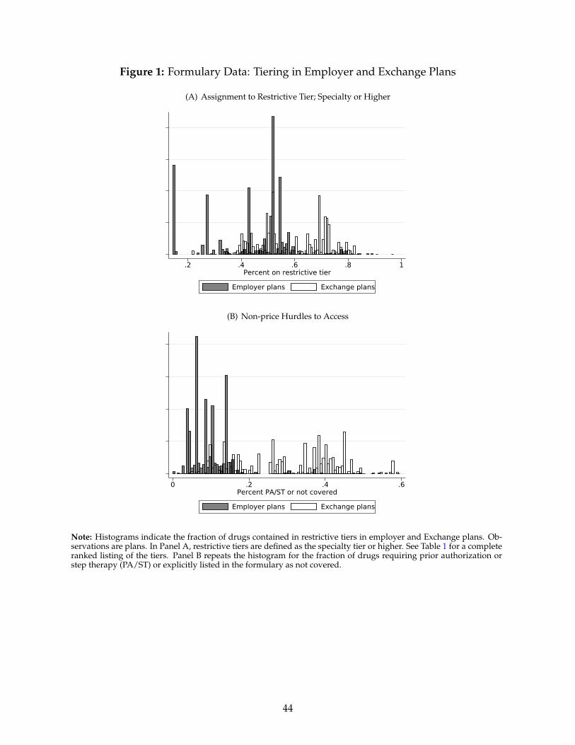
Figure 1: Formulary Data: Tiering in Employer and Exchange Plans

(A) Assignment to Restrictive Tier; Specialty or Higher

05

1015

20Pe

rcen

t

.2 .4 .6 .8 1Percent on restrictive tier

Employer plans Exchange plans

(B) Non-price Hurdles to Access

05

1015

20Pe

rcen

t

0 .2 .4 .6Percent PA/ST or not covered

Employer plans Exchange plans

Note: Histograms indicate the fraction of drugs contained in restrictive tiers in employer and Exchange plans. Ob-servations are plans. In Panel A, restrictive tiers are defined as the specialty tier or higher. See Table 1 for a completeranked listing of the tiers. Panel B repeats the histogram for the fraction of drugs requiring prior authorization orstep therapy (PA/ST) or explicitly listed in the formulary as not covered.

44

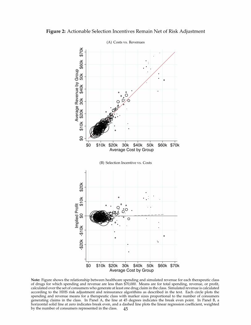
Figure 2: Actionable Selection Incentives Remain Net of Risk Adjustment

(A) Costs vs. Revenues

$0$1

0k$2

0k30

k$4

0k50

k$6

0k$7

0kAv

erag

e R

even

ue b

y G

roup

$0 $10k $20k 30k $40k 50k $60k $70kAverage Cost by Group

(B) Selection Incentive vs. Costs

-$

20k

-$10

k $0

$10k

$20k

Im

plie

d Pr

ofit

$0 $10k $20k 30k $40k 50k $60k $70kAverage Cost by Group

Note: Figure shows the relationship between healthcare spending and simulated revenue for each therapeutic classof drugs for which spending and revenue are less than $70,000. Means are for total spending, revenue, or profit,calculated over the set of consumers who generate at least one drug claim in the class. Simulated revenue is calculatedaccording to the HHS risk adjustment and reinsurance algorithms as described in the text. Each circle plots thespending and revenue means for a therapeutic class with marker sizes proportional to the number of consumersgenerating claims in the class. In Panel A, the line at 45 degrees indicates the break even point. In Panel B, ahorizontal solid line at zero indicates break even, and a dashed line plots the linear regression coefficient, weightedby the number of consumers represented in the class. 45

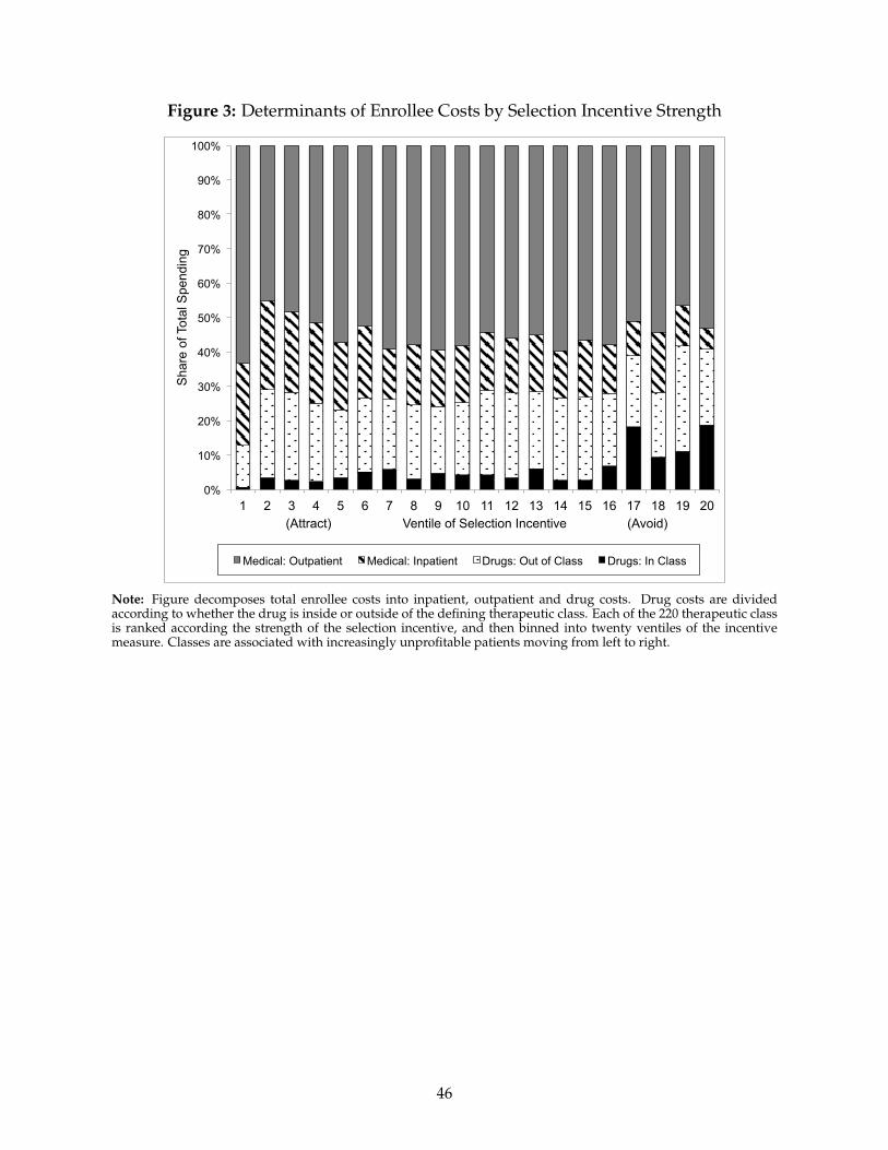
Figure 3: Determinants of Enrollee Costs by Selection Incentive Strength

0%

10%

20%

30%

40%

50%

60%

70%

80%

90%

100%

1 2 3 4 5 6 7 8 9 10 11 12 13 14 15 16 17 18 19 20

Sha

re o

f Tot

al S

pend

ing

(Attract) Ventile of Selection Incentive (Avoid)

Medical: Outpatient Medical: Inpatient Drugs: Out of Class Drugs: In Class

Note: Figure decomposes total enrollee costs into inpatient, outpatient and drug costs. Drug costs are dividedaccording to whether the drug is inside or outside of the defining therapeutic class. Each of the 220 therapeutic classis ranked according the strength of the selection incentive, and then binned into twenty ventiles of the incentivemeasure. Classes are associated with increasingly unprofitable patients moving from left to right.

46

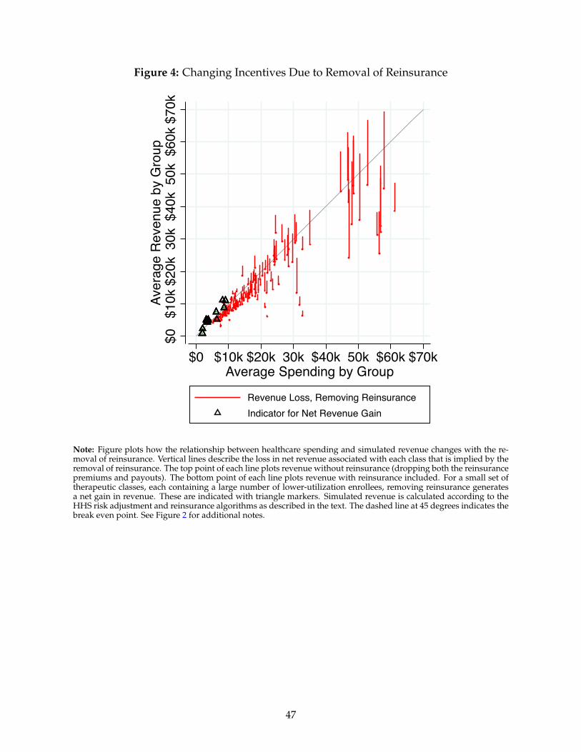
Figure 4: Changing Incentives Due to Removal of Reinsurance

$0$1

0k$2

0k30

k$4

0k50

k$6

0k$7

0kAv

erag

e R

even

ue b

y G

roup

$0 $10k $20k 30k $40k 50k $60k $70kAverage Spending by Group

Revenue Loss, Removing ReinsuranceIndicator for Net Revenue Gain

Note: Figure plots how the relationship between healthcare spending and simulated revenue changes with the re-moval of reinsurance. Vertical lines describe the loss in net revenue associated with each class that is implied by theremoval of reinsurance. The top point of each line plots revenue without reinsurance (dropping both the reinsurancepremiums and payouts). The bottom point of each line plots revenue with reinsurance included. For a small set oftherapeutic classes, each containing a large number of lower-utilization enrollees, removing reinsurance generatesa net gain in revenue. These are indicated with triangle markers. Simulated revenue is calculated according to theHHS risk adjustment and reinsurance algorithms as described in the text. The dashed line at 45 degrees indicates thebreak even point. See Figure 2 for additional notes.

47

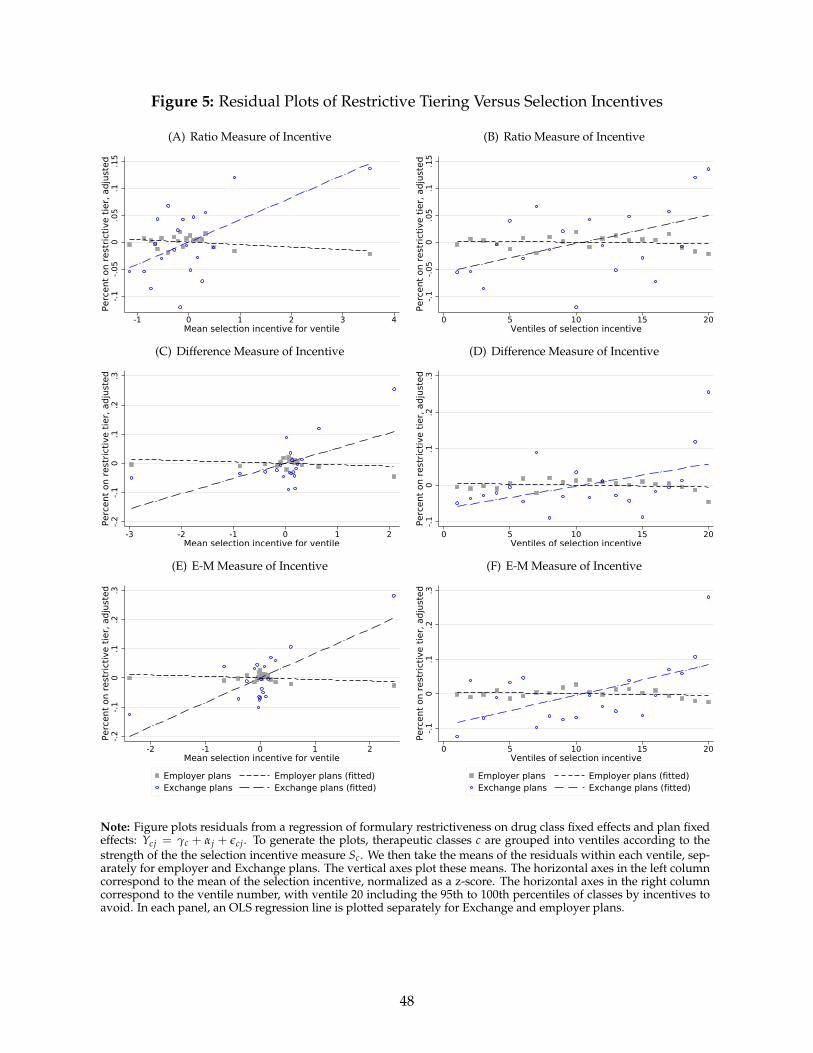
Figure 5: Residual Plots of Restrictive Tiering Versus Selection Incentives

(A) Ratio Measure of Incentive

-.1-.0

50

.05

.1.1

5Pe

rcen

t on

rest

rictiv

e tie

r, ad

just

ed

-1 0 1 2 3 4Mean selection incentive for ventile

Employer plans Employer plans (fitted)Exchange plans Exchange plans (fitted)

(B) Ratio Measure of Incentive

-.1-.0

50

.05

.1.1

5Pe

rcen

t on

rest

rictiv

e tie

r, ad

just

ed

0 5 10 15 20Ventiles of selection incentive

Employer plans Employer plans (fitted)Exchange plans Exchange plans (fitted)(C) Difference Measure of Incentive

-.2-.1

0.1

.2.3

Perc

ent o

n re

stric

tive

tier,

adju

sted

-3 -2 -1 0 1 2Mean selection incentive for ventile

Employer plans Employer plans (fitted)Exchange plans Exchange plans (fitted)

(D) Difference Measure of Incentive

-.10

.1.2

.3Pe

rcen

t on

rest

rictiv

e tie

r, ad

just

ed

0 5 10 15 20Ventiles of selection incentive

Employer plans Employer plans (fitted)Exchange plans Exchange plans (fitted)(E) E-M Measure of Incentive

-.2-.1

0.1

.2.3

Perc

ent o

n re

stric

tive

tier,

adju

sted

-2 -1 0 1 2Mean selection incentive for ventile

Employer plans Employer plans (fitted)Exchange plans Exchange plans (fitted)

(F) E-M Measure of Incentive

-.10

.1.2

.3Pe

rcen

t on

rest

rictiv

e tie

r, ad

just

ed

0 5 10 15 20Ventiles of selection incentive

Employer plans Employer plans (fitted)Exchange plans Exchange plans (fitted)

Note: Figure plots residuals from a regression of formulary restrictiveness on drug class fixed effects and plan fixedeffects: Ycj = γc + αj + εcj. To generate the plots, therapeutic classes c are grouped into ventiles according to thestrength of the the selection incentive measure Sc. We then take the means of the residuals within each ventile, sep-arately for employer and Exchange plans. The vertical axes plot these means. The horizontal axes in the left columncorrespond to the mean of the selection incentive, normalized as a z-score. The horizontal axes in the right columncorrespond to the ventile number, with ventile 20 including the 95th to 100th percentiles of classes by incentives toavoid. In each panel, an OLS regression line is plotted separately for Exchange and employer plans.

48

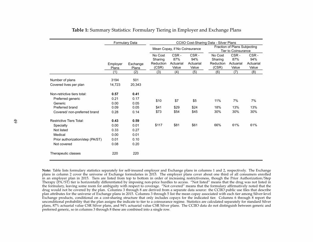
Table 1: Summary Statistics: Formulary Tiering in Employer and Exchange Plans

No Cost Sharing

Reduction (CSR)

CSR - 87%

Actuarial Value

CSR - 94%

Actuarial Value

No Cost Sharing

Reduction (CSR)

CSR - 87%

Actuarial Value

CSR - 94%

Actuarial Value

(1) (2) (3) (4) (5) (6) (7) (8)

Number of plans 3194 501Covered lives per plan 14,723 20,343

Non-retrictive tiers total: 0.57 0.41Preferred generic 0.21 0.17Generic 0.00 0.05Preferred brand 0.09 0.05 $41 $29 $24 18% 13% 13%Covered/ non-preferred brand 0.28 0.14 $73 $54 $45 30% 30% 30%

Restrictive Tiers Total: 0.43 0.59Specialty 0.00 0.01 $117 $81 $61 66% 61% 61%Not listed 0.33 0.27Medical 0.00 0.01Prior authorization/step (PA/ST) 0.01 0.10Not covered 0.08 0.20

Therapeutic classes 220 220

Formulary Data

$5 7%$10 $7 11% 7%

Mean Copay, if No Coinsurance Fraction of Plans Subjecting Tier to Coinsurance

CCIIO Cost-Sharing Data - Silver Plans

Exchange Plans

Employer Plans

Note: Table lists formulary statistics separately for self-insured employer and Exchange plans in columns 1 and 2, respectively. The Exchangeplans in column 2 cover the universe of Exchange formularies in 2015. The employer plans cover about one third of all consumers enrolledin an employer plan in 2015. Tiers are listed from top to bottom in order of increasing restrictiveness, though the Prior Authorization/StepTherapy (PA/ST) tier is horizontally differentiated by imposing non-price hurdles to access. “Not listed” means that the drug was not listed inthe formulary, leaving some room for ambiguity with respect to coverage. “Not covered” means that the formulary affirmatively noted that thedrug would not be covered by the plan. Columns 3 through 8 are derived from a separate data source: the CCIIO public use files that describeplan attributes for the universe of Exchange plans in 2015. Columns 3 through 5 list the mean copay associated with each tier among Silver-levelExchange products, conditional on a cost-sharing structure that only includes copays for the indicated tier. Columns 6 through 8 report theunconditional probability that the plan assigns the indicate to tier to a coinsurance regime. Statistics are calculated separately for standard Silverplans, 87% actuarial value CSR Silver plans, and 94% actuarial value CSR Silver plans. The CCIIO data do not distinguish between generic andpreferred generic, so in columns 3 through 8 these are combined into a single row.

49

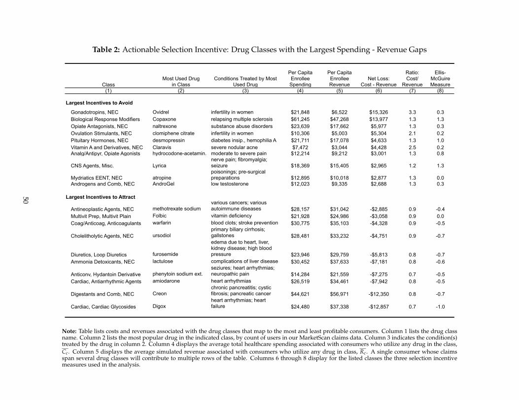
Table 2: Actionable Selection Incentive: Drug Classes with the Largest Spending - Revenue Gaps

ClassMost Used Drug

in ClassConditions Treated by Most

Used Drug

Per Capita Enrollee Spending

Per Capita Enrollee Revenue

Net Loss: Cost - Revenue

Ratio: Cost/

Revenue

Ellis-McGuire Measure

(1) (2) (3) (4) (5) (6) (7) (8)

Largest Incentives to Avoid

Gonadotropins, NEC Ovidrel infertility in women $21,848 $6,522 $15,326 3.3 0.3Biological Response Modifiers Copaxone relapsing multiple sclerosis $61,245 $47,268 $13,977 1.3 1.3Opiate Antagonists, NEC naltrexone substance abuse disorders $23,639 $17,662 $5,977 1.3 0.3Ovulation Stimulants, NEC clomiphene citrate infertility in women $10,306 $5,003 $5,304 2.1 0.2Pituitary Hormones, NEC desmopressin diabetes insip., hemophilia A $21,711 $17,078 $4,633 1.3 1.0Vitamin A and Derivatives, NEC Claravis severe nodular acne $7,472 $3,044 $4,428 2.5 0.2Analg/Antipyr, Opiate Agonists hydrocodone-acetamin. moderate to severe pain $12,214 $9,212 $3,001 1.3 0.8

CNS Agents, Misc. Lyricanerve pain; fibromyalgia; seizure $18,369 $15,405 $2,965 1.2 1.3

Mydriatics EENT, NEC atropinepoisonings; pre-surgical preparations $12,895 $10,018 $2,877 1.3 0.0

Androgens and Comb, NEC AndroGel low testosterone $12,023 $9,335 $2,688 1.3 0.3

Largest Incentives to Attract

Antineoplastic Agents, NEC methotrexate sodiumvarious cancers; various autoimmune diseases $28,157 $31,042 -$2,885 0.9 -0.4

Multivit Prep, Multivit Plain Folbic vitamin deficiency $21,928 $24,986 -$3,058 0.9 0.0Coag/Anticoag, Anticoagulants warfarin blood clots; stroke prevention $30,775 $35,103 -$4,328 0.9 -0.5

Cholelitholytic Agents, NEC ursodiolprimary biliary cirrhosis; gallstones $28,481 $33,232 -$4,751 0.9 -0.7

Diuretics, Loop Diuretics furosemide

edema due to heart, liver, kidney disease; high blood pressure $23,946 $29,759 -$5,813 0.8 -0.7

Ammonia Detoxicants, NEC lactulose complications of liver disease $30,452 $37,633 -$7,181 0.8 -0.6

Anticonv, Hydantoin Derivative phenytoin sodium ext.seziures; heart arrhythmias; neuropathic pain $14,284 $21,559 -$7,275 0.7 -0.5

Cardiac, Antiarrhythmic Agents amiodarone heart arrhythmias $26,519 $34,461 -$7,942 0.8 -0.5

Digestants and Comb, NEC Creonchronic pancreatitis; cystic fibrosis; pancreatic cancer $44,621 $56,971 -$12,350 0.8 -0.7

Cardiac, Cardiac Glycosides Digoxheart arrhythmias; heart failure $24,480 $37,338 -$12,857 0.7 -1.0

Note: Table lists costs and revenues associated with the drug classes that map to the most and least profitable consumers. Column 1 lists the drug classname. Column 2 lists the most popular drug in the indicated class, by count of users in our MarketScan claims data. Column 3 indicates the condition(s)treated by the drug in column 2. Column 4 displays the average total healthcare spending associated with consumers who utilize any drug in the class,Cc. Column 5 displays the average simulated revenue associated with consumers who utilize any drug in class, Rc. A single consumer whose claimsspan several drug classes will contribute to multiple rows of the table. Columns 6 through 8 display for the listed classes the three selection incentivemeasures used in the analysis.

50

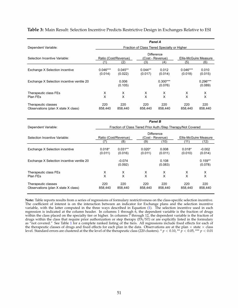
Table 3: Main Result: Selection Incentive Predicts Restrictive Design in Exchanges Relative to ESI

Dependent Variable:

Selection Incentive Variable:(1) (2) (3) (4) (5) (6)

Exchange X Selection incentive 0.046*** 0.045** 0.044** 0.012 0.046*** 0.010(0.014) (0.022) (0.017) (0.014) (0.018) (0.015)

Exchange X Selection incentive ventile 20 0.006 0.300*** 0.296***(0.105) (0.076) (0.089)

Therapeutic class FEs X X X X X XPlan FEs X X X X X X

Therapeutic classes 220 220 220 220 220 220Observations (plan X state X class) 858,440 858,440 858,440 858,440 858,440 858,440

Dependent Variable:

Selection Incentive Variable:(7) (8) (9) (10) (11) (12)

Exchange X Selection incentive 0.018* 0.031** 0.020* 0.008 0.018* -0.002(0.011) (0.016) (0.011) (0.011) (0.010) (0.014)

Exchange X Selection incentive ventile 20 -0.074 0.108 0.159**(0.092) (0.083) (0.078)

Therapeutic class FEs X X X X X XPlan FEs X X X X X X

Therapeutic classes 220 220 220 220 220 220Observations (plan X state X class) 858,440 858,440 858,440 858,440 858,440 858,440

Fraction of Class Tiered Specialty or Higher

Panel A

Panel B

Difference (Cost - Revenue) Ellis-McGuire Measure

Difference (Cost - Revenue) Ellis-McGuire Measure

Fraction of Class Tiered Prior Auth./Step Therapy/Not Covered

Ratio (Cost/Revenue)

Ratio (Cost/Revenue)

Note: Table reports results from a series of regressions of formulary restrictiveness on the class-specific selection incentive.The coefficient of interest is on the interaction between an indicator for Exchange plans and the selection incentivevariable, with the latter computed in the three ways described in Equation (1). The selection incentive used in eachregression is indicated at the column header. In columns 1 through 6, the dependent variable is the fraction of drugswithin the class placed on the specialty tier or higher. In columns 7 through 12, the dependent variable is the fraction ofdrugs within the class that require prior authorization or step therapy (PA/ST) or are explicitly listed in the formularyas “not covered.” See Table 1 for a complete ranked listing of the tiers. All regressions include fixed effects for each ofthe therapeutic classes of drugs and fixed effects for each plan in the data. Observations are at the plan × state × classlevel. Standard errors are clustered at the the level of the therapeutic class (220 clusters). * p < 0.10, ** p < 0.05, *** p < 0.01

51

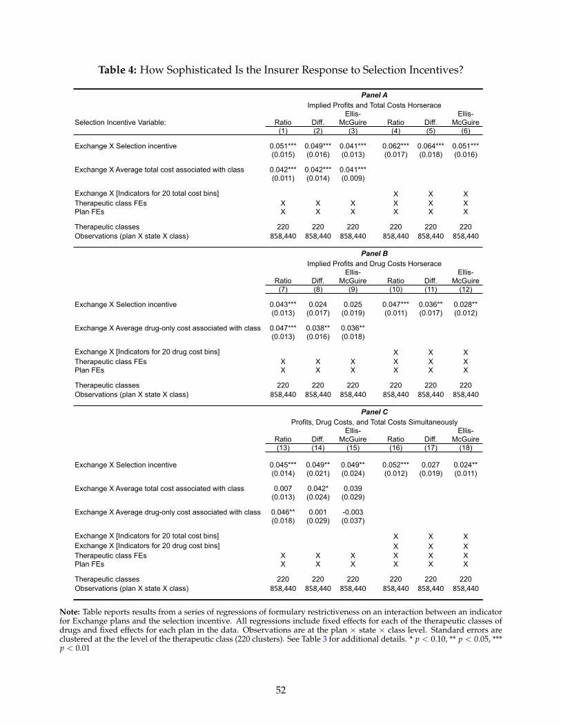
Table 4: How Sophisticated Is the Insurer Response to Selection Incentives?

Selection Incentive Variable: Ratio Diff.Ellis-

McGuire Ratio Diff.Ellis-

McGuire(1) (2) (3) (4) (5) (6)

Exchange X Selection incentive 0.051*** 0.049*** 0.041*** 0.062*** 0.064*** 0.051***(0.015) (0.016) (0.013) (0.017) (0.018) (0.016)

Exchange X Average total cost associated with class 0.042*** 0.042*** 0.041***(0.011) (0.014) (0.009)

Exchange X [Indicators for 20 total cost bins] X X XTherapeutic class FEs X X X X X XPlan FEs X X X X X X

Therapeutic classes 220 220 220 220 220 220Observations (plan X state X class) 858,440 858,440 858,440 858,440 858,440 858,440

Ratio Diff.Ellis-

McGuire Ratio Diff.Ellis-

McGuire(7) (8) (9) (10) (11) (12)

Exchange X Selection incentive 0.043*** 0.024 0.025 0.047*** 0.036** 0.028**(0.013) (0.017) (0.019) (0.011) (0.017) (0.012)

Exchange X Average drug-only cost associated with class 0.047*** 0.038** 0.036**(0.013) (0.016) (0.018)

Exchange X [Indicators for 20 drug cost bins] X X XTherapeutic class FEs X X X X X XPlan FEs X X X X X X

Therapeutic classes 220 220 220 220 220 220Observations (plan X state X class) 858,440 858,440 858,440 858,440 858,440 858,440

Ratio Diff.Ellis-

McGuire Ratio Diff.Ellis-

McGuire(13) (14) (15) (16) (17) (18)

Exchange X Selection incentive 0.045*** 0.049** 0.049** 0.052*** 0.027 0.024**(0.014) (0.021) (0.024) (0.012) (0.019) (0.011)

Exchange X Average total cost associated with class 0.007 0.042* 0.039(0.013) (0.024) (0.029)

Exchange X Average drug-only cost associated with class 0.046** 0.001 -0.003(0.018) (0.029) (0.037)

Exchange X [Indicators for 20 total cost bins] X X XExchange X [Indicators for 20 drug cost bins] X X XTherapeutic class FEs X X X X X XPlan FEs X X X X X X

Therapeutic classes 220 220 220 220 220 220Observations (plan X state X class) 858,440 858,440 858,440 858,440 858,440 858,440

Profits, Drug Costs, and Total Costs Simultaneously

Panel A

Implied Profits and Drug Costs Horserace

Implied Profits and Total Costs Horserace

Panel B

Panel C

Note: Table reports results from a series of regressions of formulary restrictiveness on an interaction between an indicatorfor Exchange plans and the selection incentive. All regressions include fixed effects for each of the therapeutic classes ofdrugs and fixed effects for each plan in the data. Observations are at the plan × state × class level. Standard errors areclustered at the the level of the therapeutic class (220 clusters). See Table 3 for additional details. * p < 0.10, ** p < 0.05, ***p < 0.01

52

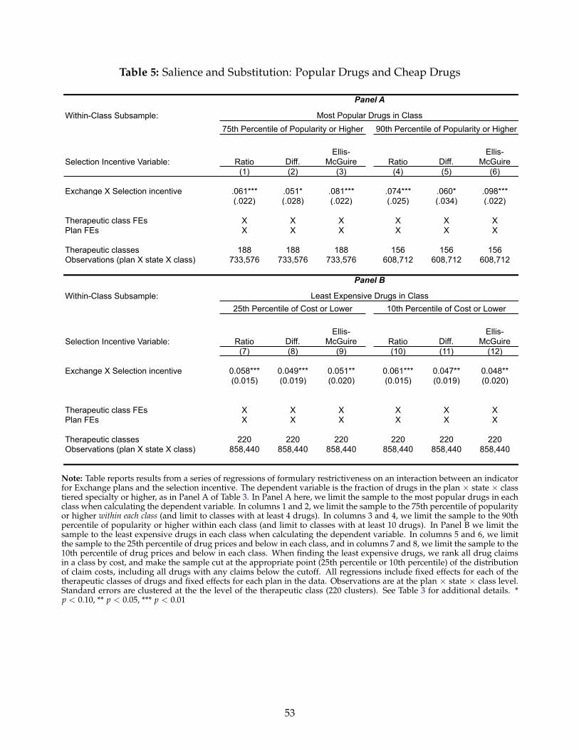
Table 5: Salience and Substitution: Popular Drugs and Cheap Drugs

Within-Class Subsample:

Selection Incentive Variable: Ratio Diff.Ellis-

McGuire Ratio Diff.Ellis-

McGuire(1) (2) (3) (4) (5) (6)

Exchange X Selection incentive .061*** .051* .081*** .074*** .060* .098***(.022) (.028) (.022) (.025) (.034) (.022)

Therapeutic class FEs X X X X X XPlan FEs X X X X X X

Therapeutic classes 188 188 188 156 156 156Observations (plan X state X class) 733,576 733,576 733,576 608,712 608,712 608,712

Within-Class Subsample:

Selection Incentive Variable: Ratio Diff.Ellis-

McGuire Ratio Diff.Ellis-

McGuire(7) (8) (9) (10) (11) (12)

Exchange X Selection incentive 0.058*** 0.049*** 0.051** 0.061*** 0.047** 0.048**(0.015) (0.019) (0.020) (0.015) (0.019) (0.020)

Therapeutic class FEs X X X X X XPlan FEs X X X X X X

Therapeutic classes 220 220 220 220 220 220Observations (plan X state X class) 858,440 858,440 858,440 858,440 858,440 858,440

Panel B

Least Expensive Drugs in Class25th Percentile of Cost or Lower 10th Percentile of Cost or Lower

Panel A

Most Popular Drugs in Class75th Percentile of Popularity or Higher 90th Percentile of Popularity or Higher

Note: Table reports results from a series of regressions of formulary restrictiveness on an interaction between an indicatorfor Exchange plans and the selection incentive. The dependent variable is the fraction of drugs in the plan × state × classtiered specialty or higher, as in Panel A of Table 3. In Panel A here, we limit the sample to the most popular drugs in eachclass when calculating the dependent variable. In columns 1 and 2, we limit the sample to the 75th percentile of popularityor higher within each class (and limit to classes with at least 4 drugs). In columns 3 and 4, we limit the sample to the 90thpercentile of popularity or higher within each class (and limit to classes with at least 10 drugs). In Panel B we limit thesample to the least expensive drugs in each class when calculating the dependent variable. In columns 5 and 6, we limitthe sample to the 25th percentile of drug prices and below in each class, and in columns 7 and 8, we limit the sample to the10th percentile of drug prices and below in each class. When finding the least expensive drugs, we rank all drug claimsin a class by cost, and make the sample cut at the appropriate point (25th percentile or 10th percentile) of the distributionof claim costs, including all drugs with any claims below the cutoff. All regressions include fixed effects for each of thetherapeutic classes of drugs and fixed effects for each plan in the data. Observations are at the plan × state × class level.Standard errors are clustered at the the level of the therapeutic class (220 clusters). See Table 3 for additional details. *p < 0.10, ** p < 0.05, *** p < 0.01

53

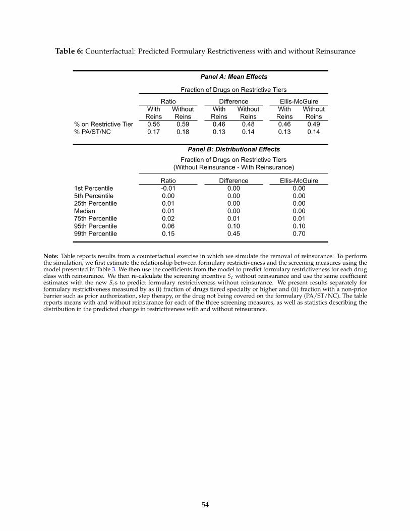
Table 6: Counterfactual: Predicted Formulary Restrictiveness with and without Reinsurance

With Reins

Without Reins

With Reins

Without Reins

With Reins

Without Reins

% on Restrictive Tier 0.56 0.59 0.46 0.48 0.46 0.49% PA/ST/NC 0.17 0.18 0.13 0.14 0.13 0.14

1st Percentile5th Percentile25th PercentileMedian75th Percentile95th Percentile99th Percentile

Fraction of Drugs on Restrictive Tiers

Panel A: Mean Effects

Fraction of Drugs on Restrictive Tiers (Without Reinsurance - With Reinsurance)

Panel B: Distributional Effects

0.01 0.00

-0.01 0.000.00 0.00

0.000.01 0.00

Ratio Difference Ellis-McGuire

0.010.100.700.15 0.45

0.02 0.010.06 0.10

0.00

Ratio Difference Ellis-McGuire0.000.00

Note: Table reports results from a counterfactual exercise in which we simulate the removal of reinsurance. To performthe simulation, we first estimate the relationship between formulary restrictiveness and the screening measures using themodel presented in Table 3. We then use the coefficients from the model to predict formulary restrictiveness for each drugclass with reinsurance. We then re-calculate the screening incentive Sc without reinsurance and use the same coefficientestimates with the new Scs to predict formulary restrictiveness without reinsurance. We present results separately forformulary restrictiveness measured by as (i) fraction of drugs tiered specialty or higher and (ii) fraction with a non-pricebarrier such as prior authorization, step therapy, or the drug not being covered on the formulary (PA/ST/NC). The tablereports means with and without reinsurance for each of the three screening measures, as well as statistics describing thedistribution in the predicted change in restrictiveness with and without reinsurance.

54

Online Appendix A MODEL

Online Appendix for:Screening in Contract Design:

Evidence from the ACA Health Insurance Exchanges

by Michael Geruso, Timothy Layton, and Daniel Prinz

A Model

In this section, we present a formal model of the contract design problem of a profit-maximizinginsurer in the setting where the insurer offers only one contract, must charge the same premiumto all enrollees (community rating), and cannot prohibit any consumer who desires to purchase thecontract from enrolling (guaranteed issue). We show that in this setting, the equilibrium contractdiffers from the socially efficient contract and that the size of the distortion is related to the correlationbetween the use of the distorted health care service and a consumer’s profitability. We note that thismodel is a more general version of the simple model described in Section 2.

We start by following much of the prior literature in assuming that insurers offer a single contractthat consists of a price p and a coinsurance rate 1− x, so that x ∈ [0, 1] is the portion of spendingpaid by the insurer. In our context, this can be thought of as an insurance contract providing partialcoverage for spending on one drug.77 Each individual faces a distribution of potential drug spend-ing with mean µ and variance σ2. We most closely follow Veiga and Weyl (2016) in specifying anindividual’s expected cost to the insurer as the product of two components: a fixed component µ,and a component k(x) that varies with coverage and incorporates both the direct effect of coverageon insurer costs (a smaller x implies that the insurer pays a smaller portion of the cost of the drug)and the indirect moral hazard effect (a smaller x induces less consumption of the drug). Formally,cj = µk(xj) is the expected cost to insurer j. We assume that the components are independent so thatk(x) does not vary with µ.

Define v as the product of the coefficient of absolute risk aversion and the variance of the spend-ing distribution, σ2, so that v is related to the expected utility cost of anticipated risk. Veiga and Weyl(2016) show that under the assumption of CARA utility, willingness-to-pay for coverage x is givenby

u = µh(x) + vψ(x), (5)

where µh(x) is the benefit the individual gets from insurer spending equal to µk(x), and vψ(x) is thebenefit the individual gets from the level of risk protection offered by the contract.

In this environment, with a distribution of consumer types defined by f (µ, v), social welfare canbe described with the following expression:

W =∫

µ

∫v

f (µ, v)[µh(x) + vψ(x)− µk(x)]dv dµ. (6)

The additional term between Equations (5) and (6) is µk(x), which captures the cost of coverage,including that due to moral hazard. It is straightforward to show that in order to maximize socialwelfare, the social planner would set coverage generosity x∗ to solve the following equality:

ψ′(x∗) = φ(k′(x∗)− h′(x∗)), (7)

77Empirically, we consider contracts with many such cost sharing parameters for many drugs, but the one parameterframework is common in the literature and sufficient to highlight the core intuitions here.

1

Online Appendix A MODEL

where φ = E[µ]E[v] . This is the classic trade-off between the benefits of risk protection, ψ′(x∗), and the

social cost of moral hazard, k′(x∗)− h′(x∗), as first pointed out by Zeckhauser (1970) and Feldstein(1973).

We next consider insurer j’s choice of x in a competitive health insurance market. We specifyinsurer j’s profit function as

π j =∫

µ

∫v

f (µ, v)D(xj; µ, v)[r(xj, µ, v)− µk(xj)]dv dµ, (8)

where D(xj; µ, v) is demand—the probability of enrollment in a plan with coinsurance rate 1− xj foran individual of type (µ, v). The term r(xj, µ, v) is the payment the plan gets for an individual oftype (µ, v), including risk adjustment, reinsurance, or any other regulatory transfer or payment. Asabove, µk(xj) denotes the cost of providing insurance.

The insurer sets the portion of spending it covers, xj, to maximize profits. To understand theinsurer’s problem, we differentiate π j with respect to xj holding the premium fixed:

∂π j

∂xj =∫

µ

∫v

f (µ, v)[

∂D(xj; µ, v)∂xj

(r(xj, µ, v)− µk(xj)

)− µk′(xj)D(xj; µ, v)

]dvdµ. (9)

The derivative consists of two components inside the brackets. The first component captures changesin demand (i.e. enrollment) due to a change in the portion of spending covered by the plan, xj. Thesecond component captures the change in plan spending among the existing enrollee population.78

The demand effect (the first term in brackets in equation 9) can be further decomposed to revealtwo distinct demand-related consequences of a change in xj. If we define r = E[r(xj, µ, v)] andc = E[µk(xj)] as the average net revenue and the average cost (for a given xj) across the entirepopulation, then:

∂D(xj; µ, v)∂xj (r(xj, µ, v)− µk(xj)) =

∂D(xj; µ, v)∂xj [r− c]︸ ︷︷ ︸

More enrollees

+∂D(xj; µ, v)

∂xj [(r(xj, µ, v)− µk(xj))− (r− c)]︸ ︷︷ ︸Different enrollees

.

(10)The “more enrollees” term above represents the change in insurer profits due to a change in thenumber of individuals of average profitability enrolled in the plan. This arises because consumers’willingness-to-pay for the plan, as described by Equation (5), varies with the plan generosity. Impor-tantly, this component is related to the social planner’s problem because valuation in excess of costwill increase as xj converges to the social optimum. The “different enrollees” component reveals thatthe insurer has an additional consideration in setting x, beyond trading off risk protection and moralhazard: The plan will attract marginal enrollees who may be differentially profitable to the insurerdepending on their specific payments and costs.

Note that if the “different enrollees” term is zero, then the insurer solving the first order conditionin Equation (10) under a symmetric competitive equilibrium will decrease the coinsurance rate (1−xj) until the additional profits from enrolling more individuals equals the additional costs due toproviding better coverage. This parallels the social planner’s problem of trading off the benefitsof risk protection with the cost of moral hazard.79 In fact, Einav, Finkelstein and Polyakova (2016)

78The change in spending among existing enrollees is due to both the direct effect of the increase in the portion ofspending covered by the plan and the indirect effect of the increase in the individual’s total spending caused by moralhazard.

79To see this, let the demand function be described as D(xj; µ, v) = G(uj = µh(xj) + vψ(xj)). This implies that∂D(xj ;µ,v)

∂xj = G′[µh′(xj) + vψ′(xj)]. It is now straightforward to see that the same expression for the social benefit that

2

Online Appendix B SIMULATED PAYMENTS

show via simulation that the social planner’s problem and that of the profit-maximizing firm coincidewhen the “different enrollees” term is zero, with both trading off the social costs and benefits of moregenerous insurance.

The possibility of screening types by setting the coinsurance rate thus represents a margin thatdrives a wedge between the level at which a profit-maximizing insurer sets the coinsurance rate andthe socially efficient level. Though we merely sketch the intuition here, this result is shown rigorouslyby Glazer and McGuire (2000), Frank, Glazer and McGuire (2000), and Veiga and Weyl (2016), whoalso show that the size of the wedge is proportional to the covariance among marginal consumersbetween willingness-to-pay for coverage and the consumer’s cost to the insurer. Ellis and McGuire(2007) devise a practical empirical metric that reflects this covariance, which we follow when weempirically operationalize the insurer’s selection incentive.

B Simulated payments

This section provides more detail on the simulated payments used to compute selection incentivesand the HHS-HCC risk adjustment model.

We define costs as the sum of all health care spending (inpatient, outpatient, and prescriptiondrug) for person i in a given year. We observe this in the Marketscan data. Revenues are not observedin the data and must be simulated. We simulate revenues according to Exchange plan paymentformulas specified by the Department of Health and Human Services (HHS). Exchange plan revenuesfor plan j consist of three components: premiums, pj

i , risk adjustment transfers, RRAi , and reinsurance

payments RRei .

For risk adjustment transfers, we start by specifying a risk score, ri, for each individual using therisk adjustment formula used in the Exchanges (Kautter et al., 2014). This formula assigns risk scoresaccording to diagnoses in claims data. We use an individual’s diagnoses from 2012 to assign his/herrisk score. We then specify risk adjustment transfers according to the Exchange risk adjustmenttransfer formula:80

RRAi =

(ri

r− 1)

p,

where r = 1n ∑n

i=1 ri and p = 1n ∑n

i=1 pji are the average risk score and average premium across all

individuals in the market, respectively. Similarly, we define reinsurance payments as

RRei = .8×

(Ci − 60, 000

)for claim costs above $60,000.81 We assume that reinsurance is funded by an actuarially fair

per capita reinsurance premium, re.82 In words, the reinsurance payment is 80% of the individual

enters the social planner’s problem (µh′(xj) + vψ′(xj)) also enters the insurer’s profit maximization problem. It is alsostraightforward to see in Equation (10) above that the same expression for the social cost that enters the social planner’sproblem (µk′(xj)) also enters the insurer’s profit maximization problem. While the expressions differ in other ways, thereare clear similarities that lead the level of coverage chosen by a profit maximizing insurer to mimic the level chosen by thesocial planner.

80Note that risk adjustment transfers occur at the plan level, but in fact they are a sum of individual-level transfers. Herewe specify the component of the plan’s transfer attached to individual i.

81A policy with a cutoff of $60,000 and a coinsurance rate of 0.8 was the originally announced reinsurance policy forthe Exchanges. This was later adjusted ex post to a cutoff of $45,000 and a coinsurance rate of 0.5. We use the originallyannounced policy, as insurers likely designed their formularies according to the announced policy rather than the oneimplemented ex post. In practice, there is little difference between the two policies for insurer incentives.

82In practice, the Exchange reinsurance program is also funded by a similar premium, but it is assessed across almost all

3

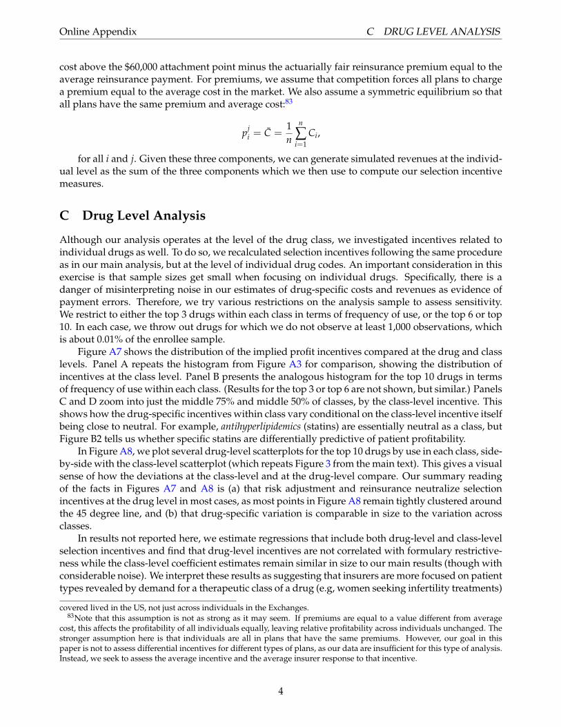
Online Appendix C DRUG LEVEL ANALYSIS

cost above the $60,000 attachment point minus the actuarially fair reinsurance premium equal to theaverage reinsurance payment. For premiums, we assume that competition forces all plans to chargea premium equal to the average cost in the market. We also assume a symmetric equilibrium so thatall plans have the same premium and average cost:83

pji = C =

1n

n

∑i=1

Ci,

for all i and j. Given these three components, we can generate simulated revenues at the individ-ual level as the sum of the three components which we then use to compute our selection incentivemeasures.

C Drug Level Analysis

Although our analysis operates at the level of the drug class, we investigated incentives related toindividual drugs as well. To do so, we recalculated selection incentives following the same procedureas in our main analysis, but at the level of individual drug codes. An important consideration in thisexercise is that sample sizes get small when focusing on individual drugs. Specifically, there is adanger of misinterpreting noise in our estimates of drug-specific costs and revenues as evidence ofpayment errors. Therefore, we try various restrictions on the analysis sample to assess sensitivity.We restrict to either the top 3 drugs within each class in terms of frequency of use, or the top 6 or top10. In each case, we throw out drugs for which we do not observe at least 1,000 observations, whichis about 0.01% of the enrollee sample.

Figure A7 shows the distribution of the implied profit incentives compared at the drug and classlevels. Panel A repeats the histogram from Figure A3 for comparison, showing the distribution ofincentives at the class level. Panel B presents the analogous histogram for the top 10 drugs in termsof frequency of use within each class. (Results for the top 3 or top 6 are not shown, but similar.) PanelsC and D zoom into just the middle 75% and middle 50% of classes, by the class-level incentive. Thisshows how the drug-specific incentives within class vary conditional on the class-level incentive itselfbeing close to neutral. For example, antihyperlipidemics (statins) are essentially neutral as a class, butFigure B2 tells us whether specific statins are differentially predictive of patient profitability.

In Figure A8, we plot several drug-level scatterplots for the top 10 drugs by use in each class, side-by-side with the class-level scatterplot (which repeats Figure 3 from the main text). This gives a visualsense of how the deviations at the class-level and at the drug-level compare. Our summary readingof the facts in Figures A7 and A8 is (a) that risk adjustment and reinsurance neutralize selectionincentives at the drug level in most cases, as most points in Figure A8 remain tightly clustered aroundthe 45 degree line, and (b) that drug-specific variation is comparable in size to the variation acrossclasses.

In results not reported here, we estimate regressions that include both drug-level and class-levelselection incentives and find that drug-level incentives are not correlated with formulary restrictive-ness while the class-level coefficient estimates remain similar in size to our main results (though withconsiderable noise). We interpret these results as suggesting that insurers are more focused on patienttypes revealed by demand for a therapeutic class of a drug (e.g, women seeking infertility treatments)

covered lived in the US, not just across individuals in the Exchanges.83Note that this assumption is not as strong as it may seem. If premiums are equal to a value different from average

cost, this affects the profitability of all individuals equally, leaving relative profitability across individuals unchanged. Thestronger assumption here is that individuals are all in plans that have the same premiums. However, our goal in thispaper is not to assess differential incentives for different types of plans, as our data are insufficient for this type of analysis.Instead, we seek to assess the average incentive and the average insurer response to that incentive.

4

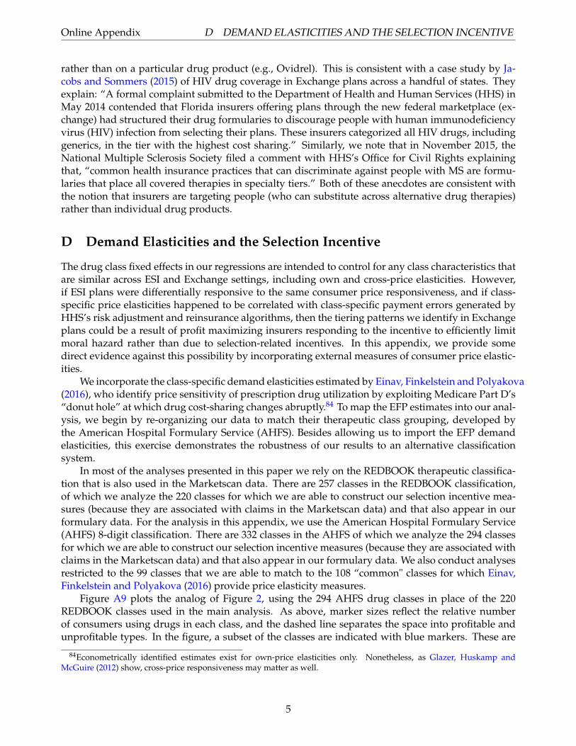
Online Appendix D DEMAND ELASTICITIES AND THE SELECTION INCENTIVE

rather than on a particular drug product (e.g., Ovidrel). This is consistent with a case study by Ja-cobs and Sommers (2015) of HIV drug coverage in Exchange plans across a handful of states. Theyexplain: “A formal complaint submitted to the Department of Health and Human Services (HHS) inMay 2014 contended that Florida insurers offering plans through the new federal marketplace (ex-change) had structured their drug formularies to discourage people with human immunodeficiencyvirus (HIV) infection from selecting their plans. These insurers categorized all HIV drugs, includinggenerics, in the tier with the highest cost sharing.” Similarly, we note that in November 2015, theNational Multiple Sclerosis Society filed a comment with HHS’s Office for Civil Rights explainingthat, “common health insurance practices that can discriminate against people with MS are formu-laries that place all covered therapies in specialty tiers.” Both of these anecdotes are consistent withthe notion that insurers are targeting people (who can substitute across alternative drug therapies)rather than individual drug products.

D Demand Elasticities and the Selection Incentive

The drug class fixed effects in our regressions are intended to control for any class characteristics thatare similar across ESI and Exchange settings, including own and cross-price elasticities. However,if ESI plans were differentially responsive to the same consumer price responsiveness, and if class-specific price elasticities happened to be correlated with class-specific payment errors generated byHHS’s risk adjustment and reinsurance algorithms, then the tiering patterns we identify in Exchangeplans could be a result of profit maximizing insurers responding to the incentive to efficiently limitmoral hazard rather than due to selection-related incentives. In this appendix, we provide somedirect evidence against this possibility by incorporating external measures of consumer price elastic-ities.

We incorporate the class-specific demand elasticities estimated by Einav, Finkelstein and Polyakova(2016), who identify price sensitivity of prescription drug utilization by exploiting Medicare Part D’s“donut hole” at which drug cost-sharing changes abruptly.84 To map the EFP estimates into our anal-ysis, we begin by re-organizing our data to match their therapeutic class grouping, developed bythe American Hospital Formulary Service (AHFS). Besides allowing us to import the EFP demandelasticities, this exercise demonstrates the robustness of our results to an alternative classificationsystem.

In most of the analyses presented in this paper we rely on the REDBOOK therapeutic classifica-tion that is also used in the Marketscan data. There are 257 classes in the REDBOOK classification,of which we analyze the 220 classes for which we are able to construct our selection incentive mea-sures (because they are associated with claims in the Marketscan data) and that also appear in ourformulary data. For the analysis in this appendix, we use the American Hospital Formulary Service(AHFS) 8-digit classification. There are 332 classes in the AHFS of which we analyze the 294 classesfor which we are able to construct our selection incentive measures (because they are associated withclaims in the Marketscan data) and that also appear in our formulary data. We also conduct analysesrestricted to the 99 classes that we are able to match to the 108 “common" classes for which Einav,Finkelstein and Polyakova (2016) provide price elasticity measures.

Figure A9 plots the analog of Figure 2, using the 294 AHFS drug classes in place of the 220REDBOOK classes used in the main analysis. As above, marker sizes reflect the relative numberof consumers using drugs in each class, and the dashed line separates the space into profitable andunprofitable types. In the figure, a subset of the classes are indicated with blue markers. These are

84Econometrically identified estimates exist for own-price elasticities only. Nonetheless, as Glazer, Huskamp andMcGuire (2012) show, cross-price responsiveness may matter as well.

5

Online Appendix D DEMAND ELASTICITIES AND THE SELECTION INCENTIVE

the 99 classes for which EFP generate demand elasticity estimates that we can match to our data.85

For the whole sample of classes and for this demand elasticity subset in blue, there are significantoutliers above the dashed line, mirroring Figure 2.

In Table A10, we replicate the main results using the AHFS classification. We generate our selec-tion incentive measures exactly as above. In column (1) we include the full schedule of AHFS drugclasses. In column (2) we restrict to only those classes for which we can directly control for a demandelasticity. In column (3) we add controls for the EFP estimate of class-specific elasticity interactedwith the indicator for an Exchange plan. (The elasticity main effects are naturally absorbed by theclass fixed effects.) We repeat this ordering of specifications for each of the three selection incentivemeasures and for both of the dependent variables from Table 3. The findings of Table A10 mirrorthose of Table 3 in that unprofitable classes are differentially assigned to restrictive tiers in Exchangeplans. Most importantly, the addition of demand elasticity controls have essentially no effect on thecoefficient estimates of interest. For completeness, Appendix Figure A10 plots the semi-parametricversions of the regressions.86

To better understand these results, we examine the correlation between the demand elasticityestimates and the selection incentive measures. Figure A6 graphs scatterplots of elasticity versusselection incentive by class. The three panels correspond to the three measures of Smc. There is nosignificant correlation between the selection incentive generated by the payment system error and thedemand elasticity. Taken together, Table A10 and Figures A6, A9, and A10 provide strong evidencethat Exchange plans are not merely differentially responding to socially efficient profit-maximizingconsiderations regarding class-specific consumer moral hazard in a way that ESI plans are failing todo.

85Einav, Finkelstein and Polyakova (2016) generate demand elasticities for 108 AHFS classes. We can match these classesand generate our selection incentive and tiering variables for 99 of these.

86The specifications using the Ellis-McGuire measures do not produce significant effects under the linear specificationshown. Like the main results, however, there are significant non-linear effects for the E-M measure, concentrated amongthe most unprofitable classes.

6

Online Appendix E ADDITIONAL FIGURES AND TABLES

E Additional Figures and Tables

7

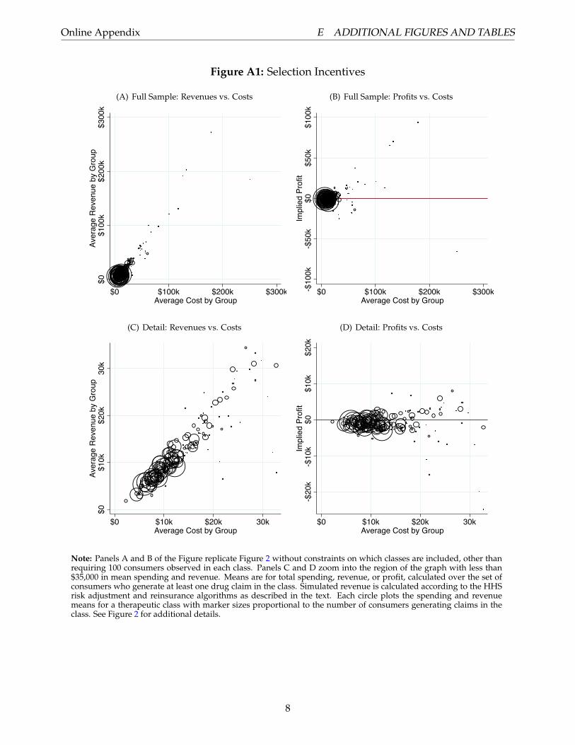
Online Appendix E ADDITIONAL FIGURES AND TABLES

Figure A1: Selection Incentives

(A) Full Sample: Revenues vs. Costs$0

$100

k$2

00k

$300

kAv

erag

e R

even

ue b

y G

roup

$0 $100k $200k $300kAverage Cost by Group

(B) Full Sample: Profits vs. Costs

-$10

0k-$

50k

$0$5

0k$1

00k

Impl

ied

Profi

t$0 $100k $200k $300k

Average Cost by Group

(C) Detail: Revenues vs. Costs

$0$1

0k$2

0k30

kAv

erag

e R

even

ue b

y G

roup

$0 $10k $20k 30kAverage Cost by Group

(D) Detail: Profits vs. Costs

-$20

k-$

10k

$0$1

0k$2

0kIm

plie

d Pr

ofit

$0 $10k $20k 30kAverage Cost by Group

Note: Panels A and B of the Figure replicate Figure 2 without constraints on which classes are included, other thanrequiring 100 consumers observed in each class. Panels C and D zoom into the region of the graph with less than$35,000 in mean spending and revenue. Means are for total spending, revenue, or profit, calculated over the set ofconsumers who generate at least one drug claim in the class. Simulated revenue is calculated according to the HHSrisk adjustment and reinsurance algorithms as described in the text. Each circle plots the spending and revenuemeans for a therapeutic class with marker sizes proportional to the number of consumers generating claims in theclass. See Figure 2 for additional details.

8

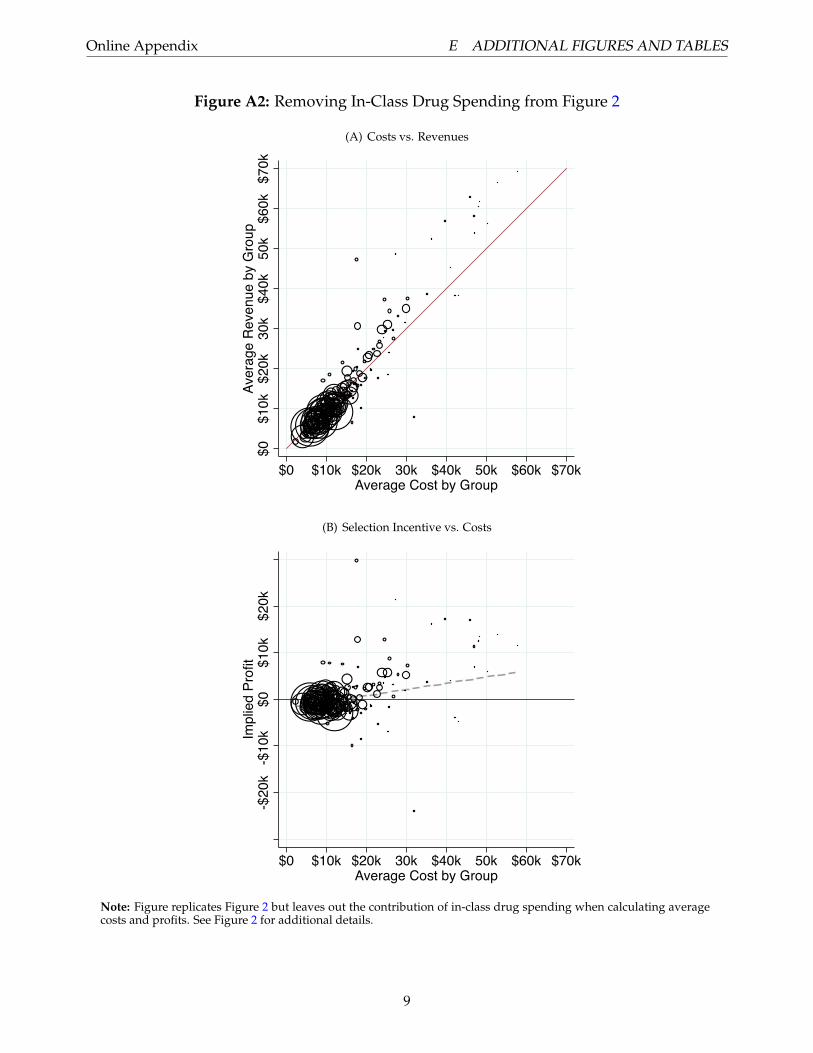
Online Appendix E ADDITIONAL FIGURES AND TABLES

Figure A2: Removing In-Class Drug Spending from Figure 2

(A) Costs vs. Revenues

$0$1

0k$2

0k30

k$4

0k50

k$6

0k$7

0kAv

erag

e R

even

ue b

y G

roup

$0 $10k $20k 30k $40k 50k $60k $70kAverage Cost by Group

(B) Selection Incentive vs. Costs

-$

20k

-$10

k $0

$10k

$20k

Im

plie

d Pr

ofit

$0 $10k $20k 30k $40k 50k $60k $70kAverage Cost by Group

Note: Figure replicates Figure 2 but leaves out the contribution of in-class drug spending when calculating averagecosts and profits. See Figure 2 for additional details.

9

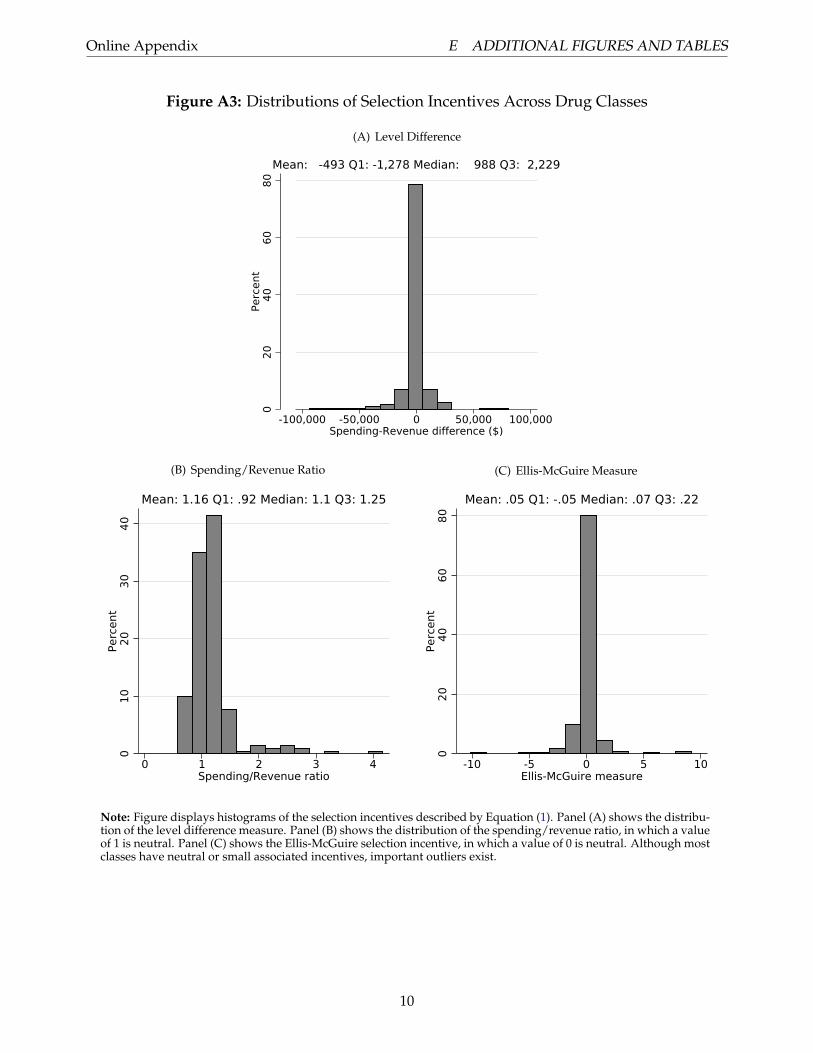
Online Appendix E ADDITIONAL FIGURES AND TABLES

Figure A3: Distributions of Selection Incentives Across Drug Classes

(A) Level Difference

020

4060

80Pe

rcen

t

-100,000 -50,000 0 50,000 100,000Spending-Revenue difference ($)

Mean: -493 Q1: -1,278 Median: 988 Q3: 2,229

(B) Spending/Revenue Ratio

010

2030

40Pe

rcen

t

0 1 2 3 4Spending/Revenue ratio

Mean: 1.16 Q1: .92 Median: 1.1 Q3: 1.25

(C) Ellis-McGuire Measure

020

4060

80Pe

rcen

t

-10 -5 0 5 10Ellis-McGuire measure

Mean: .05 Q1: -.05 Median: .07 Q3: .22

Note: Figure displays histograms of the selection incentives described by Equation (1). Panel (A) shows the distribu-tion of the level difference measure. Panel (B) shows the distribution of the spending/revenue ratio, in which a valueof 1 is neutral. Panel (C) shows the Ellis-McGuire selection incentive, in which a value of 0 is neutral. Although mostclasses have neutral or small associated incentives, important outliers exist.

10

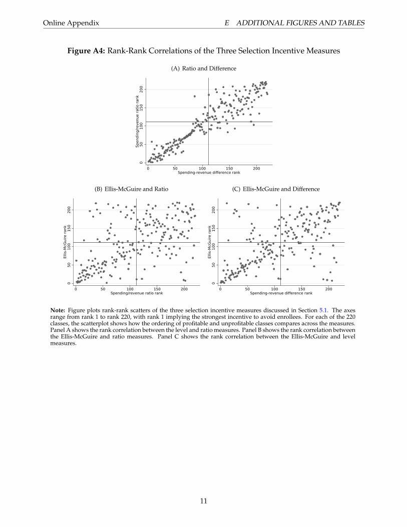
Online Appendix E ADDITIONAL FIGURES AND TABLES

Figure A4: Rank-Rank Correlations of the Three Selection Incentive Measures

(A) Ratio and Difference

050

100

150

200

Spen

ding

/rev

enue

ratio

rank

0 50 100 150 200Spending-revenue difference rank

(B) Ellis-McGuire and Ratio

050

100

150

200

Ellis

-McG

uire

rank

0 50 100 150 200Spending/revenue ratio rank

(C) Ellis-McGuire and Difference

050

100

150

200

Ellis

-McG

uire

rank

0 50 100 150 200Spending-revenue difference rank

Note: Figure plots rank-rank scatters of the three selection incentive measures discussed in Section 5.1. The axesrange from rank 1 to rank 220, with rank 1 implying the strongest incentive to avoid enrollees. For each of the 220classes, the scatterplot shows how the ordering of profitable and unprofitable classes compares across the measures.Panel A shows the rank correlation between the level and ratio measures. Panel B shows the rank correlation betweenthe Ellis-McGuire and ratio measures. Panel C shows the rank correlation between the Ellis-McGuire and levelmeasures.

11

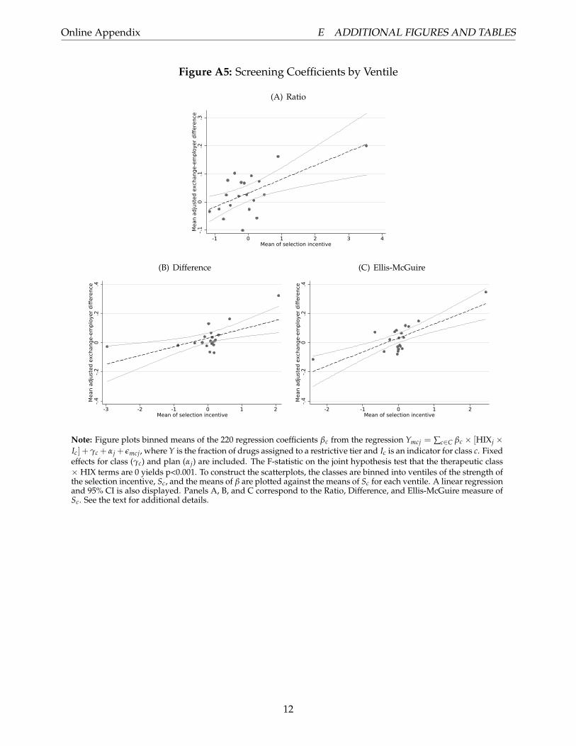
Online Appendix E ADDITIONAL FIGURES AND TABLES

Figure A5: Screening Coefficients by Ventile

(A) Ratio

-.10

.1.2

.3M

ean

adju

sted

exc

hang

e-em

ploy

er d

iffer

ence

-1 0 1 2 3 4Mean of selection incentive

(B) Difference

-.4-.2

0.2

.4M

ean

adju

sted

exc

hang

e-em

ploy

er d

iffer

ence

-3 -2 -1 0 1 2Mean of selection incentive

(C) Ellis-McGuire

-.4-.2

0.2

.4M

ean

adju

sted

exc

hang

e-em

ploy

er d

iffer

ence

-2 -1 0 1 2Mean of selection incentive

Note: Figure plots binned means of the 220 regression coefficients βc from the regression Ymcj = ∑c∈C βc × [HIXj ×Ic] +γc + αj + εmcj, where Y is the fraction of drugs assigned to a restrictive tier and Ic is an indicator for class c. Fixedeffects for class (γc) and plan (αj) are included. The F-statistic on the joint hypothesis test that the therapeutic class× HIX terms are 0 yields p<0.001. To construct the scatterplots, the classes are binned into ventiles of the strength ofthe selection incentive, Sc, and the means of β are plotted against the means of Sc for each ventile. A linear regressionand 95% CI is also displayed. Panels A, B, and C correspond to the Ratio, Difference, and Ellis-McGuire measure ofSc. See the text for additional details.

12

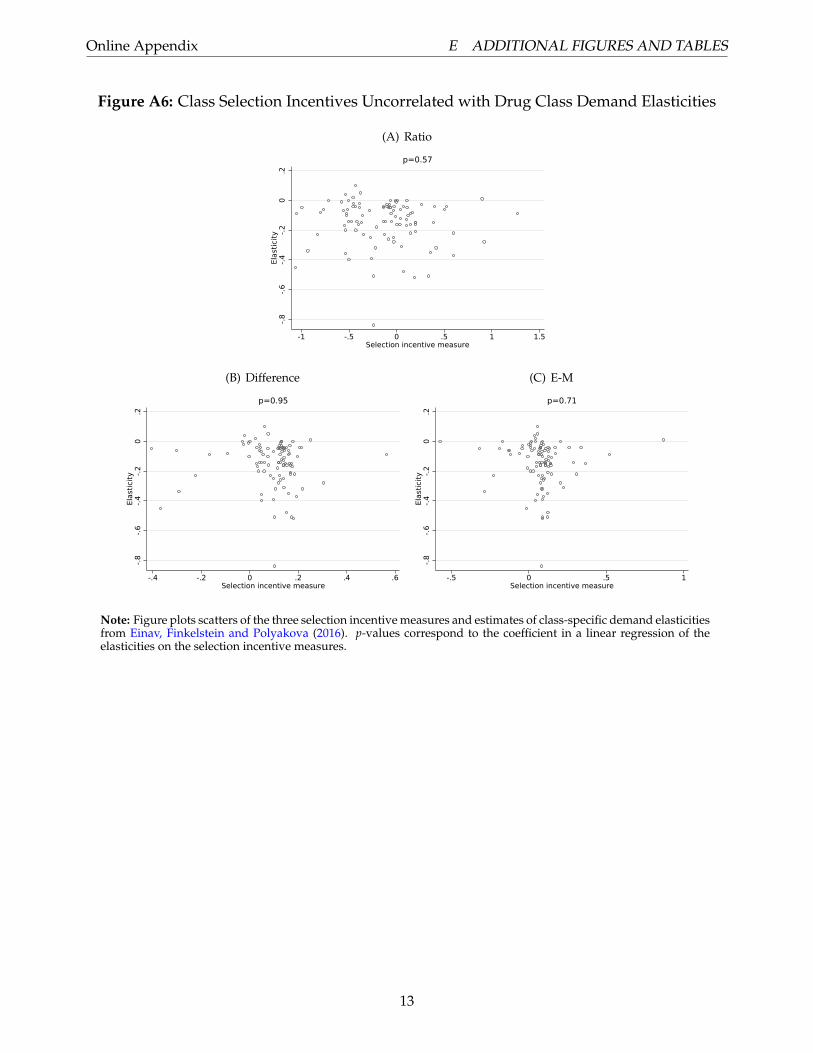
Online Appendix E ADDITIONAL FIGURES AND TABLES

Figure A6: Class Selection Incentives Uncorrelated with Drug Class Demand Elasticities

(A) Ratio

-.8-.6

-.4-.2

0.2

Elas

ticity

-1 -.5 0 .5 1 1.5Selection incentive measure

p=0.57

(B) Difference

-.8-.6

-.4-.2

0.2

Elas

ticity

-.4 -.2 0 .2 .4 .6Selection incentive measure

p=0.95

(C) E-M

-.8-.6

-.4-.2

0.2

Elas

ticity

-.5 0 .5 1Selection incentive measure

p=0.71

Note: Figure plots scatters of the three selection incentive measures and estimates of class-specific demand elasticitiesfrom Einav, Finkelstein and Polyakova (2016). p-values correspond to the coefficient in a linear regression of theelasticities on the selection incentive measures.

13

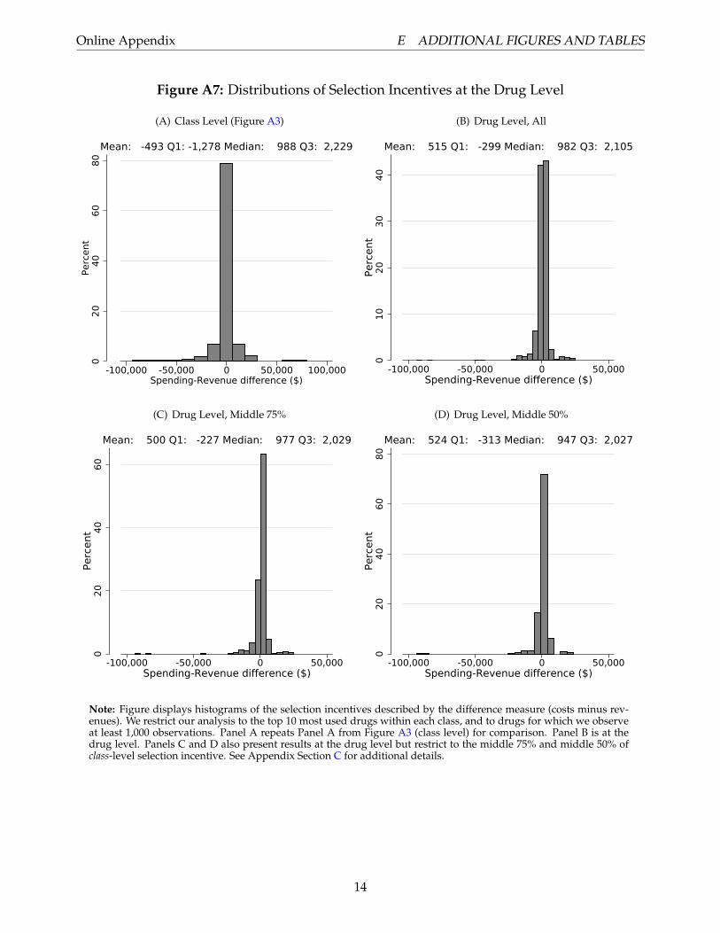
Online Appendix E ADDITIONAL FIGURES AND TABLES

Figure A7: Distributions of Selection Incentives at the Drug Level

(A) Class Level (Figure A3)

020

4060

80Pe

rcen

t

-100,000 -50,000 0 50,000 100,000Spending-Revenue difference ($)

Mean: -493 Q1: -1,278 Median: 988 Q3: 2,229

(B) Drug Level, All

010

2030

40Pe

rcen

t-100,000 -50,000 0 50,000

Spending-Revenue difference ($)

Mean: 515 Q1: -299 Median: 982 Q3: 2,105

(C) Drug Level, Middle 75%

020

4060

Perc

ent

-100,000 -50,000 0 50,000Spending-Revenue difference ($)

Mean: 500 Q1: -227 Median: 977 Q3: 2,029

(D) Drug Level, Middle 50%

020

4060

80Pe

rcen

t

-100,000 -50,000 0 50,000Spending-Revenue difference ($)

Mean: 524 Q1: -313 Median: 947 Q3: 2,027

Note: Figure displays histograms of the selection incentives described by the difference measure (costs minus rev-enues). We restrict our analysis to the top 10 most used drugs within each class, and to drugs for which we observeat least 1,000 observations. Panel A repeats Panel A from Figure A3 (class level) for comparison. Panel B is at thedrug level. Panels C and D also present results at the drug level but restrict to the middle 75% and middle 50% ofclass-level selection incentive. See Appendix Section C for additional details.

14

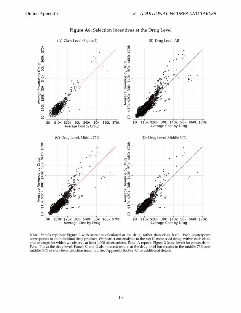
Online Appendix E ADDITIONAL FIGURES AND TABLES

Figure A8: Selection Incentives at the Drug Level

(A) Class Level (Figure 2)$0

$10k

$20k

30k

$40k

50k

$60k

$70k

Aver

age

Rev

enue

by

Gro

up

$0 $10k $20k 30k $40k 50k $60k $70kAverage Cost by Group

(B) Drug Level, All

$0$1

0k$2

0k30

k$4

0k50

k$6

0k$7

0kAv

erag

e Re

venu

e by

Dru

g$0 $10k $20k 30k $40k 50k $60k $70k

Average Cost by Drug

(C) Drug Level, Middle 75%

$0$1

0k$2

0k30

k$4

0k50

k$6

0k$7

0kAv

erag

e Re

venu

e by

Dru

g

$0 $10k $20k 30k $40k 50k $60k $70kAverage Cost by Drug

(D) Drug Level, Middle 50%

$0$1

0k$2

0k30

k$4

0k50

k$6

0k$7

0kAv

erag

e Re

venu

e by

Dru

g

$0 $10k $20k 30k $40k 50k $60k $70kAverage Cost by Drug

Note: Panels replicate Figure 2 with statistics calculated at the drug, rather than class, level. Each scatterpointcorresponds to an individual drug product. We restrict our analysis to the top 10 most used drugs within each class,and to drugs for which we observe at least 1,000 observations. Panel A repeats Figure 2 (class level) for comparison.Panel B is at the drug level. Panels C and D also present results at the drug level but restrict to the middle 75% andmiddle 50% of class-level selection incentive. See Appendix Section C for additional details.

15

Online Appendix E ADDITIONAL FIGURES AND TABLES

Figure A9: Selection Incentives, AHFS Classification

020

000

4000

060

000

8000

0Av

erag

e to

tal s

pend

ing

($)

0 20000 40000 60000 80000Average simulated revenue ($)

Note: Figure plots the relationship between healthcare spending and simulated revenue for each therapeutic classof drugs, as in Figure 2. Here, drugs are re-organized from REDBOOK classes into classes based on the AHFSclassification. Blue circles indicate the classes for which Einav, Finkelstein and Polyakova (2016) estimate a demandelasticity that we can import to our analysis. See Figure 2 for additional notes.

16

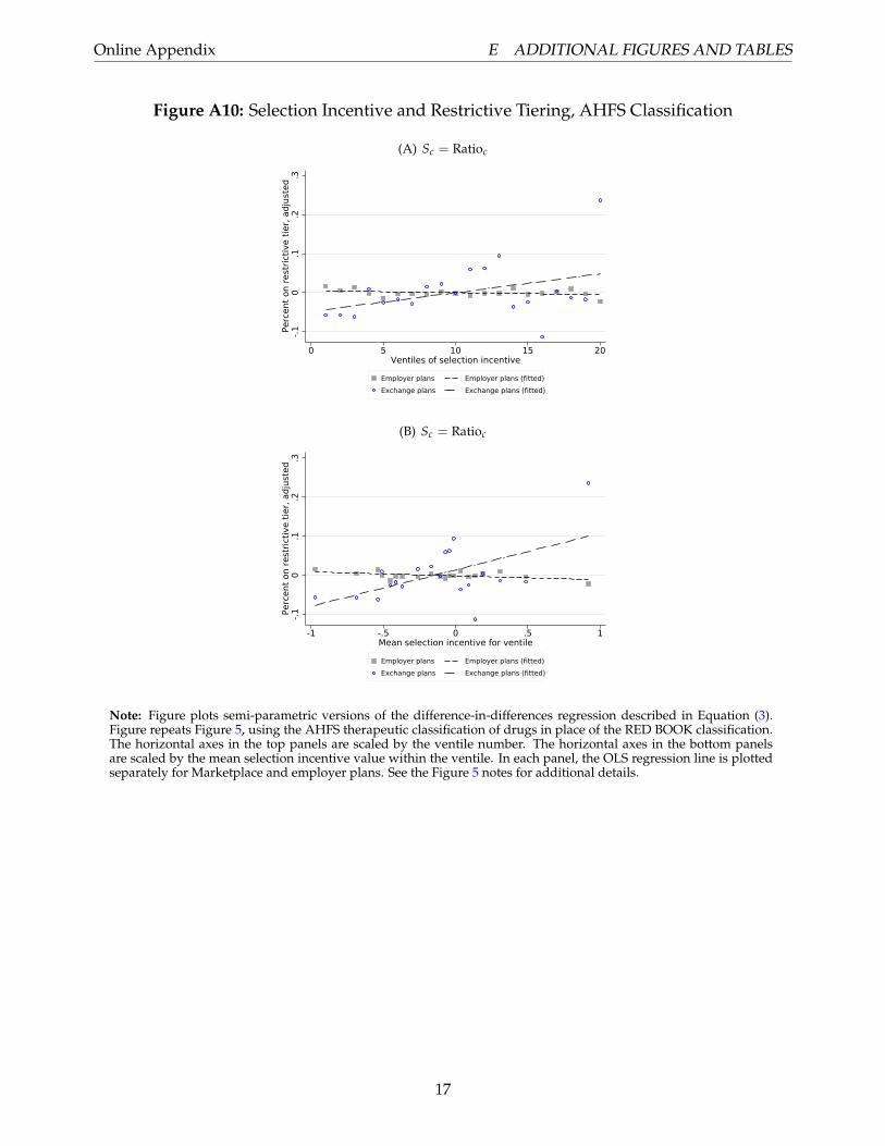
Online Appendix E ADDITIONAL FIGURES AND TABLES

Figure A10: Selection Incentive and Restrictive Tiering, AHFS Classification

(A) Sc = Ratioc

-.10

.1.2

.3Pe

rcen

t on

rest

rictiv

e tie

r, ad

just

ed

0 5 10 15 20Ventiles of selection incentive

Employer plans Employer plans (fitted)Exchange plans Exchange plans (fitted)

(B) Sc = Ratioc

-.10

.1.2

.3Pe

rcen

t on

rest

rictiv

e tie

r, ad

just

ed

-1 -.5 0 .5 1Mean selection incentive for ventile

Employer plans Employer plans (fitted)Exchange plans Exchange plans (fitted)

Note: Figure plots semi-parametric versions of the difference-in-differences regression described in Equation (3).Figure repeats Figure 5, using the AHFS therapeutic classification of drugs in place of the RED BOOK classification.The horizontal axes in the top panels are scaled by the ventile number. The horizontal axes in the bottom panelsare scaled by the mean selection incentive value within the ventile. In each panel, the OLS regression line is plottedseparately for Marketplace and employer plans. See the Figure 5 notes for additional details.

17

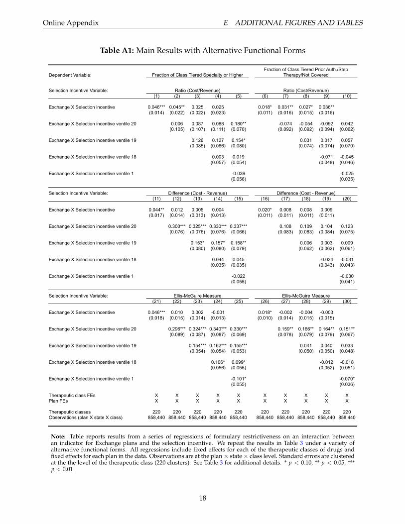
Online Appendix E ADDITIONAL FIGURES AND TABLES

Table A1: Main Results with Alternative Functional Forms

Dependent Variable:

Selection Incentive Variable:(1) (2) (3) (4) (5) (6) (7) (8) (9) (10)

Exchange X Selection incentive 0.046*** 0.045** 0.025 0.025 0.018* 0.031** 0.027* 0.036**(0.014) (0.022) (0.022) (0.023) (0.011) (0.016) (0.015) (0.016)

Exchange X Selection incentive ventile 20 0.006 0.087 0.088 0.180** -0.074 -0.054 -0.092 0.042(0.105) (0.107) (0.111) (0.070) (0.092) (0.092) (0.094) (0.062)

Exchange X Selection incentive ventile 19 0.126 0.127 0.154* 0.031 0.017 0.057(0.085) (0.086) (0.080) (0.074) (0.074) (0.070)

Exchange X Selection incentive ventile 18 0.003 0.019 -0.071 -0.045(0.057) (0.054) (0.048) (0.046)

Exchange X Selection incentive ventile 1 -0.039 -0.025(0.056) (0.035)

Selection Incentive Variable:(11) (12) (13) (14) (15) (16) (17) (18) (19) (20)

Exchange X Selection incentive 0.044** 0.012 0.005 0.004 0.020* 0.008 0.008 0.009(0.017) (0.014) (0.013) (0.013) (0.011) (0.011) (0.011) (0.011)

Exchange X Selection incentive ventile 20 0.300*** 0.325*** 0.330*** 0.337*** 0.108 0.109 0.104 0.123(0.076) (0.076) (0.076) (0.066) (0.083) (0.083) (0.084) (0.075)

Exchange X Selection incentive ventile 19 0.153* 0.157* 0.158** 0.006 0.003 0.009(0.080) (0.080) (0.079) (0.062) (0.062) (0.061)

Exchange X Selection incentive ventile 18 0.044 0.045 -0.034 -0.031(0.035) (0.035) (0.043) (0.043)

Exchange X Selection incentive ventile 1 -0.022 -0.030(0.055) (0.041)

Selection Incentive Variable:(21) (22) (23) (24) (25) (26) (27) (28) (29) (30)

Exchange X Selection incentive 0.046*** 0.010 0.002 -0.001 0.018* -0.002 -0.004 -0.003(0.018) (0.015) (0.014) (0.013) (0.010) (0.014) (0.015) (0.015)

Exchange X Selection incentive ventile 20 0.296*** 0.324*** 0.340*** 0.330*** 0.159** 0.166** 0.164** 0.151**(0.089) (0.087) (0.087) (0.069) (0.078) (0.079) (0.079) (0.067)

Exchange X Selection incentive ventile 19 0.154*** 0.162*** 0.155*** 0.041 0.040 0.033(0.054) (0.054) (0.053) (0.050) (0.050) (0.048)

Exchange X Selection incentive ventile 18 0.106* 0.099* -0.012 -0.018(0.056) (0.055) (0.052) (0.051)

Exchange X Selection incentive ventile 1 -0.101* -0.070*(0.055) (0.036)

Therapeutic class FEs X X X X X X X X X XPlan FEs X X X X X X X X X X

Therapeutic classes 220 220 220 220 220 220 220 220 220 220Observations (plan X state X class) 858,440 858,440 858,440 858,440 858,440 858,440 858,440 858,440 858,440 858,440

Ellis-McGuire Measure Ellis-McGuire Measure

Fraction of Class Tiered Specialty or HigherFraction of Class Tiered Prior Auth./Step

Therapy/Not Covered

Ratio (Cost/Revenue) Ratio (Cost/Revenue)

Difference (Cost - Revenue) Difference (Cost - Revenue)

Note: Table reports results from a series of regressions of formulary restrictiveness on an interaction betweenan indicator for Exchange plans and the selection incentive. We repeat the results in Table 3 under a variety ofalternative functional forms. All regressions include fixed effects for each of the therapeutic classes of drugs andfixed effects for each plan in the data. Observations are at the plan× state× class level. Standard errors are clusteredat the the level of the therapeutic class (220 clusters). See Table 3 for additional details. * p < 0.10, ** p < 0.05, ***p < 0.01

18

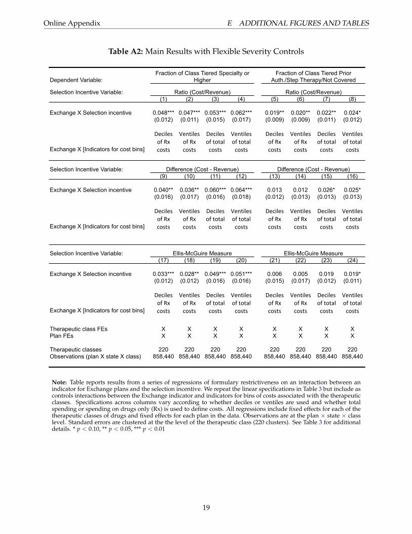
Online Appendix E ADDITIONAL FIGURES AND TABLES

Table A2: Main Results with Flexible Severity Controls

Dependent Variable:

Selection Incentive Variable:(1) (2) (3) (4) (5) (6) (7) (8)

Exchange X Selection incentive 0.048*** 0.047*** 0.053*** 0.062*** 0.019** 0.020** 0.022** 0.024*(0.012) (0.011) (0.015) (0.017) (0.009) (0.009) (0.011) (0.012)

Exchange X [Indicators for cost bins]

DecilesofRxcosts

VentilesofRxcosts

Decilesoftotalcosts

Ventilesoftotalcosts

DecilesofRxcosts

VentilesofRxcosts

Decilesoftotalcosts

Ventilesoftotalcosts

Selection Incentive Variable:(9) (10) (11) (12) (13) (14) (15) (16)

Exchange X Selection incentive 0.040** 0.036** 0.060*** 0.064*** 0.013 0.012 0.026* 0.025*(0.016) (0.017) (0.016) (0.018) (0.012) (0.013) (0.013) (0.013)

Exchange X [Indicators for cost bins]

DecilesofRxcosts

VentilesofRxcosts

Decilesoftotalcosts

Ventilesoftotalcosts

DecilesofRxcosts

VentilesofRxcosts

Decilesoftotalcosts

Ventilesoftotalcosts

Selection Incentive Variable:(17) (18) (19) (20) (21) (22) (23) (24)

Exchange X Selection incentive 0.033*** 0.028** 0.049*** 0.051*** 0.006 0.005 0.019 0.019*(0.012) (0.012) (0.016) (0.016) (0.015) (0.017) (0.012) (0.011)

Exchange X [Indicators for cost bins]

DecilesofRxcosts

VentilesofRxcosts

Decilesoftotalcosts

Ventilesoftotalcosts

DecilesofRxcosts

VentilesofRxcosts

Decilesoftotalcosts

Ventilesoftotalcosts

Therapeutic class FEs X X X X X X X XPlan FEs X X X X X X X X

Therapeutic classes 220 220 220 220 220 220 220 220Observations (plan X state X class) 858,440 858,440 858,440 858,440 858,440 858,440 858,440 858,440

Ellis-McGuire Measure Ellis-McGuire Measure

Fraction of Class Tiered Specialty or Higher

Fraction of Class Tiered Prior Auth./Step Therapy/Not Covered

Ratio (Cost/Revenue) Ratio (Cost/Revenue)

Difference (Cost - Revenue) Difference (Cost - Revenue)

Note: Table reports results from a series of regressions of formulary restrictiveness on an interaction between anindicator for Exchange plans and the selection incentive. We repeat the linear specifications in Table 3 but include ascontrols interactions between the Exchange indicator and indicators for bins of costs associated with the therapeuticclasses. Specifications across columns vary according to whether deciles or ventiles are used and whether totalspending or spending on drugs only (Rx) is used to define costs. All regressions include fixed effects for each of thetherapeutic classes of drugs and fixed effects for each plan in the data. Observations are at the plan × state × classlevel. Standard errors are clustered at the the level of the therapeutic class (220 clusters). See Table 3 for additionaldetails. * p < 0.10, ** p < 0.05, *** p < 0.01

19

Online Appendix E ADDITIONAL FIGURES AND TABLES

Table A3: Additional Summary Statistics: Generic and Branded Tiering Separately

Employer Plans

Exchange Plans

Employer Plans

Exchange Plans

(1) (2) (3) (4)

Non-Retrictive Tiers Total: 0.56 0.30 0.60 0.61Generic preferred 0.00 0.00 0.60 0.48Generic 0.00 0.00 0.00 0.13Preferred brand 0.12 0.08 0.00 0.00Covered/ Non-preferred brand 0.44 0.22 0.00 0.00

Restrictive Tiers Total: 0.44 0.70 0.40 0.39Specialty 0.00 0.01 0.00 0.00Not listed 0.33 0.28 0.34 0.24Medical 0.00 0.01 0.00 0.00Prior Authorization/Step (PA/ST) 0.01 0.15 0.00 0.03Not covered 0.10 0.25 0.06 0.11

Therapeutic Classes 218 218 192 192

Branded Drugs Only Generic Drugs Only

Note: Table lists formulary statistics separately for self-insured employer and Exchange plans. Tiers are listed fromtop to bottom in order of increasing restrictiveness, though the Prior Authorization/Step Therapy (PA/ST) tier ishorizontally differentiated by imposing non-price hurdles to access. See notes to Table 1 for additional detail.

20

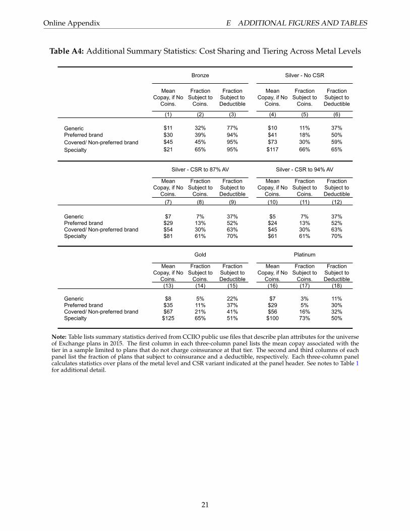
Online Appendix E ADDITIONAL FIGURES AND TABLES

Table A4: Additional Summary Statistics: Cost Sharing and Tiering Across Metal Levels

Mean Copay, if No

Coins.

Fraction Subject to

Coins.

Fraction Subject to Deductible

Mean Copay, if No

Coins.

Fraction Subject to

Coins.

Fraction Subject to Deductible

(1) (2) (3) (4) (5) (6)

Generic $11 32% 77% $10 11% 37%Preferred brand $30 39% 94% $41 18% 50%Covered/ Non-preferred brand $45 45% 95% $73 30% 59%Specialty $21 65% 95% $117 66% 65%

Mean Copay, if No

Coins.

Fraction Subject to

Coins.

Fraction Subject to Deductible

Mean Copay, if No

Coins.

Fraction Subject to

Coins.

Fraction Subject to Deductible

(7) (8) (9) (10) (11) (12)

Generic $7 7% 37% $5 7% 37%Preferred brand $29 13% 52% $24 13% 52%Covered/ Non-preferred brand $54 30% 63% $45 30% 63%Specialty $81 61% 70% $61 61% 70%

Mean Copay, if No

Coins.

Fraction Subject to

Coins.

Fraction Subject to Deductible

Mean Copay, if No

Coins.

Fraction Subject to

Coins.

Fraction Subject to Deductible

(13) (14) (15) (16) (17) (18)

Generic $8 5% 22% $7 3% 11%Preferred brand $35 11% 37% $29 5% 30%Covered/ Non-preferred brand $67 21% 41% $56 16% 32%Specialty $125 65% 51% $100 73% 50%

Silver - CSR to 87% AV Silver - CSR to 94% AV

Gold Platinum

Bronze Silver - No CSR

Note: Table lists summary statistics derived from CCIIO public use files that describe plan attributes for the universeof Exchange plans in 2015. The first column in each three-column panel lists the mean copay associated with thetier in a sample limited to plans that do not charge coinsurance at that tier. The second and third columns of eachpanel list the fraction of plans that subject to coinsurance and a deductible, respectively. Each three-column panelcalculates statistics over plans of the metal level and CSR variant indicated at the panel header. See notes to Table 1for additional detail.

21

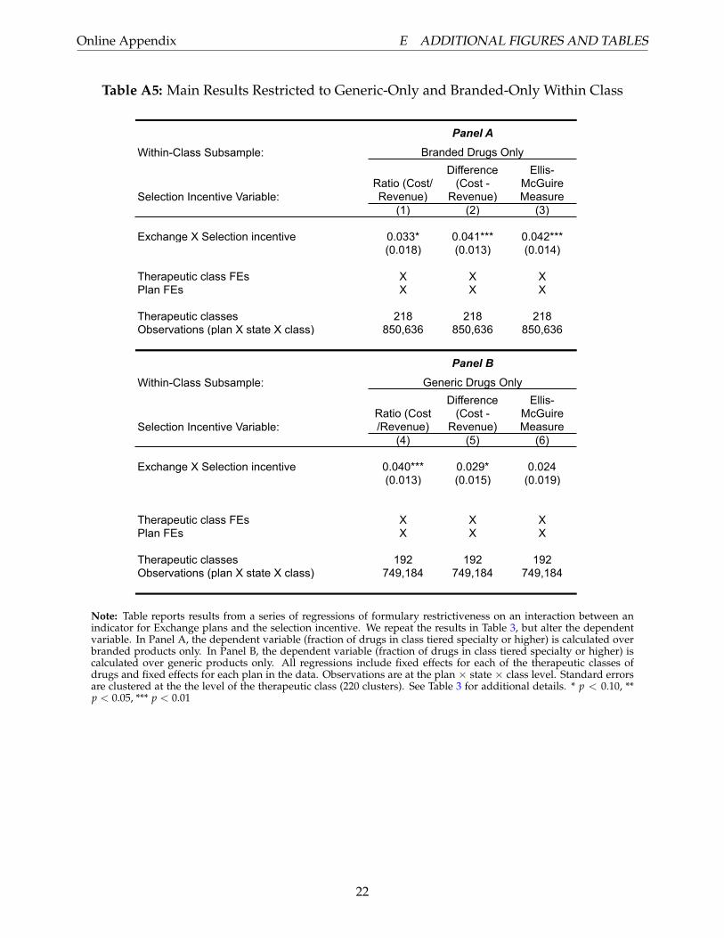
Online Appendix E ADDITIONAL FIGURES AND TABLES

Table A5: Main Results Restricted to Generic-Only and Branded-Only Within Class

Within-Class Subsample:

Selection Incentive Variable:Ratio (Cost/ Revenue)

Difference (Cost -

Revenue)

Ellis-McGuire Measure

(1) (2) (3)

Exchange X Selection incentive 0.033* 0.041*** 0.042***(0.018) (0.013) (0.014)

Therapeutic class FEs X X XPlan FEs X X X

Therapeutic classes 218 218 218Observations (plan X state X class) 850,636 850,636 850,636

Within-Class Subsample:

Selection Incentive Variable:Ratio (Cost /Revenue)

Difference (Cost -

Revenue)

Ellis-McGuire Measure

(4) (5) (6)

Exchange X Selection incentive 0.040*** 0.029* 0.024(0.013) (0.015) (0.019)

Therapeutic class FEs X X XPlan FEs X X X

Therapeutic classes 192 192 192Observations (plan X state X class) 749,184 749,184 749,184

Panel ABranded Drugs Only

Panel BGeneric Drugs Only

Note: Table reports results from a series of regressions of formulary restrictiveness on an interaction between anindicator for Exchange plans and the selection incentive. We repeat the results in Table 3, but alter the dependentvariable. In Panel A, the dependent variable (fraction of drugs in class tiered specialty or higher) is calculated overbranded products only. In Panel B, the dependent variable (fraction of drugs in class tiered specialty or higher) iscalculated over generic products only. All regressions include fixed effects for each of the therapeutic classes ofdrugs and fixed effects for each plan in the data. Observations are at the plan × state × class level. Standard errorsare clustered at the the level of the therapeutic class (220 clusters). See Table 3 for additional details. * p < 0.10, **p < 0.05, *** p < 0.01

22

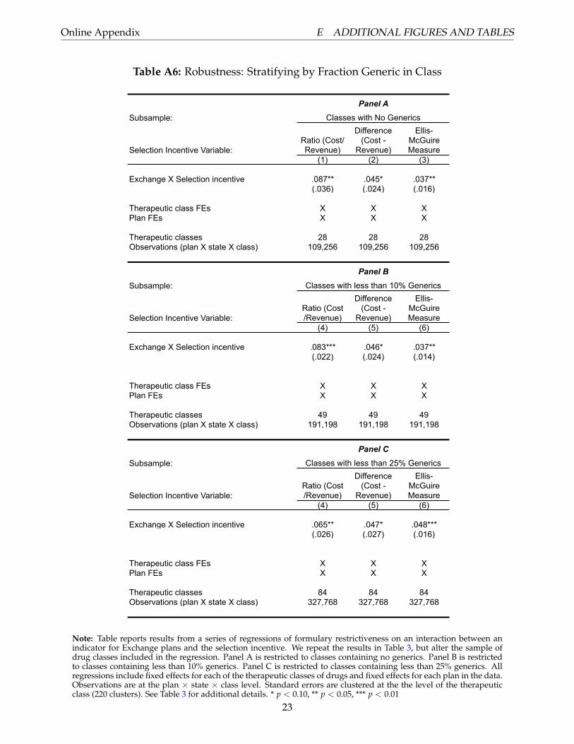
Online Appendix E ADDITIONAL FIGURES AND TABLES

Table A6: Robustness: Stratifying by Fraction Generic in Class

Subsample:

Selection Incentive Variable:Ratio (Cost/ Revenue)

Difference (Cost -

Revenue)

Ellis-McGuire Measure

(1) (2) (3)

Exchange X Selection incentive .087** .045* .037**(.036) (.024) (.016)

Therapeutic class FEs X X XPlan FEs X X X

Therapeutic classes 28 28 28Observations (plan X state X class) 109,256 109,256 109,256

Subsample:

Selection Incentive Variable:Ratio (Cost /Revenue)

Difference (Cost -

Revenue)

Ellis-McGuire Measure

(4) (5) (6)

Exchange X Selection incentive .083*** .046* .037**(.022) (.024) (.014)

Therapeutic class FEs X X XPlan FEs X X X

Therapeutic classes 49 49 49Observations (plan X state X class) 191,198 191,198 191,198

Subsample:

Selection Incentive Variable:Ratio (Cost /Revenue)

Difference (Cost -

Revenue)

Ellis-McGuire Measure

(4) (5) (6)

Exchange X Selection incentive .065** .047* .048***(.026) (.027) (.016)

Therapeutic class FEs X X XPlan FEs X X X

Therapeutic classes 84 84 84Observations (plan X state X class) 327,768 327,768 327,768

Panel AClasses with No Generics

Panel BClasses with less than 10% Generics

Classes with less than 25% Generics

Panel C

Note: Table reports results from a series of regressions of formulary restrictiveness on an interaction between anindicator for Exchange plans and the selection incentive. We repeat the results in Table 3, but alter the sample ofdrug classes included in the regression. Panel A is restricted to classes containing no generics. Panel B is restrictedto classes containing less than 10% generics. Panel C is restricted to classes containing less than 25% generics. Allregressions include fixed effects for each of the therapeutic classes of drugs and fixed effects for each plan in the data.Observations are at the plan × state × class level. Standard errors are clustered at the the level of the therapeuticclass (220 clusters). See Table 3 for additional details. * p < 0.10, ** p < 0.05, *** p < 0.01

23

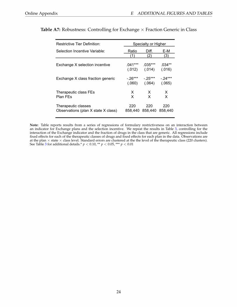
Online Appendix E ADDITIONAL FIGURES AND TABLES

Table A7: Robustness: Controlling for Exchange × Fraction Generic in Class

Restrictive Tier Definition:

Selection Incentive Variable: Ratio Diff. E-M(1) (2) (3)

Exchange X selection incentive .041*** .035*** .034**(.012) (.014) (.016)

Exchange X class fraction generic -.26*** -.25*** -.24***(.060) (.064) (.065)

Therapeutic class FEs X X XPlan FEs X X X

Therapeutic classes 220 220 220Observations (plan X state X class) 858,440 858,440 858,440

Specialty or Higher

Note: Table reports results from a series of regressions of formulary restrictiveness on an interaction betweenan indicator for Exchange plans and the selection incentive. We repeat the results in Table 3, controlling for theinteraction of the Exchange indicator and the fraction of drugs in the class that are generic. All regressions includefixed effects for each of the therapeutic classes of drugs and fixed effects for each plan in the data. Observations areat the plan × state × class level. Standard errors are clustered at the the level of the therapeutic class (220 clusters).See Table 3 for additional details.* p < 0.10, ** p < 0.05, *** p < 0.01

24

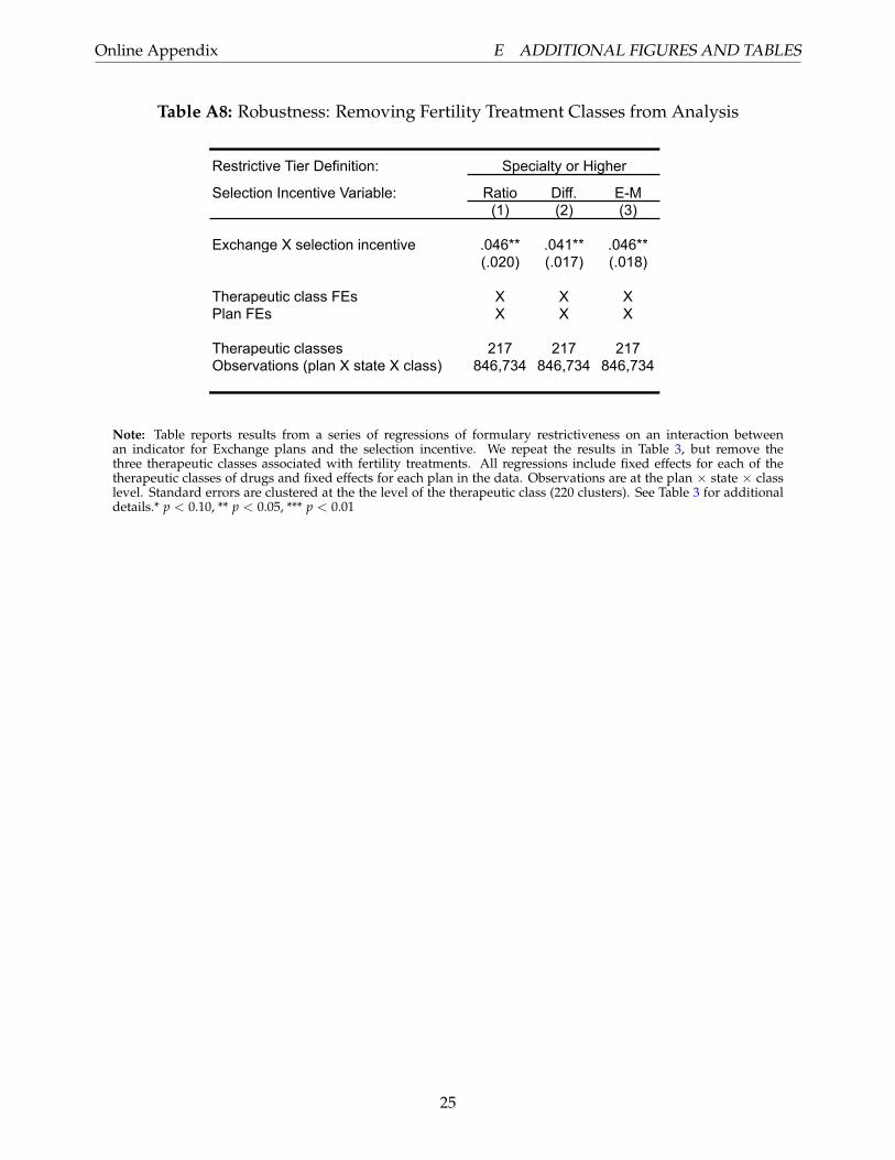
Online Appendix E ADDITIONAL FIGURES AND TABLES

Table A8: Robustness: Removing Fertility Treatment Classes from Analysis

Restrictive Tier Definition:

Selection Incentive Variable: Ratio Diff. E-M(1) (2) (3)

Exchange X selection incentive .046** .041** .046**(.020) (.017) (.018)

Therapeutic class FEs X X XPlan FEs X X X

Therapeutic classes 217 217 217Observations (plan X state X class) 846,734 846,734 846,734

Specialty or Higher

Note: Table reports results from a series of regressions of formulary restrictiveness on an interaction betweenan indicator for Exchange plans and the selection incentive. We repeat the results in Table 3, but remove thethree therapeutic classes associated with fertility treatments. All regressions include fixed effects for each of thetherapeutic classes of drugs and fixed effects for each plan in the data. Observations are at the plan × state × classlevel. Standard errors are clustered at the the level of the therapeutic class (220 clusters). See Table 3 for additionaldetails.* p < 0.10, ** p < 0.05, *** p < 0.01

25

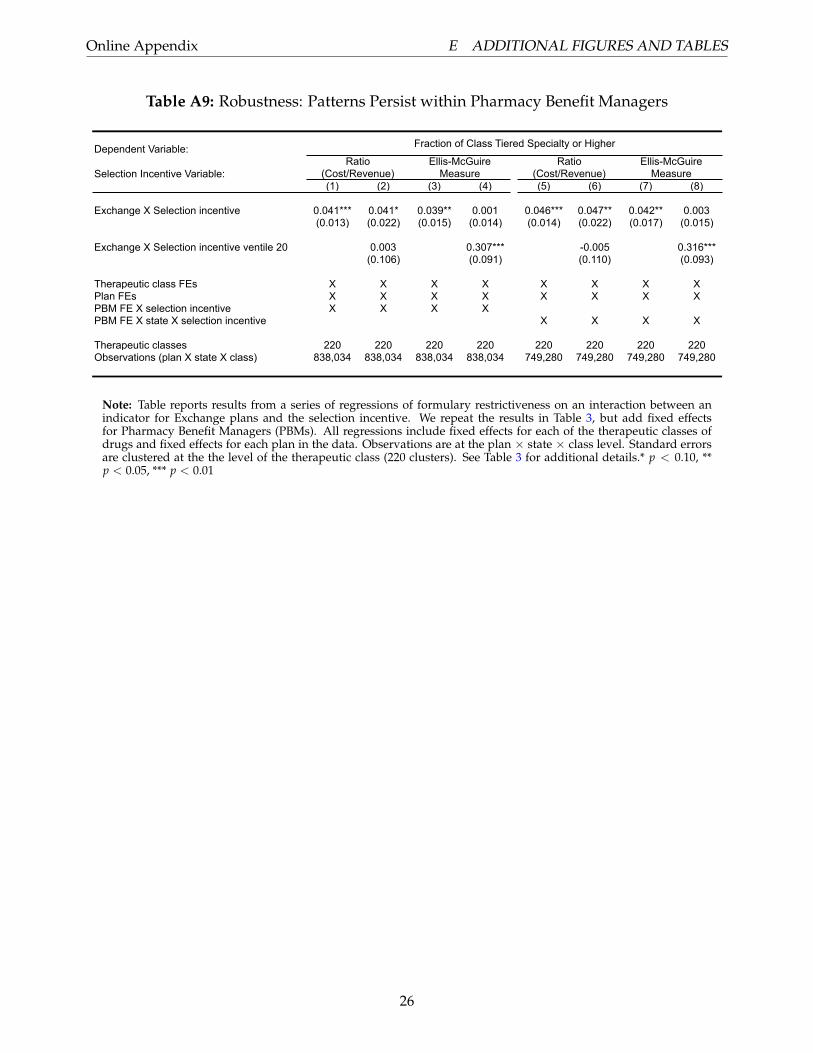
Online Appendix E ADDITIONAL FIGURES AND TABLES

Table A9: Robustness: Patterns Persist within Pharmacy Benefit Managers

Dependent Variable:

Selection Incentive Variable:(1) (2) (3) (4) (5) (6) (7) (8)

Exchange X Selection incentive 0.041*** 0.041* 0.039** 0.001 0.046*** 0.047** 0.042** 0.003(0.013) (0.022) (0.015) (0.014) (0.014) (0.022) (0.017) (0.015)

Exchange X Selection incentive ventile 20 0.003 0.307*** -0.005 0.316***(0.106) (0.091) (0.110) (0.093)

Therapeutic class FEs X X X X X X X XPlan FEs X X X X X X X XPBM FE X selection incentive X X X XPBM FE X state X selection incentive X X X X

Therapeutic classes 220 220 220 220 220 220 220 220Observations (plan X state X class) 838,034 838,034 838,034 838,034 749,280 749,280 749,280 749,280

Ellis-McGuire Measure

Ratio (Cost/Revenue)

Ellis-McGuire Measure

Ratio (Cost/Revenue)

Fraction of Class Tiered Specialty or Higher

Note: Table reports results from a series of regressions of formulary restrictiveness on an interaction between anindicator for Exchange plans and the selection incentive. We repeat the results in Table 3, but add fixed effectsfor Pharmacy Benefit Managers (PBMs). All regressions include fixed effects for each of the therapeutic classes ofdrugs and fixed effects for each plan in the data. Observations are at the plan × state × class level. Standard errorsare clustered at the the level of the therapeutic class (220 clusters). See Table 3 for additional details.* p < 0.10, **p < 0.05, *** p < 0.01

26

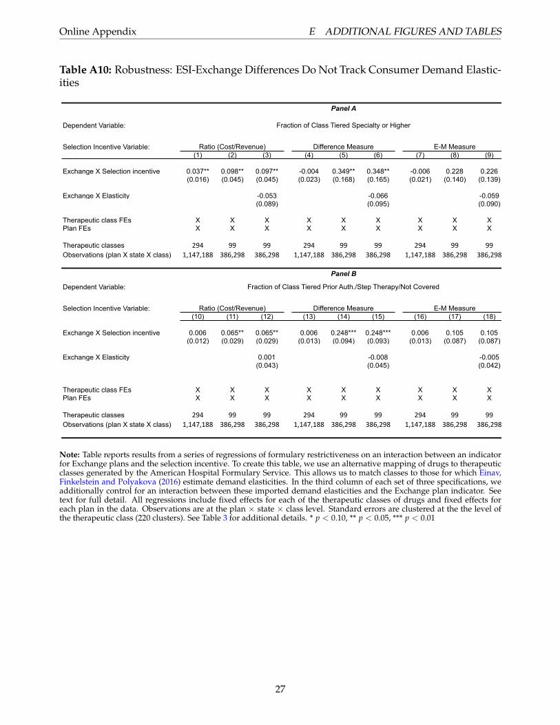
Online Appendix E ADDITIONAL FIGURES AND TABLES

Table A10: Robustness: ESI-Exchange Differences Do Not Track Consumer Demand Elastic-ities

Dependent Variable:

Selection Incentive Variable:(1) (2) (3) (4) (5) (6) (7) (8) (9)

Exchange X Selection incentive 0.037** 0.098** 0.097** -0.004 0.349** 0.348** -0.006 0.228 0.226(0.016) (0.045) (0.045) (0.023) (0.168) (0.165) (0.021) (0.140) (0.139)

Exchange X Elasticity -0.053 -0.066 -0.059(0.089) (0.095) (0.090)

Therapeutic class FEs X X X X X X X X XPlan FEs X X X X X X X X X

Therapeutic classes 294 99 99 294 99 99 294 99 99Observations (plan X state X class) 1,147,188 386,298 386,298 1,147,188 386,298 386,298 1,147,188 386,298 386,298

Dependent Variable:

Selection Incentive Variable:(10) (11) (12) (13) (14) (15) (16) (17) (18)

Exchange X Selection incentive 0.006 0.065** 0.065** 0.006 0.248*** 0.248*** 0.006 0.105 0.105(0.012) (0.029) (0.029) (0.013) (0.094) (0.093) (0.013) (0.087) (0.087)

Exchange X Elasticity 0.001 -0.008 -0.005(0.043) (0.045) (0.042)

Therapeutic class FEs X X X X X X X X XPlan FEs X X X X X X X X X

Therapeutic classes 294 99 99 294 99 99 294 99 99Observations (plan X state X class) 1,147,188 386,298 386,298 1,147,188 386,298 386,298 1,147,188 386,298 386,298

E-M Measure

E-M Measure

Fraction of Class Tiered Specialty or Higher

Fraction of Class Tiered Prior Auth./Step Therapy/Not Covered

Panel A

Panel B

Ratio (Cost/Revenue) Difference Measure

Ratio (Cost/Revenue) Difference Measure

Note: Table reports results from a series of regressions of formulary restrictiveness on an interaction between an indicatorfor Exchange plans and the selection incentive. To create this table, we use an alternative mapping of drugs to therapeuticclasses generated by the American Hospital Formulary Service. This allows us to match classes to those for which Einav,Finkelstein and Polyakova (2016) estimate demand elasticities. In the third column of each set of three specifications, weadditionally control for an interaction between these imported demand elasticities and the Exchange plan indicator. Seetext for full detail. All regressions include fixed effects for each of the therapeutic classes of drugs and fixed effects foreach plan in the data. Observations are at the plan × state × class level. Standard errors are clustered at the the level ofthe therapeutic class (220 clusters). See Table 3 for additional details. * p < 0.10, ** p < 0.05, *** p < 0.01

27