SCOUR, FILL, AND SALMON SPAWNING

IN A NORTHERN CALIFORNIA COASTAL STREAM

by

Paul E. Bigelow

A Thesis

Presented to

The Faculty of Humboldt State University

In Partial Fulfillment

of Requirements for the Degree

Master of Science

In Geology

May 9, 2003

SCOUR, FILL, AND SALMON SPAWNING

IN A NORTHERN CALIFORNIA COASTAL STREAM

by

Paul E. Bigelow

ABSTRACT

SCOUR, FILL, AND SALMON SPAWNING

IN A NORTHERN CALIFORNIA COASTAL STREAM

by

Paul E. Bigelow

Streambed scour and fill affecting incubation survival of salmon embryos were

investigated in a Northern California coastal stream (Freshwater Creek) for coho

(Oncorhynchus kisutch) and chinook (Oncorhynchus tshawytscha) species. Objectives of

the study were to: (1) test a reach-scale scour and fill model (Haschenburger 1999) based

on Shields stress (dimensionless shear stress), and (2) test two published hypotheses of

salmon spawning adaptation to streambed scour. Testing of the model clarified some

limitations, revealed potential improvements, and demonstrated sufficient potential for

predicting scour at salmon spawning areas (redds) based on a small sample size (n = 9

redds) to warrant additional testing. The model appears best suited for individual floods

on reaches that are straight, in equilibrium between sediment supply and transport, and

have roughness elements similar to the creeks where the model was developed.

Differences in model predictions and measured values were likely due to variable scour

and fill patterns in Freshwater Creek that were weakly influenced by Shields stress and

highly influenced by sediment supply, location within the channel network, and channel

morphology (form roughness).

iii

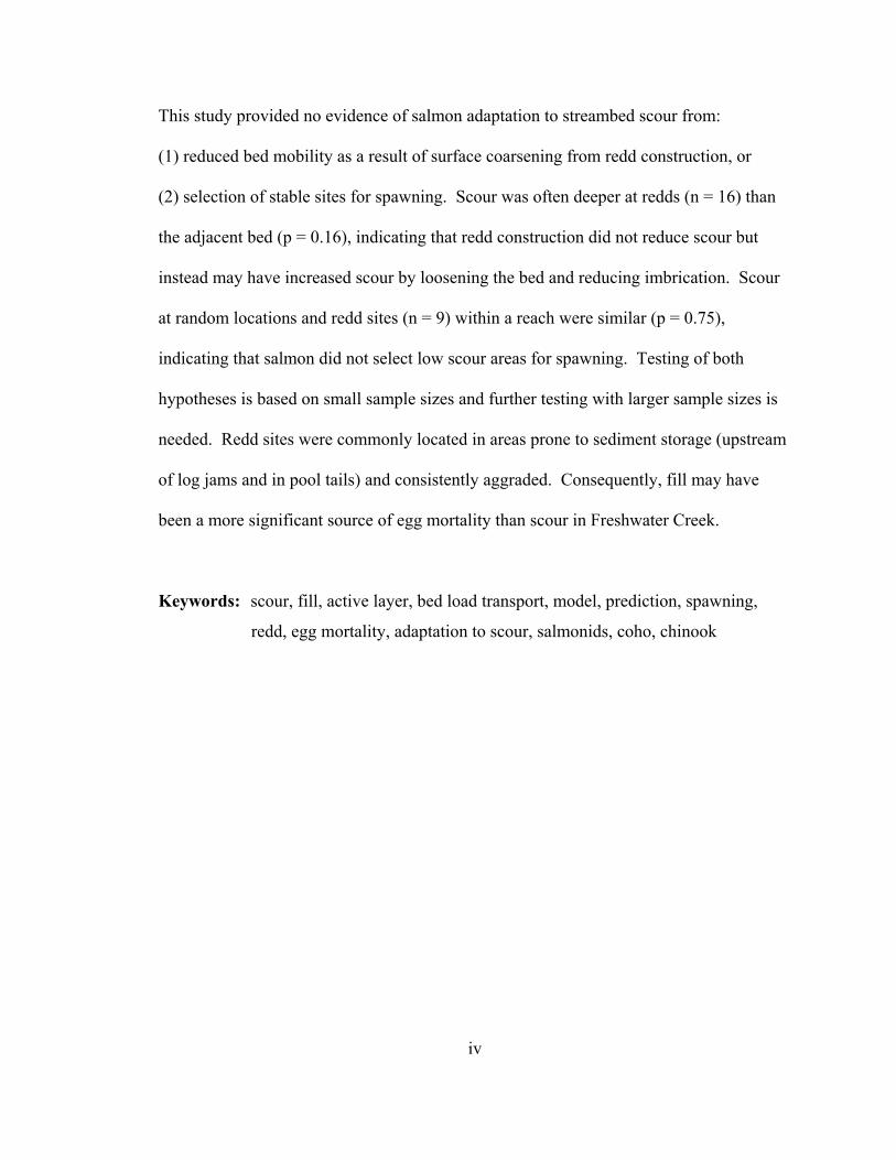
This study provided no evidence of salmon adaptation to streambed scour from:

(1) reduced bed mobility as a result of surface coarsening from redd construction, or

(2) selection of stable sites for spawning. Scour was often deeper at redds (n = 16) than

the adjacent bed (p = 0.16), indicating that redd construction did not reduce scour but

instead may have increased scour by loosening the bed and reducing imbrication. Scour

at random locations and redd sites (n = 9) within a reach were similar (p = 0.75),

indicating that salmon did not select low scour areas for spawning. Testing of both

hypotheses is based on small sample sizes and further testing with larger sample sizes is

needed. Redd sites were commonly located in areas prone to sediment storage (upstream

of log jams and in pool tails) and consistently aggraded. Consequently, fill may have

been a more significant source of egg mortality than scour in Freshwater Creek.

Keywords: scour, fill, active layer, bed load transport, model, prediction, spawning,

redd, egg mortality, adaptation to scour, salmonids, coho, chinook

iv

ACKNOWLEDGEMENTS

As with most pursuits in life, it was the people that made this thesis most worthwhile. I

wish to thank my committee members: Tom Lisle, who allowed me the independence to

discover on my own while providing tersely cogent guidance when needed; Bret Harvey,

whose sharp wit and advice kept me from “crying in my coffee”; and I am particularly

indebted to Andre Lehre for his excellent course work, and whose combined enthusiasm,

modesty, and sense of humor inspired me to take something seriously, but not take

myself seriously. Thanks also to Scott McBain, who helped me start the thesis process,

often served as an unofficial fourth committee member, and generously provided field

equipment to perform the study. My interest in fluvial geomorphology and salmon was

inspired by authentic classes and discussions with Terry Roelofs and Bill Trush.

I could not have completed the field work without the kind help and comic relief from my

friends Dave O’Rourke, Mishka Straka, Rick Rogers, and my brother Mark Bigelow.

Special recognition goes to Devin Stephens, who put in several long days of stream

surveying while wearing what appeared to be penny loafers. Kevin Andras kindly helped

with color map production. The Pacific Lumber Company generously allowed access to

their land and provided assistance with field work. Some field equipment costs were

covered by an encouraging seed grant from the Geological Society of America. This

study stands on the shoulders of previous work by Judy Haschenburger and Paul

DeVries, who both provided valuable input to this study. Finally, thanks to Lee Benda

v

for encouragement to complete this thesis while keeping me employed with stimulating

work that has rapidly broadened my view and understanding of geomorphology.

This thesis is dedicated to the memory of Ken Kesey and Allen Ginsberg, whose lives

and prose have provided a boat through a sea of permanent uncertainty.

What this country needs is sanity. Individual sanity, and all the rest will come true.

-Ken Kesey

Work like the sun Shine in your heaven See what you’ve done Come down and walk

-Allen Ginsberg

vi

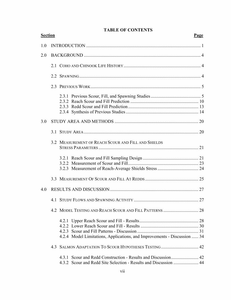
TABLE OF CONTENTS Section Page 1.0 INTRODUCTION ..................................................................................................... 1 2.0 BACKGROUND ....................................................................................................... 4 2.1 COHO AND CHINOOK LIFE HISTORY.................................................................... 4 2.2 SPAWNING........................................................................................................... 4 2.3 PREVIOUS WORK................................................................................................. 5 2.3.1 Previous Scour, Fill, and Spawning Studies ............................................ 5 2.3.2 Reach Scour and Fill Prediction ............................................................ 10 2.3.3 Redd Scour and Fill Prediction .............................................................. 13 2.3.4 Synthesis of Previous Studies ................................................................ 14 3.0 STUDY AREA AND METHODS .......................................................................... 20 3.1 STUDY AREA ..................................................................................................... 20 3.2 MEASUREMENT OF REACH SCOUR AND FILL AND SHIELDS STRESS PARAMETERS ........................................................................................ 21 3.2.1 Reach Scour and Fill Sampling Design ................................................. 21 3.2.2 Measurement of Scour and Fill.............................................................. 23 3.2.3 Measurement of Reach-Average Shields Stress .................................... 24 3.3 MEASUREMENT OF SCOUR AND FILL AT REDDS ............................................... 25 4.0 RESULTS AND DISCUSSION.............................................................................. 27 4.1 STUDY FLOWS AND SPAWNING ACTIVITY ......................................................... 27 4.2 MODEL TESTING AND REACH SCOUR AND FILL PATTERNS ............................... 28 4.2.1 Upper Reach Scour and Fill - Results.................................................... 28 4.2.2 Lower Reach Scour and Fill - Results ................................................... 30 4.2.3 Scour and Fill Patterns - Discussion ...................................................... 31 4.2.4 Model Limitations, Applications, and Improvements - Discussion ...... 34 4.3 SALMON ADAPTATION TO SCOUR HYPOTHESES TESTING................................. 42 4.3.1 Scour and Redd Construction - Results and Discussion........................ 42 4.3.2 Scour and Redd Site Selection - Results and Discussion ...................... 44

vii

TABLE OF CONTENTS (CONTINUED)

Section Page 4.4 ADDITIONAL OBSERVATIONS ............................................................................ 46 4.4.1 Fill Patterns And Salmon Spawning ...................................................... 46 4.4.2 Model Application to Redds - Results and Discussion.......................... 48 5.0 SUMMARY AND CONCLUSIONS ...................................................................... 50 REFERENCES ................................................................................................................. 55

viii

LIST OF TABLES Table Page

1 Physical characteristics and scour and fill sampling measurements of study reaches................................................................................................................... 64

2 Summary of model constants, inputs, outputs (predictions), and measured

values (for comparison). ....................................................................................... 65 3 Summary of statistical hypotheses testing results................................................. 66 4 Scour and fill depths at redds and adjacent bed (control). Values shown

are an average of two chains, except where only one redd or control chain was recovered. Redds numbered 1-9 were within the upper reach; redds numbered 10-16 were above or below the upper reach. ....................................... 67

ix

LIST OF FIGURES Figure Page

1 Diagram of typical salmon redd showing plan view (top) and cross sectional view (bottom). Adapted from Chapman (1988) and Rennie and Millar (2000). .68

2 Freshwater Creek watershed and study reach locations, Humboldt County,

California. ............................................................................................................. 69 3 Streambed cross section showing how scour, fill, and the active layer are

measured using scour chains under different conditions. ..................................... 70 4 Representative photographs of the (A) bar-dominated upper and (B) riffle-

and plane bed-dominated lower reach. ................................................................. 71 5 Topographic maps of the (A) upper and (B) lower reach showing

approximate cross section and redd locations....................................................... 72 6 Streambed cross section showing scour chain installation steps: (1) create

pilot hole with sledge hammer and drive rod, (2) remove drive rod, (3) insert smaller probe with scour chain attached and tap to bottom with hammer, (4) remove smaller probe, and (5) pull chain upward to rotate duckbill into a horizontal position, creating an anchor. ............................................................ 73

7 Discharge in Freshwater Creek from November 1, 1999 to May 30, 2000,

recorded at the Salmon Forever (2001) gauge at the bottom of the lower reach.. 74 8 Modified relative frequency histograms of measured and predicted

(A) scour, (B) fill, and (C) active layer depths for the upper and lower reach. Measured values are in bins, model predictions are shown by line. Histograms are modified by dividing the relative frequency of each bin by the bin interval (Olkin et al. 1980). P-value is the probability of similarity between measured and model predicted distributions. ......................................... 75

9 Average streambed elevation change at each cross section (left y-axis) and

low flow water surface profile (right y-axis) for the (A) upper and (B) lower reach. Bed elevation change is based on an average of six and four scour chains per cross section on the upper and lower reaches, respectively. ............... 76

10 Distribution of (A) channel geomorphic units in both reaches and mean

scour or fill depths (and 95% confidence interval) within each unit on the (B) upper reach and (C) lower reach......................................................................77

x

LIST OF FIGURES (CONTINUED) Figure Page

11 Typical cross sections of the (A) bar-dominated upper reach and (B) riffle- and plane bed-dominated lower reach. Title on each cross section denotes its distance from the bottom of the reach................................................................... 78

12 (A) Scour depths at each redd and adjacent bed (control) locations and

(B) scour, fill, and active layer depths at each redd. Redds numbered 1 - 9 were within the upper reach; redds numbered 10 - 16 were above or below the upper reach...................................................................................................... 79

13 Modified relative frequency histograms of scour or fill depths for the (A) upper

reach and (B) redd sites (9 redds, 33 to 34 chains at redd and control locations) within the upper reach. Histograms are modified by dividing the relative frequency of each bin by the bin interval (Olkin et al. 1980). P-value is the probability of similarity between distributions ..................................................... 80

14 Example of Freshwater Creek spawning area prone to aggradation from

sediment storage behind channel-spanning log jam. ............................................ 81

xi

APPENDICES Appendix Page

A Evaluation of cross section flood stage data. ........................................................ 82 B Humboldt State University Institutional Animal Care and Use Committee

protocol approval. ................................................................................................. 83 C Estimated flood recurrence intervals for Freshwater Creek based on prorating

peak discharges of nearby Jacoby Creek. ............................................................. 84 D Cross sections ....................................................................................................... 86 E Scour and fill measurements................................................................................. 94 F Redd plan maps..................................................................................................... 99 G Redd scour and fill measurements. ..................................................................... 102

xii

1

1.0 INTRODUCTION

“Everything flows, nothing stays still.”

-Heraclitus Over their life cycle, salmon and trout (salmonids) experience highest mortality rates

during the incubation period in streambed gravels that can range from 2 - 8 months,

depending on the species (Sandercock 1991). Salmonids build a redd by digging a

depression into streambed gravels, depositing and fertilizing the eggs in the depression,

and covering the eggs with gravel (Figure 1). When floods occur during incubation

periods, eggs can be lost if the streambed scour depth exceeds the egg deposition depth,

possibly lowering populations (Wales and Coots 1954; Seegrist and Gard 1972; Holtby

and Healey 1986; Erman et al. 1988). In streams with high local concentrations of fines,

scour followed by fill at redds can allow deeper infiltration of fine sediments (Lisle 1989;

Platts et al. 1989, Peterson and Quinn 1996a) and reduce dissolved oxygen supply to

embryos (see review by Chapman 1988) or form a seal within and over redds that

prevents emergence of fry (Koski 1966; Everest et al. 1987; Scrivener and Brownlee

1989).

Recent declines in Pacific salmon populations may partially reflect human impacts on

watershed conditions (Holtby and Scrivener 1989; Bisson et al. 1992). Some land-use

activities that alter the sediment flux and hydrology of rivers can increase scouring of

redds (Tripp and Poulin 1986; Nawa et al. 1990) or infiltration of fines into redds

(Mouring 1982; Platts et al. 1989; Scrivener and Brownlee 1989). Consequently, the

2

health of some salmon stocks may be sensitive to scour and fill impacts to redds

(Haschenburger 1994; DeVries 2000). A recent reach-scale scour and fill probability

model (Haschenburger 1999) is a possible candidate to predict such impacts, hereafter

referred to as the Haschenburger model. The Haschenburger model predicts a right-

skewed distribution of scour and fill depths to a first approximation using channel and

flow characteristics. While measured scour and fill distributions have been tested for

conformance with the exponential function, the specific model offered for general use has

not been validated nor has it been tested at redds.

Understanding of salmonid adaptation to streambed scour would improve application of

the Haschenburger or other scour and fill models at redds. For species that spawn during

periods of high flows, testable hypotheses of adaptation to streambed scour include:

(1) decreased bed mobility as a result of surface coarsening from redd construction

(Montgomery et al. 1996), and (2) spawning in low scour areas, such as: the top of riffles

(Yee 1981), near channel margins (Stefferud 1993), hydraulically sheltered areas behind

log jams and in side channels (Montgomery et al. 1999), and riffles and pool tails

buffered by sediment storage (DeVries 2000). Additional hypotheses that may not be

testable include depositing eggs below typical scour depths (Montgomery et al. 1996),

and natural selection for larger fish that can bury their eggs deeper or selection for fish

that spawn at times when scour is less likely (Steen and Quinn 1999). Within this

context, the objectives of this study were to:

3

1) Test the accuracy of the Haschenburger model for predicting scour and fill on a

northern California coastal stream.

2) Enhance the understanding of salmon adaptation to streambed scour by testing the

following hypotheses:

a) Redd construction reduces scour.

b) Salmon select low scour areas for spawning.

The model and hypotheses testing were performed on data collected from Freshwater

Creek in Humboldt County, California (Figure 2) during the 1999-2000 winter spawning

season for coho (Oncorhynchus kisutch) and chinook (Oncorhynchus tshawytscha)

salmon.

Because the definition of scour and fill varies between disciplines (geomorphology,

fisheries, engineering), clarification of these terms is necessary. In this study, scour is the

difference between the initial bed elevation and the deepest level of scour (or bed

mobilization) as recorded by a scour chain, fill is the net material deposited above the

deepest level of scour, and the active layer is the difference between the highest bed

elevation measured at the beginning or end of the study and the lowest level of scour (i.e.

the maximum bed elevation range at a point for a given period) (Figure 3), similar to the

“active bed” term defined by Lisle (1989). Because scour chains were only recovered

once at the end of the flood season, measurements reflect the seasonal maximum scour

and net fill depths over the study period (seasonal scour and fill).

4

2.0 BACKGROUND

The relation between scour, fill and salmon spawning has been studied by several

researchers. To provide additional context for this study, the relevant research to date

and appropriate details of salmonid life history and spawning are summarized in the

following section.

2.1 COHO AND CHINOOK LIFE HISTORY

Coho salmon generally mature after three or more years, including incubation periods of

1 to 2 months, rearing 1 or more years in freshwater, and a 1½ to 3 year growing period

in the ocean. Mature coho return to spawn in their natal streams between November and

January (California stocks) as stream temperatures decrease and rainfall and stream flow

increase, allowing coho to reach smaller low gradient tributaries with ideal spawning and

rearing conditions (Sandercock 1991). Coastal chinook salmon have a similar life

history, but can spawn in larger streams than coho and rear in freshwater for only 6 to 8

months.

2.2 SPAWNING

Spawning begins as the female turns on her side and vigorously flexes her body and tail

to dig a pit in stream gravels. The movements create a suction effect that entrains bed

materials into the current, causing gravel to deposit just below the pit and form a tailspill,

5

while fines are suspended and carried farther downstream. Cobbles too large to be

moved by the female will remain in the pit as a coarse lag (Chapman 1988; Kondolf et al.

1993). Once a pit is completed, the female pushes her anal fin between the cobbles, the

male swims alongside the female, and the eggs and milt are simultaneously deposited.

The female then resumes digging upstream to bury the first egg pocket and create another

pit. The spawning continues for several days and a single redd can contain several egg

pockets (Sandercock 1991) (Figure 1).

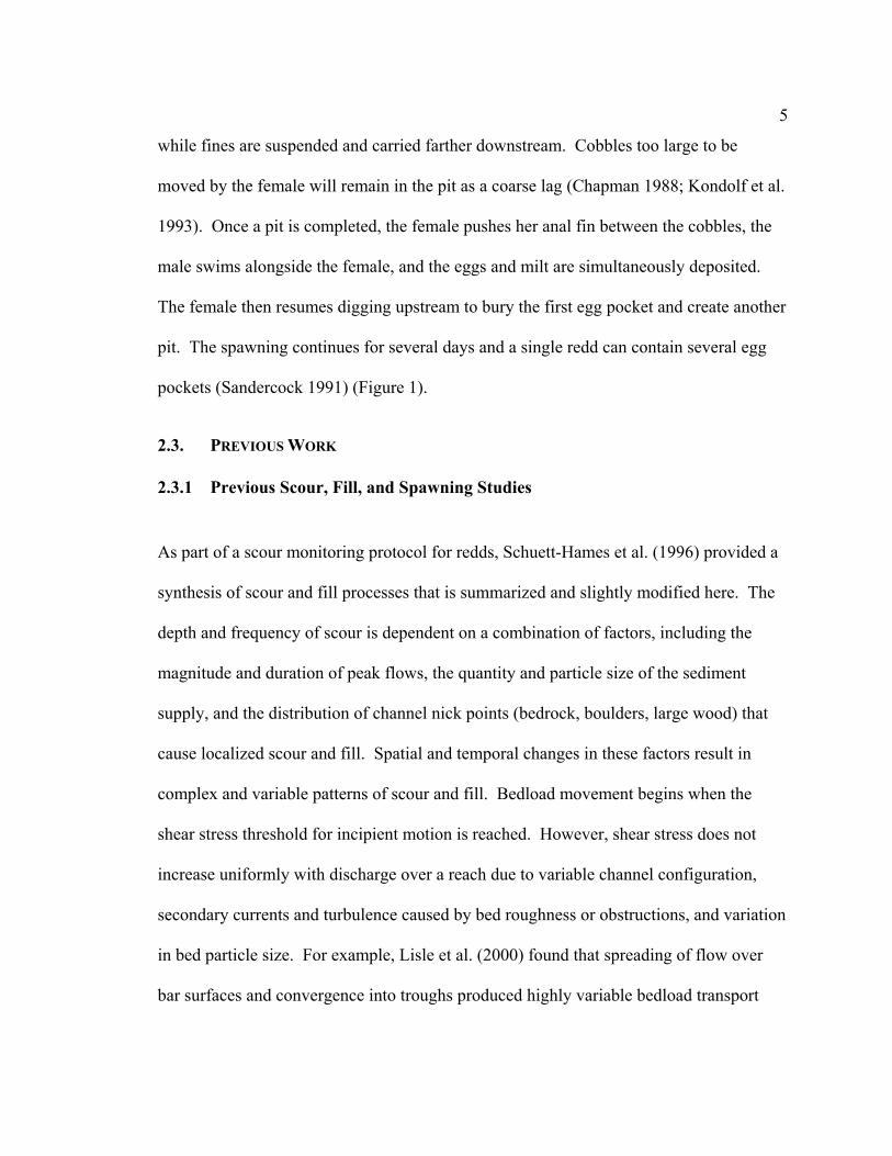
2.3. PREVIOUS WORK

2.3.1 Previous Scour, Fill, and Spawning Studies

As part of a scour monitoring protocol for redds, Schuett-Hames et al. (1996) provided a

synthesis of scour and fill processes that is summarized and slightly modified here. The

depth and frequency of scour is dependent on a combination of factors, including the

magnitude and duration of peak flows, the quantity and particle size of the sediment

supply, and the distribution of channel nick points (bedrock, boulders, large wood) that

cause localized scour and fill. Spatial and temporal changes in these factors result in

complex and variable patterns of scour and fill. Bedload movement begins when the

shear stress threshold for incipient motion is reached. However, shear stress does not

increase uniformly with discharge over a reach due to variable channel configuration,

secondary currents and turbulence caused by bed roughness or obstructions, and variation

in bed particle size. For example, Lisle et al. (2000) found that spreading of flow over

bar surfaces and convergence into troughs produced highly variable bedload transport

6

rates, and hence variable scour and fill patterns. Consequently, portions of the bed begin

to move at different thresholds and tend to occur in irregular pulses or waves (e.g. Paige

and Hickin 2000). Bed compaction that occurs during long intervals between peak flows

increases resistance to scour (e.g. Reid et al. 1985), resulting in different scour patterns

over a storm season.

DeVries (2000) also provides a synthesis of scour processes, but suggests that the size

and quantity of gravel and cobbles in a reach exert a much stronger influence on scour

depth than flood magnitude and duration. Scour and fill was measured in western

Washington streams on cross sections in relatively plane-bed, low-gradient reaches with

ample spawning gravel and cobbles. Scour occurred from (1) bedload layer movement

and (2) spatial and temporal imbalances in sediment transport rate, including (a) scour

and fill of transient finer grained deposits downstream of partial flow obstructions,

(b) scour and fill at the pool-riffle scale, where scour depth is related to distances between

riffles and the size of the riffle deposit, and (c) scour and fill at the reach scale in

response to variable sediment supplied to the reach. Scour depths from bedload layer

movement appeared to be a function of grain size and approached a limit at

approximately twice the 90th percentile of the streambed particle size distribution (2D90).

Based on the relationship between egg pocket depth and particle size (egg depth/D90

ratio) in published studies, DeVries (2000) suggests that salmonids may have adapted to

scour by burying their eggs greater than 2 to 2.5D90. In addition, salmonids may have

7

adapted to scour by constructing redds at locations in the channel least likely to

experience scour from imbalances in sediment transport rates.

Scour and fill processes and their relation to chum salmon (Oncorhynchus keta) spawning

habitat were studied extensively in Kennedy Creek near Olympia, Washington

(Montgomery et al. 1996; Schuett-Hames et. al. 1994; Schuett-Hames et al. 2000). Scour

and fill were measured in a sinuous pool-riffle reach and a relatively straight plane-bed

reach. Scour monitors were installed on cross sections in all habitat types except pool

bottoms, the only areas of the stream not used for spawning. Egg pocket depths were

also measured in redds (see Peterson and Quinn 1996b) and "auxiliary" scour monitors

were placed near egg pockets.

Scour and fill was spatially variable and approximated a right-skewed negative

exponential distribution (both reaches combined). The range of scour depth and

frequency distribution was significantly greater in the more complex pool-riffle reach due

to lateral channel migration, flow over and around large wood jams, movement of large

wood, and side channel formation. Mean scour depth was 11 centimeters (cm) (both

reaches combined), while mean scour was higher in pool lateral bars (20 cm) and pool

tails (16 cm) than in other habitat types (2 - 9 cm). The percentage of monitor locations

that scoured to 20 cm (the mean depth to measured egg pockets) was also higher in pool

lateral bars (39%) and pool tails (28%) than in other habitat types (0 - 17%). Chum

salmon appeared to favor spawning in areas with high intergravel flow and dissolved

8

oxygen levels such as pool tails. Because these areas are prone to scour at higher flows,

Schuett-Hames et al. (2000) infer that scour can be a significant source of egg loss. This

also implies that scour is not a factor in spawning site selection.

Using the same data set, Montgomery et al. (1996) speculated that the close

correspondence between egg burial and scour depths indicates an adaptation to typical

depths of scour. Based on paired pebble counts in the tailspills of redds and unspawned

adjacent areas of Kennedy Creek, spawning increased the median surface particle size by

33 to 39%. Theoretical calculations indicated that the spawning-related bed

modifications may reduce scour in redds by coarsening the surface and increasing friction

angles. In potential contradiction, Schuett-Hames et al. (1994) reported that scour in the

auxiliary egg pocket monitors was "similar or somewhat higher than on cross-sections

for the same habitat type", but cautioned that the comparison may not be appropriate

because egg pocket monitors were typically near the thalweg, while the cross section

monitors were at uniform intervals across the channel width.

In a similar study, scour and fill was measured in four chum salmon redds and adjacent

bed material in Kanaka Creek near Vancouver, British Columbia (Rennie 1998; Rennie

and Millar 2000). Scour monitors were installed on a grid over a low gradient riffle and

recovered multiple times over a single flood season. Scour depths were spatially variable

(mean = 8.5 cm) and the lack of spatial autocorrelation between scour monitors suggested

a random pattern of scour. However, localized scour and fill was noted around a rootwad

9

and near a collapsed bank. The distribution of scour depths was right skewed and

resembled a negative exponential function. Maximum scour depth at the egg pockets of

redds (mean = 6 cm, n = 4 redds) was not significantly different from the adjacent bed

(mean = 8 cm, n = 18). Rennie (1998) concluded that redd construction may not reduce

scour, however, the small sample size "limits the generality of the results".

Yee (1981) measured scour and fill in Prairie Creek, a low gradient gravel-bed coastal

stream in old growth redwood (Sequoia sempervirens) forests of northern California.

Scour chains were installed on a grid in spawning riffles and recovered multiple times

over a two-year period. Similar patterns of scour and fill were observed over the period,

where scour depths were much deeper at the bottom of the riffle (6 - 24 cm) than the head

of the riffle (3 - 8 cm). Laterally, scour and fill depths were shallow near the banks and

deeper near the thalweg. Based on the longitudinal pattern of riffle scour observed, Yee

(1981) hypothesized that salmonids have evolved to spawn at the head of riffles (pool

tails) not only for favorable intergravel flow, but also for stable gravels.

Lisle (1989) measured the infiltration of fine sediment into streambed gravel and scour

and fill of spawning areas in low-gradient northern California coastal streams over a 2 - 4

year period. Gravel filled cans (to collect fine sediment) and scour chains were installed

on cross sections in spawning areas of each stream. Fine sediment infiltrated down to the

bottom of gravel cans during small storms, but formed a seal near the top several

centimeters during larger storms. Although depth of scour and fill was highly variable,

10

the cross sections maintained the same general shape from storm to storm even though

segments of cross sections commonly scoured up to 10 cm or more during a storm. Lisle

(1989) concluded that while both scour and infiltration of fines pose a threat to incubating

eggs, scour and fill depths and rates of fine sediment infiltration are highly variable in

space and time and this "variability poses the greatest challenge to predictions of

spawning success as a function of flow and sediment transport."

2.3.2 Reach Scour and Fill Prediction

Based on the negative exponential distribution of tracer (i.e. marked rocks) burial depths

observed in previous studies (Hassan and Church 1994), Haschenburger (1999)

developed a model of scour and fill depths using the exponential probability density

function:

xe f(x) λλ −= (1)

where f(x) equals proportion of the distribution at value x, and λ is the inverse of both the

distribution mean and standard deviation. The specific model offered for general use in

gravel-bed rivers (Haschenburger model) was based on Shields stress (dimensionless

shear stress) using data collected over a range of flows in coastal streams on Vancouver

Island, British Columbia (Haschenburger 1996) and England (Carling 1987). Data from

the primary study reach on Carnation Creek, British Columbia included recovery of scour

indicators (chains and monitors) from cross sections in pool, riffle, and bar areas after

individual storms over a two-year period. A strong correlation between flow strength and

mean depths of scour or fill provided the fundamental basis for the empirical model. The

11

Haschenburger model predicts a negative exponential distribution of scour and fill depths

to a first approximation based on reach-average Shields stress, a parameter used to

express the ratio of the tractive and gravitational forces acting on a representative bed

particle:

50DR S

)-(

ws

w

ρρρτ =∗

(2)

where R is the hydraulic radius (meters), S is the slope, ρw is the density of water (kg/m3),

ρs is the density of sediment (kg/m3), and D50 is the median particle size (meters).

The Haschenburger model was developed by (1) calculating the reach mean scour or fill

depth for different flows, (2) plotting the inverse of the mean scour or fill depth (model

parameter) against the respective Shields stress for that flow (normalized by a reference

Shields stress for incipient motion), and (3) fitting a line to the plot and using functional

analysis to generate equation coefficients for the exponential function, resulting in the

following predictive equation applicable to gravel-bed rivers in general, for any given

flow:

r/*-1.52 ττ 3.33eθ = (3)

where θ is the inverse of the mean scour of fill depth referred to as the “model

parameter”, τ* is Shields stress (described above), and τr

* is the reference Shields stress

for incipient bed entrainment (0.045). For a given Shields stress, the inverse of the model

parameter gives the predicted mean scour or fill depth. The distribution of scour or fill

depths is then predicted by the exponential function:

12

xef(x) θθ −= (4)

where f(x) equals the proportion of streambed scour or fill to a given depth x

(centimeters). The Haschenburger model-predicted scour distributions are equivalent to

fill distributions because the mean scour and fill depths on Carnation Creek were not

statistically different (Haschenburger 1996, 1999). The model was developed primarily

from individual flood events, “although some monitored flows contained more than one

discreet flood hydrograph” (Haschenburger 1999). Although Haschenburger (1996;

1999) does not use the term active layer (the full range of bed elevation at a point for a

given flow or flood season, Figure 3), the model also predicts active layer depths for

individual flood events because scour and fill depths are predicted as equivalent. It

should be noted that empirical and predicted scour or fill distributions (frequency

histograms) presented by Haschenburger (1996, 1999) and this study are "modified

relative frequencies", where the relative bin frequency is divided by the bin interval. This

is appropriate for grouped data where the frequency represents the whole bin class rather

than the individual measurement (Olkin et al. 1980). It should also be noted that

Haschenburger (1999) compared measured distributions with the exponential function

that best fit the measured distribution:

“In this study, theoretical exponential distributions were articulated using maximum likelihood estimators of model parameters, which were generated using a Newton-Raphson iterative procedure with grouped empirical observations. Similarity between theoretical and empirical distributions was then assessed using an Anderson-Darling statistic (A2)…. ” (Haschenburger 1999).

13

Measured distributions were not compared with the distributions predicted by the

Haschenburger model offered for general use in other gravel bed rivers (equations 3 and

4). Because one thesis objective was to test the Haschenburger model, I compare scour

and fill distributions measured in this thesis study directly with distributions predicted by

the Haschenburger model.

2.3.3 Redd Scour and Fill Prediction

Based on evidence of a scour depth limitation due to particle size, DeVries (2000)

recommends a modification to the Haschenburger model when considering scour depth at

redds. Assuming that approximately 90 percent of the scour depths in areas used by

spawning salmonids are less than 2.5D90, the predictive equation becomes:

)5.2( 90D 1- e0.9 θ−=

resulting in:

9090

92.05.2

)10ln(DD

==θ

The utility of this modification may be limited because it does not predict scour

associated with a specific flood event, but rather predicts the maximum scour possible

based on a limit to bedload layer movement observed by DeVries (2000).

Lapointe et al. (2000) developed a model to predict Atlantic salmon (Salmo salar) egg

mortality due to scour or fill in riffles based on flood strength and substrate size. The

empirical model was developed from measurements of reach-average boundary shear

14

stress (τ) and net scour or fill during three flood events on the Sainte-Margueritte River,

Quebec. The model requires (1) dividing spawning areas into low (point bar side),

thalweg, and high (cut bank side) velocity subzones, and (2) measuring the reach-average

boundary shear stress and median bed particle size for the riffle, that is used to develop a

bed mobility ratio (shear stress/critical shear stress). Based on pre and post-flood

topographic surveys of the spawning riffles, the thalweg and high velocity subzones were

consistently prone to net scour while the low velocity subzone was prone to net fill. The

model was developed by (1) plotting the proportion of each subzone undergoing net

scour or fill to 20 and 30 cm (the range of published egg burial threshold depths for

Atlantic salmon) against the mobility ratio, and (2) fitting a linear function to the plot

using regression analysis. While estimates of egg mortality due to scour are

quantitatively based on published egg pocket depths, little is known about the threshold

effects of fill depths on egg mortality. This model appears promising because it predicts

scour or fill for a given location in a subzone of the riffle, but it remains to be tested on

other rivers. Because the model is based on net scour or fill, it provides minimum

estimates of egg mortality and is not applicable to redds that experience similar amounts

of scour and fill, where the bed elevation stays relatively constant.

2.3.4 Synthesis of Previous Studies

While a basic understanding of scour and fill processes in gravel-bed streams has evolved

from previous studies, the primary factors influencing scour and fill are not consistent

between studies. Some studies indicate a strong correlation between flow strength (or

15

shear stress) and scour or fill depths (Carling 1987; Wilcock et al. 1996; Haschenburger

1996, 1999), while others have found weak correlation with shear stress (Hales 1999;

DeVries 2000) and suggest that scour is controlled strongly by sediment supply and size

(DeVries 2000). Where provided by studies, the distribution of scour or fill depths are

generally right-skewed (negative exponential) (e.g. Montgomery et al. 1996;

Haschenburger 1996, 1999; Rennie and Millar 2000), a pattern characterized by frequent

small scour and fill depths and infrequent large scour and fill depths. This pattern

suggests the majority of streambed remains undisturbed during a flood, while a small

portion of the channel scours or fills relatively deeply (Haschenburger 1996). This may

also reflect the probability of streambed exposure to different flow depths

(Haschenburger 1999) and that small portions of the channel (lanes) convey major

portions of the load (Lisle et al. 2000).

Scour and fill depths are spatially variable both laterally and longitudinally. Observed

patterns of lateral scour and fill have been either random (Rennie and Millar 2000), or

related to channel configuration, where scour depths are higher near the thalweg than the

channel margins (Yee 1981). Where scour and fill are measured over long (103 meters)

or multiple (3 or more) reaches, variable sediment flux is generally observed

longitudinally, as bed elevations of different subreaches alternately aggrade, degrade, or

remain stable (e.g. Hassan 1990, Matthaei et al. 1999), a process well documented in

sand-bed channels (e.g. Colby 1964, Leopold et al. 1966, Andrews 1979). This pattern

likely reflects variation in sediment supply (e.g. DeVries 2000); channel morphology

16

(e.g. Schuett-Hames et al. 2000); roughness elements such as large wood (e.g. Rennie

1998; Schuett-Hames et al. 2000), boulders, bedrock bends, and bedrock outcrops (e.g.

Lisle 1986); and location within the channel network and proximity to tributary junctions

(e.g. Napolitano 1996, Lisle and Napolitano 1998; Benda et al. 2003; Benda et al.

submitted). In contrast, scour and fill measured in relatively straight reaches

(Haschenburger 1996, 1999) or specific habitats (Lisle 1989) often reveal relatively

stable bed elevations. In addition to sampling design, a probable source for the

differences in observed patterns between studies are the cause and scale of scour and fill

measured, which are summarized here in order of increasing scale (T. Lisle, personal

communication 2001):

1) Uniform entrainment (scour) of the armor layer (thickness ~D90) primarily from

bedload movement (e.g. Wilcock et al. 1996, DeVries 2002).

2) Scour and fill due to stage-dependent variations in shear stress, where pools scour

and riffles fill at high flows, and the reverse occurs during waning stages (e.g.

Keller 1971, Lisle 1979).

3) Localized scour and fill from flow over and around channel obstructions or

roughness elements such as bends, large wood, boulders, and bedrock (e.g. Lisle

1986; Rennie 1998; Rennie and Millar 2000).

4) Reach-scale bedload fluxes or gravel sheets that cause net aggradation or

degradation over one or a few high flow events (e.g. DeVries et al. 2002).

17

5) A progressive change in channel morphology, for example, resulting from

channel avulsion, bank erosion, or movement of large wood (e.g. Lisle 1989;

Schuett-Hames et al. 2000).

6) Large scale aggradation or degradation occurring (a) over a period of years, for

example, resulting from a fundamental change in sediment or large wood supply

from land management (e.g. Tripp and Poulin 1986; Platts 1989), (b) during a

single large disturbance event (e.g. Griffiths 1979, Kelsey 1980, Lisle 1982; Lisle

1995), or (c) a combination of both (e.g. Madej and Ozaki 1996).

Prediction of scour and fill may be possible for small-scale events in stable channels (e.g.

Haschenburger 1999), but becomes increasingly difficult to predict at larger scales

because of the stochastic nature of scour and fill. To better understand and predict scour

and fill, the relative influence of flow strength (or shear stress) and sediment supply and

size on scour and fill depths requires further elucidation. In addition, the influence of

reach location within the network and proximity to major channel nick points on scour

and fill should also be considered. As research progresses, eventually prediction of scour

and fill should encompass the various causes and scales of scour and fill.

Existing research of scour and fill processes in relation to salmonid spawning is sparse.

As mentioned previously, current hypotheses of adaptation to streambed scour for salmon

that spawn during high flows include: decreased bed mobility as a result of surface

coarsening from redd construction (Montgomery et al. 1996), spawning in low scour

areas (Yee 1981; Stefferud 1993; Montgomery et al. 1999; DeVries 2000), depositing

eggs below typical scour depths (Montgomery et al. 1996), and natural selection for

18

larger fish that can bury their eggs deeper or selection for fish that spawn at times when

scour is less likely (Steen and Quinn 1999). Some of these hypotheses may not be

testable, for example, the deposition of eggs below typical scour depths hypothesis

cannot be quantitatively assessed because measurement of egg pocket depth would

disturb the bed and influence scour depth (DeVries 2000). The hypothesis that redd

construction reduces scour (Montgomery et al. 1996) has received some limited testing

by Rennie and Millar (2000), where they found no difference between scour in redds and

the adjacent bed (n = 4 redds). In addition, there appears to be conflicting interpretation

of the data reported by Montgomery et al. (1996), where Schuett-Hames et al. (1994)

indicates that scour near egg pockets was "similar or somewhat higher than on cross-

sections for the same habitat type", suggesting that redd construction does not reduce

scour. I could find no published data concerning spawning in low scour areas. However,

the following limited indirect observations suggest that some salmonids and grayling may

not select low scour areas for spawning. Schuett-Hames et al. (2000) observed that chum

salmon favor pool tails that are prone to scour at higher flows, indicating chum salmon

actually select high rather than low scour areas for spawning. Of spawning habitat

available (assumed to be all of the channel encountered by spawners), Sempeski and

Gaudin (1995) found that grayling (Thymallus thymallus) selected sites with highest

shear stress (and presumably high scour). Finally, some salmonids limited to habitat in

step-pool channels can only spawn in high scour areas where gravel accumulates (e.g.

Kondolf et al. 1991).

19

The existing scour and fill models potentially applicable to redds have some limitations

and require validation. The Haschenburger model based on Shields stress appears limited

to prediction of scour or fill at redds that experience equal amounts of scour and fill.

Conversely, the model developed by Lapointe et al. (2000) based on boundary shear

stress is limited to redds that undergo net scour or net fill. The approach developed by

DeVries (2000) is based on a limit to scour depth by grain size (2D90) and does not allow

prediction of scour for a given flood magnitude. Development of a model flexible to

predict scour and fill at redds for variable channel conditions (aggrading, degrading,

equilibrium) would be more useful for watershed managers. In addition, better

understanding of salmon adaptation to scour and fill could improve application of such

models.

20

3.0 STUDY AREA AND METHODS

3.1 STUDY AREA

This study was performed on two reaches of Freshwater Creek, a coastal stream that

drains a 66 km2 basin into Humboldt Bay just south of Arcata, California (Figure 2). The

upper portion of the basin is predominantly second growth redwood timberland, while the

lower basin consists of mixed residential and agricultural land use where the vegetation

may have been historically dominated by redwood, but is now mostly red alder (Alnus

rubra) and willow (Salix lasiandra). Annual precipitation is high (150-200 cm) and falls

primarily between October and April. The 840 - 900 m study reaches are 4th order

gravel-bed streams that are moderately confined, low gradient (0.007 - 0.011), and

contain a combination of plane-bed, pool-riffle, and forced pool-riffle channel

morphology (see Montgomery and Buffington 1997). Most of the lower reach is

underlain by poorly consolidated Tertiary sandstones and mudstones (Wildcat Group)

with some adjacent Quaternary terrace deposits, while the upper reach is underlain by

more competent Jurassic and Cretaceous interbedded sandstones and shales (Yager

Formation and Central Belt of the Franciscan Complex) (Knudsen 1993) and also

contains intermittent adjacent Quaternary terraces. The most characteristic differences

between the reaches are (1) the higher amount of competent bedrock, boulders, and large

wood in the upper reach, resulting in more forced pool-riffle channel morphology, and

(2) the higher proportion of riparian deciduous trees in the lower reach (Figure 4), and

21

(3) the wider valley width of the lower reach (Figure 5). Table 1 summarizes the

physical characteristics of the study reaches.

3.2 MEASUREMENT OF REACH SCOUR AND FILL AND SHIELDS STRESS PARAMETERS

To test the accuracy of the Haschenburger model, scour, fill, and active layer depths were

measured for comparison with those predicted by the model from reach-average Shields

stress (calculated from reach-average values of water depth [hydraulic radius], slope, and

median particle size). The measured and model-predicted distributions were compared

using a Cramér–Von Mises goodness-of-fit test (W2 test statistic, Spinelli and Stephens

1997), where the W2 significance level is considered the probability of similarity (p-

value) (e.g. Haschenburger 1999; Spinelli 2001). This is the same test used in the

dissertation work by Haschenburger (1996).

3.2.1 Reach Scour and Fill Sampling Design

Scour and fill were measured at random locations in both reaches. Scour chains were

installed on two cross sections randomly located within every 100-meter section of the

reach. On each cross section, chains were installed at 1.5-meter intervals across the

active width. This sampling design ensures that cross sections are randomly located but

spread somewhat uniformly over the whole reach. The design differs from previous

studies where scour chains or monitors were installed on a grid over a short reach (e.g.

Rennie and Millar 2000, Yee 1981), on cross sections in straight reaches with limited

complexity (e.g. Haschenburger 1996; 1999), or in specific habitats (e.g. Lisle 1989;

22

DeVries 2000; Schuett-Hames et al. 2000). To observe patterns of scour and fill based

on channel geomorphic units (e.g. Schuett-Hames et al. 2000), the area of each scour

chain was identified at low flow as: (1) bars that were long-term storage areas of

gravel or larger substrate, (2) pools that had a scoured pool head, definitive tailout, flat

unbroken water surface, and a residual depth greater than 0.5 m, (3) riffles that had a

dominant particle size of gravel or larger, turbulent broken water surface, and shallow

water depths, or (4) plan-bed areas that had a relatively flat planform channel bed,

homogeneous substrate, unbroken water surface, and residual depths less than 0.5 m.

Upper Reach

On the 900-meter upper reach, two of the 18 initial cross sections were located in bedrock

or boulder sites where chains could not be installed. Because boulder and bedrock areas

cannot scour nor can salmon spawn at such locations, zero scour or fill values from these

two cross sections were not included in the reach scour calculations. Of the 98 chains

installed on 16 cross sections in the upper reach (Figure 5A), 88 chains were recovered.

Minimum scour depths were inferred at three locations in a pool where chains scoured

out entirely and minimum fill depths were inferred at three locations where fill depth

precluded recovery (total n = 91 chain locations).

Lower Reach

On the lower reach, 25 cross sections were initially placed over a distance of 1,000

meters. Five cross sections that were located in bedrock or boulder sites were not

23

included in the reach scour or fill calculations. Five cross sections at the bottom of the

reach contained extensive fill that prevented chain recovery. Because scour and fill

depths could not be measured at the majority of these five lower cross sections, they were

excluded from the study and the reach was shortened to 840 meters. On the 15 cross

sections with usable chain data in the lower reach (Figure 5B), 60 of the 67 chains

installed were recovered (total n = 60 chain locations).

3.2.2 Measurement of Scour and Fill

Because scour and fill were measured at numerous locations, chains (Leopold et al. 1964;

Laronne et al. 1994) were selected over sliding bead/wiffle ball scour monitors (Tripp

and Poulin 1986; Nawa and Frissell 1993) and scour cores for ease of installation.

Chains yield similar results to monitors (Haschenburger 1996; 1999) and cores of painted

gravel (Hales 1999). Scour chains were constructed using a duckbill anchoring device

(Figure 6) and brass link chain with a small magnet on the end to aid relocation with a

magnetic locator. Chains were installed by creating a vertical pilot hole with a sledge

hammer and a small-diameter (~2.5 cm) drive rod. Upon careful removal of the drive

rod, a smaller-diameter (~2.0 cm) probe with the scour chain attached was tapped into the

base of the hole to seat the anchor. The insertion probe was removed and an upward pull

on the chain rotated the duckbill into a horizontal position creating an anchor (Figure 6).

Recovery of scour chains is time intensive and loosens the bed, potentially affecting

subsequent measurements. Consequently chains were only recovered once, at the end of

the flood season. Maximum scour depth was determined by the difference between the

24

pre- and post-flood horizontal chain length, net fill was measured as the vertical distance

above the elbow in the chain to the post-flood bed surface, and the active layer was the

maximum bed elevation range measured by the chain (Figure 3). Because scour chains

were only recovered at the end of the flood season, scour and fill measurements reflect

maximum scour and net fill depths over the study period (seasonal scour and fill).

3.2.3 Measurement of Reach-Average Shields Stress

Reach-average Shields stress parameters (mean water depth, slope, median particle size)

for the peak flood were measured to predict scour and fill depths using the

Haschenburger model. Stream discharge was continuously recorded at a gauging station

at the bottom of the lower reach (Salmon Forever 2001). Cross sections and water

surface slopes were surveyed at the end of the flood season with an auto level and stadia

rod using standard techniques (e.g. Harrelson et al. 1994). Flood marks (leaf litter) were

used as indicators of peak stage and the mean water depth (hydraulic radius) was

determined at cross sections with adjacent flood marks using WinXSPro (U.S. Forest

Service 1997). To check the reliability of the flood marks, discharge at the cross sections

was independently estimated using WinXSPro. Flood marks that gave discharge

estimates 45 percent or more higher than the measured discharge were excluded from the

reach-average water depth calculation (see Appendix A for details). Low flow water

surface slopes were used as a surrogate for peak discharge water surface slopes. Low and

peak flow water surface slopes were similar (within 15%) on the lower reach (O'Connor

et al. 2001), and were assumed to be similar for the upper reach. Median grain size was

25

determined from surface pebble counts (Wolman 1954) performed at each cross section

and combined to estimate a reach average. At least 100 particles were measured at each

cross section. Because smaller particle sizes are mobilized more readily at low shear

stresses (Wilcock et al. 1996), particle sizes less than 8 millimeters were excluded

(discarded) from the median particle size analysis (see also Haschenburger 1996;

DeVries 2000) (upper reach n = 1,587 particles, lower reach n = 1,389 particles).

3.3 MEASUREMENT OF SCOUR AND FILL AT REDDS

To determine if redd construction affects scour, the depth of scour at redds was compared

with scour adjacent to redds. Because coho salmon are a threatened species in California,

chains could not be installed directly in the redd. Consequently, scour chains were

installed on each side of a redd, midway along the redd tailspill where the bed elevation

is near that of the surrounding substrate (Figure 1). These chain locations avoid damage

to embryos and presumably measure scour depths equal to those of the bracketed redd

(e.g. Harvey and Lisle 1999). This presumption is based on observations of planar scour

and fill at redds in this study and other northern California coastal streams (Lisle 1989),

where the redd forms (pit and tailspill) were smoothed out or obliterated by bankfull

flows, leaving no visible resistant pedestal nor a scoured hole. The chain locations also

measure scour and fill depths relative to the original streambed surface, a more reliable

datum than the disturbed redd material (DeVries 1997; Steen and Quinn 1999; Rennie

and Millar 2000; DeVries 2000). Two additional chains were installed in control areas

that were 1 to 2 meters away from the redd and contained similar substrate, water depth,

26

and velocity as the redd. Hydraulics at these control locations are presumably equal to

the redd but are not influenced by the coarsening of the redd surface. Plan maps of the

channel at each redd were prepared to roughly document the hydraulics of the redd and

chain locations.

Scour chains were installed at a total of 16 redds. Nine of the redds were within the

upper reach and seven redds were located above and below the upper reach. To

determine if salmon spawn in low scour areas, scour depths at the random locations in the

upper reach were compared with scour depths at the nine redds within the upper reach

(control and redd locations; see rationale in results). This comparison assumes that the

spawning habitat was the entire channel encountered by spawners, an approach used by

others to determine habitat preference (e.g. Sempeski and Gaudin 1995). Because

embryos are potentially susceptible to mechanical shock mortality during the initial two

weeks of incubation (Jensen and Alderdice 1983; 1989; Dwyer et al. 1993), scour chains

were installed at least two weeks after a redd was completed. Permission to install scour

chains adjacent to redds was obtained from the Humboldt State University Institutional

Animal Care and Use Committee (Appendix B) and the National Marine Fisheries

Service (D. Logan, personal communication 1999). Only three redds were observed

within the lower reach. Unfortunately, peak discharge occurred within two weeks of redd

completion and it was not possible to measure scour at these locations.

27

4.0 RESULTS AND DISCUSSION "You can only write what you see."

-Woody Guthrie

4.1 STUDY FLOWS AND SPAWNING ACTIVITY

The largest flow recorded during the study was 25.9 cubic meters per second (m3/s) on

January 11, 2000, followed by flows of similar magnitude on January 14 (25.2 m3/s) and

February 14 (23.2 m3/s) (Figure 7). Flood marks from the flows were above bankfull

indicators (i.e. break in bank slope, base of perennial vegetation). The estimated

recurrence intervals for these flows are 1.2 to 1.3 years (Appendix C), within the

estimated range for regional bankfull flows (Rosgen and Kurtz 2000). The high flows

coincided with the 1 - 2 month incubation period for chinook and coho embryos. Two

periods of spawning were observed in the upper reach: an initial wave of chinook and

coho spawning prior to the January 11 flood, followed by a second pulse of coho

spawning in mid January to early February. Movement of substrate and large wood was

apparent in all three events. The most noticeable changes in streambed morphology and

large wood jams occurred during the last peak flow event (February 14), suggesting the

initial January flows loosened streambed material while the subsequent February flow

moved more material (e.g. Reid et al. 1985).

28

4.2 MODEL TESTING AND REACH SCOUR AND FILL PATTERNS

The first objective of this study was to test the Haschenburger model for predicting scour

and fill on Freshwater Creek. While Haschenburger (1999) found that measured scour

and fill distributions were fitted by the exponential function, the Haschenburger model

(equations 3 and 4) has not been tested (see section 2.3.2).

4.2.1 Upper Reach Scour and Fill - Results

The distribution of scour or fill depths measured in the upper reach (n = 91) was right-

skewed and approximated a negative exponential form, while the distribution of active

layer depths was more symmetric but slightly right-skewed (Figure 8). Haschenburger

model predictions of scour or fill depths were calculated using reach-average values for

water surface slope, median grain size, and mean water depth for the peak flow (Table 2),

and the predicted and measured distributions of scour, fill, and active layer depths were

compared using a Cramér–Von Mises goodness-of-fit test (W2 test statistic, Spinelli and

Stephens 1997). The model-predicted distribution was similar to the measured

distribution of scour depths (p > 0.25, W2 = 0.046, µ = 10.6), but provided a poor fit of

the measured distributions of fill (p < 0.005, W2 = 0.32, µ = 10.2) and active layer depths

(p < 0.001, W2 = 1.65, µ = 14.7) (Figure 8). The model underestimated the proportion of

stream bed experiencing little or no fill (< 8 cm) and overestimated the proportion of

stream bed filling deeply (> 8 cm) (Figure 8). The model-predicted mean depths (9.8 cm

for scour, fill, and active layer) were very similar to the measured mean scour (10.6 cm)

29

and fill (10.2 cm) depths, but under predicted the measured mean active layer (14.7 cm)

by 50 percent.

Measured scour and fill depths were variable across the width and length of the upper

reach (Appendices D and E). By averaging the net elevation change recorded at each

chain, the average change in streambed elevation was calculated for each cross section

(Appendix E). In Figure 9, the average streambed elevation change is plotted against

reach distance to observe net scour or fill patterns over the reach. In the upper reach,

approximately half of the cross sections experienced small amounts of net fill (+1.8 to

+8.3 cm) and half showed net scour (-0.1 to -6.4 cm), with an overall reach average bed

elevation change of +0.9 cm (Figure 9A). Aggradation at six of the eight cross sections

near the top of the upper reach may be due to local sediment supply from a small

southern tributary at the top of the reach (Figures 2 and 5), or may be material moving

down along the mainstem into the upper reach. Within the upper and lower reaches,

significant local sediment supply from bank erosion or streamside landslides was not

apparent.

The distribution of channel geomorphic units within the upper reach was variable, with

the majority of the randomly sampled bankfull channel (two random cross sections

located within every 100-meter subreach) consisting of bars (49%), followed by riffles

(21%), pools (19%), and plane-bed areas (11%) (Figure 10A). The range of scour and fill

depths experienced in the different geomorphic units was also variable, where mean

30

scour or fill depths were deepest in pools (scour = 20 cm, fill = 14 cm), followed by

riffles (scour = 12 cm, fill = 11 cm), bars (scour = 8 cm, fill = 10 cm), and plane-bed

areas (scour = 8 cm, fill = 7 cm) (Figure 10B).

4.2.2 Lower Reach Scour and Fill - Results

The distribution of measured scour depths in the lower reach (n = 60) was right skewed

(negative exponential), while the distribution of fill and active layer depths were more

symmetric and crudely approximated a normal distribution (Figure 8). The model-

predicted distributions were different than the measured distributions of scour (p < 0.001,

W2 = 1.0, µ = 6.0) , fill (p < 0.001, W2 = 6.6, µ = 13.3), and active layer depths (p <

0.001, W2 = 8.6, µ = 14.3) (Figure 8). The model underestimated the proportion of

stream bed experiencing little or no activity (< 8 cm) and overestimated the proportion of

stream bed scouring or filling deeply (> 8 cm) (Figure 8). The model-predicted mean

depth (5.3 cm for scour, fill, and active layer) was similar to the measured mean scour

depth (6.0 cm), but under predicted the measured mean fill depth (13.3 cm) and mean

active layer depth (14.3 cm) by over 50 percent. As indicated by the large difference

between measured mean scour and fill depths, sediment supply to the lower reach was

greater than sediment transport out of the reach, resulting in net fill at 13 of the 15 cross

sections (average +7.2 cm, range -3.7 to +18.6 cm) (Figure 9B).

In contrast to the bar-dominated upper reach, the distribution of channel geomorphic

units in the lower reach consisted primarily of riffles (42%), followed by plane-bed areas

31

(34%), and bars (11%) (Figure 10A). Pools were conspicuously absent from the random

sample of channel locations (two random cross sections located within every 100 meter

subreach). The range of scour or fill depths in each of the channel geomorphic units was

fairly uniform, where average scour or fill depths in bars (scour = 5.7 cm, fill = 15.0 cm)

was similar to riffles (scour = 5.8 cm, fill = 10.6 cm) and plane-bed areas (scour = 6.4

cm, fill = 15.4 cm) (Figure 10C). Appendices D and E show the measured scour and fill

depths in the lower reach.

4.2.3 Scour and Fill Patterns - Discussion

Evaluation of the different scour and fill patterns in the two reaches of Freshwater Creek

may clarify model limitations and reveal potential improvements for predicting scour and

fill. The measured scour or fill depths in the upper reach and scour depths in the lower

reach were right skewed and approximated a negative exponential distribution (Figure 8).

This right-skewed distribution is consistent with other studies (Montgomery et al. 1996;

Haschenburger 1999; Rennie and Millar 2000) and supports inferences that the majority

of streambed remains undisturbed during a flood, while a small portion of the channel

scours or fills relatively deeply (Haschenburger 1996), and that small portions of the

channel convey major portions of the load (Lisle et al. 2000). The distribution of fill

depths in the lower reach was more symmetric and approximated a normal distribution

(Figure 8B), in part, resulting from the consistent aggradation that was fairly uniform

across the width of the reach (Appendices D and E) and increased downstream (Figure

32

9B) with proximity to the major channel bend and tributary junction at the bottom of the

reach (Figure 5B).

The distributions of active layer depths in both reaches were more symmetric than

exponential in shape (Figure 8C). Also, despite differences in scour and fill distributions

in the lower reach (t-test, lower reach p < 0.0001; upper reach p = 0.87) and major

differences in scour and fill between reaches (scour, p = 0.002; fill, p = 0.01), the active

layer distributions were fairly similar between reaches (p = 0.79), indicating the active

layer may be more predictable than discreet distributions of scour and fill in streams with

fluctuating bed elevations.

Differences in scour and fill patterns in the upper and lower reaches are partially due to

channel morphology (e.g. Schuett-Hames et al. 2000). The bar-dominated upper reach

with large wood had more channel form roughness in comparison to the uniform riffle-

and plane-bed-dominated channel of the lower reach (Figures 10A and 11).

Consequently, the complex upper reach experienced more spreading of flow over and

around obstructions (bedrock, boulders, large wood) creating a wider range and

magnitude of scour and fill, while the simpler lower reach experienced fairly uniform

scour and fill depths (Figures 8, 10B, and 10C).

The most notable difference in the two reaches was the aggradation in the lower reach,

where the mean fill depth (13.3 cm) was over twice the mean scour depth (6.0 cm). In

33

the lower reach, net fill increased downstream as the gradient decreased (Figure 8B) with

proximity to a major channel bend (approximately 180°) and the Graham Gulch tributary

junction at the bottom of the reach (Figures 2, and 5B). The bend and possibly high

sediment supply from Graham Gulch appear to create a backwater effect causing

sediment deposition. Although a recent fan is not apparent at the Graham Gulch

junction, O’Connor et al. (2001) observed increased sediment production in Graham

Gulch following the January 1997 flood, where eroded material from of a remnant

landslide dam deposit and a remobilized earthflow moved downstream as

hyperconcentrated flow, aggrading the channel in many places, with 0.3 to 0.9 meters of

aggradation near the lower portion of the tributary. Continued sediment impacts to the

lower portion of Graham Gulch were projected to continue for up to a decade. Various

morphological nick points can create a backwater effect and cause sediment to deposit

behind them, including channel bends (Lisle 1986; Matthaei et al. 1999), canyon walls,

and tributary alluvial fans and debris fans (Small 1973; Melis et al. 1994; Knighton 1998;

Benda et al. 2003; Benda et al. in press). Due to major discontinuities in both discharge

and sediment supply and the presence of fans (Knighton 1998), tributary junctions are

also areas higher scour and fill (Napolitano 1996; Lisle and Napolitano 1998). The

channel also widens significantly at the 180° bend, a typical channel response to an

accumulating sediment wedge behind a channel nick point (e.g. Small 1973; Knighton

1998; Benda et al. 2003). Watershed-scale simulation models and field evidence suggest

that persistence of sediment perturbations (i.e. aggradation) depends on location in the

34

channel network and proximity to channel nick points, primarily tributary junctions

(Benda and Dunne 1997; Benda et al. submitted).

In addition to the major bend and the tributary junction, aggradation of the lower reach

appears to be influenced by sediment supply from areas above the reach. O’Connor et al.

(2001) estimated sediment supply (bank erosion and stream side landslides) to the lower

reach was significantly higher than sediment supply to the upper reach. This may be due

to differences in underlying geology, where the area supplying sediment to the lower

reach is predominantly underlain by more erosive unconsolidated mudstones (Wildcat

Group), while the area supplying sediment to the upper reach is underlain by more

competent sandstones and shales (Franciscan Complex-Central Belt and Yager

Formation). Differences in recent and historic land management, including historic

stream cleaning of wood, may also affect the sediment supply and transport in the two

reaches. For example, Landsat images (U.C. Berkeley 2002) show significant recent land

disturbance (1994 – 1998) to areas draining to the lower reach, but minimal recent land

disturbance to areas draining to the upper reach.

4.2.4 Model Limitations, Applications, and Improvements - Discussion

Although the model-predicted and measured distributions of scour, fill, and the active

layer were often statistically different, the predicted mean scour and fill depths were

within 8 to 12 and 4 to 60 percent of the measured values, respectively. Based on

application to Freshwater Creek, the model provides a reasonable approximation of mean

35

scour and fill depths for a given flow, but often gives unreliable predictions of scour, fill,

and active layer depth distributions. Fundamental differences between predicted and

measured distributions were due to variable patterns of scour and fill in Freshwater Creek

(Figures 8, 9, and 10) that were weakly influenced by Shields Stress (e.g. Hales 1999;

DeVries 2000) and highly influenced by (1) location within the channel network,

specifically proximity to major channel bends (e.g. Lisle 1986; Matthaei et al. 1999) and

tributary junctions (Napolitano 1996; Lisle and Napolitano 1998; Benda et al. 2003), (2)

sediment supply (e.g. Devries 2000), and (3) channel morphology (form roughness) (e.g.

Schuett-Hames et al. 2000). The dominance of sediment supply on scour and fill

processes likely increases with scale (see summary of scales of scour and fill in section

2.3.4). Consequently, scour and fill models based on shear stress may only be relevant to

small-scale scour and fill, such as individual small floods. More specific sources for the

differences between the predicted and measured distributions are summarized below,

some that may provide the basis for improved modeling of scour and fill.

1) Untested Model. Haschenburger (1999) found that measured scour and fill

distributions were similar to the exponential function that best fit the measured

data using maximum likelihood estimators (A2 significance level [p-value] mean

= 0.55, n = 73 flood events on different streams and reaches; see Tables 2 and 3 in

Haschenburger 1999), however, measured distributions were not compared with

distributions predicted by the Haschenburger model (equations 3 and 4) offered

for general use on other gravel-bed streams. Consequently, the validity of the

Haschenburger model in predicting the scour and fill distributions from which it

was developed remains unknown. To test the accuracy of the Haschenburger

36

model, measured distributions from Freshwater Creek were compared with those

predicted by the model.

2) Sediment Flux. Because the Haschenburger model was developed from streams

with relatively stable bed elevations, mean scour and fill depths were statistically

similar, and hence the model predicts equivalent scour and fill depths. Both

reaches of Freshwater Creek show imbalances in sediment supply and transport.

Scour and fill is balanced over the length of the upper reach, but shows local

imbalances within the reach (Figure 9A). The lower reach shows a net imbalance

in sediment supply and transport and is aggrading at nearly all cross sections

(Figure 9B). This confirms a previous limitation of the model recognized by

Haschenburger (1999), where “scour distributions that incorporate localized net

change related to significant adjustments of bed morphology were not fitted by the

exponential function…” and ultimately, “It must be recognized that fluctuations

in sediment transfers, either short term or long term, are not directly incorporated

into estimates nor are specific calibrations for particular site characteristics.”

Rennie (1998) also found poor exponential fits (using the measured mean scour

depth and equation 4) for distributions of scour depths on a British Columbia

coastal stream, where scour and fill were often not equivalent. Modeling reaches

undergoing net scour or fill would require a mass balance approach (i.e. sediment

budget), integrating affects of both sediment supply and transport on scour and

fill, as well as considering the reach location within the network and proximity to

major channel nick points such as tributary junctions (e.g. Benda et al. submitted).

3) Channel Form Roughness. The model was developed from scour and fill data

collected from cross sections on relatively straight subreaches with some bars in

Carnation Creek (Vancouver) and flat areas in Great Eggleshope Beck (England)

(Haschenburger 1999) that likely reflect primarily mobilization depths during

bedload transport and excludes more variable local scour and fill from flow

around bends and obstructions such as bedrock, boulders, or large wood (e.g.

37

Rennie 1998; Rennie and Millar 2000; Schuett-Hames et al. 2000; DeVries et al.

2002). Cross sections on Freshwater Creek were randomly selected and reflect

both scour and fill from flow around obstructions as well as bed mobilization

depths during bedload transport. Others have found higher variation of scour and

fill depths in more complex reaches (e.g. Schuett-Hames et al. 2000) and in

Freshwater Creek there was higher variation in scour and fill depths in the more

complex bar-dominated upper reach than the simpler plane-bed dominated lower

reach (Figures 8, 10B, 10C). The model is based on Shields stress that includes

force exerted on bed particles as well as “channel form roughness” elements such

as banks, bars, bends, bedrock outcrops, large boulders, large wood, and riparian

vegetation (e.g. Lisle 1989, Railsback and Harvey 2001), which can be a large

component of the overall flow resistance (e.g. large wood, Manga and Kirchner

2000).

There are likely significant differences in channel form roughness between

Freshwater Creek and Carnation Creek (British Columbia), the primary stream

used to develop the Haschenburger model, and is likely another major source for

the differences in the measured and predicted scour and fill distributions.

Consequently, the model may only be applicable to sites with similar form

roughness as Carnation Creek. Parker and Peterson (1980) developed an equation

to partition Shields stress applied to the bed (Shields grain stress τG*) and form

roughness, that was primarily from bars in their study reaches. At the time this

thesis was completed, the data were not yet available to quantify form roughness

in Carnation Creek (J. Haschenburger, personal communication 2002). In

Freshwater Creek, the estimated reach-average Shields grain stress was 0.044 in

the upper reach and 0.049 in the lower reach, approximately half of the estimated

overall Shields stress (Table 1). Form roughness in the upper reach appeared to

be primarily from large wood, bars, channel bends, and some boulders and

bedrock, causing flow to move around and over obstructions resulting in more

variable scour and fill depths. Conversely, form roughness in the lower reach was

38

primarily from an encroaching riparian thicket of deciduous trees and berry

bushes that created roughness near the channel margins reducing flow velocity

but did not cause variation in scour and fill depths. Consequently, to apply a

scour and fill model between different channels, some characterization of

roughness elements that cause flow to move over and around obstructions may be

necessary. While it is likely beyond the ability and resources of most watershed

managers, further partitioning of shear stress between bed particles, bed forms,

large wood, and other elements (banks, bends, boulders, bedrock, and riparian

vegetation) (e.g. Einstein and Banks 1950) or between the margins and middle of

the channel (e.g. Benson and Dalrymple 1967) will likely improve prediction of

scour and fill. A simpler approach might include a form roughness factor in

Shields stress specifically for channel obstructions, for example, using the

volumetric ratio of obstructions (large wood, boulders, bedrock outcrops) within

the bankfull channel to the overall bankfull channel, or calculating a “scour

multiplier” used by engineers (see Galay et al. 1987).

4) Scale of Scour and Fill. The model was developed primarily for scour and fill at

a scale of individual flood events and may not be applicable to scour and fill over

multiple events (J. Haschenburger, personal communication 2001) (see scales of

scour and fill summary in section 2.3.4). Although Haschenburger (1996) found

that seasonal scour and fill measured in the Queen Charlotte Islands, British

Columbia were similar to the best fit exponential function, it was further qualified

that the exponential function may best describe seasonal scour and fill

distributions (i.e. for a series of floods) where there is a large peak event and

preceding or subsequent floods are comparatively small (Haschenburger 1999).

However, Haschenburger (1999) did not compare measured seasonal scour and

fill with predictions by the Haschenburger model (equations 3 and 4). It was not

possible to recover chain data after each individual storm in Freshwater Creek,

consequently the chain data were only recovered at the end of a storm season that

included three peak events of similar magnitude (Figure 7). The model

39

predictions are based on the largest peak event, but the seasonal scour and fill

measured in Freshwater Creek cumulatively reflect the initial peak flood and two

subsequent flood events of similar magnitude. Regardless, the model would have

performed poorly on Freshwater Creek for individual events since bed elevations

were not stable. For example, Rennie (1998) also found poor exponential fits to

scour for an individual bankfull flood on a British Columbia coastal stream with

fluctuating bed elevations. DeVries (2000) suggests that exponential distributions

do not fit scour data for a series of floods (as particle motion becomes more

frequent), possibly because the particle distance traveled approaches the spacing

between bars and riffles, where particles are stored as flows recede, resulting in a

non-random pattern.

5) Local Variation of Shields Stress. The model is based on reach-average values

of Shields stress that do not reflect the high variation of local Shields stress over a

reach. In a comprehensive review of bedload transport in alluvial channels,

Carson and Griffiths (1987) admonished that spatial variability over the bed

caused by irregularities in channel geometry are common in gravel-bed streams

and limit the utility of a mean hydraulic state, and suggest integrating shear stress

over a cross section provides a better estimate of the fraction of channel involved

in bedload transport (or scour and fill). In a comparison of sediment mobility at

local and reach scales in gravel-bed rivers of northern California and Colorado,

Lisle et al. (2000) found large scale variations in Shields stress over the length

and width of a reach, indicating high discontinuities in bedload transport.

Channel topography reflected variations in local Shields stress and divergence of

flow, where flow spread and slowed over bar surfaces and converged and

accelerated into troughs. This results in variable transport rates (and scour),

where small portions of the bed convey major portions of the load. Practicably

obtained reach-average values of boundary shear stress (using mean water depth,

slope, median particle size) differed widely from the mean local values derived

from a three dimensional flow model, tending to under predict the mean of local

40

transport rates. As a result, predictions of bedload transport (and scour and fill)

based on mean hydraulic variables can be highly inaccurate. The authors

concluded that, "...local imbalances appear to drive stage dependent scour and

fill and channel evolution", a similar conclusion reached by DeVries (2000).

Consequently, the model may introduce uncertainties by using reach-average

values of Shields stress. Unfortunately, measurement of local shear stress is not

practical for most watershed managers and a model based on such measurements

would likely receive little use.

6) Uncertainty at High Shields Stress. There is higher uncertainty in the model

predictions at large shear stresses (Haschenburger 1999). The Shields stress

during peak events on both Freshwater Creek reaches (τ* = 0.08 to 0.10) were

similar to the maximum values used to develop the model (τ* = 0.11)

(Haschenburger 1999), where uncertainty in the model is highest.

Model Application

Based on the discussion points above, the current form of the Haschenburger model

appears most suitable for reaches that are: (1) in equilibrium between sediment supply

and transport, (2) straight and reflect scour and fill primarily from bedload mobilization

depth, and (3) have roughness elements similar to Carnation Creek (See Figure 3.2 in

Haschenburger 1996 or Figure 1 in Haschenburger and Church 1998). The model may

be best suited for coarse applications, such as predicting bedload transport when used in

conjunction with tracer gravel studies (e.g. Haschenburger and Church 1998). The model

may also be useful at finer scales such as predicting scour at salmon redds (see results

and discussion later), but requires additional testing.

41

Improvements In Predicting Scour and Fill

To create a scour and fill model applicable to a wider range of channel conditions, future

scour and fill studies should include data to calibrate for site specific conditions,

including the effects of sediment supply and transport, location within the channel

network, and form roughness (channel obstructions that cause spreading of flow). For

example, to incorporate sediment supply and transport into scour and fill predictions, the

net mass sediment balance of a reach (aggrading, degrading, equilibrium) could be

estimated by measuring sediment transport at the top and bottom of a reach (T. Lisle,

personal communication 2003). This may, in part, also incorporate influences of reach

location within the network, for example, reaches behind a tributary fan or bedrock bend

may aggrade. The scour and fill data collected from that reach could then be used to

develop predictions for similar reaches. To incorporate channel obstructions that cause

spreading of flow and variation in scour and fill, a form roughness factor might be

included in Shields stress, for example, calculating the volumetric ratio of channel

obstructions (large wood, boulders, bedrock outcrops) within the bankfull channel to the

overall bankfull channel, or calculating a “scour multiplier” used by engineers (see Galay

et al. 1987). The scour and fill data collected from that reach could then be used to

develop predictions for similar reaches. As scour and fill data are collected from

channels over a range of form roughness, the effects of obstructed flow on scour and fill

may become more apparent and predictable. In addition, to better estimate the fraction of

channel involved in scour and fill, shear stress should be integrated over a cross section

rather than using mean values (e.g. Carson and Griffiths 1987).

42

Finally, a model based on the cumulative distribution of scour and fill may provide more

precision because all empirical data are represented and limitations from averaging data

into bins are circumvented. Using cumulative distributions would require high resolution

measurement of scour and fill using scour chains or sliding bead monitors (e.g. Nawa and

Frissell 1993), where resolution is on the order of 1 – 2.5 cm. The resolution error for

scour chains results from interpreting the rounded 90° inflection point that defines the

depth of scour (Figure 3). The main disadvantage of using scour chains is the time

required to relocate buried chains, and if measuring scour and fill for individual floods,

chain recovery loosens the bed, potentially affecting subsequent measurements. Chain

recovery time may be reduced significantly by attaching brightly colored floating chord

to the end of the chain (see Matthaei et al. 1999).

4.3 SALMON ADAPTATION TO SCOUR HYPOTHESES TESTING

The other major objective of the study was to improve understanding of salmon

adaptation to streambed scour by testing the hypotheses that (1) redd construction reduces

scour, and (2) salmon select low scour areas for spawning.

4.3.1 Scour and Redd Construction - Results and Discussion

To determine if redd construction affects scour, the depth of scour at 16 redds was

compared with scour adjacent to redds (control locations) using a paired t-test. Scour

depths at redds were on average 2.3 cm deeper than the adjacent bed (control locations)

(σ = 6.2 cm), but they were not significantly different (paired t-test, p = 0.16, df = 15) at

43

the 0.05 significance level (Tables 3 and 4, Figure 12A). Plan maps of the redd and

control scour chain locations are provided in Appendix F. Appendix G contains a

summary of all scour chain measurements at redd and control locations.

Contrary to theoretical calculations by Montgomery et al. (1996), redd construction in

Freshwater Creek did not appear to decrease the depth of scour, but possibly increases

scour depth by loosening the bed and reducing imbrication. Results from this study (n =

16 redds) are consistent with a previous study by Rennie and Millar (2000) that found no

significant difference between scour in redds and the adjacent bed (n = 4 redds).

The generality of these results are limited by the sample size. Although a power analysis

of sample size is most useful prior to a study, a post analysis provides some insight into

the probability of detecting a difference and guidance for future studies. Given the

sample size (n = 16) and variation of scour observed at redds (σ = 5.4 cm), there was a 20

percent probability of detecting a 2.5 cm difference in scour between redd and adjacent

bed locations at a significance level of 0.05. A 2.5 cm interval is the estimated maximum

error in measuring scour and fill depths using chains. For variation in scour depths

similar to those observed in Freshwater Creek, a study would require sampling 47 to 156

redds to have a 50 to 95 percent probability of detecting a 2.5 cm difference in scour.

When the general pattern of scour at redds and estimated egg pocket depths are

considered, a different hypothesis of salmon adaptation appears viable. Using the

44

average female body lengths of 63 cm (coho) and 83 cm (chinook) for Freshwater Creek

(Humboldt Fish Action Council, unpublished data 2001) and the relation between female

body size and egg burial depth for coho (egg depth = -10.44 + 0.411 * body length, van

den Berghe and Gross 1984; Steen and Quinn 1999), the estimated average depths to the

top of egg pockets in Freshwater Creek are 15 cm (coho) and 23 cm (chinook), which are

similar to values proposed by DeVries (1997) for use in scour studies. Although the

majority of redds sampled were not positively identified by species (either chinook or

coho), the vast majority of adult fish observed in the upper reach were coho. Because

scour depths at redds rarely exceeded the estimated 15 cm (coho) average depth to the top

of egg pockets (2 of 16 redds [12%], Figure 12B), scour during the bankfull flows did not

appear to be a significant source of mortality in Freshwater Creek. However, the

majority of redds experienced scour depths near typical egg pocket depths for coho

salmon (Table 4, Figure 12B). This close correspondence between scour depths at redds

and estimated egg burial depths supports a previous hypothesis that salmon (species

spawning during high flows) have adapted to scour by laying their eggs below typical

(annual) scour depths (Montgomery et al. 1996; 1999). However, this hypothesis cannot

be quantitatively tested, because measurement of egg pocket depth would disturb the bed

and influence scour depth (DeVries 2000).

4.3.2 Scour and Redd Site Selection - Results and Discussion

To determine if salmon spawn in low scour areas, scour at random locations in the upper

reach was compared with scour at the 9 redd locations within the upper reach using a t-

45

test. Because there was not a statistical difference between scour at redd and adjacent

bed locations (Table 3), reach scour was compared to scour at redd and adjacent bed

locations combined to provide a more robust test. This comparison assumes that

available spawning habitat included all areas of the channel encountered by spawners

(e.g. Sempeski and Gaudin 1995). There was not a statistical difference between scour

depths at reach and redd locations (t-test, p = 0.75, df = 116) (Table 3, Figure 13). There

were two periods of spawning on the upper reach (see section 4.1) and redds created

during the second phase of spawning (redds #7 - 9, Table 4) were not subjected to the

higher peak flows in January 2000 (Figure 7). Inclusion of these redds in the t-test is

conservative because, if they were subjected to lower scour depths, it would favor a

finding that salmon select low scour areas. But again, the January flows appeared to

loosen the bed while the February 14 flow moved more material (e.g. Reid et al. 1985),

hence if the February 14 flow produced the deepest scour depths, all 9 redds (#1-9) in the

upper reach experienced the same “treatment”.

This result suggests that salmon do not select low scour areas for spawning in Freshwater

Creek and is consistent with indirect observations of spawning areas by (1) Schuett-

Hames et al. (2000), who observed that chum salmon favor pool tails that are prone to

scour at higher flows, and (2) Sempeski and Gaudin (1995) who found that grayling

selected sites with highest shear stress. The results are in contrast to a previous

hypothesis that salmon select low scour areas as an adaptation to streambed scour (Yee

1981; Montgomery et al. 1999; DeVries 2000), but do not exclude the possibility that

46

salmon select low scour areas in other rivers. For example, salmonids have been

observed to spawn in side channels of braided rivers that certainly experience lower scour

depths than the mainstem channels (P. DeVries, personal communication 2002).

The usefulness of these results is also limited by the sample size. Given the number of

redds sampled (n = 9) and variation of reach scour observed (σ = 12.5 cm), there was a

12 percent probability of detecting a 5 cm difference in scour between redd and reach

locations at a significance level of 0.05. A 5 cm difference was selected because (1) it

seems a reasonable difference in depth to detect over a long reach (900 m), and (2) it is

twice the estimated maximum error in measuring scour and fill depths using chains.

With the given variation in scour observed, a study would require sampling 49 to 164

redds to have a 50 to 95 percent probability of detecting a 5 cm difference in scour.

4.4 ADDITIONAL OBSERVATIONS

While not a specific objective of this study, additional analysis of the data yielded two

noteworthy observations, including the fill patterns at redds and Haschenburger model

predictions at redds.

4.4.1 Fill Patterns And Salmon Spawning

Because there is little published data on fill depths at redd locations, it is worthwhile to

examine the patterns of fill at redds in Freshwater Creek. At individual redds, fill depths

were on average 6 cm greater than scour depths (paired t-test, p = 0.04, df = 15) (Tables 3

47

and 4, Figure 12B). At the reach scale, fill depths at redds within the upper reach were

on average 4.6 cm greater than fill depths at random locations in the upper reach (Figure

13), although they were not significantly different (t-test, p = 0.12, df = 61) at the 0.05

significance level (Table 3).

Both of the above comparisons suggest that spawning sites in Freshwater Creek were

prone to aggradation. Redds within the upper reach were located in long subreaches

(100+ m) of both aggradation and degradation (Figure 9A). The majority of redds were

located upstream of channel-spanning wood jams and in pool tails (Table 4, Figures 12

and 14). Both are areas of sediment storage prone to fill when material is moving

through a reach. While scour exceeded 15 cm in only 12 percent of the redds, fill and the

active layer exceeded 15 cm in 44 percent of the redds. Consequently, fill, and scour

followed by fill (active layer) may have been a more significant source of egg mortality

than scour, through infiltration of fines (e.g. Platts et al. 1989), increased infiltration of

fines following scour (e.g. Lisle 1989, Peterson and Quinn 1996a), or physical

entombment if the fill thickness cannot be penetrated by emerging fry (e.g. Koski 1966;

Everest et al. 1987; Scrivener and Brownlee 1989). The latter process may be significant

in Freshwater Creek, as the average fill thickness at redds was 16 cm (range 5 – 33 cm)

(Table 3). I have found little published data on mortality thresholds for physical

entombment (e.g. Bams 1969 as cited in Crisp 1993; Crisp 1993), and results of this and

another study (DeVries 2000) indicate it may deserve further research.

48

4.4.2 Model Application to Redds - Results and Discussion

Because there are relatively few scour and fill models applicable to redds and data to test

predictions were available from this study, it is also worthwhile to note the accuracy of

the Haschenburger model at redd locations (e.g. O'Connor et al. 2001; Railsback and

Harvey 2001). Applying the model to scour at redds appears appropriate in Freshwater

Creek because (1) the Haschenburger model provided reasonable estimates of mean scour

and fill depths and (2) salmon selected spawning locations similar to the reach average

scour.

If egg mortality is assumed to occur when scour exceeds the estimated 15 cm depth to the

top of coho egg pockets (based on female body length, see section 4.3.1), the model

prediction (using equations 3 and 4) that 20 percent of the bed is scoured to depths

greater than 15 cm in the upper reach (where spawning occurred) is similar to that

measured at redds, where scour was deeper than 15 cm in 2 of 9 redds (22 percent) (redds

#1 – 9, Table 4, Figure 12B). Based on the very limited testing in Freshwater Creek, the

Haschenburger model appears sufficiently promising for predicting scour-related

mortality at salmon redds (e.g. O'Connor et al. 2001; Railsback and Harvey 2001) where

reach scour is representative of redd scour (i.e. salmon not selecting low or high scour

areas for spawning) to warrant additional testing.

Due to the pattern of aggradation at redd sites, the model predictions of fill and active

layer at redd sites were not as reliable, but still promising. Although threshold values for

49

fill- and active layer-related mortality at redds have not been developed, if mortality is

assumed to occur at an arbitrary fill or active layer threshold of 15 cm, the model predicts

that 20 percent of the redds experience fill of 15 cm or more, while measured fill and

active layer depths were 15 cm or greater in 33 percent of the redds (3 of 9 redds) (redds

#1 – 9, Table 3, Figure 12B). Because of increased infiltration of fines following scour

may be the highest source of egg mortality (e.g. Lisle 1989, Peterson and Quinn 1996a),

prediction of the active layer (including the proportions of scour to fill) at redds may be

most useful to watershed managers, but may still require knowledge of the discreet scour

and fill depths. Further, ascertaining the type of material deposited may be necessary to

evaluate all fill impacts at redds, where silt and finer fractions tend to infiltrate redds and

fill them from the bottom up, while sand tends to from a bridge at the top of the redds

(e.g. Lisle and Lewis 1992).

Because the model testing at redd locations in Freshwater Creek is very limited (based on

9 redds) and additional testing is necessary, caution should be used when applying the

model at redd locations. Watershed managers seriously concerned with scour and fill as

a source of mortality at redds may consider monitoring a portion of representative redd

sites with scour chains or monitors to directly assess impacts (see Schuett-Hames et al.

1999) and possibly collect additional data (Shields stress, form roughness, sediment

transport) to further test and improve the model.

50

5.0 SUMMARY AND CONCLUSIONS "What have we learned that we can use?"

-William James

The initial objective of this study was to test the Haschenburger model on Freshwater

Creek. The model provided a reasonable approximation of mean scour or fill depths

(within 4 to 60 percent) for a given flow on Freshwater Creek, however, predicted

distributions of scour, fill, or active layer depths were not reliable. Similar to previous

studies, the distributions of scour or fill in Freshwater Creek were often right-skewed

(negative exponential) distributions, supporting inferences that the majority of streambed

remains undisturbed during a flood, while a small portion of the channel scours or fills

relatively deeply (Haschenburger 1996) and that small portions of the channel convey

major portions of the load (Lisle et al. 2000). However, the distribution of fill depths in

the lower reach were more symmetric due to the fairly consistent aggradation

experienced over the reach that increased with proximity to the major channel bend and

tributary junction at the bottom of the reach. Differences in scour and fill patterns in the

upper and lower reaches are probably highly influenced by channel morphology, where

the simpler riffle- and plane-bed-dominated lower reach experienced fairly uniform scour

and fill, while the more variable bar-dominated upper reach with large wood exhibited a

wider range and magnitude of scour and fill depths.

51

Based on these observations, differences between model-predicted and measured values

were likely due to variable patterns of scour and fill in Freshwater Creek that were

weakly influenced by Shields stress (e.g. Hales 1999; DeVries 2000) and highly

influenced by (1) sediment supply (e.g. DeVries 2000), (2) location within the channel

network (e.g. Benda and Dunne 1997; Benda et al. submitted) and proximity to major

channel nick points, such as tributary junctions and channel bends (e.g. Lisle 1986;

Napolitano 1996; Matthaei 1999; Benda et al. 2003), and (3) channel morphology (form

roughness) (e.g. Schuett-Hames et al. 1999). The dominance of sediment supply on

scour and fill processes likely increases with storm and flood size (i.e. scale of scour and

fill). Consequently, scour and fill models based on shear stress may only be relevant to

small-scale scour and fill, such as individual small floods.

Based on application to Freshwater Creek, the Haschenburger model appears best suited

for individual flood events on reaches that are straight, in equilibrium between sediment

supply and transport, and have roughness elements similar to Carnation Creek, where the

model was developed. Further, since the model appears to predict reasonable estimates

of mean scour and fill depths, it may be applicable to redds where salmon are not

selecting low or high scour areas (i.e. scour at redds is similar to reach-average scour),

however, additional testing of the model is needed.

Because scour and fill can be driven by imbalances in sediment transport (Lisle et al.

2000; DeVries 2000), rough estimates of sediment supply and transport may improve

52

scour and fill models and allow their application to a wider range of channel conditions.

The net mass sediment balance of a reach (aggrading, degrading, equilibrium) could be

estimated by measuring sediment transport at the top and bottom of a reach (T. Lisle,

personal communication 2003). This approach may also incorporate influences of reach

location within the network, for example, reaches behind a tributary fan or a bedrock

bend may aggrade. The scour and fill data collected from that reach could then be used

to develop predictions for similar reaches. Because variation in scour and fill from

obstruction of flow may be driven by channel form roughness (bed forms, large wood,

channel bends, bedrock outcrops, boulders), to apply a scour and fill model between

different channels, some characterization of roughness elements that spread flow may be

necessary. Researchers may attempt further partitioning of shear stress between bed

roughness elements (e.g. Einstein and Banks 1950) or between portions of the channel

(e.g. Benson and Dalrymple 1967) to improve prediction of scour and fill, or a simpler

approach might include creating a form roughness factor, for example, using the

volumetric ratio of roughness elements that obstruct and spread flow (large wood,

boulders, bedrock outcrops) within the bankfull channel to the bankfull channel.

Alternatively, a “scour multiplier” used by engineers (see Galay et al. 1987) could be

applied. The scour and fill data collected from that reach could then be used to develop

predictions for similar reaches, and as a data set over a range of different channels

evolves, the effects of obstructed and spreading of flow on scour and fill may become

more apparent and predictable.

53

Additionally, a model based on the cumulative distribution could improve precision

because all empirical data are represented and limitations from averaging data into bins

are circumvented. This would require high resolution measurement of scour and fill

using scour chains or sliding bead monitors (e.g. Nawa and Frissell 1993).

Another objective of the study was to enhance understanding of salmon adaptation to

scour by testing the hypotheses that (1) redd construction reduces scour, and (2) salmon

select low scour areas for spawning. Scour was often deeper at redds (n = 16) than the

adjacent bed (p = 0.16), suggesting that redd construction did not reduce scour, but may

have increased scour by loosening the bed and reducing imbrication. While the result is

in contrast to theoretical calculations by Montgomery et al. (1996) that indicate redd

construction decreases the depth of scour, the close correspondence between scour depths

at redds and estimated egg burial depths supports a different hypothesis by Montgomery

et al. (1996; 1999) that salmon have adapted to scour by laying their eggs below typical

scour depths. However, this later hypothesis cannot be quantitatively assessed, because

measurement of egg pocket depth would disturb the bed and influence scour depth

(DeVries 2000).

In contrast to a previous hypothesis that salmon may select low scour areas (Yee 1981;

Montgomery et. al 1999; DeVries 2000), scour depths at redds (n = 9) and random

locations within the reach were similar (p = 0.75), suggesting that salmon did not select

low scour areas for spawning. This result indicates that model predictions of reach-

54

average scour were representative of redd locations. This may also apply to other low

gradient channels where the majority of the bed is mobile, but would require further

validation. Testing of both hypotheses is based on small sample sizes and further testing

with larger sample sizes is needed.

A noteworthy observation of this study was the consistent aggradation of redd sites in

Freshwater Creek. Redds were often located in areas of sediment storage, including

upstream of channel-spanning log jams and in pool tails. While most studies have

focused on scour as a significant source of egg mortality (e.g. Wales and Coots 1954;

Seegrist and Gard 1972; Holtby and Healey 1986; Erman et al. 1988), fill may have

similar or greater impacts (e.g. Koski 1966; Everest et al. 1987; Platts et al. 1989;

Scrivener and Brownlee 1989). While much research has focused on the effects of fine

sediment (silt and clay) infiltration into redds (see review by Chapman 1988), there is

little data on fill thickness thresholds for physical entombment from coarser fractions

(sand) that form a seal near the bed surface (e.g. Bams 1969 as cited in Crisp 1993; Crisp

1993) and additional research is needed, a similar conclusion reached by DeVries (2000).

Matthaei et al. (1999) identified a parallel need for research of fill impacts on

invertebrates as a result of their study on a gravel-bed river in New Zealand.

“This then is my story. I have reread it. It has bits of marrow sticking to it, and blood, and beautiful bright green flies.”

-Vladimir Nabokov

55

REFERENCES

Andrews, E.D. 1979. Scour and fill in a stream channel, East Fork River, Western Wyoming. U.S. Geological Survey Professional Paper 1117.

Bams, R.A. 1969. (as cited in Crisp 1993) Adaptations of sockeye salmon associated with

incubation of stream gravel beds. In Symposium on salmon and trout streams. Vancouver. Edited by T.G. Northcote. MacMillan Lectures in Fisheries: 71-81.

Benda, L., and T. Dunne. 1997. Stochastic forcing of sediment routing and storage in

channel networks. Water Resources Research 33: 2865-2880. Benda, L., D. Miller, P. Bigelow, and K. Andras. 2003. Effects of post-wildfire erosion

on channel environments, Boise River, Idaho. Journal of Forest Ecology and Management 178: 105-119.

Benda, L., L. Poff, D. Miller, T. Dunne, G. Reeves, G. Pess, and M. Pollock. Submitted.

Network disturbance theory: landscape and river organization of environmental variance. Bioscience.

Benda, L., C. Veldhuisen, J. Black. In Press. Debris Flows as agents of morphological

heterogeneity at low order confluences, Olympics, Washington. Geological Society of America Bulletin.

Benson, M.A., and T. Dalrymple. 1967. Techniques of Water-Resources Investigations:

General field and office procedures for indirect discharge measurements. Book 3 Application of Hydraulics, Chapter A1. U.S. Geological Survey.

Bisson, P.A., T.P. Quinn, G.H. Reeves, and S.V. Gregory. 1992. Best management

practices, cumulative effects, and long-term trends in fish abundance in Pacific Northwest River Systems. In Watershed management: balancing sustainability and environmental change. Edited by R.J. Naiman. Springer-Verlag, New York: 189-232.

Carling, P.A. 1987. Bed Stability in gravel streams, with reference to stream regulation

and ecology. In River Channels: Environment and Process, Edited by K.S. Richards. Institute of British Geography, Oxford, England: 321-347.

Carson, M.A., and G.A. Griffiths. 1987. Bedload transport in gravel-bed channels. New

Zealand Journal of Hydrology 26: 1-151. Crisp, D.T. 1993. The ability of U.K. salmonid alevins to emerge through a sand layer.

Journal of Fish Biology 43: 656-658.

56

Chapman, D.W. 1988. Critical review of variables used to define effects of fines in redds of large salmonids. Transactions of the American Fisheries Society 117: 1-21.

Colby, B.R. 1964. Scour and fill in sand-bed streams. U.S. Geological Survey

Professional Paper 462-D. DeVries, P. 1997. Riverine salmonid egg burial depths: review of published data and

implications for scour studies. Canadian Journal of Fisheries and Aquatic Sciences 54: 1685-1698.

DeVries, P. 2000. Scour in low gradient gravel bed streams: patterns, processes, and

implications for the survival of salmonid embryos. PhD dissertation. University of Washington.

DeVries, P. 2002. Bedload layer thickness and disturbance depth in gravel bed streams.

Journal of Hydraulic Engineering 128: 983-991. DeVries, P., S.J. Burges, and J. Daigneau. 2002. Measurement of the temporal

progression of scour in a pool-riffle sequence in a gravel bed stream using an electronic scour monitor. Water Resources Research 37: 2805-2816.

Dwyer, W.P., W. Fredenberg, and D.A. Erdahl. 1993. Influence of electroshock and

mechanical shock on survival of trout eggs. North American Journal of Fisheries Management 13: 839-843.

Einstein, H.A., and R.B. Banks. 1950. Fluid resistance of composite roughness. Eos

Transactions, American Geophysical Union 31: 603-610. Erman, D.C., E.D. Andrews, and M. Yoder-Williams. 1988. Effects of winter floods on

fishes in the Sierra Nevada. Canadian Journal of Fisheries and Aquatic Sciences 45: 2195-2200.

Everest, F.H., R.L. Beschta, J.C. Scrivener, K.V. Koski, J.R. Sedell, and C.J. Cederholm.

1987. Fine sediment and salmonid production - a paradox. In Streamside management: forestry and fisheries interactions. Edited by Salo, E.O., and T.W. Cundy. Collection of Forestry Resources, University of Washington: 98-142.

Galay, V.J., E.K. Yarmko, and M.E. Quazi. River bed scour and construction of stone

riprap protection. In Sediment Transport Gravel-bed Rivers, Edited by C.R. Thorne and R.D. Hey. John Wiley and Sons Ltd: 353-379.

Griffiths, G.A. 1979. Recent sedimentation history of the Waimakariri River, New

Zealand. Journal of Hydrology 18: 6-28.

57

Hales, G.M. 1999. Bed scour as a function of shields parameter: Evaluation of a

predictive model with implications for river management. M.S. thesis. Humboldt State University, Arcata, California.

Harrelson, C.C., C.L. Rawlins, and J.P. Potyondy. 1994. Stream channel reference sites:

An illustrated guide to field technique. USDA Forest Service, Rocky Mountain Forest and Range Experiment Station, General Technical Report RM-245.

Harvey, B.C. and T.E. Lisle. 1999. Scour of chinook redds on suction dredge tailings.

North American Journal of Fisheries Management 19: 613-617. Haschenburger, J.K. 1994. Models for scour and fill depths in salmonid streams in the

Pacific Northwest. Geological Society of America annual meeting, abstracts with programs p. A-505.

Haschenburger, J.K. 1996. Scour and fill in a gravel-bed channel: observations and

stochastic models. Ph.D. dissertation. University of British Columbia, Vancouver, British Columbia, Canada.

Haschenburger, J.K. 1999. A probability model of scour and fill depths in gravel-bed

channels. Water Resources Research 35: 2857-2869. Haschenburger, J.K., and M. Church. 1998. Bed material transport estimated form the

virtual velocity transport of sediment. Earth Surface Processes and Landforms 23: 791-808.

Hassan, M.A. 1990. Scour, fill, and burial depth of coarse material in gravel bed

streams. Earth Surface Processes and Landforms 15: 341-356. Hassan, M.A., and M. Church. 1994. Vertical mixing of coarse particles in gravel bed

rivers: a kinematic model. Water Resources Research 30: 1173-1185. Holtby, L.B., and M.C. Healey. 1986. Selection for adult size in female coho salmon

(Oncorhynchus kisutch). Canadian Journal of Fisheries and Aquatic Sciences 43: 1946-1959.

Holtby, L.B., and J.C. Scrivener. 1989. Observed and simulated effects of climate

variability, clear cut logging, and fishing on numbers of chum salmon (Oncorhynchus keta) and coho salmon (Oncorhynchus kisutch) returning to Carnation Creek, British Columbia. Canadian Special Publication of Fisheries and Aquatic Sciences 105: 62-81.

58

Jensen, J.O.T. and D.F. Alderdice. 1983. Changes in mechanical shock sensitivity of coho salmon (Oncorhynchus kisutch) eggs during incubation. Aquaculture 32: 303-312.

Jensen, J.T. and D.F. Alderdice. 1989. Comparison of mechanical shock sensitivity of

eggs of five pacific salmon (Oncorhynchus) species and steelhead trout (Salmo gairdneri). Aquaculture 78: 163-181.

Keller, E.A. 1971. Areal sorting of bed-load material: the hypothesis of velocity

reversal. Geological Society of America Bulletin 82: 753-756. Kelsey, H.M. 1980. A sediment budget and an analysis of geomorphic process in the

Van Duzen River basin, north coastal California, 1941-1975. Geological Society of America Bulletin 91: 1119-1216.

Knighton, D. 1998. Fluvial forms and processes, a new perspective. Arnold Publishers,

London. Knudsen, K. 1993. Geology and stratigraphy of the Freshwater Creek watershed,

Humboldt County, California. M.S. thesis. Humboldt State University, Arcata, California.

Kondolf, G.M., G.F. Cada, M.J. Sale, and T. Felando. 1991. Distribution and stability of

potential salmonid spawning gravels in steep boulder-bed streams of the Eastern Sierra Nevada. Transactions of the American Fisheries Society 120: 177-186.

Kondolf, G.M., M.J. Sale, and M.G. Wolman. 1993. Modification of fluvial gravel size

by spawning salmonids. Water Resources Research 29: 2265-2274. Koski, K.V. 1966. The survival of coho salmon (Oncorhynchus kisutch) from egg

deposition to emergence in three Oregon coastal streams. M.S. thesis. Oregon State University, Corvallis, Oregon.

Lapointe, M., B. Eaton, S. Driscoll, and C. Latulippe. 2000. Modelling the probability

of salmonid egg pocket scour due to floods. Canadian Journal of Fisheries and Aquatic Sciences 57: 1120-1130.

Laronne, J.B., D.N. Outhet, P.A. Carling, and T.J. McCabe. 1994. Scour chain

employment in gravel bed rivers. Catena 22: 299-306. Leopold, L.B., M.G. Wolman, and J.P. Miller. 1964. Fluvial processes in

geomorphology. Dover Publications, San Francisco, California.

59

Leopold, L.B., W.W. Emmett, and R.M. Myrick. 1966. Channel and hill-slope processes in a semiarid area, New Mexico. U.S. Geological Survey Professional Paper 352-G.

Lisle, T.E. 1979. A sorting mechanism for a riffle-pool sequence. Geological Society of

America Bulletin 91: 1142-1157. Lisle, T.E. 1982. Effects of aggradation and degradation on riffle-pool morphology in

natural gravel channels, northwestern California. Water Resources Research 18: 1643-1651.

Lisle, T.E. 1986. Stabilization of a gravel channel by large streamside obstructions and

bedrock bends, Jacoby Creek, northwestern California. Geological Society of America Bulletin 97: 999-1011.

Lisle, T.E. 1989. Sediment transport and resulting deposition in spawning gravels, north

coastal California. Water Resources Research 25: 1303-1319. Lisle, T.E. 1995. Effects of coarse woody debris and its removal on a channel affected

by the 1980 eruption of Mt St. Helens, Washington. Water Resources Research 31: 1797-1808.

Lisle, T.E., and J. Lewis. 1992. Effects of sediment transport on survival of salmonid

embryos in a natural stream: a simulation approach. Canadian Journal of Fisheries and Aquatic Sciences 49: 2337-2344.

Lisle, T.E., and M.B. Napolitano. 1998. Effects of recent logging on the main channel of

North Fork Caspar Creek. In Proceedings of the conference on coastal watersheds: the Caspar Creek story, Ziemer, R.R., technical coordinator. USDA Forest Service General Technical Report PSW-GTR 168: 81-85.

Lisle, T.E., J.M. Nelson, J. Pitlick, M.A. Madej, and B.L. Barkett. 2000. Variability of

bed mobility in natural, gravel-bed channels and adjustments to sediment load at local and reach scales. Water Resources Research 36: 3743-3755.

Madej, M.A., and V. Ozaki. 1996. Channel response to sediment wave propagation and

movement, Redwood Creek, California, USA. Earth Surface Processes and Landforms 21: 911-927.

Manga, M. and J.W. Kirchner. 2000. Stress partitioning in streams by large woody

debris. Water Resources Research 36: 2373-2379.

60

Matthaei, C.D., K.A. Peacock, and C.R. Townsend. 1999. Scour and fill patterns in a New Zealand stream and potential implications for invertebrate refugia. Freshwater Biology 42: 41-57.

Melis, T.S., R.H. Webb, P.G. Griffiths, and T.J. Wise. 1994. Magnitude and frequency

data for historic debris flows in Grand Canyon National Park and vicinity. U.S. Geological Survey Water-Resources Investigations Report 94-4214.

Montgomery, D.R., J.M. Buffington, N.P. Peterson, D. Schuett-Hames, and T.P. Quinn.

1996. Stream-bed scour, egg burial depths, and the influence of salmonid spawning on bed surface mobility and embryo survival. Canadian Journal of Fisheries and Aquatic Sciences 53: 1061-1070.

Montgomery, D.R., and J.M. Buffington. 1997. Channel-reach morphology in mountain

drainage basins. Geological Society of America Bulletin 109: 596-611. Montgomery, D.R., E.M. Beamer, G.R. Pess, and T.P. Quinn. 1999. Channel type and

salmonid spawning distribution and abundance. Canadian Journal of Fisheries and Aquatic Sciences 56: 377-387.

Mouring, J.R. 1982. Decrease in stream gravel permeability after clear-cut logging: an

indication of intragravel conditions for salmonid eggs and alevins. Hydrobiologia 88: 295-298.

Napolitano, M.B. 1996. Sediment transport and storage in North Fork Caspar Creek,

Mendocino County, California: water years 1980 - 1988. M.S. thesis. Humboldt State University, Arcata, California.

Nawa, R.K., C.A. Frissell, and W.J. Liss. 1990. Life history and persistence of

anadramous salmonid stocks in relation to stream habitats and watershed classification. Project F-122-R. Department of Fish and Wildlife. Oregon State University, Corvallis.

Nawa, R.K. and C.A. Frissell. 1993. Measuring scour and fill of gravel streambeds with

scour chains and sliding-bead monitors. North American Journal of Fisheries Management 13: 634-639.

Olkin, I., L.J. Gleser, and C. Derman. 1980. (as cited in Haschenburger 1999)

Probability models and applications. Macmillan, Indianapolis, Indiana. O'Connor, M. and Pacific Watershed Associates. 2001. Freshwater Creek watershed

analysis appendix E: stream channel assessment. Review draft, January. Prepared for the Pacific Lumber Company.

61

Parker, G., and A.W. Peterson. 1980. Bar resistance of gravel-bed streams. American Society of Civil Engineers Journal of Hydraulics Division 106: 1559-1575.

Peterson, N.P. and T.P. Quinn. 1996a. Persistence of egg pocket architecture in redds of

chum salmon, Oncorhynchus keta. Environmental Biology of Fishes 46: 243-253.

Peterson, N.P. and T.P. Quinn. 1996b. Spatial and temporal variation in dissolved

oxygen in natural egg pockets of chum salmon in Kennedy Creek, Washington. Journal of Fish Biology 48: 131-143.

Platts, W.S, R.T. Torquemada, M.L. McHenry, and C.K. Graham. 1989. Changes in

salmon spawning and rearing habitat from increased delivery of fine sediment to the South Fork Salmon River, Idaho. Transactions of the American Fisheries Society 118: 274-283.

Railsback, S.F. and B.C. Harvey. 2001. Individual-based model formulation for

cutthroat trout, Little Jones Creek, California. USDA Forest Service, Pacific Southwest Research Station General Technical Report PSW-GTR-182.

Reid, I., L.E. Frostick, and J.T. Layman. 1985. The incidence and nature of bedload

transport during flood flows in coarse-grained alluvial channels. Earth Surface Processes and Landforms 10: 33-44.

Rennie, C.D. and R.G. Millar. 2000. Spatial variability of stream bed scour and fill: a

comparison of scour depth in chum salmon (Oncorhynchus keta) redds and adjacent bed. Canadian Journal of Fisheries and Aquatic Sciences 57: 928-938.

Rennie, C.D. 1998. Bed mobility of gravel rivers: Mobilization (scour) depth of chum

salmon redds, and equilibrium transport. M.S. thesis. University of British Columbia, Vancouver.

Rosgen, D. and J. Kurtz. 2000. Bankfull discharge and delineation of channel migration

zones using stream classification and corresponding entrenchment rations on selected reaches of Eel River, Van Duzen River, and selected tributaries. Letter report from Wildland Hydrology Consultants to Pacific Lumber Company and National Marine Fisheries Service.

Salmon Forever. 2001. Water year 2000 stream discharge and stage data for on

Freshwater Creek available at http://salmon-forever.org. Sandercock, F.K. 1991. Life history of coho salmon. In Pacific salmon life histories.

Edited by C. Groot and L. Margolis. UBC Press: 402-445.

62

Schuett-Hames, D.E., N.P. Peterson, R. Conrad, and T.P. Quinn. 1994. Patterns of scour and fill in a low-gradient alluvial channel. In The effect of forest practices on fish populations. Edited by T.P. Quinn and N.P. Peterson. Washington Timber Fish and Wildlife Report No. TFW-F4-001: 42-55.

Schuett-Hames, D., B. Conrad, A. Pleus, and K. Lautz. 1996. Literature review and

monitoring recommendations for salmonid spawning gravel scour. Washington Timber Fish and Wildlife Ambient Monitoring Program Report No. TFW-AM-9-96-001.

Schuett-Hames, D., B. Conrad, A. Pleus, and K. Lautz. 1999. Method manual for the

salmonid spawning gravel survey. Washington Timber Fish and Wildlife Ambient Monitoring Program Report No. TFW-AM-9-99-008.

Schuett-Hames, D.E., N.P. Peterson, R. Conrad, and T.P. Quinn. 2000. Patterns of scour

and fill after spawning chum salmon in a Western Washington Stream. North American Journal of Fisheries Management 20: 610-617.

Scrivener, J.C. and M.J. Brownlee. 1989. Effects of forest harvesting and spawning

gravel and incubation survival of chum (Oncorhynchus keta) and coho salmon (O. kisutch) in Carnation Creek, British Columbia. Canadian Journal of Fisheries and Aquatic Sciences 46: 681-696.

Seegrist, D.W. and R. Gard. 1972. Effects of floods on trout in Sagehen Creek,

California. Transactions of the American Fisheries Society 101: 478-482. Sempeski, P. and P. Guadin. 1995. Habitat selection by grayling - I. spawning habitats.

Journal of Fish Biology 47: 256-265. Small, R.J. 1973. Braiding terraces in the Val D’Hérens, Switzerland. Geography 58:

129-135. Spinelli, J.J. Testing fit for the grouped exponential distribution. 2001. The Canadian

Journal of Statistics 29: 451-458. Spinelli, J.J. and M.A. Stephens. 1997. Cramer-Von Mises tests of fit for the Poisson

distributions. The Canadian Journal of Statistics. 25: 257-268. Steen, R.P. and T.P. Quinn. 1999. Egg burial depth by sockeye salmon (Oncorhynchus

nerka): implications for survival of embryos and natural selection on female body size. Canadian Journal of Zoology 77: 836-841.

63

Stefferud, J.A. 1993. Spawning season and microhabitat use by California golden trout (Oncorhynchus mykiss aguabonita) in the southern Sierra Nevada. California Fish and Game 79: 133-144.

Tripp, D.B. and V.A. Poulin. 1986. The effects of logging and mass wasting on

salmonid habitat in streams on the Queen Charlotte Islands. Land Management Report No. 50. British Columbia Ministry of Forests and Lands, Victoria.

U.C. Berkeley. 2002. U.C. Berkeley Center for Forestry website:

http://nature.berkeley.edu/forestry/curr_proj/freshwatercreek/freshwater.html U.S. Forest Service. 1997. WinXSPro A Cross Section Analyzer Version 1.31.

Developed for the USDA Forest Service. van den Berghe, E.P. and M.R. Gross. 1984. Female size and nest depth in coho salmon

(Oncorhynchus kisutch). Canadian Journal of Fisheries and Aquatic Sciences 41: 204-206.

Wales, J.H. and M. Coots. 1954. Efficiency of chinook salmon spawning in Fall Creek,

California. Transactions of the American Fisheries Society 84: 137-149. Wilcock, P.R, A.F. Barta, C.G. Shea, G.M. Kondolf, W.V.G. Mathews, and J. Pitlick.

1996. Observations of flow and sediment entrainment on a large gravel-bed river. Water Resources Research 33: 235-245

Wolman, M.C. 1954. A method of sampling coarse river-bed material. Transactions

American Geophysical Union 35: 951-956. Yee, C.S. 1981. Scour and fill of spawning gravels in a small coastal stream of

Northwestern California. Cooperative Research Project Final Report

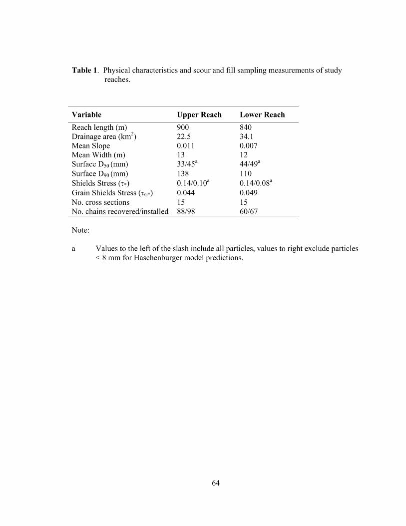
64

Table 1. Physical characteristics and scour and fill sampling measurements of study reaches.

Variable Upper Reach Lower Reach Reach length (m) 900 840 Drainage area (km2) 22.5 34.1 Mean Slope 0.011 0.007 Mean Width (m) 13 12 Surface D50 (mm) 33/45a 44/49a Surface D90 (mm) 138 110 Shields Stress (τ*) 0.14/0.10a 0.14/0.08a Grain Shields Stress (τG*) 0.044 0.049 No. cross sections 15 15 No. chains recovered/installed 88/98 60/67 Note: a Values to the left of the slash include all particles, values to right exclude particles

< 8 mm for Haschenburger model predictions.

65

Table 2. Summary of model constants, inputs, outputs (predictions), and measured values (for comparison).

Variables Units Upper Reach Lower Reach Model Constants Density of water: ρw kg/m3 1000 1000 Density of sediment: ρs kg/m3 2800a 2800 Reference shields stress: τr* --b 0.045c 0.045 Model Inputs Slope: S % 1.1 0.7 Median surface sediment size: D50 m 0.045 0.049 Hydraulic radius: R m 0.76 1.07 Model Outputs Shields Stress: τ* = (RSρw)/(ρs - ρw)D50 -- 0.10 0.08 Model parameter: θ = 3.33e-1.52τ*/τr* -- 0.102 0.189 Predicted mean scour/fill depth: 1/ θ cm 9.8 5.3 Measured Values Mean scour depth cm 10.6 6.0 Mean fill depth cm 10.2 13.3 Mean active layer depth cm 14.7 14.3 Note: a Typical value for metasedimentary and metamorphic rocks, which comprise the

majority of the that substrate in the upper and lower study reaches. b No units/dimensionless. c Reference shields stress value for incipient motion used by Haschenburger

(1999).

66

Table 3. Summary of statistical hypotheses testing results.

Null Hypothesis (and Statistical Test)

Parameter

n

Mean (cm)

σ

(cm)

Probability of Similarity

(P-value)a Redd construction does not redd scour 16 10.0 5.4 0.16 affect scour (paired t-test) control scour 16 7.8 6.1 difference 16 2.3 6.2 Scour is not a factor in redd reach scour 91 10.6 12.5 0.75 site selection (t-test) control scour 34 11.1 5.9 Redds are not prone to redd scour 16 10.0 5.4 0.04 aggradation (paired t-test) redd fill 16 16.0 8.0 difference 16 6.0 10.7 Redds are not prone to reach fill 93 10.2 8.3 0.12 aggradation (t-test) control fill 9 13.6 5.5

Note: a Paired and unpaired two-tailed t-tests were used assuming unequal and unknown

variances.

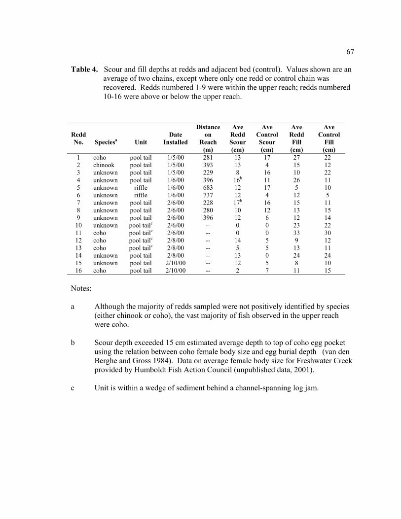
67

Table 4. Scour and fill depths at redds and adjacent bed (control). Values shown are an average of two chains, except where only one redd or control chain was recovered. Redds numbered 1-9 were within the upper reach; redds numbered 10-16 were above or below the upper reach.

Redd No.

Speciesa

Unit

Date

Installed

Distance on

Reach (m)

Ave Redd Scour (cm)

Ave Control Scour (cm)

Ave Redd Fill

(cm)

Ave Control

Fill (cm)

1 coho pool tail 1/5/00 281 13 17 27 22 2 chinook pool tail 1/5/00 393 13 4 15 12 3 unknown pool tail 1/5/00 229 8 16 10 22 4 unknown pool tail 1/6/00 396 16b 11 26 11 5 unknown riffle 1/6/00 683 12 17 5 10 6 unknown riffle 1/6/00 737 12 4 12 5 7 unknown pool tail 2/6/00 228 17b 16 15 11 8 unknown pool tail 2/6/00 280 10 12 13 15 9 unknown pool tail 2/6/00 396 12 6 12 14

10 unknown pool tailc 2/6/00 -- 0 0 23 22 11 coho pool tailc 2/6/00 -- 0 0 33 30 12 coho pool tailc 2/8/00 -- 14 5 9 12 13 coho pool tailc 2/8/00 -- 5 5 13 11 14 unknown pool tail 2/8/00 -- 13 0 24 24 15 unknown pool tail 2/10/00 -- 12 5 8 10 16 coho pool tail 2/10/00 -- 2 7 11 15

Notes: a Although the majority of redds sampled were not positively identified by species

(either chinook or coho), the vast majority of fish observed in the upper reach were coho.

b Scour depth exceeded 15 cm estimated average depth to top of coho egg pocket

using the relation between coho female body size and egg burial depth (van den Berghe and Gross 1984). Data on average female body size for Freshwater Creek provided by Humboldt Fish Action Council (unpublished data, 2001).

c Unit is within a wedge of sediment behind a channel-spanning log jam.

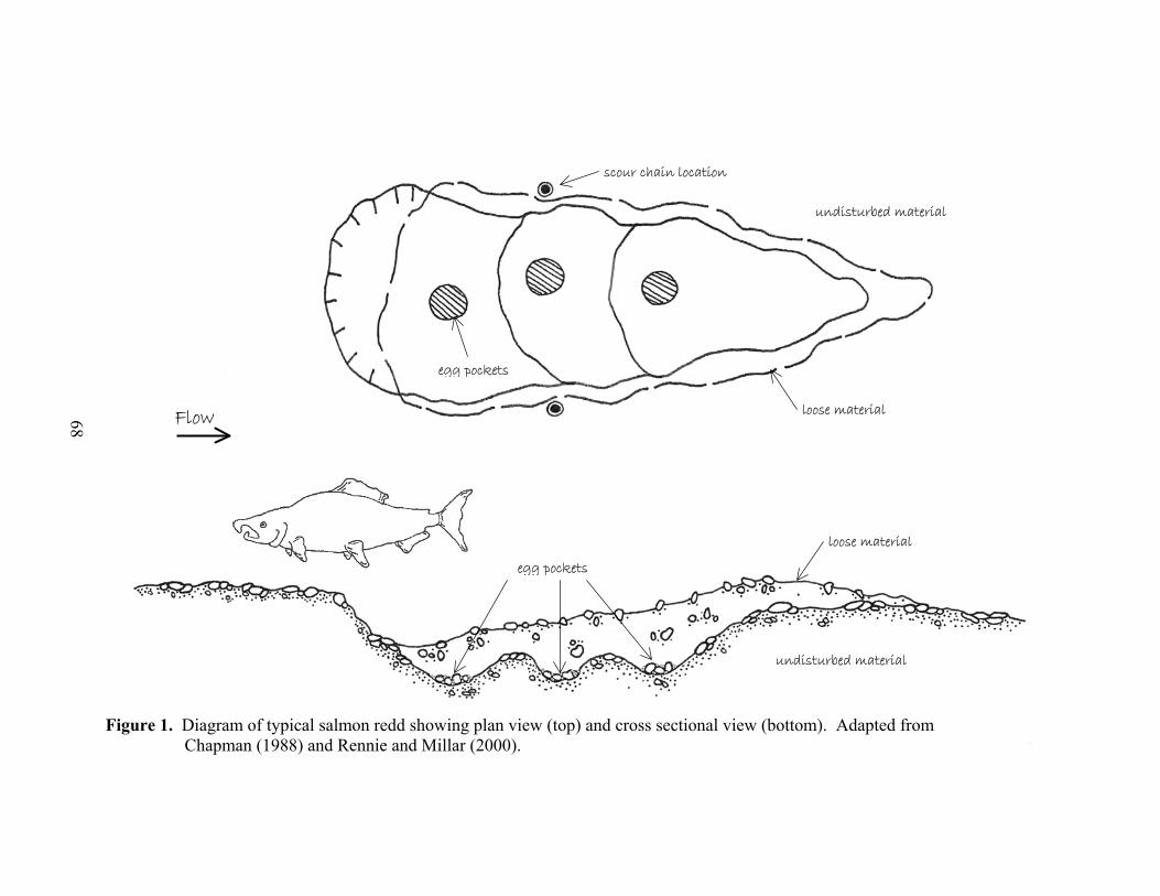
scour chain location

egg pockets

egg pockets

Flow 68

Figure 1. Diagram of typical salmon redd showing plan view (top) and cross sectional view

Chapman (1988) and Rennie and Millar (2000).

undisturbed material

loose material

undisturbed material

loose material

(bottom). Adapted from

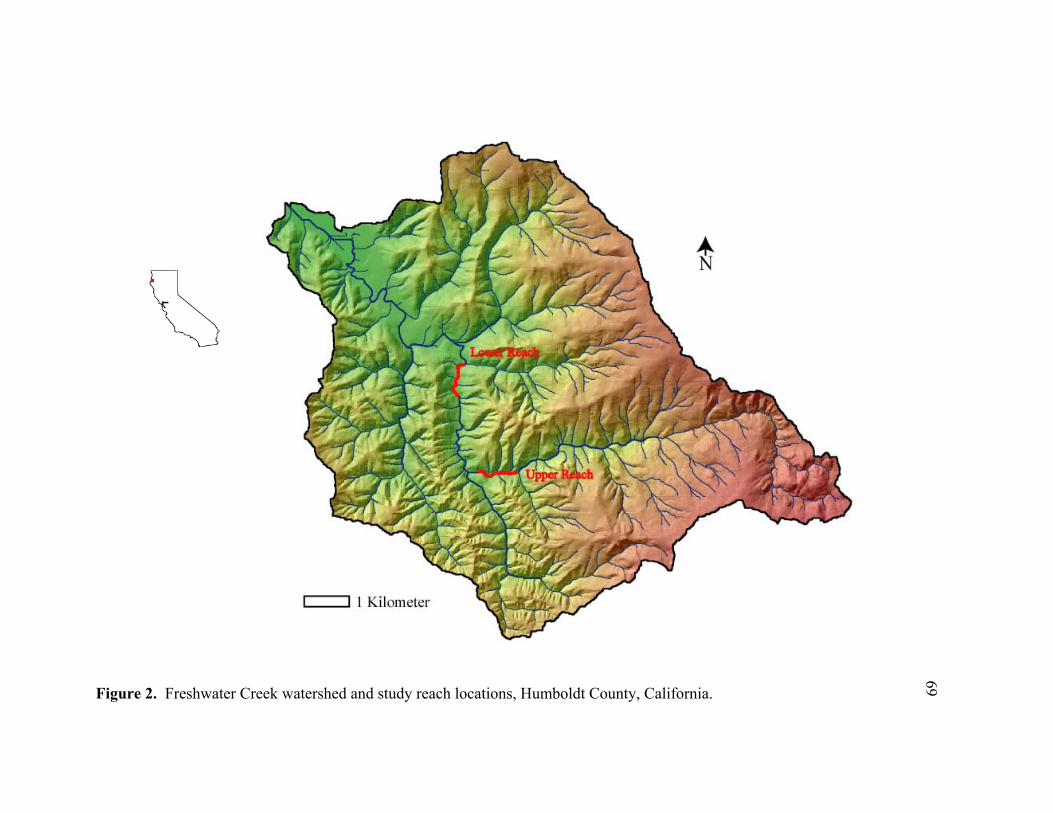
Figure 2. Freshwater Creek watershed and study reach locations, Humboldt County, California.

69

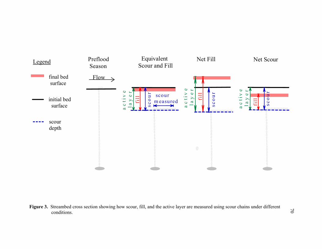
Equivalent Scour and Fill

Net Fill Net Scour

initial bed surface

final bed surface

scourdepth

Legend

ac

tiv

e l

ay

er

ac

tiv

e l

ay

er

ac

tiv

e l

ay

er

sco

ur

sco

ur

sco

ur

Preflood Season

scourm easured

Flow

fillfill fi

ll

Figure 3. Streambed cross section showing how scour, fill, and the active layer are measured using scour chains under different

conditions.

70

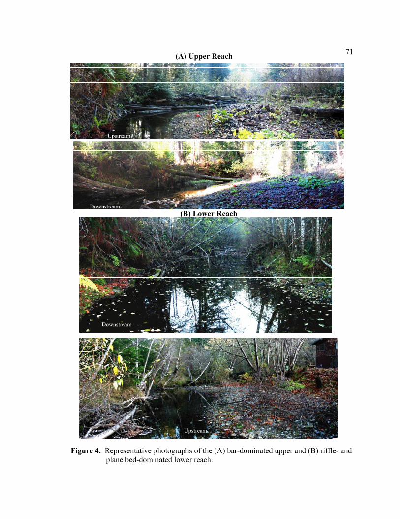
71

(A) Upper Reach Upstream

Downstream (B) Lower Reach

Downstream Upstream Figure 4. Representative photographs of the (A) bar-dominated upper and (B) riffle- and

plane bed-dominated lower reach.

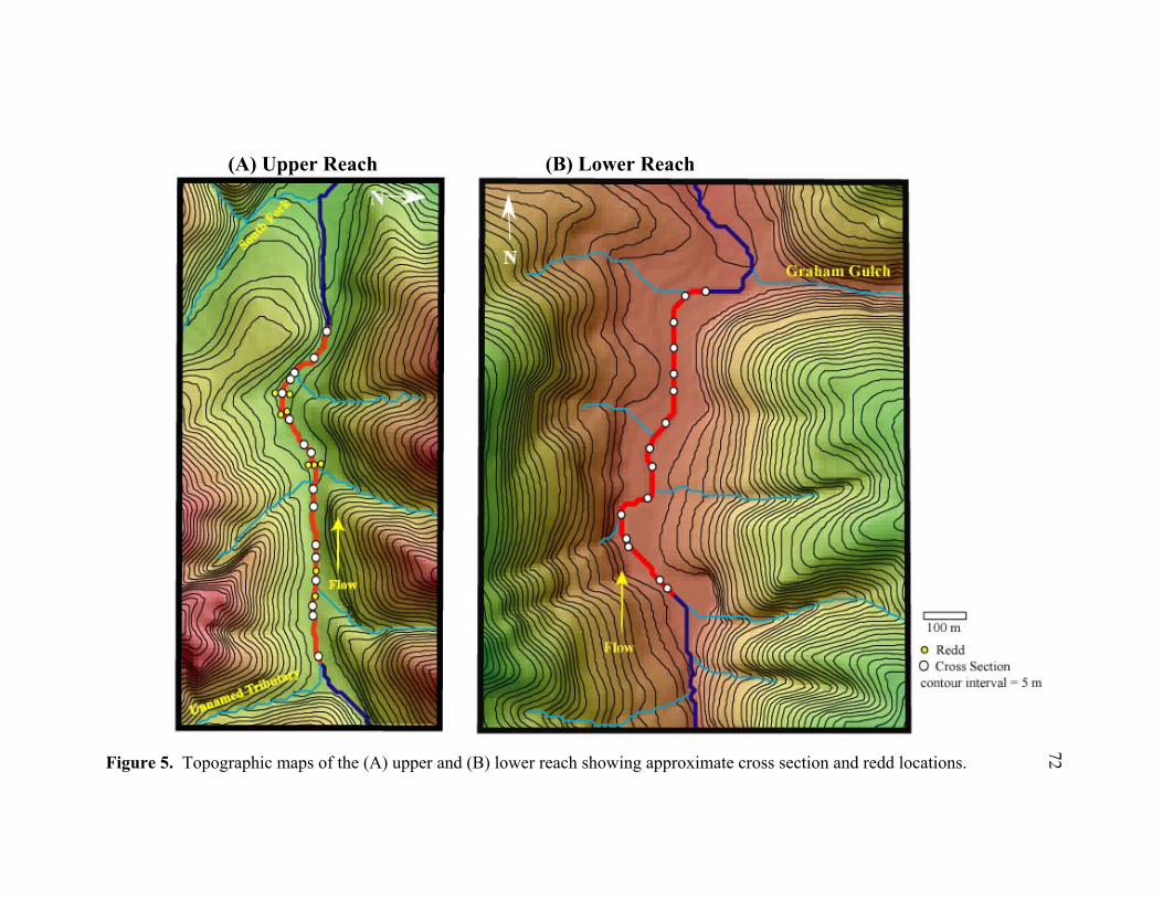
Figure 5. Topographic maps of the (A) upper and (B) lower reach showing approximate cross section and redd locations.

(A) Upper Reach (B) Lower Reach

72

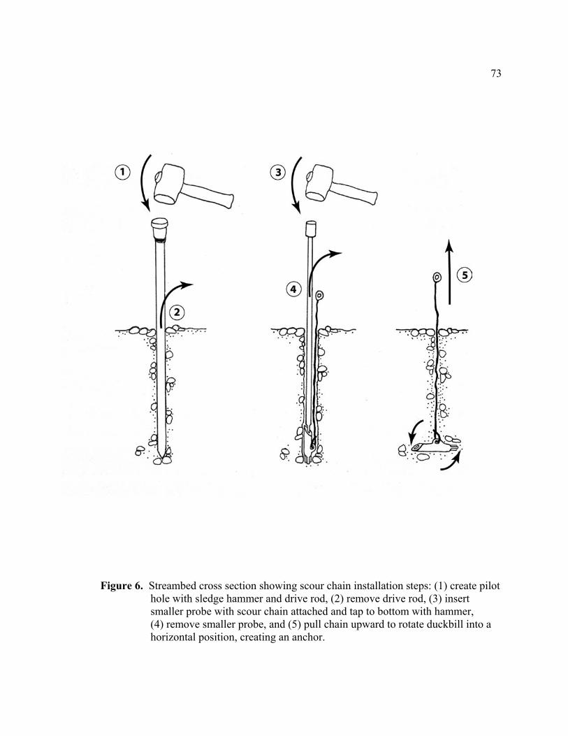
73

Figure 6. Streambed cross section showing scour chain installation steps: (1) create pilot

hole with sledge hammer and drive rod, (2) remove drive rod, (3) insert smaller probe with scour chain attached and tap to bottom with hammer, (4) remove smaller probe, and (5) pull chain upward to rotate duckbill into a horizontal position, creating an anchor.

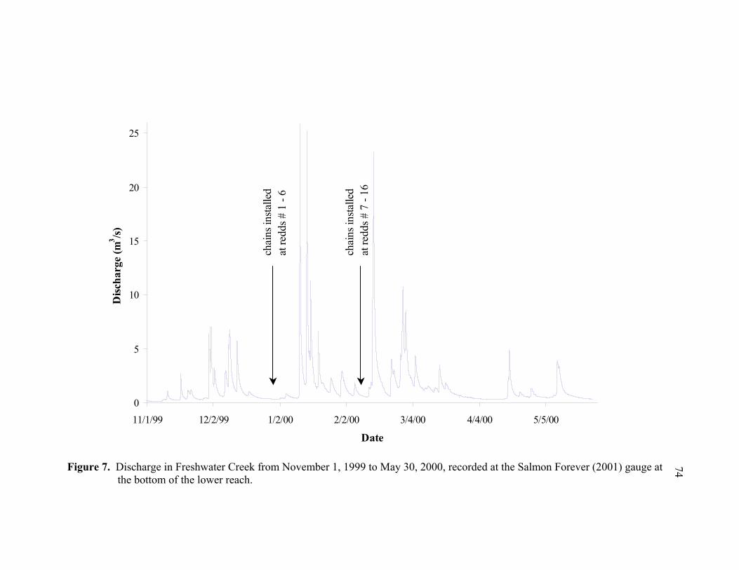
0

5

10

15

20

25

11/1/99 12/2/99 1/2/00 2/2/00 3/4/00 4/4/00 5/5/00

Date

Disc

harg

e (m

3 /s)

chai

ns in

stalle

d

at re

dds #

1 -

6d

chai

ns in

stalle

d

at re

dds #

7 -

16d

Figure 7. Discharge in Freshwater Creek from November 1, 1999 to May 30, 2000, recorded at the Salmon Forever (2001) gauge at the bottom of the lower reach.

74

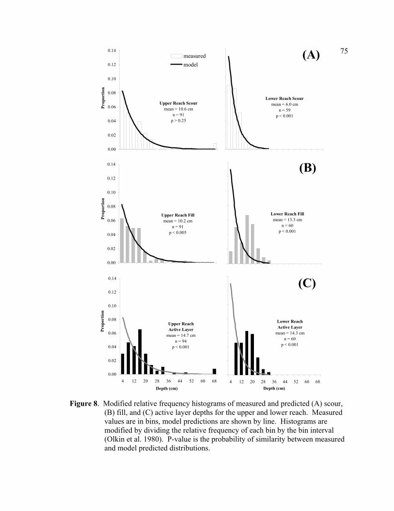
75

0.00

0.02

0.04

0.06

0.08

0.10

0.12

0.14

Prop

ortio

n

measuredmodel

Upper Reach Scourmean = 10.6 cm

n = 91p > 0.25

0.00

0.02

0.04

0.06

0.08

0.10

0.12

0.14

Prop

ortio

n

Upper Reach Fillmean = 10.2 cm

n = 91p < 0.005

0.00

0.02

0.04

0.06

0.08

0.10

0.12

0.14

4 12 20 28 36 44 52 60 68Depth (cm)

Prop

ortio

n

Upper Reach Active Layer

mean = 14.7 cmn = 94

p < 0.001

Lower Reach Scourmean = 6.0 cm

n = 59p < 0.001

(A)

Lower Reach Fillmean = 13.3 cm

n = 60p < 0.001

(B)

4 12 20 28 36 44 52 60 68Depth (cm)

Lower ReachActive Layer

mean = 14.3 cmn = 60

p < 0.001

(C)

Figure 8. Modified relative frequency histograms of measured and predicted (A) scour, (B) fill, and (C) active layer depths for the upper and lower reach. Measured values are in bins, model predictions are shown by line. Histograms are modified by dividing the relative frequency of each bin by the bin interval (Olkin et al. 1980). P-value is the probability of similarity between measured and model predicted distributions.

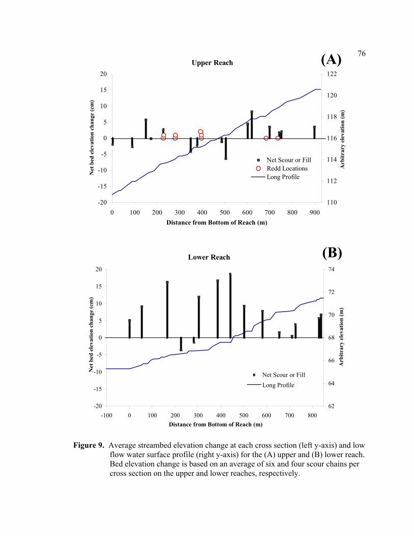
76

Upper Reach

-20

-15

-10

-5

0

5

10

15

20

0 100 200 300 400 500 600 700 800 900Distance from Bottom of Reach (m)

Net

bed

ele

vatio

n ch

ange

(cm

)

110

112

114

116

118

120

122

Arb

itrar

y el

evat

ion

(m)

Net Scour or FillRedd LocationsLong Profile

(A)

Lower Reach

-20

-15

-10

-5

0

5

10

15

20

-100 0 100 200 300 400 500 600 700 800Distance from Bottom of Reach (m)

Net

bed

ele

vatio

n ch

ange

(cm

)

62

64

66

68

70

72

74

Arb

itrar

y el

evat

ion

(m)

Net Scour or FillLong Profile

(B)

Figure 9. Average streambed elevation change at each cross section (left y-axis) and low flow water surface profile (right y-axis) for the (A) upper and (B) lower reach. Bed elevation change is based on an average of six and four scour chains per cross section on the upper and lower reaches, respectively.

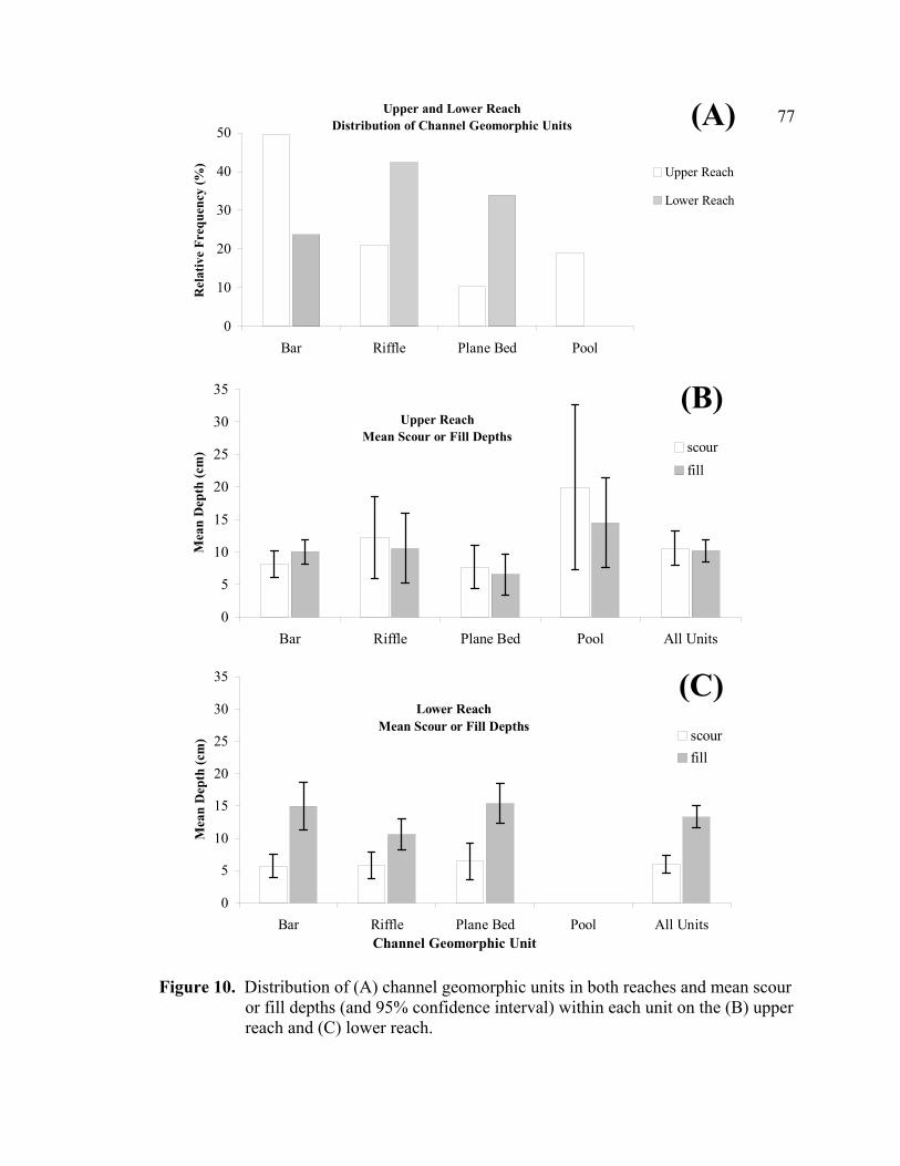
77

Upper and Lower Reach Distribution of Channel Geomorphic Units

0

10

20

30

40

50

Bar Riffle Plane Bed Pool

Rel

ativ

e Fr

eque

ncy

(%) Upper Reach

(A)

Upper ReachMean Scour or Fill Depths

0

5

10

15

20

25

30

35

Bar Riffle Plane Bed Pool All Units

Mea

n D

epth

(cm

) scourfill

(B)

Lower ReachMean Scour or Fill Depths

0

5

10

15

20

25

30

35

Bar Riffle Plane Bed Pool All UnitsChannel Geomorphic Unit

Mea

n D

epth

(cm

) scourfill

(C)

Lower Reach

Figure 10. Distribution of (A) channel geomorphic units in both reaches and mean scour or fill depths (and 95% confidence interval) within each unit on the (B) upper reach and (C) lower reach.

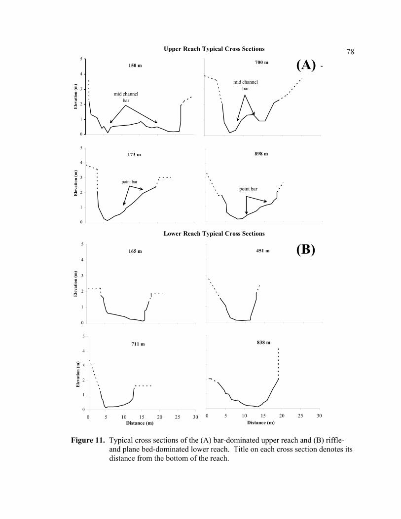
78

Upper Reach Typical Cross Sections

Lower Reach Typical Cross Sections

150 m

0

1

2

3

4

5

mid channel bar

700 m (A)mid channel

bar

173 m

0

1

2

3

4

5

point bar

898 m

point bar

165 m

0

1

2

3

4

5451 m (B)

711 m

0

1

2

3

4

5

0 5 10 15 20 25 30Distance (m)

Ele

vatio

n (m

)

838 m

0 5 10 15 20 25 30Distance (m)

Ele

vatio

n (m

)

Ele

vatio

n (m

)

Ele

vatio

n (m

)

Figure 11. Typical cross sections of the (A) bar-dominated upper reach and (B) riffle-

and plane bed-dominated lower reach. Title on each cross section denotes its distance from the bottom of the reach.

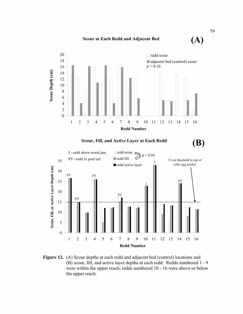
79

Scour at Each Redd and Adjacent Bed

02468

101214161820

1 2 3 4 5 6 7 8 9 10 11 12 13 14 15 16Redd Number

Scou

r D

epth

(cm

)redd scouradjacent bed (control) scour

(A)

p = 0.16

Scour, Fill, and Active Layer at Each Redd

0

5

10

15

20

25

30

35

1 2 3 4 5 6 7 8 9 10 11 12 13 14 15 16Redd Number

Scou

r, F

ill, o

r A

ctiv

e L

ayer

Dep

th (c

m)

redd scour

redd fill

redd active layer15 cm threshold to top of

coho egg pocket

(B) p = 0.04

J - redd above wood jam

J

PT PT

PT

PT

PT - redd in pool tail

J

PT

Figure 12. (A) Scour depths at each redd and adjacent bed (control) locations and (B) scour, fill, and active layer depths at each redd. Redds numbered 1 - 9 were within the upper reach; redds numbered 10 - 16 were above or below the upper reach.

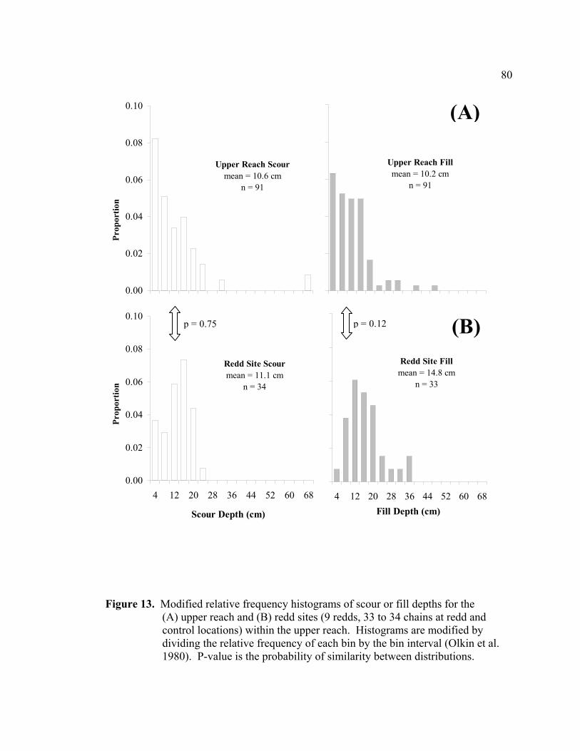
80

0.00

0.02

0.04

0.06

0.08

0.10Pr

opor

tion

Upper Reach Scourmean = 10.6 cm

n = 91

0.00

0.02

0.04

0.06

0.08

0.10

4 12 20 28 36 44 52 60 68

Scour Depth (cm)

Prop

ortio

n

Redd Site Scourmean = 11.1 cm

n = 34

p = 0.75

Upper Reach Fillmean = 10.2 cm

n = 91

(A)

4 12 20 28 36 44 52 60 68Fill Depth (cm)

Redd Site Fillmean = 14.8 cm

n = 33

(B)p = 0.12

Figure 13. Modified relative frequency histograms of scour or fill depths for the

(A) upper reach and (B) redd sites (9 redds, 33 to 34 chains at redd and control locations) within the upper reach. Histograms are modified by dividing the relative frequency of each bin by the bin interval (Olkin et al. 1980). P-value is the probability of similarity between distributions.

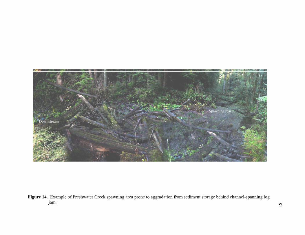
Downstream

Figure 14. Example of Freshwater Creek spawninjam.

g are

Spawning reach

a prone to aggradation from sediment storage behind channel-spanning log

81

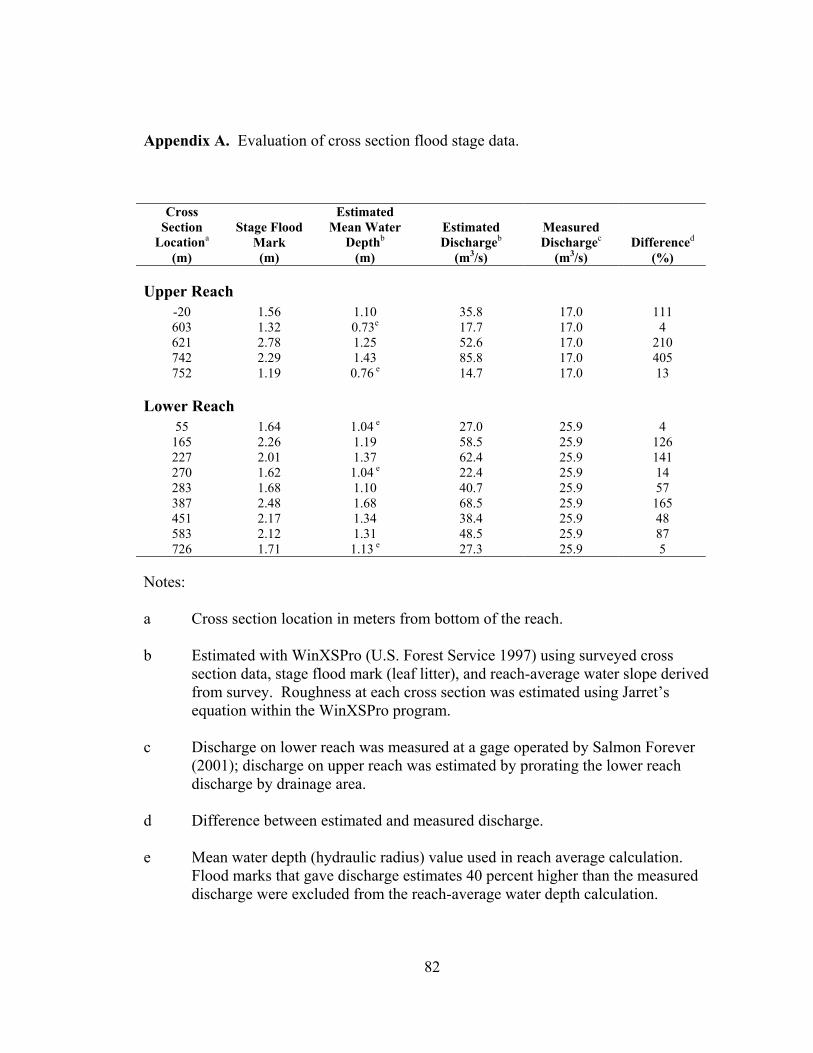
82

Appendix A. Evaluation of cross section flood stage data.

Cross Section

Locationa (m)

Stage Flood Mark (m)

Estimated Mean Water

Depthb (m)

Estimated Dischargeb

(m3/s)

Measured Dischargec

(m3/s) Differenced

(%)

Upper Reach -20 1.56 1.10 35.8 17.0 111 603 1.32 0.73e 17.7 17.0 4 621 2.78 1.25 52.6 17.0 210 742 2.29 1.43 85.8 17.0 405 752 1.19 0.76 e 14.7 17.0 13

Lower Reach 55 1.64 1.04 e 27.0 25.9 4

165 2.26 1.19 58.5 25.9 126 227 2.01 1.37 62.4 25.9 141 270 1.62 1.04 e 22.4 25.9 14 283 1.68 1.10 40.7 25.9 57 387 2.48 1.68 68.5 25.9 165 451 2.17 1.34 38.4 25.9 48 583 2.12 1.31 48.5 25.9 87 726 1.71 1.13 e 27.3 25.9 5

Notes: a Cross section location in meters from bottom of the reach. b Estimated with WinXSPro (U.S. Forest Service 1997) using surveyed cross

section data, stage flood mark (leaf litter), and reach-average water slope derived from survey. Roughness at each cross section was estimated using Jarret’s equation within the WinXSPro program.

c Discharge on lower reach was measured at a gage operated by Salmon Forever

(2001); discharge on upper reach was estimated by prorating the lower reach discharge by drainage area.

d Difference between estimated and measured discharge. e Mean water depth (hydraulic radius) value used in reach average calculation.

Flood marks that gave discharge estimates 40 percent higher than the measured discharge were excluded from the reach-average water depth calculation.

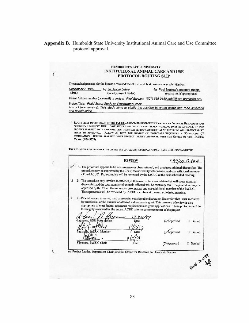
83

Appendix B. Humboldt State University Institutional Animal Care and Use Committee protocol approval.

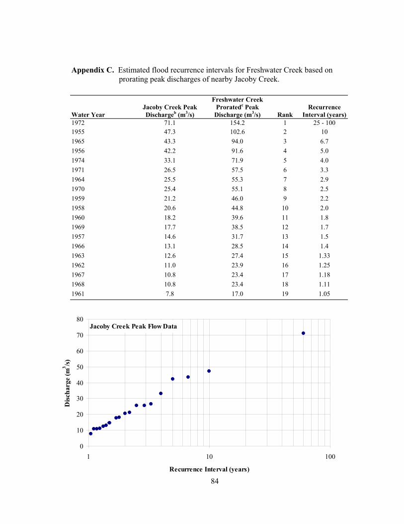
84

Appendix C. Estimated flood recurrence intervals for Freshwater Creek based on prorating peak discharges of nearby Jacoby Creek.

Water Year

Jacoby Creek Peak Dischargeb (m3/s)

Freshwater Creek Proratedc Peak

Discharge (m3/s)

Rank Recurrence

Interval (years)1972 71.1 154.2 1 25 - 100 1955 47.3 102.6 2 10 1965 43.3 94.0 3 6.7 1956 42.2 91.6 4 5.0 1974 33.1 71.9 5 4.0 1971 26.5 57.5 6 3.3 1964 25.5 55.3 7 2.9 1970 25.4 55.1 8 2.5 1959 21.2 46.0 9 2.2 1958 20.6 44.8 10 2.0 1960 18.2 39.6 11 1.8 1969 17.7 38.5 12 1.7 1957 14.6 31.7 13 1.5 1966 13.1 28.5 14 1.4 1963 12.6 27.4 15 1.33 1962 11.0 23.9 16 1.25 1967 10.8 23.4 17 1.18 1968 10.8 23.4 18 1.11 1961 7.8 17.0 19 1.05

Jacoby Creek Peak Flow Data

0

10

20

30

40

50

60

70

80

1 10 100

Recurrence Interval (years)

Disc

harg

e (m

3 /s)

85

Appendix C. (Continued) Estimated flood recurrence intervals for Freshwater Creek based on prorating peak discharges of nearby Jacoby Creek.

Date Freshwater Creek Peak

Discharged (m3/s) Estimated Recurrence Interval

(years)

January 11, 2000 25.9 1.3

January 14, 2000 25.2 1.3

February 14, 2000 23.2 1.1 Notes: a Jacoby Creek is a basin immediately north of Freshwater Creek. b source: U.S. Geological Survey, available at www.usgs.gov. c prorated by gage drainage area ratio (2.17) of Freshwater Creek (34.1 km2) to Jacoby Creek (15.7 km2). d source: Salmon Forever (2001).

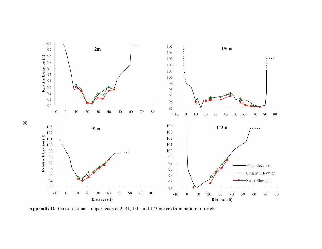
2m

90919293949596979899

100

-10 0 10 20 30 40 50 60 70 80

Rel

ativ

e E

leva

tion

(ft)

91m

93949596979899

100101102103

-10 0 10 20 30 40 50 60 70 80Distance (ft)

Rel

ativ

e E

leva

tion

(ft)

150m

9596979899

100101102103104105

-10 0 10 20 30 40 50 60 70 80 90

173m

949596979899

100101102103104

-10 0 10 20 30 40 50 60 70 80Distance (ft)

Final Elevation

Original Elevation

Scour Elevation

86

Appendix D. Cross sections – upper reach at 2, 91, 150, and 173 meters from bottom of reach.

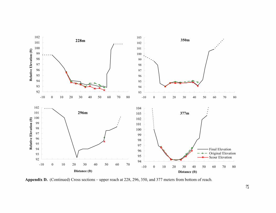
228m

9293949596979899

100101102

-10 0 10 20 30 40 50 60 70 80

Rel

ativ

e E

leva

tion

(ft)

296m

9293949596979899

100101102

-10 0 10 20 30 40 50 60 70

Distance (ft)

Rel

ativ

e E

leva

tion

(ft)

350m

93

94

95

96

97

98

99

100

101

102

103

-10 0 10 20 30 40 50 60 70 80

377m

949596979899

100101102103104

-10 0 10 20 30 40 50 60 70 80Distance (ft)

Final ElevationOriginal ElevationScour Elevation

Appendix D. (Continued) Cross sections – upper reach at 228, 296, 350, and 377 meters from bottom of reach.

87

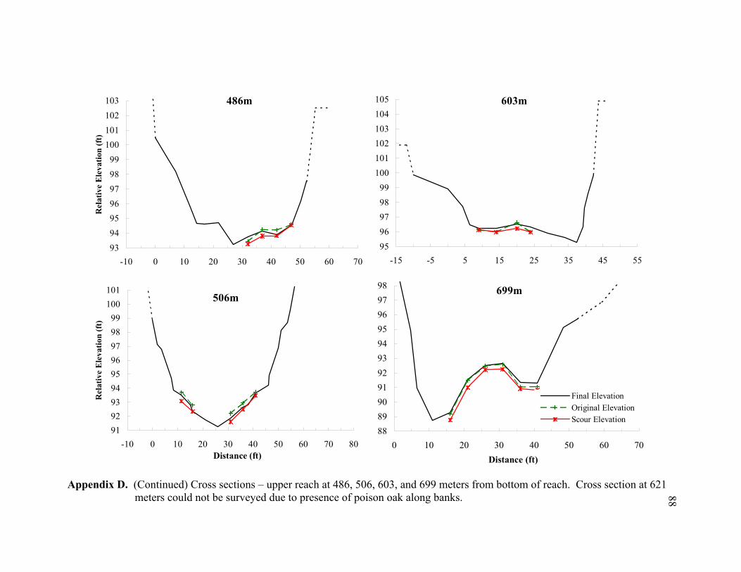
486m

93949596979899

100101102103

-10 0 10 20 30 40 50 60 70

Rel

ativ

e E

leva

tion

(ft)

506m

919293949596979899

100101

-10 0 10 20 30 40 50 60 70 80Distance (ft)

Rel

ativ

e E

leva

tion

(ft)

603m

9596979899

100101102103104105

-15 -5 5 15 25 35 45 55

699m

8889909192939495969798

0 10 20 30 40 50 60 70Distance (ft)

Final ElevationOriginal ElevationScour Elevation

Appendix D. (Continued) Cross sections – upper reach at 486, 506, 603, and 699 meters from bottom of reach. Cross section at 621

meters could not be surveyed due to presence of poison oak along banks. 88

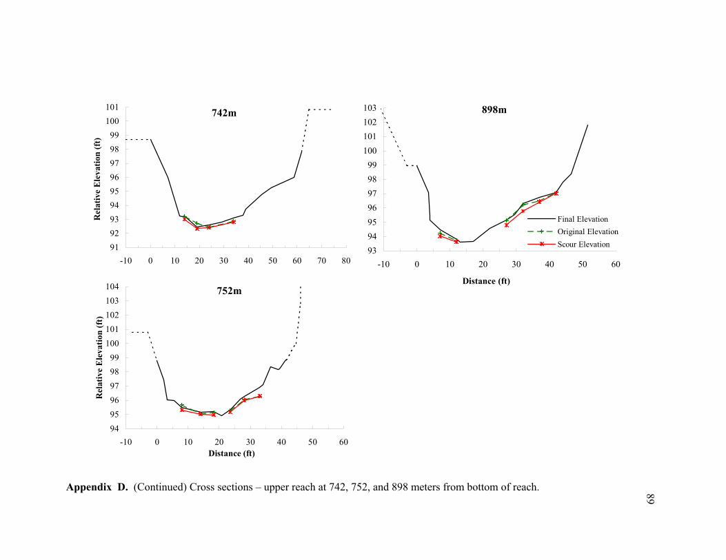
742m

919293949596979899

100101

-10 0 10 20 30 40 50 60 70 80

Rel

ativ

e E

leva

tion

(ft)

752m

949596979899

100101102103104

-10 0 10 20 30 40 50 60Distance (ft)

Rel

ativ

e E

leva

tion

(ft)

898m

93949596979899

100101102103

-10 0 10 20 30 40 50 60

Distance (ft)

Final ElevationOriginal ElevationScour Elevation

Appendix D. (Continued) Cross sections – upper reach at 742, 752, and 898 meters from bottom of reach. 89

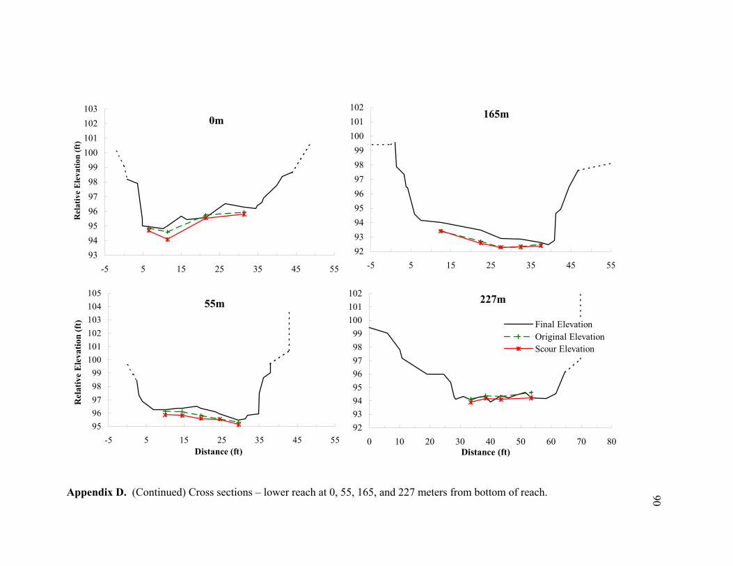
55m

9596979899

100101102103104105

-5 5 15 25 35 45 55Distance (ft)

Rel

ativ

e E

leva

tion

(ft)

165m

9293949596979899

100101102

-5 5 15 25 35 45 55

227m

9293949596979899

100101102

0 10 20 30 40 50 60 70 80Distance (ft)

Final ElevationOriginal ElevationScour Elevation

0m

93949596979899

100101102103

-5 5 15 25 35 45 55

Rel

ativ

e E

leva

tion

(ft)

Appendix D. (Continued) Cross sections – lower reach at 0, 55, 165, and 227 meters from bottom of reach. 90

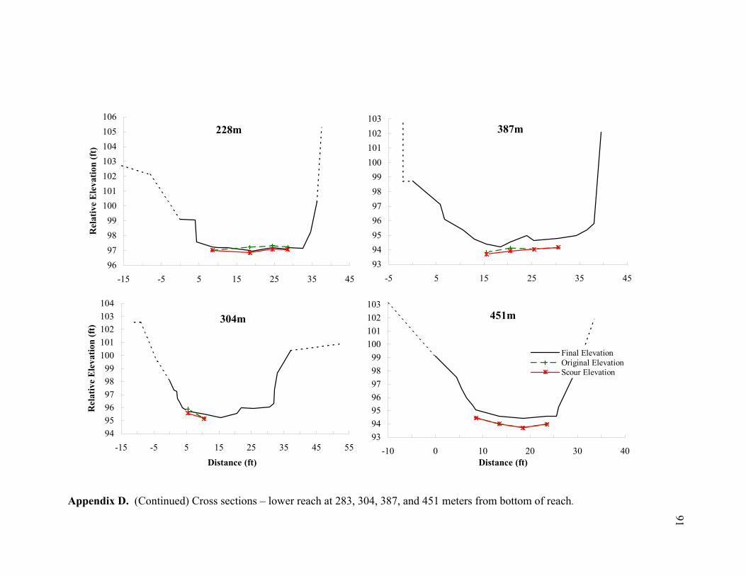
304m

949596979899

100101102103104

-15 -5 5 15 25 35 45 55Distance (ft)

Rel

ativ

e E

leva

tion

(ft)

228m

96979899

100101102103104105106

-15 -5 5 15 25 35 45

Rel

ativ

e E

leva

tion

(ft)

387m

93949596979899

100101102103

-5 5 15 25 35 45

451m

93949596979899

100101102103

-10 0 10 20 30 40Distance (ft)

Final ElevationOriginal ElevationScour Elevation

Appendix D. (Continued) Cross sections – lower reach at 283, 304, 387, and 451 meters from bottom of reach.

91

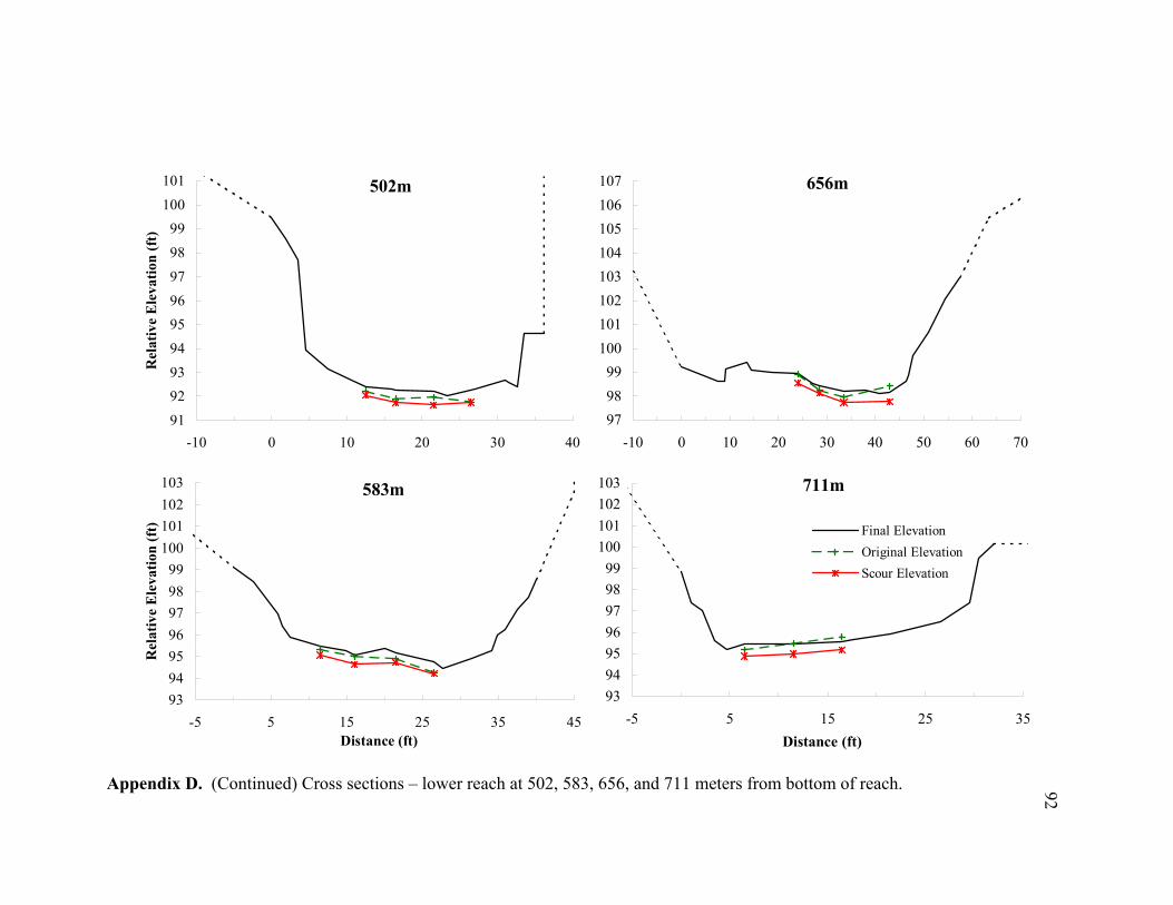
502m

919293949596979899

100101

-10 0 10 20 30 40

Rel

ativ

e E

leva

tion

(ft)

583m

93949596979899

100101102103

-5 5 15 25 35 45Distance (ft)

Rel

ativ

e E

leva

tion

(ft)

656m

979899

100101102103104105106107

-10 0 10 20 30 40 50 60 70

711m

93949596979899

100101102103

-5 5 15 25 35Distance (ft)

Final ElevationOriginal ElevationScour Elevation

Appendix D. (Continued) Cross sections – lower reach at 502, 583, 656, and 711 meters from bottom of reach. 92

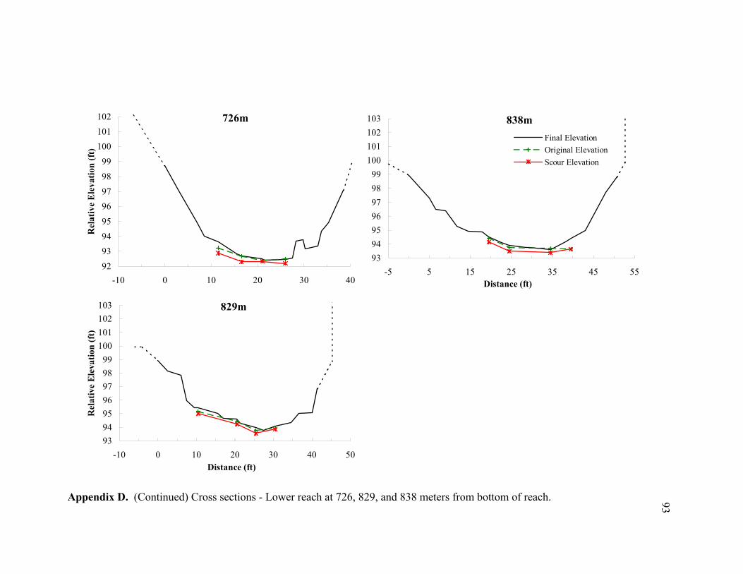
726m

9293949596979899

100101102

-10 0 10 20 30 40

Rel

ativ

e E

leva

tion

(ft)

829m

93949596979899

100101102103

-10 0 10 20 30 40 50Distance (ft)

Rel

ativ

e E

leva

tion

(ft)

838m

93949596979899

100101102103

-5 5 15 25 35 45 55Distance (ft)

Final ElevationOriginal ElevationScour Elevation

Appendix D. (Continued) Cross sections - Lower reach at 726, 829, and 838 meters from bottom of reach. 93

94

Appendix E. Scour and fill measurements – upper reach.

XS Location

(m) a

Station

(m)

Channel Geomorph

Unit

Scour (cm)

Fill (cm)

Active Layer (cm)

Net Change

(cm)

XS Net Change

(cm) Notes

2 2.9 bar 13.3 5.1 13.3 -8.3 -2.0 4.4 bar 7.6 0.0 7.6 -7.6 5.9 plane bed 5.1 2.5 5.1 -2.5 7.5 plane bed 7.6 2.5 7.6 -5.1 9.0 bar 23.5 12.7 23.5 -10.8 10.5 bar 16.5 38.1 38.1 21.6 12.0 bar 21.0 17.8 21.0 -3.2 13.6 bar 0.0 0.0 0.0 0.0

91 3.4 plane bed 11.4 5.7 11.4 -5.7 -2.7 4.6 plane bed 14.0 9.5 14.0 -4.4 6.4 plane bed 22.2 6.4 22.2 -15.9 7.9 plane bed 10.8 8.9 10.8 -1.9 9.4 bar 3.2 7.6 7.6 4.4 11.0 bar 4.4 7.6 7.6 3.2 12.2 bar 1.3 2.5 2.5 1.3

150 3.0 bar 3.2 5.1 5.1 1.9 5.7 6.1 bar 0.0 12.7 12.7 12.7 7.6 bar 14.0 8.9 14.0 -5.1 10.7 bar 11.4 14.0 14.0 2.5 13.7 bar 9.5 16.5 16.5 7.0 16.8 bar 19.1 7.6 19.1 -11.4 18.3 pool 0.0 27.3 27.3 27.3 20.1 pool 5.7 16.5 16.5 10.8 22.9 cohesive bed, no chain

173 1.8 pool 7.0 15.2 15.2 8.3 -0.1 3.4 pool 30.5 over 1' of fill, no chain recovery 4.9 pool 30.5 over 1' of fill, no chain recovery 6.4 bar 29.2 17.8 29.2 -11.4 7.9 bar 6.4 11.4 11.4 5.1 9.4 bar 17.1 15.2 17.1 -1.9 11.0 bar 8.3 7.6 8.3 -0.6

228 4.6 bar 3.8 0.0 3.8 -3.8 2.7 6.1 bar 5.7 10.2 10.2 4.4 7.6 bar 1.3 12.7 12.7 11.4 9.1 bar 4.4 15.2 15.2 10.8 10.7 bar 3.2 15.2 15.2 12.1 12.2 riffle 17.1 10.2 17.1 -7.0 13.7 riffle 30.5 22.9 30.5 -7.6 15.2 riffle 17.1 15.9 17.1 -1.3 16.8 riffle 14.0 19.1 19.1 5.1

296 8.5 pool 64.1 chain scoured out completely 10.1 pool 66.7 chain scoured out completely 11.6 pool 66.7 chain scoured out completely 13.1 pool 45.7 over 1.5' of fill, no chain recovery 14.6 pool 22.9 3.8 22.9 -19.1

350 3.4 plane bed 0.0 1.3 1.3 1.3 -4.1 4.9 plane bed 0.0 0.0 0.0 0.0 6.4 plane bed 7.0 7.6 7.6 0.6 7.9 plane bed 5.1 2.5 5.1 -2.5 9.8 bedrock, no chain installation 11.7 plane bed 8.3 2.5 8.3 -5.7 13.3 plane bed 21.0 2.5 21.0 -18.4

95

Appendix E. (Continued) Scour and fill measurements – upper reach.

XS Location

(m)

Station

(m)

Channel Geomorph

Unit

Scour (cm)

Fill (cm)

Active Layer (cm)

Net Change

(cm)

XS Net Change

(cm) Notes

377 2.1 bar 5.1 0.0 5.1 -5.1 -2.3 3.7 1' to clay bed, no chain 5.2 pool 0.0 3.8 3.8 3.8 6.7 water too deep for chain recovery 8.2 pool 1.3 5.1 5.1 3.8 9.8 pool 12.1 5.1 12.1 -7.0 11.6 pool 17.1 10.2 17.1 -7.0

486 2.1 -1.1 bedrock/boulders, no chain 3.7 bedrock/boulders, no chain 5.2 bedrock/boulders, no chain 6.7 bedrock/boulders, no chain 8.2 bedrock/boulders, no chain 9.8 riffle 5.1 15.2 15.2 10.2 11.3 riffle 13.3 9.5 13.3 -3.8 12.8 riffle 12.1 2.5 12.1 -9.5 14.3 riffle 1.3 0.0 1.3 -1.3

506 3.5 pool 19.1 0.0 19.1 -19.1 -6.4 4.9 pool 13.3 2.5 13.3 -10.8 6.4 1' to bedrock, no chain 7.9 bedrock, no chain installation 9.4 bar 18.4 10.2 18.4 -8.3 11.0 bar 13.3 12.7 13.3 -0.6 12.5 bar 8.3 15.2 15.2 7.0

603 2.7 bar 0.0 3.8 3.8 3.8 4.4 4.3 bar 0.0 7.6 7.6 7.6 6.1 bar 12.7 8.9 12.7 -3.8 7.3 bar 0.0 10.2 10.2 10.2 8.8 1' to bedrock, no chain 10.4 1' to bedrock, no chain

621 2.1 bar 14.6 10.2 14.6 -4.4 8.3 3.7 bar 5.1 5.7 5.7 0.6 5.2 plane bed 2.5 25.4 25.4 22.9 6.7 plane bed 3.8 17.8 17.8 14.0 8.2 water too deep for chain recovery 9.8 cohesive bed, no chain 11.3 cohesive bed, no chain

699 3.4 pool 3.5 wood, chain installation not possible 4.9 pool 13.3 15.2 15.2 1.9 6.4 bar 14.6 15.9 15.9 1.3 7.9 bar 8.3 8.9 8.9 0.6 9.4 bar 10.2 11.4 11.4 1.3 11.0 bar 3.8 12.7 12.7 8.9 12.5 bar 7.0 14.0 14.0 7.0

742 4.3 bar 6.4 7.6 7.6 1.3 1.7 5.8 riffle 11.4 3.8 11.4 -7.6 7.3 riffle 0.0 6.4 6.4 6.4 8.8 boulders, no chain installation 10.4 bar 1.9 8.9 8.9 7.0 11.9 boulders, no chain installation 12.5 boulders, no chain installation

96

Appendix E. (Continued) Scour and fill measurements – upper reach.

XS Location

(m)

Station

(m)

Channel Geomorph

Unit

Scour (cm)

Fill (cm)

Active Layer (cm)

Net Change

(cm)

XS Net Change

(cm) Notes

752 2.4 plane bed 10.8 6.4 10.8 -4.4 2.0 4.3 plane bed 0.0 3.8 3.8 3.8 5.6 plane bed 5.1 7.6 7.6 2.5 7.2 plane bed 2.5 5.1 5.1 2.5 8.5 bar 1.3 8.9 8.9 7.6 10.1 bar 0.0 0.0 0.0 0.0

898 2.1 pool 6.4 14.0 14.0 7.6 3.5 3.7 pool 3.2 5.7 5.7 2.5 5.2 boulders, no chain installation 6.7 water too deep for chain recovery 8.2 bar 9.5 10.2 10.2 0.6 9.8 bar 13.3 15.9 15.9 2.5 11.3 bar 1.9 9.5 9.5 7.6 12.8 bar 1.3 1.3 1.3 0.0

Reach Average:

10.6

10.2

12.2

0.6

0.9

Note: a Cross section (XS) location is the distance in meters from the bottom of the reach.

97

Appendix E. (Continued) Scour and fill measurements – lower reach.

XS Locationa

(m)

Station

(m)

Channel Geomorph

Unit

Scour (cm)

Fill (cm)

Active Layer (cm)

Net Change

(cm)

XS Net Change

(cm) Notes

0 2.0 plane bed 5.7 7.6 7.6 1.9 5.1 3.5 plane bed 15.2 27.9 27.9 12.7 5.0 bar over 1’ fill, no chain recovery 6.6 bar 6.4 1.3 6.4 -5.1 8.1 alder, no chain installation 9.6 bar 3.8 14.6 14.6 10.8

55 3.0 bar 7.6 11.4 11.4 3.8 9.1 4.4 bar 8.3 16.5 16.5 8.3 5.9 bar 6.4 22.9 22.9 16.5 7.5 riffle 0.0 12.7 12.7 12.7 9.0 riffle 5.7 10.2 10.2 4.4

165 2.3 16.3 cohesive bed, no chain installation 3.8 bar 0.0 17.8 17.8 17.8 5.3 wood, no chain installation 6.9 bar 3.8 27.9 27.9 24.1 8.4 riffle 0.0 19.1 19.1 19.1 9.9 riffle 0.0 16.5 16.5 16.5 11.4 riffle 3.8 7.6 7.6 3.8

227 7.2 bar -3.7 couldn't discern bend in chain 8.7 riffle wood, no chain installation 10.2 riffle 7.0 5.1 7.0 -1.9 11.7 riffle 6.4 4.4 6.4 -1.9 13.3 riffle 6.4 7.6 7.6 1.3 14.8 boulders, no chain installation 16.3 riffle 12.1 0.0 12.1 -12.1 17.8 cohesive bed, no chain installation

283 2.6 riffle 0.0 6.4 6.4 6.4 -1.4 4.1 bedrock, no chain installation 5.6 riffle 11.4 3.8 11.4 -7.6 7.5 riffle 7.0 3.8 7.0 -3.2 8.7 riffle 5.7 4.4 5.7 -1.3 10.2

304 1.7 plane bed 10.2 5.1 10.2 -5.1 11.9 3.2 plane bed 0.0 10.2 10.2 10.2 4.7 plane bed 30.5 30.5 30.5 over 1’ fill, no chain recovery 6.2 wood, no chain installation 7.8 plane bed no magnet, could not relocate chain 9.3 bedrock, no chain installation

387 3.2 16.7 bedrock, no chain installation 4.7 riffle 3.8 21.6 21.6 17.8 6.2 riffle 6.4 19.1 19.1 12.7 7.8 riffle 0.0 17.8 17.8 17.8 9.3 riffle 0.0 18.4 18.4 18.4 10.8 bedrock, no chain installation

451 2.6 plane bed 0.0 17.8 17.8 17.8 18.6 4.1 plane bed 0.0 17.1 17.1 17.1 5.6 plane bed 0.0 21.6 21.6 21.6 7.2 plane bed 0.0 17.8 17.8 17.8

502 3.8 plane bed 5.1 10.2 10.2 5.1 9.2 5.0 plane bed 5.1 15.2 15.2 10.2 6.6 plane bed 10.2 17.1 17.1 7.0 8.1 plane bed 0.6 15.2 15.2 14.6 9.6 cohesive bed, no chain installation

98

Appendix E. (Continued) Scour and fill measurements – lower reach.

XS Locationa

(m)

Station

(m)

Channel Geomorph

Unit

Scour (cm)

Fill (cm)

Active Layer (cm)

Net Change

(cm)

XS Net Change

(cm) Notes

583 3.5 bar 7.6 12.1 12.1 4.4 7.8 4.9 bar 10.8 12.7 12.7 1.9 6.6 bar 5.7 14.0 14.0 8.3 8.1 plane bed 1.3 17.8 17.8 16.5 9.6 cohesive bed, no chain installation

656 7.3 riffle 12.1 12.7 12.7 0.6 1.4 8.7 riffle 4.4 10.2 10.2 5.7 10.2 riffle 6.4 14.0 14.0 7.6 11.6 bedrock, no chain installation 13.1 riffle 20.3 12.1 20.3 -8.3

711 2.0 plane bed 9.5 17.1 17.1 7.6 0.4 3.5 plane bed 15.2 15.2 15.2 0.0 5.0 plane bed 18.4 12.1 18.4 -6.4 6.6 bedrock, no chain installation 8.1 chain broke upon recovery

726 3.5 plane bed 10.2 22.9 22.9 12.7 3.8 5.0 plane bed 11.4 12.1 12.1 0.6 6.4 plane bed 1.9 5.1 5.1 3.2 7.9 plane bed 8.9 7.6 8.9 -1.3 9.6 wood, no chain installation

829 3.2 bar 4.4 12.7 12.7 8.3 5.7 4.7 chain broke upon retrieval 6.2 bar 6.4 11.4 11.4 5.1 7.8 riffle 6.4 12.7 12.7 6.4 9.3 riffle 3.2 6.4 6.4 3.2 10.8 bedrock, no chain installation

838 4.4 6.7 no magnet, could not relocate chain 5.9 bar 8.9 11.4 11.4 2.5 7.5 riffle 8.3 12.7 12.7 4.4 9.0 no magnet, could not relocate chain 10.5 riffle 9.5 6.4 9.5 -3.2 12.0 bar 0.0 22.9 22.9 22.9

Reach Average:

6.0

13.3

14.3

7.4

7.2

Note: a Cross section (XS) location is the distance in meters from the bottom of the reach.

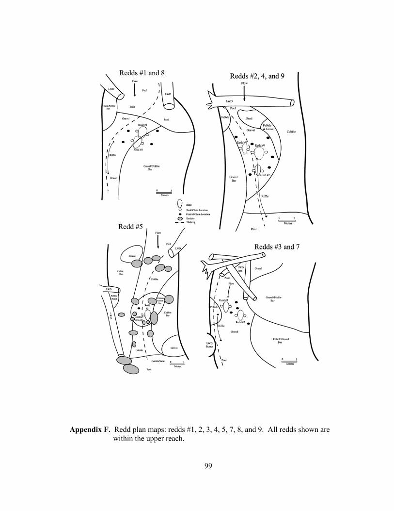
Appendix F. Redd plan maps: redds #1, 2, 3, 4, 5, 7, 8, and 9. All redds shown are

within the upper reach.

99

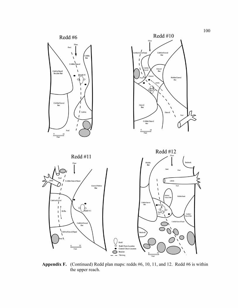
100

Appendix F. (Continued) Redd plan maps: redds #6, 10, 11, and 12. Redd #6 is within

the upper reach.

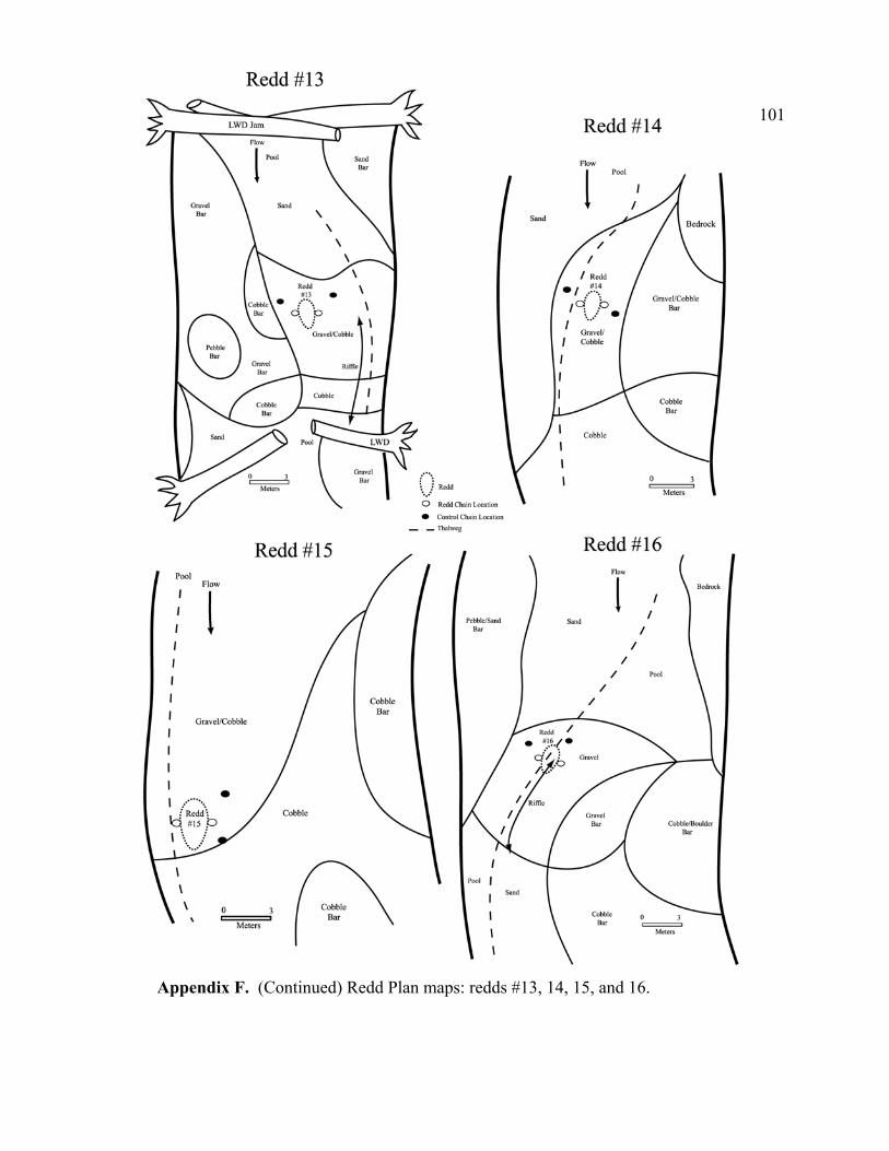
101

Appendix F. (Continued) Redd Plan maps: redds #13, 14, 15, and 16.

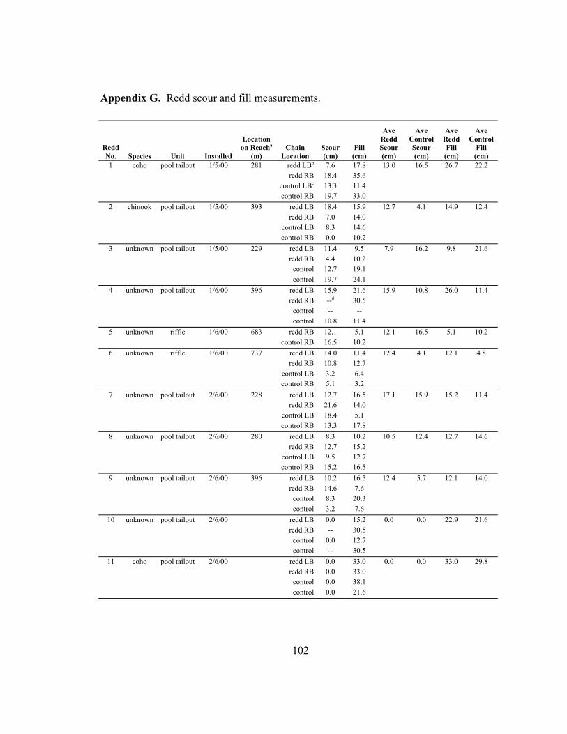
Appendix G. Redd scour and fill measurements.

Redd No.

Species

Unit

Installed

Location on Reacha

(m)

Chain Location

Scour (cm)

Fill (cm)

Ave Redd Scour (cm)

Ave Control Scour (cm)

Ave Redd Fill (cm)

Ave Control

Fill (cm)

1 coho pool tailout 1/5/00 281 redd LBb 7.6 17.8 13.0 16.5 26.7 22.2 redd RB 18.4 35.6 control LBc 13.3 11.4 control RB 19.7 33.0

2 chinook pool tailout 1/5/00 393 redd LB 18.4 15.9 12.7 4.1 14.9 12.4 redd RB 7.0 14.0 control LB 8.3 14.6 control RB 0.0 10.2

3 unknown pool tailout 1/5/00 229 redd LB 11.4 9.5 7.9 16.2 9.8 21.6 redd RB 4.4 10.2 control 12.7 19.1 control 19.7 24.1

4 unknown pool tailout 1/6/00 396 redd LB 15.9 21.6 15.9 10.8 26.0 11.4 redd RB --d 30.5 control -- -- control 10.8 11.4

5 unknown riffle 1/6/00 683 redd RB 12.1 5.1 12.1 16.5 5.1 10.2 control RB 16.5 10.2

6 unknown riffle 1/6/00 737 redd LB 14.0 11.4 12.4 4.1 12.1 4.8 redd RB 10.8 12.7 control LB 3.2 6.4 control RB 5.1 3.2

7 unknown pool tailout 2/6/00 228 redd LB 12.7 16.5 17.1 15.9 15.2 11.4 redd RB 21.6 14.0 control LB 18.4 5.1 control RB 13.3 17.8

8 unknown pool tailout 2/6/00 280 redd LB 8.3 10.2 10.5 12.4 12.7 14.6 redd RB 12.7 15.2 control LB 9.5 12.7 control RB 15.2 16.5

9 unknown pool tailout 2/6/00 396 redd LB 10.2 16.5 12.4 5.7 12.1 14.0 redd RB 14.6 7.6 control 8.3 20.3 control 3.2 7.6

10 unknown pool tailout 2/6/00 redd LB 0.0 15.2 0.0 0.0 22.9 21.6 redd RB -- 30.5 control 0.0 12.7 control -- 30.5

11 coho pool tailout 2/6/00 redd LB 0.0 33.0 0.0 0.0 33.0 29.8 redd RB 0.0 33.0 control 0.0 38.1 control 0.0 21.6

102

103

Appendix G. (Continued) Redd scour and fill measurements.

Redd No.

Species

Unit

Installed

Location on Reacha

(m)

Chain Location

Scour (cm)

Fill (cm)

Ave Redd Scour (cm)

Ave Control Scour (cm)

Ave Redd Fill (cm)

Ave Control

Fill (cm)

12 coho pool tailout 2/8/00 redd LB 13.3 12.1 14.0 5.1 9.2 12.4 redd RB 14.6 6.4 control 8.3 14.6 control 1.9 10.2

13 coho pool tailout 2/8/00 redd LB 1.9 10.2 5.1 4.8 13.3 11.4 redd RB 8.3 16.5 control 4.4 10.2 control 5.1 12.7

14 unknown pool tailout 2/8/00 redd LB 13.3 17.8 13.3 0.0 24.1 24.1 redd RB -- 30.5 control 0.0 17.8 control -- 30.5

15 unknown pool tailout 2/10/00 redd LB 14.0 6.4 12.4 5.1 8.3 10.2 redd RB 10.8 10.2 control 1.3 8.9 control 8.9 11.4

16 coho pool tailout 2/10/00 redd LB 3.8 12.7 1.9 7.3 11.4 14.6 redd RB 0.0 10.2 control 10.8 15.2 control 3.8 14.0

Notes: a Location for redds # 1 - 9 is distance from bottom of the upper reach, redds # 10 - 16 were above or below the upper reach. b Left bank facing downstream. c Right bank facing downstream. d No chain recovery