Embed Size (px)
Citation preview
April 2013
North Coast Regional Water Board, SWRCB Contract 09-084-110 and 11-189-110.
Scott Valley Integrated Hydrologic Model:
Data Collection, Analysis, and Water Budget
Final Report
Prepared by:
Laura Foglia, Alison McNally, Courtney Hall, Lauren Ledesma, Ryan Hines, and Thomas Harter
Department of Land, Air, and Water Resources
University of California, Davis
UC Davis 2 Final Report, April 22, 2013
Prepared for:
North Coast Regional Water Board
With funding by:
North Coast Regional Water Board, Contract #09-084-110
State Water Resources Control Board, Contract #11-189-110
FINAL REPORT
Version
April 22, 2013
©2013 The Regents of the University of California University of California – Davis
All rights reserved.

UC Davis 3 Final Report, April 22, 2013
Suggested Citation:
Foglia, L., A. McNally, C. Hall, L. Ledesma, R. J. Hines, and T. Harter, 2013. Scott Valley Integrated
Hydrologic Model: Data Collection, Analysis, and Water Budget, Final Report. University of
California, Davis, http://groundwater.ucdavis.edu, April 2013. 101 p.
Corresponding author:
Thomas Harter, [email protected]

UC Davis 4 Final Report, April 22, 2013
Table of Contents
List of Figures ....................................................................................................................................... 6
List of Tables ......................................................................................................................................... 9
Executive Summary ............................................................................................................................ 11
1 Acknowledgments ...................................................................................................................... 15
2 Introduction ............................................................................................................................... 16
3 Study Area .................................................................................................................................. 20
3.1 Physical Setting .................................................................................................................... 20
3.2 Geologic Setting................................................................................................................... 20
3.3 Data Availability and Assessment ....................................................................................... 22
4 Precipitation ............................................................................................................................... 24
4.1 Precipitation - CDEC Dataset, Monthly Values for Callahan and Ft. Jones Only ................. 24
4.2 Precipitation - NOAA Dataset, Daily Values for Callahan and Ft. Jones Only ..................... 25
4.3 Precipitation - Watershed Method, Annual Average Total Precipitation ........................... 30
4.4 Considering Spatial Trends in the Precipitation Modeling Method .................................... 32
5 Streamflow ................................................................................................................................. 36
5.1 Snow Water Content for Regression Modeling .................................................................. 37
5.2 Precipitation for Regression Modeling ................................................................................ 37
5.3 Flow Gauges ........................................................................................................................ 37
5.4 Statistical Analysis: Streamflow Regression Methods ........................................................ 41
5.5 Streamflow Regression: Results and Discussion ................................................................. 42
6 Evapotranspiration and Crop Coefficients ................................................................................. 48
7 Soils ............................................................................................................................................ 50
8 Groundwater .............................................................................................................................. 52
8.1 DWR Well Log Review ......................................................................................................... 52
8.2 Geologic Heterogeneity ....................................................................................................... 55
9 Watersheds, Land Use, Irrigation, and Land Elevation .............................................................. 60
9.1 Model Boundaries and Subwatersheds .............................................................................. 60
9.2 Land Use Categories ............................................................................................................ 63
9.3 Irrigation Type and Irrigation Water Source ....................................................................... 67

UC Davis 5 Final Report, April 22, 2013
9.4 LiDAR Land Surface Elevation Data Analysis ....................................................................... 69
10 Soil Water Budget Model - Methods ......................................................................................... 70
10.1 Introduction and Overview ................................................................................................. 70
10.2 Description of the Soil Water Budget Model ...................................................................... 71
10.2.1 Model Input Preparation ............................................................................................. 71
10.2.2 Tipping Bucket Approach for Soil Water Budget Modeling ......................................... 73
10.2.3 Irrigation Water Source Simulation ............................................................................. 74
10.2.4 Irrigation Management and Scheduling Simulation .................................................... 75
10.3 Calibration of Reference Evapotranspiration (ET0) ............................................................. 77
11 Soil Water Budget Model: Results ............................................................................................. 79
11.1 Water Budget Analysis ........................................................................................................ 80
11.2 Sensitivity Analysis: Water Holding Capacity ...................................................................... 91
11.3 Comparison with Available Data ......................................................................................... 92
12 Future Work ............................................................................................................................... 94
13 Conclusions ................................................................................................................................ 96
14 References.................................................................................................................................. 98
Streamflow - Data Sources ........................................................................................................... 100
Streamflow - Statistical Analysis Software ................................................................................... 100
15 Appendix A ............................................................................................................................... 101

UC Davis 6 Final Report, April 22, 2013
List of Figures
Figure 1. Linear regressions of the monthly (top) and annual (bottom) precipitation totals at
Callahan (CAL) and Fort Jones (FJN) precipitation stations from 1944 to 2011, not including 1981-
1983, for which CAL data are missing in the CDEC dataset. Note that the plot of the monthly
precipitation data is on a log-log scale and does not show months in which either of the two
stations recorded zero precipitation. The linear regression function is only shown for the annual
precipitation data. .............................................................................................................................. 25
Figure 2. Precipitation gauges in Scott Valley with data available through NOAA. USC00043176 was
not used, since it is outside of the Valley floor. USC00043182 corresponds to the CDEC “FJN”
station and USC00041316 corresponds to the CDEC “CAL” station. ................................................. 26
Figure 3. Minimum, 25% quartile, median, 75% quartile and maximum unadjusted monthly
precipitation (average of Fort Jones and Callahan), 1944-2011. Missing daily data (mostly at the
Fort Jones station) here counted as zero precipitation. See below for adjusted dataset results. .... 27
Figure 4. Precipitation in inches/year. One single value is used daily across the whole valley. For
this analysis, missing data at one station are replaced by the value measured at the other station
prior to computing averages and totals............................................................................................. 28
Figure 5. Expert judgment classification from Deas and Tanaka (2006), Table 4. ............................. 29
Figure 6. Analysis of precipitation to evaluate the year type. ........................................................... 29
Figure 7. CARA isohyet overlay for the Scott Valley (A) with aerial photo (B). ................................. 31
Figure 8. Etna precipitation compared to average Scott Valley precipitation. A: all Etna
precipitation; B: only Etna precipitation exceeding 0.5 in. ................................................................ 34
Figure 9. Valley floor precipitation cokriging interpolation with anisotropy. ................................... 34
Figure 10. Streamflow measurements in Scott Valley (E. Yokel, Siskiyou RCD, 2011). ..................... 39
Figure 11. Log-transformed, normalized monthly average Scott River streamflow at Fort Jones,
October 1941 through September 2011, computed from reported daily discharge (blue line).
Water year total precipitation(green hanging bars) are computed as the average of measured and
estimated daily precipitation data at the Fort Jones, Callahan, and Greenview stations (Section
4.4). .................................................................................................................................................... 40
Figure 12. Map of water holding capacity in the top 4 ft (122 cm), in [inches of water]. ................. 51
UC Davis 7 Final Report, April 22, 2013
Figure 13. Map of the irrigation type and of the available irrigation wells for Version 2 of the
integrated hydrologic model. Locations have been refined by inspection (see text) and may not
coincide with those reported by the California Department of Water Resources. The irrigation type
reflects recent (2011) conditions. The year of conversion from “Other Sprinkler” (typically
wheelline) to “Center Pivot” is an attribute of the “Center Pivot Sprinkler” polygons, if the
conversion occurred after 1990, and is taken into account in the soil water budget model. .......... 54
Figure 14. Vertical transition probability curves obtained from an analysis of 544 wellbore logs
located within the study area in Scott Valley. ................................................................................... 57
Figure 15. TPROGS Realization of the Scott Valley geologic deposits. Length units are in feet. The
image shows a hypothetical aquifer volume that is approximately 100 ft thick, 6 miles in the x
direction and 25 miles in the y direction. Note that this image is stretched in the X-direction
relative to the y-direction and it does not consider the actual boundaries of the Scott Valley
aquifer. It is shown only to conceptually illustrate the heterogeneity encountered in the alluvial
deposits of Scott Valley. ..................................................................................................................... 58
Figure 16. Map of the Scott Valley with the boundaries of the integrated hydrologic model study
and the nine subwatersheds. ............................................................................................................. 62
Figure 17. Land use categories based on DWR 2000 map and updated for 2011 using suggestions
from GWAC and local landowners. .................................................................................................... 65
Figure 18. Aggregated five land use categories developed for the new conceptual soil water
budget model from the landuse map shown in Figure 17. ............................................................... 66
Figure 19. Water source assigned to each polygon, based on data from the CDWR Land Use, 2000,
and based on revisions suggested by the Scott Valley GWAC (2011). .............................................. 68
Figure 20. Map of land use polygon specific average annual irrigation rates (inches/year) between
October 1990 and September 2011. ................................................................................................. 83
Figure 21. Map of land use polygon specific average annual recharge rates (inches/year) between
October 1990 and September 2011. ................................................................................................. 84
Figure 22. Map of land use polygon specific average annual applied surface water rates
(inches/year) between October 1990 and September 2011. The amount of applied surface water is
calculated as the difference between the total irrigation and the pumping. ................................... 85
Figure 23. Map of land use polygon specific average annual pumping rates (inches/year) between
October 1990 and September 2011. ................................................................................................. 86
Figure 24. Map of land use polygon specific average annual recharge minus pumping rates
(inches/year) between October 1990 and September 2011. ............................................................ 87

UC Davis 8 Final Report, April 22, 2013
Figure 25. Map of land use polygon specific average annual deficiency rates (inches/year) between
October 1990 and September 2011. Deficiency is defined as the difference between actualET and
ET under optimal water supply conditions. Deficiency occurs in pasture or after the irrigation
season ends in alfalfa ......................................................................................................................... 88
Figure 26. Yearly soil root zone water budget in in/year, area-weighted average for the entire Scott
Valley project area. Input to the root zone shown as positive values (precipitation, applied
groundwater and surface water). Output from the root zone shown as negative values (actual ET
and recharge). .................................................................................................................................... 89
Figure 27. Yearly soil root zone water budget in in/year, area-weighted average for the alfalfa
polygons over the entire Scott Valley project area. Input to the root zone shown as positive values
(precipitation, applied groundwater and surface water). Output from the root zone shown as
negative values (actual ET and recharge). ......................................................................................... 89
Figure 28 Yearly soil root zone water budget in in/year, area-weighted average for the pasture
polygons over the entire Scott Valley project area. Input to the root zone shown as positive values
(precipitation, applied groundwater and surface water). Output from the root zone shown as
negative values (actual ET and recharge). ......................................................................................... 90
Figure 29. Yearly values of applied surface water and applied groundwater in in/year for
alfalfa/grain (above) and pasture (below), area-weighted average over all alfalfa/grain land use
polygons in the project area. Dry years are highlighted. ................................................................... 91

UC Davis 9 Final Report, April 22, 2013
List of Tables
Table 1 Summary of available data .................................................................................................... 23
Table 2. Information about the two precipitation stations used: Fort Jones and Callahan (from
NOAA, http://www.noaa.gov) ........................................................................................................... 27
Table 3. Long-term historical averaged monthly precipitation and annual total for Fort Jones and
Callahan in inches (from NOAA, http://www.noaa.gov). For this analysis, missing data at one
station are replaced by the value measured at the other station prior to computing averages and
totals. ................................................................................................................................................. 28
Table 4. Scott Valley precipitation, CARA model approach. .............................................................. 31
Table 5. Dates of available tributary streamflow data used for the regression analysis, including the
east and south fork of the main stem Scott River. ............................................................................ 40
Table 6. Key regression slopes, intersects, and regression coefficients. Availability of data from
individual streams is listed in Appendix (also see Table 5). ............................................................... 44
Table 7. Regression bias for Norm(Tribs)- Pre-WY1972 vs. SumWeightedNorm(Scott). White areas
indicate that data are available to compute a bias for those months. ............................................. 46
Table 8. Regression bias for Norm(Tribs)- Post-WY1972 vs. SumWeightedNorm(Scott). White areas
indicate that data are available to compute a bias for those months. ............................................. 46
Table 9. Regression bias for Norm(Tribs)- Pre-WY1972 vs. Norm(Scott). White areas indicate that
data are available to compute a bias for those months. ................................................................... 46
Table 10. Regression bias for Norm(Tribs)- Post-WY1972 vs. Norm(Scott). White areas indicate that
data are available to compute a bias for those months. ................................................................... 47
Table 11: Total areas of subwatersheds (Figure 16), total area for various irrigation types (Figure
13), total area for various irrigation water sources (Figure 19), and total area of land use (Figure
18), in acres. All values represent 2011 conditions. Note that not all acreage in the alfalfa/grain
and pasture category is irrigated. ...................................................................................................... 61
Table 12 Reference ET (Seasonal Reference ET) calculated with the Hargreaves equation
(Hargreaves et al., 1985) (modified from Hanson et al., 2011a) and obtained with the NWSETO
program used here (Hargreaves and Samani, 1982). ........................................................................ 78
Table 13 Measured and calculated ET values for alfalfa using a crop coefficient kc =0.95 .
Measured values were obtained from Hanson et al., 2011a, Table 2). ............................................ 78
Table 14. Summary of number of polygons, area, and % of the area irrigated with each of the
water sources used in the soil water budget model. The area of alfalfa/grain changes slightly every

UC Davis 10 Final Report, April 22, 2013
year because of the rotation, but the overall ratio is of alfalfa area to grain area is 7:1. 177 acre
(1%) of alfalfa/grain and 475 acres (3%) of pasture have no or unknown water sources. ............... 79
Table 15. Average simulated annual water budget terms averaged over the 21 year period. The
numbers represent rates in inches/year for each land use (top) and in acre-feet/year over the
entire study area (bottom). Note that these are soil water budget model simulation results and do
not reflect actually measured values. Irrigation includes irrigation with surface water and irrigation
with groundwater. Recharge also includes all landuse polygons irrespective of whether irrigation
water is from surface water or from groundwater. All calculations assume that the water table is
below the root zone. .......................................................................................................................... 80
Table 16. Sensitivity of average fluxes due to doubling of the soil water holding capacity. Changes
(in percent) are relative to the original results (Table 15). Positive values indicate a relative
increase compared to original results. .............................................................................................. 92
Table 17. Total seasonal irrigation amount computed from information on typical irrigation
frequency, nozzle sizes, nozzle spacing, and nozzle flow rates, provided by the GWAC for each crop
and each irrigation type. .................................................................................................................... 93

UC Davis 11 Final Report, April 22, 2013
Executive Summary
The Scott Valley is an agricultural groundwater basin in Northern California, within the Scott River
watershed and part of the much larger Klamath Basin watershed straddling the California-Oregon
border. The Scott River provides important habitat for salmonid fish, including spawning and
rearing habitat for coho and fall-run Chinook salmon and steelhead trout. Sufficient flows at
adequately low temperatures during summer, for rearing, and fall, for spawning, are critical for
healthy fish habitat in the mainstem and tributaries.
This report presents the data assembled and the methods used for data analysis and data
modeling to prepare the Scott Valley Integrated Hydrologic Model Version 2, which is currently
under development. The report includes precipitation data analysis, streamflow data analysis and
modeling, geology and groundwater data review and analysis, evapotranspiration and soils data
analysis, and preparation of relevant watershed, land use, topography, and irrigation data. The
data collection and analysis efforts culminate in the development of a spatio-temporally
distributed soil water budget model for the Scott Valley. The soil water budget model is used to
determine spatially and temporally varying groundwater pumping rates, surface water diversion
rates, and groundwater recharge across the groundwater basin. The spatial resolution of the soil
water budget model is by individual fields (land use polygons). Temporal discretization is in daily
time steps for the period from October 1, 1990 to September 30, 2011. This period includes
several dry years, average years, and wet year periods. Methods and results of the soil water
budget model are presented in this report. This report represents the next step toward a better
understanding of the interactions between groundwater, surface water, landuse, and agricultural
practices with a specific focus on the seasonal impacts of groundwater pumping on streamflow
during critical low flow periods.
The work presented here relies on an extensive data collection facilitated by the voluntary and
active collaboration of communities, landowners, the Scott River Watershed Council (SRWC), the
Siskiyou Resource Conservation District (SRCD), and the Scott Valley Groundwater Advisory
Committee (GWAC) which has been appointed by the Board of Supervisors in January 2011,
meeting monthly since April 2011 and advising UC Davis on its data collection and modeling
efforts.
In the data analysis and during the model development, numerous assumptions have been made
as is common in building a conceptual and numerical integrated hydrologic model. Models cannot
represent the complexity of the real system, but are an effort to capture salient hydrologic
features with sufficient accuracy to develop modeling results that are useful for a better
understanding of the watershed dynamics and water balance.
A key feature of the integrated hydrologic model includes that individual fields and other
individual land use parcels are characterized by a set of properties (or attributes) that include:
Land use: all land use has been simplified in that we divided the diversity of land use into four main categories: 1) Alfalfa/grain rotation, 2) Pasture, 3) land use with evapotranspiration but no irrigation (includes natural vegetation, natural high water meadow, misc. deciduous trees,

UC Davis 12 Final Report, April 22, 2013
trees, riparian vegetation), and 4) land use with no evapotranspiration and no irrigation, but with potential recharge from precipitation via soil moisture storage (barren, commercial, dairy, extractive industry, municipal, industrial, paved, etc);
Soil type: characterized by water holding capacity. For the Scott Valley, we are using a root-zone depth of 4 ft and also evaluate a hypothetical root-zone depth of 8 ft;
Irrigation efficiency, which is usually determined by irrigation type. In the Scott Valley, flood, center pivot sprinkler, and wheel-line sprinkler irrigation are used almost exclusively; we also consider historic conversion of some fields from flood or sprinkler irrigation to center pivot irrigation, based on a review of 1990 - 2011 aerial photos;
Water source: groundwater, surface water, subirrigated (shallow groundwater table), mixed groundwater-surface water, and non-irrigated (dry land farming).
Other key assumptions and simplifications include:
- the attributes of each polygon (landuse, irrigation type, irrigation source) do not change
throughout the 21 year period except for conversion from sprinkler to center pivot on
documented alfalfa/grain rotation fields;
- irrigated water is applied continuously and uniformly over the entire irrigation period, a
simplification of the actual irrigation practice, where irrigation is applied during a number
of specific irrigation events, the timing of which varies from field to field; also, the
simulation does not account for irrigation non-uniformity within fields or between fields;
- applied irrigation amounts are computed based on crop evapotranspiration, which has
been estimated from climate data; irrigation amounts are adjusted for precipitation, soil
moisture availability, and account for commonly assumed irrigation efficiency of the
irrigation system. This concept has been developed for the California Department of Water
Resources (CDWR) Consumptive Use Program (Orang et al., 2008);
- reference ET, a key driver for simulating irrigation applications, is calculated from climate
station data using the NWSETO program developed at UC Davis and is based on the
Hargreaves and Samani (1982) equation;
- the start of the irrigation season is triggered by soil water depletion to 45% of soil water
holding capacity (equivalent to a depletion factor of 0.55), recommended by FAO
Publication 56, Table 22.
- direct uptake from shallow groundwater table is not accounted for in the soil water budget
approach, but will be simulated in the integrated hydrologic model that is currently under
development
The soil water budget approach presented here does not represent a complete water budget for
either the surface watershed or the groundwater basin, since it does not include stream-
groundwater interaction or evapotranspiration off shallow water-table from non-irrigated crops or
natural landscapes. However, a streamflow regression analysis is performed to estimate all
monthly tributary inflows into the Scott Valley based on incomplete sets of measured data. A
complete surface watershed or groundwater basin budget requires an integrated groundwater-

UC Davis 13 Final Report, April 22, 2013
surface water model which is now under development (Scott Valley Integrated Hydrologic Model
Version 2, to be completed by early 2014).
Output from the soil water budget simulation includes daily land use polygon (field) specific soil
water fluxes in water years 1991 through 2011. These are aggregated to provide monthly, yearly
and long-term average rates by polygon, by land use, and by subwatershed. The report presents
and discusses the following output results obtained from the soil water budget simulation:
- irrigation from surface water and groundwater sources;
- recharge;
- crop evapotranspiration under optimal irrigation (no shortage);
- actual evapotranspiration after accounting for limited available water in the root zone (limited surface water supplies, no irrigation);
- water uptake deficiency.
Results of the soil water budget model are typical of Northern California, given the land use,
irrigation water source, irrigation type, and precipitation and given the limitations listed above to
build the soil water budget model. For example, average monthly recharge and pumping rates
indicate strong seasonal changes. Most pumping occurs during summer months and most
recharge occurs in late winter and early spring. On pasture, significant recharge may also occur
during the irrigation season due to widespread surface water flooding at rates that are
significantly higher than crop water use (relatively lower irrigation efficiency). In August-
September, streamflow available for flood irrigation decreases significantly leading to increased
pumping on some pasture fields, typically at higher efficiency than with flood irrigation and,
hence, less recharge. Recharge in alfalfa is highest in July and August, when all fields are fully
irrigated. Fields in grains (12.5% of the alfalfa/grain cropping area) are fallow after their harvest in
July without significant recharge or pumping in August and September. During the winter months,
differences in the amount of recharge between the three land use categories reflect varying levels
of soil moisture depletion and slight differences in average soil characteristics across each land use
type, mainly hydraulic conductivity and water holding capacity.
Simulated irrigation amounts have been compared with field-estimated applied water values
provided by alfalfa and pasture irrigators engaged in the Scott Valley Groundwater Advisory
Committee (GWAC). We find that the water budget model significantly overestimates the amount
of applied water compared with grower-reported rates and compared with recent field measured
amounts. Hence, the current approach will need further development to reconcile the differences
between the ET-based soil water budget model and field irrigation rate data. The largest
discrepancy is found in the amount of irrigation applied to alfalfa, which the model overestimates
by 25% or more given the reported values. Probable explanations for the discrepancy include
uncertainty in the available evapotranspiration and reference evapotranspiration rates for alfalfa
and the lack of accounting for irrigation non-uniformity. The latter may effectively lead to higher
than assumed irrigation efficiency. New data are collected in an ongoing field campaign. These will
be critical to update irrigation rates in future versions of the soil water budget model.

UC Davis 14 Final Report, April 22, 2013
The current soil water budget model has two important characteristics that make it rather useful
for understanding the hydrology of Scott Valley: 1) it has been developed to allow for rapid
adjustment of inputs and/or model assumptions. Results can be refined in the future, and further
sensitivity analysis and tests can be performed as new data become available; and 2) it is a tool
that has been developed in close collaboration with local stakeholders, agency personnel, and
scientists, which is critical for constructive discussion of different water management scenarios
and to mitigate conflicts.

UC Davis 15 Final Report, April 22, 2013
1 Acknowledgments
Many people have supported our efforts of collecting, analyzing, and interpreting data. We
acknowledge the feedback, support, and reviews that we have received from the Scott Valley
Groundwater Advisory Committee, the Siskiyou Resources Conservation District, the Scott River
Watershed Council, the Natural Resources Conservation Service Yreka Office, the County of
Siskiyou, Ric Costales with the County of Siskiyou, Steve Orloff with University of California
Cooperative Extension, Bryan McFadin with the North Coast Regional Water Board, Deborah
Hathaway with Papadopulos and Associates, and from Sari Sommarstrom at Sommarstrom &
Associates. These collaborations were critical for developing a better understanding of agricultural
practices in Scott Valley. Review comments were helpful in clarifying this report. We are also
grateful to Prof. Samuel Sandoval Solis, University of California, Davis, for his collaboration on
analyzing precipitation data and providing a new classification of the water year types.
Funding has been provided by the North Coast Regional Water Board, through Contract #09-084-
110 and the State Water Resources Control Board, through Contract #11-189-110. The opinions
and conclusions in this report are those of the authors and are not necessarily shared by the
funding agency or any of the project partners, cooperators, or reviewers.

UC Davis 16 Final Report, April 22, 2013
2 Introduction
The Scott Valley is an agricultural groundwater basin in Northern California, within the Scott River
watershed and part of the much larger Klamath Basin watershed straddling the California-Oregon
border. The Scott River provides important habitat for salmonid fish, including spawning and
rearing habitat for coho (Onchorhynchus kisutch) and fall-run Chinook salmon (Onchorhynchus
tschawytscha) and steelhead trout (Onchorhynchus mykiss). Sufficient flows at adequately low
temperatures during summer, for rearing, and fall, for spawning, are critical for healthy fish
habitat in the mainstem and tributaries.
During the dry summer, streamflow in the Scott River system is low and relies almost entirely on
groundwater return flow (baseflow) from the alluvial aquifer system underlying Scott Valley.
Summer streamflows in dry years have been markedly lower since the late 1970s, when compared
to the 1940s to 1960s. Both Van Kirk and Naman (2008) and Drake et al. (2000) concluded that a
statistically significant contribution of this downward trend is due to climate effects represented
by reduced snowpack at lower elevations, while Van Kirk and Naman (2008), using statistical
analysis, also asserted that groundwater pumping for irrigation and increased consumptive water
use was a significant cause. A physically-based groundwater model was used by S.S. Papadopulos
& Associates (2012) to estimate potential late summer/early fall stream depletion impacts
associated with groundwater pumping for irrigation.
As a result of low streamflow, but also due to the lack of widespread riparian vegetation,
temperatures in the Scott River may exceed critically high temperatures during the summer
months (North Coast Regional Water Quality Control Board, Staff Report for the Action Plan for
the Scott River Watershed Sediments and Temperature TMDLs, 2011).
A groundwater (GW) study plan was requested of Siskiyou County and its Scott Valley
stakeholders, as set forth in the Action Plan for the Scott River Watershed Sediment and
Temperature Total Maximum Daily Load (TMDL, adopted Dec. 2005 by the Regional Water Board
[RWB]). The Action Plan sets forth the elements to be contained in the GW Study Plan; it also
identifies the needs of the RWB for certain information to be developed from the groundwater
studies proposed in the GW Study Plan. It has been agreed by Siskiyou County and Regional Water
Board staff that better knowledge of the hydrology and alluvial aquifer is needed to develop a
possible array of solutions to water issues and associated problems. Siskiyou County with its
management jurisdiction over groundwater (the RWB has water quality jurisdiction over GW
under the Porter-Cologne Act) is committed to taking a community-based approach to
implementing the GW Study Plan. The Scott Valley Community Groundwater Study Plan was
developed by the University of California at Davis (Harter and Hines, 2008) with the voluntary
assistance of communities, landowners, the Scott River Watershed Council (SRWC), and the
Siskiyou Resource Conservation District (SRCD). The GW Study Plan was adopted by the Siskiyou
County Board of Supervisors in February 2008. The primary goal of the GW study plan is: “To
provide a scientific approach that can be used by Siskiyou County, the Scott Valley community, the
State of California, and other interested parties to objectively assess the Scott Valley’s groundwater
resources and their effect on surface water resources.” (Harter and Hines, 2008).

UC Davis 17 Final Report, April 22, 2013
Subsequently, the Board of Supervisors appointed the Scott Valley Groundwater Advisory
Committee (GWAC) in January 2011, a group which has been meeting monthly since April 2011.
This committee supersedes the role of the Watershed Council (SRWC) for representing the
community on groundwater matters.
The GW Study Plan provides an overall course of action to achieve the following overall study
objectives:
1. consider groundwater occurrence throughout Scott Valley,
2. evaluate effects of groundwater on health of riparian vegetation,
3. evaluate effects of water use on Scott River flows,
4. identify opportunities and potential solutions for increasing water storage and/or addressing
Scott River temperature issues, and
5. develop a tool capable of investigating groundwater hypotheses, such as those developed by
the Scott River Watershed Council.
The GW Study Plan was intended to be a living blueprint of the hydrologic, ecologic, water
resource management, and agricultural management research needs and of the investigative
approaches that can be taken to develop management practices that meet the mandate for
protection of water, agricultural, and ecological resources in the Scott Valley. The GW Study Plan
summarizes the current status of knowledge about the hydro-agro-eco-geography of the Scott
Valley and outlines potential approaches to addressing critical current research needs. Individual
future study projects and tasks are described and scheduled to efficiently and timely make best
use of funds to collect the information and data needed.
The GW Study Plan identifies further comprehensive analysis of existing data and development of
new integrated groundwater-surface water assessment tools as a critical need. These tools are
needed to understand the groundwater hydrology of the Scott River system and its relationship to
surface hydrology, especially in areas where groundwater could affect Scott River water
temperatures, potential riparian vegetation, and habitat connectivity for anadromous fish.
Without integrated, interdisciplinary knowledge of the groundwater hydrology of Scott Valley and
its dynamic linkages with streamflow, solutions to specific issues outlined in the Scott River TMDL
and Action Plan will not be possible. Baseline data are needed to determine the best approach in
the design and implementation of water projects, water management alternatives, and strategies
to protect anadromous fish while also providing for current users of water, including agricultural
operations.
With the voluntary assistance of communities, landowners, the SRWC, the GWA, and the Siskiyou
RCD, this report provides key elements proposed by the GW Study Plan as set forth in the Scott
River TMDL Action Plan. This report provides a review of data collected since the publication of the
GW Study Plan and the various analyses performed to prepare the Scott Valley Integrated
Hydrologic Model. It includes precipitation data analysis, streamflow analysis and modeling,
evapotranspiration data analysis and modeling, soils and groundwater data assembly and analysis,

UC Davis 18 Final Report, April 22, 2013
landuse and topography data analysis, and development and analysis of a soil water budget model
to estimate field-by-field daily pumping and groundwater recharge in the Scott Valley for Water
Years 1991-2011. A separate report will be prepared on the integrated hydrologic modeling efforts
with MODFLOW, once completed, by early 2014.
In this report we occasionally refer to Version 1 and Version 2 of the Scott Valley Integrated
Hydrologic Model: Version 1 corresponds to the initial groundwater flow model developed with
MODFLOW-2000 (Harbaugh et al., 2000) by a graduate student (Ryan Hines) and hand-calibrated
against measured water level data. While unpublished, several presentations have been given on
this tool at the community and agency level, which is the main reason for distinguishing the
version currently in development from these earlier efforts. Version 2 is a revised integrated
hydrologic model, also using MODFLOW-2000 and its Stream-Flow Routing Package, but with an
improved water budget representation including a more detailed and realistic representation of
irrigation practices and cropping patterns in the Scott Valley. For the development of Version 2,
additional data collection and analysis was conducted to develop the new soil water budget model
and to improve the conceptual basis of the integrated hydrologic model. This report combines
relevant data first collected during the Version 1 development phase and all of the additional data
and data analysis prepared for the Version 2 modeling effort in a single, comprehensive
document.
The motivation for developing these integrated hydrologic modeling tools is based on
acknowledging the importance of:
1. understanding how past and current pumping affects groundwater flows to the Scott River
and how alternative future water management activities affect groundwater flow;
2. helping mediation of conflicts between:
a. Landowners in Scott Valley, mostly farmers depending on agricultural pumping for
crop production,
b. Indian tribes downstream and commercial fisheries off-coast that depend on
healthy fish populations,
c. California Department of Fish and Wildlife, the U.S. Fish and Wildlife Service and
the U.S. National Marine Fisheries Service responsible for the implementation of
the state and federal Endangered Species Act (ESA; 16 U.S.C. 1531 et seq.)
d. North Coast Regional Water Quality Control Board, State Water Resources Control
Board, and U.S. Environmental Protection Agency responsible for the
implementation of California’s Porter-Cologne Water Quality Control Act and the
Federal Clean Water Act.
A collaborative and open approach has been established involving many stakeholders, including
local landowners, Valley residents, native tribes, and fisheries to develop acceptable concepts
consistent with scientific as well as local knowledge of the system. Furthermore, there is a general
need to improve communication between scientists, regulatory and planning agencies,
environmental advocacy groups, and diverse local/regional stakeholder groups to develop
sustainable water resources management. This study is designed as part of an effort to benefit

UC Davis 19 Final Report, April 22, 2013
these diverse stakeholder groups and communities by fully integrating currently available data,
modern scientific methods, local-regional education, and public outreach.
In the following chapters, an overview of the study area, a detailed description of the data
collection effort and of the methods used for data analysis, a description of the concepts of the
soil water budget model, and extensive results are presented. This information provides the
foundation for the forthcoming integrated hydrologic model (Version 2) of the Scott Valley.

UC Davis 20 Final Report, April 22, 2013
3 Study Area
3.1 Physical Setting
The Scott Valley is located in the Klamath Mountains of Northern California, approximately 30
miles south of the Oregon border in Siskiyou County. Scott Valley is approximately 25 miles long
and 10 miles wide at the largest point, although much of Scott Valley is less than 3 miles wide. The
Scott River flows through the eastern and northern part of the valley, from south to north and
across its northern flank to exit the Valley at its northwest corner toward the Klamath River.
Approximately 8,000 people live in Scott Valley and its two towns of Fort Jones and Etna. Land use
and the local economy are dominated by agriculture, primarily beef cattle-raising and forage
production (alfalfa and grain hay and pasture).
3.2 Geologic Setting
The geologic formations in the Scott Valley can be divided into two units, the surficial alluvial
deposits, and the underlying bedrock that also comprises the upland areas surrounding the Valley.
The consolidated bedrock history of the Scott Valley area consists of a complex process and
accretion and metamorphosis of several Klamath terranes. The Scott Valley is a tectonic
Quaternary basin situated within the Palezoic/Mesozoic Klamath Mountains Province. The
terranes identified in the Scott Valley area contain similar rock type and all are of marine origin,
with the exception of plutons and intrusions. The formation of the modern alluvial Scott Valley
occurred in recent geologic time, approximately 2 million years ago (MYA), by Basin and Range
extensional tectonics.
Consolidated bedrock terranes in the Scott Valley area are, from east to west, progressively
younger, with older terranes situated structurally beneath younger deposits. The Trinity and Rail
Creek terrane plagiogranites, located in the southeastern uplands of the Scott Valley area and
forming a portion of the uplands drained by the East Fork of the Scott River, are the oldest
tectonic rocks identified in North America and mark the oldest convergent (non-cratonic) margin
identified in North America (Elder, personal communication, 2009). A succession of terranes were
accreted or deposited on the area between 450 and 130 MYA and are, in succession: Yreka
terrane, Central Metamorphic belt, Stuart Fork terrane, and Western Paleozoic and Triassic belt
(Sawyers Bar, Western Hayfork, Rattlesnake terranes). Several intrusive events occurred over this
time period as well, creating the mafic intrusive complex (MIC) rocks that intruded into the Trinity
terrane and consist of pyroxenite and gabbro, and the intrusion of major Klamath plutons (Russian
Peak) consisting of diorite to granodiorite in the period between 174 to 138 MYA (Elder, personal
communication, 2009).
Structurally, the Scott Valley consolidated bedrock deposits range from pre-Silurian to Jurassic and
possibly Early Cretaceous age, and consist of the following strata in order of upward succession:
Abrams and Salmon schists, the Chanchelulla formation of Hinds, greenstones which correlate to
either the Copley greenstone or the Applegate group, and ultrabasic and granitic intrusive rocks
(Mack, 1958; State of California, State Water Resources Control Board, 1975).

UC Davis 21 Final Report, April 22, 2013
Over time, the current Klamath Mountains underwent an uplifting sequence with the last major
episode occurring 4 MYA, which accompanied a tilting of the Western Cascade ranges. Faulting
and subsequent uplift of the Klamath Mountains caused the formation of a tectonic graben, of
which Scott Valley is the western-most portion (Elder, personal communication, 2009). The
current hydrographic position of the Scott Valley is controlled by activity that occurred along two
of the principal faults forming the tectonic graben, the northern Greenhorn fault and the western
Scott Valley fault. Indications are that the early course of the Scott River ran south-north and
intersected the Klamath River at a point further to the east than currently, with the area
comprising the current lower Scott River canyon belonging to a separate watershed. The activity
along the Greenhorn and Scott Valley faults, however, caused a dip in the alluvial Scott Valley
during the Quaternary period which resulted in the Scott River altering its course in the northern
section of the alluvial valley and turning almost due west, capturing several tributaries as well.
The activity along the Scott Valley fault also contributed to this stream capturing, and resulted in
the realignment of several existing tributaries, which has left remnant alluvial fans which are now
stranded (referred to as Pleistocene alluvium in Mack, 1958). The dip associated with activity
along the Scott Valley fault has also resulted in a tilting of the bedrock across the valley floor from
east to west, with a dip also in the northerly direction associated with the Greenhorn fault (Elder,
personal communication, 2009).
The maximum exposed thickness of these remnant alluvial fan deposits is projected to be less than
50 feet. The deposits are poorly sorted and consist of sand and silty clay with well-rounded
granodiorite, serpentine, chert, and quartzite boulders that average 1 foot in diameter. In the
northern portion of the Scott Valley, the remnant alluvial fan deposits are found in isolated
patches along the edges of the Oro Fino Creek Valley and Quartz Valley, and possibly near Etna
Creek near the town of Etna. Those deposits along Quartz Valley and Etna Creek represent old
alluvial fans formed by Shackleford and Etna Creeks. The alluvial fans consist of poorly sorted
boulders of western-mountain origin set in a matrix of brown sandy clay to a depth of
approximately 100 feet (Mack, 1958).
The remainder of the alluvium located in the Scott Valley is from a more recent time. It is
composed of alluvial fan deposits, and stream-channel and floodplain deposits related to the
present course of the Scott River and its tributaries. The recent alluvium ranges in thickness from 0
feet to possibly greater than 400 feet in the western portion of the Scott Valley, at its widest point.
However, there is no evidence of alluvial material sufficiently coarse to support groundwater
pumping below depths of 250 feet. The thickness of the alluvium decreases to both the north and
the south. The alluvial deposits vary greatly in composition based on spatial distribution. Along
the west side of the valley, from Etna northward to Quartz Valley, the principal streams have built
large bouldery and cobbly alluvial fans which are generally most permeable in their mountainward
reaches (fan apex). The channel deposits of these streams differ with regard to the percentage of
granitic bouldery material which they contain, ranging from mainly finer clay and sand to larger
gravel and granitic boulder debris. The composition of the alluvium deposited by the tributary
streams to the Scott River differs widely. While most of the tributaries run dry during the early
part of the summer, due to irrigation diversions and infiltration of streamflow into the coarse

UC Davis 22 Final Report, April 22, 2013
gravel of the fanhead areas, other tributaries such as Crystal Creek maintain flow throughout the
year owing to the relatively impervious nature of the underlying granitic rocks which prevent
infiltration of streamflow to the groundwater aquifer (Mack, 1958).
At the downstream edge of the alluvial fans, the alluvium becomes progressively less coarse
ranging to fine sand, silt, and clay. Groundwater well logs from these areas have shown that
alluvium consists of lenses of water-bearing gravel confined between fairly impermeable beds of
clay. The alluvium in this zone is much less permeable than the floodplain and stream channel
deposits of the Scott River (Mack, 1958).
3.3 Data Availability and Assessment
Table 1 presents a summary of available data with information on data sources. In the following
sections, data sources and methods of data analyses are described in more detail. Extensive
analysis has been performed on all of these datasets to prepare input for the soil water budget
model described in Sections 10 and 11, and for the Scott Valley Integrated Hydrologic Model
Version 2 currently being developed. All data are archived either in Microsoft Excel spreadsheets
or in an ESRI ArcGIS geospatial database using UTM 10 (NAD83) projection. The soil water budget
model is written in FORTRAN code, which reads the necessary text files prepared using ArcGIS and
Excel.

UC Davis 23 Final Report, April 22, 2013
Table 1 Summary of available data
Data Data source Contact person or website
Notes
Climate Data
Average max daily temperature
Average min daily temperature
Max and min humidity
Wind speed
% cloud cover
Precipitation
National Climatic Data Center (NCDC)
http://www.ncdc.noaa.gov/oa/ncdc.html
These inputs are used in the NWSETO program to calculate the reference evapotranspiration (ET0). Stations examined included Callahan (CAL), Fort Jones Ranger Station (FJN), and Greenview. However, the Greenview data was incomplete and was not used. For both CAL and FJN, data for precipitation, snow amounts (in water equivalents), and minimum and maximum temperatures was downloaded from the NCDC.
Streamflow Data
Streamflow USGS, DWR, SRCD http://cdec.water.ca.gov/ SRCD data: see table 4
Gauging data available for: Scott River Ft. Jones (USGS 11519500), Shackleford Creek near Mugginsville (F25484); Mill Creek near Mugginsville (F25480); French Creek at Highway 3 near Callahan (F25650); Sugar Creek near Callahan (F25890); Scott River, East Fork, at Callahan (F26050); and Scott River, South Fork, near Callahan (F28100). Mofett Creek, Etna Creek, Patterson Creek, and Kidder Creek.
Data used to create the GIS layers
Elevation data Gesch, 2002, 2007 LiDAR data, 2010 (North Coast Regional Water Quality Control Board, NCRWQB)
http://ned.usgs.gov Watershed Sciences, Inc. , obtained from the NCRWQB
Used for the thalweg definition
Model extent Mack Report Mack, 1958 Modified for this project.
Land use, water source, irrigation methods
California Department of Water Resources, Division of Planning and Local Assistance (DPLA)
http://www.water.ca.gov/landwateruse/lusrvymain.cfm
Detailed inputs were provided by GWAC and have been used to update the DWR map.
Soil type, water holding capacity
Soil Survey Geographic (SSURGO) database
The Natural Resources Conservation Service (NRCS) National Geospatial Management Center. http://soildatamart.nrcs.usda.gov/
Wells California Department of Water Resources
Wells were geo-located using a multi-step procedure depending on the information contained within the well records obtained from DWR (see Section 8). Some well locations were visually verified in the field. No measurements were performed.
Scott Valley Tributaries Mack report Mack, 1958

UC Davis 24 Final Report, April 22, 2013
4 Precipitation
Precipitation in Scott Valley is dominated by storms approaching the Valley from the west and
south. The Valley is therefore in the rain shadow of the mountain ranges surrounding it to the
west and south. Precipitation stations in Scott Valley are sparse, mainly concentrated in the
central and west part of the valley. Two stations have a nearly complete record of daily data since
the 1940s. To determine the most representative precipitation time series for the soil water mass
balance, several methods of precipitation estimation for the valley were evaluated.
4.1 Precipitation - CDEC Dataset, Monthly Values for Callahan and Ft. Jones Only
The California Data Exchange Center provides monthly precipitation records (accumulated
precipitation in each month), in inches/month, for the Callahan (CAL) and Fort Jones (FJN) stations.
Both sets of data were retrieved from the CDEC website on 6/28/2012 (http://cdec.water.ca.gov/).
The National Weather Service operates the CAL station, the U.S. Forest Service is responsible for
the FJN station. To obtain annual precipitation totals, monthly data were added for each site for
each water year (WY). A water year, commonly used in hydrological statistics, begins on October 1
of the previous calendar year and ends on September 30 of the current calendar year.
Years 1981-1983 at the CAL station were recorded as “missing data”, so these years were removed
from the initial analysis. Both, monthly and annual total precipitation at the CAL and FJN stations
for WY 1944-2011 show a relatively strong linear trend (Figure 1). The correlation coefficient (r2) is
0.82 for the monthly data and 0.77 for the annual totals indicating moderate correlation between
the upper and lower valley precipitation. This data set was originally employed to develop a
representative monthly precipitation time series (uniform across the Scott Valley groundwater
basin) as part of a Version 1 (a draft version) of the Scott Valley Integrated Hydrologic Model. The
average (mean) of the two annual data values was used to estimate the Scott Valley rainfall per
WY. The linear regression equation obtained from the monthly totals was used to fill in the years
1981-1983 at the CAL station (Figure 1). With the CAL data series filled in, the average annual
precipitation at CAL and FJN is 21.3 in/yr for 1944-2011, and 21.4 in/yr for 1991-2011. For WYs
1991-2011 (21 years), the average annual precipitation is 21.2 in/yr at FJN and only slightly higher,
21.5 in/yr, at CAL.

UC Davis 25 Final Report, April 22, 2013
Figure 1. Linear regressions of the monthly (top) and annual (bottom) precipitation totals at Callahan (CAL) and Fort Jones (FJN) precipitation stations from 1944 to 2011, not including 1981-1983, for which CAL data are missing in the CDEC dataset. Note that the plot of the monthly precipitation data is on a log-log scale and does not show months in which either of the two stations recorded zero precipitation. The linear regression function is only shown for the annual precipitation data.
4.2 Precipitation - NOAA Dataset, Daily Values for Callahan and Ft. Jones Only
Daily precipitation data reported in units of tenth of millimeter [1/10 mm] was retrieved from the
NOAA website (http://www.ncdc.noaa.gov/cdo-web/) for the Callahan and Fort Jones sites,
GHCND:USC00041316 and GHCND:USC00043182, respectively, on June 29, 2012 (Figure 2). Ft.
Jones station data begin in 1936, Callahan station data begin in 1943.

UC Davis 26 Final Report, April 22, 2013
Summing daily precipitation data, not including missing days, for WYs 1944-2011, the average
annual total precipitation is 17.8 in/yr for the Fort Jones station and 21.0 in/yr for the Callahan
station. The average of monthly totals (unadjusted for missing values, occurring predominantly at
the Fort Jones station), is 19.4 in/yr for WYs 1944-2011. Figure 3 shows the monthly distribution of
the unadjusted monthly totals for the complete period of record. The average annual totals are
significantly lower than those obtained from the CDEC monthly dataset (which are based on the
same station values, but the CDEC data are aggregated differently). This is due to missing values
being interpreted here as zero precipitation. This introduces a bias toward lower precipitation,
which is addressed in two ways: by replacing missing values at one station with the values
measured at the second station (this section), and by using statistical analysis (described in Section
4.4).
Figure 2. Precipitation gauges in Scott Valley with data available through NOAA. USC00043176 was not used, since it is outside of the Valley floor. USC00043182 corresponds to the CDEC “FJN” station and USC00041316 corresponds to the CDEC “CAL” station.
A plot of the precipitation time series at Fort Jones and Callahan shows that the sites follow similar
precipitation patterns. Additionally, the peaks and troughs in the yearly precipitation are of similar
magnitudes for the comparison time period, 1943-present.
UC Davis 27 Final Report, April 22, 2013
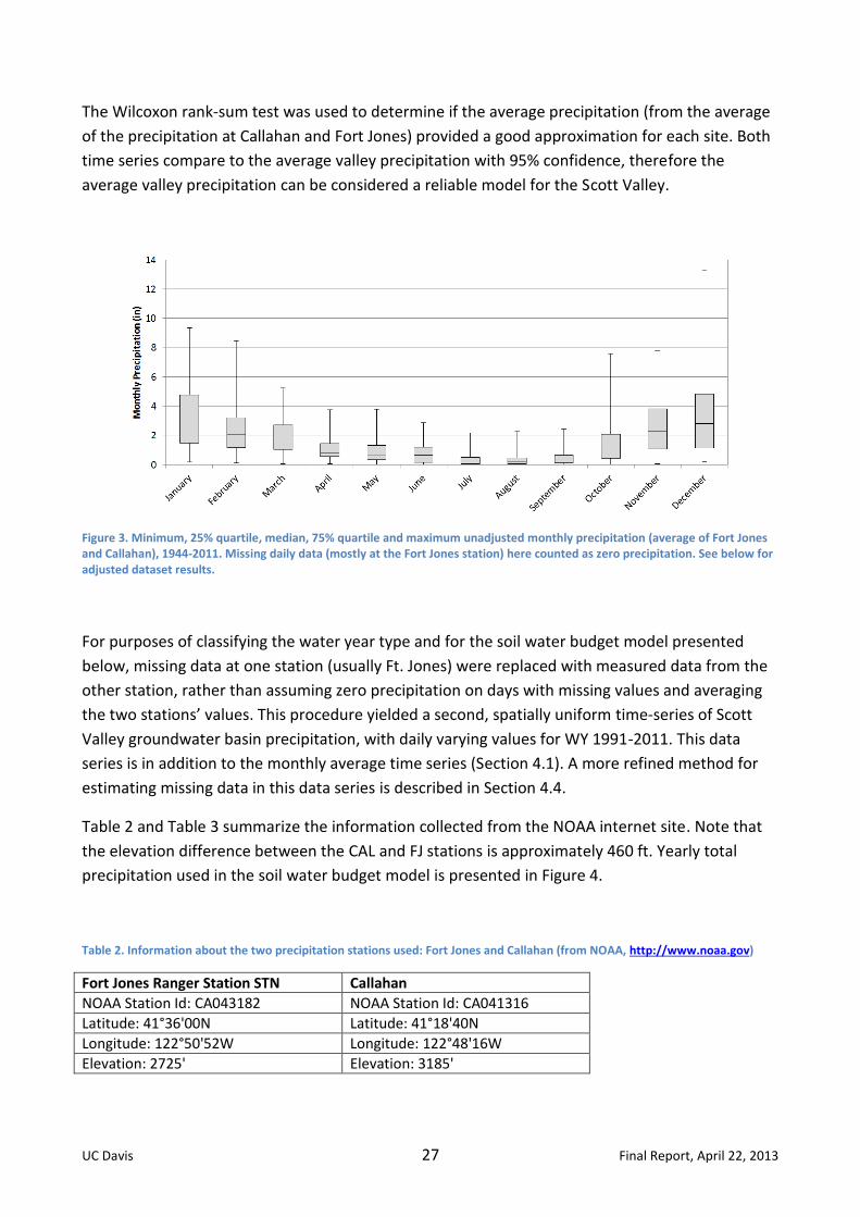
The Wilcoxon rank-sum test was used to determine if the average precipitation (from the average
of the precipitation at Callahan and Fort Jones) provided a good approximation for each site. Both
time series compare to the average valley precipitation with 95% confidence, therefore the
average valley precipitation can be considered a reliable model for the Scott Valley.
Figure 3. Minimum, 25% quartile, median, 75% quartile and maximum unadjusted monthly precipitation (average of Fort Jones and Callahan), 1944-2011. Missing daily data (mostly at the Fort Jones station) here counted as zero precipitation. See below for adjusted dataset results.
For purposes of classifying the water year type and for the soil water budget model presented
below, missing data at one station (usually Ft. Jones) were replaced with measured data from the
other station, rather than assuming zero precipitation on days with missing values and averaging
the two stations’ values. This procedure yielded a second, spatially uniform time-series of Scott
Valley groundwater basin precipitation, with daily varying values for WY 1991-2011. This data
series is in addition to the monthly average time series (Section 4.1). A more refined method for
estimating missing data in this data series is described in Section 4.4.
Table 2 and Table 3 summarize the information collected from the NOAA internet site. Note that
the elevation difference between the CAL and FJ stations is approximately 460 ft. Yearly total
precipitation used in the soil water budget model is presented in Figure 4.
Table 2. Information about the two precipitation stations used: Fort Jones and Callahan (from NOAA, http://www.noaa.gov)
Fort Jones Ranger Station STN Callahan
NOAA Station Id: CA043182 NOAA Station Id: CA041316
Latitude: 41°36'00N Latitude: 41°18'40N
Longitude: 122°50'52W Longitude: 122°48'16W
Elevation: 2725' Elevation: 3185'

UC Davis 28 Final Report, April 22, 2013
Table 3. Long-term historical averaged monthly precipitation and annual total for Fort Jones and Callahan in inches (from NOAA, http://www.noaa.gov). For this analysis, missing data at one station are replaced by the value measured at the other station prior to computing averages and totals.
Monthly Precipi-tation
Jan Feb Mar Apr May Jun Jul Aug Sep Oct Nov Dec Avg. Annu-
al Total
Fort Jones 3.72 2.95 2.43 1.34 0.95 0.67 0.42 0.58 0.74 1.22 3.26 3.52 21.8
Callahan 3.72 2.94 2.44 1.34 1.15 0.82 0.46 0.35 0.64 1.39 2.95 3.1 21.3
Figure 4. Precipitation in inches/year. One single value is used daily across the whole valley. For this analysis, missing data at one station are replaced by the value measured at the other station prior to computing averages and totals.
The adjusted precipitation data are used to recalculate year types. Our analysis principally relies
on the analysis presented in Deas and Tanaka (2006). We updated their analysis to also include
years 2005 through 2011. We recalculated the exceedance probability curve for the period 1936-
2011, then used the percentile thresholds suggested in Table 4 (here: Figure 5) of Deas and Tanaka
(2006), which identifies dry years, and then select these years in our 21 year modeling period,
from 1990 - 2011. Results are presented in Figure 6.
0
5
10
15
20
25
30
35
Pre
cip
itat
ion
, in
che
s/ye
ar
Year

UC Davis 29 Final Report, April 22, 2013
Figure 5. Expert judgment classification from Deas and Tanaka (2006), Table 4.
Figure 6. Analysis of precipitation to evaluate the year type.
Our results are in agreement with previous reports (Deas and Tanaka, 2005, 2006, 2009). The dry
and below normal years identified in our study period are (listed in order from most dry to less
dry): 2009, 1991, 2001, 1994, 1992, 2005, 2004, 2007, 2010, 2008, 2002, and 1993. The wettest
years in the WY 1991 – 2011 period are 2006 and 2003. This order is slightly different from that

UC Davis 30 Final Report, April 22, 2013
shown in Figure 4, since the year classification is based on October-March data and does not
include precipitation in April through September.
4.3 Precipitation - Watershed Method, Annual Average Total Precipitation
California Rivers Assessment (CARA) is a computer-based data management system designed to
provide access to information and tools with which to make sound decisions about the
conservation and use of California's rivers (http://endeavor.des.ucdavis.edu/newcara/). For the
Scott River Basin, CARA reports an average precipitation of 35.87 inches per year. The
precipitation coverage is represented in a precipitation map showing lines of equal rainfall
(“isohyets”) based on long-term mean annual precipitation data compiled from maps and
information sources at the USGS, the California Department of Water Resources, and the
California Division of Mines. Source maps are based primarily on National Weather Service data
for approximately 800 precipitation stations throughout California collected over a sixty-year
period (1900-1960). The minimum mapping unit is 1000+ acres and the isohyet contour intervals
are variable due to the degree of variation of annual precipitation with horizontal distance. The
CARA database utilizes a weighted average to determine a single value of mean annual
precipitation; the isohyet areas, after intersection, are multiplied by the average rainfall for each
isohyet-derived polygon and divided by the total area of the CARA watershed1.
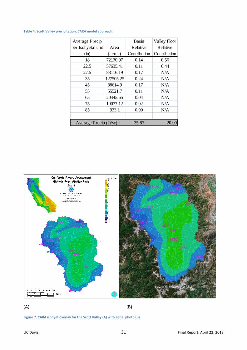
The CARA Model suggests an average precipitation of 35.87 in/yr across the watershed, much
higher than the 21.6 in/yr measured on the valley floor overlying the groundwater basin (see
Section 4.2). The CARA watershed area of the Scott Valley includes the high precipitation and
snowfall areas of the uplands and mountains. Spatial analysis of the CARA isohyet contour map
against a satellite image of the Scott Valley (Figure 7) shows that the valley floor overlying the
groundwater basin has average annual precipitation values of 18-22.5 inch isohyets. A spatial
analysis of the contributing isohyet areas (Table 4) yields an estimated yearly precipitation of 20 in
for the area overlying the Scott Valley groundwater basin comparable to the NOAA-derived
estimation (Table 3).
1 On 6/29/2012 the UC Davis Information Center for the Environment (ICE) was contacted to see how they created the
CARA model. The response from ICE suggested that the model was outdated and use of PRISM
(http://www.prism.oregonstate.edu/) or other more recent models would be more appropriate.
UC Davis 31 Final Report, April 22, 2013
Table 4. Scott Valley precipitation, CARA model approach.
(A) (B)
Figure 7. CARA isohyet overlay for the Scott Valley (A) with aerial photo (B).
Average Precip
per Isohyetal unit
(in)
Area
(acres)
Basin
Relative
Contribution
Valley Floor
Relative
Contribution
18 72130.97 0.14 0.56
22.5 57635.41 0.11 0.44
27.5 88116.19 0.17 N/A
35 127505.25 0.24 N/A
45 88614.9 0.17 N/A
55 55521.7 0.11 N/A
65 20445.65 0.04 N/A
75 10077.12 0.02 N/A
85 933.1 0.00 N/A
35.87 20.00Average Precip (in/yr)=

UC Davis 32 Final Report, April 22, 2013
4.4 Considering Spatial Trends in the Precipitation Modeling Method
NOAA has precipitation stations not only at Fort Jones (station ID USC00043182) and Callahan
(station ID USC00041316), but at two additional locations on the Scott Valley floor, at Greenview
and at Etna (Figure 2). As mentioned above, the Fort Jones data series is the longest, beginning in
1936, while Callahan data are available from 1943 to present. Other stations have significantly
shorter observation periods. The long historical datasets at Fort Jones and Callahan provide the
most representative view of the highly variable precipitation record compared to other stations.
But additional stations are valuable to determine possible spatial trends in precipitation patterns
across Scott Valley. Furthermore, missing values at the Ft. Jones station (and the few missing
values at the Callahan station are here replaced with statistically based estimates of the
precipitation on missing data days to obtain a more accurate record of daily, monthly, and annual
precipitation totals.
We use the NOAA precipitation data at all four Valley floor stations for further analysis and for
developing regression equations. First, data were inspected visually and extreme outliers were
removed. Then, with use of StatPlus®, the upper outlier boundary was calculated
(Outlier≥Q3+1.5*IQR, where IQR is the inner quartile range). The subsequent data analysis was
completed without those outling values.
The NOAA stations overlying the groundwater basin are located at Fort Jones, Callahan,
Greenview, and Etna. The Fort Jones and Callahan stations are discussed in sections 2.1 and 2.2.
The additional two stations are located in Etna and Greenview. Local residents report that
precipitation is generally lower near the eastside of the valley floor than the westside of the valley
floor. We used the additional precipitation records from Etna and Greenview to determine
whether the climate station data available within the area overlying the Scott Valley groundwater
basin are sufficient to verify such significant spatial trends..
Besides being of significantly less extent in time, the temporal resolution of the reported data
differs across the precipitation stations: the Fort Jones and Callahan stations report precipitation
values daily in 1/10th mm. The Greenview station reports precipitation values only as monthly
totals in 1/10th mm. The Etna station reports precipitation values hourly in 1/100th in.
We applied a linear regression analysis to reconstruct complete precipitation records for the Etna
and Greenview stations for 1943-2011, using StatPlus® software. The same regression procedure
was used to also fill in the few missing values in the Fort Jones and those in the Callahan records
during that time period. Separate regression equations were generated for each of twelve
calendar months. For each month of the year, separate regressions were generated for each of the
four stations against all other three station records (12 x 4 x [4-1] regression equations). At each
of the four precipitation stations, the three regression equations were ranked separately for each
of the twelve calendar months by their correlation coefficient. Missing daily precipitation data
were then computed using the highest ranked station-to-station specific regression equation for

UC Davis 33 Final Report, April 22, 2013
which data at any of the other three stations were available. For the Greenview station, regression
equations were used to generate daily data from monthly total reported precipitation.
Daily data from October 1990 to September 2011 were compared for spatial precipitation trends
across the Scott Valley groundwater basin. Over the 20 year study period, the average yearly
precipitation, computed from the annual totals during 1990-2011 for Callahan, Fort Jones, and
Greenview differed by less than 0.8 in (less than 4%), with values of 21.34, 22.05, and 21.27 inches
respectively. At the Callahan station, 88% of the yearly precipitation occurs from October to April,
while it is 90% at Fort Jones. Only about 2-inches of precipitation occur during the irrigation
season, most of which would likely not reach the groundwater basin.
The Etna station recorded an average annual precipitation of 27.98 inches, approximately 30%
higher than the other three stations. From Figure 7, we can see that the location of the Etna
station places it on the edge of the model extent along the western mountains, not unlike the
Greenview station.
To determine the quality of the estimated Greenview values, monthly precipitation from NOAA
was compared with estimated monthly totals of daily data obtained from the regression analysis
using a two sample homoscedastic t-test at alpha level 0.05. The test failed to reject the null
hypothesis H_0: µ_1=µ_2 (p=.05593), so we can conclude that the regression precipitation values
do not significantly differ from the NOAA values.
With all missing values at Greenview, Ft. Jones, and Callahan replaced by regression estimated
values (but not considering the Etna data series), the average annual precipitation across all three
stations, for WYs 1944-2011 is 21.3 in/yr, for WYs 1991-2011, it is 21.8 in/yr (Figure 11). In
comparison, the average annual precipitation at Ft. Jones and Callahan only, with missing values
replaced by estimated values, is 21.5 in/yr for WY 1944-2011 and 22.0 in/yr for WY 1991-2011,
consistent with the average annual precipitation obtained from the CDEC dataset of monthly
precipitation totals (see above). The precipitation data from the NOAA and CDEC online
repositories are very similar, but not quite identical due to different handling of missing values in
the aggregation of daily data to monthly data. They also differ in the time steps and measurement
units of the reported values. But for practical purposes, these differences are negligible.
The precipitation measured at the Etna station often differs markedly from the values measured at
the other stations, which prompted additional data analysis. In the 20 year period from October
1990 to September 2011, there are 167 days for which the difference between Etna and the
average valley precipitation, computed from the Fort Jones, Callahan, and Greenview data, is
greater than 0.5 inches. As shown in Figure 8A, Etna precipitation is frequently greater than the
average valley precipitation. Figure 8B shows the same comparison but only for cases when Etna
has precipitation exceeding 0.5 in. In some instances, Etna’s precipitation is two orders of
magnitude higher than the average valley precipitation. Of 167 days with differences exceeding
0.5 inches, only 40 days show Etna precipitation to be less than the average valley precipitation.
Thirty-nine days return a difference between Etna and the average valley value that is larger than
1 inch. Of these, Etna has the lower precipitation on only 10 days. Notably, on each day where

UC Davis 34 Final Report, April 22, 2013
Etna records a value that is more than 0.5 inches lower than the average, the Etna recording is 0
inches. It is therefore unclear, whether there are operating or local positioning biases to the Etna
data series.
(A) (B)
Figure 8. Etna precipitation compared to average Scott Valley precipitation. A: all Etna precipitation; B: only Etna precipitation exceeding 0.5 in.
Figure 9. Valley floor precipitation cokriging interpolation with anisotropy.
0.01
0.1
1
10
0.001 0.010 0.100 1.000 10.000
Etn
a P
reci
p (
in)
Avg Valley Precip (in)
0.01
0.1
1
10
0.001 0.010 0.100 1.000 10.000
Etn
a P
reci
p (
in)
Avg Valley Precip (in)

UC Davis 35 Final Report, April 22, 2013
Average annual total precipitation measured at Etna, Greenview, Fort Jones, and Callahan were
interpolated (using ArcGIS®) and mapped across the groundwater basin (Figure 9). We used
cokriging with large NNW-SSE anisotropy to map spatially variable precipitation across the valley.
The anisotropy reflects the hypothesized strong precipitation gradient across the West-East extent
of the valley. However, even if the Etna precipitation were considered relatively accurate, the high
precipitation at the western-most margin of the Scott Valley groundwater basin only affects a
relatively small area of the basin and would exclude the Greenview area. The Greenview station,
also on the westside of the Valley, agrees well with those at Callahan and Fort Jones.
While of nearly identical yearly averages, daily values at Greenview, Callahan, and Fort Jones
exhibit significant variance among each other, as would be expected across the significant extent
of the groundwater basin (25 miles long and up to 10 miles wide at its widest point). But given that
the integrated hydrologic model for which this data series is developed operates effectively at
monthly stress periods, a spatially averaged daily precipitation value, obtained from the relatively
complete Callahan and Fort Jones stations, is considered adequately representative of
precipitation dynamics across the Scott Valley groundwater basin.
In conclusion, using the four available precipitation stations, it was not possible to either support
or disprove the observation of a strong west-east gradient in precipitation totals reported by local
residents. Additional stations on the eastern margin of the Valley and on the Valley’s southwest
side would be needed to support these qualitative observations. Furthermore, the number and
location of the precipitation stations for which data were available, and the temporal extent of the
data currently do not justify a spatially distributed precipitation map for the groundwater basin.
Future precipitation gauges would be needed to enhance our understanding of orographic
precipitation mechanisms in the valley, which may lead to alternative rainfall estimates. Until such
additional data are available, daily precipitation across the entire Scott Valley groundwater basin is
assumed to be uniform, represented by the arithmetic average of the measured daily Fort Jones
and Callahan or at Fort Jones, Callahan, and Greenview, with missing data replaced by the
regression estimated data. This time series, developed from daily data, was used for the
streamflow regression analysis described in the next section.
The choice of uniform precipitation does not preclude future alternative approaches in the
integrated hydrologic modeling effort. Spatially variable precipitation, if additional data become
available, could be accommodated by the water budget model described in this report and hence
become part of a groundwater-surface water model.

UC Davis 36 Final Report, April 22, 2013
5 Streamflow
The Scott Valley groundwater basin and its overlying streams are fed by runoff from the
surrounding mountains. Tributaries to the Scott River, including the two forks of the Scott River
itself, emanate from the mountains carrying significant runoff.
Understanding groundwater-surface water interactions in the Scott Valley requires some
knowledge of the streamflow amounts that enter the valley floor overlying the groundwater basin.
In this section, we describe and investigate available data. We also construct time series of
streamflow in all major tributaries of the Scott River and for the South Fork and East Fork of the
Scott River, which join at the upper end of the Scott Valley floor. The main purpose for developing
these time series is to provide an approximation of surface flows into the Scott Valley as part of
the Scott Valley Integrated Hydrologic Model.
The eight tributaries of interest here are Sugar, French, Etna, Patterson, Kidder, Mill (a tributary to
Shackleford Creek), Shackleford, and Moffett Creeks. There are other tributaries to the Scott River,
but their flows tend to be ephemeral, relatively smaller, and their exact magnitude is not as critical
to understanding groundwater-surface water interactions in Scott Valley. In an integrated
hydrologic model, these may be represented as a diffuse source of recharge along the mountain
front around Scott Valley. The Scott River itself is gauged near Callahan at both the East and South
Forks (upstream of the confluence). An additional long-standing gauge (“Ft. Jones”) is located
downstream of Scott Valley, west of Fort Jones on the Scott River.
Location of the flow gauges has been provided by SRCD and is shown in Figure 10. The gauges at
Sugar Creek, Moffet Creek, and Kidder Creek are located above irrigation diversions and do not
reflect tributary inflows to the Scott River. Gauges at French Creek, South Fork, and East Fork are
located at the margin, but within the Scott Valley.
Most of the tributaries have very limited records of streamflow gauging, while the Ft. Jones gauge
has a complete record for the past seventy years (Figure 11). To develop an appropriate
groundwater-surface water model for the Scott Valley groundwater basin, it is therefore necessary
to also develop a model of the main stem and tributary streamflows, at the upgradient boundary
of the Scott Valley floor, for those time periods for which no streamflow data are available.
Here, we chose to determine missing tributary and main stem streamflow data at the upstream
margins of the groundwater basin through statistical regression analysis. A number of
independent predictor variables are considered for the regression analysis: streamflow of the
Scott River at the downstream Fort Jones gauging station, streamflow at the East Fork and South
Fork gauging stations in Callahan, streamflows on the tributaries when measured (Table 5),
precipitation data, temperature data, and snowpack data. The program R® was used to create
linear regression models with accompanying diagnostic plots (see Appendix A).

UC Davis 37 Final Report, April 22, 2013
5.1 Snow Water Content for Regression Modeling
Snow water content stations are located throughout the Scott Valley. The measurements
considered here are those taken in the month of April. The stations at Box Camp (BXC) and Marble
Valley (MBV) were not used since the snowmelt from these stations enters the Scott River
downstream (north) of the Scott Valley. For the model, the yearly average of the measured snow
water content at Middle Boulder 1 (MBL), Etna Mountain (ETN), Dynamite Meadow (DYM),
Swampy John (SWJ), and Log Lake (LOG) were used to aggregate across intra-watershed
variabilities and to obtain a representative dataset of the snow water content for the regression
analysis.
An additional snowmelt-related variable investigated here is the number of days in a given
calendar year (not water year), on which the temperature at Callahan exceeded 21℃. At this
temperature the entire watershed is under snowmelt conditions.
5.2 Precipitation for Regression Modeling
Daily mean precipitation computed from measured data at the Fort Jones, Greenview, and
Callahan stations for 1943 – 2011 (see Section 4.4) were used to compute the following additional
independent variables in the regression:
“MoPrecip”: sum of the average daily precipitation during the current month t
“PrevMoPrecip”: sum of the average daily precipitation during the prior month, t -1
“WYPrecip2Date”: sum of the average daily precipitation between the beginning of the current
water year (starting on October 1) and the beginning of the current month, t
“WYPrecip”: sum of the average daily precipitation for the entire water year, of which the current
month, t, is part (a model with “perfect foresight” because it includes information that represents
events in the future relative to the date of the estimated streamflow).
5.3 Flow Gauges
Daily mean discharge has been recorded at Scott River near Fort Jones CA (USGS 11519500) since
October 1, 1941 (Figure 11). This data is available at http://waterdata.usgs.gov/nwis, with average
daily values reported in cubic feet per second (cfs). For the regression, daily data were converted
to units of acre-feet per day (1.9835 AF/day equals 1 cfs). This dataset is the most robust of all the
streamflows in the Scott Valley. The published record has no missing daily flows. On some days,
data are estimated by the USGS, and then approved for publication. Because of the abundant data
available, the Scott River near Fort Jones flow was a major component of the regression model.
Table 5 lists the dates of available tributary streamflow data used for the regression analysis,
including the east and south fork of the main stem Scott River.
Tributary flow was downloaded from the Water Data Library
(http://www.water.ca.gov/waterdatalibrary/). The following list includes the code for each
tributary: Shackleford Creek near Mugginsville (F25484); Mill Creek near Mugginsville (F25480);

UC Davis 38 Final Report, April 22, 2013
French Creek at Highway 3 near Callahan (F25650); Sugar Creek near Callahan (F25890); Scott
River, East Fork, at Callahan (F26050); and Scott River, South Fork, near Callahan (F28100). Dates
for which data are available are listed in Table 5. Data are provided as average daily flows (cfs) and
were converted to units of (AF/day).
Daily data were used for the regression analysis. Complete sets of daily data with measured
values, when available, and with regression estimated values otherwise, were aggregated to
monthly totals (AF/mo) for each individual month in the time series.
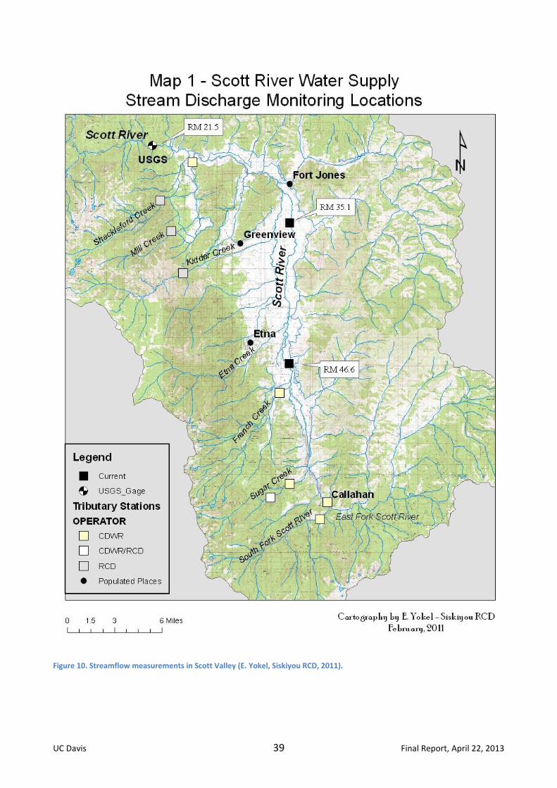
UC Davis 39 Final Report, April 22, 2013
Figure 10. Streamflow measurements in Scott Valley (E. Yokel, Siskiyou RCD, 2011).

UC Davis 40 Final Report, April 22, 2013
Figure 11. Log-transformed, normalized monthly average Scott River streamflow at Fort Jones, October 1941 through September 2011, computed from reported daily discharge (blue line). Water year total precipitation(green hanging bars) are computed as the average of measured and estimated daily precipitation data at the Fort Jones, Callahan, and Greenview stations (Section 4.4).
Missing data from the CDEC database are noted with a quality code of 160 or 255. Code 160
indicates that the flow was higher than the gage capacity, a situation for which it is difficult to
estimate an exact value. Similarly, the tributaries that are measured manually are measured only
under wadeable, non-flooding, conditions. Because many of the high value flows are missing from
the raw data, the regression models have difficulty replicating the peak flows. However, the goal
of the model is to understand the late summer/fall flows, which may affect fish, particularly
juvenile coho and fall-run Chinook salmon. Inaccurate prediction of high flow events is not
significantly affecting our analysis of late summer low flows. High flood flow may impact late
summer low flows indirectly – if at all - through groundwater recharge. Recharge from flood
events is difficult to predict, even if high flood flows were known precisely. While it is important
for the model to represent the streamflows accurately each month, more focus was therefore
placed on the accuracy of low flow events.
Table 5. Dates of available tributary streamflow data used for the regression analysis, including the east and south fork of the main stem Scott River.
0
20
40
60
80
100
120
140
160
180
200-3
-2
-1
0
1
2
3
ott
-41
ott
-43
ott
-45
ott
-47
ott
-49
ott
-51
ott
-53
ott
-55
ott
-57
ott
-59
ott
-61
ott
-63
ott
-65
ott
-67
ott
-69
ott
-71
ott
-73
ott
-75
ott
-77
ott
-79
ott
-81
ott
-83
ott
-85
ott
-87
ott
-89
ott
-91
ott
-93
ott
-95
ott
-97
ott
-99
ott
-01
ott
-03
ott
-05
ott
-07
ott
-09
WY
To
tal p
reci
pit
ati
on
(in
)
NO
RM
Sco
tt R
ive
r Fl
ow
(AF/
mo
)

UC Davis 41 Final Report, April 22, 2013
The degree to which unmeasured and poorly (under)predicted high flows may affect groundwater
recharge will need to be determined through sensitivity analysis with the integrated hydrologic
model.
5.4 Statistical Analysis: Streamflow Regression Methods
Monthly averages of reported daily streamflow data for the Scott River gauge at Fort Jones
and at the two gauges in Callahan are log-normally distributed. For the regression analysis, all
existing monthly average streamflow data, xi,t , at gauging station i and month (time) t were
therefore log-transformed and normalized to obtain a normally distributed data series of monthly
flows, Norm(xi,t), for each gauging station i:
( ) ( ) [ ( )]
[ ( )]
where M is the arithmetic mean (of the log-transformed data series xi) and STD is the standard
deviation.
Four transformed data series computed from known data sets were alternately used as
independent variables to build regression models of normalized log-transformed tributary flows
using linear regression:
“Norm(Scott)”: Norm(Scott River Flow at Fort Jones)
“ProductWeightedNorm(Scott)”:
√ ( )
“RatioWeightedNorm(Scott)”: ( )
√
“SumWeightedNorm(Scott)”: [Norm(Scott River Flow at Fort Jones) + WYPrecip +
WYPrecip2Date + MoPrecip + PrevMoPrecip + AvgSnowWC]
The following dependent variable time series were separately used against each of the above four
independent variables to build a number of regression models for comparison:
“Norm(Streamname)”: each individual normalized tributary flow gauge time series, all
times
“Norm(EastTribs)”: the combined record of all normalized tributary flow time series of
tributaries along the east side of Scott Valley, all times
“Norm(WestTribs)”: the combined record of all normalized tributary flow time series of
tributaries along the west side of Scott Valley, all times
“Norm(Tribs)”: the combined record of all normalized tributary flow time series, all times
To investigate seasonal biases in the regression models, the combined dataset of all normalized,
log-transformed tributary data, “CombinedTribs”, was dissected into
“Norm(Tribs-Season)”: season-of-the-year data (4 datasets) and

UC Davis 42 Final Report, April 22, 2013
“Norm(Tribs-Month)”: month-of-the-year data (12 datasets)
These 4 and 12 datasets were used to compute separate regressions for each season (fall: Oct-
Nov, winter: Dec-Feb, spring: Mar-Jun, summer: Jul-Sep) and separate regressions for each
calendar month (Oct through Sep), respectively.
Over the period of record, the normalized flow data for the Scott River show a significant shift that
occurs sometime during the long drought-free period between the 1955 drought and the 1977
drought. Beginning with the 1977 drought, summer month low flows (but not winter month high
flows) are significantly lower than in the 1955 drought and earlier. We therefore created another
set of regressions using a split “Norm(Tribs)” dataset:
Norm(Tribs)-Pre-WY1972, which includes WY 1943 to WY 1972, and
Norm(Tribs)-Post-WY1972, which includes WY 1973 to WY 2011 data.
Note that in the above lists, “tributary flow” and “tribs” include the South and East Fork of the
Scott River. For all of the above regressions, subsets of each log-transformed, normalized data
series were used for the time period of interest. However, across all analyses, the normalization of
each stream gauge’s dataset by its mean and standard deviation remains the same and is always
based on the total period of record for each stream gauge. In other words, we did not renormalize
the individual data series from original data for the particular time series used in the analysis,
neither for the independent nor for the dependent data series.
Additional regressions were implemented using the number of days in the calendar year to date at
which the temperature exceeded 21℃. This temperature was selected by computing the
temperature difference between Fort Jones and the highest point in the watershed, using the dry
adiabatic lapse rate (DALR). At 21℃, all of the surrounding snow-capped mountains have
temperatures above freezing, and they are contributing flow to the tributaries.
Goodness of fit was determined in a number of ways. First, the diagnostic plots from R were
visually examined. “Residuals vs Fitted” shows residual values as a function of the fitted value. If
the assumption of linear dependency between dependent and independent variable is justified,
these bounce randomly around the 0 line. If the results in the plot are closer together on one part
of the x-axis (e.g., the left side) than on the other part of the axis (where they would be more
spread apart or fanned out), then this would indicate a violation of the homogeneity assumption
that the residuals are independent of the magnitude of the predicted value. The “Q-Q plot” should
show linearity if the data are normally distributed. “Residuals vs. Leverage” should show no
pattern. “Scale-Location” plots should also show no patterns and issues of heteroscedasticity
would be noticeable through fan-like patterns in the plots.
5.5 Streamflow Regression: Results and Discussion
The regression slopes of the normalized tributary flows against the Scott River flows are all less
than 1 with a positive regression intersect (Table 6). This indicates that the geometric mean flows
of the tributaries have a tendency to occur when the Scott River below Ft. Jones is at less than

UC Davis 43 Final Report, April 22, 2013
geometric mean flow; and the low flow on the tributaries tend to be less extreme than on the
Scott River, or the high flows are not as extreme as on the Scott River, or both (relative to the
standard deviation). The only exception is Moffett Creek, which has regression slope slightly larger
than 1 with a slightly negative regression intersect.
The behavior observed on most tributaries is even more exaggerated when the normalized data
are separated into a pre-WY1972 and post-WY1972 series: prior to (and including) WY 1972,
tributary geometric mean flow occurs at approximately the Scott River geometric mean flow, with
the slope being slightly larger than 1 (high flows and/or low flows on the tributaries tend to be
slightly stronger than on the Scott River). After WY1972, tributary geometric mean flows occur
when the Scott River is at less than geometric mean flow and the extreme events (highs or lows or
both) are less exaggerated on the tributaries than on the main stem of the Scott River below Ft.
Jones: the log-transformed flows on the tributaries vary only at 84% of the relative variation on
the main stem below Scott Valley. Separating the time-series into two series, however, yields an
only slightly better correlation coefficient, r2.
Fitting each tributary separately against the Scott River data, or fitting the combined west side
tributaries separately from the combined east side tributary data also does not produce a much
higher correlation coefficients (Table 6). It therefore appears that a single regression for the
combined dataset of normalized, log-transformed tributary flows is adequate and also takes
advantage of the information that may be collected on some tributaries but not at others, given
that tributary flows are highly correlated among each other.
When weighting the regressions by additional information, two models emerge with correlation
coefficients similar to (and not much higher than) the unweighted regressions: the product-
weighted regression and the sum-weighted regression. The ratio-weighted regression, on the
other hand, performed very poorly.
The product-weighted regression provides large weights when high flow events coincide with wet
years and large snow pack, and low weights when low flow events coincide with dry years and
small snow packs. The product-weighted regression implies that tributary flows are relatively
smaller (compared to Scott River flows) in dry years with low snow pack than in average or wet
years or in years with higher snowpacks.
The sum-weighted regression provides the best correlation coefficient, if only slightly better than
the unweighted correlations. The sum-weighted correlation assigns additional weights to several
precipitation and snow-pack related data. But that does not significantly improve the predictive
capability, if the Scott River dataset alone was used.
In the Q-Q plot, most models showed some tailing off the line y=cx for low x values. Also, some
trends appear in residuals. For many regressions against Norm(Scott) and
SumWeightedNorm(Scott), the correlation coefficient, r2, is larger than 80% (Table 6) indicating an
overall strong, but not perfect, goodness of fit. R-squared can give an approximate indication of
how well the estimated data fit the measured data overall, but it is important not to base all

UC Davis 44 Final Report, April 22, 2013
judgment on this value alone. Some models had r2 larger than 70%, yet failed to model the high
and low streamflow values well.
A visual comparison of the plotted estimated and actual values was made (see Appendix A). This
method of determining goodness of fit was the best way to see how well the regression modeled
the flow, especially the important summer/early fall flow.
Mill, Etna, and Patterson were difficult to analyze since these tributaries were only gauged for one
year. With so few points to compare, it is difficult to tell which regression provides the best fit. To
be conservative, the regression that shows the best for the other tributaries should also be used
for these three flows.
Table 6. Key regression slopes, intersects, and regression coefficients. Availability of data from individual streams is listed in Appendix (also see Table 5).
Dependent Variable Independent Variable
Regression Slope [-]
Regression Intersect [-]
r2 [%]
Norm(Tribs) Norm(Scott) 0.903 0.122 81.2
Norm(Tribs)-Pre-WY1972
Norm(Scott) 1.053 -0.000405 84.7
Norm(Tribs)-Post-WY1972
Norm(Scott) 0.840 0.218 82.4
Norm(WestTribs) Norm(Scott) 0.881 0.205 81.4
Norm(EastTribs) Norm(Scott) 0.964 0.00975 83.7
Norm(Kidder) Norm(Scott) 0.804 0.129 76.7
Norm(Shackleford) Norm(Scott) 0.952 0.243 89.9
Norm(Sugar) Norm(Scott) 0.979 0.0406 83.0
Norm(Moffett) Norm(Scott) 1.044 -0.0567 78.0
Norm(EastFork) Norm(Scott) 0.941 0.0364 87.4
Norm(SouthFork) Norm(Scott) 0.900 0.317 82.1
Norm(French) Norm(Scott) 0.879 0.350 82.2
Norm(Tribs-Summer) Norm(Scott) 0.758 -0.123 50.1
Norm(Tribs) RatioWeighted-Norm(Scott)
18.66 0.14 37.0
Norm(Tribs) ProductWeighted-Norm(Scott)
0.1118 0.006066 76.3
Norm(Tribs) SumWeighted-Norm(Scott)
0.930 0.370 82.3
Norm(Tribs) SumWeighted-Norm(Scott) – Pre-
WY1972
1.111 0.240 85.6
Norm(Tribs) SumWeighted-Norm(Scott) – Post-
WY1972
0.876 0.682 83.7
For the best fit, we were particularly interested in matching flows during the low flow season, if
not perfectly, then at least such that flows are over-predicted in some years and under-predicted
in other years. Ideally, the regression would have zero bias, where bias is here defined as

UC Davis 45 Final Report, April 22, 2013
Bias = Norm(Trib)actual - Norm(Trib)predicted
Bias was calculated separately for each calendar month and each tributary for the time period of
record, using two example regressions. Data are not available in all months to compute bias (Table
7 - Table 10).
Comparing prediction results between various regression methods, qualitative differences in the
overall pattern of fit are small compared to the large annual variations in streamflow. Weaknesses
in one prediction are repeated, at slightly better or worse levels, in other predictions.
A large number of negative bias occurs during the summer months at the East Fork, in particular.
Visual inspection of predicted vs. measured time series indicates that predicted values for the
earlier time period at the East Fork seemed to have a particularly significant bias, not being able to
predict the low flows in most summer months. While the East Fork has significant bias, especially
for September’s low flows, no adjustments were made to correct this bias or any other stream’s
bias. Not enough month-specific data are available to correct for potential bias.
For the pre- and post-1972 regressions (Norm(Tribs)Pre-WY1972, Norm(Tribs)Post-WY1972),
streams had at most 13 datapoints, and commonly much less (Table 7-Table 10).
From the many individual regressions, we found that those regressions that included all tributaries
in the equation provided a better fit overall than the regressions for individual tributaries, or the
regressions for individual months or individual seasons.
The regressions of normalized tributary streamflows vs. RatioWeightedNorm(Scott) provided the
relatively poorest fit (r2 < 0.4), although some summer flows are better predicted than by other
models. A much better correlation was obtained when computing a regression of tributary flows
vs. ProductWeightedNorm(Scott) (r2 =76.3%). Commonly, this regression, however, tends to
significantly underestimate peak flows and overestimate low flows.
In summary, of the many regression models developed, two regression models stood out as
having a significant better fit, particularly in the critical low-flow season: Norm(Tribs) vs
Norm(Scott) and Norm(Tribs) vs SumWeightedNorm(Scott).
The best fit was obtained by the split time period regressions, Norm(Tribs)Pre-WY1972 and
Norm(Tribs)Post-WY1972 vs. SumWeightedNorm(Scott), particularly in the critical summer
months. Splitting the regression gave slightly better results (r2 values of 84.7% and 82.4%) than the
fully combined regression Norm(Tribs) vs. SumWeightedNorm(Scott) (r2=81.2%). The split
regression model would also provide the best possible fit for the flows at Mill, Etna, and Patterson
given the lack of raw streamflow data for these tributaries. The regression is considered
particularly good, given the large variability in flow volume and geographical range within the
valley. The split Norm(Tribs)Post-WY1972 vs. SumWeightedNorm(Scott) and the split
Norm(Tribs)Post-WY1972 vs. Norm(Scott) will be the best candidates for use in the groundwater-
surface water model.

UC Davis 46 Final Report, April 22, 2013
Table 7. Regression bias for Norm(Tribs)- Pre-WY1972 vs. SumWeightedNorm(Scott). White areas indicate that data are available to compute a bias for those months.
Table 8. Regression bias for Norm(Tribs)- Post-WY1972 vs. SumWeightedNorm(Scott). White areas indicate that data are available to compute a bias for those months.
Table 9. Regression bias for Norm(Tribs)- Pre-WY1972 vs. Norm(Scott). White areas indicate that data are available to compute a bias for those months.
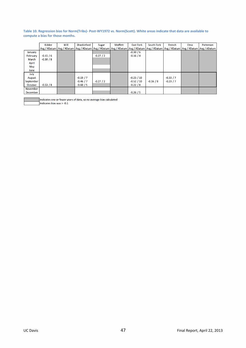
UC Davis 47 Final Report, April 22, 2013
Table 10. Regression bias for Norm(Tribs)- Post-WY1972 vs. Norm(Scott). White areas indicate that data are available to compute a bias for those months.

UC Davis 48 Final Report, April 22, 2013
6 Evapotranspiration and Crop Coefficients
Evapotranspiration was calculated using a program designed at UC Davis, the NWSETO program
(Snyder, 2002). The NWSETO program is used to calculate reference evapotranspiration (ET0) for
short grass. The atmospheric inputs for this program include, for each month, average maximum
daily temperature, average minimum temperature, maximum and minimum humidity, wind
speed, and percent cloud cover. The NWSETO program provides two alternative reference ET0
values based on either the Penman-Monteith (1965) or based on the Hargreaves and Samani
equations (1982). The calculated ET0 obtained from the climate records and NWSETO were
compared and evaluated on the basis of observed values available for Scott Valley as discussed
below, prior to using it within the water budget model. The two sets of data were generally in
agreement. For this study, the ET0 values calculated by NWSETO using the Hargreaves and Samani
equation have been used.
Crop coefficients (kc) and ET0 are used to estimate specific crop evapotranspiration rates. The kc is
a dimensionless number (usually between 0.1 and 1.2) that is multiplied by the ET0 value to obtain
an estimate of the actual crop ET (ET). The estimate of actual crop ET is primarily designed to help
an irrigation manager schedule irrigation frequency and amount, but is here used to estimate
actual crop ET for simulating a daily soil water budget. Crop coefficients vary by crop, stage of
growth of the crop, and by some cultural practices. Coefficients for annual crops vary widely
throughout the season, with a small coefficient in the early stages of the crop (when the crop is
just a seedling or, in the case of alfalfa, has been recently cut) to a large coefficient when the crop
is at full cover (the soil completely shaded).
Crop coefficients have been assigned as follows:
alfalfa: kc = 0.95 (Steve Orloff and Blaine Hanson, University of California, personal
communication) from February 15 to November 15, and kc=0 for the remainder of the
winter months. In alfalfa, a constant kc value is used for two reasons: first, the growing
period of alfalfa broadly coincides with that of the reference crop; secondly, alfalfa cuttings
do not occur at the same time across the entire study area. A time-varying kc value that
reflects individual cutting events on individual fields would require knowledge (or
simulation) of individual field cutting events over the period of interest. That level of detail
in the spatio-temporal variability of field-by-field water budgets was deemed not critical
for the current modeling effort. Also, using a slightly different growing period, such as
March 1st- October 31st would not significantly change the final ET value because the ET in
February and March is almost negligible. Simulations yield a 1990-2011 average annual ET
in alfalfa of 1,200 mm (39.4 inches), very close to the field values measured by Blaine
Hanson (Hanson et al., 2011a);
grain (wheat, barley, oats and triticale): we use a daily varying kc according to UCCE Leaflet
21427. Leaflet 21427 lists crop coefficients for two crops similar to the “grain” category
here: summer barley in Northern California Mountain Valleys and small winter grain in the
Sacramento Valley. The following is a combination of “barley” for “Mountain Valleys”

UC Davis 49 Final Report, April 22, 2013
(planting date: 4/30, harvest date: 8/31) with the “small grain” for “Sacramento Valley”
(planting date: 12/16, harvest date: 8/04) supported by the recommendation provided by
Steve Orloff and general information provided by the GWAC:
o planting date A: March 15, kc=0
o early season date B: April 20, kc=0.27
o mid season start date C: May 15, kc=1.15
o mid season end date D (after 70% of the 127 day period or 90 days): June 15,
kc=1.15
o harvest date E, July 20, kc=0
The daily kc values vary linearly between the above dates and values.
pasture: kc = 0.9 as suggested by the UCCE Leaflet 21427 for grazed pasture statewide, and
confirmed by Steve Orloff. To account for winter frost, we set kc=0.9 from February 15 to
November 15, but zero over the winter (same as for alfalfa).
natural vegetation: kc = 0.6

UC Davis 50 Final Report, April 22, 2013
7 Soils
The Soil Survey Geographic (SSURGO) Database, maintained by the Natural Resources
Conservation Service (NRCS), was used to obtain spatial and tabular soils data for our project area.
This database contains soil attributes, which describe variables such as texture, particle size or
water holding capacity. We used information from this database to evaluate water holding
capacity (WHC) for each of the land use polygons delineated by the California Department of
Water Resources (DWR). The recommendation by UC Cooperative Extension personnel was to use
a root-zone depth of 4 ft (122 cm) to compute WHC. Available information in the SSURGO
database was WHC to 100 cm and to 150 cm. To simulate WHC at the recommended depth of 4 ft
(122 cm), we mapped WHC for both 100 cm and 150 cm in each soil map unit, then obtained the
WHC used for the soil water budget simulation using an area-weighted average of all intersecting
soil type polygons and their WHCs at 100 cm and at 150 cm within each DWR land use polygon
(Figure 12). For modeling purposes, the same root zone depth was assumed for all crops. In
practice, grain and alfalfa are do not have the same rooting depth; however, a sensitivity analysis
of the root zone depth, presented later in the report, shows that doubling the root zone depth
does not significantly affect results. Selecting a uniform root zone depth for both crops in the soil
water budget model is therefore a reasonable assumption.
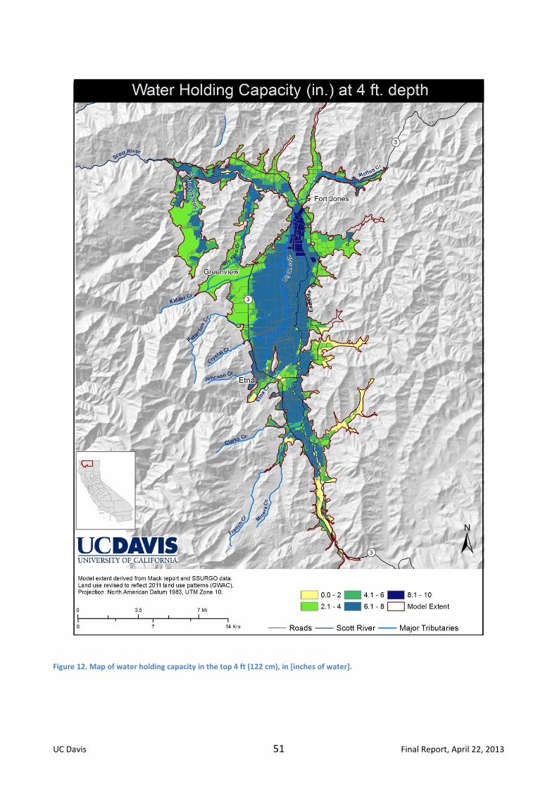
UC Davis 51 Final Report, April 22, 2013
Figure 12. Map of water holding capacity in the top 4 ft (122 cm), in [inches of water].

UC Davis 52 Final Report, April 22, 2013
8 Groundwater
8.1 DWR Well Log Review
The main focus of our well log analysis was on identifying geologic structure within the Scott
Valley alluvium and on identifying the location of irrigation (agricultural) wells, regardless of
whether these were active or inactive. Well locations are used in the water budget model to
represent groundwater pumping required to meet agricultural water demands in wells nearest to
each field, when not met by surface water supplies.
A scanned copy of all well logs available for the Scott Valley and immediately surrounding areas
was obtained from the California Department of Water Resources (CDWR). An extensive review of
these 1,701 well logs was conducted in order to gain a better understanding of the hydrogeology
of the valley. Well logs typically provided information on the well’s location, on geologic facies
encountered during drilling, albeit at varying degrees of description detail and accuracy, and for
some wells the logs provided information on the hydrologic characteristics of the well, including
specific capacity or pumping data. Well logs also indicated the major use of the well. Our review
included the following:
Domestic Wells: 1,302
Irrigation Wells: 240
Industrial Wells: 3
Public/Municipal Wells: 4
Other (Monitoring, Test, etc.): 152
The number of wells identified to be in or near the Scott Valley was 598 wells. The number of wells
located within the Version 2 model boundaries and included in our GIS database is 406 wells:
Domestic Wells: 192
Irrigation Wells: 182
Other: 32
Well logs were first geo-located throughout the integrated hydrologic modeling area (see below)
using a variety of information. The primary information used was the parcel number of the
property where the well was situated. This information was typically provided on the well log
itself. Parcel numbers and associated locations for the Scott Valley area were obtained from the
Siskiyou County Assessor’s Office files. The second datum used for geo-locating a well was the
well owner and address listed on the well log. If neither of these two methods obtained a location
match, the well logs were categorized by their township/range/section information, which was
obtained by reviewing the well location sketch provided by the driller, and from a review of aerial
photography to identify the parcels where the wells are situated. Additionally, a field survey was
conducted throughout the valley to verify well locations where accessible or viewable from public
access places.
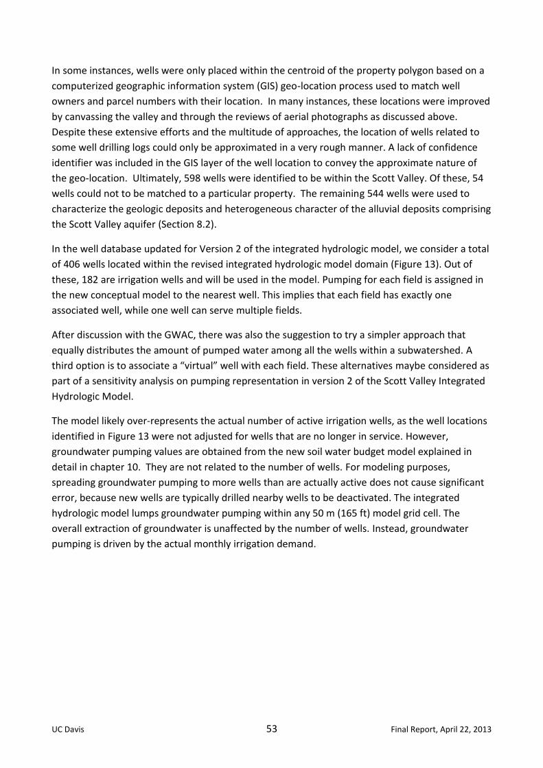
UC Davis 53 Final Report, April 22, 2013
In some instances, wells were only placed within the centroid of the property polygon based on a
computerized geographic information system (GIS) geo-location process used to match well
owners and parcel numbers with their location. In many instances, these locations were improved
by canvassing the valley and through the reviews of aerial photographs as discussed above.
Despite these extensive efforts and the multitude of approaches, the location of wells related to
some well drilling logs could only be approximated in a very rough manner. A lack of confidence
identifier was included in the GIS layer of the well location to convey the approximate nature of
the geo-location. Ultimately, 598 wells were identified to be within the Scott Valley. Of these, 54
wells could not to be matched to a particular property. The remaining 544 wells were used to
characterize the geologic deposits and heterogeneous character of the alluvial deposits comprising
the Scott Valley aquifer (Section 8.2).
In the well database updated for Version 2 of the integrated hydrologic model, we consider a total
of 406 wells located within the revised integrated hydrologic model domain (Figure 13). Out of
these, 182 are irrigation wells and will be used in the model. Pumping for each field is assigned in
the new conceptual model to the nearest well. This implies that each field has exactly one
associated well, while one well can serve multiple fields.
After discussion with the GWAC, there was also the suggestion to try a simpler approach that
equally distributes the amount of pumped water among all the wells within a subwatershed. A
third option is to associate a “virtual” well with each field. These alternatives maybe considered as
part of a sensitivity analysis on pumping representation in version 2 of the Scott Valley Integrated
Hydrologic Model.
The model likely over-represents the actual number of active irrigation wells, as the well locations
identified in Figure 13 were not adjusted for wells that are no longer in service. However,
groundwater pumping values are obtained from the new soil water budget model explained in
detail in chapter 10. They are not related to the number of wells. For modeling purposes,
spreading groundwater pumping to more wells than are actually active does not cause significant
error, because new wells are typically drilled nearby wells to be deactivated. The integrated
hydrologic model lumps groundwater pumping within any 50 m (165 ft) model grid cell. The
overall extraction of groundwater is unaffected by the number of wells. Instead, groundwater
pumping is driven by the actual monthly irrigation demand.

UC Davis 54 Final Report, April 22, 2013
Figure 13. Map of the irrigation type and of the available irrigation wells for Version 2 of the integrated hydrologic model. Locations have been refined by inspection (see text) and may not coincide with those reported by the California Department of Water Resources. The irrigation type reflects recent (2011) conditions. The year of conversion from “Other Sprinkler” (typically wheelline) to “Center Pivot” is an attribute of the “Center Pivot Sprinkler” polygons, if the conversion occurred after 1990, and is taken into account in the soil water budget model.

UC Davis 55 Final Report, April 22, 2013
8.2 Geologic Heterogeneity
The well logs obtained from DWR revealed a tremendous amount of heterogeneity within the
alluvial deposits of the Scott Valley. A preliminary geostatistical analysis of the geologic
heterogeneity was performed using the so-called transition probability approach (Carle and Fogg,
1996). The transition probability approach is a modified indicator variogram analysis that
describes the joint probability distribution of a discrete set of hydrogeologic or geologic facies
groups throughout the aquifer system. The transition probability is defined by:
a) a finite number of facies, typically the three to five most common facies observed
in a set of geologic records (well logs), e.g., coarse-grained stream deposits,
coarse-to-fine grained overbank deposits, and fine-grained flood-plain deposits.
One of these facies (usually the facies with the largest volumetric proportion) is
designated as “background facies”.
b) The volumetric percentage of each facies within the aquifer system of interest.
c) The mean lengths (average straight-distance extent) of all but the background
facies in the dip, strike, and vertical direction.
d) The juxtapositional preference among the facies sequence, in other words, the
likelihood that one particular facies is located adjacent to another particular
facies with a probability that is significantly higher or lower than that obtained if
the facies are randomly assembled.
Within the context of groundwater modeling, the transition probability analysis provides a
quantitative analysis of the geologic heterogeneity encountered in a groundwater basin. It also
provides the simulation framework for generating equally-probable, random realizations of the
highly heterogeneous aquifer architecture, conditioned to the specific well logs at the locations
where these are available. These random realizations can also be conditioned to surficial geologic
information available in soils maps (Weissman, 1999). The more concrete information available,
the more specific the random realizations of the aquifer architecture (less variability between
individual realizations).
To illustrate the geologic heterogeneity of the Scott Valley, a single realization of the Scott Valley
aquifer was generated with the geostatistics software T-PROGS. T-PROGS utilizes the transition
probability method, a modified form of indicator kriging, through calculation of transition
probability measurements, modeling spatial variability with Markov Chain models, and conditional
simulation of the well log information. In this context, the term “indicator” is used to denote
categorical classification of aquifer sediments (e.g., coarse, intermediate, fine), as opposed to
continuum values (numeric values, for example, hydraulic conductivity varying log-normally with a
mean of 20 feet per day and a standard deviation of 10 feet per day).
The T-PROGS geostatistical analysis was based on the information obtained from the 544 wells
that were geo-located in the valley. Following a review of these well log records, it was
determined that three geologic facies would be modeled: clay or fine-grained sediments, sand,
and gravel. As such, in one-foot vertical increments, the data from the well logs was interpreted

UC Davis 56 Final Report, April 22, 2013
as one of the three listed facies, and transition probability statistics were calculated including
mean length, proportion, and transition probabilities. Within the combined digitized well logs, a
total of 3,982 geologic facies transitions were recorded in the vertical direction (z-direction).
In order to complete the analysis, a review of the SSURGO soil mapping of the ‘C Horizon’ soil
(approximately 0.1 to 0.15m below ground surface) was undertaken to provide information on the
nature of the lateral variability observed in geologic deposits. Each deposit identified by the
SSURGO mapping (in the subreport entitled Wind Erosion Prediction System Related Attributes)
was interpreted as one of the three facies chosen for analysis using at least one of the following
indicators: percentage of silt/clay versus sand, and grain size analysis provided to determine
between sand and gravel. If the percentage of silt and clay was greater than 50%, the texture was
considered to be clay. This particular limit was chosen as it fit the qualitative description of
deposits described as loam, clayey-loam, or clay. If the percentage of sand was greater than 50%,
the texture was considered to be either sand or gravel with the fragment descriptor being the
parameter deciding between the two. If the fragment percentage was greater than 40, the gravel
indicator was selected. Also, in a few instances the description was “stratified sandy loam and clay
loam”. In these cases, sandy loam was chosen as the key layer depending on overall percentages.
This seemed to match descriptions of gravel material versus sandy loam. If sandy loam was the
description of the material, it was generally labeled as belonging to the sand fraction.
For the geostatistical analysis of the soils information, the deepest soil horizon profile was used.
For example, most of the soils were given a description to a depth of approximately 150 cm (5 ft),
split between at least two soil horizons: the upper soil horizon less than 50 cm (1.7 ft), and at least
one deeper horizon which was typically close to 100 cm (3 ft) in depth. Often, the data for this
deeper soil horizon were incomplete and only included the percentage of clay. In these cases, the
information provided was often descriptive but sufficient to make a determination of the category
to which the soil belonged (clay/sand/gravel).
To complete the analysis, the soil maps had to be discretized so that mean lengths, proportions,
and transitions could be calculated. In previous applications, cross-sections of arbitrary
discretization were used to accomplish the analysis. For this study, a 50 m by 50 m grid was used
to discretize the soil map (not including the tailings area in the southern Scott Valley). In GIS, the
grid was overlain on the soil map, and a Spatial Join operation was completed so that each model
grid node was provided with a single soil type. This Spatial Join was completed based on the soil
type with the highest percentage of area within the grid cell (as calculated by the GIS function).
Essentially, the process allowed for 621 horizontal (rows) and 420 vertical (columns) cross-sections
to be evaluated as input data. Once discretized, the transition probability data was calculated,
including mean length, proportion, and transition for each of three facies.

UC Davis 57 Final Report, April 22, 2013
Figure 14. Vertical transition probability curves obtained from an analysis of 544 wellbore logs located within the study area in Scott Valley.
The results of the data analysis show the relative proportions of deposits and display the differing
mean lengths of deposits in each of the ordinal directions. The above transition probability curves
represent important aspects of the geologic facies deposits (Figure 14). The curves for each type
asymptotically approach the value that represents the proportion of each facies deposit. From the
z-direction analysis, the proportions of each facies obtained are 51% for clay, 37% for gravel, and
12% for sand. Similar proportions arose from the analysis of the soils map in the XY lateral plane,
with proportions of 61% for clay, 28% for gravel, and 11% for sand. Furthermore, in the above
transition probability diagram, one can draw a tangent along each auto-transition curve and
extend the tangent to the x-axis. The value at which the tangent intersects the x-axis represents
the mean length of the particular facies. The mean lengths of each deposit in the z-direction
obtained from this analysis were 15.0 m (49 ft) for clay, 12.7 m (42 ft) for gravel, and 10.1 m (33 ft)
for sand. The mean lengths of each deposit in the X direction (east-west cardinal directions) were
1,379 m (4,524 ft) for clay, 755 m (2,477 ft) for gravel, and 640 m (2,099 ft) for sand.

UC Davis 58 Final Report, April 22, 2013
The results of the transition probability analysis above were used as input for a Markov-chain
random field generator (included in the TPROGs software package) to generate random, equi-
probable aquifer structure conditioned on the geologic facies information available for Scott
Valley, obtained from the well logs (representative of the vertical dimension) and the soils maps
available for Siskiyou County (representative of the lateral dimensions). Figure 15 represents one
such realization created with the T-PROGs software with a discretization of 10 ft vertically, 500 ft
in the x (W->E) direction and 1,000 ft in the y (S->N) direction. It should be noted that any number
of realizations can be created, and although each one will be different, they all will have similar
“patterns” with all realizations having the same overall proportion of each geologic facies,
determined from the z-direction analysis, and the same mean lengths and juxtapositional
preference in each of the three directions. At the surface and along well locations, each
realization will preserve the actually known data.
Figure 15. TPROGS Realization of the Scott Valley geologic deposits. Length units are in feet. The image shows a hypothetical aquifer volume that is approximately 100 ft thick, 6 miles in the x direction and 25 miles in the y direction. Note that this image is stretched in the X-direction relative to the y-direction and it does not consider the actual boundaries of the Scott Valley aquifer. It is shown only to conceptually illustrate the heterogeneity encountered in the alluvial deposits of Scott Valley.
While the realization shown in Figure 15 is random, it has important features to note that are
shared by all realizations and that are indicative of the overall patterns in the Scott Valley aquifer
architecture: the facies exhibit somewhat preferential, elongated connectivity in the y (north-
south), but less connectivity in the x direction (east-west), a pattern that represents observations
z(ft)
x(ft)
y(ft)

UC Davis 59 Final Report, April 22, 2013
in the well logs and in the soil map. It is also obvious from the above illustration that the gravel
deposits, which are the hydraulically most conductive facies within the aquifer, are highly
connected throughout the aquifer system and not isolated from one-another by clay-layers or clay
walls. In particular considering that gravel and sand make up approximately half of the aquifer
sediments, the connectivity of these coarser-grained sediments is very high and it appears unlikely
that significant proportions of sand and gravel would be completely isolated from the regional
aquifer system (i.e., encased and surrounded completely by clay). They are likely well-connected
to the main-stem of the Scott River.
On the other hand, a review of the boring logs in certain areas shows that a clay layer exists over
portions of the valley. This realization as well as hand-drawn cross-sections of the valley created
from boring logs, show that these clay layers or lenses may not be broad enough to act as a true
confining features. As such, portions of the aquifer may be semi-confined, where they are located
below a local clay layer or a clay lens that is relatively broad in extent. However, a spatially
extensive confined aquifer does not appear to be present in the Scott Valley. We also note that no
sand and gravel has been recorded below about 76 m (250 ft) depth in the few existing logs that
exceed such depth.
The geostatistical realization of the Scott Valley aquifer indicates that the Scott River, which
intersects with the surficial layer of this aquifer model, is alternately passing along finer and
coarse-grained sediments. It is important to keep in mind, however, that this model was created
with a lateral resolution of 150 m (500 ft) and also largely depends on the resolution and surveying
detail of soil mapping units, which is typically on the order of several hundred meters. The above
illustration therefore ignores variability that inevitably occurs at scales smaller than about 150 m –
300 m (500 ft – 1,000 ft).
The analysis here provides an initial survey of spatial variability in the Scott Valley groundwater
system. Spatial variability, such as that shown in Figure 15 may be incorporated into future
groundwater models, after further analysis of well logs, additional review of streambed sediment
studies not reviewed here, and perhaps an improved geostatistical assessment of facies variability
in the alluvial system. However, Version 2 of the Integrated Hydrologic Model will not yet include
such detailed hydrogeologic facies representation.

UC Davis 60 Final Report, April 22, 2013
9 Watersheds, Land Use, Irrigation, and Land Elevation
A variety of data were used to create input for the model. The model extent was determined
based on the extent of groundwater storage units outlined by Seymour Mack in 1958 (Mack,
1958), while the land use data were derived from the California Department of Water Resources
(DWR) Land Use survey data. The most recent land use data for Siskiyou County available from
the DWR is from the 2000 DWR land use survey. Although a more recent land use survey has been
completed by CDWR in 2010, the processed data were not available for use in our project. Since
the modeling period is 1990 -2011, the 2000 land use survey was used as the basis upon which we
developed the spatial component of our model.
9.1 Model Boundaries and Subwatersheds
Our study area boundaries were selected to represent the Scott Valley area containing surficial
alluvial deposits. To delineate these areas in a digital map, a spatial analysis was performed and
we assumed that the extent of the alluvium was defined largely by the absence of steep
topographic gradients (more than 3%). A digital elevation model (DEM), derived from National
Elevation Data (NED), was created and topographic gradients (slope) were computed. The DEM
with slopes was then draped over 2005 National Agriculture Imagery Program (NAIP) color aerial
imagery, and used as a visual guide to manually digitize the contiguous areas of the Scott Valley
that have a three percent slope or less.
The Scott Valley model area covers approximately 50,000 acres. It is subdivided into nine
subwatersheds for purposes of modeling surface water supplies and the distribution of these
supplies within subwatersheds (Table 11, Figure 16). The subwatersheds are Scott, French, Etna,
Patterson, Kidder, Moffet, Mill, Shackleford, and the Scott River Tailings. These subwatersheds
were created partly based on the water storage units delineated by Seymour Mack in his 1958
report. Crystal and Patterson Creek are combined into a single subwatershed. Similarly, Johnson
and Etna Creek are combined into a single subwatershed. Other smaller subwatersheds are
included with larger ones (Figure 16).
Mack (1958) and our Scott Valley model Version 1 data work did not include the Scott River
Tailings subwatershed located in the upstream part of the valley. For Version 2 of the Scott Valley
Integrated Hydrologic Model, the southern tailings area of the Scott Valley is included in the
analysis and in the groundwater flow domain. From visual field inspection, it appears that the
tailings aquifer consist primarily of large boulders, with very high hydraulic conductivity and rapid
connectivity to the stream. During the late summer and fall low flow season, the Scott River, at the
surface, is often disconnected across this highly permeable subwatershed.

UC Davis 61 Final Report, April 22, 2013
Table 11: Total areas of subwatersheds (Figure 16), total area for various irrigation types (Figure 13), total area for various irrigation water sources (Figure 19), and total area of land use (Figure 18), in acres. All values represent 2011 conditions. Note that not all acreage in the alfalfa/grain and pasture category is irrigated.
Subwatershed Name Area
(acres) Irrigation
Type Area
(acres) Water Source Area
(acres) Land Use Area
(acres)
Etna Creek 4,223 Non-irrigated 18,549 DRY 3,356 Water 166
French Creek 501 Flood 10,864 GW 16,526 Alfalfa/Grain 17,421
Kidder Creek 9,298 Sprinkler 12,564 MIX 3,949 Pasture 16,578
Mill Creek 2,237 Center Pivot 6,928 SUB 2,106 ET/No Irrig. 14,151
Moffett Creek 2,437 Unknown 1,107 SW 7,596 No ET 1,695
Patterson Creek 4,032 None/unknown 16,478
Scott River 20, 736
Scott River tailings 3,562
Shackleford Creek 2,984
Study Area Total 50,011 Total 50,011 Total 50,011 Total 50,011
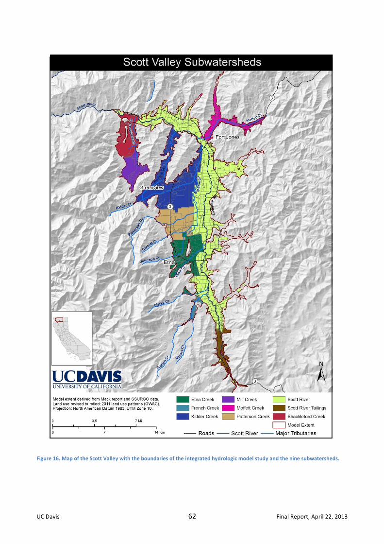
UC Davis 62 Final Report, April 22, 2013
Figure 16. Map of the Scott Valley with the boundaries of the integrated hydrologic model study and the nine subwatersheds.

UC Davis 63 Final Report, April 22, 2013
9.2 Land Use Categories
The CDWR land use surveys delineate polygon shapes identifying areas with various types of land
use (i.e. residential, commercial, agriculture). We used the existing year 2000 land use database,
which also includes attributes such as irrigation type, water source, and expanded the database to
include values that describe water holding capacity, and soil hydraulic conductivity for each land
use polygon. Using extensive feedback from the Scott Valley Groundwater Advisory Committee
(GWAC), we confirmed or updated the water source, irrigation type and land use associated with
each polygon. Feedback was provided by the GWAC and local landowners through marked up
large maps that reflect the knowledge of local landowners about dominant 2000 – 2011 conditions
and changes in irrigation type, water source, and land use that have occurred since the DWR
survey in 2000. It is assumed that the feedback effectively reflects conditions in 2011 and the
years immediately preceding 2011.
It is important to note that some of the feedback provided on land use, water source, and
irrigation type reflects an outright correction of the CDWR 2000 landuse map (i.e., reflects year
2000 conditions as well as year 2011 conditions), some reflects land use changes since the year
2000 survey. For modeling purposes, we did not make a distinction between these two types of
suggestions. However, the most important irrigation type change is that from sprinkler irrigation
to center pivot irrigation due to the efficiency increase. That specific change was explicitly tracked
in the land use database by adding a conversion date to those polygons that are in center pivots in
2011. The dynamics of that change are reflected in the soil water budget model (see below). With
these dynamics simulated explicitly, and with the overall feedback from the GWAC and local
landowners, the resulting landuse, irrigation type, and water source map is considered more
representative of 1991 – 2011 conditions than the CDWR 2000 map. No changes were made to the
shape of individual land use polygons defined in the CDWR 2000 survey.
We aggregated the land use polygons into four main categories each of which reflects a common
water demand:
1. new “alfalfa/grain rotation” land use category: all land use parcels in this category are
assumed to be on an alfalfa-grain rotation. Since we do not have exact data on the
rotation, we simulate the rotation by creating an eight-year cycle. Each field in this
category is randomly assigned one of the eight years in the cycle during which it goes into
“grain” rotation. All other years, a field is assumed to be in “alfalfa” land use. Each year,
one out of eight fields is in “grain” and the rest are “alfalfa”. The same eight-year rotation
is followed throughout the simulation period (1990-2011). This new land use category
includes the following CDWR land use classes:
a. grain ( wheat, barley, oat, triticale)
b. corn
c. alfalfa, mixed alfalfa/orchardgrass
d. rice
e. sudan
f. miscellaneous truck crops

UC Davis 64 Final Report, April 22, 2013
2. new “pasture” land use category. This includes the following CDWR land use classes:
a. pasture
b. highwater pasture
c. improved pasture
d. mixed pasture
e. grass
f. cemeteries
g. lawns
h. institutions
i. schools
j. residential
k. recreation
l. nursery
3. new land use category “ET without irrigation” representing pasture-like ET (crop
coefficient, kc = 0.6) but without irrigation. This includes:
a. natural vegetation
b. natural highwater meadow
c. misc. deciduous trees
d. trees
4. new land use category “no ET and no irrigation” for all land uses without ET (kc = 0) and
without irrigation (but with recharge from precipitation via soil moisture storage). This
includes:
a. barren
b. commercial
c. dairy
d. extractive industry
e. farmsteads
f. industrial
g. livestock feedlots
h. municipal
i. paved
j. storage
k. trailers
l. unpaved
m. vacant
Figure 17 presents the updated land use map using a lumped land use categorization scheme
based on the definition of land use categories also used in the CDWR 2000 map. Figure 18 shows
the same land use map after re-categorization into the newly assigned four land use categories as
listed above. Both maps reflect the changes suggested by the GWAC. The new land use categories
of Figure 18 are used in the water budget model development. A separate, fifth landuse category

UC Davis 65 Final Report, April 22, 2013
is comprised of 166 acres of open water areas (streams, lakes, wetlands) within the study area
(Table 11).
Figure 17. Land use categories based on DWR 2000 map and updated for 2011 using suggestions from GWAC and local landowners.
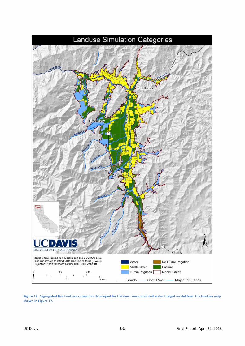
UC Davis 66 Final Report, April 22, 2013
Figure 18. Aggregated five land use categories developed for the new conceptual soil water budget model from the landuse map shown in Figure 17.

UC Davis 67 Final Report, April 22, 2013
9.3 Irrigation Type and Irrigation Water Source
Irrigation types were derived based on the DWR categories and summarized in three groups for
modeling purposes as follows:
“surface flood irrigation” consists of the following CDWR categories:
o iB - border flood irrigation: the correspondent water source is surface water, mix or
sub-irrigation (per June 2011 GWAC meeting, this is the same as wild flooding)
o iF - furrow irrigation: it applies only to a few small fields, often now in center pivots
with groundwater as water source for irrigation
o iW - wild flooding: the correspondent water source for irrigation is surface water or
sub-irrigation
“center pivot sprinkler irrigation” consists of the following CDWR categories:
o iC - center pivot: typically with groundwater as water source for irrigation
o others that were converted to center pivot sometime in the last 20 years, with
dates and prior crop specified in the new land use polygon table
“other sprinkler irrigation” consists of the following CDWR categories:
o iH - handmoved sprinkler irrigated
o iR - wheel-line sprinkler irrigated
Unknown irrigation type affects 1107 acres (Table 11), of which 27 acres are classified as pasture
and the remainder (1080 acres) as alfalfa/grain. In addition, 700 acres of alfalfa/grain and 1,861
acres of the pasture category, mostly residential land use in the original DWR classification (e.g., in
the Ft. Jones and Etna area) are classified as non-irrigated in the year 2000 CDWR land use survey.
In total, 18,549 acres are not irrigated within the study area, with or without ET.
The irrigation efficiency values used in the water budget model have been fixed based on
suggestions from Steve Orloff and the GWAC. As a future modeling task, we will use irrigation
efficiency as a calibration tool to check against the irrigation scheduling suggested by the GWAC.
The values used in the model are:
surface flood irrigation: 0.70 (Steve Orloff, 2011, oral communication)
center pivot sprinkler: 0.9 (Steve Orloff, 2011, oral communication)
other sprinkler irrigation: 0.75 (Steve Orloff, 2011, oral communication)
Irrigation water sources are represented in Figure 19 and are summarized in Table 11 as:
Groundwater (GW)
Surface water (SW)
Subirrigation (SUB)
Mixed surface water-groundwater (MIX)
Dry (DRY)
None/unknown/other

UC Davis 68 Final Report, April 22, 2013
There are no known water sources on 177 acres of alfalfa/grain and on 475 acres of pasture, and
on practically all open water and other unirrigated land uses (with or without ET).
Figure 19. Water source assigned to each polygon, based on data from the CDWR Land Use, 2000, and based on revisions suggested by the Scott Valley GWAC (2011).
UC Davis 69 Final Report, April 22, 2013
9.4 LiDAR Land Surface Elevation Data Analysis
LiDAR data, published by Watershed Sciences, Inc. (2010) and obtained from the NCRWQB in
2012, were used to create a bare earth digital elevation model of the Scott River area.
Because Light Detection and Ranging (LiDAR) data are typically of higher resolution than National
Elevation Data (LiDAR is sub-meter accuracy while NED is available in three to 30 meter
resolution), they provide a more accurate digital elevation model.
This high resolution bare earth DEM was then used to create a digitized model of the Scott River
thalweg. Draped over the 2005 NAIP color aerial imagery, the bare earth DEM was categorized
into 10 centimeter classifications, which showed the river channel morphology in great
detail. Using the aerial imagery as a guide, the Scott River thalweg was digitized in ArcGIS, with a
vertex placed every 1/3 of a meter. Elevation values from the bare earth DEM were then assigned
to each of these vertices in ArcGIS. Average slope between vertices were also calculated in ArcGIS.

UC Davis 70 Final Report, April 22, 2013
10 Soil Water Budget Model - Methods
10.1 Introduction and Overview
We have developed a soil water budget model that serves to define the spatio-temporal
distribution of groundwater pumping, surface water diversions, groundwater recharge, and
evapotranspiration throughout the Scott Valley. The soil water budget model computes spatially
and temporally varying water fluxes across the approximately 50,000 acre study area. The spatial
resolution is variable and equal to the individual fields and land use units (polygons) identified by
the 2000 CDWR land use map, which has been updated (Figure 17), and converted into five major
land use categories (Figure 18). In time, the model operates on daily information values, primarily
driven by available climate and streamflow data resolution and the need to properly represent soil
water storage dynamics. For surface water accounting purposes, the model domain is subdivided
into nine major subwatersheds (Figure 16).
The field soil water budget method is a simple root zone bucket model at each land use polygon as
described below. This model, however, does not represent a complete surface water budget of
the Scott Valley, since it does not account for river-groundwater interaction or evapotranspiration
off shallow water-table from non-irrigated crops or natural landscapes, or from open water
surfaces (the latter being the “Water” land use category in Figure 18). The complete surface water
budget will be considered when this model is coupled to the MODFLOW groundwater-surface
water model which is under development.
The output from the soil water budget model is a 21 year time-series (1990-2011) of daily surface
water diversions, pumping, irrigation, evapotranspiration, and recharge values at each land use
polygon except those designated as “Water”. The model also computes the theoretical irrigation
deficiency, defined as the difference between optimal crop evapotranspiration and actual
evapotranspiration. Using a daily time-step for the soil water budget model allows us to account
for the often rapid dynamics in soil moisture and for carry-over storage of soil moisture for later
plant evapotranspiration.
In contrast, the integrated hydrologic model will be driven by monthly stress periods, which means
that pumping and recharge are constant within a month. For the integrated hydrologic model,
daily water fluxes from the soil water budget model will be aggregated for each month to provide
monthly, land use polygon specific recharge, pumping, evapotranspiration, and surface water
delivery values. The monthly stress periods in the integrated hydrologic model reflect the
generally slower dynamics of groundwater flow. However, if warranted, the budget model
described here can also be applied to an integrated hydrologic modeling scenario with weekly or
bi-weekly varying stress periods or to stress periods of varying period length.
The conceptual approach is largely derived from the approach taken for Version 1, but has been
revised in close collaboration with UC Cooperative Extension personnel, the Scott Valley GWAC,
and technical experts familiar with the Scott Valley. Some of the key differences between the

UC Davis 71 Final Report, April 22, 2013
revised Version 2 soil water budget model and the earlier (unpublished) Version 1 soil water
budget model include:
daily rather than monthly time-step
soil moisture storage changes in the soil root zone are tracked
the southern part of Scott Valley with the tailings is included in the model domain
revised and updated land use map and land use categories are used
irrigation schedules and irrigation demands have been revised
Whereas the previous soil water budget model (Scott Valley Integrated Hydrologic Model Version
1) was compiled in a spreadsheet, the new soil water budget model has been developed and
compiled as a Fortran program, which allows for more efficient control on various conceptual
model scenarios and inclusion of soil water budget model variables in model sensitivity and
calibration procedures. The development of this code and its linkage to a GIS database provides us
with the capability to include detailed spatial information, readily adjust for newly available
information from local parties, and provides flexibility to generate a multitude of future simulation
scenarios.
10.2 Description of the Soil Water Budget Model
10.2.1 Model Input Preparation
The following data have been compiled in the previous sections to provide input for the soil water
budget model:
climate (digital climate station records)
o precipitation
o potential evapotranspiration
streamflow
o daily streamflow data on all tributaries including main stem forks
o subwatershed delineation
land use:
o crops with crop coefficient
o irrigation method
o irrigation water sources
soil properties (digital USDA soil maps with properties)
o water holding capacity
hydrogeology
o location of pumping wells
Each land use polygon in the Scott Valley is characterized by a set of properties (or attributes)
mainly derived from the GIS analysis:
Land use, divided into the five main categories as described above (Figure 18): 1)
alfalfa/grain rotation with seven years of alfalfa followed by one year of grain, 2) pasture

UC Davis 72 Final Report, April 22, 2013
(including some urban landscapes, see above), 3) evapotranspiration without irrigation
(includes natural vegetation, natural highwater meadow, misc. deciduous trees, trees), and
4) no evapotranspiration and no irrigation with recharge from precipitation via soil
moisture storage (barren, commercial, dairy, extractive industry, municipal, industrial,
paved, etc); 5) water surfaces (mostly streams), which are not included in the soil water
budget model, but will be part of the integrated hydrologic model.
Soil type derived water holding capacity (Figure 12). The model is assuming a root-zone
depth of 4 ft (8 ft in the sensitivity analysis described below).
Irrigation type (Figure 13): flood, center pivot, or sprinkler; some fields switch from flood or
sprinkler to center pivot at some field-specific date between 1991 and 2011, based on
review of historic aerial photos.
Water source (Figure 19): groundwater “GW”, surface water “SW", subirrigated “SUB”,
mixed groundwater-surface water “MIX”, and farming without irrigation “DRY”.
However, the alfalfa/grain land use and the pasture land use include areas for which either the
irrigation type is not known or the water source is not known or both (Table 11). For the soil
water budget model, the following assumptions are made to account for all potential
combinations of land use, irrigation type, and water source:
If the land use is either alfalfa/grain or pasture, and:
a) water source is GW, MIX, or SW, but the irrigation type is unknown (480, 2, and 335 acres,
respectively): assume that the irrigation type is “other sprinkler irrigation”;
b) water source “DRY” or “SUB”, but the irrigation type is unknown (200 and 34 acres,
respectively): treat the land use as “ET without irrigation”;
c) irrigation type is unknown and the water source is unknown (56 acres): assume that the
irrigation type is “other sprinkler irrigation” and the water source is GW;
d) irrigation type is “center pivot” or “other sprinkler” or “flood”, but the water source is
unknown (177 acres of alfalfa/grain and 475 acres of pasture): assume that the water
source is GW;
e) irrigation type is “non-irrigated”, regardless of water source (700 acres of alfalfa, 1861
acres of pasture land use, mostly in residential areas): treat the land use as “ET without
irrigation”. This includes 484 acres of alfalfa/grain and 1275 acres of pasture classified as
having a “DRY” water source; and 10 acres of pasture classified as having a “SUB” water
source. No or unknown water source is specified for 120 acres of non-irrigated alfalfa/grain
and for 469 acres of pasture land use.
These assumptions may not accurately reflect the irrigation type or water source in all cases, but
due to the relatively minor acreage of these special cases, the above simulation process is a
representative simplification that does not significantly affect the outcome of the soil water
budget model.
UC Davis 73 Final Report, April 22, 2013
10.2.2 Tipping Bucket Approach for Soil Water Budget Modeling
The soil water budget calculations are performed using a tipping bucket approach. The main
concepts associated with the tipping bucket approach here are the following:
The simulation starts with the beginning of water year 1991, on October 1, 1990 and is
performed daily.
We assume that the initial soil water content on October 1, 1990 is zero, since the starting
point is after the completion of the irrigation season (the soil water profile fills during the
first winter months).
We assume that adjusted daily precipitation (Padj) is the portion of daily precipitation (P)
that infiltrates into the soil and is available for daily evapotranspiration (ET) or recharge:
o if P > 0.2*ET0, Padj(i) = P
o if P <= 0.2*ET0, Padj(i) = 0 (FAO Bulletin 56)
o ET0 is the daily reference evapotranspiration (FAO Bulletin 56)
This effectively assumes that precipitation events of less than 20% ET0 on any given day will
sit on leaves or bare ground and evaporate before the end of the day, without affecting soil
water storage, plant evapotranspiration, etc. For all soil water budget computations, we
use adjusted precipitation and not precipitation. Adjusted precipitation is the same across
the valley, since we only use one ET0 value.
With daily time-steps, the tipping bucket approach used to calculate daily soil moisture storage
changes and deep percolation in each polygon can be expressed as follows:
Theta (i) = max(0, theta(i-1) + Padj(i) + Irrig(i) –actualET(i) –Recharge(i)) Eq. 1
Recharge (i) = max(0, theta(i-1) + Padj(i) + Irrig(i) –actualET(i) – WC4(i)) Eq. 2
Where:
Theta(i) = water content at the end of day i
Padj(i) = precipitation on day i
Irrig(i) = irrigation on day i
ET(i) = evapotranspiration on day i= ET0*crop_coefficient
Recharge (i) = deep percolation to groundwater
Actual ET(i) = min (ET(i), theta(i-1) + Padj(i) + Irrig(i)) Eq. 3
Groundwater recharge is defined here as the amount of soil water that cannot be held against
gravity, i.e., the amount of soil water that is above the water holding capacity, WC4, of the root
zone in the land use polygon at the end of each day. The model does not account for the time
delay between water leaving the root zone and water reaching the water table at the top of the
groundwater system. Given that water table depth is generally less than 20 ft and that recharge
values are aggregated monthly for the integrated hydrologic model, the assumption of

UC Davis 74 Final Report, April 22, 2013
“instantaneous recharge” is justified, but can be evaluated as part of a sensitivity analysis with the
integrated hydrologic model.
The above algorithm intrinsically exerts complete mass balance control on each land use polygon:
Padj(i) + Irrig(i) – actualET(i) – Recharge(i) = theta(i)-theta(i-1) Eq. 4
Furthermore, we can compute deficit irrigation for each polygon as follows:
Deficiency(i)= ET(i) – actualET(i) Eq. 5
10.2.3 Irrigation Water Source Simulation
Where does the irrigation water, Irrig(i), come from? The source of the irrigation water depends on the water source and land use specified for an individual land use polygon.
For pasture, irrigation water typically is supplied by surface water. Groundwater pumping
in pasture occurs only for polygons where the GIS land use coverage indicates that
irrigation water is being sourced fully or partially from groundwater (“GW” or “MIXED”, see
below).
Alfalfa/grain land use polygons can be irrigated with surface water, groundwater, or a mix
of surface water/groundwater. Based on information from the GWAC, the distinction
between “SURFACE WATER” and “MIXED” water source was ignored, and all alfalfa/grain
fields with “SURFACE WATER” source were treated as if equipped for a “MIXED” source: in
either case, alfalfa/grain is always fully irrigated. First with surface water and when surface
water allocations dry up, groundwater is used for irrigation.
The simulated decision process that leads to a land use polygon switching from surface water
irrigation to groundwater irrigation can be summarized as follows:
Total monthly discharge rates in the Scott River and in its tributaries at the entry into the
Scott Valley are obtained for each of the nine subwatersheds as calculated by the
regression analysis (chapter 5).
Within each subwatershed and for each month, the surface water used for irrigation by
each polygon is subtracted from the total monthly discharge of the respective
subwatershed stream in a given month.
Once the total irrigation demand within a subwatershed, in a given month, exceeds
(estimated) stream discharge, and if the field is alfalfa/grain, then groundwater is used to
make up the difference between surface water available and the irrigation demand. The
available amount of surface water is distributed to all polygons designated for use of
surface water at equal water depth (water volume proportional to polygon size). For each
polygon, the difference between surface water supply and irrigation demand for a given
month with surface water shortage is obtained by groundwater pumping.

UC Davis 75 Final Report, April 22, 2013
Canal losses to groundwater are currently not considered separately. Effectively, these are
included in the irrigation efficiency concept and therefore contribute to diffuse landscape
recharge.
The surface water delivery and groundwater pumping rates are driven by irrigation schedules and
by precipitation and evapotranspiration. Urban and domestic pumping for irrigation of lawns, golf
courses, cemeteries, etc. is included in the soil water budget model, but allocated to nearby
agricultural wells. Domestic and urban water use other than for domestic/urban/residential
irrigation is currently neglected in the soil water budget model, but can be accounted for in the
MODFLOW groundwater-surface water model. Domestic/urban water use other than that used for
lawn/garden irrigation in Scott Valley is only a very small fraction of total water use in the Scott
Valley.
In the current water budget calculations, we apply an irrigation management scheme in which
irrigation is driven by crop ET and available precipitation (see below for details).
Recharge occurs across the entire integrated hydrologic modeling domain, either from irrigation
and rainfall, or from rainfall only (non-irrigated land uses).
10.2.4 Irrigation Management and Scheduling Simulation
The irrigation simulation is based on irrigation efficiency and evapotranspiration as the drivers for
computing applied water demand. It is based on the concepts developed for the CDWR
Consumptive Use Program (Orang et al., 2008). Irrigation amount is calculated using the same
approach for alfalfa, grain, and pasture, but the irrigation scheduling and irrigation demands differ
depending on three variables: crop type, irrigation type, and water source. Details of the irrigation
management model are described here. Note that land use designated as “Water” is not
associated with recharge, irrigation, evaporation, groundwater pumping, or surface water
deliveries.
1) Alfalfa/grain and pasture
Following the literature (FAO publication 56) for alfalfa, irrigation in each polygon k starts on the
first day i on or after March 25th when the soil water content has dried to less than 45% of field
capacity:
Theta(i) < (1-0.55)*WC4(k) Eq. 6
The depletion factor 0.55 is from FAO Publication 56, Table 22.
The last alfalfa irrigation application occurs on September 5th (typically it ends prior to the 3rd
cutting which is anytime between the last week of August and the 3rd week of September.
According to GWAC, few fields are irrigated after Labor Day). It is important to note that these
“irrigations” are not simulated as individual events but are spread evenly across the irrigation
season, i.e., the irrigation demand is computed daily based on the crop water demand (see
below).

UC Davis 76 Final Report, April 22, 2013
For grain, the first irrigation on a field k is determined exactly as for alfalfa but the earliest
potential starting date is March 15th. However, the last day of continuous irrigation on grain is
simulated to be much earlier than in alfalfa, on July 10th, after which the grain is harvested.
For pasture, the irrigation season is always from April 15th through October 15th (184 days).
However, on pasture that is surface water irrigated (which represents most pasture), no irrigation
occurs once surface water supplies become unavailable (the explanation of when surface water is
considered unavailable is presented above). When applied, irrigation is applied continuously
based on daily ET demand (again, we do not distinguish individual irrigation events).
The approach chosen here for simulating irrigation assumes that fields are all irrigated with the
same, irrigation type-specific irrigation efficiency. This represents a simplification of reality, where
some fields are relatively over-irrigated (mainly pasture fields) and others are relatively under-
irrigated. However, the irrigation efficiencies are chosen to represent average irrigation
management practices, given the irrigation type. The approach here also neglects irrigation non-
uniformity within individual fields. Large non-uniformity with significant under-irrigation in some
parts of the field may effectively increase field-scale irrigation efficiency.
For each polygon j and for each day i, the daily irrigation amount is calculated as shown in eq. 7
based on the evapotranspiration of the crop, adjusted for precipitation and considering the
irrigation efficiency of the crop:
Irrig_j(i)=(1/irrigation_efficiency_j)*(Max(0, (ET_j(i)-Padj(i)) Eq. 7
Where:
ET_j(i) = Kc_j* ET0(i) where Kc is the crop coefficient,different for each crop
Padj(i) is the adjusted precipitation on day i (Eq. 4)
For the soil water budget model, we assume that there is no contribution to evapotranspiration
from groundwater. Groundwater contribution will be thoroughly evaluated once the integrated
hydrologic model is developed, calibrated and coupled to the soil water budget model. This may
require an iterative coupling process between the integrated hydrologic model development and
the soil water budget model development.
2) ET/no irrigation category
The main assumption in this land use category is that, at all times:
Irrig(i) = 0
ET in this land use category is computed separately by two models: the soil water budget model
and the groundwater flow model (MODFLOW).
In the first step, we use the soil water budget model to compute daily ET (on day i):
ET(i) = kc* ET0(i) = 0.6 * ET0(i)
UC Davis 77 Final Report, April 22, 2013
With the additional constraint that ET(i) <= Theta(i-1) + Padj(i)
This latter constraint is the key difference to an irrigated crop: here, ET is constrained to the
naturally available water.
In a second step, ET that is due to direct uptake from the water table will be computed with the
groundwater flow model (MODFLOW with the evapotranspiration, ET, package). The MODFLOW
ET package uses root zone depth and maximum possible crop ET as input parameters.
The recharge is computed as indicated in the soil water budget model (Eq. 2, section 5.1). Note
that recharge is computed without consideration of ET directly from the water table. This means
that recharge may occur even if the water table is in the root zone. This conceptual dilemma
results from the fact that:
recharge computation is done prior to MODFLOW and is an input to MODFLOW
direct ET from the water table is computed as part of the MODFLOW simulation
Effectively, the explicit coupling of these two components will not have much influence on the
result, as water mass is still conserved by not allowing the sum of the two ET values (soil water
budget model and MODFLOW) to be larger than the optimal ET from this land use category (0.6 *
ET0). Note that this simulation process only applies to non-irrigated ET land uses.
3) No ET / no irrigation category
Land use categories of this type have neither irrigation nor evaporation, or evapotranspiration
from plants:
Irrig(i) = 0 at all times
ET(i) = 0 at all times
In the polygons within this category, we assume that runoff is negligible and that therefore
recharge is equal to the adjusted precipitation:
Recharge (i) = Padj(i)
10.3 Calibration of Reference Evapotranspiration (ET0)
Due to the sparse amount of observed data, calibration of the soil water budget model alone (i.e.,
not yet coupled to the groundwater MODFLOW model) is very difficult. Some values of reference
ET and ET were provided by Hanson et al. (2011a) and have been used for a hand-calibration of
the ET component used in the model.
Reference ET (ET0) for the soil water budget model has been calculated with the NWSETO program
developed at UC Davis, which is based on the Hargreaves and Samani (1982) equation. The

UC Davis 78 Final Report, April 22, 2013
reference ET values are summarized in Table 12 for the years 2007-2010 and are compared against
reference ET values calculated with the Hargreaves equation (Hargreaves et al., 1985).
Table 12 Reference ET (Seasonal Reference ET) calculated with the Hargreaves equation (Hargreaves et al., 1985) (modified from Hanson et al., 2011a) and obtained with the NWSETO program used here (Hargreaves and Samani, 1982).
Year
NWSETO calculated
values (in)
ET0 values (March 15-October 1)
with Hargreaves eq. (in)
2007 40.12 44
2008 39.48 42.6
2009 40.4 40.4
2010 38.12 37.4
ET0 (March 15-October 1)
The reference ET( ET0) values calculated with the NWSETO program overall were in agreement
with the reference ET values based on the Hargreaves equation (Table 12).
With the above reference ET values, crop evapotranspiration (which we call ET, as mentioned
above) is calculated as:
ET=kc*ET0
where ET0 is the reference ET described above and kc is the crop coefficient.
Observed values of alfalfa ET in Scott Valley were also available (Hanson et al., 2011a) and have
been compared with the calculated values.
As shown in Table 13 , observed and calculated alfalfa ET values for the period March 15-October
1 are in agreement for three of the years considered: 2007, 2009 and 2010. The values for 2008
are in disagreement because of a significant number of smoke days that occurred in June-July
2008 and are not accounted for in the NWSETO-based ET estimate.
Table 13 Measured and calculated ET values for alfalfa using a crop coefficient kc =0.95 . Measured values were obtained from Hanson et al., 2011a, Table 2).
Crop coefficient for Alfalfa= 0.95
Year
Calculated values
with kc=0.95
Measured values
(March 15-October 1)
2007 38.11 38.3
2008 37.34 29.4
2009 38.48 38.8
2010 36.13 36.03
* values for 2008 are expected to be lower than other years because of the numerous smoke days
ET (March 15-October 1)

UC Davis 79 Final Report, April 22, 2013
11 Soil Water Budget Model: Results
This section presents the results of the soil water budget analysis. Results are compared against
irrigation, evapotranspiration and recharge data available from relevant literature and against
data provided by the local GWAC.
The water budget simulation provides daily, field-by-field land use polygon specific outputs for all
of the following variables, which are aggregated to provide yearly and long-term average rates by
polygon, by land use, and by subwatershed:
1. Pumping: each polygon is assigned to the nearest well in the irrigation well database. If
there are multiple wells in one polygon, the total pumping need is evenly split between the
wells, while the pumping rate in a well that is serving multiple polygons is the sum of all
daily water needs in the associated fields;
2. Recharge, deep percolation, as calculated with Eq. 2;
3. Crop Evapotranspiration (ET) under optimal irrigation (=crop coefficient multiplied by ET0);
4. Actual ET- the ET actually occurring, limited by the available water in the root zone
including the amount of irrigation and precipitation on a given day i (Eq. 3);
5. Deficiency - the difference between optimal crop ET and actual ET, which may be limited by
the amount of water available (e.g., where surface water is the only source of irrigation
water or where no irrigation water is supplied) (Eq. 5).
Daily pumping and recharge rates are aggregated to monthly totals for the MODFLOW
groundwater-surface water simulation.
As part of the extensive GIS analysis described above, the watershed has been subdivided into a
total of 2,119 polygons, 710 of which are alfalfa/grain (with an 8 year rotation, i.e., 1 year grain
followed by 7 years alfalfa), 541 are pasture, 451 polygons are in the category with
evapotranspiration but no irrigation, 417 do not have evapotranspiration nor irrigation (Figure 18).
Each polygon is also associated with a subwatershed, an irrigation type, and a water source. Table
14 presents a summary of polygon area, and the fraction of the area irrigated by different water
sources used in the soil water budget model.
Table 14. Summary of number of polygons, area, and % of the area irrigated with each of the water sources used in the soil water budget model. The area of alfalfa/grain changes slightly every year because of the rotation, but the overall ratio is of alfalfa area to grain area is 7:1. 177 acre (1%) of alfalfa/grain and 475 acres (3%) of pasture have no or unknown water sources.
Total /Irrigated Area (ac)
% area with SW irrigation
% area with GW irrigation
% area with mixed (GW/SW) irrigation
% area dry
% area subirrigated
Alfalfa 15,200 / 13,900
7 77 7 6 1
Grain 2,200 / 2,000 7 77 7 6 1
Pasture 16,600 / 11,900
39 18 16 13 11
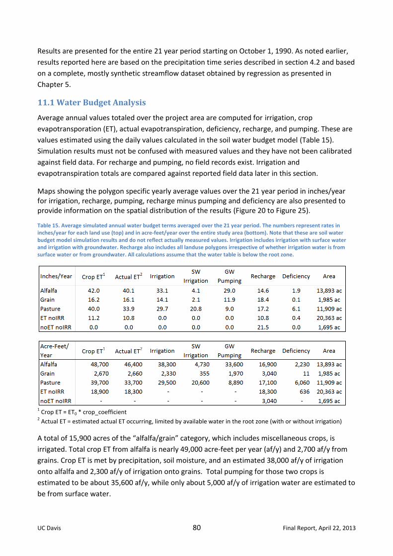
UC Davis 80 Final Report, April 22, 2013
Results are presented for the entire 21 year period starting on October 1, 1990. As noted earlier,
results reported here are based on the precipitation time series described in section 4.2 and based
on a complete, mostly synthetic streamflow dataset obtained by regression as presented in
Chapter 5.
11.1 Water Budget Analysis
Average annual values totaled over the project area are computed for irrigation, crop
evapotransporation (ET), actual evapotranspiration, deficiency, recharge, and pumping. These are
values estimated using the daily values calculated in the soil water budget model (Table 15).
Simulation results must not be confused with measured values and they have not been calibrated
against field data. For recharge and pumping, no field records exist. Irrigation and
evapotranspiration totals are compared against reported field data later in this section.
Maps showing the polygon specific yearly average values over the 21 year period in inches/year for irrigation, recharge, pumping, recharge minus pumping and deficiency are also presented to provide information on the spatial distribution of the results (Figure 20 to Figure 25).
Table 15. Average simulated annual water budget terms averaged over the 21 year period. The numbers represent rates in inches/year for each land use (top) and in acre-feet/year over the entire study area (bottom). Note that these are soil water budget model simulation results and do not reflect actually measured values. Irrigation includes irrigation with surface water and irrigation with groundwater. Recharge also includes all landuse polygons irrespective of whether irrigation water is from surface water or from groundwater. All calculations assume that the water table is below the root zone.
1 Crop ET = ET0 * crop_coefficient
2 Actual ET = estimated actual ET occurring, limited by available water in the root zone (with or without irrigation)
A total of 15,900 acres of the “alfalfa/grain” category, which includes miscellaneous crops, is
irrigated. Total crop ET from alfalfa is nearly 49,000 acre-feet per year (af/y) and 2,700 af/y from
grains. Crop ET is met by precipitation, soil moisture, and an estimated 38,000 af/y of irrigation
onto alfalfa and 2,300 af/y of irrigation onto grains. Total pumping for those two crops is
estimated to be about 35,600 af/y, while only about 5,000 af/y of irrigation water are estimated to
be from surface water.

UC Davis 81 Final Report, April 22, 2013
Irrigated “pasture” including some residential/urban lawn areas covers 12,000 acres with an
estimated total crop ET of nearly 40,000 af/y. Two-thirds of the nearly 30,000 af/y of irrigation
water is from surface water (20,600 af/y) with the remainder from groundwater (8,900 af/y).
Total surface water deliveries to irrigated areas are estimated to be about 26,000 af/y,
groundwater pumping is estimated to be on the order of 44,500 af/y not including groundwater
uptake in about 2,100 acres of subirrigated areas.
An additional 19,000 af/y of consumptive use occurs on lands in the “ET - no Irrigation” land use
areas (including dry farmed or sub-irrigated crops). This estimated ET is supplied by precipitation
and soil moisture storage and does not account for any groundwater uptake.
Analysis of the spatial and temporal distribution of irrigation and recharge fluxes suggests the
following main findings:
Highest irrigation and pumping rates occur in polygons with pasture as land use and
groundwater as water source (Figure 20 and Figure 23): this can be explained by the fact
that pasture has the longest irrigation season. In polygons with groundwater as water
source, irrigation rate and pumping rate are the same.
Highest recharge rates (Figure 21) occur in polygons with pasture as land use and with
groundwater as water source, in vacant land use polygons located in the tailings
subwatershed, and in polygons with very small water holding capacity. Recharge is
expected to be higher where there is higher irrigation or less plant transpiration;
The lowest recharge rates (almost zero recharge) occur, for example, in some polygons
south of Greenview around Highway 3: as shown in Figure 19, they correspond to dryland.
They rely on precipitation as water source for plants, which efficiently scour available
moisture and therefore show little natural recharge, typical of a semi-arid climate;
Low recharge rates (between 4 and 8 in/year) occur in some fields north of Etna: these
have pasture as land use, but they are subirrigated (high water table);
Deficiency (Figure 25) occurs in the months immediately following the end of the irrigation
season (September, October, November).
A year-specific analysis of the water budget for the 21 year period has also been performed
(Figure 26 to Figure 28).This analysis allows us to highlight differences in the water budget
between dry and wet years (highlighted with red and blue arrows, respectively). Dry and wet year
classification is identical to that shown in Figure 6.
As expected, dry years are marked by smaller amounts of recharge to groundwater and a smaller
amount of applied surface water. Lower surface water use reflects the modeled constraints in
irrigation of pasture, which is limited by the estimated or measured (when available) monthly flow
in the stream associated with the subwatersheds to which a field belongs.

UC Davis 82 Final Report, April 22, 2013
Typical characteristics contrasting alfalfa/grain soil water budgets with pasture water budget
dynamics include:
1) Alfalfa/grain land use (Figure 27) is higher in actual evapotranspiration, higher in applied
groundwater and has an overall low fraction of applied surface water. This is expected
considering that alfalfa/grain is mostly groundwater irrigated (Table 14);
2) Pasture land use has higher applied surface water and almost no applied groundwater. The
amount of applied groundwater does not change dramatically from year to year because
there are no large differences in the length of the pasture irrigation season between
different years. Large differences occur in the use of surface water between wet and dry
years. Where the water source is groundwater, year-to-year differences in groundwater
use are small and due to annual differences in the irrigation start date, but then irrigation
continues for the entire season each year, regardless of year type (wet, normal, dry);
3) Recharge in alfalfa/grain is similar to pasture. A few pastures have high recharge rates due
to being irrigated with groundwater at high irrigation rates (low irrigation efficiency
assigned by the model).
Effects of dry and wet years on the amount of applied surface water and applied groundwater are
shown in more detail for alfalfa and for pasture (Figure 29). In dry years, the amount of applied
surface water generally decreases while the amount of groundwater use increases.
The results of the soil water budget model are generally in agreement with what would be
expected considering the background information on land use, irrigation water source, irrigation
type, and precipitation.
The soil water budget model can be adjusted to accommodate changes in inputs and/or
operational assumptions. Further sensitivity analysis and tests can be performed to evaluate
assumptions.
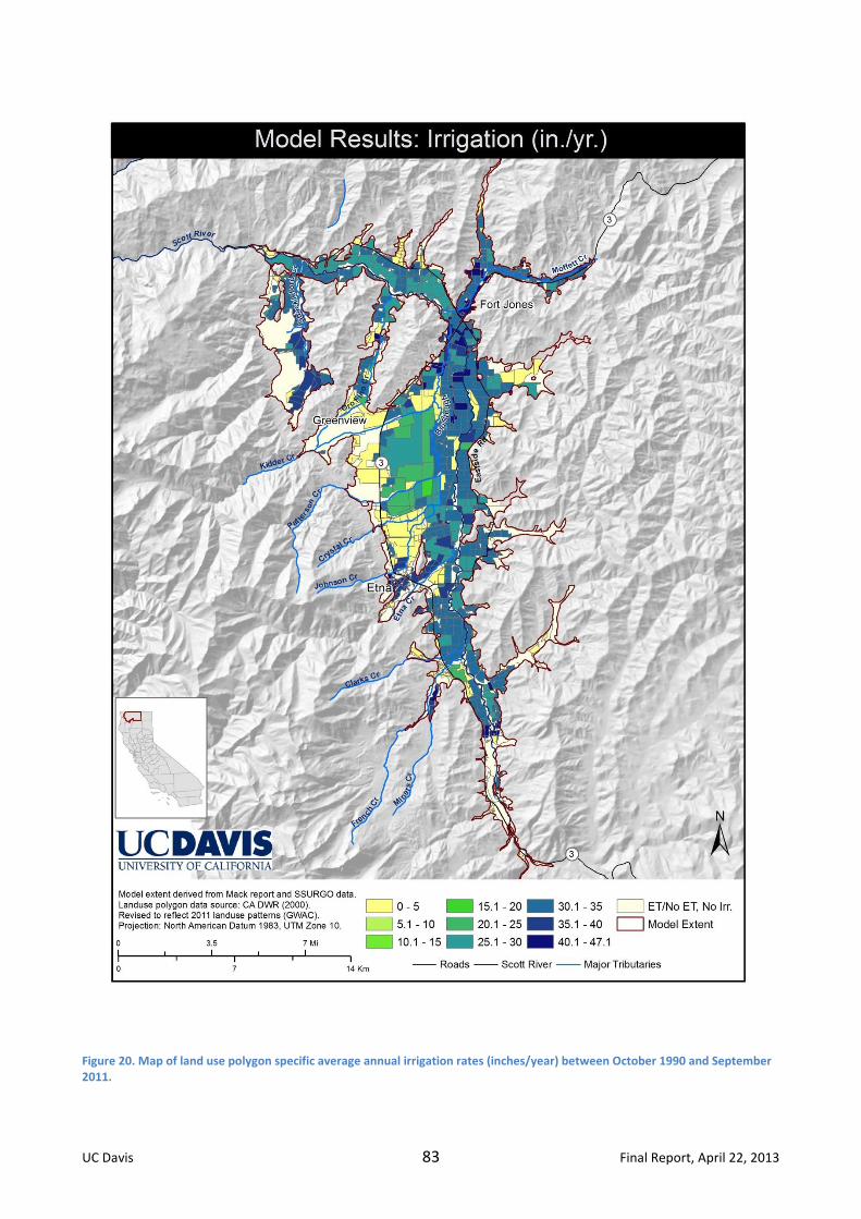
UC Davis 83 Final Report, April 22, 2013
Figure 20. Map of land use polygon specific average annual irrigation rates (inches/year) between October 1990 and September 2011.

UC Davis 84 Final Report, April 22, 2013
Figure 21. Map of land use polygon specific average annual recharge rates (inches/year) between October 1990 and September 2011.

UC Davis 85 Final Report, April 22, 2013
Figure 22. Map of land use polygon specific average annual applied surface water rates (inches/year) between October 1990 and September 2011. The amount of applied surface water is calculated as the difference between the total irrigation and the pumping.

UC Davis 86 Final Report, April 22, 2013
Figure 23. Map of land use polygon specific average annual pumping rates (inches/year) between October 1990 and September 2011.
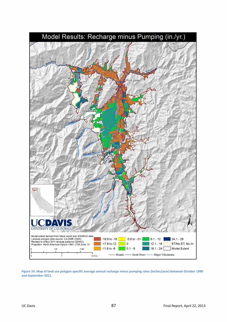
UC Davis 87 Final Report, April 22, 2013
Figure 24. Map of land use polygon specific average annual recharge minus pumping rates (inches/year) between October 1990 and September 2011.

UC Davis 88 Final Report, April 22, 2013
Figure 25. Map of land use polygon specific average annual deficiency rates (inches/year) between October 1990 and September 2011. Deficiency is defined as the difference between actualET and ET under optimal water supply conditions. Deficiency occurs in pasture or after the irrigation season ends in alfalfa

UC Davis 89 Final Report, April 22, 2013
Figure 26. Yearly soil root zone water budget in in/year, area-weighted average for the entire Scott Valley project area. Input to the root zone shown as positive values (precipitation, applied groundwater and surface water). Output from the root zone shown as negative values (actual ET and recharge).
Figure 27. Yearly soil root zone water budget in in/year, area-weighted average for the alfalfa polygons over the entire Scott Valley project area. Input to the root zone shown as positive values (precipitation, applied groundwater and surface water). Output from the root zone shown as negative values (actual ET and recharge).
-80
-60
-40
-20 0
20
40
60
80
1991
1993
1995
1997
1999
2001
2003
2005
2007
2009
2011
Yearly average in in/year
Recharge
ActualET
Precipitation
Applied GroundwaterApplied Surface Water
Wet year: higher recharge
Dry year: little recharge
-70
-60
-50
-40
-30
-20
-10 0
10
20
30
40
50
60
70
1991
1993
1995
1997
1999
2001
2003
2005
2007
2009
2011
Yearly average in in/year
Recharge
ActualET
Precipitation
Applied GroundwaterApplied Surface Water

UC Davis 90 Final Report, April 22, 2013
Figure 28 Yearly soil root zone water budget in in/year, area-weighted average for the pasture polygons over the entire Scott Valley project area. Input to the root zone shown as positive values (precipitation, applied groundwater and surface water). Output from the root zone shown as negative values (actual ET and recharge).
-70
-60
-50
-40
-30
-20
-10 0
10
20
30
40
50
60
70
1991
1993
1995
1997
1999
2001
2003
2005
2007
2009
2011
Yearly average in in/year
Recharge
ActualET
Precipitation
Applied GroundwaterApplied Surface Water

UC Davis 91 Final Report, April 22, 2013
Figure 29. Yearly values of applied surface water and applied groundwater in in/year for alfalfa/grain (above) and pasture (below), area-weighted average over all alfalfa/grain land use polygons in the project area. Dry years are highlighted.
11.2 Sensitivity Analysis: Water Holding Capacity
Water holding capacity is a critical parameter in the soil water budget model. But the actual value
of the parameter is quite variable and locally uncertain. Based on expert suggestions, to compute
the above results we used a water holding capacity that corresponds to a rooting depth of 4 feet. Roots
may eventually grow deeper than 4 feet and access deeper water if shallow moisture is depleted.
0
5
10
15
20
25
30
35
40
45
1 2 3 4 5 6 7 8 9 10 11 12 13 14 15 16 17 18 19 20 21
Applied Groundwater Applied Restricted Surface Water
Alfalfa
0
5
10
15
20
25
30
35
40
45
1 2 3 4 5 6 7 8 9 10 11 12 13 14 15 16 17 18 19 20 21
Pasture
in/year
Water year 1991-2011
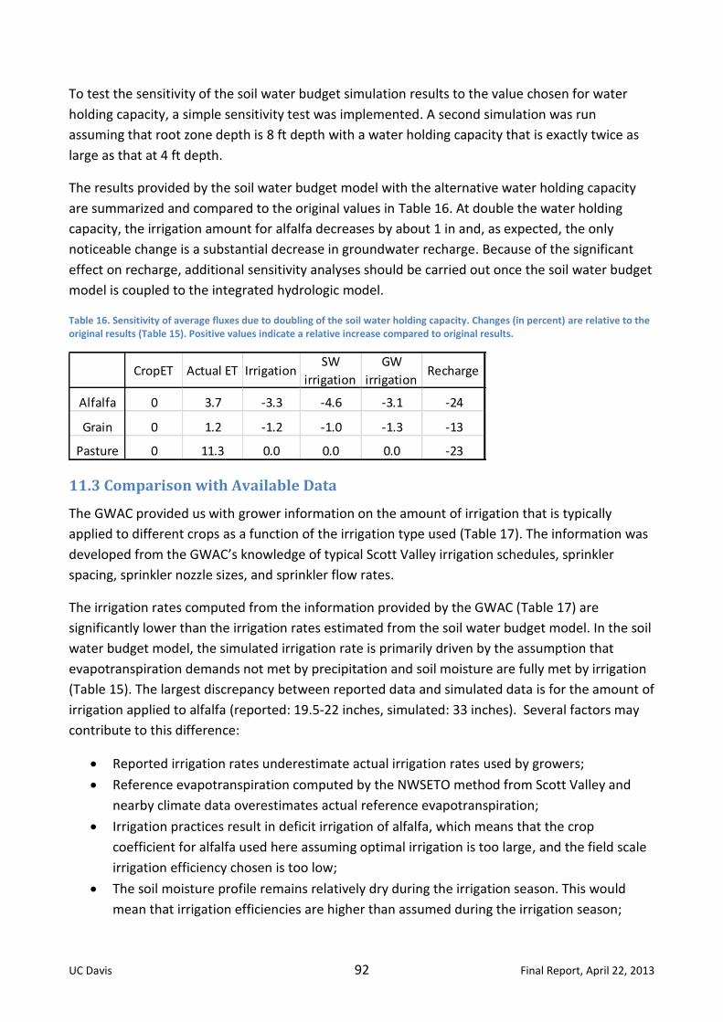
UC Davis 92 Final Report, April 22, 2013
To test the sensitivity of the soil water budget simulation results to the value chosen for water
holding capacity, a simple sensitivity test was implemented. A second simulation was run
assuming that root zone depth is 8 ft depth with a water holding capacity that is exactly twice as
large as that at 4 ft depth.
The results provided by the soil water budget model with the alternative water holding capacity
are summarized and compared to the original values in Table 16. At double the water holding
capacity, the irrigation amount for alfalfa decreases by about 1 in and, as expected, the only
noticeable change is a substantial decrease in groundwater recharge. Because of the significant
effect on recharge, additional sensitivity analyses should be carried out once the soil water budget
model is coupled to the integrated hydrologic model.
Table 16. Sensitivity of average fluxes due to doubling of the soil water holding capacity. Changes (in percent) are relative to the original results (Table 15). Positive values indicate a relative increase compared to original results.
11.3 Comparison with Available Data
The GWAC provided us with grower information on the amount of irrigation that is typically
applied to different crops as a function of the irrigation type used (Table 17). The information was
developed from the GWAC’s knowledge of typical Scott Valley irrigation schedules, sprinkler
spacing, sprinkler nozzle sizes, and sprinkler flow rates.
The irrigation rates computed from the information provided by the GWAC (Table 17) are
significantly lower than the irrigation rates estimated from the soil water budget model. In the soil
water budget model, the simulated irrigation rate is primarily driven by the assumption that
evapotranspiration demands not met by precipitation and soil moisture are fully met by irrigation
(Table 15). The largest discrepancy between reported data and simulated data is for the amount of
irrigation applied to alfalfa (reported: 19.5-22 inches, simulated: 33 inches). Several factors may
contribute to this difference:
Reported irrigation rates underestimate actual irrigation rates used by growers;
Reference evapotranspiration computed by the NWSETO method from Scott Valley and
nearby climate data overestimates actual reference evapotranspiration;
Irrigation practices result in deficit irrigation of alfalfa, which means that the crop
coefficient for alfalfa used here assuming optimal irrigation is too large, and the field scale
irrigation efficiency chosen is too low;
The soil moisture profile remains relatively dry during the irrigation season. This would
mean that irrigation efficiencies are higher than assumed during the irrigation season;
CropET Actual ET IrrigationSW
irrigation
GW
irrigationRecharge
Alfalfa 0 3.7 -3.3 -4.6 -3.1 -24
Grain 0 1.2 -1.2 -1.0 -1.3 -13
Pasture 0 11.3 0.0 0.0 0.0 -23

UC Davis 93 Final Report, April 22, 2013
The root zone depth is much larger than 4 feet and roots may possibly tap into the water
table;
A combination of the above.
To address this discrepancy, field experiments were developed in spring of 2012 to collect more
information on alfalfa evapotranspiration, reference evapotranspiration, irrigation rates, soil
moisture dynamics, groundwater levels, and forage yield. Eight alfalfa fields (four center pivot
irrigated and four wheel-line sprinkler irrigated fields) were selected for monitoring over the 2012-
2013 production season. Data collected include:
1. Three surface renewal system installed in three alfalfa fields (all of the irrigated with center pivots that have permanently installed flow meters) to calculate alfalfa ET.
2. A CIMIS type weather station installed in one irrigated pasture field to estimate ETo in order to determine the appropriate alfalfa crop coefficient.
3. Soil samples collected to 8 ft. depth in April, August, and early October to determine gravimetric soil moisture content.
4. Watermark soil moisture sensors installed at 1 ft. increments to 8 ft. depth at two locations in all fields to determine soil moisture tension and wetting and drying patterns over the season.
5. A tipping rain gauge installed in each field to monitor irrigation application rate and in-season rainfall.
6. Portable Ultrasonic Doppler flow meter used to determine flow rate in center pivot fields. 7. Nozzle discharge rate monitored in wheel-line fields. 8. Alfalfa yield determined in all eight fields by hand cutting a representative area and
comparing with grower yield values. The project is intended to be continued for at least one, possibly two years, depending on
interannual variability in the dataset. The dataset will be critical to help refine the soil water
budget model to minimize the difference between simulated and measured irrigation rates.
Table 17. Total seasonal irrigation amount computed from information on typical irrigation frequency, nozzle sizes, nozzle spacing, and nozzle flow rates, provided by the GWAC for each crop and each irrigation type.
Alfalfa Grain Pasture
Irrigation Type
Irrigation in inches Irrigation
Type Irrigation in
inches Irrigation
Type Irrigation in
inches
Sprinkler 22” Sprinkler 8.25” Sprinkler n/a
Center Pivot 19.5” Center Pivot 6” Center Pivot n/a

UC Davis 94 Final Report, April 22, 2013
12 Future Work
Work that is currently planned or ongoing will concentrate on four main tasks: 1) evaluation of the
field experiments to determine alfalfa irrigation and evapotranspiration rates, 2) refinement of
the soil water budget model, 3) development of Version 2 of the Scott Valley Integrated
Hydrologic Model, and 4) initiation of scenario alternatives to simulate future streamflow and
groundwater conditions under various management/project options.
The dataset produced with the effort presented in this report is used to build Version 2 of the
Scott Valley Integrated Hydrologic Model. The model is implemented using MODFLOW-2000 and it
will be coupled to the soil water budget model and streamflow data presented here. The soil
water budget model provides groundwater pumping, surface water diversion, and groundwater
recharge rates that are also used as inputs in the groundwater flow model. It also provides the
evapotranspiration data for the water budget.
In summary, Version 2 of the Scott Valley Integrated Hydrologic Model will perform the following
refinements that are improvements over the (draft) Version 1 of the model:
1. Extended modeling area to include the dredge-tailing area in the southern Scott Valley and
make some minor adjustments to the edge of the modeling area, based primarily on land
surface topography data.
2. Refined land surface elevation representation, especially of stream channels, using neìwly
available LIDAR data obtained from the U.S. Forest Service.
3. Updated groundwater pumping, surface water diversion, and groundwater recharge using
the values calculated with the new soil water budget model.
4. Revised regression model of streamflow data based on the evaluation of additional data
that have become available since 2008.
5. Extension of the time period simulated by the integrated hydrologic model to include 2009,
2010, and most of 2011 (through September 30, 2011).
6. Extensive sensitivity analysis, calibration and uncertainty analysis.
Regarding this last task, parameters from both models (the soil water budget model and the
MODFLOW integrated hydrologic model) will be included simultaneously in the sensitivity analysis
allowing us to evaluate the sensitivity of model results to parameters and observations. The
integrated hydrologic model will be calibrated and validated using measured groundwater level
data available for the Scott Valley and using measured streamflow data downstream of Scott
Valley.
The information that we obtain with this type of analysis will quantify and illustrate the sensitivity
of model results to parameters and algorithm choice. It will also describe the relationship between
different types of data and the processes represented. Furthermore, our approach will allow the
evaluation of uncertainty in the model output for 1991-2011 and for any of the scenario analyses.
The sensitivity analysis will be used to identify the most critical information needed to reduce
model prediction uncertainty. The evaluation of data needs will include a determination of optimal

UC Davis 95 Final Report, April 22, 2013
areas or locations at which to collect data and whether there are seasonal preferences to
collecting certain data. All these tasks will be performed using an automatic inversion code such as
UCODE_2005 (Poeter et al., 2005) or PEST (Doherty, 2010) which allow the coupling of the two
models and the automatic calibration of parameters involved in all the processes.
The approach described in this report and the integrated hydrologic model currently under
development provide a framework to efficiently and effectively develop and evaluate future data
collection campaigns and alternative water management scenarios. In the soil water budget model
much of the information related to a field is parameterized with parameters available from
geospatial databases. Future water management scenarios can be efficiently coded into the soil
water budget model and the integrated hydrologic model as needed to simulate future conditions.
UC Davis 96 Final Report, April 22, 2013
13 Conclusions
Precipitation and streamflow data have been analyzed, a revised streamflow regression model to
generated synthetic data for stations that have only a very limited period of record has been
prepared specifically for use with the integrated hydrologic model, and a new conceptual model
for the simulation of the soil water budget has been developed and used to estimate streamflow
diversions, groundwater pumping, groundwater recharge, and crop evapotranspiration. The model
is based on a spatially distributed soil water dynamics approach and puts together a wide array of
information in a tractable, physically and hydrologically rigorous approach.
Comprehensive datasets were compiled, and we worked closely with local stakeholders and
committees to refine these dataset as well as the conceptual framework used to represent various
landuses, especially agricultural landuses, and irrigation management practices. The contributions
of various stakeholders have been essential to update our GIS database and soil water budget
model with the most complete, accurate reflection of land use and agricultural practices in Scott
Valley.
The study shows that precipitation across the valley floor, while variable during any given rainfall
event, is overall of similar magnitude between Callahan, Fort Jones, and Greenview. Significantly
higher precipitation may occur at the far western margin of the valley (Etna), but available data do
not allow for sufficient quantification of such effects. Precipitation patterns define streamflow.
Years with low precipitation result in the lowest summer flows on the Scott River and its
tributaries. We are able to estimate tributary flows with a newly developed statistical model that
takes advantage of the long time series at the Ft. Jones streamflow gauging station immediately
downstream from Scott Valley. The statistical model also shows that snow pack and precipitation
data further aid in tributary streamflow estimation, even if only slightly. Also, developing separate
regression models for the time period before fall of 1972 and the period since then, further
improves statistical estimates of tributary streamflow into the Scott Valley. However, the data
series for the tributaries are extremely limited. The synthetic dataset generated will be sufficient
for purposes of the integrated hydrologic model. It will be important to continue streamflow
monitoring on all tributaries.
Landuse in the Scott Valley, for hydrologic purposes, can be divided into four categories: irrigated
fields in alfalfa-grain rotation (nearly 16,000 acres), irrigated fields with pasture (12,000 acres),
non-irrigated parcels with natural or other vegetation that consumes water through
evapotranspiration, and land parcels that are effectively barren of vegetation or open water
bodies (no irrigation and no evapotranspiration).
Soil water budget simulations show that significant amount of groundwater recharge occurs
across the Scott Valley from both precipitation and irrigation. We estimate that the average
annual recharge is 15 inches in alfalfa, and about 17-18 inches in grain and pasture. Irrigation on
alfalfa is highest (33 inches), followed by pasture (30 inches) and grain (14 inches), which has a
relatively short growing season. Based on soil water budget simulations, groundwater pumping is
estimated to be highest in alfalfa fields, averaging 29 inches per year, supplying most of the

UC Davis 97 Final Report, April 22, 2013
irrigation water there. It is much lower in grain fields (less than 12 inches per year), and lowest in
pasture (averaging 9 inches per year), since most pasture is irrigated with surface water. Rainfall
also provides a significant amount of crop water supplies via soil moisture storage.
Large field-to-field and year-to-year variations occur both with groundwater pumping and
recharge. The variability shown in this report is due to varying irrigation practices within the same
crop type, varying water sources, and due to inter-annual climate variations. Variability within
fields or between individual growers is not simulated, but further adds to actual variability in
groundwater use and recharge.
The alfalfa irrigation results obtained with the simulation model are much higher than recently
measured and grower-reported irrigation rates, thus clearly identifying the need for further
research work to clarify actual irrigation practices and to measure evapotranspiration occurring in
alfalfa fields. Work is needed to test to what degree the discrepancy between measured and
simulated irrigation rates is due to soil moisture storage currently not accounted for, potential
water table encroachment and root water uptake directly from groundwater, variability in actual
irrigation rates, or possibly misleading ET rates published by the California Department of Water
Resources and available in the scientific literature. It will be important to thoroughly validate and
possibly improve the soil water budget model against new field data as part of performing water
management scenario simulations and prior to making policy decisions.
Finally, we recognize that a tool such as the one presented here is critical for discussion of
alternative water management scenarios with the Groundwater Advisory Committee and other
stakeholders as an effective mechanism to mitigate conflicts.
UC Davis 98 Final Report, April 22, 2013
14 References
Allen, R.G., Pereira, L.S., Raes, D., and Smith, M., 1998, Crop evapotranspiration-Guidelines for computing water requirements-FAO Irrigation and drainage paper 56. Food and Agriculture Organization of the United Nations, Rome, Italy: FAO.
California Department of Water Resources. 1963, Land and Water Use in Shasta-Scott Valleys Hydrographic Unit. Volume I: Text, Bulletin No. 94-5, pp. 232.
California Department of Water Resources, 2000, Land Use Survey, Siskiyou County. Available online at http://www.water.ca.gov/landwateruse/lusrvymain.cfm. Accessed May 14, 2009.
Carle, S., and Fogg, G., 1996, Modeling Spatial Variability with One and Multidimensional Continuous-Lag Markov Chains Mathematical Geology Volume 29, Number 7, 891-918, DOI: 10.1023/A:1022303706942.
Deas, M.L., and S.K. Tanaka, 2003, Scott River Water Balance Study: Data Analysis and Model Review. Prepared for the Scott River Watershed Council.
Deas, M.L., and S.K. Tanaka, 2004, Scott River Water Balance Study: Data Analysis and Model Review, Watercourse Engineering, June 2004.
Deas, M.L., and S.K. Tanaka, 2005, Scott River Runoff Forecast Model: Investigation of Potential Formulation, Watercourse Engineering, December 2005.
Deas, M.L., and S.K. Tanaka, 2006, Scott River Water Supply Indices: Year Types for the Scott River Basin, prepared for the Siskiyou RCD.
Deas, M.L., and S.K. Tanaka, 2008, Scott River Water Balance-Streamflow and Precipitation Gauging, prepared for the Siskiyou RCD.
Doherty, J., 2010, Methodologies and Software for PEST-Based Model Predictive Uncertainty Analysis, Watermark Numerical Computing, Australia.
Drake, D., Tate, K., and Carlson, H., 2000, Analysis shows climate-caused decreases in Scott River Fall Flows, California Agriculture, Vol. 54 n. 6, pp. 46-49.
Foglia, L., A. McNally, L. Ledesma, R. Hines, and T. Harter, 2012, Scott Valley Integrated Hydrologic Model: Background and Water Budget (Draft Report). Prepared for the North Coast RWQCB.
Gesch, D.B., 2007, The National Elevation Dataset, in Maune, D., ed., Digital Elevation Model Technologies and Applications: The DEM Users Manual, 2nd Edition: Bethesda, Maryland, American Society for Photogrammetry and Remote Sensing, p. 99-118.
Gesch, D., et al., 2002, The National Elevation Dataset: Photogrammetric Engineering and Remote Sensing, v. 68, no. 1, p. 5-11.
Hanson, B., Orloff, S., Bali, K., Sanden, B., Putnam, D., 2011a, Evapotranspiration of Fully-Irrigated Alfalfa in Commercial Fields, 2011 Conference Proceedings, Agricultural Certification Programs-Opportunities and Challenges.

UC Davis 99 Final Report, April 22, 2013
Hanson, B., Orloff, S., Bali, K., Sanden, B., Putnam, D., 2011b, Mid-summer Deficit Irrigation of Alfalfa in Commercial Fields, 2011 Conference Proceedings, Agricultural Certification Programs-Opportunities and Challenges.
Harbaugh, A.W., Banta, E.R., Hill, M.C. and McDonald, M.G., 2000, MODFLOW-2000, The U.S. Geological Survey modular ground-water model – users guide to modularization concepts and the ground-water flow process: U.S. Geological Survey Open-File Report 00-92, 121 p.
Hargreaves, G. H., and Z. A. Samani, 1982, Estimating potential evapotranspiration, J. Irrig. Drain. Eng., 108(3), 225-230.
Hargreaves, G.H., and J.P. Riley, 1985, Irrigation water requirements for the Senegal river basin. Journal of Irrigation and Drainage Engineering 111(3): 265-275.
Harter, T., and R. Hines, 2008, Scott Valley Community Groundwater Study Plan. Groundwater Cooperative Extension Program, University of California, Davis.
Hines, Ryan. “MS Thesis Draft.” October 2010.
Mack, S., 1958, Geology and Ground-Water Features of Scott Valley Siskiyou County, California: U.S. Geological Survey Water-Supply Paper 1462. Washington D.C.
Monteith, J.L. , 1965, Evaporation and environment. Symp. Soc. Exp. Biol. 19, 205-224.
North Coast Regional Water Quality Control Board, 2006, Action Plan for the Scott River Sediment and Temperature Total Maximum Daily Loads, September 2006.
North Coast Regional Water Quality Control Board, Staff report for the action plan for the Scott River Watershed Sediments and Temperature TMDLs, 2011, http://www.swrcb.ca.gov/northcoast/water_issues/programs/tmdls/scott_river/staff_report.shtml.
Orang, M.N., Snyder, R.L., Matyac, J.S., 2008, Consumptive Use Program +, California Department of Water Resources, http://www.water.ca.gov/landwateruse/models.cfm.
Poeter, E.P., Hill, M.C., Banta, E.R., Mehl, S.W., and Christensen, S., 2005, UCODE-2005 and six other computer codes for universal sensitivity analysis, inverse modeling, and uncertainty evaluation, U.S. Geological Survey Techniques and Methods, 6-A11.
Quigley, D., S. Farber, K. Conner, J. Power, and L. Bundy, 2001, Water Temperatures in the Scott River Watershed in Northern California.” Prepared for U.S. Fish and Wildlife Service.
Snyder, R.L., M. Orang and S. Matyac, 2002, A long-term water use planning model for California. Proceedings of the Sixth International Symposium on Computer Modelling in Fruit Research and Orchard Management. Acta Hort., 584: 115-121.
Soil Survey Staff, Natural Resources Conservation Service, United States Department of Agriculture, 1975, Soil Survey Geographic (SSURGO) Database for [Survey Area, State]. Available online athttp://soildatamart.nrcs.usda.gov . State of California, State Water Resources Control Board, 1975.
S.S. Papadopulos & Associates, 2012, Groundwater conditions in Scott Valley, Report prepared for the Karuk Tribe, March 2012.

UC Davis 100 Final Report, April 22, 2013
Swenson, M. 1947. Report on Scott River Watershed Basic Data Pertinent to Development of a Watershed Management Plan for the Klamath National Forest. Region 5. U.S. Forest Service.
Tanaka, S.K., and M.L. Deas, 2008, Scott River Water Balance: Streamflow and Precipitation Gauging.” Watercourse Engineering, May 2008.
UCCE Leaflet 21427, Using Reference Evapotranspiration (ET0) and Crop Coefficients to estimate Crop Evapotranspiration (Etc) for agronomic crops, grasses, and vegetable crops, http://lawr.ucdavis.edu/irrigation/irrigation_leaflets/L21427.html
Van Kirk, R. W. and S. W. Naman, 2008, Relative Effects of Climate and Water Use on Base-Flow Trends in the Lower Klamath Basin. Journal of the American Water Resources Association (JAWRA) 44(4):1035-1052. DOI: 10.1111/j.1752-1688.2008.00212.x
Watershed Sciences, 2010, LiDAR Remote Sensing Data Collection: Scott Valley California. November 11, 2010. Watershed Sciences, 529 SW 3rd Avenue, Suite 300, Portland, OR 97204. 24 pages. Accessed through the California State Water Resources Control Board.
Streamflow - Data Sources
California Rivers Assessment (CARA). “Historic Precipitation for Scott Basin.” Information Center for the Environment, University of California, Davis. January 1998. http://www.ice.ucdavis.edu/newcara/basin.asp?cara_id=15 (retrieved on 28 June 2012)
California Data Exchange Center (CDEC). “Historical Data for Scott River Basin.” California Department of Water Resources. 2010. http://cdec.water.ca.gov/ (retrieved on 28 June 2012).
National Oceanic and Atmospheric Administration (NOAA). “Climate Data Online Data Search: Scott Valley.” http://www.ncdc.noaa.gov/cdo-web/ (retrieved on 29 June 2012).
USGS Water Data for the Nation. “USGS Surface-Water Daily Data for the Nation.” http://waterdata.usgs.gov/ (retrieved on 23 August 2012).
California Department of Water Resources. “Water Data Library.” http://www.water.ca.gov/waterdatalibrary/ (retrieved on 23 July 2012)
Streamflow - Statistical Analysis Software
AnalystSoft Inc. StatPlus®: mac LE. 2011. http://www.analystsoft.com/en/products/statplusmacle/
R Core Team. R: A language and environment for statistical computing. R Foundation for Statistical Computing. Vienna, 2012. http://www.R-project.org

UC Davis 101 Final Report, April 22, 2013
15 Appendix A
The appendix illustrates detailed results of the streamflow regression analysis (Section 5). Due to
its size, this appendix is provided as a separate PDF file.