arX

iv:1

311.

3342

v2 [

hep-

ph]

28

Jan

2014

ZU-TH 26/13November 2013

Schouten identities for Feynman graph amplitudes;

the Master Integrals for the two-loop massive sunrise graph

Ettore Remiddia, 1 and Lorenzo Tancredib, 2

a Dipartimento di Fisica, Universita di Bologna and INFN, Sezione di Bologna, I-40126 Bologna, Italy

b Institut fur Theoretische Physik, Universitat Zurich, Wintherturerstrasse 190, CH-8057 Zurich,

Switzerland

Abstract

A new class of identities for Feynman graph amplitudes, dubbed Schouten identities, valid at fixedinteger value of the dimension d is proposed. The identities are then used in the case of the two-loopsunrise graph with arbitrary masses for recovering the second-order differential equation for the scalaramplitude in d = 2 dimensions, as well as a chained set of equations for all the coefficients of theexpansions in (d− 2). The shift from d ≈ 2 to d ≈ 4 dimensions is then discussed.

Key words: Feynman graphs, Multi-loop calculations, Schouten identities

1e-mail: ettore.remiddi@bo.infn.it2e-mail: tancredi@physik.uzh.ch

1 Introduction

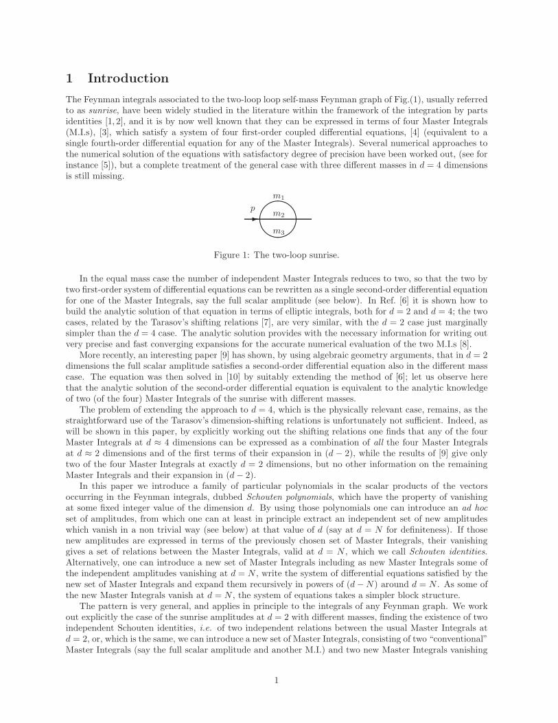
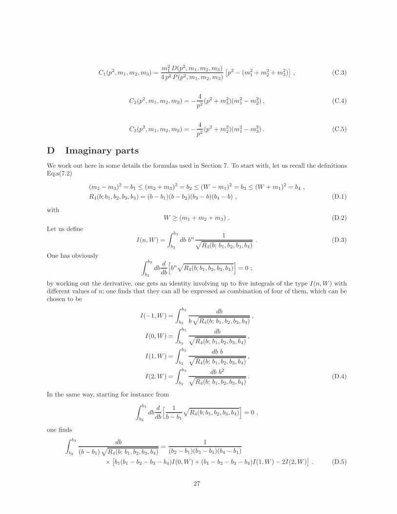
The Feynman integrals associated to the two-loop loop self-mass Feynman graph of Fig.(1), usually referredto as sunrise, have been widely studied in the literature within the framework of the integration by partsidentities [1, 2], and it is by now well known that they can be expressed in terms of four Master Integrals(M.I.s), [3], which satisfy a system of four first-order coupled differential equations, [4] (equivalent to asingle fourth-order differential equation for any of the Master Integrals). Several numerical approaches tothe numerical solution of the equations with satisfactory degree of precision have been worked out, (see forinstance [5]), but a complete treatment of the general case with three different masses in d = 4 dimensionsis still missing.

✲✫✪✬✩m1

m2

m3

p

Figure 1: The two-loop sunrise.

In the equal mass case the number of independent Master Integrals reduces to two, so that the two bytwo first-order system of differential equations can be rewritten as a single second-order differential equationfor one of the Master Integrals, say the full scalar amplitude (see below). In Ref. [6] it is shown how tobuild the analytic solution of that equation in terms of elliptic integrals, both for d = 2 and d = 4; the twocases, related by the Tarasov’s shifting relations [7], are very similar, with the d = 2 case just marginallysimpler than the d = 4 case. The analytic solution provides with the necessary information for writing outvery precise and fast converging expansions for the accurate numerical evaluation of the two M.I.s [8].

More recently, an interesting paper [9] has shown, by using algebraic geometry arguments, that in d = 2dimensions the full scalar amplitude satisfies a second-order differential equation also in the different masscase. The equation was then solved in [10] by suitably extending the method of [6]; let us observe herethat the analytic solution of the second-order differential equation is equivalent to the analytic knowledgeof two (of the four) Master Integrals of the sunrise with different masses.

The problem of extending the approach to d = 4, which is the physically relevant case, remains, as thestraightforward use of the Tarasov’s dimension-shifting relations is unfortunately not sufficient. Indeed, aswill be shown in this paper, by explicitly working out the shifting relations one finds that any of the fourMaster Integrals at d ≈ 4 dimensions can be expressed as a combination of all the four Master Integralsat d ≈ 2 dimensions and of the first terms of their expansion in (d − 2), while the results of [9] give onlytwo of the four Master Integrals at exactly d = 2 dimensions, but no other information on the remainingMaster Integrals and their expansion in (d− 2).

In this paper we introduce a family of particular polynomials in the scalar products of the vectorsoccurring in the Feynman integrals, dubbed Schouten polynomials, which have the property of vanishingat some fixed integer value of the dimension d. By using those polynomials one can introduce an ad hoc

set of amplitudes, from which one can at least in principle extract an independent set of new amplitudeswhich vanish in a non trivial way (see below) at that value of d (say at d = N for definiteness). If thosenew amplitudes are expressed in terms of the previously chosen set of Master Integrals, their vanishinggives a set of relations between the Master Integrals, valid at d = N , which we call Schouten identities.Alternatively, one can introduce a new set of Master Integrals including as new Master Integrals some ofthe independent amplitudes vanishing at d = N , write the system of differential equations satisfied by thenew set of Master Integrals and expand them recursively in powers of (d−N) around d = N . As some ofthe new Master Integrals vanish at d = N , the system of equations takes a simpler block structure.

The pattern is very general, and applies in principle to the integrals of any Feynman graph. We workout explicitly the case of the sunrise amplitudes at d = 2 with different masses, finding the existence of twoindependent Schouten identities, i.e. of two independent relations between the usual Master Integrals atd = 2, or, which is the same, we can introduce a new set of Master Integrals, consisting of two “conventional”Master Integrals (say the full scalar amplitude and another M.I.) and two new Master Integrals vanishing

1

at d = 2. The system of differential equations satisfied by the new set of Master Integrals can then beexpanded in powers of (d − 2). At zeroth-order we find a two by two system for the two “conventional”M.I.s (the other two Master Integrals vanish), equivalent to the second-order equation found in [9], whileat first-order in (d − 2) we find in particular two relatively simple equations for the first terms of theexpansion of the two new M.I.s, in which the zeroth-orders of the two “conventional” M.I.s appear as nonhomogeneous known terms.

One can move from d ≈ 2 to the physically more interesting d ≈ 4 case by means of the Tarasov’sshifting relations; it is found that for obtaining the zeroth-order term in (d− 4) of all the four M.I.s (of theold or of the new set) at d ≈ 4 one needs, besides the zeroth-order term in (d − 2) of the two “old” M.I.sat d ≈ 2, also the first term in (d− 2) of the new M.I.s.

The plan of the paper is as follows: in sec. 2 we introduce the Schouten polynomials for an arbitrarynumber of dimensions, while their applications to Feynman Amplitudes is discussed in sec. 3. In sec. 4 weshow how, by using the Schouten Identities, a new set of Master Integrals can be found, whose differentialequations in d = 2 take an easier block form and can be therefore re-casted (see sec. 5) as a second-orderdifferential equation for one of the Masters. In sec. 6 we show how the results at d ≈ 4 can be recovered fromthose at d ≈ 2 through Tarasov’s shifting relations. Finally, in sec. 7, which is somewhat pedagogical, wepresent a thorough treatment of the imaginary parts of the Master Integrals in d = 2 and d = 4 dimensions.Many lengthy formulas and some explicit derivations can be found in the Appendices at the end of thepaper.

2 The Schouten Polynomials

As an introduction, let us recall that in d = 4 dimensions one cannot have more than 4 linearly independentvectors; indeed, given five vectors vα, aµ, bν , cρ, dσ in four dimensions they are found to satisfy the followingrelation

vµǫ(a, b, c, d)− aµǫ(v, b, c, d)− bµǫ(a, v, c, d)− cµǫ(a, b, v, d)− dµǫ(a, b, c, v) = 0 , (2.1)

where ǫµνρσ is the usual Levi-Civita tensor with four indices, with ǫ1234 = 1, etc., and following the con-vention introduced in the program SCHOONSCHIP [11] we use

ǫ(a, b, c, d) = ǫµνρσaµbνcρdσ . (2.2)

Eq.(2.1) is known as the Schouten identity [12]; by squaring it, one gets a huge polynomial, of fifth-order inthe scalar products of all the vectors. Due to Eq.(2.1), that polynomial vanishes in d = 4 dimensions (and,a fortiori for any integer dimension d ≤ 4); note however that the polynomial does not vanish identicallyfor any arbitrary value of the dimension; as Eq.(2.1) is valid only when d ≤ 4, for d > 4 the polynomial isnot bound to take a vanishing value.

As an extension (or rather a simplification) of Eq.(2.1), consider now the quantity

ǫ(a, b) = ǫµνaµbν , (2.3)

where ǫµν is the Levi-Civita tensor with two indices (defined of course by ǫ12 = −ǫ21 = 1, ǫ11 = ǫ22 = 0),and aµ, bν are a couple of two-dimensional vectors. By squaring it, Eq.(2.3) gives at once

ǫ2(a, b) = a2b2 − (a · b)2 , (2.4)

where a2, b2 are the squared moduli of the vectors aµ, bν and (a · b) their scalar product.So far, all the quantities introduced in Eq.s(2.3,2.4) are in d = 2 dimensions. If the dimension d takes thevalue of any (non-vanishing) integer less than 2 (i.e. if d = 1), the r.h.s. of Eq.(2.3) vanishes, and so doesthe r.h.s. of Eq.(2.4) as well. At this point we define the Schouten Polynomial P2(d; a, b) as

P2(d; a, b) = a2b2 − (a · b)2 , (2.5)

where the r.h.s. is formally the same r.h.s. of Eq.(2.4), but the two vectors aµ, bν are assumed to be d-dimensional vectors, with continuous d. To emphasize that point, we have written d within the arguments

2

of the Schouten Polynomial, even if d does not appear explicitly in the r.h.s. of Eq.(2.5). By the verydefinition, at integer non vanishing dimension d < 2 (i.e. at d = 1), P2(d; a, b) vanishes,

P2(1; a, b) = 0 , (2.6)

as can be also verified by an absolutely trivial explicit calculation.Following the elementary procedure leading to Eq.(2.5), given in d = 3 dimensions any triplet of vectors

aµ, bν , cρ we considerǫ(a, b, c) = ǫµνρaµbνcρ , (2.7)

where ǫµνρ is the Levi-Civita tensor with three indices (defined as usual by ǫ123 = 1 etc.) and then weevaluate its square

ǫ2(a, b, c) = a2b2c2 − a2(b · c)2 − b2(a · c)2 − c2(a · b)2 + 2(a · b)(b · c)(a · c) . (2.8)

We then define the Schouten Polynomial P3(d; a, b, c) as

P3(d; a, b, c) = a2b2c2 − a2(b · c)2 − b2(a · c)2 − c2(a · b)2 + 2(a · b)(b · c)(a · c) . (2.9)

where again the r.h.s. is formally the same as in Eq.(2.8), but the three vectors aµ, bν , cρ are assumed tobe d-dimensional vectors, with continuous d. By construction, P3(d; a, b, c) vanishes at d = 1 and at d = 2,

P3(1; a, b, c) = 0 ,

P3(2; a, b, c) = 0 . (2.10)

Needless to say, the procedure can be immediately iterated to any higher dimension, generating Schoutenpolynomials involving four vectors and vanishing in d = 1, 2, 3 dimensions, or involving five vectors andvanishing in d = 1, 2, 3, 4 dimensions, corresponding, up to a constant numerical factor, to the square ofEq.(2.1), etc..

As it is apparent from the previous discussion, the Schouten polynomials generated by a given set ofvectors are nothing but the Gram determinants of the corresponding vectors; we prefer to refer to them asSchouten polynomials to emphasize that they vanish in any integer dimension d less than the number ofthe vectors.

In the actual physical applications, as one is interested mainly in the d → 4 limit of Feynman graphamplitudes, one can reach d = 4 starting from a different value of d and then moving to d = 4 by meansof the Tarasov’s shifting relations [7]. As the shift relates values of d differing by two units, the d = 1Schouten identities, easily established for any amplitude in which at least two vectors occur, are of no use.The next simplest identities are at d = 2 and occur with any amplitude involving at least three vectors.That is the case of the two-loop self-mass graph (the sunrise), which we will study in this paper in thearbitrary mass case.

3 The Schouten Identities for the Sunrise graph

We discuss in this Section the use of the Schouten polynomial P3(d; a, b, c) in the case of the sunrise, thetwo-loop self-mass graph of Fig.(1).

The external momentum is p and the internal masses are m1,m2,m3. We use the Euclidean metric, sothat p2 is positive when spacelike; sometimes we will use also s = W 2 = −p2, so that the sunrise amplitudesdevelop an imaginary part when

√s = W > (m1 + m2 +m3), the threshold of the Feynman graph. We

write the propagators as

D1 = q21 +m21 ,

D2 = q22 +m22 ,

D3 = (p− q1 − q2)2 +m2

3 , (3.1)

3

and define the loop integration measure, in agreement with previous works, as:

∫

Ddq =

1

C(d)

∫

ddq

(2π)d−2, (3.2)

with

C(d) = (4π)(4−d)/2Γ

(

3− d

2

)

, (3.3)

so thatC(2) = 4π and C(4) = 1 . (3.4)

With that definition the Tadpole T (d,m) reads

T (d;m) =

∫

Ddq

1

q2 +m2=

md−2

(d− 2)(d− 4). (3.5)

In this paper we will use the “double” tadpoles

T (d;m1,m2) =

∫

Ddq1 D

dq21

D1D2, (3.6)

together with the similarly defined T (d;m1,m3), T (d;m2,m3), and the four amplitudes

S(d; p2) =

∫

Ddq1 D

dq21

D1D2D3,

S1(d; p2) = − d

dm21

S(d; p2) =

∫

Ddq1 D

dq21

D21D2D3

,

S2(d; p2) = − d

dm22

S(d; p2) =

∫

Ddq1 D

dq21

D1D22D3

,

S3(d; p2) = − d

dm23

S(d; p2) =

∫

Ddq1 D

dq21

D1D2D23

. (3.7)

All those amplitudes depend on the three masses m1,m2,m3, even if the masses are not written explicitly inthe arguments for simplicity. The four amplitudes are equal, when multiplied by an overall constant factor(2π)4, to the four M.I.s used in [4]. S(d; p2), in particular, is the full scalar amplitude already referred topreviously. Those amplitudes were chosen in [4] as M.I.s for the sunrise problem, and in the following theywill be sometimes referred to as the “conventional” M.I.s .

We can now introduce the Schouten amplitudes defined, for arbitrary d, as

Z(d;n1, n2, n3, p2) =

∫

Ddq1 D

dq2P3(d; p, q1, q2)

Dn1

1 Dn2

2 Dn3

3

, (3.8)

where the ni are positive integer numbers and P3(d; p, q1, q2) is the Schouten polynomial defined in Eq.(2.9).The convergence of the integrals, for a given value of d, depends of course on the powers ni, as the Schoutenpolynomial in the numerator contributes always with four powers of the loop momenta q1 and q2.

We are interested here in the d = 2 case. If the Schouten amplitude is convergent at d = 2, due to thesecond of Eq.s(2.10), it is also vanishing at d = 2, i.e. Z(2;n1, n2, n3, p

2) = 0. Note that in the massivecase all the integrals we are considering are i.r. finite, therefore the divergences can only be of u.v. nature.

As one can express any sunrise Feynman amplitude in terms of a valid set of M.I.s, we will write in thefollowing a few Schouten amplitudes in terms of the “conventional” M.I.s given in Eq.s(3.7). A few explicit

4

results are now listed:

Z1(d; p2) = Z(d; 1, 2, 2)

=(d− 1)

12

[

−(d− 2)p2 + (d− 3)(−2m21 +m2

2 +m23))]

S(d; p2)

− (d− 1)

6(p2 +m2

1) m21S1(d; p

2)

+(d− 1)

12(p2 − 3m2

1 +m22 + 3m2

3) m22S2(d; p

2)

+(d− 1)

12(p2 − 3m2

1 + 3m22 +m2

3) m23S3(d; p

2)

+(d− 1)(d− 2)

24[T (d;m1,m2) + T (d;m1,m3)− 2T (d;m2,m3)] , (3.9)

Z2(d; p2) = Z(d; 2, 1, 2, p2)

=(d− 1)

12

[

−(d− 2)p2 + (d− 3)(m21 − 2m2

2 +m23)]

S(d; p2)

+(d− 1)

12(p2 +m2

1 − 3m22 + 3m2

3) m21S1(d, p

2)

− (d− 1)

6(p2 +m2

2) m22S2(d; p

2)

+(d− 1)

12(p2 + 3m2

1 − 3m22 +m2

3) m23S3(d; p

2)

+(d− 1)(d− 2)

24[T (d;m1,m2)− 2T (d;m1,m3) + T (d;m2,m3)] , (3.10)

Z3(d; p2) = Z(d; 2, 2, 1, p2)

=(d− 1)

12

[

−(d− 2)p2 + (d− 3)(m21 +m2

2 − 2m23)]

S(d; p2) ,

+(d− 1)

12(p2 +m2

1 + 3m22 − 3m2

3) m21S1(d; p

2)

+(d− 1)

12(p2 + 3m2

1 +m22 − 3m2

3) m22S2(d; p

2)

− (d− 1)

6(p2 +m2

3) m23S3(d; p

2)

+(d− 1)(d− 2)

24[−2T (d;m1,m2) + T (d;m1,m3) + T (d;m2,m3)] , (3.11)

Z(d; 2, 2, 2, p2) = − (d− 1)(d− 2)

4

×[

(d− 3)S(d; p2) +m21S1(d; p

2) +m22S2(d; p

2) +m23S3(d; p

2)]

. (3.12)

Some comments are in order. Elementary power counting arguments give N = 2(n1+n2+n3) powers of theintegration momenta in the denominator (independently of d) and, in d = 2 dimensions, all together eightpowers in the numerator (see Eq.(3.8) for the definition of the integrals), so that the minimum value of Nnecessary to guarantee the convergence is N = 10. In the case of Z(d; 2, 2, 2, p2) of Eq.(3.12) N = 12, morethan the minimum required value N = 10; therefore the integrals in the loop momenta q1, q2 do converge,so that the vanishing of P3(d; p, q1, q2) in the numerator at d = 2 (and, as a matter of fact at d = 1 aswell) does imply the vanishing of the whole amplitude. The explicit result, Eq.(3.12), shows indeed thatthe amplitude vanishes at d = 1 and d = 2, but that is due to an overall factor (d − 1)(d − 2), so that

5

Eq.(3.12) does not give any useful information. This pattern – the vanishing at d = 2 of the amplitudeswith P3(d; p, q1, q2) in the numerator and N > 10 due to the appearance of an overall factor (d− 2) – is ofgeneral nature, and showed up in all the cases which we were able to check (needless to say, the algebraiccomplications increase quickly with the powers of the denominators).

The Zi(d; p2), Eq.s(3.9,3.10,3.11), are more interesting; in this case, N = 10, which is the minimum

value needed to guarantee convergence in d = 2 dimensions, so that those amplitudes are expected to vanishat d = 2 (and therefore also at d = 1) as a consequence of the vanishing of P3(d; p, q1, q2) at d = 1, d = 2,see Eq.s(2.10). The vanishing at d = 1 is trivially given by the overall factor (d− 1) (in d = 1 the minimumvalue of N to guarantee convergence is N = 8, while in the integrals we are now considering N = 10), butthe vanishing at d = 2 is totally non trivial, providing new (and so far not known) relations between thefour conventional M.I.s S(d; p2), Si(d; p

2) at d = 2.Any of the three amplitudes Zi(d; p

2) can obviously be obtained from the others by a suitable permu-tation of the three masses, as immediately seen from their explicit expression. When summing the threerelations, one obtains

Z1(d; p2) + Z2(d; p

2) + Z3(d; p2) = − (d− 1)(d− 2)

4p2 S(d; p2) , (3.13)

showing that at d = 2 they are not independent from each other; indeed, if one takes as input Z2(2; p2) = 0

and Z3(2; p2) = 0, the previous equation gives Z1(2; p

2) = 0, showing that the condition Z1(2; p2) = 0

depends on the other two. When written explicitly, the vanishing of Z2(2; p2) = 0 and Z3(2; p

2) = 0 reads

Z2(2; p2) = − 1

12(m2

1 − 2m22 +m2

3)S(2; p2)

+1

12(p2 +m2

1 − 3m22 + 3m2

3) m21S1(2, p

2)

− 1

6(p2 +m2

2) m22S2(2; p

2)

+1

12(p2 + 3m2

1 − 3m22 +m2

3) m23S3(2; p

2)

+1

96ln

m22

m1m3

= 0 , (3.14)

Z3(2; p2) = − 1

12(m2

1 +m22 − 2m2

3)S(2; p2) ,

+1

12(p2 +m2

1 + 3m22 − 3m2

3) m21S1(2; p

2)

+1

12(p2 + 3m2

1 +m22 − 3m2

3) m22S2(2; p

2)

− 1

6(p2 +m2

3) m23S3(2; p

2)

+1

96ln

m23

m1m2

= 0 . (3.15)

The validity of identities Eq.s(3.14,3.15) in d = 2 has been checked with SecDec [13]. By using the aboverelations, which hold identically in p2,m2

1,m22,m

23, one can express two of the conventional M.I.s in terms

of the other two, showing that, at d = 2, there are in fact only two independent M.I.s. As can be seen fromEq.s(3.14,3.15), the relations between the M.I.s are not trivial (in particular, none of the M.I.s vanishes atd = 2; according to the definition Eq.(3.7) for space-like p they are all positive definite).

6

4 A New Set of Master Integrals

We have seen in the previous Section that the “conventional” M.I.s in d = 2 dimensions satisfy twoindependent conditions, written explicitly in Eq.s(3.14,3.15), so that two of them can be expressed as acombination of the other two, which can be taken as independent. On the other hand, it is known that inthe equal mass limit the Sunrise has two independent M.I.s (in any dimension, including d = 2) so thatno other independent conditions can exist. It can therefore be convenient to introduce a new set of M.I.s,formed by two “conventional” M.I.s , say S(d; p2), S1(d; p

2) of Eq.(3.7), and two Schouten amplitudes, sayZ2(d; p

2), Z3(d; p2) of Eq.s(3.10,3.11). The advantage of the choice is that two conditions at d = 2 take the

simple form Z2(2; p2) = 0, Z3(2; p

2) = 0. The actual choice of the new M.I.s satisfying the above criteriais of course not unique (a fully equivalent set could be for instance S(d; p2), S2(d; p

2), Z1(d; p2), Z2(d; p

2)etc.).

In the new basis of M.I.s, the two discarded conventional M.I.s are expressed as

P (p2,m1,m2,m3)m22 S2(d; p

2) ={

(m21 −m2

2)[

(d− 3)(m21 +m2

2 −m23)− p2

]

− (d− 2)p2(p2 +m23)}

S(d; p2)

+ P (p2,m2,m1,m3)m21 S1(d; p

2)

− 8

(d− 1)

(

p2 +m23

)

Z2(d; p2)

− 4

(d− 1)

(

p2 + 3m21 − 3m2

2 +m23

)

Z3(d; p2)

− (d− 2)(

m21 −m2

2

)

T (d;m1,m2)

− (d− 2)

2

(

p2 −m21 +m2

2 +m23

)

T (d;m1,m3)

+(d− 2)

2

(

p2 +m21 −m2

2 +m23

)

T (d;m2,m3) , (4.1)

P (p2,m1,m2,m3)m23 S3(d; p

2) ={

(m21 −m2

3)[

(d− 3)(m21 −m2

2 +m23)− p2

]

− (d− 2)p2(p2 +m22)}

S(d; p2)

+ P (p2,m3,m1,m2)m21 S1(d; p

2)

− 4

(d− 1)

(

p2 + 3m21 +m2

2 − 3m23

)

Z2(d; p2)

− 8

(d− 1)

(

p2 +m22

)

Z3(d; p2)

− (d− 2)

2

(

p2 −m21 +m2

2 +m23

)

T (d;m1,m2)

− (d− 2)(

m21 −m2

3

)

T (d;m1,m3)

+(d− 2)

2

(

p2 +m21 +m2

2 −m23

)

T (d;m2,m3) , (4.2)

where P (p2,m1,m2,m3) is the polynomial

P (p2,m1,m2,m3) = p4 + 2(m22 +m2

3 −m21)p

2

− 3m41 +m4

2 +m43 + 2m2

1m22 + 2m2

1m23 − 2m2

2m23 . (4.3)

Note that P (p2,m1,m2,m3), which is symmetric in the last two arguments,

P (p2,m1,m2,m3) = P (p2,m1,m3,m2) , (4.4)

occurs with different arguments in different places.

7

By substituting the above expressions in the differential equations for the conventional M.I.s as given,for instance, in Ref. [4], one obtains the new equations

P (p2,m1,m2,m3) p2 d

dp2S(d; p2) = (p2 +m2

1)[

(p2 −m21 +m2

2 +m23)

+ (d− 2)(p2 +m21 −m2

2 −m23)]

S(d; p2)

−Q(p2,m1,m2,m3)m21 S1(d; p

2)

+4

(d− 1)(3p2 + 3m2

1 +m22 −m2

3)Z2(d; p2)

+4

(d− 1)(3p2 + 3m2

1 −m22 +m2

3)Z3(d; p2)

+(d− 2)

2(p2 +m2

1 −m22 +m2

3)T (d;m1,m2)

+(d− 2)

2(p2 +m2

1 +m22 −m2

3)T (d;m1,m3)

− (d− 2) (p2 +m21)T (d;m2,m3) , (4.5)

D(p2,m1,m2,m3)P (p2,m1,m2,m3) p2 d

dp2S1(d; p

2) =

[ (d− 2)2

2

(

p2 +m21 −m2

2 −m23

)

P(2)10 (p2,m1,m2,m3)

− (d− 2)P(1)10 (p2,m1,m2,m3)− P

(0)10 (p2,m3,m1,m2)

]

S(d; p2)

+

[

(d− 2)

2P

(1)11 (p2,m1,m2,m3)− P

(0)11 (p2,m1,m2,m3)

]

S1(d; p2)

+4(d− 3)

(d− 1)

[

P(0)12 (p2,m1,m2,m3)Z2(d; p

2) + P(0)12 (p2,m1,m3,m2)Z3(d; p

2)]

+(d− 2)

4

[

(d− 2)

m21

P(2)14 (p2,m1,m2,m3)− 2P

(1)14 (p2,m1,m2,m3)

]

T (d;m1,m2)

+(d− 2)

4

[

(d− 2)

m21

P(2)14 (p2,m1,m3,m2)− 2P

(1)14 (p2,m1,m3,m2)

]

T (d;m1,m3)

− (d− 2)

2

[

(d− 2)P(2)10 (p2,m1,m2,m3)

−(

P(1)14 (p2,m1,m2,m3) + P

(1)14 (p2,m1,m3,m2)

) ]

T (d;m2,m3) , (4.6)

8

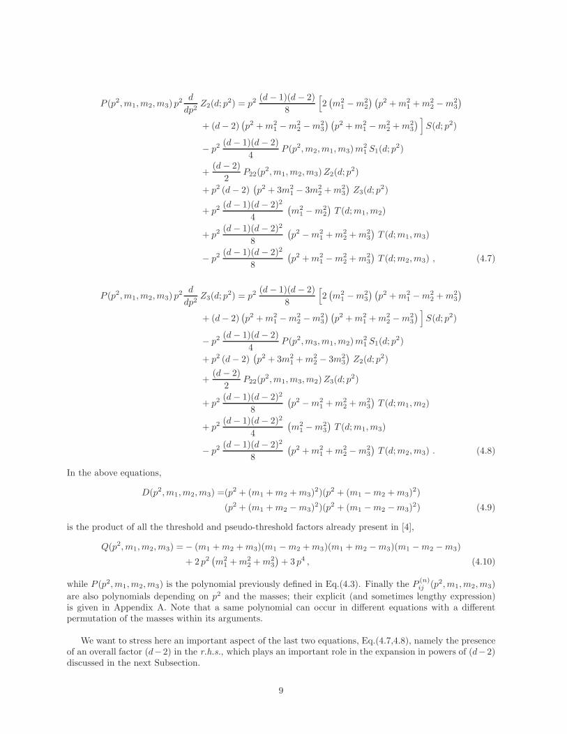
P (p2,m1,m2,m3) p2 d

dp2Z2(d; p

2) = p2(d− 1)(d− 2)

8

[

2(

m21 −m2

2

) (

p2 +m21 +m2

2 −m23

)

+ (d− 2)(

p2 +m21 −m2

2 −m23

) (

p2 +m21 −m2

2 +m23

)

]

S(d; p2)

− p2(d− 1)(d− 2)

4P (p2,m2,m1,m3)m

21 S1(d; p

2)

+(d− 2)

2P22(p

2,m1,m2,m3)Z2(d; p2)

+ p2 (d− 2)(

p2 + 3m21 − 3m2

2 +m23

)

Z3(d; p2)

+ p2(d− 1)(d− 2)2

4

(

m21 −m2

2

)

T (d;m1,m2)

+ p2(d− 1)(d− 2)2

8

(

p2 −m21 +m2

2 +m23

)

T (d;m1,m3)

− p2(d− 1)(d− 2)2

8

(

p2 +m21 −m2

2 +m23

)

T (d;m2,m3) , (4.7)

P (p2,m1,m2,m3) p2 d

dp2Z3(d; p

2) = p2(d− 1)(d− 2)

8

[

2(

m21 −m2

3

) (

p2 +m21 −m2

2 +m23

)

+ (d− 2)(

p2 +m21 −m2

2 −m23

) (

p2 +m21 +m2

2 −m23

)

]

S(d; p2)

− p2(d− 1)(d− 2)

4P (p2,m3,m1,m2)m

21 S1(d; p

2)

+ p2 (d− 2)(

p2 + 3m21 +m2

2 − 3m23

)

Z2(d; p2)

+(d− 2)

2P22(p

2,m1,m3,m2)Z3(d; p2)

+ p2(d− 1)(d− 2)2

8

(

p2 −m21 +m2

2 +m23

)

T (d;m1,m2)

+ p2(d− 1)(d− 2)2

4

(

m21 −m2

3

)

T (d;m1,m3)

− p2(d− 1)(d− 2)2

8

(

p2 +m21 +m2

2 −m23

)

T (d;m2,m3) . (4.8)

In the above equations,

D(p2,m1,m2,m3) =(p2 + (m1 +m2 +m3)2)(p2 + (m1 −m2 +m3)

2)

(p2 + (m1 +m2 −m3)2)(p2 + (m1 −m2 −m3)

2) (4.9)

is the product of all the threshold and pseudo-threshold factors already present in [4],

Q(p2,m1,m2,m3) =− (m1 +m2 +m3)(m1 −m2 +m3)(m1 +m2 −m3)(m1 −m2 −m3)

+ 2 p2(

m21 +m2

2 +m23

)

+ 3 p4 , (4.10)

while P (p2,m1,m2,m3) is the polynomial previously defined in Eq.(4.3). Finally the P(n)ij (p2,m1,m2,m3)

are also polynomials depending on p2 and the masses; their explicit (and sometimes lengthy expression)is given in Appendix A. Note that a same polynomial can occur in different equations with a differentpermutation of the masses within its arguments.

We want to stress here an important aspect of the last two equations, Eq.(4.7,4.8), namely the presenceof an overall factor (d− 2) in the r.h.s., which plays an important role in the expansion in powers of (d− 2)discussed in the next Subsection.

9

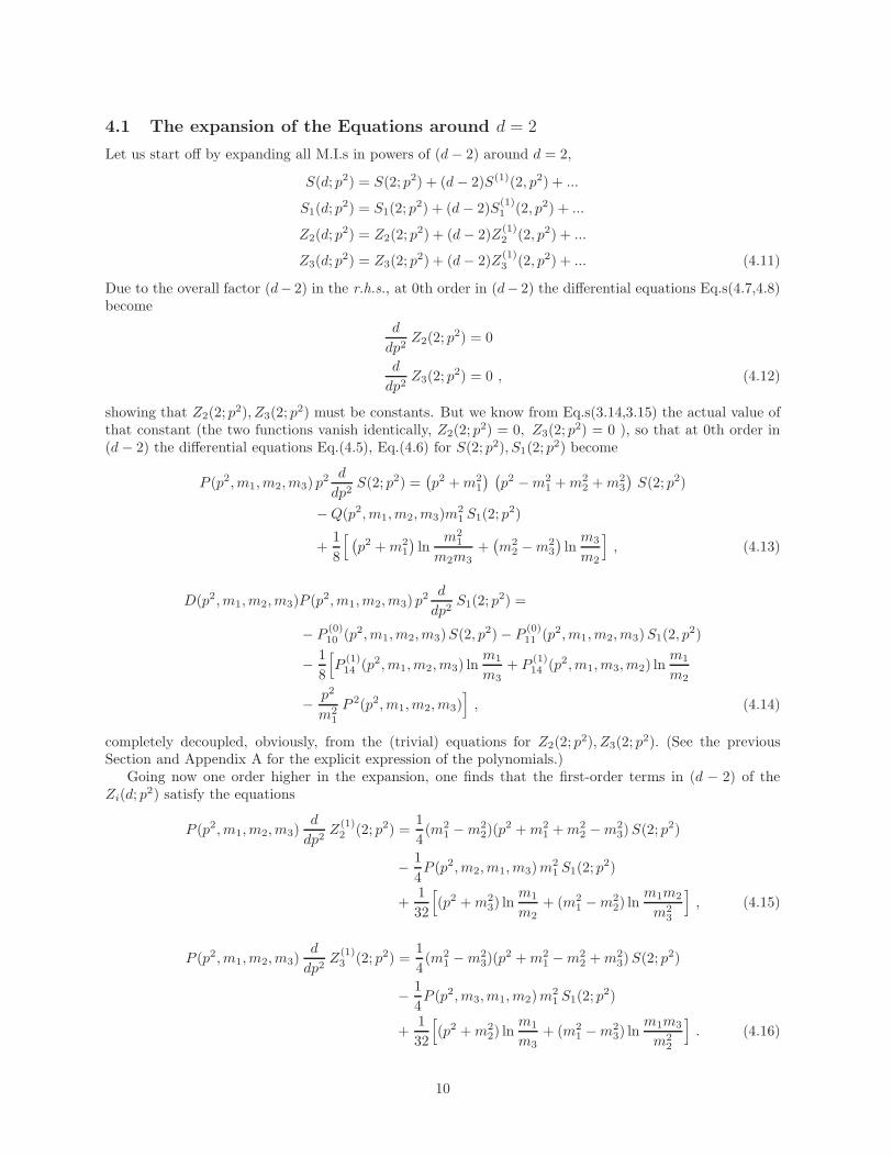
4.1 The expansion of the Equations around d = 2

Let us start off by expanding all M.I.s in powers of (d− 2) around d = 2,

S(d; p2) = S(2; p2) + (d− 2)S(1)(2, p2) + ...

S1(d; p2) = S1(2; p

2) + (d− 2)S(1)1 (2, p2) + ...

Z2(d; p2) = Z2(2; p

2) + (d− 2)Z(1)2 (2, p2) + ...

Z3(d; p2) = Z3(2; p

2) + (d− 2)Z(1)3 (2, p2) + ... (4.11)

Due to the overall factor (d− 2) in the r.h.s., at 0th order in (d− 2) the differential equations Eq.s(4.7,4.8)become

d

dp2Z2(2; p

2) = 0

d

dp2Z3(2; p

2) = 0 , (4.12)

showing that Z2(2; p2), Z3(2; p

2) must be constants. But we know from Eq.s(3.14,3.15) the actual value ofthat constant (the two functions vanish identically, Z2(2; p

2) = 0, Z3(2; p2) = 0 ), so that at 0th order in

(d− 2) the differential equations Eq.(4.5), Eq.(4.6) for S(2; p2), S1(2; p2) become

P (p2,m1,m2,m3) p2 d

dp2S(2; p2) =

(

p2 +m21

) (

p2 −m21 +m2

2 +m23

)

S(2; p2)

−Q(p2,m1,m2,m3)m21 S1(2; p

2)

+1

8

[

(

p2 +m21

)

lnm2

1

m2m3+(

m22 −m2

3

)

lnm3

m2

]

, (4.13)

D(p2,m1,m2,m3)P (p2,m1,m2,m3) p2 d

dp2S1(2; p

2) =

− P(0)10 (p2,m1,m2,m3)S(2, p

2)− P(0)11 (p2,m1,m2,m3)S1(2, p

2)

− 1

8

[

P(1)14 (p2,m1,m2,m3) ln

m1

m3+ P

(1)14 (p2,m1,m3,m2) ln

m1

m2

− p2

m21

P 2(p2,m1,m2,m3)]

, (4.14)

completely decoupled, obviously, from the (trivial) equations for Z2(2; p2), Z3(2; p

2). (See the previousSection and Appendix A for the explicit expression of the polynomials.)

Going now one order higher in the expansion, one finds that the first-order terms in (d − 2) of theZi(d; p

2) satisfy the equations

P (p2,m1,m2,m3)d

dp2Z

(1)2 (2; p2) =

1

4(m2

1 −m22)(p

2 +m21 +m2

2 −m23)S(2; p

2)

− 1

4P (p2,m2,m1,m3)m

21 S1(2; p

2)

+1

32

[

(p2 +m23) ln

m1

m2+ (m2

1 −m22) ln

m1m2

m23

]

, (4.15)

P (p2,m1,m2,m3)d

dp2Z

(1)3 (2; p2) =

1

4(m2

1 −m23)(p

2 +m21 −m2

2 +m23)S(2; p

2)

− 1

4P (p2,m3,m1,m2)m

21 S1(2; p

2)

+1

32

[

(p2 +m22) ln

m1

m3+ (m2

1 −m23) ln

m1m3

m22

]

. (4.16)

10

It is to be noted that Z(1)2 (2; p2), Z

(1)3 (2; p2) do not appear in the r.h.s. of Eq.s(4.15,4.16), which contains

only S(2; p2) and S1(2; p2), to be considered known once Eq.s(4.13,4.14) for the 0th orders in (d− 2) have

been solved. Eq.s(4.15,4.16), indeed, are absolutely trivial when considered as differential equations, as they

contain only the derivatives of Z(1)2 (2; p2), Z

(1)3 (2; p2), and can therefore be solved by a simple quadrature.

Knowing Z(1)2 (2; p2), Z

(1)3 (2; p2), one can move to the differential equations for S(1)(2; p2), S

(1)1 (2; p2)

(which we don’t write here for the sake of brevity); they involve Z(1)2 (2; p2), Z

(1)3 (2; p2) as known inhomo-

geneous terms, and form again a closed set of two differential equations, decoupled from the equations forthe other two M.I.s, as at 0th order in (d− 2).

Thanks to the overall factor (d − 2) in the r.h.s. of Eq.s(4.7,4.8), the pattern – a quadrature for

Z(k)2 (2; p2), Z

(k)3 (2; p2) and a closed set of two differential equations for S(k)(2; p2), S

(k)1 (2; p2) – is completely

general, and can be iterated, at least in principle, up to any required order k in (d− 2).

5 Second-order Differential Equation for S(d; p2)

We go back now to the system of differential equations Eq.s(4.5,4.6), for obtaining a second-order differentialequation for S(d; p2). We can use Eq.(4.5) in order to express S1(d; p

2) in function of S(d; p2) and of itsderivative, dS(d; p2)/dp2. By substituting this expression into Eq.(4.6) we can then derive a second-order differential equation for S(d; p2) only, which however still contains Z2(d; p

2) and Z3(d; p2) in the

inhomogeneous part:

A1(p2,m1,m2,m3)

(

d

dp2

)2

S(d; p2) +[

A(0)2 (p2,m1,m2,m3) + (d− 2)A

(1)2 (p2,m1,m2,m3)

] d

dp2S(d; p2)

+ (d− 3)[

A(0)3 (p2,m1,m2,m3) + (d− 2)A

(1)3 (p2,m1,m2,m3)

]

S(d; p2)

+(d− 3)

(d− 1)

[

A4(p2,m1,m2,m3)Z2(d; p

2) +A4(p2,m1,m3,m2)Z3(d; p

2)]

+ (d− 2)[

A(1)5 (p2,m1,m2,m3) + (d− 2)A

(2)5 (p2,m1,m2,m3)

]

T (d;m1,m2)

+ (d− 2)[

A(1)5 (p2,m1,m3,m2) + (d− 2)A

(2)5 (p2,m1,m3,m2)

]

T (d;m1,m3)

+ (d− 2)[

A(1)5 (p2,m2,m3,m1) + (d− 2)A

(2)5 (p2,m2,m3,m1)

]

T (d;m2,m3)

= 0 , (5.1)

where A1(p2,m1,m2,m3) = p2 D(p2,m2

1,m22,m

23)P (p2,m1,m2,m3) , with D(p2,m2

1,m22,m

23) and

P (p2,m1,m2,m3) being the usual polynomials defined by Eq.s(4.3,4.9). The A(n)j (p2,m1,m2,m3) are also

polynomials which depend on the three masses and on p2, but do not depend on the dimensions d. Theirexplicit expressions, as usual quite lengthy, can be found in Appendix B.

The equation above is exact in d but contains, besides S(d; p2) and its derivatives, also Z2(d; p2) and

Z3(d; p2) as inhomogeneous terms. Nevertheless, recalling once more that Z2(2; p

2) = Z3(2; p2) = 0, we

can expand Eq.(5.1) in powers of (d− 2) and obtain at leading order in (d− 2) a second-order differentialequation for S(2; p2) only :

A1(p2,m1,m2,m3)

(

d

dp2

)2

S(2; p2) +A(0)2 (p2,m1,m2,m3)

(

d

dp2

)

S(2; p2)

−A(0)3 (p2,m1,m2,m3)S(2; p

2) +1

4

[

A(2)5 (p2,m1,m2,m3)

+A(2)5 (p2,m1,m3,m2) +A

(2)5 (p2,m2,m3,m1)

+A(1)5 (p2,m1,m2,m3) ln

(

m1

m3

)

+A(1)5 (p2,m1,m3,m2) ln

(

m1

m2

)

]

= 0 , (5.2)

11

where we made use of the relation Eq.(B.8) of Appendix B. We compared Eq.(5.2) with the second-orderdifferential equation derived in [9], finding perfect agreement. Eq.(5.2) has been solved in reference [10] interms of one-dimensional integrals over elliptic integrals.

Upon inserting the result in Eq.(4.13) one can obtain S1(2; p2) in terms of S(2; p2) and dS(2; p2)/dp2.

Inserting then S(2; p2) and S1(2; p2) in Eq.s(4.15, 4.16), one obtains by quadrature the first-order terms,

Z(1)2 (2; p2) and Z

(1)3 (2; p2), of the expansion in (d− 2) of Z2(d; p

2) and Z3(d; p2).

Having these results on hand, we can now consider the first-order in (d − 2) of the Eq.(5.1), which isnow a second-order differential equation for S(1)(2; p2) only, with known inhomogeneous terms (namely

S(2; p2), Z(1)2 (2; p2) and Z

(1)3 (2; p2)). Proceeding in this way, at least in principle, the whole procedure can

be iterated up to any required order in (d− 2).

6 Shifting relations from d = 2 to d = 4 dimensions

In the previous Sections we have shown how to use the Schouten identities for writing the differentialequations for the M.I.s of the massive sunrise at d = 2 dimensions in block form, and outlined the procedurefor obtaining iteratively all the coefficients of the expansion in (d − 2) of the four M.I.s starting from asecond-order differential equation for S(2; p2), the leading term of the expansion.

The physically interesting case corresponds however to the expansion of the M.I.s for d ≈ 4; we havetherefore to convert the information given by the expansion at d ≈ 2 in useful information at d ≈ 4.

As it is well known, quite in general one can relate any Feynman integral evaluated in d dimensions tothe very same integral evaluated in (d− 2) dimensions by means of the Tarasov’s shifting relation [7]. Thisdimensional shift is achieved by acting on the Feynman integral with a suitable combination of derivativeswith respect to the internal masses. In the case of the “conventional ” M.I.s of the sunrise graph, as definedin Eq.(3.7), the shifting relations read:

S(d− 2; p2) =22

(d− 6)∆S(d; p2) ,

Si(d− 2; p2) =22

(d− 6)∆Si(d; p

2) , i = 1, 2, 3 , (6.1)

where the differential operator ∆ takes the form:

∆ =∂

∂m21

∂

∂m22

+∂

∂m21

∂

∂m23

+∂

∂m22

∂

∂m23

. (6.2)

Carrying out the derivatives in the integral representation for the four M.I.s of Eq.(3.7), one obtains acombination of integrals which are still related to the sunrise graph. They can be expressed in terms of thefull set of M.I.s in d dimensions (by full set we mean the four M.I.s and the tadpoles); one obtains in thatway a set of four equations which explicitly relate the four M.I.s of the sunrise graph evaluated in (d − 2)dimensions to suitable combinations of the same integrals (and of the tadpoles) evaluated in d dimensions.In that direct form the shifting relations would be of no practical use in our case, as they might give theM.I.s at (d− 2) ≈ 2 in terms of those (less known) at d ≈ 4.

It is however straightforward to invert the system and, in this way, to obtain the inverse shifting relations,expressing the four M.I.s in d+2 ≈ 4 dimensions in function of those in d ≈ 2 dimensions. In addition, wecan also use Eq.s(4.1,4.2) for expressing S2(d; p

2) and S3(d; p2), in terms of S(d; p2), S1(d; p

2) and Z2(d; p2),

Z3(d; p2). As a result one arrives at expressing any of the four “conventional” M.I.s S(d+2, p2), Si(d+2; p2),

i = 1, 2, 3, as a linear combination (whose coefficients depend – and in a non trivial way – on d and thekinematical variables of the problem) of the “new” M.I.s S(d; p2), S1(d; p

2), Z2(d; p2) and Z3(d; p

2) (andthe tadpoles). Indicating for simplicity the four “conventional” M.I.s with Mi(d) and with Nj(d) the four“new” M.I.s and the tadpoles, and ignoring for ease of notation all the kinematical variables, the inverse

shifting relations can be written as

Mi(d+ 2) =∑

j

Ci,j(d)Nj(d) . (6.3)

12

Given a relation of the formF (d+ 2) = G(d) ,

by expanding around d = 2 one has, quite in general

F (d+ 2) =

p∑

n=r

(d− 2)n F (n)(4) ,

G(d) =

p∑

n=r

(d− 2)n G(n)(2) ,

where r, the first value of the summation index, can be negative (as it is the case in a Laurent expansion),so that

F (n)(4) = G(n)(2) .

In the case of the inverse shift Eq.(6.3), one has that the coefficients of the expansion of the “conventional”M.I.s in (d − 4) for d ≈ 4 are completely determined by those of the expansion in (d − 2) for d ≈ 2 ofthe “new” M.I.s, discussed in the previous Sections, and of the tadpoles (expanding around d = 2 the twosides of Eq.(6.3) requires also the expansion of the coefficients Ci,j(d), but that is not a problem once theinverse shift has been written down explicitly).

The explicit formulas of the direct or inverse shifting relations are easily obtained but very lengthy andwe decided not to include them entirely here for the sake of brevity. For what follows, it is sufficient todiscuss only the general features of one of the inverse shifting relations, namely the relation expressingS(d+ 2; p2) in terms of S(d; p2), S1(d; p

2) and Z2(d; p2), Z3(d; p

2). Keeping for simplicity only the leadingterm of the expansion in (d− 2) of the coefficients we find:

S(d+ 2; p2) =[

C(p2,m1,m2,m3) +O (d− 2)]

S(d; p2)

+[

C1(p2,m1,m2,m3) +O (d− 2)

]

S1(d; p2)

+

[

1

d− 2C2(p

2,m1,m2,m3) +O (1)

]

Z2(d; p2)

+

[

1

d− 2C3(p

2,m1,m2,m3) +O (1)

]

Z3(d; p2)

+[

C(0)4 (p2,m1,m2,m3) +O (d− 2)

]

T (d;m1,m2)

+[

C(0)5 (p2,m1,m2,m3) +O (d− 2)

]

T (d;m1,m2)

+[

C(0)6 (p2,m1,m2,m3) +O (d− 2)

]

T (d;m1,m2) . (6.4)

In the formula above the C(p2,m1,m2,m3), Ci(p2,m1,m2,m3), are ratios of suitable polynomials which, as

usual, depend on p2 and on the three masses but, most importantly, do not depend on the dimensions d. Theexplicit expressions for C(p2,m1,m2,m3), C1(p

2,m1,m2,m3), C2(p2,m1,m2,m3) and C3(p

2,m1,m2,m3),which will also be used in the following, can be found in Appendix C, Eq.s(C.2-C.5). Note anyway that:

C3(p2,m1,m2,m3) = C2(p

2,m1,m3,m2) .

By writing the expansion of S(d+ 2; p2) at d ≈ 2 as

S(d+ 2; p2) =∑

n

S(n)(4; p2)(d − 2)n , (6.5)

and then expanding Eq.(6.4) at d ≈ 2, one recovers the expression of the coefficients S(n)(4; p2) in terms ofthe coefficients of the expansion of the four M.I.s and the tadpoles in (d− 2).

A few observations are in order. Eq.(6.4) exhibits an explicit pole in 1/(d− 2) only in the coefficientsof Z2(d; p

2) and Z3(d; p2); recalling once more that at d = 2 both Z2(2; p

2) and Z3(2; p2) are identically

13

zero, see Eq.s(3.14,3.15), it is clear that these poles will not generate any singularity of S(d; p2) as d → 2.On the other hand, the tadpoles in the r.h.s. of Eq.(6.4) do generate polar singularities of S(d + 2; p2);recalling Eq.s(3.5,3.6) and by using the lengthy explicit form of the coefficients (which we did not write forbrevity) one finds immediately

S(−2)(4; p2) = − (m21 +m2

2 +m23)

8,

S(−1)(4; p2) =1

32

[

p2 + 6(

m21 +m2

2 +m23

)

]

− 1

8

[

m21 ln (m2

1) +m22 ln (m2

2) +m23 ln (m2

3)]

, (6.6)

formulas already known for a long time in the literature [4].As a second observation, let us look at the zeroth-order term S(0)(4; p2) of S(d; p2) in (d − 4), i.e.

the zeroth-order term in (d − 2) of Eq.(6.4). We have already commented the apparent polar singularity1/(d− 2) in the coefficients of Z2(d; p

2) and Z3(d; p2), actually absent because Z2(2; p

2) and Z3(2; p2) are

both vanishing. But due to the presence of the 1/(d− 2) polar factor, in order to recover the zeroth-orderterm S(0)(4; p2), one needs, besides S(2; p2), S1(2; p

2), also the first-order of the corresponding expansion of

Z2(d; p2) and Z3(d; p

2), namely Z(1)2 (2; p2) and Z

(1)3 (2; p2) – obtained, in our approach, from the systematic

expansion of the differential equations, see Eq.s(4.15,4.16) or Section 5.The complete expression of S(0)(4; p2), which is rather cumbersome, is given by Eq.(C.1) of Appendix C.

The corresponding formulas for the other three M.I.s, i.e. the Si(d+ 2; p2), can be obtained directly fromthe authors.

7 The imaginary parts of the Master Integrals.

In this Section, which is somewhat pedagogical, we discuss the relationship between the imaginary partsof the M.I.s at d = 2 and d = 4 dimensions, as a simple but explicit example of functions exhibiting theproperties described in the previous sections.

At d = 2 the Cutkosky-Veltman rule [14, 15] gives for S(d; p2), as defined by the first of Eq.s(3.7),

1

πImS(2;−W 2) = N2

∫ b3

b2

db1

√

R4(b; b1, b2, b3, b4), (7.1)

where the following notations were introduced:

N2 = 1/2

p2 = −W 2, W ≥ m1 +m2 +m3 ,

(m2 −m3)2 = b1 ≤ (m2 +m3)

2 = b2 ≤ (W −m1)2 = b3 ≤ (W +m1)

2 = b4 ,

R4(b; b1, b2, b3, b4) = (b− b1)(b − b2)(b3 − b)(b4 − b) . (7.2)

We have the relationR4(b; b1, b2, b3, b4) = R2(b,m

22,m

23) R2(W

2, b,m21) , (7.3)

whereR2(a, b, c) = a2 + b2 + c2 − 2ab− 2ac− 2bc , (7.4)

is the familiar invariant form appearing in the two-body phase space, showing that the system of the threeparticles, whose masses enter in the definition of R4(b; b1, b2, b3, b4), can be considered as the merging ofa two-body system of total energy

√b and masses m2,m3 with a two-body system of total energy W and

masses√b,m1 .

According to Eq.s(3.7), for i=1,2,3

1

πImSi(2;−W 2) = − d

dm2i

(

1

πImS(2;−W 2)

)

; (7.5)

14

the integral representation Eq.(7.1), however, is of no use for obtaining ImSi(2;−W 2) through a directdifferentiation (due to the appearance of end point singularities). It is more convenient to use Eq.(D.13)of the Appendix D, so that Eq.(7.1) becomes

1

πImS(2;−W 2) = N2

2√

(b4 − b2)(b3 − b1)K(w2) , (7.6)

where K(w2) is the complete elliptic integral of the first kind, Eq.(D.6), and

w2 =(b4 − b1)(b3 − b1)

(b4 − b2)(b3 − b1)

=(W +m1 +m2 −m3)(W +m1 −m2 +m3)(W −m1 +m2 −m3)(W −m1 −m2 +m3)

(W +m1 +m2 +m3)(W +m1 −m2 −m3)(W −m1 +m2 −m3)(W −m1 −m2 +m3),

(b4 − b2)(b3 − b1) = (W +m1 +m2 +m3)(W +m1 −m2 −m3)

× (W −m1 +m2 −m3)(W −m1 −m2 +m3) . (7.7)

Let us observe, in passing, that, even if ImS(2,−W 2) (and, more generally S(d; p2) as well) is obviouslysymmetric in the three masses m1,m2,m3, the symmetry is not explicitly shown by the integral represen-tation Eq.(7.1), while the manifest symmetry is restored in Eq.s(7.6,7.7).One can now use Eq.(7.6) and Eq.(D.11) to carry out the derivative with respect to the masses m2

i inEq.(7.5); the result reads

1

πImS1(2;−W 2) = N2

1

2m21

√

(b3 − b1)(b4 − b2)

1

(b3 − b2)(b4 − b1)

×[

4m1(m1m23 +m1m

22 −m3

1 + 2m2m3W +m1W2)K(w2)

−P (−W 2,m1,m2,m3)E(w2)]

, (7.8)

1

πImS2(2;−W 2) = N2

1

2m22

√

(b3 − b1)(b4 − b2)

1

(b3 − b2)(b4 − b1)

×[

4m2(m2m23 +m2m

21 −m3

2 + 2m1m3W +m2W2)K(w2)

−P (−W 2,m2,m1,m3)E(w2)]

, (7.9)

1

πImS3(2;−W 2) = N2

1

2m23

√

(b3 − b1)(b4 − b2)

1

(b3 − b2)(b4 − b1)

×[

4m3(m3m21 +m3m

22 −m3

3 + 2m2m1W +m3W2)K(w2)

−P (−W 2,m3,m2,m1)E(w2)]

, (7.10)

where w2 is given by the first of Eq.s(7.7), P (p2,m1,m2,m3) is the polynomial already introduced inEq.(4.3), symmetric in the last two arguments, and E(w2) is the complete elliptic integral of the secondkind, see Eq.(D.7).

Eq.s(7.6,7.8,7.9,7.10) express the four quantities ImS(2;−W 2), ImSi(2,−W 2), i = 1, 2, 3 in terms ofjust two functions, the elliptic integrals K(w2), E(w2); therefore, the four imaginary parts cannot be alllinearly independent. It is indeed easy to check that they satisfy the two equations

− 1

12(m2

1 − 2m22 +m2

3) ImS(2;−W 2) +1

12(−W 2 +m2

1 − 3m22 + 3m2

3) m21 ImS1(2,−W 2)

− 1

6(−W 2 +m2

2) m22 ImS2(2;−W 2) +

1

12(−W 2 + 3m2

1 − 3m22 +m2

3) m23 ImS3(2;−W 2) = 0 ,

− 1

12(m2

1 +m22 − 2m2

3) ImS(2;−W 2) +1

12(−W 2 +m2

1 + 3m22 − 3m2

3) m21 ImS1(2;−W 2)

+1

12(−W 2 + 3m2

1 +m22 − 3m2

3) m22 ImS2(2;−W 2)− 1

6(−W 2 +m2

3) m23 ImS3(2;−W 2) = 0 ,

15

which are nothing but the imaginary parts of Z2(2;−W 2), Z3(2;−W 2), Eq.s(3.14,3.15).As a further comment on the imaginary parts at d = 2, let us observe that they take a finite value at

threshold, i.e. in the W → (m1 +m2 +m3) limit. In that limit, indeed, b3 → b2 = (m2 +m3)2, and one

finds∫ b3

b2

db√

R4(b; b1, b2, b3, b4)→ 1√

(b2 − b1)(b4 − b2)

∫ b3

b2

db√

(b− b2)(b3 − b)=

π√

(b2 − b1)(b4 − b2),

so that1

πImS(2;−W 2) −−−−−−−−−−−−→

W→(m1+m2+m3)

N2

4√

m1m2m3(m1 +m2 +m3). (7.11)

The extension to the value at threshold of the ImSi(2,−W 2) is similar, even if requiring one more termin the expansion due to the presence of the denominator 1/(b3 − b2) in their definitions, Eq.s(7.8,7.9,7.10).The threshold values are

1

πImS1(2;−W 2) −−−−−−−−−−−−→

W→(m1+m2+m3)

N2

32

(

− 3

m1+

1

m2+

1

m3− 1

m1 +m2 +m3

)

1√

m1m2m3(m1 +m2 +m3),

1

πImS2(2;−W 2) −−−−−−−−−−−−→

W→(m1+m2+m3)

N2

32

(

+1

m1− 3

m2+

1

m3− 1

m1 +m2 +m3

)

1√

m1m2m3(m1 +m2 +m3),

1

πImS3(2;−W 2) −−−−−−−−−−−−→

W→(m1+m2+m3)

N2

32

(

+1

m1+

1

m2− 3

m3− 1

m1 +m2 +m3

)

1√

m1m2m3(m1 +m2 +m3). (7.12)

At d = 4 the imaginary part of S(d; p2), by using the same notation as in Eq.(7.1), is given by

1

πImS(4;−W 2) = N4

∫ b3

b2

db1

b

√

R4(b; b1, b2, b3, b4) . (7.13)

with

N4 =1

8W 2. (7.14)

At variance with the d = 2 case, the ImSi(4,−W 2) can be obtained at once by differentiating with respectto the masses the previous integral representation for ImS(4;−W 2). The result can be most convenientlyexpressed in terms of the four (independent) integrals I(−1,W ), I(0,W ), I(1,W ), I(2,W ), defined (seeEq.(D.3) and the Appendix for more details and the relation to the standard complete elliptic integrals)through

I(n,W ) =

∫ b3

b2

db bn1

√

R4(b; b1, b2, b3, b4). (7.15)

An explicit calculation gives

1

πImS(4;−W 2) = N4

[

b1b2b3b4 I(−1,W )

− 3

4(b2b3b4 + b1b3b4 + b1b2b4 + b1b2b3) I(0,W )

+1

2(b3b4 + b2b4 + b2b3 + b1b4 + b1b3 + b1b2) I(1,W )

− 1

4(b1 + b2 + b3 + b4) I(2,W )

]

(7.16)

16

1

πImS1(4;−W 2) = N4

[

b1b2(

−(b4 − b3)W + (b4 + b3)m1

)

I(−1,W )

+(

(b2 + b1)(b4 − b3)W − (b2b4 + b2b3 + b1b4 + b1b3 + 2b1b2)m1

)

I(0,W )

+(

(b4 − b3)W + (b4 + b3 + 2b2 + 2b1)m1

)

I(1,W )

− 2m1 I(2,W )]

(7.17)

1

πImS2(4;−W 2) = N4

[

b3b4(

−(b2 − b1)m3 + (b2 + b1)m2

)

I(−1,W )

+(

−(2b3b4 + b2b4 + b2b3 + b1b4 + b1b3)m2 + (b2 − b1)(b4 + b3)m3

)

I(0,W )

+(

(2b4 + 2b3 + b2 + b1)m2 − (b2 − b1)m3

)

I(1,W )

− 2m2 I(2,W )]

(7.18)

1

πImS3(4;−W 2) = N4

[

b3b4(

−(b2 − b1)m2 + (b2 + b1)m3

)

I(−1,W )

+(

−(2b3b4 + b2b4 + b2b3 + b1b4 + b1b3)m3 + (b2 − b1)(b4 + b3)m2

)

I(0,W )

+(

(2b4 + 2b3 + b2 + b1)m3 − (b2 − b1)m2

)

I(1,W )

− 2m3 I(2,W )]

(7.19)

Again at variance with the d = 2 case, the four imaginary parts are now combinations of four independentelliptic integrals, and therefore all independent of each other.

Having recalled the main features of the imaginary parts of the M.I.s at d = 2 and d = 4 dimensions,we can look at the way the Tarasov’s shifting relations work in their case.

Let us start from the “direct” shift expressing the imaginary parts at d = 2 in terms of those atd = 4. The d → 4 limit of the shifting relations is trivial, even if the relevant formulas are as usual ratherlengthy. Keeping only the imaginary parts of the master integrals one finds for the M.I. S(2, p2), with−p2 = W 2 ≥ (m1 +m2 +m3)

2

1

πImS(2,−W 2) = A(W,m1,m2,m3)

1

πImS(4,−W 2)

+ B(W,m1,m2,m3)m11

πImS1(4,−W 2)

+ B(W,m2,m3,m1)m21

πImS2(4,−W 2)

+ B(W,m3,m1,m2)m31

πImS3(4,−W 2) , (7.20)

where

A(W,m1,m2,m3) = A(W,m1,m2,m3) +A(W,m1,−m2,m3)

+ A(W,m1,m2,−m3) +A(W,m1,−m2,−m3) ,

B(W,m1,m2,m3) = B(W,m1,m2,m3) +B(W,m1,−m2,m3)

+ B(W,m1,m2,−m3) +B(W,m1,−m2,−m3) ,

A(W,m1,m2,m3) =1

2m1m2m3

m1 +m2 +m3

W 2 − (m1 +m2 +m3)2,

B(W,m1,m2,m3) =1

2(2m1 +m2 +m3)A(W,m1,m2,m3) . (7.21)

Eq.(7.20) is relatively simple, and, when substituting in it the explicit values of ImS(4,−W 2) and ImSi(4,−W 2),as given by Eq.s(7.16–7.19), Eq.(7.1) is recovered. The same happens for ImSi(2,−W 2), i = 1, 2, 3 aswell.

17

Conversely, one can look at the inverse formulas, giving the imaginary parts at d + 2 → 4 in terms ofthe imaginary parts at d → 2. For ImS(4,−W 2), taking only the imaginary part at d = 2 of Eq.(6.4), oneobtains:

1

πImS(4;−W 2) = C(−W 2,m1,m2,m3)

1

πImS(2;−W 2)

+ C1(−W 2,m1,m2,m3)1

πImS1(2;−W 2)

+ C2(−W 2,m1,m2,m3)1

πImZ

(1)2 (2;−W 2)

+ C3(−W 2,m1,m2,m3)1

πImZ

(1)3 (2;−W 2) , (7.22)

where the C(−W 2,m1,m2,m3), Ci(−W 2,m1,m2,m3) have been defined in the previous section, and theirexplicit expressions can be found in Eq.s(C.2-C.5), ImS(2;−W 2), ImS1(2;−W 2) are the imaginary parts

of the corresponding Master Integrals at d = 2, while ImZ(1)2 (2;−W 2), ImZ

(1)3 (2;−W 2) are the imaginary

parts of the first term of the expansion in (d−2) of the corresponding functions, see Eq.s(4.11) (let us recallonce more that according to Eq.s(3.14,3.15) Z2(2; p

2), Z3(2; p2) vanish identically). An equation similar to

Eq.(7.22) holds for ImS1(4;−W 2); we do not write it explicitly for the sake of brevity.The functions ImS(4;−W 2), ImS1(4;−W 2) and ImS(2;−W 2), ImS1(2;−W 2) are known, see Eq.s(7.16,7.17)and Eq.s(7.6,7.8); by combining Eq.(7.22) and the similar (not written) equation for ImS1(4;−W 2), one

can obtain the explicit values of ImZ(1)2 (2;−W 2), ImZ

(1)3 (2;−W 2). One finds

1

πImZ

(1)2 (2;−W 2) =

N2

16

[

(W 2 −m23 +m2

2 −m21)I(0,W ) + I(1,W )

− (m23 −m2

2)(W2 −m2

1)I(−1,W )]

, (7.23)

1

πImZ

(1)3 (2;−W 2) =

N2

16

[

(W 2 +m23 −m2

2 −m21)I(0,W ) + I(1,W )

+ (m23 −m2

2)(W2 −m2

1)I(−1,W )]

, (7.24)

From the previous equations and the same procedure giving Eq.s(7.11,7.12) we obtain in particular thevalues at threshold

1

πImZ

(1)2 (2;−W 2) −−−−−−−−−−−−→

W→(m1+m2+m3)

N2

16

√

m2(m1 +m2 +m3)

m1 m3

1

πImZ

(1)3 (2;−W 2) −−−−−−−−−−−−→

W→(m1+m2+m3)

N2

16

√

m3(m1 +m2 +m3)

m1 m2. (7.25)

ImZ(1)2 (2;−W 2) can also be evaluated solving, by quadrature, the imaginary part of the differential

equation Eq.(4.15), i.e. by evaluating

ImZ(1)2 (2;−W 2) = C +

∫ −W 2

dp2 Im

(

d

dp2Z

(1)2 (2; p2)

)

,

where C is an integration constant and dZ(1)2 (2; p2)/dp2 is obtained from Eq.(4.15) itself. The constant

C can be fixed, a posteriori, by requiring that the imaginary parts of the “conventional” M.I. vanish atthreshold in d = 4 dimensions, a condition which leads again to Eq.s(7.25).

18

After many algebraic simplifications, one obtains for ImZ(1)2 (2;−W 2)

1

πImZ

(1)2 (2;−W 2) =

N2

16

√

m2(m1 +m2 +m3)

m1m3

+1

64

∫ W 2

(m1+m2+m3)2ds[

F (s,m1,m2,m3) I(0, s)

− G(s,m1,m2,m3) I(1, s)

+ H(s,m1,m2,m3) I(2, s)]

. (7.26)

where the three quantities F , G, H are all expressed in terms of the corresponding functions F,G,H by therelation

F (s,m1,m2,m3) = F (s,m1,m2,m3) + F (s,m1,−m2,m3)

+ F (s,m1,m2,−m3) + F (s,m1,−m2,−m3) ,

and the explicit expressions of those functions are

F (s,m1,m2,m3) =(m2 +m3)

2

m1m3

2m21 +m2

2 +m23 + 2m1m2 + 2m1m3

s− (m1 +m2 +m3)2,

G(s,m1,m2,m3) = 2m2

1 +m22 +m2

3 +m1m2 +m1m3 +m2m3

m1m3 [s− (m1 +m2 +m3)2],

H(s,m1,m2,m3) =1

m1m3 [s− (m1 +m2 +m3)2].

To carry out the integration, we use the integral representations Eq.(D.4) for the elliptic integrals I(n, s)and exchange the order of integration according to

∫ W 2

(m1+m2+m3)2ds

∫ (√s−m1)

2

(m2+m3)2

db√

R4(b; b1, b2, b3, b4)=

∫ (W−m1)2

(m2+m3)2

db√

R2(b,m22,m

23)

∫ W 2

(√b+m1)2

ds√

R2(s, b,m21)

,

where Eq.(7.3) was used. The s integration is then elementary, giving only logarithms of suitable argumentsand new square roots quadratic in b ; a subsequent integration by parts in b removes those logarithms withsome of the accompanying square roots, and the result is Eq.(7.23), as expected.

The same applies also for ImZ(1)3 (2;−W 2), whose value is obtained by simply exchanging m2 and m3 in

Eq.(7.23).

8 Conclusions

In this paper we introduced a new class of identities, dubbed Schouten identities, valid at fixed integervalue of the dimensions d. We applied the identities valid at d = 2 to the case of the massive two-loopsunrise graph with different masses, finding that in d = 2 dimensions only two of the four Master Integrals(M.I.s) are actually independent, so that the other two can be expressed as suitable linear combinations ofthe latter.

In the general case of arbitrary dimension d and different masses, the four M.I.s are known to fulfil asystem of four first-order coupled differential equations in the external momentum transfer. The systemcan equivalently be re-phrased as a fourth-order differential equation for one of the M.I.s only.

Using these relations we introduced a new set of four independent M.I.s, valid for any number ofdimensions d, whose property is that two of the newly defined integrals vanish identically in d = 2. Thenew system of differential equations for this set of M.I.s takes then a simpler block form when expanded in(d− 2).

19

Starting from this system, one can derive a second-order differential equation, exact in d, for the fullscalar amplitude, which still contains the two integrals, whose value is zero at d = 2, as inhomogeneousterms. We verified that the zeroth-order of our equation corresponds to the equation derived in [9]. Ourequations, once expanded in powers of (d − 2), can be used, together with the linear equations for theremaining three M.I.s, for evaluating recursively, at least in principle, all four M.I.s, up to any order in(d− 2).

We then worked out explicitly the Tarasov’s shifting relations needed to recover the physically morerelevant value of the four M.I.s expanded in (d− 4) at d ≈ 4 starting from the expansion in (d− 2) at d ≈ 2worked out in our approach.

As an example of this procedure we discussed the relationship between the imaginary parts of the fourM.I.s in d = 2 and d = 4. The latter can be computed using the Cutkosky-Veltman rule. We showed howin d = 2 the imaginary parts of the four M.I.s can be written in terms of two independent functions only,namely the complete elliptic integrals of the first and of the second kind. The same is not true in d = 4dimensions, where four independent elliptic integrals are needed in order to represent the four imaginaryparts. We then showed how the Tarasov’s shift formulas relate the imaginary parts in d = 2 and d = 4dimensions. Finally, we gave an explicit example of how the differential equations for the imaginary partsof the master integrals can be integrated by quadrature.

Acknowledgements

We are grateful to J.Vermaseren for his assistance in the use of the algebraic program FORM [17] whichwas intensively used in all the steps of the calculation, to T.Gehrmann for many interesting commentsand discussions, and to F.Cascioli for proofreading the whole manuscript. L.T. wishes to thank A. vonManteuffel for his assistance with Reduze 2 [18], with which the reduction to Master Integrals of thetwo-loop sunrise has been carried out, and G.Heinrich and S. Borowka for their help with SecDec [13].This research was supported in part by the Swiss National Science Foundation (SNF) under the contractPDFMP2-135101.

A The polynomials of the first-order differential equations

In this appendix we give the explicit expressions for the polynomials appearing in the first-order differentialequations in section 4. All polynomials are functions of p2 and of the three masses m1, m2, m3, while theydo not depend on the dimensions d.

P(0)10 (p2,m1,m2,m3) = −m2

1(m1 +m2 +m3)(m1 −m2 +m3)(m1 +m2 −m3)(m1 −m2 −m3)

×(

m21 −m2

2 −m23

)2

+ p2(

m81 + 4m2

2m61 − 14m4

2m41 + 12m6

2m21 − 3m8

2 + 4m23m

61 + 4m2

3m42m

21

−8m23m

62 − 14m4

3m41 + 4m4

3m22m

21 + 22m4

3m42 + 12m6

3m21 − 8m6

3m22 − 3m8

3

)

+ p4(

10m61 − 4m2

2m41 + 2m4

2m21 − 8m6

2 − 4m23m

41 + 16m2

3m42 + 2m4

3m21

+16m43m

22 − 8m6

3

)

+ p6(

14m41 − 4m2

2m21 − 6m4

2 − 4m23m

21 + 24m2

3m22 − 6m4

3

)

+ 7p8m21 + p10 , (A.1)

20

P(1)10 (p2,m1,m2,m3) = (m1 +m2 +m3)(m1 −m2 +m3)(m1 +m2 −m3)(m1 −m2 −m3)

×(

m21 −m2

2 −m23

) (

7m41 − 6m2

2m21 −m4

2 − 6m23m

21 + 2m2

3m22 −m4

3

)

+ p2(

11m81 − 48m2

2m61 + 78m4

2m41 − 56m6

2m21 + 15m8

2 − 48m23m

61

+68m23m

22m

41 − 40m2

3m42m

21 + 20m2

3m62 + 78m4

3m41 − 40m4

3m22m

21

−70m43m

42 − 56m6

3m21 + 20m6

3m22 + 15m8

3

)

+ p4(

−2m61 − 14m2

2m41 + 2m4

2m21 + 14m6

2 − 14m23m

41 + 60m2

3m22m

21

−62m23m

42 + 2m4

3m21 − 62m4

3m22 + 14m6

3

)

− 2 p6(

m21 −m2

2 − 3m23

) (

m21 − 3m2

2 −m23

)

+ p8(

11m21 +m2

2 +m23

)

+ 7 p10 , (A.2)

P(2)10 (p2,m1,m2,m3) = (m1 +m2 +m3)(m1 −m2 +m3)(m1 +m2 −m3)(m1 −m2 −m3)

×(

5m41 − 4m2

2m21 −m4

2 − 4m23m

21 + 2m2

3m22 −m4

3

)

+ p2(

8m61 − 18m2

2m41 + 20m4

2m21 − 10m6

2 − 18m23m

41 + 24m2

3m22m

21

+10m23m

42 + 20m4

3m21 + 10m4

3m22 − 10m6

3

)

+ p4(

10m41 + 6m2

2m21 − 8m4

2 + 6m23m

21 + 48m2

3m22 − 8m4

3

)

+ p6(

16m21 + 10m2

2 + 10m23

)

+ 9 p8 , (A.3)

P(0)11 (p2,m1,m2,m3) = (m1 +m2 +m3)

2(m1 −m2 +m3)2(m1 +m2 −m3)

2(m1 −m2 −m3)2

×(

m21 −m2

2 −m23

)

m21

+ p2(

−6m101 +m2

2m81 + 32m4

2m61 − 42m6

2m41 + 14m8

2m21 +m10

2 +m23m

81

−64m23m

22m

61 + 26m2

3m42m

41 + 40m2

3m62m

21 − 3m2

3m82 + 32m4

3m61

+26m43m

22m

41 − 108m4

3m42m

21 + 2m4

3m62 − 42m6

3m41 + 40m6

3m22m

21

+2m63m

42 + 14m8

3m21 − 3m8

3m22 +m10

3

)

+ p4(

−33m81 + 6m2

2m61 − 20m4

2m41 + 42m6

2m21 + 5m8

2 + 6m23m

61

−24m23m

22m

41 − 26m2

3m42m

21 − 4m2

3m62 − 20m4

3m41 − 26m4

3m22m

21

−2m43m

42 + 42m6

3m21 − 4m6

3m22 + 5m8

3

)

+ p6(

−52m61 − 6m2

2m41 + 32m4

2m21 + 10m6

2 − 6m23m

41 − 64m2

3m22m

21

+6m23m

42 + 32m4

3m21 + 6m4

3m22 + 10m6

3

)

+ p8(

−33m41 −m2

2m21 + 10m4

2 −m23m

21 + 12m2

3m22 + 10m4

3

)

+ p10(

−6m21 + 5m2

2 + 5m23

)

+ p12 , (A.4)

21

P(1)11 (p2,m1,m2,m3) = (m1 +m2 +m3)

2(m1 −m2 +m3)2(m1 +m2 −m3)

2(m1 −m2 −m3)2

×(

5m41 − 4m2

2m21 −m4

2 − 4m23m

21 + 2m2

3m22 −m4

3

)

+ p2(

2m101 − 28m2

2m81 + 76m4

2m61 − 80m6

2m41 + 34m8

2m21

−4m102 − 28m2

3m81 + 40m2

3m22m

61 − 48m2

3m42m

41 + 24m2

3m62m

21

+12m23m

82 + 76m4

3m61 − 48m4

3m22m

41 − 116m4

3m42m

21 − 8m4

3m62

−80m63m

41 + 24m6

3m22m

21 − 8m6

3m42 + 34m8

3m21 + 12m8

3m22 − 4m10

3

)

+ p4(

−41m81 − 42m4

2m41 + 88m6

2m21 − 5m8

2 + 52m23m

22m

41 − 152m2

3m42m

21

+4m23m

62 − 42m4

3m41 − 152m4

3m22m

21 + 2m4

3m42 + 88m6

3m21 + 4m6

3m22 − 5m8

3

)

+ p6(

−84m61 − 8m2

2m41 + 60m4

2m21 − 8m2

3m41 − 184m2

3m22m

21 + 60m4

3m21

)

+ p8(

−61m41 − 8m2

2m21 + 5m4

2 − 8m23m

21 + 6m2

3m22 + 5m4

3

)

+ p10(

−14m21 + 4m2

2 + 4m23

)

+ p12 , (A.5)

P(0)12 (p2,m1,m2,m3) = (m1 +m2 +m3)(m1 −m2 +m3)(m1 +m2 −m3)(m1 −m2 −m3)

×(

m21 −m2

2 −m23

) (

3m21 +m2

2 −m23

)

+ p2(

18m61 + 2m2

2m41 − 10m4

2m21 − 10m6

2 − 32m23m

41 + 24m2

3m22m

21

+40m23m

42 + 34m4

3m21 − 10m4

3m22 − 20m6

3

)

+ p4(

36m41 − 12m2

2m21 − 8m4

2 + 6m23m

21 + 66m2

3m22 − 34m4

3

)

+ p6(

30m21 + 10m2

2 − 4m23

)

+ 9 p8 , (A.6)

P(1)14 (p2,m1,m2,m3) = (m1 +m2 +m3)(m1 −m2 +m3)(m1 +m2 −m3)(m1 −m2 −m3)

×(

m21 −m2

2 −m23

) (

m21 −m2

2 +m23

)

+ p2(

6m61 − 22m2

2m41 + 26m4

2m21 − 10m6

2 + 12m23m

41 + 8m2

3m22m

21 − 20m2

3m42

−18m43m

21 + 30m4

3m22

)

+ p4(

12m41 + 8m2

2m21 − 20m4

2 − 10m23m

21 + 22m2

3m22 + 6m4

3

)

+ p6(

10m21 − 6m2

2 + 8m23

)

+ 3 p8 , (A.7)

P(2)14 (p2,m1,m2,m3) = (m1 +m2 +m3)(m1 −m2 +m3)(m1 +m2 −m3)(m1 −m2 −m3)

×(

m21 −m2

2 +m23

) (

5m41 − 4m2

2m21 −m4

2 − 4m23m

21 + 2m2

3m22 −m4

3

)

+ p2(

m21 −m2

2 +m23

) (

17m61 − 31m2

2m41 + 19m4

2m21 − 5m6

2 − 29m23m

41

+46m23m

22m

21 + 7m2

3m42 + 15m4

3m21 +m4

3m22 − 3m6

3

)

+ p4(

22m61 + 14m2

2m41 − 46m4

2m21 + 10m6

2 − 42m23m

41 + 72m2

3m22m

21

−6m23m

42 + 38m4

3m21 − 2m4

3m22 − 2m6

3

)

+ p6(

14m41 − 16m2

2m21 + 10m4

2 + 28m23m

21 + 4m2

3m22 + 2m4

3

)

+ p8(

5m21 + 5m2

2 + 3m23

)

+ p10 , (A.8)

P22(p2,m1,m2,m3) = 3m4

1 − 2m22m

21 −m4

2 − 2m23m

21 + 2m2

3m22 −m4

3

+ 2 p2(

m21 −m2

2 +m23

)

+ 3 p4 , (A.9)

22

The polynomials defined above fulfil, among the others, the relation:

P(2)14 (p2,m1,m2,m3) + P

(2)14 (p2,m1,m3,m2)− 2m2

1P(2)10 (p2,m1,m2,m3)− 2p2P 2(p2,m1,m2,m3) = 0 ,

(A.10)

where note that the polynomial P (p2,m1,m2,m3), defined in Eq.(4.3), appears squared.

B The polynomials of the second-order differential equation.

In this second appendix we give the explicit expressions of the polynomials that appear in the second-orderdifferential equation derived in section 5. Also in this case, they are functions of p2 and of the three massesm1, m2 and m3, but they do not depend on the dimensions d.

A(0)2 (p2,m1,m2,m3) =− (m1 −m2 −m3)

3(m1 −m2 +m3)3(m1 +m2 −m3)

3(m1 +m2 +m3)3

− 8 p2(m1 −m2 −m3)(m1 −m2 +m3)(m1 +m2 −m3)(m1 +m2 +m3)

×(

m61 −m2

2m41 −m4

2m21 +m6

2 −m23m

41 + 10m2

3m22m

21

−m23m

42 −m4

3m21 −m4

3m22 +m6

3

)

− p4(

13m81 − 36m2

2m61 + 46m4

2m41 − 36m6

2m21 + 13m8

2 − 36m23m

61

− 124m23m

22m

41 − 124m2

3m42m

21 − 36m2

3m62 + 46m4

3m41 − 124m4

3m22m

21

+46m43m

42 − 36m6

3m21 − 36m6

3m22 + 13m8

3

)

+ 8 p6(

m21 +m2

2 +m23

) (

m41 + 6m2

2m21 +m4

2 + 6m23m

21 + 6m2

3m22 +m4

3

)

+ p8(

37m41 + 70m2

2m21 + 37m4

2 + 70m23m

21 + 70m2

3m22 + 37m4

3

)

+ 32 p10(

m21 +m2

2 +m23

)

+ 9 p12 (B.1)

A(1)2 (p2,m1,m2,m3) =− 1

2(m1 −m2 −m3)

3(m1 −m2 +m3)3(m1 +m2 −m3)

3(m1 +m2 +m3)3

+ p2(m1 −m2 −m3)(m1 −m2 +m3)(m1 +m2 −m3)(m1 +m2 +m3)

×(

5m61 − 5m2

2m41 − 5m4

2m21 + 5m6

2 − 5m23m

41 + 2m2

3m22m

21

−5m23m

42 − 5m4

3m21 − 5m4

3m22 + 5m6

3

)

+1

2p4(

41m81 − 84m2

2m61 + 86m4

2m41 − 84m6

2m21 + 41m8

2 − 84m23m

61

+ 52m23m

22m

41 + 52m2

3m42m

21 − 84m2

3m62 + 86m4

3m41 + 52m4

3m22m

21

+86m43m

42 − 84m6

3m21 − 84m6

3m22 + 41m8

3

)

+ 2p6(

11m61 − 19m2

2m41 − 19m4

2m21 + 11m6

2 − 19m23m

41 + 54m2

3m22m

21

−19m23m

42 − 19m4

3m21 − 19m4

3m22 + 11m6

3

)

+1

2p8(

m41 − 50m2

2m21 +m4

2 − 50m23m

21 − 50m2

3m22 +m4

3

)

− 11p10(

m21 +m2

2 +m23

)

− 9

2p12 (B.2)

23

A(0)3 (p2,m1,m2,m3) = (m1 −m2 −m3)(m1 −m2 +m3)(m1 +m2 −m3)(m1 +m2 +m3)

×(

m61 −m2

2m41 −m4

2m21 +m6

2 −m23m

41

+6m23m

22m

21 −m2

3m42 −m4

3m21 −m4

3m22 +m6

3

)

+ p2(

5m81 − 8m2

2m61 + 6m4

2m41 − 8m6

2m21 + 5m8

2 − 8m23m

61

− 8m23m

22m

41 − 8m2

3m42m

21 − 8m2

3m62 + 6m4

3m41 − 8m4

3m22m

21

+6m43m

42 − 8m6

3m21 − 8m6

3m22 + 5m8

3

)

+ 2p4(

3m61 − 7m2

2m41 − 7m4

2m21 + 3m6

2 − 7m23m

41

−7m23m

42 − 7m4

3m21 − 7m4

3m22 + 3m6

3

)

− 2p6(

m41 + 8m2

2m21 +m4

2 + 8m23m

21 + 8m2

3m22 +m4

3

)

− 7p8(

m21 +m2

2 +m23

)

− 3p10 (B.3)

A(1)3 (p2,m1,m2,m3) =− 1

2(m1 −m2 −m3)(m1 −m2 +m3)(m1 +m2 −m3)(m1 +m2 +m3)

×(

m21 −m2

2 −m23

) (

m21 −m2

2 +m23

) (

m21 +m2

2 −m23

)

− 1

2p2(

17m81 − 32m2

2m61 + 18m4

2m41 − 8m6

2m21 + 5m8

2 − 32m23m

61

+ 20m23m

22m

41 + 8m2

3m42m

21 + 4m2

3m62 + 18m4

3m41 + 8m4

3m22m

21

−18m43m

42 − 8m6

3m21 + 4m6

3m22 + 5m8

3

)

− p4(

21m61 − 31m2

2m41 + 7m4

2m21 + 3m6

2 − 31m23m

41 + 30m2

3m22m

21

−3m23m

42 + 7m4

3m21 − 3m4

3m22 + 3m6

3

)

− p6(

17m41 − 20m2

2m21 −m4

2 − 20m23m

21 + 22m2

3m22 −m4

3

)

− 1

2p8(

5m21 − 7m2

2 − 7m23

)

+3

2p10 (B.4)

A4(p2,m1,m2,m3) = −

(

m21 −m2

2

)

[

24(m1 −m2 −m3)(m1 −m2 +m3)(m1 +m2 −m3)(m1 +m2 +m3)

×(

m21 +m2

2 −m23

)

+ 8p2(

9m41 − 10m2

2m21 + 9m4

2 − 14m23m

21 − 14m2

3m22 + 5m4

3

)

+ 24p4(

3m21 + 3m2

2 − 7m23

)

+ 24p6]

(B.5)

A(1)5 (p2,m1,m2,m3) = (m1 −m2 −m3)(m1 −m2 +m3)(m1 +m2 −m3)(m1 +m2 +m3)

×(

m41 − 2m2

2m21 +m4

2 +m23m

21 +m2

3m22 − 2m4

3

)

+ p2(

3m61 − 3m2

2m41 − 3m4

2m21 + 3m6

2 − 8m23m

41 − 8m2

3m42

+11m43m

21 + 11m4

3m22 − 6m6

3

)

+ p4(

3m41 − 14m2

2m21 + 3m4

2 + 7m23m

21 + 7m2

3m22 − 6m4

3

)

+ p6(

m21 +m2

2 − 2m23

)

(B.6)

24

A(2)5 (p2,m1,m2,m3) =− 1

2(m1 −m2 −m3)(m1 −m2 +m3)(m1 +m2 −m3)(m1 +m2 +m3)

×(

m21 −m2

2 −m23

) (

m21 −m2

2 +m23

)

− p2(

3m61 − 3m2

2m41 − 3m4

2m21 + 3m6

2 − 2m23m

41 + 4m2

3m22m

21

−2m23m

42 + 7m4

3m21 + 7m4

3m22 − 8m6

3

)

− p4(

6m41 − 12m2

2m21 + 6m4

2 + 11m23m

21 + 11m2

3m22 − 13m4

3

)

− p6(

5m21 + 5m2

2 − 4m23

)

− 3

2p8 (B.7)

Note that, in order to derive Eq.(5.2), we made use of the following relation:

A(1)5 (p2,m1,m2,m3) +A

(1)5 (p2,m1,m3,m2) +A

(1)5 (p2,m2,m3,m1) = 0 . (B.8)

C Tarasov’s shift

In this Appendix we enclose the explicit formula for the order zero of the Tarasov’s shift, Eq.(6.4) discussedin section 6, which relates the zeroth-order of the full scalar amplitude, evaluated in d = 4 dimensions,to a linear combination of the four new M.I.s evaluate in d = 2 dimensions, namely S(2; p2), S1(2; p

2),

Z(1)2 (2; p2) and Z

(1)3 (2; p2).

S(0)(4; p2) = − 1

128

[

13p2 + 24(m21 +m2

2 +m23)]

+1

8

[

(m21 −m2

2 −m23) ln (m3) ln (m2)− (m2

1 −m22 +m2

3) ln (m3) ln (m1)

− (m21 +m2

2 −m23) ln (m2) ln (m1)− ln (m3)

2m2

3 − ln (m2)2m2

2 − ln (m1)2m2

1

]

+1

96 p2

{[

2p4 + 6(4m21 +m2

2 +m23)p

2

+ (2m41 − 6m2

2m21 −m4

2 − 6m23m

21 + 12m2

3m22 −m4

3)]

ln (m1)

+[

2p4 + 6(m21 + 4m2

2 +m23)p

2

− (m41 + 6m2

2m21 − 2m4

2 − 12m23m

21 + 6m2

3m22 +m4

3)]

ln (m2)

+[

2p4 + 6(m21 +m2

2 + 4m23)p

2

− (m41 − 12m2

2m21 +m4

2 + 6m23m

21 + 6m2

3m22 − 2m4

3)]

ln (m3)]}

− 1

96 p2 P (p2,m1,m2,m3)

{[

2p8 − 2(2m21 − 5m2

2 − 5m23)p

6

+ (26m41 − 56m2

2m21 + 13m4

2 − 56m23m

21 + 32m2

3m22 + 13m4

3)p4

+ 2(16m61 − 25m2

2m41 − 17m4

2m21 + 2m6

2 − 25m23m

41 + 8m2

3m42

− 17m43m

21 + 8m4

3m22 + 2m6

3)p2

+ (16m22m

61 − 13m4

2m41 − 2m6

2m21 −m8

2 + 16m23m

61 − 100m2

3m22m

41 + 22m2

3m42m

21

+ 14m23m

62 − 13m4

3m41 + 22m4

3m22m

21 − 26m4

3m42 − 2m6

3m21 + 14m6

3m22 −m8

3)]

ln (m1)

25

−[

p8 − 2(m21 − 7m2

2 + 2m23)p

6

+ (13m41 − 22m2

2m21 + 26m4

2 − 34m23m

21 + 16m2

3m22 − 13m4

3)p4

+ 2(8m61 − 50m2

2m41 + 11m4

2m21 + 7m6

2 + 25m23m

41 − 8m2

3m42

− 28m43m

21 + 16m4

3m22 − 5m6

3)p2

+ (−16m22m

61 + 13m4

2m41 + 2m6

2m21 +m8

2 + 32m23m

61 − 50m2

3m22m

41 − 34m2

3m42m

21

+ 4m23m

62 − 26m4

3m41 + 56m4

3m22m

21 − 13m4

3m42 − 4m6

3m21 + 10m6

3m22 − 2m8

3)]

ln (m2)

−[

p8 − 2(m21 + 2m2

2 − 7m23)p

6

+ (13m41 − 34m2

2m21 − 13m4

2 − 22m23m

21 + 16m2

3m22 + 26m4

3)p4

+ 2(8m61 + 25m2

2m41 − 28m4

2m21 − 5m6

2 − 50m23m

41 + 16m2

3m42

+ 11m43m

21 − 8m4

3m22 + 7m6

3)p2

− (−32m22m

61 + 26m4

2m41 + 4m6

2m21 + 2m8

2 + 16m23m

61 + 50m2

3m22m

41 − 56m2

3m42m

21

− 10m23m

62 − 13m4

3m41 + 34m4

3m22m

21 + 13m4

3m42 − 2m6

3m21 − 4m6

3m22 −m8

3)]

ln (m3)}

− 1

4 p2 P (p2,m1,m2,m3)

{

(3m21 − 2m2

2 − 2m23)p

8

+ 2(2m22m

21 −m4

2 + 2m23m

21 − 8m2

3m22 −m4

3)p6

− 2(5m61 − 8m2

2m41 + 8m4

2m21 −m6

2 − 8m23m

41

+ 2m23m

22m

21 + 5m2

3m42 + 8m4

3m21 + 5m4

3m22 −m6

3)p4

− 2(4m81 − 6m2

2m61 + 3m4

2m41 −m8

2 − 6m23m

61 + 8m2

3m42m

21

+ 6m23m

62 + 3m4

3m41 + 8m4

3m22m

21 − 10m4

3m42 + 6m6

3m22 −m8

3)p2

− (m1 −m2 −m3)(m1 −m2 +m3)(m1 +m2 −m3)(m1 +m2 +m3)

× (m21 −m2

2 −m23)(m

21 +m2

2 +m23)m

21

}

S(0)(2; p2)

+D(p2,m1,m2,m3)

4 p2 P (p2,m1,m2,m3)

[

p2 − (m21 +m2

2 +m23)]

S(0)1 (2; p2)m2

1

− 4

p2

{

(p2 +m23)(m

21 −m2

2)Z(1)2 (2; p2) + (p2 +m2

2)(m21 −m2

3)Z(1)3 (2; p2)

}

, (C.1)

where P (p2,m1,m2,m3) and D(p2,m1,m2,m3) are the usual polynomials defined in Eq.s(4.3,4.9).In particular, from this equation we can read off the explicit values of the functions C(p2,m1,m2,m3),

C1(p2,m1,m2,m3), C2(p

2,m1,m2,m3) and C3(p2,m1,m2,m3) introduced in Eq.s(6.4,7.22):

C(p2,m1,m2,m3) = − 1

4 p2 P (p2,m1,m2,m3)

[

(3m21 − 2m2

2 − 2m23)p

8

+ 2(2m22m

21 −m4

2 + 2m23m

21 − 8m2

3m22 −m4

3)p6

− 2(5m61 − 8m2

2m41 + 8m4

2m21 −m6

2 − 8m23m

41

+ 2m23m

22m

21 + 5m2

3m42 + 8m4

3m21 + 5m4

3m22 −m6

3)p4

− 2(4m81 − 6m2

2m61 + 3m4

2m41 −m8

2 − 6m23m

61 + 8m2

3m42m

21

+ 6m23m

62 + 3m4

3m41 + 8m4

3m22m

21 − 10m4

3m42 + 6m6

3m22 −m8

3)p2

− (m1 −m2 −m3)(m1 −m2 +m3)(m1 +m2 −m3)(m1 +m2 +m3)

× (m21 −m2

2 −m23)(m

21 +m2

2 +m23)m

21

]

, (C.2)

26

C1(p2,m1,m2,m3) =

m21 D(p2,m1,m2,m3)

4 p2 P (p2,m1,m2,m3)

[

p2 − (m21 +m2

2 +m23)]

, (C.3)

C2(p2,m1,m2,m3) = − 4

p2(p2 +m2

3)(m21 −m2

2) , (C.4)

C3(p2,m1,m2,m3) = − 4

p2(p2 +m2

2)(m21 −m2

3) . (C.5)

D Imaginary parts

We work out here in some details the formulas used in Section 7. To start with, let us recall the definitionsEq.s(7.2)

(m2 −m3)2 = b1 ≤ (m2 +m3)

2 = b2 ≤ (W −m1)2 = b3 ≤ (W +m1)

2 = b4 ,

R4(b; b1, b2, b3, b4) = (b− b1)(b − b2)(b3 − b)(b4 − b) , (D.1)

withW ≥ (m1 +m2 +m3) . (D.2)

Let us define

I(n,W ) =

∫ b3

b2

db bn1

√

R4(b; b1, b2, b3, b4). (D.3)

One has obviously∫ b3

b2

dbd

db

[

bn√

R4(b; b1, b2, b3, b4)]

= 0 ;

by working out the derivative, one gets an identity involving up to five integrals of the type I(n,W ) withdifferent values of n; one finds that they can all be expressed as combination of four of them, which can bechosen to be

I(−1,W ) =

∫ b3

b2

db

b√

R4(b; b1, b2, b3, b4),

I(0,W ) =

∫ b3

b2

db√

R4(b; b1, b2, b3, b4),

I(1,W ) =

∫ b3

b2

db b√

R4(b; b1, b2, b3, b4),

I(2,W ) =

∫ b3

b2

db b2√

R4(b; b1, b2, b3, b4). (D.4)

In the same way, starting for instance from

∫ b3

b2

dbd

db

[ 1

b− b1

√

R4(b; b1, b2, b3, b4)]

= 0 ,

one finds∫ b3

b2

db

(b − b1)√

R4(b; b1, b2, b3, b4)=

1

(b2 − b1)(b3 − b1)(b4 − b1)

×[

b1(b1 − b2 − b3 − b4)I(0,W ) + (b1 − b2 − b3 − b4)I(1,W )− 2I(2,W )]

. (D.5)

27

The above four integrals I(n,W ), with n = −1, 0, 1, 2, defined in Eq.s(D.4), are easily expressed in termsof the usual complete elliptic integrals K(w2), E(w2),Π(a;w2) of first, second and third kind, namely:

K(w2) =

∫ 1

0

dx√

(1− x2)(1 − w2 x2), 0 < w2 < 1 , (D.6)

E(w2) =

∫ 1

0

dx

√

1− w2x2

1− x2, 0 < w2 < 1 , (D.7)

Π(a;w2) =

∫ 1

0

dx√

(1− x2)(1 − w2 x2) (1− a x2), 0 < w2, a < 1 . (D.8)

Indeed, the standard change of variable

b =b1(b3 − b2)x

2 − b2(b3 − b1)

(b3 − b2)x2 − (b3 − b1), x2 =

(b3 − b1)(b− b2)

(b3 − b2)(b− b1), (D.9)

gives

I(−1,W ) =2

√

(b3 − b1)(b4 − b2)

1

b1b2

[

b2 K(w2)− (b2 − b1) Π(a1, w2)]

,

I(0,W ) =2

√

(b3 − b1)(b4 − b2)K(w2) ,

I(1,W ) =2

√

(b3 − b1)(b4 − b2)

[

b1 K(w2) + (b2 − b1) Π(a1, w2)]

,

I(2,W ) =2

√

(b3 − b1)(b4 − b2)

[

(b21 + b1(b2 + b3)− b2b3) K(w2)− (b3 − b1)(b4 − b2) E(w2)

+(b2 − b1)(b1 + b2 + b3 + b4) Π(a2, w2)]

, (D.10)

where

w2 =(b4 − b1)(b3 − b2)

(b4 − b2)(b3 − b1),

a1 =b1(b3 − b2)

b2(b3 − b1),

a2 =(b3 − b2)

(b3 − b1).

With the integral representation of Eq.s(D.6,D.7) it is easy to obtain the formula

d

dw2K(w2) =

1

2w2

[

E(w2)

1− w2−K(w2)

]

, (D.11)

which is useful for the evaluation of the imaginary parts of the Master Integrals Si(d, p2) in d = 2 dimensions,

Eq.(7.5).One can easily express also K(w2), E(w2) etc. in terms of the I(n,W ) by inverting Eq.s(D.10) or by

using the change of variables Eq.(D.9). Indeed, the second of Eq.s(D.10) can also be written as

K(w2) =1

2

√

(b3 − b1)(b4 − b2) I(0,W ) , (D.12)

or, recalling the definition of I(0,W ), Eq.(D.4),

∫ b3

b2

db√

R4(b; b1, b2, b3, b4)=

2√

(b3 − b1)(b4 − b2)K(w2) , (D.13)

28

while the change of variable x → b gives

E(w2) =1

2

√

(b3 − b1)(b4 − b2)b2 − b1b4 − b2

∫ b3

b2

db√

R4(b; b1, b2, b3, b4)

b4 − b

b− b1,

which on account of Eq.(D.5) can also be written as

E(w2) = − 1

2√

(b3 − b1)(b4 − b2)

[

(b2b3 + b1b4) I(0, E)− (b1 + b2 + b3 + b4) I(1, E) + 2 I(2, E)]

. (D.14)

Let us discuss shortly also the limit of equal masses m1 = m2 = m3 = m, which gives b1 = 0, b2 =4m2, b3 = (W −m)2, b4 = (W +m)2. In that limit, thanks to b1 = 0 we can read Eq.(D.5) as an identityexpressing I(−1,W ) in terms of I(1,W ), I(2,W ). Further, one more identity appears [16] from

∫ (W−m)2

4m2

dbd

dbln

(

b(W 2 + 3m2 − b) +√

R2(b,m2,m2)√

R2(W 2, b,m2)

b(W 2 + 3m2 − b)−√

R2(b,m2,m2)√

R2(W 2, b,m2)

)

= 0 ,

where R2(a, b, c) is defined in Eq.(7.4), giving (in the equal mass limit),

I(1,W ) =1

3(W 2 + 3m2) I(0,W ) , (D.15)

showing once more that in the equal mass limit the imaginary parts can be expressed in terms of twoindependent functions only.

29

References

[1] K. G. Chetyrkin and F. V. Tkachov, Nuc. Phys. B192,159(1981).

[2] F. V. Tkachov, Phys.Lett. B100,65(1981).

[3] O. V. Tarasov, Nucl.Phys. B502,455 (1997)

[4] M. Caffo, H. Czyz, S. Laporta, E. Remiddi, Nuovo Cim. A111,365(1998), arXiv:hep-th/9805118

[5] M. Caffo, H. Czyz, M. Gunia and E. Remiddi Comput.Phys.Commun. 180,427(2009) arXiv:0807.1959[hep-ph]

[6] S. Laporta and E. Remiddi, Nucl. Phys. B 704 (2005) 349 [arXiv:hep-ph/0406160].

[7] O. V. Tarasov, Phys.Rev. D54,6479(1996), arXiv:hep-th/9606018.

[8] S. Pozzorini and E. Remiddi, Comput.Phys.Commun. 175,381(2006), arXiv:hep-ph/0505041

[9] S. Muller-Stach, S.Weinzierl, and R. Zayadeh, Commun.Num.Theor.Phys. 6,203(2012),[arXiv:1112.4360]

[10] L. Adams, C. Bogner and S.Weinzierl, arXiv:1302.7004v1 [hep-ph], 2013

[11] SCHOONSCHIP is a program, made by M. Veltman. See H. Strubbe, Comput. Phys. Commun. 8(1974) 1.

[12] One of the authors (E.R.) acknowledges a clarifying discussion with M. Veltman on the Schoutenidentity.

[13] S. Borowka, J. Carter and G. Heinrich, Comput. Phys. Commun. 184 (2013) 396 [arXiv:1204.4152[hep-ph]].

[14] R. E. Cutkosky, J. Math. Phys. 1 (1960) 429.

[15] M. J. G. Veltman, Physica 29 (1963) 186.

[16] See Eq.(5.9) of R. Barbieri and E. Remiddi, Nucl. Phys. B 90, 233 (1975).

[17] J. A. M. Vermaseren, math-ph/0010025.

[18] A. von Manteuffel and C. Studerus, arXiv:1201.4330 [hep-ph].

30