Embed Size (px)
Citation preview

Ground-Based Velocity Track Display (GBVTD) Analysis of W-Band Doppler
Radar Data in a Tornado near Stockton, Kansas on 15 May 1999
Robin L. Tanamachi
Howard B. Bluestein
School of Meteorology, University of Oklahoma, Norman, Oklahoma
Wen-Chau Lee
Michael Bell
National Center for Atmospheric Research, Boulder, Colorado
Andrew Pazmany
ProSensing, Amherst, Massachussetts
Monthly Weather Review
Submitted, 1 August 2005
Revised, 18 June 2006
Corresponding author address:
Robin Tanamachi
University of Oklahoma
School of Meteorology
100 E Boyd St.
Norman, OK 73019
2
ABSTRACT
On 15 May 1999, a storm intercept team from the University of Oklahoma
collected high-resolution, W-band Doppler radar data in a tornado near Stockton, Kansas.
Thirty-five sector scans were obtained over a period of approximately ten minutes,
capturing the tornado life cycle from just after tornadogenesis to the decay stage. A low-
reflectivity “eye” – whose diameter fluctuated during the period of observation – was
present in the reflectivity scans.
A Ground-Based Velocity Track Display (GBVTD) analysis of the W-band
Doppler radar data of the Stockton tornado was conducted; results and interpretations are
presented and discussed. It was found from the analysis that the axisymmetric component
of the azimuthal wind profile of the tornado was suggestive of a Burgers-Rott vortex
during the most intense phase of the life cycle of the tornado.
The temporal evolution of the axisymmetric components of azimuthal and radial
wind, as well as the wavenumber-1, -2, and -3 angular harmonics of the azimuthal wind,
are also presented. A quasi-stationary wavenumber-2 feature of the azimuthal wind was
analyzed from 25 of the 35 scans. It is shown, via simulated radar data collection in an
idealized Burgers-Rott vortex, that this wavenumber-2 feature may be caused by the
translational distortion of the vortex during the radar scans.
From the GBVTD analysis, it can be seen that the maximum azimuthally-
averaged azimuthal wind speed increased while the radius of maximum wind (RMW)
decreased slightly during the intensification phase of the Stockton tornado. In addition,
the maximum azimuthally-averaged azimuthal wind speed, the RMW, and the circulation
about the vortex center all decreased simultaneously as the tornado decayed.
3
1. INTRODUCTION
A tornado is characterized by short horizontal scale and rapid evolution.
Deduction of the horizontal wind field in and around a tornado remains a formidable task.
Detailed understanding of tornado vortex structure is critical for the improvement of
safeguard mechanisms for life and property. Bluestein et al. (2003a) noted that “there are
relatively few detailed studies of the wind field in actual tornadoes,” as positioning a
high-resolution velocity measurement system within close range of a tornado is
intrinsically difficult and dangerous.
Prior to the availability of such systems, the wind field in a tornadic vortex was
the subject of extensive numerical and simulation studies. Comprehensive summaries of
the state of scientific understanding of tornado vortex structure have been furnished by
Davies-Jones and Kessler (1974), Davies-Jones (1986), Lewellen (1976, 1993), Rotunno
(1993), and Davies-Jones et al. (2001). The current prevailing consensus favors the
conceptual model of a tornado vortex possessing a one-celled (Burgers 1948; Rott 1958)
or two-celled structure (Sullivan 1959), or multiple vortices (Ward 1972, Church et al.
1979). Numerical and laboratory models depict the existence each of these possible
conceptual models of the wind fields in and around a tornado vortex, and how the air
flow characteristics (e.g. swirl ratio; Church et al. 1979) influence the favored vortex
configuration and transitions between them. However, owing to the relatively small
number of tornadoes that have been sampled observationally, the distribution of these
vortex configurations, how the velocity configuration varies with height (3D wind field),
the sub-storm scale conditions under which each vortex configuration is favored, and
4
how each configuration evolves with time, are not known in great detail. This study was
motivated by the desire to address these uncertainties.
The use of mobile Doppler radars (e.g., Wurman and Gill 2000; Bluestein et al.
2004b; Kramar et al. 2005) has furnished much insight regarding the wind fields in and
around tornadoes. However, high-resolution radar data (such as that furnished by a W-
band radar) collected in tornadoes are still relatively scarce. Additionally, single-Doppler
velocity data are inherently limited in their usefulness, in that they only provide
information on the radial component of motion relative to the location of the radar.
Information about the azimuthal wind structure of a horizontally complex feature, such as
a tornado, that can be gleaned from such data is necessarily incomplete.
A number of different methods have been developed to overcome these
limitations and allow for retrieval of 2D or 3D wind fields. What follows is a list of
several notable methods: Dual-Doppler wind retrieval (e. g., Boucher et al. 1965);
Velocity-Azimuth Display (VAD) analysis (Lhermitte and Atlas 1962; Browning and
Wexler 1968); Tracking Reflectivity Echoes by Correlation (TREC; Rinehart and Garvey
1978; Tuttle and Gall 1999; Kramar et al. 2005); “pseudo”-dual Doppler retrieval from
Doppler radar data collected from an airborne platform (Jorgensen et al. 1983; 1996);
synthetic dual-Doppler retrieval (Bluestein and Hazen 1989); and variational pseudo-
multiple ground-based (rolling range-height indicator) mobile Doppler wind synthesis
(Weiss et al. 2005). The Velocity-Track Display (VTD) analysis technique (Lee et al.
1994), and its two sibling techniques, the Extended Velocity Track Display (EVTD)
technique (Roux and Marks 1996) and the Ground-Based Velocity Track Display
(GBVTD) analysis technique (Lee et al. 1999), are single-Doppler 2D and 3D wind field

5
retrieval techniques designed specifically for application to nearly-axisymmetric
atmospheric vortices such as tropical cyclones and tornadoes. The latter technique figures
prominently in the content of the following study.
The study described in this paper was motivated by the desire to ascertain detailed
information about the horizontal wind field in the immediate vicinity of a tornado. A
high-resolution, W-band radar dataset was obtained in a tornado that occurred near
Stockton, Kansas on 15 May 1999. This dataset (consisting of both reflectivity and
velocity) was subjected to GBVTD analysis, furnishing an objectively inferred two-
dimensional wind field in the tornado.
A meteorological overview of the tornado is provided in Section 2. In Section 3,
the characteristics of the W-band Doppler radar data collected in the Stockton tornado are
summarized. Section 4 details the ground-based velocity track display (GBVTD) analysis
of the radar data; results and interpretations are discussed in Sections 5 and 6,
respectively. A summary of the study and conclusions is presented in Section 7.
2. THE STOCKTON, KANSAS TORNADO OF 15 MAY 1999
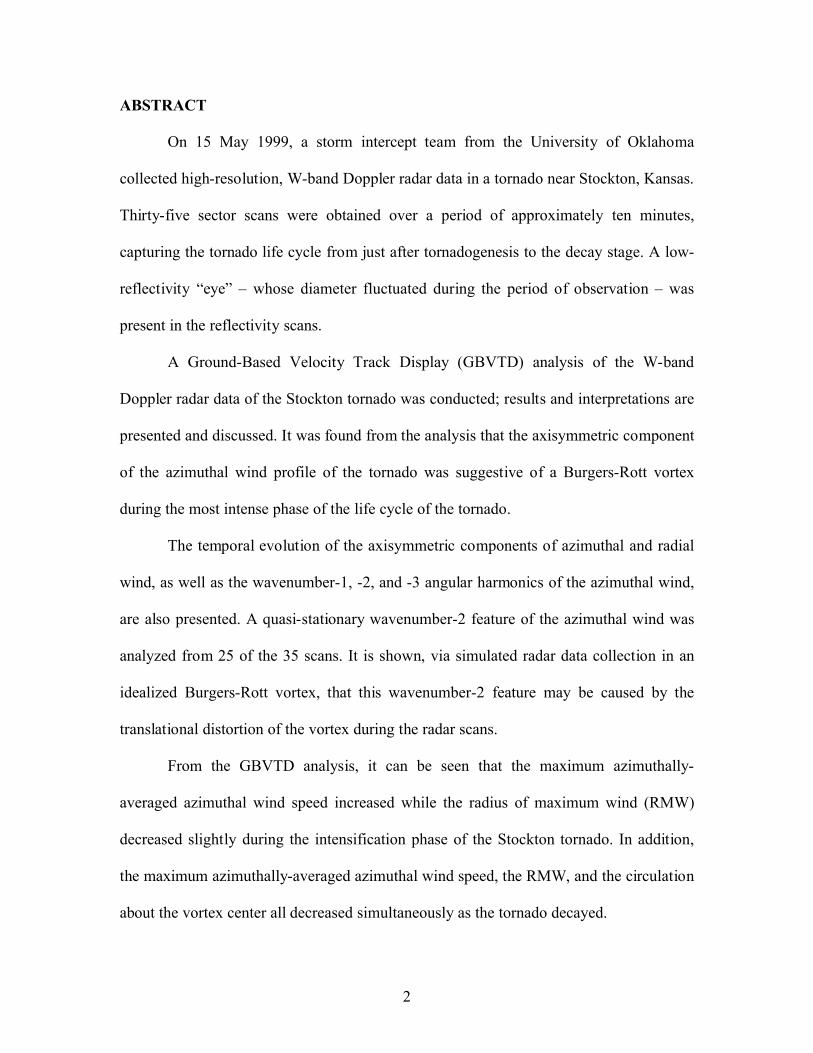
On 15 May 1999, during a University of Oklahoma (OU) School of Meteorology
storm intercept mission, a University of Massachusetts 95-GHz (W-band) mobile
Doppler radar collected high-resolution radar reflectivity and velocity data from several
seconds after tornadogenesis until the end of the life of a tornado that occurred near the
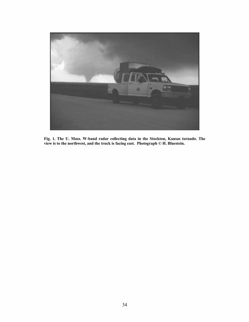
town of Stockton in northwest Kansas (hereafter “the Stockton tornado,” see Fig. 1).
The Stockton tornado occurred in an isolated thunderstorm that developed over
Rooks County, Kansas at around 19:20 CDT. Surface outflow from nearby thunderstorms
6
generated easterly surface flow of 9 m s-1 at a location 18 km south of Stockton
(Bluestein and Pazmany 2000). Aloft, the 00 UTC, 16 May initialization of the Eta model
indicated that southwesterly winds of approximately 18 and 19 m s-1 were present at 500
hPa and 300 hPa, respectively, resulting in a value of shear close to 25 m s-1 between the
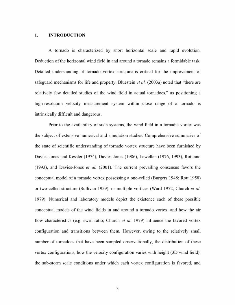
surface and 500 hPa. At the time of the Stockton tornado, the storm appeared as a
somewhat linear reflectivity echo on the Hastings, Nebraska WSR-88D (Fig. 2).
Tornadogenesis occurred around 19:55:12 CDT. During the organizing stage of
the life cycle of the tornado, which lasted approximately two minutes, the condensation
funnel had a ragged appearance. The tornado exhibited a multiple-vortex structure over a
period of about 75 seconds starting around 19:55:30 CDT. The tornado then changed to a
classic “funnel” shape that was maintained for the next eight minutes (the mature stage).
In the last two minutes (the decaying stage) of its life cycle, the condensation funnel
became thinner and corkscrew-like in appearance, before dissipating altogether at
20:06:07 CDT. In general, no multiple vortices were visible during the mature or
decaying stages of the life cycle of the Stockton tornado. The Stockton tornado received a
rating of F1 on the Fujita scale (Fujita 1981) as a result of damage to farmstead
outbuildings and fences (NCDC 1999). Corroboratively, some tree damage was observed
by the storm intercept team (HB). However, the tornado traversed a relatively rural area,
and therefore the tornado had little opportunity to damage well-built structures.
3. W-BAND DOPPLER RADAR DATA
The Doppler radar data used in this study were collected by a mobile, 3 mm
wavelength, 95 GHz (W-band), pulsed Doppler radar built by the University of
Massachusetts (U. Mass) Microwave Remote Sensing Laboratory (Bluestein et al. 1995;

7
hereafter “the W-band radar”). The W-band radar antenna has a half-power beamwidth of
0.18°, and the transmitter has a selectable pulse length of 15 m or 30 m. The W-band
radar transmitter implements a polarization diversity pulse pair (PDPP) technique
(Doviak and Sirmans 1973) that effectively increases its maximum unambiguous velocity
from ±8 m s-1 to ±79 m s-1 (Pazmany et al. 1999). The W-band radar has been used in
numerous severe weather intercept programs (Bluestein et al. 1995, 1997, 2003a, 2003b,
2004b; Pazmany et al. 1999; Bluestein and Pazmany 2000), and has also been used to
collect data on other non-severe meteorological phenomena such as dust devils (Bluestein
et al. 2004a) and drylines (Weiss et al. 2005).
The W-band radar collected thirty-five high-resolution radar reflectivity and
velocity scans in the Stockton tornado (Fig. 1). The first scan was collected at 19:56:19
CDT, and the final scan at 20:06:07 CDT. The time interval between scans was
approximately 15 seconds, except for an interval of approximately one minute (20:01:55
– 20:03:01 CDT) in which no scans were collected. The pulse length of the W-band radar
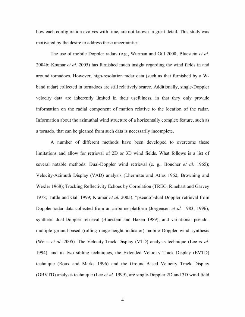
was set to 30 m. The W-band radar was stationary throughout the collection period,
during which the distance to the tornado, which moved towards the north-northwest,
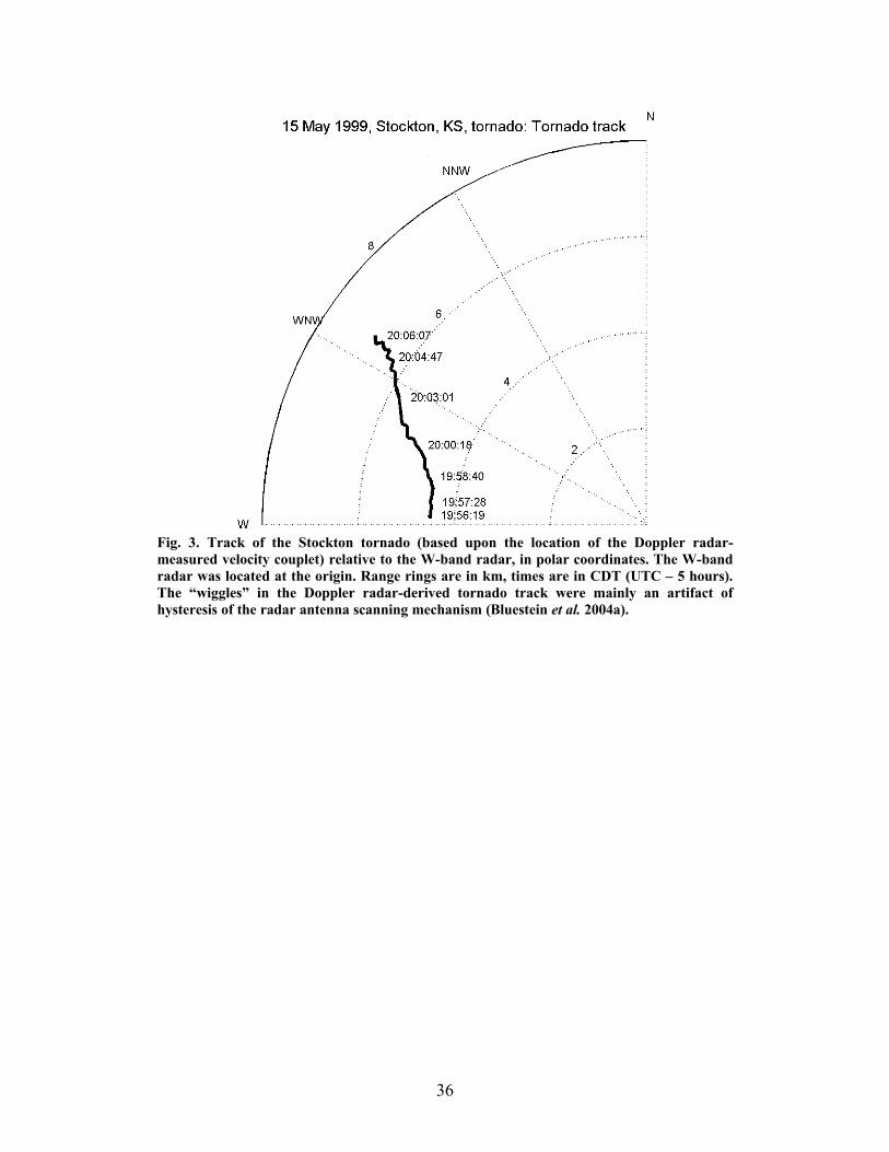
increased from 4.5 km to 6.8 km (Fig. 3).
Significant changes in the structure of the Stockton tornado at various stages of its
life cycle could be inferred from the radar data. Throughout the duration of the
deployment, the tornado was characterized by one or more annuli of relatively high
reflectivity, and was connected to the parent storm by a “thin band” of high reflectivity
(described as an “umbilical cord” by Bluestein and Pazmany [2000]) that was likely a
rain curtain (Fig. 4). In the first 11 scans (covering the time interval from 19:56:19 to

8
19:58:26 CDT), the tornado was characterized by an annulus of relatively high
reflectivity (4 to 8 dBZe) around its center, and possibly a second annulus of moderate
reflectivity (-10 to -5 dBZe) surrounding the inner high-reflectivity annulus (Fig. 4a). In
the 12 scans, covering the time interval from 20:00:55 to 20:05:03 CDT, the tornado was
characterized by a double annulus of relatively high reflectivity (-5 to -1 dBZe, Fig. 4b).
During the time interval between these two groups of scans, the reflectivity structure of
the tornado underwent a transition that can be described as “unraveling”: high-reflectivity
filaments departed the inner high-reflectivity annulus, moved radially outward away from
the center of the vortex, and formed a second, outer high-reflectivity annulus (Fig. 5).
The low-reflectivity “eye” in the center of the tornado, probably formed by the
centrifuging of scatterers outward from the vortex center at, above, and below (assuming
scatterer lofting) the level of the radar scan (Dowell et al. 2005), also exhibited
significant variations in reflectivity structure throughout the course of the data collection.
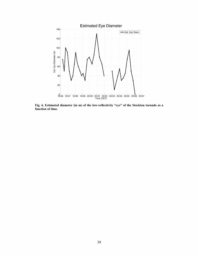
The eye underwent several “pulses” in which its width, as measured by the diametric
distance between maximum negative gradients of reflectivity near the vortex center,
increased and decreased in an arrhythmic fashion (Fig. 6).
During the data collection in the Stockton tornado, the Ford F350 pickup truck
upon which the W-band radar was mounted was not exactly level with respect to the level
ground. As a result, the elevation angle measurements taken with the data were measured
relative to the plane of the truck bed and not that of the level ground. The angle of the
truck bed relative to the plane of the level ground along the line-of-sight between the
truck and the tornado was not accurately known, but has been estimated to be 1.1° ± 0.3°
based upon photogrammetric analysis (described below). (In later seasons, hydraulic
9
levelers were installed on the vehicle, enabling the radar to operate from a level truck bed
and record accurate elevation angles.)
Additionally, the boresighted video camera installed on the radar dish, which is
used by the radar operator to aim the radar beam, provided video feed to the radar
operator, but this video feed was not recorded because the video cassette recorder
malfunctioned. The radar operator indicated that he attempted to aim the radar beam
approximately halfway between the cloud base and the ground as seen in the video feed.
A continuous, time-stamped video recording was obtained of the W-band radar
deployment and the tornado from a location approximately 30 m from the W-band radar
deployment site. A photogrammetric analysis of still 35 mm slides (e.g., Fig. 1) that were
matched to frames in the video, yielded an estimated scan height of 90 m ± 20 m at a
range of 4.5 km from the radar truck, and 125 m ± 30 m at a range of 6.2 km (Fig. 7).
These estimated heights correspond to an estimated radar elevation angle (with respect to
the ground) of 1.1° ± 0.3°. The plane of the radar scan can therefore be assumed to be
quasi-horizontal and the vertical component of motion contained within the measured
along-beam component of the Doppler velocity is insignificant in comparison with the
horizontal component.
4. GBVTD ANALYSIS PROCEDURE
The quasi-axisymmetric structure of the Stockton tornado at the level of the radar
scan made the collected W-band radar dataset a prime candidate for application of
GBVTD analysis. The reader is referred to Lee et al. (1999) and Bluestein et al. (2003b)
for discussions of the GBVTD analysis technique and its application to another case in
which high-resolution W-band radar data was collected in a tornado, respectively. The
10
purpose of applying GBVTD analysis to this radar dataset was twofold: (1) to compare
this case with a previous, similar case (the Bassett, Nebraska tornado of 5 June 1999;
detailed in Bluestein et al. [2003b]), and (2) to ascertain new information about the
structure of a tornado and its variations with time. The GBVTD analysis technique has
been applied to radar data in order to ascertain information about the kinematic structure
of tropical cyclones (Lee et al. 2000), in addition to tornadic vortices (Bluestein et al.
2003b; and the Mulhall tornado of 3 May 1999, discussed in Lee and Wurman [2005]).
Some pre-processing of the W-band radar data was required in order to facilitate
the application of the GBVTD analysis technique. The low-reflectivity eye often
contained relatively noisy velocity data because there were relatively few scatterers
located within. The GBVTD analysis, particularly the simplex center-seeking algorithm
that is used, is somewhat sensitive to erroneous Doppler velocity data. In order to reduce
the effects of such data on the GBVTD analysis, a reflectivity threshold was applied to
the velocity data, using National Center for Atmospheric Research SOLO II radar data
processing software (Oye et al. 1995). Any velocity data point associated with a
reflectivity data point recorded as -18 dBZe or less was ignored; the velocity data from
such points was considered suspect. A few additional velocity data points that were
subjectively judged to be “suspect” (i.e. recorded rays in which the radar beam seemed to
be blocked by a utility pole or other stationary obstruction) were also manually removed.
Successful application of the GBVTD technique requires that the aspect ratio
between the radius of the tornado and the distance from the radar to the tornado not be
excessively large, i.e., that the vortex not be located so close to the radar that the Doppler
signature of the tornado becomes too distorted for accurate analysis (Wood and Brown

11
1992, 1997). The characteristics of the W-band radar dataset collected in the Stockton
tornado satisfied the requirement that the aspect ratio was small, and that the data
locations in radial and azimuthal space could be approximated as a Cartesian grid (Lee et
al. 1999; Bluestein et al. 2003b).
Analysis of the 15 June 1999 Stockton, Kansas tornado radar dataset using the
GBVTD technique involved three main procedures:
1. The reflectivity and velocity data from each of the thirty-five sector scans were
objectively analyzed, using a bilinear interpolation scheme (Mohr et al. 1986),
from their recorded plan position indicator (PPI) grid in radar-centered polar
coordinates (degrees and kilometers) to a constant altitude PPI (CAPPI) Cartesian
coordinate grid with a grid spacing of 20 m. (The change in scan level height with
distance, with respect to the ground, over the 150-m diameter of the tornado,
which was approximately 4 m, was neglected.) The 20 m grid spacing was
selected as a compromise between the radial resolution of the W-band radar (30
m) and its azimuthal resolution (15 m – 20 m) at the range of the Stockton tornado
(4.5 – 6.2 km).
2. The CAPPI grid point nearest the center of the tornado vortex was computed
using the simplex vortex center-seeking algorithm of Lee and Marks (2000). This
objectively determined vortex center was regarded with a high degree of
confidence owing to the results of a sensitivity study (not shown) after that
described in Bluestein et al. (2003b), which indicated that a vortex center
displacement of two grid points or more would likely produce a prominent,
spurious wavenumber-1 component.

12
3. The winds around the vortex center (determined in the previous step) were
computed using the ground-based velocity-track display (GBVTD) analysis
technique.
In the final procedure, the radar data were also transferred into a vortex-centered
coordinate system, and the azimuthal winds were decomposed into azimuthally-averaged
wavenumber-0, -1, -2, and -3 angular harmonic components, as well as wavenumber-0
radial wind components, in 14 concentric annuli of 20 m thickness around the vortex
center.
5. RESULTS
The application of the GBVTD technique to the data collected by the U. Mass W-
band radar yielded a set of GBVTD analyses of the vortex-centered two-dimensional
wind field output for all 35 sector scans Azimuthally-averaged radial profiles of
azimuthal and radial wind were used to calculate azimuthally-averaged horizontal
divergence and vertical vorticity. Azimuthally-averaged values of reflectivity were also
computed. Examples of these analyses that are representative of different stages in the
life cycle of the tornado are shown in Fig. 8. In general, the azimuthally-averaged
azimuthal velocity varied with radius like a Burgers-Rott vortex (BRV; Burgers 1948,
Rott 1958), a version of the Rankine vortex in which the transition from the solid-body
rotation in the inner radii to the potential flow at outer radii is smooth, rather than sharp
or cusp-like. The maximum GBVTD-analyzed azimuthally-averaged azimuthal wind was
45 m s-1, which occurred at 20:03:01 CDT. While this velocity is in the F2 range, it does
not necessarily contradict the F1 rating assigned by NCDC to the Stockton tornado,

13
because the radar data were collected at an altitude on the order of 100 m AGL. In
general, the circulation increased with radius outward from the center of the vortex. The
vorticity near the vortex center was approximately 2 s-1[RB1], which is reasonable for a
tornado.
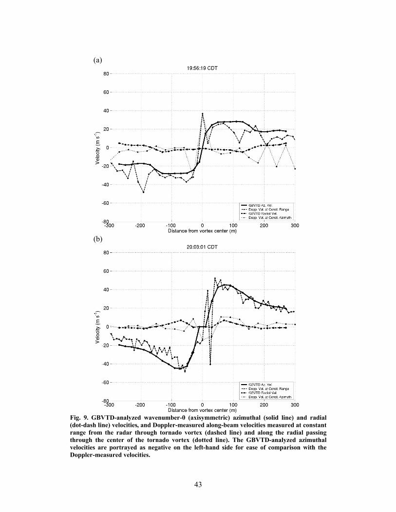
To evaluate the quality of the GBVTD-analyzed azimuthally-averaged azimuthal
(radial) velocities, these velocities were compared to the Doppler velocities measured at a
ring of constant radius from the radar (beam of constant azimuth) passing through the
center of the tornado (e.g., Fig. 9). When the inherent noisiness of the radar data was
taken into account, the sets of curves showed good agreement, and provided confidence
in the results of the GBVTD analysis.
The intensity of the tornado, as measured by the maximum azimuthally-averaged
azimuthal wind speed, reached a peak of 45 m s-1 in the scan taken at 20:03:01 CDT (Fig.
8e). At this time, the radial profile of azimuthally-averaged azimuthal velocity for this
scan bore a strong resemblance to a BRV. Manual fitting of a BRV profile (e.g., Davies-
Jones 1983) to the maximum wind value and radius of maximum wind (RMW) only
(45.0 m s-1 at 70 m) yields the agreeable profile shown in Fig. 10b. The profile
underestimates the velocities beyond the RMW, indicating that perhaps the circulation is
being underestimated in the BRV model.
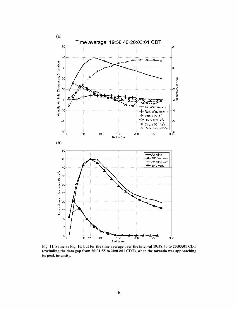
A number of prominent features emerged from the time-averaged radial profiles
of azimuthal and radial velocity, vorticity, divergence, and reflectivity during the time
interval in which the tornado was approaching its peak intensity (19:58:40 to 20:03:01
CDT; Fig. 11). First, the RMW was located outside of the radius of maximum reflectivity
(RMR), indicating that the highest velocities were located outside of the range ring with

14
the greatest numbers of scatterers. Bluestein et al. (2004a) noted the same pattern in some
W-band radar scans of dust devils in Texas, and hypothesized that it resulted from small
particles being concentrated in the center of the vortex as a result of a frictionally induced
surface layer inflow. Second, the radial profile of azimuthally-averaged radial velocity in
the vortex at the level of the radar scan resembled that of a two-celled vortex (Sullivan
1959), although this structure cannot be definitively diagnosed via GBVTD analysis
owing to uncertainties in the analyzed radial velocity, particularly at very small radii.
Assuming that the two-celled vortex model was applicable and mass continuity was valid
at the level of the radar scan, divergence (and possibly sinking motion aloft) was
indicated between 30 – 140 m from the vortex center (a span encompassing the RMW),
while convergence (and possibly rising motion aloft) was indicated between 140 m and
260 m (well outside of the RMW). Dowell et al. (2005) assert that the velocities of
centrifuged scatterers within a tornado may not be indicative of actual wind speeds inside
of the tornado; however, this potential source of radial velocity (and hence, divergence)
measurement error applies mainly to Doppler radar scans containing significant quantities
of large scatterers, which were probably not present at the level of the radar scan (90 –
150 m AGL) in the Stockton tornado, except during intermittent periods. Third, the time-
averaged radial profile of azimuthally-averaged azimuthal wind again resembles a BRV.
After the scan in which the tornado reached its peak intensity (20:03:01 CDT), the
azimuthally-averaged azimuthal wind quickly decreased over the next three minutes as
the tornado dissipated.
6. INTERPRETATION OF THE DATA

15
Fig. 12 (Fig. 13) depicts the evolution of the azimuthally-averaged azimuthal
wind (circulation) structure as a function of time and radius. The maximum azimuthally-
averaged (wavenumber-0) component of the azimuthal wind increased in magnitude as
the tornado progressed through its life cycle, and displayed good temporal continuity
until the tornado began to decay around 20:04:00 CDT. The circulation around the
tornado increased from approximately 5,000 m2 s-1 at the innermost analyzed radii to
between 30,000 – 45,000 m2 s-1 at outermost analyzed radii when the tornado was in its
mature stage. The decay phase of the Stockton tornado’s life cycle is indicated both by a
decrease in the maximum azimuthally-averaged azimuthal wind and a decrease in
circulation of the wavenumber-0 component of the azimuthal wind at all radii (Fig. 13).
The azimuthally-averaged radial wind component of the tornado displayed a
temporally coherent period of maximum velocity (6 – 10 m s-1 away from the vortex
center) at roughly the same radii (60 – 120 m) and times (19:58:40 – 20:03:01 CDT) that
the tornado was approaching its peak intensity (Fig. 14). Inflow into the tornado, manifest
as outbound velocities at the height of the scan at these radii and times, is consistent with
the two-celled vortex model; however, as noted previously, a two-celled structure cannot
be definitively diagnosed using this analysis. The GBVTD-analyzed values of
azimuthally-averaged radial velocity at radii less than 40 m should be considered
particularly suspect because relatively few velocity data points contributed to the
GBVTD analysis.
The GBVTD analyses also yielded azimuthally-averaged radial profiles of higher
order angular harmonics of the azimuthal wind (wavenumbers-1, -2, and -3). All three of
these components (not shown) display poor temporal continuity and are of little value for

16
interpretation. However, a relatively strong wavenumber-2 component of azimuthal
velocity, manifest as two quasi-diametrically opposed “lobes” of relatively high values of
analyzed azimuthal velocity (e.g. Fig. 8c, e), was visibly present in 25 of the 35 analyses,
with a wavenumber-2 magnitude of or exceeding 5 m s-1.
Previous GBVTD analyses of radar data collected in tornadoes also exhibited a
prominent wavenumber-2 component (Bluestein et al. 2003b; Lee and Wurman 2005).
The reason for this feature is not definitively determined. It has been suggested that the
wavenumber-2 component may be an artifact of the GBVTD analysis, or may in fact be a
physical feature associated with tornadoes (Bluestein et al. 2003b). The orientation of the
wavenumber-2 feature does not appear to be correlated with the direction of the radar
beam, nor does it exhibit continuity in magnitude or orientation from scan to scan. It is
also unlikely that the wavenumber-2 feature is the result of aliasing from higher-order
harmonics (wavenumber-4, wavenumber-6, etc.) owing to the relatively small
contribution to the total azimuthal velocity component from the latter (Fig. 15).
A possible physical explanation for the wavenumber-2 feature is that it is a result
of elliptical asymmetry of the vortex caused by translational and frictional effects
(Shapiro 1983). Lee et al. (2005) hypothesized that a wavenumber-2 vortex Rossby wave
(e.g., Montgomery and Kallenbach 1997) may actually be present in elliptically-shaped
atmospheric vortices, but one would expect the high-velocity “lobes” to revolve around
the center of the tornado (Bluestein et al. 2003b), and this progression is not obvious in
the analyses. The presence of a wavenumber-2 vortex Rossby wave would be impossible
to verify without high-resolution volumetric radar data collected in close proximity to the
vortex.

17
The authors believe that a likely explanation for the wavenumber-2 feature is that
it is an artifact resulting from the motion of the tornado during the time interval over
which a radar scan was collected. The motion of the vortex (approximately 7 m s-1 to the
north-northwest) during the time interval required to collect the radar scan
(approximately 10 s) is enough to distort the vortex into an ellipse. The distortion of the
vortex causes a spurious wavenumber-2 feature in the resulting GBVTD analysis.
In idealized experiments, a BRV azimuthal velocity profile closely resembling
that of a tornado was sought. Subjectively-guessed values of circulation Γ (45,000 m2 s-
1), RMW (70 m), and azimuthal velocity at the RMW (80 m s-1) were used. An idealized,
cyclonic vortex with this velocity profile, centered at the point (0 m, 5000 m), was
generated. This vortex velocity field was “sampled” with a radial resolution of 10 m and
an azimuthal resolution of 0.2° (mimicking somewhat the 30 m radial resolution and
0.18° beamwidth of the W-band radar) by a stationary “radar” located at the origin. The
along-beam component of vortex velocity was calculated, and an instantaneous simulated
Doppler velocity field (not shown) was generated.
This procedure was repeated, this time simulating the Doppler velocity field that
would be generated by a Doppler radar scanning a horizontally-translating BRV with the
same velocity field. Doppler velocity scans were simulated for combinations of three
different antenna rotation rates (+1, +2, and +4° s-1), four vortex translation speeds (0, 5,
10, and 15 m s-1), and eight different directions of motion (0 - 315° in increments of 45°).
The simulated Doppler velocity fields were then interpolated to a Cartesian grid with a
resolution of 20 m, and subjected to velocity track display (VTD, Lee et al. 1999)
analysis about the vortex center.

18
It was observed that a wavenumber-2 component (with varying degrees of
prominence) was analyzed from most of these simulated Doppler radar scans (not
shown). In order to see how well the simulation matched up with the analysis results, an
additional simulation was conducted in which the simulated BRV closely mimicked the
characteristics (RMW, maximum azimuthal velocity, position, and motion) of the tornado
at 20:03:01 CDT. The simulated radar data were generated using nearly the same
“scanning” strategy (antenna rotation rate and direction) as that of the actual W-band
radar. The resulting GBVTD analysis is shown in Fig. 16. This analysis features a
prominent wavenumber-2 component with an amplitude of 5 m s-1 (relative to
wavenumber-0 component of 40 m s-1) at a radius of 70 m from the center of the vortex.
Although the orientation of the wavenumber-2 features differ, the structural similarities
between Fig. 8e and Fig. 16 are remarkable. These results lead the authors to favor vortex
transation as an explanation of the wavenumber-2 feature.
A possible explanation for the poor temporal continuity in orientation of the
wavenumber-2 feature is the presence of a vertically-propagating wavenumber-2 feature
(such as an inertial wave) within the tornado vortex structure. However, as with a vortex
Rossby wave, such a feature would be impossible to resolve without rapidly-collected,
high-resolution, volumetric radar data. Another possible explanation is the alternating
azimuthal direction of radar sweep that is responsible for the “wiggles” in the tornado
track (Fig. 3). This apparent change in direction and speed of the tornado can, in turn,
influence the results of the GBVTD analysis.
The observed vortex structure is complex, and any underlying physical
wavenumber-two asymmetry may be distorted by the above mentioned artifacts. In order

19
to further elucidate the physical vortex asymmetries, methods to compensate for
distortion of the vortex and the motion of the radar antenna are currently under
development.
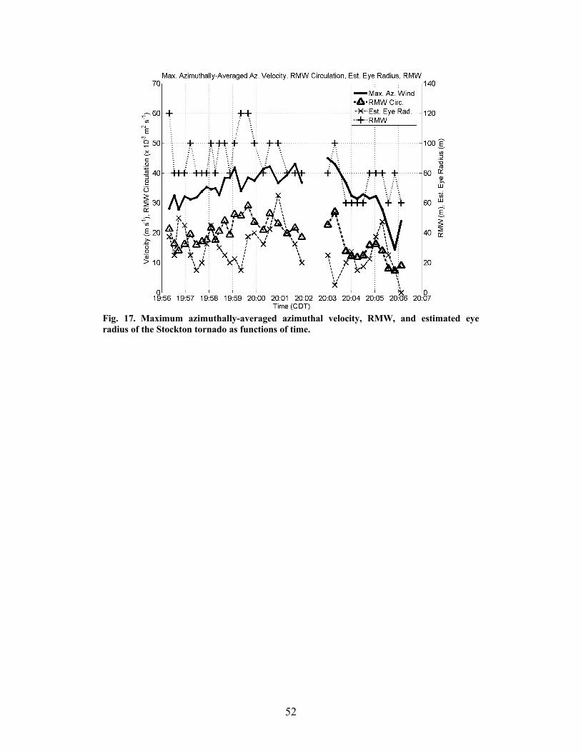
A number of significant features of the evolution of the Stockton tornado became
apparent when several time-dependent variables were plotted on the same axis (Fig. 17).
First, the low-reflectivity eye width decreased as the tornado approached its peak
intensity (as measured by the maximum azimuthally-averaged azimuthal wind) at
20:03:01 CDT, and then increased again as the tornado decayed. This fluctuation in eye
width could be indicative of increased lofting of small raindrops and low-density debris
particles (such as grass and dust) near the RMW as the intensity of the tornado increased
(D. Burgess 2004, personal communication). Dowell et al. (2005), using a quasi-3-D
simulation of an axisymmetric tornadic vortex, showed that relatively small particles
(such as raindrops) can be concentrated near the core of the tornado in the surface inflow
layer, and then transported upward by the central updraft. Other arrhythmic fluctuations
in eye width could result from the intermittent ingestion by the tornado of large quantities
of small particles, which were then lofted to the level of the radar scan (Bluestein et al.
2004a).
Secondly, during the intensification period of the tornado (19:58:40 - 20:03:01
CDT), it can be seen that an increase in the maximum azimuthally-averaged azimuthal
wind at a relatively steady RMW resulted in an increase in circulation at the RMW. This
manner of tornado intensification contrasts with that found by Bluestein et al. (2003b) in
their GBVTD analysis of the 5 June 1999 Bassett, Nebraska tornado (hereafter, “the
Bassett tornado”). The RMW of the Bassett tornado decreased while the maximum

20
azimuthally-averaged azimuthal wind increased, and the circulation of the tornado at the
RMW increased. This result suggests that more than one mode of tornado intensification
exists.
Thirdly, it can be seen that as the tornado decreased in intensity towards the end
of its life cycle (after 20:03:01 CDT), the RMW also generally decreased. This result is
consistent with the visual appearance of the tornado; the visible condensation funnel
appeared to narrow before dissipating. This behavior contrasts markedly with the decay
mode found by Bluestein et al. (2003b) in the Bassett tornado. The Bassett tornado
exhibited an increase in the RMW and a simultaneous decrease in maximum azimuthally-
averaged azimuthal wind. This result suggests that more than one mode of tornado decay
exists, a conclusion that is consistent with the two decay modes suggested by Davies-
Jones et al. (2001).
7. CONCLUSIONS
Application of the GBVTD analysis technique provided insights on the horizontal
wind field in the 15 May 1999 Stockton, Kansas tornado, in which exceptionally high-
quality W-band radar data were collected. From the GBVTD analysis, it can be inferred
that the Stockton tornado wind field at the height of the radar scan resembled that of a
Burgers-Rott vortex during the period in which the tornado approached its peak intensity
(19:58:40 – 20:03:01 CDT).
It can be seen from the radar data that the width of the low-reflectivity “eye” in
the center of the tornado vortex fluctuated from scan to scan. Of particular interest, the
eye width decreased as the tornado approached its peak intensity at 20:03:01 CDT. One
might expect that the width of the eye would increase with increasing tornado intensity as

21
a result of increased centrifuging of scatterers (Dowell et al. 2005). It is noted that the eye
width decreased again as the tornado decayed. These fluctuations could be indicative of
increased ingestion and lofting of light debris inside the tornado, up to the altitude of the
radar scan, as the intensity of the tornado increased.
From a comparison of the GBVTD analyses of the Stockton tornado and the
Bassett tornado (Bluestein et al. 2003b), it can be inferred that tornadoes exhibit two or
more different modes of intensification and two or more different modes of decay. As the
RMW remained relatively constant during the intensification phase of the Stockton
tornado, with a few noticeable exceptions, the increase in RMW circulation resulted
primarily from an increase of the maximum azimuthally-averaged azimuthal velocity; the
RMW circulation in the Bassett tornado increased as a result of an increase of the
maximum azimuthally-averaged velocity that occurred along with a simultaneous
decrease of the RMW. The RMW circulation of the Stockton tornado decayed as a result
of a simultaneous decrease of both the maximum azimuthally-averaged azimuthal
velocity and the RMW; the RMW circulation of the Bassett tornado decayed as a result
of a decrease of the maximum azimuthally-averaged azimuthal velocity, despite an
increase of the RMW.
A significant wavenumber-2 component, with its amplitude at or exceeding 5 m s-
1, of the azimuthal wind was present in 25 out of 35 of the W-band sector scans. Similar
wavenumber-2 features have been observed in previous studies in which the GBVTD
analysis technique has been applied to mobile radar data collected in tornadoes. The
presence of the wavenumber-2 feature in analyses of data collected by multiple radars
(Lee and Wurman 2005; Bluestein et al. 2003b) suggests that the wavenumber-2 feature
22
may have a physical basis. However, it was shown in this study that the wavenumber-2
feature likely resulted from the distortion of the vortex in the radar image caused by the
vortex motion. Methods to compensate for this distortion in the radar data are being
developed and will be the subject of future work.
Additional GBVTD analyses of mobile radar data collected in other tornadoes
could provide a means of strengthening or disproving theories about tornado structure
and evolution presented in this study and elsewhere. GBVTD analyses of data from
radars with higher scan rates than the W-band radar could potentially clarify the source of
the wavenumber-2 feature that has been repeatedly observed in mobile radar data
collected in tornadoes. GBVTD analyses of data from radars that collect data at multiple
elevation angles simultaneously (e.g. the rapid-scan Doppler on Wheels, or DOW5;
Wurman and Randall 2001) and from dual-polarization radars (e. g., Lopez et al. 2004)
could also potentially illuminate the structure of tornadoes.

23
8. ACKNOWLEDGMENTS
This research was conducted as part of the first author’s master’s thesis project.
Dr. Stephan P. Nelson of the National Science Foundation (NSF) supported this research
under NSF grants ATM-9320672, ATM-9616730, ATM-0241037, and supplements to
NSF grants ATM-9019821, ATM-9302379, and ATM-9612674. Dr. David Dowell of the
Cooperative Institute for Mesoscale Meteorological Studies at OU furnished a copy of his
video recording of the Stockton tornado. Dr. Mark Laufersweiler provided technology
support. Dr. Erik Rasmussen provided nowcasting support. Dr. Michael I. Biggerstaff and
Dr. Alan Shapiro of OU, Dr. Louis J. Wicker, Dr. David Jorgensen, Donald W. Burgess
and Vincent T. Wood of the National Severe Storms Laboratory, and Dr. Christopher C.
Weiss of Texas Tech University provided discussion and assistance throughout the
research process. The authors gratefully acknowledge three anonymous reviewers who
helped us to greatly improve the clarity and quality of the manuscript.

24
9. REFERENCES
Bluestein, H. B., and D. S. Hazen, 1989: Doppler-radar analysis of a tropical cyclone
over land: Hurricane Alicia (1983) in Oklahoma. Mon. Wea. Rev., 117, 2594 – 2611.
―――――, and A. L. Pazmany, 2000: Observations of tornadoes and other convective
phenomena with a mobile, 3-mm wavelength, Doppler radar: The spring 1999 Field
Experiment. Bull. Amer. Meteor. Soc., 81, 2939 – 2951.
―――――, ―――――, J. C. Galloway, and R. E. Mcintosh, 1995: Studies of the
substructure of severe convective storms using a mobile 3-mm-wavelength Doppler
radar. Bull. Amer. Meteor. Soc.. 76, 2155 – 2170.
―――――, S. G. Gaddy, D. C. Dowell, A. L. Pazmany, J. C. Galloway, R. E. McIntosh
and H. Stein, 1997: Doppler radar observations of substorm-scale vortices in a
supercell. Mon. Wea. Rev., 125, 1046 – 1059.
―――――, C. C. Weiss, and A. L. Pazmany, 2003a: Mobile Doppler radar observations
of a tornado in a supercell near Bassett, Nebraska, on 5 June 1999. Part I:
Tornadogenesis. Mon. Wea. Rev., 131, 2954 – 2967.
―――――, W.-C. Lee, M. Bell, C. C. Weiss, and A. L. Pazmany, 2003b: Mobile
Doppler radar observations of a tornado in a supercell near Bassett, Nebraska, on 5
June 1999. Part II: Tornado-vortex structure. Mon. Wea. Rev., 131, 2968 – 2984.
―――――, C. C. Weiss and A. L. Pazmany, 2004a: Doppler radar observations of dust
devils in Texas. Mon. Wea. Rev., 132, 209 – 224.
―――――, ――――― and ―――――, 2004b: The vertical structure of a tornado
near Happy, Texas, on 5 May 2002: High-resolution, mobile, W-band, Doppler radar
observations. Mon. Wea. Rev., 132, 2325 – 2337.
25
Boucher, R. J., R. Wexler, D. Atlas, and R. M. Lhermitte, 1965: Mesoscale structure
revealed by Doppler radar. J. Appl. Meteor., 4, 590 – 597.
Browning, K.A., and R. Wexler, 1968: The determination of kinematic properties of a
wind field using Doppler radar. J. Appl. Meteor., 7, 105 – 113.
Burgers, J. M., 1948: A mathermatical model illustrating the theory of turbulence. Adv.
Appl. Mech., 1, 197 – 199.
Church, C. R., J. T. Snow, G. L. Baker, and E. M. Agee, 1979. Characteristics of tornado-
like vortices as a function of swirl ratio: A laboratory investigation. J. Atmos. Sci., 36,
1755 – 1776.
Davies-Jones, R., 1986: Tornado dynamics. Thunderstorm Morphology and Dynamics.
2d ed. E. Kessler (Ed.), University of Oklahoma Press, 197 - 236.
―――――, and E. Kessler, 1974: Tornadoes. Weather and Climate Modification, W. N.
Hess (Ed.), Wiley and Sons, 552 – 595.
―――――, R. J. Trapp, and H. B. Bluestein, 2001: Tornadoes and tornadic storms.
Severe Convective Storms. C. A. Doswell III (Ed.), Meteor. Monogr., No. 28, Amer.
Meteor. Soc., 167 – 221.
Doviak, R. J., and D. Sirmans, 1973. Doppler radar with polarization diversity. J. Atm.
Sci., 30, 737 – 738.
Dowell, D. C., and H. B. Bluestein, 2002: The 8 June 1995 McLean, Texas, storm. Part I:
Observations of cyclic tornadogenesis. Mon. Wea. Rev., 130, 2626 – 2648.
―――――, C. A. Alexander, J. Wurman, and L. J. Wicker, 2005: Centrifuging of
hydrometeors and debris in tornadoes: Radar-reflectivity patterns and wind-
measurement errors. Mon. Wea. Rev., 133, 1501 – 1524.

26
Fujita, T. T., 1981: Tornadoes and downbursts in the context of generalized planetary
scales. J. Atmos. Sci., 38, 1511 – 1534.
Jorgensen, D. P., P. H. Hildebrand, and C. L. Frush, 1983: Feasibility test of an airborne
pulse-Doppler meteorological radar. J. Appl. Meteor., 22, 744 – 757.
―――――, T. Matejka, and J. D. DuGranrut, 1996: Multi-beam techniques for deriving
wind fields from airborne Doppler radars. J. Meteor. Atmos. Phys., 59, 83 – 104.
Kramar, M. R., H. B. Bluestein, A. L. Pazmany, and J. D. Tuttle, 2005: The “Owl Horn”
radar signature in developing Southern Plains supercells. Mon. Wea. Rev. (In press.)
Lee, W.C., and F. D. Marks Jr., 2000. Tropical cyclone kinematic structure retrieved
from single-Doppler radar observations. Part II: The GBVTD-Simplex center-finding
algorithm. Mon. Wea. Rev., 128, 1925 – 1936.
―――――, and J. Wurman, 2005: Diagnosis of 3D wind structure of the Mulhall,
Oklahoma tornado of 3 May 1999. J. Atmos. Sci., 62, 2373 – 2393.
―――――, F. D. Marks Jr., and R. E. Carbone, 1994: Velocity track display – A
technique to extract real-time tropical cyclone circulations using a single airborne
Doppler radar. J. Atmos. Oceanic Technol., 11, 337 – 356.
―――――, B. J.-D. Jou, P.-L. Chang, and S.-M. Deng, 1999: Tropical cyclone
kinematic structure retrieved from single-Doppler radar observations. Part I: Doppler
velocity patterns and the GBVTD technique. Mon. Wea. Rev., 127, 2419 – 2439.
―――――, B. J-.D. Jou, P.-L. Chang, and F. D. Marks Jr., 2000. Tropical cyclone
kinematic structure retrieved from single-Doppler radar observations. Part III:
Evolution and structures of Typhoon Alex. Mon. Wea. Rev., 128, 3982 – 4001.

27
―――――, P. Harasti, M. Bell, B. J.-D. Jou, H.-H. Chang, 2005: Doppler velocity
signatures of idealized elliptical vortices. Accepted, Terretrial, Atmospheric, and
Oceanic Sciences (Taiwan).
Lewellen, W. S., 1976: Theoretical models of the tornado vortex. Proceedings,
Symposium on Tornadoes: Assessment of Knowledge and Implications for Man, R. E.
Peterson (Ed.), Texas Tech University, 107 – 143.
―――――, 1993: Tornado vortex theory. The Tornado: Its Structure, Dynamics,
Prediction, and Hazards, Geophys. Monogr., No. 79, Amer. Geophys. Union, 19 –
39.
Lhermitte, R. M., and D. Atlas, 1962: Precipitation motion by pulse Doppler radar. Proc.
Ninth Weather Radar Conf., Kansas City, MO, Amer. Meteor. Soc., 218-223.
Lopez, F. J., A. L. Pazmany, H. B. Bluestein, M. R. Kramar, M. F. French, C. C. Weiss,
and S. Frasier, 2004: Dual-polarization, X-band, mobile Doppler radar observations
of hook echoes in supercells. Preprints, 22nd Conf. on Severe Local Storms, Hyannis,
MA, Amer. Meteor. Soc., CD-ROM, P11.7.
Mohr, C. G., L. J. Miller, R. L. Vaughn, and H. W. Frank, 1986: Merger of mesoscale
dataset into a common Cartesian format for efficient and systematic analysis. J.
Atmos. Oceanic Technol., 3, 143 – 161.
Montgomery, M. T., and R. J. Kallenbach, 1997: A theory for vortex Rossby-waves and
its application to spiral bands and intensity changes in hurricanes. Quart. J. Roy.
Meteor. Soc., 123, 435–465.
NCDC, 1999: Storm Data. Vol. 37, No. 5, 372 pp. [Available online at
http://www5.ncdc.noaa.gov/pubs/publications.html.]
28
Oye, R. C. K. Mueller, and S. Smith, 1995: Software for radar translation, editing, and
interpolation. Preprints, 27th Conf. on Radar Meteorology, Amer. Meteor. Soc., 359 –
361.
Pazmany, A. L., J. C. Galloway, J. B. Mead, I. Popstefanija, R. E. McIntosh and H.
B. Bluestein, 1999: Polarization diversity pulse-pair technique for millimeter-wave
Doppler radar measurements of severe storm features. J. Atmos. Oceanic Technol.,
16, 1900 – 1911.
Rinehart, R. E., and E. T. Garvey, 1978: Three-dimensional storm motion detection by
conventional weather radar. Nature, 273, 287-289.
Rott, N., 1958: On the viscous core of a line vortex. Z. Angew. Math. Phys., 9, 543-553.
Rotunno, R., 1993: Supercell thunderstorm modeling and theory. The Tornado: Its
Structure, Dynamics, Prediction, and Hazards, Geophys. Monogr., No. 79, Amer.
Geophys. Union, 57 – 73.
Roux, F., and F. D. Marks, Jr., 1996: Extended Velocity Track Display (EVTD): An
improved processing method for Doppler radar observations of tropical cyclones. J.
Atmos. Oceanic Technol., 13, 875 – 899.
Shapiro, L. J., 1983: The asymmetric boundary flow layer under a translating hurricane.
J. Atmos. Sci., 40, 1984 – 1998.
Sullivan, R. D., 1959: A two-cell vortex solution of the Navier-Stokes equations. J.
Aerospace Sci., 26, 767-768.
Tuttle, J., and R. Gall, 1999: A single-radar technique for estimating the winds in tropical
cyclones. Bull. Amer. Meteor. Soc., 80, 653 – 668.
29
Wakimoto R. M., and H. Cai, 2000: Analysis of a nontornadic storm during VORTEX
95. Mon. Wea. Rev., 128, 565 – 592.
―――――, R. M., C. Liu and H. Cai, 1998: The Garden City, Kansas, storm during
VORTEX 95. Part I: Overview of the storm’s life cycle and mesocyclogenesis. Mon.
Wea. Rev., 126, 372 – 392.
―――――, R. M., H. V. Murphey, D. C. Dowell and H. B. Bluestein, 2003: The
Kellerville tornado during VORTEX: Damage survey and Doppler radar analyses.
Mon. Wea. Rev., 131, 2197 – 2221.
Ward, N. B., 1972: The exploration of certain features of tornado dynamics using a
laboratory model. J. Atmos. Sci., 29, 1194–1204.
Weiss, C. C., H. B. Bluestein and A. L. Pazmany, 2005: Fine-scale radar
observations of the 22 May 2002 dryline during the International H2O
Project (IHOP). (accepted, Mon. Wea. Rev.)
Wood, V. T., and R. A. Brown, 1992: Effects on radar proximity on single-Doppler
velocity signatures of axisymmetric rotation and divergence. Mon. Wea. Rev., 120,
2798-2807.
―――――, and ―――――, 1997: Effects of radar sampling on single-Doppler
velocity signatures of mesocyclones and tornadoes. Wea. Forecasting, 12, 928 – 938.
Wurman, J., and S. Gill, 2000: Finescale radar observations of the Dimmitt, Texas (2
June 1995), tornado. Mon. Wea. Rev., 128, 2135 – 2164.
―――――, and M. Randall, 2001: An inexpensive, mobile, rapid-scan radar. Preprints,
30th Conf. on Radar Meteorology, Munich, Germany, Amer. Meteor. Soc., CD-ROM,
P3.4.
30
10. FIGURES
Fig. 1. The U. Mass. W-band radar collecting data in the Stockton, Kansas tornado. The
view is to the northwest, and the truck is facing east. Photograph © H. Bluestein.
Fig. 2. WSR-88D reflectivity image of the storm that produced the Stockton tornado,
taken at 19:59 CDT by the WSR-88D located at Hastings, Nebraska (KUEX). The
range rings are spaced at 50 km intervals, and the azimuthal spacing is 30°. The
black square indicates the approximate location of the U. Mass. W-band radar; the
inverted triangle indicates the approximate location of the tornado. The motion of
the storm was towards the northeast.
Fig. 3. Track of the Stockton tornado (based upon the location of the Doppler radar-
measured velocity couplet) relative to the W-band radar, in polar coordinates. The
W-band radar was located at the origin. Range rings are in km, times are in CDT
(UTC – 5 hours). The “wiggles” in the Doppler radar-derived tornado track were
mainly an artifact of hysteresis of the radar antenna scanning mechanism (Bluestein
et al. 2004a).
Fig. 4. W-band reflectivity in dBZe (top) and Doppler velocity in m s-1 (bottom) in the
Stockton tornado at (a) 19:56:19 CDT and (b) 20:03:01 CDT. The azimuthal grid
spacing is 1° and the radial grid spacing is 0.1 km. The black arrows indicate the
location of the thin band of relatively high reflectivity connecting the vortex to the
parent storm. The orientation of north is towards the top of the page.
Fig. 5. Sequence of W-band reflectivity images from (a) 19:59:55, (b) 20:00:18, (c)
20:00:34, and (d) 20:00:55 CDT, showing the formation of the outer high-
reflectivity annulus from the “unraveling” of an inner one (indicated by arrows).

31
Note also the temporal continuity of the thin band of high reflectivity at right
connecting the vortex to its parent storm. The azimuthal grid spacing is 1° and the
radial grid spacing is 0.1 km. The orientation of north is toward the top of the page.
Fig. 6. Estimated diameter (in m) of the low-reflectivity “eye” of the Stockton tornado as
a function of time.
Fig. 7. Photogrammetric analyses of still photographs, obtained using a camera with a
known focal length, that were matched to video frames (not shown). Photographs ©
H. Bluestein.
Fig. 8. (Left column) Reflectivity (filled gray contours with intervals of 5 dBZe) and
GBVTD-analyzed azimuthal velocity (sum of wavenumbers 0 through 3, in contour
intervals of 10 m s-1). The direction of the radar beam is indicated by the arrow.
(Right column) Radial profile of GBVTD-analyzed azimuthally-averaged azimuthal
velocity (m s-1), radial velocity (m s-1), vorticity (s-1 x 10), divergence (s-1 x 100),
circulation (m2 s-1 x 10⁻³), and reflecitivity (dBZe). Positive radial velocity indicates
flow away from the tornado vortex center. These analyses were performed for the
W-band radar scans collected at (a, b) 19:59:19 CDT, just after tornadogenesis; (c,
d) 19:59:05 CDT, as the intensity of the tornado increased; (e, f) 20:03:01 CDT,
when the tornado attained its peak intensity; and (g, h) 20:06:07 CDT, when the
tornado dissipated.
Fig. 9. GBVTD-analyzed wavenumber-0 (axisymmetric) azimuthal (solid line) and radial
(dot-dash line) velocities, and Doppler-measured along-beam velocities measured at
constant range from the radar through tornado vortex (dashed line) and along the
radial passing through the center of the tornado vortex (dotted line). The GBVTD-

32
analyzed azimuthal velocities are portrayed as negative on the left-hand side for ease
of comparison with the Doppler-measured velocities.
Fig. 10. (a) Radial profile of GBVTD-analyzed azimuthally-averaged azimuthal velocity
(m s-1), radial velocity (m s-1), vorticity (s-1 x 10), divergence (s-1 x 100), circulation
(m2 s-1 x 10⁻³), and reflectivity (dBZe) at 20:03:01 CDT, when the tornado was at
peak intensity. Positive radial velocity indicates flow away from the tornado vortex
center. (b) Radial profile of GBVTD-analyzed azimuthally-averaged azimuthal
velocity from 20:03:01 CDT (solid curve), the azimuthal velocity profile of a BRV
with the same maximum velocity value and RMW (solid curve with triangular
markers). The vorticity associated with each of the profiles (multiplied by a factor of
10 for clarity) is indicated by broken lines with corresponding symbols.
Fig. 11. Same as Fig. 10, but for the time average over the interval 19:58:40 to 20:03:01
CDT (excluding the data gap from 20:01:55 to 20:03:01 CDT), when the tornado
was approaching its peak intensity.
Fig. 12. Hovmøeller diagram of the azimuthally-averaged (wavenumber-0) component of
the azimuthal velocity as a function of radius in the Stockton tornado, as computed
by the GBVTD analysis. The radius of the eye approached 60 m around 20:01 CDT,
resulting in the abnormally small velocities analyzed in the 20-40 m radius ring at
that time. Minimum F0 tornado velocity is 35 m s-1.
Fig. 13. Hovmøeller diagram of azimuthally-averaged circulation as a function of radius
in the Stockton tornado, computed from the GBVTD-analyzed, azimuthally-
averaged wavenumber-0 component of the azimuthal velocity.

33
Fig. 14. Hovmøeller diagram of azimuthally-averaged radial velocity as a function of
radius in the Stockton tornado, as computed by the GBVTD analysis. Note the
coherent interval of inflow between 60 and 120 m radius during the time interval
19:58:40 to 20:03:01 CDT. The analyzed values at 20:04:31 CDT are highly suspect
because the reflectivities in the vortex were relatively small over the entire GBVTD
analysis domain.
Fig. 15. (a, b) Same GBVTD analyses depicted in Fig. 8(a, e, respectively), but with
wavenumber-4 also included. The direction of the radar beam is indicated by the
black arrow. North is towards the top of the page.
Fig. 16. GBVTD-analyzed azimuthal velocity fields (black contours in increments of 5 m
s-1), generated from simulated radar scans in which an idealized BRV translated at
11 m s-1 at an angle of 5° clockwise from north, a motion similar to the tornado
observed at 20:03:01 CDT. For comparison, the idealized BRV azimuthal velocity
field (filled gray contours, scale at bottom) is also shown. The vector pointing from
the “radar” to the simulated vortex center is indicated by the solid black arrow, and
the direction of motion of the vortex by the dashed arrow.
Fig. 17. Maximum azimuthally-averaged azimuthal velocity, RMW, and estimated eye
radius of the Stockton tornado as functions of time.
34
Fig. 1. The U. Mass. W-band radar collecting data in the Stockton, Kansas tornado. The view is to the northwest, and the truck is facing east. Photograph © H. Bluestein.

35
Fig. 2. WSR-88D reflectivity image of the storm that produced the Stockton tornado, taken at 19:59 CDT by the WSR-88D located at Hastings, Nebraska (KUEX). The range rings are spaced at 50 km intervals, and the azimuthal spacing is 30°. The black square indicates the approximate location of the U. Mass. W-band radar; the inverted triangle indicates the approximate location of the tornado. The motion of the storm was towards the northeast.
36
Fig. 3. Track of the Stockton tornado (based upon the location of the Doppler radar-measured velocity couplet) relative to the W-band radar, in polar coordinates. The W-band radar was located at the origin. Range rings are in km, times are in CDT (UTC – 5 hours).The “wiggles” in the Doppler radar-derived tornado track were mainly an artifact ofhysteresis of the radar antenna scanning mechanism (Bluestein et al. 2004a).

37
(a) 19:56:19 CDT (b) 20:03:01 CDT
Fig. 4. W-band reflectivity in dBZe (top) and Doppler velocity in m s-1 (bottom) in the Stockton tornado at (a) 19:56:19 CDT and (b) 20:03:01 CDT. The azimuthal grid spacing is 1° and the radial grid spacing is 0.1 km. The black arrows indicate the location of the thinband of relatively high reflectivity connecting the vortex to the parent storm. The orientation of north is towards the top of the page.

38
(a) 19:59:55 CDT (b) 20:00:18 CDT
(c) 20:00:34 CDT (d) 20:00:55 CDT
Fig. 5. Sequence of W-band reflectivity images from (a) 19:59:55, (b) 20:00:18, (c) 20:00:34, and (d) 20:00:55 CDT, showing the formation of the outer high-reflectivity annulus from the “unraveling” of an inner one (indicated by arrows). Note also the temporal continuity of the thin band of high reflectivity at right connecting the vortex to its parent storm. The azimuthal grid spacing is 1° and the radial grid spacing is 0.1 km. The orientation of north is toward the top of the page.
39
Fig. 6. Estimated diameter (in m) of the low-reflectivity “eye” of the Stockton tornado as a function of time.

40
(a) 19:56:33 CDT (b) 20:04:07 CDT
Fig. 7. Photogrammetric analyses of still photographs, obtained using a camera with a known focal length, that were matched to video frames (not shown). Photographs © H. Bluestein.

41
(a) (b)
(b) (d)
Fig. 8. (Left column) Reflectivity (filled gray contours with intervals of 5 dBZe) and GBVTD-analyzed azimuthal velocity (sum of wavenumbers 0 through 3, in contour intervals of 10 m s-1). The direction of the radar beam is indicated by the arrow. (Right column) Radial profile of GBVTD-analyzed azimuthally-averaged azimuthal velocity (m s-1), radial velocity (m s-1), vorticity (s-1 x 10), divergence (s-1 x 100), circulation (m2 s-1 x 10⁻³), and reflecitivity (dBZe). Positive radial velocity indicates flow away from the tornado vortex center. These analyses were performed for the W-band radar scans collected at (a, b) 19:59:19 CDT, just after tornadogenesis; (c, d) 19:59:05 CDT, as the intensity of the tornado increased; (e, f) 20:03:01CDT, when the tornado attained its peak intensity; and (g, h) 20:06:07 CDT, when the tornado dissipated.

42
(e) (f)
(g) (h)
Fig. 8. (continued)
43
(a)
(b)
Fig. 9. GBVTD-analyzed wavenumber-0 (axisymmetric) azimuthal (solid line) and radial (dot-dash line) velocities, and Doppler-measured along-beam velocities measured at constant range from the radar through tornado vortex (dashed line) and along the radial passing through the center of the tornado vortex (dotted line). The GBVTD-analyzed azimuthal velocities are portrayed as negative on the left-hand side for ease of comparison with the Doppler-measured velocities.

44
(a)
(b)
Fig. 10. (a) Radial profile of GBVTD-analyzed azimuthally-averaged azimuthal velocity (m s-
1), radial velocity (m s-1), vorticity (s-1 x 10), divergence (s-1 x 100), circulation (m2 s-1 x 10⁻³), and reflectivity (dBZe) at 20:03:01 CDT, when the tornado was at peak intensity. Positive radial velocity indicates flow away from the tornado vortex center. (b) Radial profile of GBVTD-analyzed azimuthally-averaged azimuthal velocity from 20:03:01 CDT (solid curve), the azimuthal velocity profile of a BRV with the same maximum velocity value and RMW (solid curve with triangular markers). The vorticity associated with each of the

45
profiles (multiplied by a factor of 10 for clarity) is indicated by broken lines with corresponding symbols.
46
(a)
(b)
Fig. 11. Same as Fig. 10, but for the time average over the interval 19:58:40 to 20:03:01 CDT(excluding the data gap from 20:01:55 to 20:03:01 CDT), when the tornado was approaching its peak intensity.

47
Fig. 12. Hovmøeller diagram of the azimuthally-averaged (wavenumber-0) component of the azimuthal velocity as a function of radius in the Stockton tornado, as computed by the GBVTD analysis. The radius of the eye approached 60 m around 20:01 CDT, resulting in the abnormally small velocities analyzed in the 20-40 m radius ring at that time. Minimum F0 tornado velocity is 35 m s-1.

48
Fig. 13. Hovmøeller diagram of azimuthally-averaged circulation as a function of radius in the Stockton tornado, computed from the GBVTD-analyzed, azimuthally-averaged wavenumber-0 component of the azimuthal velocity.

49
Fig. 14. Hovmøeller diagram of azimuthally-averaged radial velocity as a function of radius in the Stockton tornado, as computed by the GBVTD analysis. Note the coherent interval of inflow between 60 and 120 m radius during the time interval 19:58:40 to 20:03:01 CDT. The analyzed values at 20:04:31 CDT are highly suspect because the reflectivities in the vortex were relatively small over the entire GBVTD analysis domain.

50
(a)
(b)
Fig. 15. (a, b) Same GBVTD analyses depicted in Fig. 8(a, e, respectively), but with wavenumber-4 also included. The direction of the radar beam is indicated by the black arrow. North is towards the top of the page.

51
Fig. 16. GBVTD-analyzed azimuthal velocity fields (black contours in increments of 5 m s-1),generated from simulated radar scans in which an idealized BRV translated at 11 m s-1 at an angle of 5° clockwise from north, a motion similar to the tornado observed at 20:03:01 CDT. For comparison, the idealized BRV azimuthal velocity field (filled gray contours, scale at bottom) is also shown. The vector pointing from the “radar” to the simulated vortex center is indicated by the solid black arrow, and the direction of motion of the vortex by the dashed arrow.
52
Fig. 17. Maximum azimuthally-averaged azimuthal velocity, RMW, and estimated eye radius of the Stockton tornado as functions of time.