Embed Size (px)
Citation preview

Scheduling Block-Cyclic Array Redistribution�
Fr�ed�eric Desprez1, Jack Dongarra2;3, Antoine Petitet2, Cyril Randriamaro1 and Yves Robert2
1 LIP, Ecole Normale Sup�erieure de Lyon, 69364 Lyon Cedex 07, France2 Department of Computer Science, University of Tennessee, Knoxville, TN 37996-1301, USA3 Mathematical Sciences Section, Oak Ridge National Laboratory, Oak Ridge, TN 37831, USA
e-mail: [desprez, crandria]@lip.ens-lyon.fr
e-mail: [dongarra, petitet, yrobert]@cs.utk.edu
February 1997
Abstract
This article is devoted to the run-time redistribution of arrays that are distributed in a block-
cyclic fashion over a multidimensional processor grid. While previous studies have concentrated
on e�ciently generating the communication messages to be exchanged by the processors involved
in the redistribution, we focus on the scheduling of those messages: how to organize the message
exchanges into \structured" communication steps that minimize contention. We build upon
results of Walker and Otto, who solved a particular instance of the problem, and we derive an
optimal scheduling for the most general case, namely, moving from a CYCLIC(r) distribution
on a P -processor grid to a CYCLIC(s) distribution on a Q-processor grid, for arbitrary values of
the redistribution parameters P , Q, r, and s.
�
This work was supported in part by the National Science Foundation Grant No. ASC-9005933; by the Defense
Advanced Research Projects Agency under contract DAAH04-95-1-0077, administered by the Army Research O�ce;
by the Department of Energy O�ce of Computational and Technology Research, Mathematical, Information, and
Computational Sciences Division under Contract DE-AC05-84OR21400; by the National Science Foundation Science
and Technology Center Cooperative Agreement No. CCR-8809615; by the CNRS{ENS Lyon{INRIA project ReMaP;
and by the Eureka Project EuroTOPS. Yves Robert is on leave from Ecole Normale Sup�erieure de Lyon and is partly
supported by DRET/DGA under contract ERE 96-1104/A000/DRET/DS/SR. The authors acknowledge the use
of the Intel Paragon XP/S 5 computer, located in the Oak Ridge National Laboratory Center for Computational
Sciences, funded by the Department of Energy's Mathematical, Information, and Computational Sciences Division
subprogram of the O�ce of Computational and Technology Research.
1

1 Introduction
Run-time redistribution of arrays that are distributed in a block-cyclic fashion over a multidimen-
sional processor grid is a di�cult problem that has recently received considerable attention. This
interest is motivated largely by the HPF [13] programming style, in which scienti�c applications
are decomposed into phases. At each phase, there is an optimal distribution of the data arrays
onto the processor grid. Typically, arrays are distributed according to a CYCLIC(r) pattern along
one or several dimensions of the grid. The best value of the distribution parameter r depends on
the characteristics of the algorithmic kernel as well as on the communication-to-computation ratio
of the target machine [5]. Because the optimal value of r changes from phase to phase and from
one machine to another (think of a heterogeneous environment), run-time redistribution turns out
to be a critical operation, as stated in [10, 21, 22] (among others).
Basically, we can decompose the redistribution problem into the following two subproblems:
Message generation The array to be redistributed should be e�ciently scanned or processed in
order to build up all the messages that are to be exchanged between processors.
Communication scheduling All the messages must be e�ciently scheduled so as to minimize
communication overhead. A given processor typically has several messages to send, to all
other processors or to a subset of these. In terms of MPI collective operations [16], we must
schedule something similar to an MPI ALLTOALL communication, except that each processor
may send messages only to a particular subset of receivers (the subset depending on the
sender).
Previous work has concentrated mainly on the �rst subproblem, message generation. Message
generation makes it possible to build a di�erent message for each pair of processors that must
communicate, thereby guaranteeing a volume-minimal communication phase (each processor sends
or receives no more data than needed). However, the question of how to e�ciently schedule the
messages has received little attention. One exception is an interesting paper by Walker and Otto [21]
on how to schedule messages in order to change the array distribution from CYCLIC(r) on a P -
processor linear grid to CYCLIC(Kr) on the same grid. Our aim here is to extend Walker and Otto's
work in order to solve the general redistribution problem, that is, moving from a CYCLIC(r)
distribution on a P -processor grid to a CYCLIC(s) distribution on a Q-processor grid.
The general instance of the redistribution problem turns out to be much more complicated
than the particular case considered by Walker and Otto. However, we provide e�cient algorithms
and heuristics to optimize the scheduling of the communications induced by the redistribution
operation. Our main result is the following: For any values of the redistribution parameters P , Q,
r and s, we construct an optimal schedule, that is, a schedule whose number of communication
steps is minimal. A communication step is de�ned so that each processor sends/receives at most one
message, thereby optimizing the amount of bu�ering and minimizing contention on communication
ports. The construction of such an optimal schedule relies on graph-theoretic techniques such as
the edge coloring number of bipartite graphs. We delay the precise (mathematical) formulation of
our results until Section 4 because we need several de�nitions beforehand.
Without loss of generality, we focus on one-dimensional redistribution problems in this article.
Although we usually deal with multidimensional arrays in high-performance computing, the prob-
lem reduces to the \tensor product" of the individual dimensions. This is because HPF does not
allow more than one loop variable in an ALIGN directive. Therefore, multidimensional assignments
and redistributions are treated as several independent one-dimensional problem instances.
2

The rest of this article is organized as follows. In Section 2 we provide some examples of
redistribution operations to expose the di�culties in scheduling the communications. In Section 3
we brie y survey the literature on the redistribution problem, with particular emphasis given to
the Walker and Otto paper [21]. In Section 4 we present our main results. In Section 5 we report
on some MPI experiments that demonstrate the usefulness of our results. Finally, in Section 6, we
state some conclusions and future work directions.
2 Motivating Examples
Consider an array X[0:::M �1] of sizeM that is distributed according to a block cyclic distribution
CYCLIC(r) onto a linear grid of P processors (numbered from p = 0 to p = P � 1). Our goal is to
redistributeX using a CYCLIC(s) distribution on Q processors (numbered from q = 0 to q = Q�1).
For simplicity, assume that the size M of X is a multiple of L = lcm(Pr;Qs), the least common
multiple of Pr and Qs: this is because the redistribution pattern repeats after each slice of L
elements. Therefore, assuming an even number of slices in X will enable us (without loss of
generality) to avoid discussing side e�ects. Let m =M � L be the number of slices.
Example 1
Consider a �rst example with P = Q = 16 processors, r = 3, and s = 5. Note that the new grid
of Q processors can be identical to, or disjoint of, the original grid of P processors. The actual
total number of processors in use is an unknown value between 16 and 32. All communications are
summarized in Table 1, which we refer to as a communication grid. Note that we view the source
and target processor grids as disjoint in Table 1 (even if it may not actually be the case). We see
that each source processor p 2 P = f0; 1; : : : ; P � 1g sends 7 messages and that each processor
q 2 Q = f0; 1; : : : ; Q � 1g receives 7 messages, too. Hence there is no need to use a full all-to-all
communication scheme that would require 16 steps, with a total of 16 messages to be sent per
processor (or more precisely, 15 messages and a local copy). Rather, we should try to schedule
the communication more e�ciently. Ideally, we could think of organizing the redistribution in 7
steps, or communication phases. At each step, 16 messages would be exchanged, involving 16
disjoint pairs of processors. This would be perfect for one-port communication machines, where
each processor can send and/or receive at most one message at a time.
Note that we may ask something more: we can try to organize the steps in such a way that at
each step, the 8 involved pairs of processors exchange a message of the same length. This approach
is of interest because the cost of a step is likely to be dictated by the length of the longest message
exchanged during the step. Note that message lengths may or may not vary signi�cantly. The
numbers in Table 1 vary from 1 to 3, but they are for a single slice vector. For a vector X of length
M = 240000, say, m = 1000 and message lengths vary from 1000 to 3000 (times the number of
bytes needed to represent one data-type element).
A schedule that meets all these requirements, namely, 7 steps of 16 disjoint processor pairs
exchanging messages of the same length, will be provided in Section 4.3.2. We report the solution
schedule in Table 2. Entry in position (p; q) in this table denotes the step (numbered from a to g
for clarity) at which processor p sends its message to processor q.
In Table 3, we compute the cost of each communication step as (being proportional to) the
length of the longest message involved in this step. The total cost of the redistribution is then the
sum of the cost of all the steps. We further elaborate on how to model communication costs in
Section 4.3.1.
3

Table 1: Communication grid for P = Q = 16, r = 3, and s = 5. Message lengths are indicated for
a vector X of size L = 240.
Communication grid for P = Q = 16, r = 3, s = 5, and L = 240
Sender/Recv. 0 1 2 3 4 5 6 7 8 9 10 11 12 13 14 15 Nbr of msg.
0 3 - - 3 - - 3 - - 2 1 - 1 2 - - 7
1 2 1 - 1 2 - - 3 - - 3 - - 3 - - 7
2 - 3 - - 3 - - 2 1 - 1 2 - - 3 - 7
3 - 1 2 - - 3 - - 3 - - 3 - - 2 1 7
4 - - 3 - - 2 1 - 1 2 - - 3 - - 3 7
5 2 - - 3 - - 3 - - 3 - - 2 1 - 1 7
6 3 - - 2 1 - 1 2 - - 3 - - 3 - - 7
7 - 3 - - 3 - - 3 - - 2 1 - 1 2 - 7
8 - 2 1 - 1 2 - - 3 - - 3 - - 3 - 7
9 - - 3 - - 3 - - 2 1 - 1 2 - - 3 7
10 1 - 1 2 - - 3 - - 3 - - 3 - - 2 7
11 3 - - 3 - - 2 1 - 1 2 - - 3 - - 7
12 1 2 - - 3 - - 3 - - 3 - - 2 1 - 7
13 - 3 - - 2 1 - 1 2 - - 3 - - 3 - 7
14 - - 3 - - 3 - - 3 - - 2 1 - 1 2 7
15 - - 2 1 - 1 2 - - 3 - - 3 - - 3 7
Nbr of msg. 7 7 7 7 7 7 7 7 7 7 7 7 7 7 7 7
Example 2
The second example, with P = Q = 16, r = 7, and s = 11, shows the usefulness of an e�cient
schedule even when each processor communicates with every other processor. As illustrated in
Table 4, message lengths vary with a ratio from 2 to 7, and we need to organize the all-to-all
exchange steps in such a way that messages of the same length are communicated at each step.
Again, we are able to achieve such a goal (see Section 4.3.2). The solution schedule is given in
Table 5 (where steps are numbered from a to p), and its cost is given in Table 6. (We do check
that each of the 16 steps is composed of messages of the same length.)
Example 3
Our third motivating example is with P = Q = 15, r = 3, and s = 5. As shown in Table 7, the
communication scheme is severely unbalanced, in that processors may have a di�erent number of
messages to send and/or to receive. Our technique is able to handle such complicated situations.
We provide in Section 4.4 a schedule composed of 10 steps. It is no longer possible to have messages
of the same length at each step (for instance, processor p = 0 has messages only of length 3 to send,
while processor p = 1 has messages only of length 1 or 2), but we do achieve a redistribution in
10 communication steps, where each processor sends/receives at most one message per step. The
number of communication steps in Table 8 is clearly optimal, as processor p = 1 has 10 messages
to send. The cost of the schedule is given in Table 9.
4

Table 2: Communication steps for P = Q = 16, r = 3, and s = 5.
Communication steps for P = Q = 16, r = 3, and s = 5
Sender/Recv. 0 1 2 3 4 5 6 7 8 9 10 11 12 13 14 15
0 b - - a - - c - - e g - f d - -
1 d f - g e - - c - - b - - a - -
2 - b - - c - - e g - f d - - a -
3 - g e - - a - - b - - c - - d f
4 - - c - - e g - f d - - b - - a
5 e - - c - - a - - b - - d f - g
6 c - - e g - f d - - a - - b - -
7 - c - - b - - a - - d f - g e -
8 - e g - f d - - c - - a - - b -
9 - - a - - b - - d f - g e - - c
10 g - f d - - b - - c - - a - - e
11 a - - b - - d f - g e - - c - -
12 f d - - a - - b - - c - - e g -
13 - a - - d f - g e - - b - - c -
14 - - b - - c - - a - - e g - f d
15 - - d f - g e - - a - - c - - b
Table 3: Communication costs for P = Q = 16, r = 3, and s = 5.
Communication costs for P = Q = 16, r = 3, and s = 5
Step a b c d e f g Total
Cost 3 3 3 2 2 1 1 15
Example 4
Our �nal example is with P 6= Q, just to show that the size of the two processor grids need not be
the same. See Table 10 for the communication grid, which is unbalanced. The solution schedule
(see Section 4.4) is composed of 4 communication steps, and this number is optimal, since processor
q = 1 has 4 messages to receive. Note that the total cost is equal to the sum of the message lengths
that processor q = 1 must receive; hence, it too is optimal.
3 Literature overview
We brie y survey the literature on the redistribution problem, with particular emphasis given to
the work of Walker and Otto [21].
5

Table 4: Communication grid for P = Q = 16, r = 7, and s = 11. Message lengths are indicated
for a vector X of size L = 1232.
P = Q = 16, r = 7, s = 11, and L = 1232
Sender/Recv. 0 1 2 3 4 5 6 7 8 9 10 11 12 13 14 15 Nbr of msg.
0 7 6 2 6 7 2 5 7 3 4 7 4 3 7 5 2 16
1 4 3 7 5 2 7 6 2 6 7 2 5 7 3 4 7 16
2 5 7 3 4 7 4 3 7 5 2 7 6 2 6 7 2 16
3 6 2 6 7 2 5 7 3 4 7 4 3 7 5 2 7 16
4 3 7 5 2 7 6 2 6 7 2 5 7 3 4 7 4 16
5 7 3 4 7 4 3 7 5 2 7 6 2 6 7 2 5 16
6 2 6 7 2 5 7 3 4 7 4 3 7 5 2 7 6 16
7 7 5 2 7 6 2 6 7 2 5 7 3 4 7 4 3 16
8 3 4 7 4 3 7 5 2 7 6 2 6 7 2 5 7 16
9 6 7 2 5 7 3 4 7 4 3 7 5 2 7 6 2 16
10 5 2 7 6 2 6 7 2 5 7 3 4 7 4 3 7 16
11 4 7 4 3 7 5 2 7 6 2 6 7 2 5 7 3 16
12 7 2 5 7 3 4 7 4 3 7 5 2 7 6 2 6 16
13 2 7 6 2 6 7 2 5 7 3 4 7 4 3 7 5 16
14 7 4 3 7 5 2 7 6 2 6 7 2 5 7 3 4 16
15 2 5 7 3 4 7 4 3 7 5 2 7 6 2 6 7 16
Nbr of msg. 16 16 16 16 16 16 16 16 16 16 16 16 16 16 16 16
3.1 Message Generation
Several papers have dealt with the problem of e�cient code generation for an HPF array assignment
statement like
A[l1 : u1 : s1] = B[l2 : u2 : s2];
where both arrays A and B are distributed in a block-cyclic fashion on a linear processor grid. Some
researchers (see Stichnoth et al.[17], van Reeuwijk et al.[19], and Wakatani and Wolfe [20]) have
dealt principally with arrays distributed by using either a purely scattered or cyclic distribution
(CYCLIC(1) in HPF) or a full block distribution (CYCLIC(dnpe), where n is the array size and p the
number of processors).
Recently, however, several algorithms have been published that handle general block-cyclic
CYCLIC(k) distributions. Sophisticated techniques involve �nite-state machines (see Chatterjee et
al. [3]), set-theoretic methods (see Gupta et al. [8]), Diophantine equations (see Kennedy et al. [11,
12]), Hermite forms and lattices (see Thirumalai and Ramanujam [18]), or linear programming (see
Ancourt et al. [1]). A comparative survey of these algorithms can be found in Wang et al. [22],
where it is reported that the most powerful algorithms can handle block-cyclic distributions as
e�ciently as the simpler case of pure cyclic or full-block mapping.
At the end of the message generation phase, each processor has computed several di�erent
messages (usually stored in temporary bu�ers). These messages must be sent to a set of receiving
processors, as the examples of Section 2 illustrate. Symmetrically, each processor computes the
number and length of the messages it has to receive and therefore can allocate the corresponding
memory space. To summarize, when the message generation phase is completed, each processor
6

Table 5: Communication steps for P = Q = 16, r = 7, and s = 11.
Communication steps for P = Q = 16, r = 7, and s = 11
Sender/Recv. 0 1 2 3 4 5 6 7 8 9 10 11 12 13 14 15
0 c f n g d p i e m k a j l b h o
1 k m d h o c f n g e p i b l j a
2 h b l k a j m d i n e f o g c p
3 f n g e p i d l j c k m a h o b
4 l e i n c f o g d p h a m k b j
5 b l j c k m e i n d f o g a p h
6 o g c p i d l k b j m e h n a f
7 a i p d f n g b o h c l j e k m
8 m k b j l a h p e f n g d o i c
9 g a o i e l j c k m b h p d f n
10 i p e f n g a o h b l k c j m d
11 j d k m b h p a f o g c n i e l
12 d o h b m k c j l a i p e f n g
13 p c f o g e n h a l j b k m d i
14 e j m a h o b f p g d n i c l k
15 n h a l j b k m c i o d f p g e
Table 6: Communication costs for P = Q = 16, r = 7, and s = 11.
Communication costs for P = Q = 16, r = 7, and s = 11
Step a b c d e f g h i j k l m n o p Total
Cost 7 7 7 7 7 6 6 5 5 4 4 3 3 2 2 2 77
has prepared a message for all those processors to which it must send data, and each processor
possesses all the information regarding the messages it will receive (number, length, and origin).
3.2 Communication Scheduling
Little attention has been paid to the scheduling of the communications induced by the redistribution
operation. Simple strategies have been advocated. For instance, Kalns and Ni [10] view the
communications as a total exchange between all processors and do not further specify the operation.
In their comparative survey, Wang et al. [22] use the following template for executing an array
assignment statement:
1. Generate message tables, and post all receives in advance to minimize operating systems
overhead
2. Pack all communication bu�ers
3. Carry out barrier synchronization
7

Table 7: Communication grid for P = Q = 15, r = 3, and s = 5. Message lengths are indicated for
a vector X of size L = 225.
P = Q = 15, r = 3, s = 5, L = 225
Sender/Recv. 0 1 2 3 4 5 6 7 8 9 10 11 12 13 14 Nbr of msg.
0 3 - - 3 - - 3 - - 3 - - 3 - - 5
1 2 1 - 2 1 - 2 1 - 2 1 - 2 1 - 10
2 - 3 - - 3 - - 3 - - 3 - - 3 - 5
3 - 1 2 - 1 2 - 1 2 - 1 2 - 1 2 10
4 - - 3 - - 3 - - 3 - - 3 - - 3 5
5 3 - - 3 - - 3 - - 3 - - 3 - - 5
6 2 1 - 2 1 - 2 1 - 2 1 - 2 1 - 10
7 - 3 - - 3 - - 3 - - 3 - - 3 - 5
8 - 1 2 - 1 2 - 1 2 - 1 2 - 1 2 10
9 - - 3 - - 3 - - 3 - - 3 - - 3 5
10 3 - - 3 - - 3 - - 3 - - 3 - - 5
11 2 1 - 2 1 - 2 1 - 2 1 - 2 1 - 10
12 - 3 - - 3 - - 3 - - 3 - - 3 - 5
13 - 1 2 - 1 2 - 1 2 - 1 2 - 1 2 10
14 - - 3 - - 3 - - 3 - - 3 - - 3 5
Nbr of msg. 6 9 6 6 9 6 6 9 6 6 9 6 6 9 9
4. Send all bu�ers
5. Wait for all messages to arrive
6. Unpack all bu�ers
Although the communication phase is described more precisely, note that there is no explicit
scheduling: all messages are sent simultaneously by using an asynchronous communication pro-
tocol. This approach induces a tremendous requirement in terms of bu�ering space, and deadlock
may well happen when redistributing large arrays.
The ScaLAPACK library [4] provides a set of routines to perform array redistribution. As
described by Prylli and Tourancheau [15], a total exchange is organized between processors, which
are arranged as a (virtual) caterpillar. The total exchange is implemented as a succession of steps.
At each step, processors are arranged into pairs that perform a send/receive operation. Then the
caterpillar is shifted so that new exchange pairs are formed. Again, even though special care is taken
in implementing the total exchange, no attempt is made to exploit the fact that some processor
pairs may not need to communicate.
The �rst paper devoted to scheduling the communications induced by a redistribution is that
of Walker and Otto [21]. They review two main possibilities for implementing the communications
induced by a redistribution operation:
Wildcarded nonblocking receives Similar to the strategy of Wang et al. described above, this
asynchronous strategy is simple to implement but requires bu�ering for all the messages to
be received (hence, the total amount of bu�ering is as high as the total volume of data to be
redistributed).
8

Table 8: Communication steps for P = Q = 15, r = 3, and s = 5.
Communication steps for P = Q = 15, r = 3, and s = 5
Sender/Recv. 0 1 2 3 4 5 6 7 8 9 10 11 12 13 14
0 c - - d - - e - - a - - b - -
1 f h - b i - j d - g c - e a -
2 - e - - d - - c - - a - - b -
3 - i f - j c - g e - h b - d a
4 - - c - - e - - d - - a - - b
5 d - - e - - a - - b - - c - -
6 e j - a h - b i - c f - d g -
7 - d - - e - - a - - b - - c -
8 - g d - b f - j a - i e - h c
9 - - e - - a - - b - - c - - d
10 b - - f - - c - - d - - a - -
11 a b - c g - d h - e j - f i -
12 - c - - a - - b - - d - - e -
13 - a b - c d - e f - g h - j i
14 - - a - - b - - c - - d - - e
Table 9: Communication costs for P = Q = 15, r = 3, and s = 5.
Communication costs for P = Q = 15, r = 3, and s = 5
Step a b c d e f g h i j Total
Cost 3 3 3 3 3 3 2 2 2 2 26
Synchronous schedules A synchronized algorithm involves communication phases or steps. At
each step, each participating processor posts a receive, sends data, and then waits for the
completion of the receive. But several factors can lead to performance degradation. For
instance, some processors may have to wait for others before they can receive any data. Or
hot spots can arise if several processors attempt to send messages to the same processor at
the same step. To avoid these drawbacks, Walker and Otto propose to schedule messages
so that, at each step, each processor sends no more than one message and receives no more
than one message. This strategy leads to a synchronized algorithm that is as e�cient as the
asynchronous version, as demonstrated by experiments (written in MPI [16]) on the IBM
SP-1 and Intel Paragon, while requiring much less bu�ering space.
Walker and Otto [21] provide synchronous schedules only for some special instances of the
redistribution problem, namely, to change the array distribution from CYCLIC(r) on a P -processor
linear grid to CYCLIC(Kr) on a grid of same size. Their main result is to provide a schedule
composed of K steps. At each step, all processors send and receive exactly one message. If K is
smaller than P , the size of the grid, there is a dramatic improvement over a traditional all-to-all
implementation.
9

Table 10: Communication grid for P = 12, Q = 8, r = 4, and s = 3. Message lengths are indicated
for a vector X of size L = 48.
P = 12, Q = 8, r = 4, s = 3, L = 48
Sender/Recv. 0 1 2 3 4 5 6 7 Nbr of msg.
0 3 1 - - - - - - 2
1 - 2 2 - - - - - 2
2 - - 1 3 - - - - 2
3 - - - - 3 1 - - 2
4 - - - - - 2 2 - 2
5 - - - - - - 1 3 2
6 3 1 - - - - - - 2
7 - 2 2 - - - - - 2
8 - - 1 3 - - - - 2
9 - - - - 3 1 - - 2
10 - - - - - 2 2 - 2
11 - - - - - - 1 3 2
Nbr of msg. 2 4 4 2 2 4 4 4
Our aim in this article is to extend Walker and Otto's work in order to solve the general re-
distribution problem, that is, moving from a CYCLIC(r) distribution on a P -processor grid to a
CYCLIC(s) distribution on a Q-processor grid. We retain their original idea: schedule the com-
munications into steps. At each step, each participating processor neither sends nor receives more
than one message, to avoid hot spots and resource contentions. As explained in [21], this strategy
is well suited to current parallel architectures. In Section 4.3.1, we give a precise framework to
model the cost of a redistribution.
4 Main Results
4.1 Problem Formulation
Consider an array X[0:::M �1] of sizeM that is distributed according to a block-cyclic distribution
CYCLIC(r) onto a linear grid of P processors (numbered from p = 0 to p = P � 1). Our goal is
to redistribute X by using a CYCLIC(s) distribution on Q processors (numbered from q = 0 to
q = Q � 1). Equivalently, we perform the HPF assignment Y = X, where X is CYCLIC(r) on a
P -processor grid, while Y is CYCLIC(s) on a Q-processor grid1.
The block-cyclic data distribution maps the global index i of vector X (i.e., element X[i]) onto a
processor index p, a block index l, and an item index x, local to the block (with all indices starting
at 0). The mapping i �! (p; l; x) may be written as
i �! (p = bi=rc mod P; l =bi=rc
P; x = i mod r): (1)
We derive the relation
i = (P � l + p)� r + x: (2)
1The more general assignment Y [a : ::] = X[b : ::] can be dealt with similarly.
10

Table 11: Communication steps for P = 12, Q = 8, r = 4, and s = 3.
Communication steps for P = 12, Q = 8, r = 4, and s = 3
Sender/Recv. 0 1 2 3 4 5 6 7
0 a c - - - - - -
1 - b a - - - - -
2 - - c a - - - -
3 - - - - a c - -
4 - - - - - b a -
5 - - - - - - c a
6 b d - - - - - -
7 - a b - - - - -
8 - - d b - - - -
9 - - - - b d - -
10 - - - - - a b -
11 - - - - - - d b
Table 12: Communication costs for P = 12, Q = 8, r = 4, and s = 3.
Communication costs for P = 12, Q = 8, r = 4, and s = 3
Step a b c d Total
Cost 3 3 1 1 8
Similarly, since Y is distributed CYCLIC(s) on a Q-processor grid, its global index j is mapped as
j �! (q;m; y), where j = (Q�m+ q)� s+ y. We then get the redistribution equation
i = (P � l + p)� r + x = (Q�m+ q)� s+ y: (3)
Let L = lcm(Pr;Qs) be the least common multiple of Pr and Qs. Elements i and L+i of X are
initially distributed onto the same processor p = bi=rc mod P (because L is a multiple of Pr, hence
r divides L, and P divides L � r). For a similar reason, these two elements will be redistributed
onto the same processor q = bi=sc mod Q. In other words, the redistribution pattern repeats after
each slice of L elements. Therefore, we restrict the discussion to a vector X of length L in the
following. Let g = gcd(Pr;Qs) (of course Lg = PrQs). The bounds in equation (3) become
8<:
0 � p < P 0 � q < Q
0 � l < LPr
= Qsg
0 � m < LQs
= Prg
0 � x < r 0 � y < s:
(4)
De�nition 1 Given the distribution parameters r and s, and the grid parameters P and Q, the
redistribution problem is to determine all the messages to be exchanged, that is, to �nd all
values of p and q such that the redistribution equation (3) has a solution in the unknowns l, m,
x, and y, subject to the bounds in Equation (4). Computing the number of solutions for a given
processor pair (p; q) will give the length of the message.
11

We start with a simple lemma that leads to a handy simpli�cation:
Lemma 1 We can assume that r and s are relatively prime, that is, gcd(r; s) = 1.
Proof The redistribution equation (3) can be expressed as
pr � qs = z + (Pr:l �Qs:m); (5)
where z = y � x 2 [1 � r; s � 1]. Let � = gcd(r; s), r = �r0 and s = �s0. Equation (3) can be
expressed as
�(pr0 � qs0) = z +�(Pr0:l �Qs0:m):
If it has a solution for a given processor pair (p; q), then � divides z, z = �z0, and we deduce a
solution for the redistribution problem with r0, s0, P , and Q.
Let us illustrate this simpli�cation on one of our motivating examples:
Back to Example 3
Note that we need to scale message lengths to move from a redistribution operation where r and s
are relatively prime to one where they are not. Let us return to Example 3 and assume for a while
that we know how to build the communication grid in Table 7. To deduce the communication grid
for r = 12 and s = 20, say, we keep the same messages, but we scale all lengths by � = gcd(r; s) = 4.
This process makes sense because the new size of a vector slice is �L rather than L. See Table 13
for the resulting communication grid. Of course, the scheduling of the communications will remain
the same as with r = 3 and s = 5, while the cost in Table 9 will be multiplied by �.
4.2 Communication Pattern
Lemma 2 Consider a redistribution with parameters r, s, P , and Q, and assume that gcd(r; s) = 1.
Let g = gcd(Pr;Qs). The communication pattern induced by the redistribution operation is a
complete all-to-all operation if and only if
g � r + s� 1:
Proof We rewrite Equation (5) as ps�qr = z+��g because Pr:l�Qs:m is an arbitrary multiple
of g. Since z lies in the interval [1 � r; s � 1] whose length is r + s � 1, it is guaranteed that a
multiple of g can be found within this interval if g � r+ s� 1. Conversely, assume that g � r+ s:
we will exhibit a processor pair (p; q) exchanging no message. Indeed, p = P � 1 and q = 0 is the
desired processor pair. To see this, note that pr � qs = �r mod g (because g divides Pr); hence,
no multiple of g can be added to pr � qs so that it lies in the interval [1 � r; s� 1], Therefore, no
message will be sent from p to q during the redistribution.2
In the following, our aim is to characterize the pairs of processors that need to communicate
during the redistribution operation (in the case g � r + s). Consider the following function f :
�[0::P � 1]� [0::Q� 1] �! Zg
(p; q) �! f(p; q) = pr � qs mod g(6)
2For another proof, see Petitet [14].
12

Table 13: Communications for P = Q = 15, r = 12, and s = 20. Message lengths are indicated for
a vector X of size L = 900.
P = Q = 15, r = 12, s = 20, L = 900
Sender/Recv. 0 1 2 3 4 5 6 7 8 9 10 11 12 13 14 Nbr of msg.
0 12 - - 12 - - 12 - - 12 - - 12 - - 5
1 8 4 - 8 4 - 8 4 - 8 4 - 8 4 - 10
2 - 12 - - 12 - - 12 - - 12 - - 12 - 5
3 - 4 8 - 4 8 - 4 8 - 4 8 - 4 8 10
4 - - 12 - - 12 - - 12 - - 12 - - 12 5
5 12 - - 12 - - 12 - - 12 - - 12 - - 5
6 8 4 - 8 4 - 8 4 - 8 4 - 8 4 - 10
7 - 12 - - 12 - - 12 - - 12 - - 12 - 5
8 - 4 8 - 4 8 - 4 8 - 4 8 - 4 8 10
9 - - 12 - - 12 - - 12 - - 12 - - 12 5
10 12 - - 12 - - 12 - - 12 - - 12 - - 5
11 8 4 - 8 4 - 8 4 - 8 4 - 8 4 - 10
12 - 12 - - 12 - - 12 - - 12 - - 12 - 5
13 - 4 8 - 4 8 - 4 8 - 4 8 - 4 8 10
14 - - 12 - - 12 - - 12 - - 12 - - 12 5
Nbr of msg. 6 9 6 6 9 6 6 9 6 6 9 6 6 9 9
Function f maps each processor pair (p; q) onto the congruence class of pr � qs modulo g.
According to the proof of Lemma 2, p sends a message to q if and only if f(p; q) 2 [1 � r; s �
1] (modg). Let us illustrate this process by using one of our motivating examples.
Back to Example 4
In this example, P = 12, Q = 8, r = 4 and s = 3. We have g = 24. Take p = 11 (as in the proof
of Lemma 2). If q = 0, f(p; q) = �4 =2 [�3; 2], and q receives no message from p. But if q = 6,
f(p; q) = 2 2 [�3; 2], and q does receive a message (see Table 10 to check this).
De�nition 2 For 0 � k < g, let class(k) = f�1(k), that is,
f�1(k) = f(p; q) 2 [0::P � 1]� [0::Q� 1]; f(p; q) = kg:
To characterize classes, we introduce integers u and v such that
r � u� s� v = 1
(the extended Euclid algorithm provides such numbers for relatively prime r and s). We have the
following result.
Proposition 1 Assume that gcd(r; s) = 1. For 0 � k < g,
class(k) = f
�p
q
�= �
�s
r
�+ k
�u
v
�mod
�P
Q
�; 0 � � <
PQ
gg:
13

Proof First, to see that PQg
indeed is an integer, note that PQ = PQ(ru�sv) = Pr:Qu�Qs:Pv.
Since g divides both Pr and Qs, it divides PQ.
Two di�erent classes are disjoint (by de�nition). It turns out that all classes have the same
number of elements. To see this, note that for all k 2 [0; g � 1],
(p; q) 2 class(0)() (p+ ku mod P; q + kv mod Q) 2 class(k):
Indeed, p+ ku mod P = p + ku + dP for some integer d, q + kv mod Q = q + kv + d0Q for some
integer d0, and
f(p+ ku mod P; q + kv mod Q) = (p+ ku+ dP )r � (q + kv + d0Q)s mod g
= pr � qs+ k + dPr + d0Qs mod g
= f(p; q) + k mod g:
Since there are g classes, we deduce that the number of elements in each class is PQg .
Next, we see that (p�; q�) = (�s mod p; �r mod Q) 2 class(0) for 0 � � < PQg (because
p�r � q�s = 0 mod g).
Finally, (p�; q�) = (p�0 ; q�0) implies that P divides (���0)s and Q divides (���0)r. Therefore,
both Pr and Qs divide (�� �0)rs; hence, L = lcm(Pr;Qs) = Pr:Qsg
divides (�� �0)rs. We deduce
that PQg
divides (� � �0); hence all the processors pairs (p�; q�) for 0 � � < PQg
are distinct. We
have thus enumerated class(0).
De�nition 3 Consider a redistribution with parameters r, s, P , and Q, and assume that gcd(r; s) =
1. Let length(p; q) be the length of the message sent by processor p to processor q to redistribute a
single slice vector X of size L = lcm(Pr;Qs).
As we said earlier, the communication pattern repeats for each slice, and the value reported in
the communication grid tables of Section 2 are for a single slice; that is, they are equal to length(p; q).
Classes are interesting because they represent homogeneous communications: all processor pairs in
a given class exchange a message of same length.
Proposition 2 Assume that gcd(r; s) = 1, and let L = lcm(Pr;Qs) be the length of the vector X
to be redistributed. Let vol(k) be the piecewise function given by Figure 1 for k 2 [1� r; s� 1].
� If r + s� 1 � g, then for k 2 [1� r; s� 1],
(p; q) 2 class(k)) length(p; q) = vol(k)
(recall that if (p; q) 2 class(k) where k =2 [1� r; s� 1], then p sends no message to q).
� If g � r + s, then for k 2 [0; g � 1],
(p; q) 2 class(k)) length(p; q) =X
k02[1�r;s�1]; k0 mod g=k
vol(k0):
14

k
vol
1
s-11-r s-r 0
s
k
vol
1
r
1-r 0 s-r s-1
s > r r > s
Figure 1: The piecewise linear function vol.
Proof We simply count the number of solutions to the redistribution equation pr � qs = y �
x mod g, where 0 � x < r and 0 � y < s. We easily derive the piecewise linear vol function
represented in Figure 1.
We now know how to build the communication tables in Section 2. We still have to derive a
schedule, that is, a way to organize the communications as e�ciently as possible.
4.3 Communication Schedule
4.3.1 Communication Model
According to the previous discussion, we concentrate on schedules that are composed of several
successive steps. At each step, each sender should send no more than one message; symmetrically,
each receiver should receive no more than one message. We give a formal de�nition of a schedule
as follows.
De�nition 4 Consider a redistribution with parameters r, s, P , and Q.
� The communication grid is a P � Q table with a nonzero entry length(p; q) in position
(p; q) if and only if p has to send a message to q.
� A communication step is a collection of pairs f(p1; q1); (p2; q2); : : : ; (pt; qt)g such that pi 6=
pj for 1 � i < j � t, qi 6= qj for 1 � i < j � t, and length(pi; qi) > 0 for 1 � i � t.
A communication step is complete if t = min(P;Q) (either all senders or all receivers are
active) and is incomplete otherwise. The cost of a communication step is the maximum value
of its entries, in other words, maxflength(pi; qi); 1 � i � tg
� A schedule is a succession of communication steps such that each nonzero entry in the com-
munication grid appears in one and only one of the steps. The cost of a schedule may be
evaluated in two ways:
1. the number of steps NS, which is simply the number of communication steps in the
schedule; or
2. the total cost TC, which is the sum of the cost of each communication step (as de�ned
above).
15

The communication grid, as illustrated in the tables of Section 2, summarizes the length of the
required communications for a single slice vector, that is, a vector of size L = lcm(Pr;Qs). The
motivation for evaluating schedules via their number of steps or via their total cost is as follows:
� The number of steps NS is the number of synchronizations required to implement the sched-
ule. If we roughly estimate each communication step involving all processors (a permutation)
as a measure unit, the number of steps is the good evaluation of the cost of the redistribution.
� We may try to be more precise. At each step, several messages of di�erent lengths are
exchanged. The duration of a step is likely to be related to the longest length of these
messages. A simple model would state that the cost of a step is �+maxflength(pi; qi)g � � ,
where � is a start-up time and � the inverse of the bandwidth on a physical communication
link. Although this expression does not take hot spots and link contentions into account, it
has proven useful on a variety of machines [4, 6]. The cost of a redistribution, according to
this formula, is the a�ne expression
��NS + � � TC
with motivates our interest in both the number of steps and the total cost.
4.3.2 A Simple Case
There is a very simple characterization of processor pairs in each class, in the special case where r
and Q, as well as s and P , are relatively prime.
Proposition 3 Assume that gcd(r; s) = 1. If gcd(r;Q) = gcd(s; P ) = 1, then for 0 � k < g,
(p; q) 2 class(k)() q = s�1(pr � k) mod g () p = r�1(qs+ k) mod g
(s�1 and r�1 respectively denote the inverses of s and r modulo g).
Proof Since gcd(r; s) = gcd(r;Q) = 1, r is relatively prime with Qs, hence with g. Therefore
the inverse of r modulo g is well de�ned (and can be computed by using the extended Euclid algo-
rithm applied to r and g). Similarly, the inverse of s modulo g is well de�ned, too. The condition
pr � qs = k mod g easily translates into the conditions of the proposition.
In this simple case, we have a very nice solution to our scheduling problem. Assume �rst that
g � r + s � 1. Then we simply schedule communications class by class. Each class is composed
of PQg
processor pairs that are equally distributed on each row and column of the communication
grid: in each class, there are exactly Qgsending processors per row, and P
greceiving processors per
column. This is a direct consequence of Proposition 3. Note that g does divide P and Q: under
the hypothesis gcd(r;Q) = gcd(s; P ) = 1, g = gcd(Pr;Qs) = gcd(P;Qs) = gcd(P;Q).
To schedule a class, we want each processor p = �g + p0, where 0 � � < Pg ; 0 � p0 < g, to send
a message to each processor q = �g+ q0, where 0 � � < Qg ; 0 � q0 < g, and q0 = s�1(p0r�k) mod g
(or equivalently, p0 = r�1(q0s + k) mod g if we look at the receiving side). In other words, the
processor in position p0 within each block of g elements must send a message to the processor
in position q0 within each block of g elements. This can be done inmax(P;Q)
gcomplete steps of
min(P;Q) messages. For instance, if there are �ve blocks of senders (P = 5g) and three blocks
of receivers (Q = 3g), we have 5 steps where 3 blocks of senders send messages to 3 blocks of
16

receivers. We can use any algorithm for generating the block permutation; the ordering of the
communications between blocks is irrelevant.
If g = r + s� 1, we have an all-to-all communication scheme, as illustrated in Example 2, but
our scheduling by classes leads to an algorithm where all messages have the same length at a given
step. If g < r + s� 1, we have fewer classes than r + s� 1. In this case we simply regroup classes
that are equivalent modulo g and proceed as before.
We summarize the discussion by the following result
Proposition 4 Assume that gcd(r; s) = 1. If gcd(r;Q) = gcd(s; P ) = 1, then scheduling each
class successively leads to an optimal communication scheme, in terms of both the number of steps
and the total cost.
Proof Assume without loss of generality that P � Q. According to the previous discussion, if
g � r+ s�1, we have r+ s�1 (the number of classes) times Pg(the number of steps for each class)
communication steps. At each step we schedule messages of the same class k, hence of same length
vol(k). If g < r+ s� 1, we have g times Pg communication steps, each composed of messages of the
same length (namely,P
k02[1�r;s�1]; k0 mod g=k vol(k0) when processing a given class k 2 [0; g� 1].
Remark 1 Walker and Otto [21] deal with a redistribution with P = Q and s = Kr. We have
shown that going from r to Kr can be simpli�ed to going from r = 1 to s = K. If gcd(K;P ) = 1,
the technique described in this section enables us to retrieve the results of [21].
4.4 The General Case
When gcd(s; P ) = s0 > 1, entries of the communication grid may not be evenly distributed on the
rows (senders). Similarly, when gcd(r;Q) = r0 > 1, entries of the communication grid may not be
evenly distributed on the columns (receivers).
Back to Example 3
We have P = 15 and s = 5; hence s0 = 5. We see in Table 7 that some rows of the communication
grid have 5 nonzero entries (messages), while other rows have 10. Similarly, Q = 15 and r = 3;
hence r0 = 3. Some columns of the communication grid have 6 nonzero entries, while other columns
have 10.
Our �rst goal is to determine the maximum number of nonzero entries in a row or a column of
the communication grid. We start by analyzing the distribution of each class.
Lemma 3 Let gcd(s; P ) = s0 and gcd(r;Q) = r0. Let P = P 0s0 and Q = Q0s0, and g0 =
gcd(P 0; Q0). Then g = r0s0g0, and in any class class(k), k 2 [0; g � 1], the processors pairs are
distributed as follows:
� There are P 0
g0entries per column in Q0 columns of the grid, and none in the remaining columns.
� There are Q0
g0entries per row in P 0 rows of the grid, and none in the remaining rows.
17

Proof First let us check that g = r0s0g0. We write r = r0r" and s = s0s". We have Pr =
(P 0s0):(r0r") = r0s0:(P 0r"). Similarly,Qs = r0s0:(Q0s"). Thus g = gcd(Pr;Qs) = r0s0 gcd(P 0r"; Q0s").
Since r" is relatively prime with Q0 (by de�nition of r0) and with s" (because gcd(r; s) = 1), we
have gcd(P 0r"; Q0s") = gcd(P 0; Q0s"). Similarly, gcd(P 0; Q0s") = gcd(P 0; Q0) = g0.
There are PQg elements per class. Since all classes are obtained by a translation of class(0),
we can restrict ourselves to discussing the distribution of elements in this class. The formula
in Lemma 1 states that class(0) = f
�p
q
�= �
�s
r
�mod
�P
Q
�g for 0 � � < PQ
g. But
�s mod P can take only those values that are multiple of s0 and �r mod Q can take only those
values that are multiple of r0, hence the result. To check the total number of elements, note thatPQg = P 0s0:Q0r0
r0s0g0= P 0Q0
g0.
Let us illustrate Lemma 3 with one of our motivating examples.
Back to Example 3
Elements of each class should be located on P 0
g0= 3
1= 3 rows and Q0
g0= 5
1= 5 columns of the
processor grid. Let us check class(1) for instance. Indeed we have the following.
class(1) = f (2; 1); (7; 4); (12; 7); (2; 10); (7; 13); (12; 1);
(2; 4); (7; 7); (12; 10); (2; 13); (7; 1); (12; 4); (2; 7); (7; 10); (12; 13) g
Lemma 3 shows that we cannot use a schedule based on classes: considering each class separately
would lead to incomplete communication steps. Rather, we should build up communication steps
by mixing elements of several classes, in order to use all available processors. The maximum number
of elements in a row or column of the communication grid is an obvious lower bound for the number
of steps of any schedule, because each processor cannot send (or receive) more than one message
at any communication step.
Proposition 5 Assume that gcd(r; s) = 1 and that r + s � 1 � g (otherwise the communication
grid is full). If we use the notation of Lemma 3,
1. the maximum number mR of elements in a row of the communication grid is mR = Q0
g0dr+s�1
s0e;
and
2. the maximum number mC of elements in a column of the communication grid is mC =P 0
g0dr+s�1
r0 e:
Proof According to Lemma 1, two elements of class(k) and class(k0) are on the same row of the
communication grid if �s + ku = �0s + k0u mod P for some � and �0 in the interval [0; PQg� 1].
Necessarily, s0, which divides P and (� � �0)s, divides (k � k0)u. But we have ru� sv = 1, and s
is relatively prime with u. A fortiori s0 is relatively prime with u. Therefore s0 divides k � k0.
Classes share the same rows of the processor grid if they are congruent modulo s0. This induces
a partition on classes. Since there are exactly Q0
g0elements per row in each class, and since the
number of classes congruent to the same value modulo s0 is either b r+s�1s0
c or d r+s�1s0
e, we deduce
the value of mR. The value of mC is obtained similarly.
18

It turns out that the lower bound for the number of steps given by Lemma 5 can indeed be
achieved.
Theorem 1 Assume that gcd(r; s) = 1 and that r + s� 1 � g (otherwise the communication grid
is full), and use the notation of Lemma 3 and Lemma 5. The optimal number of steps NSopt for
any schedule is
NSopt = maxfmR;mCg:
Proof We already know that the number of steps NS of any schedule is greater than or equal to
maxfmR;mCg. We give a constructive proof that this bound is tight: we derive a schedule whose
number of steps is maxfmR;mCg. To do so, we borrow some material from graph theory. We view
the communication grid as a graph G = (V;E), where
� V = P[Q, where P = f0; 1; : : : ; p�1g is the set of sending processors, andQ = f0; 1; : : : ; q�1g
is the set of receiving processors; and
� e = (p; q) 2 E if and only if the entry (p; q) in the communication grid is nonzero.
G is a bipartite graph (all edges link a vertex in P to a vertex in Q). The degree of G, de�ned as
the maximum degree of its vertices, is dG = maxfmR;mCg. According to K�onig's edge coloring
theorem, the edge coloring number of a bipartite graph is equal to its degree (see [7, vol. 2, p.1666]
or Berge [2, p. 238]). This means that the edges of a bipartite graph can be partitioned in dGdisjoint edge matchings. A constructive proof is as follows: repeatedly extract from E a maximum
matching that saturates all maximum degree nodes. At each iteration, the existence of such a
maximum matching is guaranteed (see Berge [2, p. 130]). To de�ne the schedule, we simply let the
matchings at each iteration represent the communication steps.
Remark 2 The proof of Theorem 1 gives a bound for the complexity of determining the optimal
number of steps. The best known maximum matching algorithm for bipartite graphs is due to
Hopcroft and Karp [9] and has cost O(jV j5
2 ). Since there are at most max(P;Q) iterations to
construct the schedule, we have a procedure in O((jP j + jQj)7
2 to construct a schedule whose
number of steps is minimal.
4.5 Schedule Implementation
Our goal is twofold when designing a schedule:
� minimize the number of steps of the schedule, and
� minimize the total cost of the schedule.
We have already explained how to view the communication grid as a bipartite graph G = (V;E).
More accurately, we view it as an edge-weighted bipartite graph: the edge of each edge (p; q) is the
length length(p; q) of the message sent by processor p to processor q.
We adopt the following two strategies:
19

stepwise If we specify the number of steps, we have to choose at each iteration a maximum
matching that saturates all nodes of maximum degree. Since we are free to select any of such
matchings, a natural idea is to select among all such matchings one of maximum weight (the
weight of a matching is de�ned as the sum of the weight of its edges).
greedy If we specify the total cost, we can adopt a greedy heuristic that selects a maximum
weighted matching at each step. We might end up with a schedule having more than NSoptsteps but whose total cost is less.
To implement both approaches, we rely on a linear programming framework (see [7, chapter
30]). Let A be the jV j � jEj incidence matrix of G, where
aij =
�1 if edge j is incident to vertex i
0 otherwise
Since G is bipartite, A is totally unimodular (each square submatrix of A has determinant 0, 1 or
�1). The matching polytope of G is the set of all vectors x 2 Q jEj such that
�x(e) � 0 8e 2 EP
e3v x(e) � 1 8v 2 V(7)
(intuitively, x(e) = 1 i� edge e is selected in the matching). Because the polyhedron determined
by Equation 7 is integral, we can rewrite it as the set of all vectors x 2 Q jEj such that
x � 0; Ax � b where b =
0BB@
1
1
: : :
1
1CCA 2 Q jV j: (8)
To �nd a maximum weighted matching, we look for x such that
maxfctx; x � 0; Ax � bg; (9)
where c 2 N jEj is the weight vector.
If we choose the greedy strategy, we simply repeat the search for a maximum weighted matching
until all communications are done. If we choose the stepwise strategy, we have to ensure that, at
each iteration, all vertices of maximum degree are saturated. This task is not di�cult: for each
vertex v of maximum degree in position i, we replace the constraint (Ax)i � 1 by (Ax)i = 1. This
translates into Y tAx = k, where k is the number of maximum degree vertices and Y 2 f0; 1gjV j
whose entry in position i is 1 i� the ith vertex is of maximum degree. We note that in either case
we have a polynomial method. Because the matching polyhedron is integral, we solve a rational
linear problem but are guaranteed to �nd integer solutions.
To see the fact that the greedy strategy can be better than the stepwise strategy in terms of
total cost, consider the following example.
Example 5
Consider a redistribution problem with P = 15, Q = 6, r = 2, and s = 3. The communication grid
is given in Table 14. The stepwise strategy is illustrated in Table 15: the number of steps is equal
to 10, which is optimal, but the total cost is 20 (see Table 16). The greedy strategy requires more
steps, namely, 12 (see Table 17), but its total cost is 18 only (see Table 18).
20
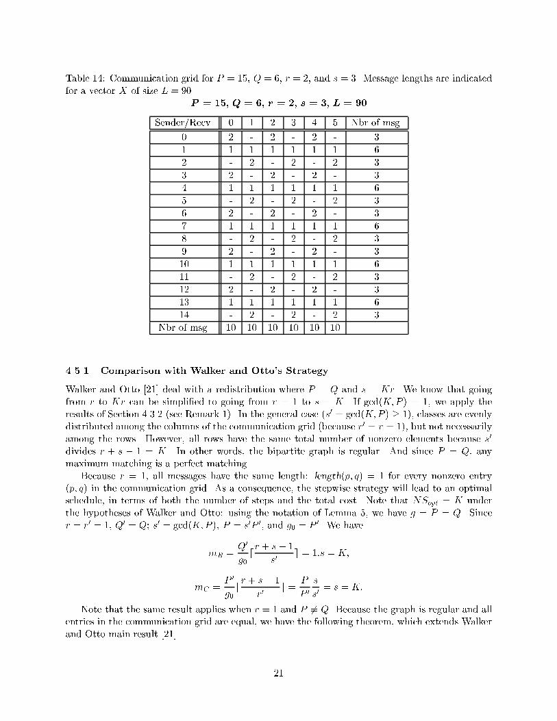
Table 14: Communication grid for P = 15, Q = 6, r = 2, and s = 3. Message lengths are indicated
for a vector X of size L = 90.
P = 15, Q = 6, r = 2, s = 3, L = 90
Sender/Recv. 0 1 2 3 4 5 Nbr of msg.
0 2 - 2 - 2 - 3
1 1 1 1 1 1 1 6
2 - 2 - 2 - 2 3
3 2 - 2 - 2 - 3
4 1 1 1 1 1 1 6
5 - 2 - 2 - 2 3
6 2 - 2 - 2 - 3
7 1 1 1 1 1 1 6
8 - 2 - 2 - 2 3
9 2 - 2 - 2 - 3
10 1 1 1 1 1 1 6
11 - 2 - 2 - 2 3
12 2 - 2 - 2 - 3
13 1 1 1 1 1 1 6
14 - 2 - 2 - 2 3
Nbr of msg. 10 10 10 10 10 10
4.5.1 Comparison with Walker and Otto's Strategy
Walker and Otto [21] deal with a redistribution where P = Q and s = Kr. We know that going
from r to Kr can be simpli�ed to going from r = 1 to s = K. If gcd(K;P ) = 1, we apply the
results of Section 4.3.2 (see Remark 1). In the general case (s0 = gcd(K;P ) � 1), classes are evenly
distributed among the columns of the communication grid (because r0 = r = 1), but not necessarily
among the rows. However, all rows have the same total number of nonzero elements because s0
divides r + s � 1 = K. In other words, the bipartite graph is regular. And since P = Q, any
maximum matching is a perfect matching.
Because r = 1, all messages have the same length: length(p; q) = 1 for every nonzero entry
(p; q) in the communication grid. As a consequence, the stepwise strategy will lead to an optimal
schedule, in terms of both the number of steps and the total cost. Note that NSopt = K under
the hypotheses of Walker and Otto: using the notation of Lemma 5, we have g = P = Q. Since
r = r0 = 1, Q0 = Q; s0 = gcd(K;P ), P = s0P 0, and g0 = P 0. We have
mR =Q0
g0dr + s� 1
s0e = 1:s = K;
mC =P 0
g0dr + s� 1
r0e =
P
P 0
s
s0= s = K:
Note that the same result applies when r = 1 and P 6= Q. Because the graph is regular and all
entries in the communication grid are equal, we have the following theorem, which extends Walker
and Otto main result [21].
21

Table 15: Communication steps (stepwise strategy) for P = 15, Q = 6, r = 2, and s = 3.
Stepwise strategy for P = 15, Q = 6, r = 2, and s = 3
Sender/Recv. 0 1 2 3 4 5
0 a - b - c -
1 h i j e g f
2 - b - c - a
3 b - c - a -
4 j e i h f g
5 - c - a - b
6 c - a - b -
7 i h f g j d
8 - a - b - c
9 f - e - d -
10 g j d f i h
11 - g - d - e
12 d - h - e -
13 e f g j h i
14 - d - i - j
Table 16: Communication costs (stepwise strategy) for P = 15, Q = 6, r = 2, and s = 3.
Stepwise strategy for P = 15, Q = 6, r = 2, and s = 3
Step a b c d e f g h i j Total
Cost 2 2 2 2 2 2 2 2 2 2 20
Proposition 6 Consider a redistribution problem with r = 1 (and arbitrary P , Q and s). The
schedule generated by the stepwise strategy is optimal, in terms of both the number of steps and the
total cost.
The strategy presented in this article makes it possible to directly handle a redistribution from
an arbitrary CYCLIC(r) to an arbitrary CYCLIC(s). In contrast, the strategy advocated by Walker
and Otto requires two redistributions: one from CYCLIC(r) to CYCLIC(lcm(r,s)) and a second
one from CYCLIC(lcm(r,s)) to CYCLIC(s).
5 MPI Experiments
This section presents results for runs on the Intel Paragon for the redistribution algorithm described
in Section 4.
22

Table 17: Communication steps (greedy strategy) for P = 15, Q = 6, r = 2, and s = 3.
Greedy strategy for P = 15, Q = 6, r = 2, and s = 3
Sender/Recv. 0 1 2 3 4 5
0 a - b - c -
1 j k l h g i
2 - b - c - a
3 b - c - a -
4 i g h f e j
5 - c - a - b
6 c - a - b -
7 h e g i j d
8 - a - b - c
9 e - f - d -
10 f i d g h k
11 - f - d - e
12 d - e - f -
13 g h i j k l
14 - d - e - f
Table 18: Communication costs (greedy strategy) for P = 15, Q = 6, r = 2, and s = 3.
Greedy strategy for P = 15, Q = 6, r = 2, and s = 3
Step a b c d e f g h i j k l Total
Cost 2 2 2 2 2 2 1 1 1 1 1 1 18
5.1 Description
Experiments have been executed on the Intel Paragon XP/S 5 computer with a C program calling
routines from the MPI library. MPI is chosen for portability and reusability reasons. Schedules
are composed of steps, and each step generates at most one send and/or one receive per processor.
Hence we used only one-to-one communication primitives from MPI.
Our main objective was a comparison of our new scheduling strategy against the current re-
distribution algorithm of ScaLAPACK [15], namely, the \caterpillar" algorithm that was brie y
summarized in Section 3.2. To run our scheduling algorithm, we proceed as follows:
1. Compute schedule steps using the results of Section 4.
2. Pack all the communication bu�ers.
3. Carry out barrier synchronization.
4. Start the timer.
5. Execute communications using our redistribution algorithm (resp. the caterpillar algorithm).
23

6. Stop the timer.
7. Unpack all bu�ers.
The maximum of the timers is taken over all processors. We emphasize that we do not take the
cost of message generation into account: we compare communication costs only.
Instead of the caterpillar algorithm, we could have used the MPI ALLTOALLV communication
primitive. It turns out that the caterpillar algorithm leads to better performance than the MPI ALLTOALLV
for all our experiments (the di�erence is roughly 20% for short vectors and 5% for long vectors).
We use the same physical processors for the input and the output processor grid. Results are
not very sensitive to having the same grid or disjoint grids for senders and receivers.
5.2 Results
Three experiments are presented below. The �rst two experiments use the schedule presented in
Section 4.3.2, which is optimal in terms of both the number of steps NS and the total cost TC.
The third experiment uses the schedule presented in Section 4.4, which is optimal only in terms of
NS.
Back to Example 1
The �rst experiment corresponds to Example 1, with P = Q = 16, r = 3, and s = 5. The
redistribution schedule requires 7 steps (see Table 3). Since all messages have same length, the
theoretical improvement over the caterpillar algorithm, which as 16 steps, is 7=16 � 0:44. Figure 2
shows that there is a signi�cant di�erence between the two execution times. The theoretical ratio
is obtained for very small vectors (e.g., of size 1200 double-precision reals). This result is not
surprising because start-up times dominate the cost for small vectors. For larger vectors the ratio
varies between 0:56 and 0:64. This is due to contention problems: our scheduler needs only 7 step,
but each step generates 16 communications, whereas each of the 16 steps of the caterpillar algorithm
generates fewer communications (between 6 and 8 per step), thereby generating less contention.
Back to Example 2
The second experiment corresponds to Example 2, with P = Q = 16 processors, r = 7, and s = 11.
Our redistribution schedule requires 16 steps, and its total cost is TC = 77 (see Table 6). The
caterpillar algorithm requires 16 steps, too, but at each step at least one processor sends a message
of length (proportional to) 7, hence a total cost of 112. The theoretical gain 77=112 � 0:69 is to be
expected for very long vectors only (because of start-up times). We do not obtain anything better
than 0:86, because of contentions. Experiments on an IBM SP2 or on a Network of Workstations
would most likely lead to more favorable ratios.
Back to Example 4
The third experiment corresponds to Example 4, with P = 12, Q = 8, r = 4, and s = 3. This
experiment is similar to the �rst one in that our redistribution schedule requires much fewer steps
(4) than does the caterpillar (12). There are two di�erences, however: P 6= Q, and our algorithm
is not guaranteed to be optimal in terms of total cost. Instead of obtaining the theoretical ratio
of 4=12 � 0:33, we obtain results close to 0:6. To explain this, we need to take a closer look at
the caterpillar algorithm. As shown in Table 19, 6 of the 12 steps of the caterpillar algorithm are
indeed empty steps, and the theoretical ratio rather is 4=6 � 0:66.
24

0 50000 100000 150000Global size of redistributed vector (64-bit double precision)
0
5000
10000
15000
Micro
seco
nds
P = Q = 16, r = 3 and s = 5.
caterpillaroptimal scheduling
Figure 2: Comparing redistribution times on the Intel Paragon for P = Q = 16, r = 3 and s = 5.
Table 19: Communication costs for P = 12; Q = 8, r = 4, and s = 3 with the caterpillar schedule.
Caterpillar for P = 12, Q = 8, r = 4, and s = 3
Step a b c d e f g h i j k l Total
Cost 3 0 0 0 3 3 3 0 0 0 3 3 18
6 Conclusion
In this article, we have extendedWalker and Otto's work in order to solve the general redistribution
problem, that is, moving from a CYCLIC(r) distribution on a P -processor grid to a CYCLIC(s)
distribution on a Q-processor grid. For any values of the redistribution parameters P , Q, r, and s,
we have constructed a schedule whose number of steps is optimal. Such a schedule has been shown
optimal in terms of total cost for some particular instances of the redistribution problem (that
include Walker and Otto's work). Future work will be devoted to �nding a schedule that is optimal
in terms of both the number of steps and the total cost for arbitrary values of the redistribution
problem. Since this problem seems very di�cult (it may prove NP-complete), another perspective
is to further explore the use of heuristics like the greedy algorithm that we have introduced, and
to assess their performances.
We have run a few experiments, and these generated optimistic results. One of the next releases
of the ScaLAPACK library may well include the redistribution algorithm presented in this article.
25

0 50000 100000 150000Global size of redistributed vector (64-bit double precision)
2000
4000
6000
8000
10000M
icro
seco
nds
P = Q = 16, r = 7 and s = 11..
caterpillaroptimal scheduling
Figure 3: Time measurement for caterpillar and greedy schedule for di�erent vector sizes, redis-
tributed from P = 16, r = 7 to Q = 16, s = 11.
References
[1] C. Ancourt, F. Coelho, F. Irigoin, and R. Keryell. A linear algebra framework for static
HPF code distribution. Scienti�c programming, to appear. Avalaible as CRI{Ecole des Mines
Technical Report A-278-CRI, and at http://www.cri.ensmp.fr.
[2] Claude Berge. Graphes et hypergraphes. Dunod, 1970.
[3] S. Chatterjee, J. R. Gilbert, F. J. E. Long, R. Schreiber, and S.-H. Teng. Generating local ad-
dresses and communication sets for data-parallel programs. Journal of Parallel and Distributed
Computing, 26(1):72{84, 1995.
[4] J. Choi, J. Demmel, I. Dhillon, J. Dongarra, S. Ostrouchov, A. Petitet, K. Stanley, D. Walker,
and R. C. Whaley. ScaLAPACK: A portable linear algebra library for distributed memory
computers - design issues and performance. Computer Physics Communications, 97:1{15, 1996.
(also LAPACK Working Note #95).
26

0 50000 100000 150000Global size of redistributed vector (64-bit double precision)
0
5000
10000
15000
Micro
seco
nds
P = 12, Q = 8, r = 4 and s = 3.
caterpillaroptimal scheduling
Figure 4: Time measurement for caterpillar and greedy schedule for di�erent vector sizes, redis-
tributed from P = 15, r = 4 to Q = 6, s = 3.
[5] J. J. Dongarra and D. W. Walker. Software libraries for linear algebra computations on high
performance computers. SIAM Review, 37(2):151{180, 1995.
[6] Gene H. Golub and Charles F. Van Loan. Matrix computations. Johns Hopkins, 2 edition,
1989.
[7] R.L. Graham, M. Gr�otschel, and L. Lov�asz. Handbook of combinatorics. Elsevier, 1995.
[8] S. K. S. Gupta, S. D. Kaushik, C.-H. Huang, and P. Sadayappan. Compiling array expressions
for e�cient execution on distributed-memory machines. Journal of Parallel and Distributed
Computing, 32(2):155{172, 1996.
[9] J.E. Hopcroft and R.M. Karp. An n5=2 algorithm for maximum matching in bipartite graphs.
SIAM J. Computing, 2(4):225{231, 1973.
[10] E. T. Kalns and L. M. Ni. Processor mapping techniques towards e�cient data redistribution.
IEEE Trans. Parallel Distributed Systems, 6(12):1234{1247, 1995.
[11] K. Kennedy, N. Nedeljkovic, and A. Sethi. E�cient address generation for
block-cyclic distributions. In 1995 ACM/IEEE Supercomputing Conference.
http://www.supercomp.org/sc95/proceedings, 1995.
[12] K. Kennedy, N. Nedeljkovic, and A. Sethi. A linear-time algorithm for computing the memory
access sequence in data-parallel programs. In Fifth ACM SIGPLAN Symposium on Principles
and Practice of Parallel Programming, pages 102{111. ACM Press, 1995.
27

[13] Charles H. Koelbel, David B. Loveman, Robert S. Schreiber, Guy L. Steele Jr., and Mary E.
Zosel. The High Performance Fortran Handbook. The MIT Press, 1994.
[14] Antoine Petitet. Algorithmic redistribution methods for block cyclic decompositions. PhD
thesis, University of Tennessee at Knoxville, December 1996.
[15] L. Prylli and B. Tourancheau. E�cient block-cyclic data redistribution. In EuroPar'96, volume
1123 of Lectures Notes in Computer Science, pages 155{164. Springer Verlag, 1996.
[16] M. Snir, S. W. Otto, S. Huss-Lederman, D. W. Walker, and J. Dongarra. MPI the complete
reference. The MIT Press, 1996.
[17] J. M. Stichnoth, D. O'Hallaron, and T. R. Gross. Generating communication for array state-
ments: design, implementation, and evaluation. Journal of Parallel and Distributed Computing,
21(1):150{159, 1994.
[18] A. Thirumalai and J. Ramanujam. Fast address sequence generation for data-parallel programs
using integer lattices. In C.-H. Huang, P. Sadayappan, U. Banerjee, D. Gelernter, A. Nicolau,
and D. Padua, editors, Languages and Compilers for Parallel Computing, volume 1033 of
Lectures Notes in Computer Science, pages 191{208. Springer Verlag, 1995.
[19] K. van Reeuwijk, W. Denissen, H. J. Sips, and E. M.R.M. Paalvast. An implementation
framework for HPF distributed arrays on message-passing parallel computer systems. IEEE
Trans. Parallel Distributed Systems, 7(9):897{914, 1996.
[20] A. Wakatani and M. Wolfe. Redistribution of block-cyclic data distributions using MPI. Par-
allel Computing, 21(9):1485{1490, 1995.
[21] David W. Walker and Steve W. Otto. Redistribution of block-cyclic data distributions using
MPI. Concurrency: Practice and Experience, 8(9):707{728, 1996.
[22] Lei Wang, James M. Stichnoth, and Siddhartha Chatterjee. Runtime performance of paral-
lel array assignment: an empirical study. In 1996 ACM/IEEE Supercomputing Conference.
http://www.supercomp.org/sc96/proceedings, 1996.
28