Simultaneous Cyclic Scheduling and Control ofTubular Reactors: Single Production Lines

Antonio Flores-Tlacuahuac∗

Departamento de Ingenierıa y Ciencias Quımicas, Universidad Iberoamericana

Prolongacion Paseo de la Reforma 880, Mexico D.F., 01210, Mexico

Ignacio E. GrossmannDepartment of Chemical Engineering, Carnegie-Mellon University

5000 Forbes Av., Pittsburgh 15213, PA

July 19, 2010

∗Author to whom correspondence should be addressed. E-mail: antonio.flores@uia.mx, phone/fax: +52(55)59504074,http://200.13.98.241/∼antonio

1

Abstract

In this work we propose a simultaneous scheduling and control optimization formulation to address

both optimal steady-state production and dynamic product transitions in continuous multiproduct

tubular reactors. The simultaneous scheduling and control problem for continuous multiproduct

tubular reactors is cast as a Mixed-Integer Dynamic Optimization (MIDO) problem. The dynamic

behavior of the tubular reactor is represented by a set of nonlinear partial differential equations that

are merged with the set of algebraic equations representing the optimal schedule production model. By

using the method of lines, the process dynamic behavior is approximated by a set of nonlinear ordinary

differential equations. Moreover, time discretization of the underlying system allows us to transform

the problem into a Mixed-Integer Nonlinear Programming (MINLP) problem. Three multiproduct

continuous tubular reactors are used as examples for testing the simultaneous scheduling and control

optimization formulation.

2

1 Introduction

Modern society demands large amounts of some commodities such as polymer products. In fact, most of

these products, such as polyethylene, poly-methyl-methacrylate, polystyrene, etc., are manufactured using

continuous production facilities, rather than batch or semi-batch equipment. The reason is that contin-

uous production plants are able to significantly increase productivity in comparison with noncontinuous

processes. In the specific case of the polymer industry continuous stirred tank reactors (CSTR), tubular

reactors (PFR), or a variation/combination of them, have been used as continuous plants for manufactur-

ing polymers. Each one of them presents advantages and disadvantages. For instance, it is widely known

that polymerization reactors carried out in autoclaves are prone to suffer runaway temperature problems

because of the presence of hot spots [1]. Moreover, because some autoclave polymerization reactors are

operated around extreme temperature and pressure processing conditions, acceptable closed-loop control

can be hard to achieve. Operability problems faced by CSTRs are instead usually better handled by using

tubular reactors. In fact, better control temperature in highly exothermic polymerization reaction systems

can be achieved by carrying out such reactions in PFRs facilities. Moreover, a single PFR can feature

the same productivity targets as a battery of CSTRs, potentially leading to a reduction in capital and

operating costs. Mathematical modeling, in conjunction with a strong experimental program is a powerful

way to improve our understanding of complex reaction processes. However, it should be stressed that both

dynamic simulation and optimization of PFRs are harder to perform because of the distributed nature of

tubular reactors. Moreover, the highly nonlinear nature of many industrially relevant reactions in terms of

multiple steady-states and oscillatory behavior, to name just a few nonlinearity patterns, leads to difficult

mathematical models especially for process optimization purposes.

The common practice in scheduling and control problems has been to solve them independently. The

solution of scheduling problems provides information regarding the best production sequence, amounts to

be produced, production times, etc, given a profitability index that is to be optimized. In this context,

process dynamics is neglected leading, for instance, to assume constant transition times among all products

to be manufactured. On the other hand, the solution of control problems renders optimal values of the

selected manipulated variables leading, for instance, to minimum transition times. Normally, during

3

transition operations, minimum off-spec material should be also an operation target. During the solution

of control problems we normally assume that the production sequence has been fixed. This assumption

allows us to solve optimal control problems independently of the underlying scheduling problem. However,

it has been widely recognized [2],[3],[4],[5], that scheduling and control problems are tightly integrated

problems and that improved optimal solutions can be obtained by solving both problems simultaneously

rather than independently, because interactions between problems are explicitly taken into account [6],[7].

A literature review on scheduling and control problems can be found elsewhere [6].

In this work we extend the results reported in [6] to address the simultaneous scheduling and control

problem in a single tubular reactor that manufactures multiple products. As was done in [6], we merge

optimization formulations for dealing with scheduling and optimal control problems. Working along these

lines, the problem is cast as an optimization problem featuring integer and continuous variables, and

because states and manipulated variables are time dependent, the underlying optimization problem is

a mixed-integer dynamic optimization (MIDO) problem. To solve the MIDO problem we have selected

to transform it into a mixed-inter nonlinear program (MINLP). We should stress that because tubular

reactors represent distributed parameter systems, its numerical treatment is normally harder to deal with

than for aggregated systems (the type of dynamic systems addressed in [6]). This is especially true for the

optimization of such a distributed parameter systems. The proposed strategy for solving MIDO problems

featuring distributed parameter systems consists of the spatial and time discretization of the PDAE system

leading to a final set of nonlinear equations. The spatial discretization is approached by using the method

of lines [8], whereas the temporal discretization is addressed using the orthogonal collocation method on

finite elements [9]. Because the resulting MINLP formulation features non-convexities, the solution of

the underlying MINLP was obtained by using the sbb/CONOPT solver embedded in the gams environment.

Recently some open source software for MINLP has become available [10]. Moreover, we propose the use

of a decomposition method for addressing the solution of the scheduling and control problems of the MIDO

case studies addressed in this work. This point is relevant because without an efficient initialization and

decomposition method most of the large scale MIDO problems (as the ones addressed in the present work)

turns out to be difficult or impossible to solve.

4

2 Problem definition

Given are a number of products that are to be manufactured in a single continuous multiproduct PFR.

The corresponding steady-state operating conditions for the production of each product are computed as

part of the solution strategy. The demand rate, the cost of products, raw materials and inventories must

be also specified. Using this information and the SC optimization formulation the problem consists of the

simultaneous determination of the best production wheel (i.e. cyclic time and the sequence in which the

products will be manufactured) as well as the transition times, production rates, length of processing times,

amounts manufactured of each product, such that the profit is maximized subject to a set of scheduling

and dynamic state constraints.

3 Scheduling and Control MIDO Formulation

To tackle the simultaneous scheduling and control (SSC) problem, we assume that all products are pro-

duced in a single tubular reactor. Moreover, all the products will be manufactured using optimal sequences

(i.e. production wheels) to be determined as part of the solution of the SSC problem, where each sequence

is repeated cyclically over an infinite time horizon (see Pinto and Grossmann [11] for the scheduling for-

mulation). For modeling purposes the time is divided into a set of slots as depicted in Figure 1(a). Each

slot is divided in a transition period and in a production period. As part of the solution of the SSC

problem each slot features the production of a single product. Therefore, when a transition operation

is enforced the operating conditions are changed from the old to the new product. Normally, for profit

maximization product transitions should feature minimum transition time. During product transition the

dynamic behavior of the system states and manipulated variables changes as a function of time. This

behavior is conceptually represented in Figure 1(b). Once the system reaches the desired product, the

production period starts and last until the production demands are met. It is worth to mention that when

a production wheel is over then new identical production wheels start again.

Because the SSC optimization formulation used in this work is similar to a previously SSC formulation

aimed to address continuous tank reactors [6], we have summarized the optimization formulation in the

5

Slot 1 Slot 2 Slot Ns

Production Period

Transition period

Cyclic time(a)

Transition Period Production period

x

u

Stat

e, C

ontr

ol v

aria

bles

(b)

Figure 1: (a) At each production period the cyclic time is divided into Ns slots. (b) When a change in theset-point of the system occurs there is a transition period followed by a continuous production period.

appendix section. This material has been included only for completeness. It is worth to mention that

the only difference between the optimization formulation used in [6] and in the present work lies in

the specific type of dynamic system. In [6] the dynamic system is composed by a system of ordinary

differential equations, whereas in the present work the dynamic mathematical models are composed of

a set of partial differential equations. Once the partial differential system is spatially discretized both

optimization formulations become identical.

6

Model Spatial Discretization

In this part, the method of lines was used for the discretization of the spatial partial derivatives [8].

The aim of such a transformation is to replace the spatial partial derivatives by a set of finite difference

equations reducing the original PDE model to a set of ODEs. Hence, the resulting set of ODEs can

be numerically integrated by standard ODEs numerical procedures. In this way both the steady-state

and dynamic behaviour of the original PDE model can be obtained. Although there are some other well

established numerical discretization techniques, such as the finite element [12] and spectral methods [13],

the method of lines is easier to apply to the solution of complex PDE models.

The discretization procedures used in the method of lines are finite difference equations of different degrees

and precision whose aim is to approximate the spatial behavior. The discretization can be done by

using either a fixed or variable domain partition. Because discretization formulas based on fixed domain

partitions are easier to use, in this part we will only use this type of discretization formulas. Mathematical

models of tubular reactors are characterized by featuring diffusive(

∂2C∂x2

)

, convective(

∂C∂x

)

and reaction

terms. Hence, PDE models containing diffusive, convective and reaction terms are termed either diffusion-

convection-reaction or advection-convection-reaction models models.

Taking into account only the diffusive term, the model is classified as a PDE equation of parabolic type,

whereas if only the convective term is considered, then the PDE equation is classified as of a hyperbolic

type [8]. Therefore, the model of the tubular reactor featuring diffusion and convection terms is named

a PDE model of parabolic-hyperbolic type. Moreover, this PDE model classification highlights the fact

that different type of finite elements approximations are required for either parabolic or hyperbolic terms.

Next, the discretization formulas for each type of terms are discussed. For this purpose, the spatial domain

has been divided as depicted in Figure 2. In this figure n stands for the total number of equally spaced

discrete points, xl and xu are the minimum and maximum values of the spatial coordinate x, whereas Δx

is the constant distance between any two adjacent discrete points.

In order to compute a numerical solution to a second degree PDE model, two independent boundary

conditions at certain locations of the reactor must be specified. In this work, Dirichlet (at x = 0) and

7

Neumann (at x = L, where L is the reactor length) boundary conditions are enforced at the inlet and outlet

parts of the reactor, respectively. As shown below, the discretization formulas are different depending upon

the type of boundary conditions, the spatial location of the discretization points, and whether the spatial

derivatives define a parabolic or hyperbolic PDE term.

����

����

����

����

����

����

����

������������������ ����������������������������������

��������������

1 2 3 4 n−1 nn−2

xuxl∆x

Figure 2: The spatial domain is divided into n equally sized discretization intervals denoted by Δx, xl andxu are the lower and upper values of the spatial coordinate.

∙ Diffusive term

1. First point (Dirichlet boundary conditions)

∂2u

∂x2

∣

∣

∣

∣

1

= �(45u1 − 154u2 + 214u3 − 156u4 + 61u5 − 10u6) (1)

2. Interior grid points

∂2u

∂x2

∣

∣

∣

∣

2

= �(10u1 − 15u2 − 4u3 + 14u4 − 6u5 + u6) (2)

∂2u

∂x2

∣

∣

∣

∣

i

= �(−ui−2 + 16ui−1 − 30ui + 16ui+1 − ui+2), i = 3, ..., n− 2 (3)

∂2u

∂x2

∣

∣

∣

∣

n−1

= �(10un − 15un−1 − 4un−2 + 14un−3 − 6un−4 + un−5) (4)

3. Last point (Neumann boundary conditions)

∂2u

∂x2

∣

∣

∣

∣

n

= �(−415

6un + 96un−1 − 36un−2 +

32

3un−3 −

3

2un−4 + 50

∂u

∂x

∣

∣

∣

∣

n

Δx) (5)

8

where,

Δx =xu − xl

n− 1(6)

� =1

12Δx2(7)

∙ Convective term

1. First point

∂u

∂x

∣

∣

∣

∣

1

= (−25u1 + 48u2 − 36u3 + 16u4 − 3u5) (8)

2. Interior grid points

∂u

∂x

∣

∣

∣

∣

2

= (−3u1 − 10u2 + 18u3 − 6u4 + u5) (9)

∂u

∂x

∣

∣

∣

∣

3

= (u1 − 8u2 + 8u4 − u5) (10)

∂u

∂x

∣

∣

∣

∣

i

= (−ui−3 + 6ui−2 − 18ui−1 + 10ui + 3ui+1), i = 4, ..., n− 1 (11)

3. Last point

∂u

∂x

∣

∣

∣

∣

n

= (3un−4 − 16un−3 + 36un−2 − 48un−1 + 25un) (12)

where,

=1

12Δx(13)

4 Case studies

In this section several simultaneous scheduling and control problems taking place in tubular reactors are

addressed. The examples were selected to feature different degrees of steady-state and dynamic nonlinear

behavior, such that the complexity of solving scheduling and control problems is highlighted. We also did

so hoping to justify the use of advanced decomposition optimization techniques such as Lagrangian decom-

position [14] to address the scheduling and control of more complex reaction system such as polymerization

9

reaction systems.

It is a well known fact that most NLP solvers require good initialization strategies to succeed in finding

an optimal solution. This is especially true when the size and model complexity are factors that deserve

careful consideration. In fact, if good initial guesses are not provided, finding even a feasible solution can

be hard to achieve. In our experience, the scheduling and control optimization of distributed parameter

systems can be efficiently tackled by decomposing the original complex problem into a series of simpler

subproblems. The idea is to use the simpler subproblems to initialize more complex versions of the problem

to be solved. In this work, we use the natural decomposition present in scheduling and control problems

to solve simultaneous scheduling and control problems in distributed parameter systems. The approach is

as follows:

1. Solve the scheduling problem by fixing transition times.

2. Compute steady-state processing conditions for the set of products to be manufactured.

3. Solve the dynamic optimization problem by fixing the best production sequence found in step (1)

above.

4. Solve the simultaneous scheduling and control problem by relaxing the computation of the best

production sequence and optimal product transitions.

As indicated, the idea behind the initialization procedure is to use results from a previous step to initialize

the next one. All the simultaneous scheduling and control problems were solved using the above solution

strategy. For the numerical solution of the MINLP problem arising from the discretization of the original

MIDO problem the sbb/CONOPT MINLP solver in gams [15] was used. After some trials, we came to the

conclusion that 11 equal sized points were enough for spatial discretization, whereas 20 finite elements and

3 internal collocation points sufficed for time discretization. Moreover, all the problems were solved using

2 Ghz, 4 Gb computer.

10

Isothermal tubular reactor

The reaction 2A → B takes place in a continuous tubular reactor. For modeling this reaction system we

assume isothermal conditions, plug flow conditions and mass transfer along the longitudinal direction. Both

diffusive and convective mass transfer contributions are also modeled. Under these operating conditions

the one-dimensional dynamic mathematical model of the tubular reactor reads as follows:

∂C

∂t= D

∂2C

∂x2− v

∂C

∂x−KC2 (14)

subject to the following initial,

C(x, 0) = Cf (15)

and boundary conditions,

@ x = 0 C = Cf +D

v

∂C

∂x(16)

@ x = L∂C

∂x= 0 (17)

where C stands for the concentration of the A component, x is the longitudinal coordinate, t is the time,

D is the mass diffusivity and v is the linear velocity, K is the reaction constant, Cf is the feed stream

composition of reactant A and L is the reactor length. The above model can be cast in dimensionless form

by using the following dimensionless variables:

C′

=C

Cf

, x′

=x

L, � =

tv

L

Hence, in terms of the dimensionless variables, the scaled model reads as follows,

∂C′

∂�=

1

PeM

∂2C′

∂x′2

−∂C

′

∂x′−

�

PeMC

′2 (18)

11

Product Conversion Demand Process Inventory Transition Cost [$]fraction rate [Kg/h] cost [$/kg] cost [$/kg] A B C D E

A 0.5024 100 620 1.5 0 350 700 600 400B 0.6036 90 730 1 400 0 550 450 500C 0.6959 120 750 2 800 600 0 550 800D 0.8019 80 770 3 500 400 600 0 700E 0.9 70 790 2.5 600 370 550 700 0

Table 1: Process data for the isothermal tubular reactor case study. A,B,C,D and E stand for the fiveproducts to be manufactured.

subject to the following initial,

C′

(x′

, 0) = 1 (19)

and dimensionless boundary conditions,

@ x = 0∂C

′

∂x′= PeM(C

′

− 1) (20)

@ x = 1∂C

′

∂x′= 0 (21)

where PeM = LvD

is the mass transfer Peclet number and � =L2KCf

D. Using L = 20 m, D = 10 m2/s,

Cf=100 kmol/m3, r=0.5 m and K =1x10−3 m3/kmol-h, lead to the production of five products A,B,C,D

and E which are defined in Table 1. In addition, Table 1 contains information regarding the cost of the

products, demand rate, inventory cost, and production rate of each one of the hypothetical products. The

manipulated variable for optimal product transitions is the volumetric flow rate.

The optimal production sequence resulting from the simultaneous scheduling and control problem turns

out to be: D → B → A → E → C, the duration time of the cyclic production sequence is 252.031 h,

featuring a profit of $1.013x106. The optimal solution was obtained in 55 min CPU time. The number of

equations, continuous and discrete variables is 14846, 15217 and 50, respectively. In Table 2, a summary

of the results of the optimal solution is shown, whereas the optimal dynamic transition profiles among the

manufactured products are depicted in Figure 3. We should note that this solution is not guaranteed to

be globally optimal due to the nonconvexities in the MINLP model.

12

Volumetric Conc. � Amount Production Process T start T endSlot Prod. Flow [m3/s] [kmol/m3] [h] Produced [Kg] rate [kg/h] time [h] [h] [h]1 D 0.1 19.8 2 20162.489 762.872 26.43 0 31.432 B 0.62 39.6 2.5 22682.801 3555.098 6.38 31.43 42.813 A 1.169 49.8 0.5 4.2360x105 5580.029 75.91 42.81 123.724 E 0.02 10 1.5 17642.178 170.978 103.18 123.72 231.95 C 0.302 30.4 0.5 30243.734 1999.680 15.12 231.9 252.03

Table 2: Simultaneous Scheduling and Control results for the isothermal tubular reactor case study. Thebest production sequence is: D → B → A → E → C featuring 252.031 h as total cyclic time andobjective function value of $1.013x106. The optimal solution was computed in 55 min CPU time. � standsfor discretized transition times.

0 0.5 1 1.5 2 2.5 3 3.5 4 4.5 50

10

20

30

40

50

60

Time [h]

Conc

entra

tion

[kmol/

m3 ]

DBAEC

(a)

0 0.5 1 1.5 2 2.5 3 3.5 4 4.5 50

0.2

0.4

0.6

0.8

1

1.2

1.4

Time [h]

Volum

etric

flowr

ate

[m3 /s]

DBAEC

(b)

Figure 3: Optimal dynamic transition profiles for the isothermal tubular reactor. The best productionsequence is: D → B → A → E → C.

13

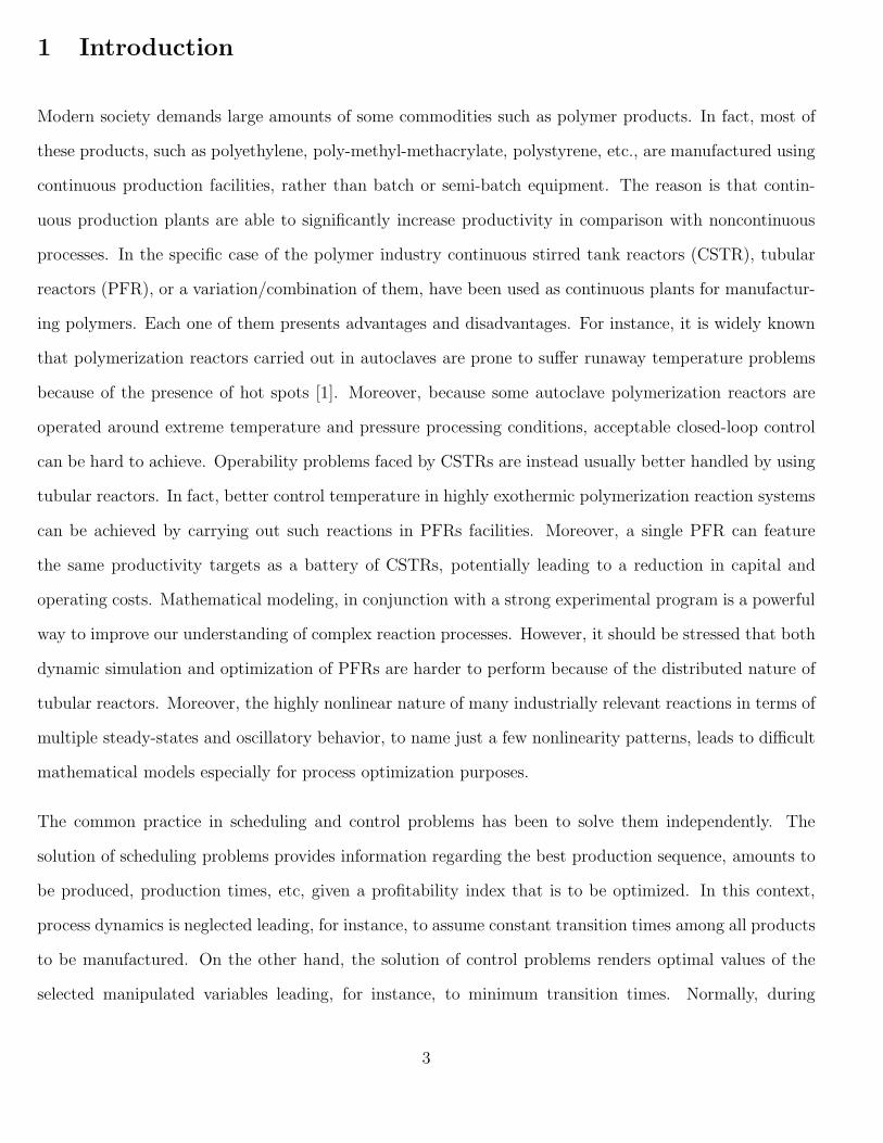
It should be pointed out that there are other optimal production sequences that are equivalent to the

one found previously. This means that these optimal sequences feature the same objective function value,

cyclic time, amount produced, production rate, processing time, etc. For instance, the sequences B →

A → E → C → D and A → E → C → D → B are equivalent to the aforementioned optimal production

sequence. Due to the cyclic production wheel assumption, it is completely irrelevant whether product D is

actually manufactured at the first, second, third, fourth or fifth slot. All the equivalent optimal production

sequences feature the same production order. However, we have found that equivalent optimal sequences

tend to demand different CPU times for finding an optimal solution.

Regarding the optimal dynamic transition profiles, as depicted in Figure 3, the system response is, in

general, smooth. This is especially true when the product transition involves reducing product conversion

as done in slots where products D, B and E are manufactured. When the product transition involves

increasing product conversion, as in the slots where products C and A are manufactured, an inverse

response is observed. In fact, this effect is more notorious for product A. However, at the end of the

transition period, all the products attain the final steady-state operating conditions. On the other hand,

the manipulated variable assumes ramp-like changes with large slopes. Looking at Figure 3, the reasons of

the aforementioned apparent system inverse response behavior become clear. In the case of products D,

B and E, the manipulated variable response takes a ramp-like shape without changes in the slope sign.

However, in those cases where an inverse response is observed, products C and A, there are some changes

in the sign of the slope during the product transition. It may be argued whether by using simple step

changes in the manipulated variable, one could get similar results to the ones shown in Figure 3. This may

be apparent after the fact, but it is hard to guess before carrying out all the optimal dynamic transition

calculations. Anyway, our results feature optimality characteristics, a point that cannot be raised in favor

of simple step changes.

14

Nonisothermal plug-flow tubular reactor

Let us consider the nonisothermal operation of a one-dimensional tubular reactor where the set of reactions

is given by:

Ak10→ B

k20→ C

By assuming plug-flow, negligible temperature and concentration radial variations and no diffusion along

the axial spatial coordinate, the distributed mathematical model of the systems reads as follows [16]:

∂CA

∂t= −v

∂CA

∂x− k10e

−E1/RTrCA (22)

∂CB

∂t= −v

∂CB

∂x+ k10e

−E1/RTrCA − k20e−E2/RTrCB (23)

∂Tr

∂t= −v

∂Tr

∂x+

(−ΔHRA)

�mCpmk10e

−E1/RTrCA

−(−ΔHRB

)

�mCpm

k20e−E2/RTrCB +

UwA

�mCpmVr

(Tj − Tr) (24)

where CA is the concentration of component A, CB is the concentration of component B, Tr is the reactor

temperature, t is stands for time, x denotes the length of the reactor and v is the linear velocity. The

meaning of the rest of the variables and their corresponding numerical values are shown in Table 3. The

aforementioned model is subject to the following initial

CA∣x,t=0 = CsA (25)

CB∣x,t=0 = CsB (26)

Tr∣x,t=0 = T sr (27)

and boundary conditions:

CA∣x=0,t = CfA (28)

CB∣x=0,t = CfB (29)

Tr∣x=0,t = T fr (30)

15

where the superscripts s, f stand for steady-state processing conditions and feed stream conditions, re-

spectively. By defining the following dimensionless variables:

CA =CA

CfA

(31)

CB =CB

CfA

(32)

Tr =Tr

Tfr

(33)

Tj =Tj

Tfr

(34)

x =x

L(35)

� =tv

L(36)

the dimensionless PDE model reads as follows:

∂CA

∂�= −

∂CA

∂x−

k10L

ve−E1/RT f

r TrCA (37)

∂CB

∂�= −

∂CB

∂x+

k10L

ve−E1/RT f

r TrCA −k20L

ve−E2/RT f

r TrCB (38)

∂Tr

∂�= −

∂Tr

∂x+

(−ΔHRAk10C

fA)

�mCpmTfr v

e−E1/RT fr TrCA

−(−ΔHRB

k20CfAL)

�mCpmTfr v

e−E2/RT fr TrCB +

UwAL

�mCpmVrv(Tj − Tr) (39)

and the corresponding initial

CA∣x,�=0 =Cs

A

CfA

(40)

CB∣x,�=0 =Cs

B

CfA

(41)

Tr∣x,�=0 =T sr

Tfr

(42)

16

Variable Description Value UnitsL reactor length 1 mE1 activation energy first reaction 20000 kcal/gmolE2 activation energy second reaction 50000 kcal/kgmolk10 pre-exponential factor first reaction 5x1012 1/mink20 pre-exponential factor second reaction 5x1012 1/minΔHRA

heat of reaction of first reaction -0.548 kcal/kgmolΔHRB

heat of reaction of second reaction -0.986 kcal/kgmol�m density of reacting mixture 0.09 kg/LA heat transfer area 1 m2

R ideal gas constant 1.987 kcal/kgmol-KUw heat transfer coefficient 2 kcal/m2-K-minCpm reacting mixture heat capacity 0.231 kcal/kg-KMwA

molecular weight compound A 200 kg/kmolMwB

molecular weight compound B 190 kg/kmol

CfA reactant A feed stream composition 4x10−3 Kmol/L

CfB product B feed steam composition 0 Kmol/L

T fr reactor feed stream temperature 320 K

Tj cooling fluid stream temperature 352 KVr reactor volume 10 L

Table 3: Design data for the nonisothermal plug-flow tubular reactor case study.

and boundary dimensionless conditions:

CA∣x=0,� = 1 (43)

CB∣x=0,� = 1 (44)

Tr∣x=0,� = 1 (45)

Information regarding the desired products, conversion fraction, demand, cost of the products and inven-

tory cost are shown in Table 4. The variable used as manipulated variable for optimal product transitions

is the linear velocity v.

The optimal production sequence resulting from the simultaneous scheduling and control problem turns

out to be: A → B → C → E → D, the duration time of the cyclic production sequence is 137.598 h,

featuring a profit of $22816.78. The optimal solution was obtained in 1.15 h CPU time. The number of

equations, continuous and discrete variables is 33566, 37357 and 50, respectively. In Table 5, a summary

17

Product Conversion Demand Process Inventory Transition Cost [$]Fraction rate [Kg/m] cost [$/kg] cost [$/kg] A B C D E

A 0.5 6 150 1.5 0 5 6 7 8B 0.6 8 200 1 10 0 5 8 6C 0.7 7 240 2 7 10 0 8 7D 0.8 6 280 3 6 10 10 0 12E 0.9 5 320 2.5 8 9 10 10 0

Table 4: Process data for the non-isothermal plug-flow tubular reactor case study. A,B,C,D and E standfor the five products to be manufactured.

of the results of the optimal solution are shown, whereas the optimal dynamic transition profiles among

the manufactured products are depicted in Figure 4.

v � Amount Production Process T start T end

Slot Prod. CA CB Tr [m/min] [h] Produced [Kg] rate [kg/m] time [h] [h] [h]1 A 0.5 0.5 1.151 4.269 2 825.59 129.115 6.4 0 11.392 B 0.4 0.6 1.155 3.765 1.8 1100.787 136.674 8.05 11.39 24.443 C 0.3 0.7 1.159 3.309 1.6 963.188 140.129 6.87 24.44 36.324 E 0.1 0.9 1.166 2.858 2.1 10896.744 127.734 85.3 36.32 126.635 D 0.2 0.8 1.163 2.346 2.2 825.59 138.335 5.97 126.63 137.6

Table 5: Simultaneous Scheduling and Control results for the non-isothermal plug flow tubular reactorcase study. The best production sequence is: A → B → C → E → D featuring 137.598 h as total cyclictime and objective function value of $22816.78. The optimal solution was computed in 1.55 h CPU time.� stands for transition times.

Regarding the optimal dynamic transition profiles shown in Figure 4, we note that all the system responses

feature smooth behavior. In this case no system inverse response was observed. This is so because the

manipulated variable takes a ramp-like shape without changing the sign of their slopes. Once again, one

could be tempted to argue that no dynamic optimization calculations would be needed, if one were to just

use simple step changes in the manipulated variables values. This, however, overlooks several important

points. First, it is hard to guess the optimal shape of the manipulated variables response without actually

calculating the optimal solution. Second, our calculations ensure (local) optimality conditions, whereas

system response obtained by applying simple step-changes does not. Moreover, even when one could guess

the shape of the manipulated variables behavior, it is hard to have good guesses of the optimal production

sequence. Because of these reasons, instead of using a trial and error procedure, we claim that much better

18

results are obtained by solving the scheduling and control problem by a simultaneous approach and within

a formal optimization framework. Finally, it is worth to mention that the present case study demanded

almost twice the CPU time of the first case study. The CPU time increased because of the larger number

of continuous variables, since the present distributed model feature more system states. To keep the CPU

time relatively low, we decided not to increase the number of integers variables. In the next case study, we

will approach a similar distributed parameters system example, but featuring a larger number of integer

variables, just to analyze the effect that increasing the number of binary decision variables has on the CPU

time.

0 0.5 1 1.5 2 2.5 30.05

0.1

0.15

0.2

0.25

0.3

0.35

0.4

0.45

0.5

0.55

Time [h]

Dim

ensio

nless

Con

cent

ratio

n

ABCED

(a)

0 0.5 1 1.5 2 2.5 32

2.5

3

3.5

4

4.5

Time [h]

Flow

veloc

ity [m

/min]

ABCED

(b)

Figure 4: Optimal dynamic transition profiles for the non-isothermal plug-flow tubular reactor. Theoptimal production sequence is: A → B → C → E → D.

19

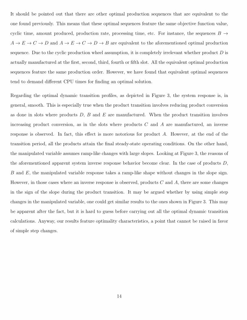
Nonisothermal catalytic fixed-bed tubular reactor

In this example, we use the model of a nonisothermal catalytic fixed-bed tubular reactor. This model

happens to display strong nonlinear behavior, and demands large CPU time for the computation of the

simultaneous scheduling and control optimal solution. The distributed parameter model reads as follows:

∂CA

∂t= −

v

�

∂CA

∂x+

�(1− �)

�

[

−k1e−E1/RTCA − k3e

−E3/RTCA

]

(46)

∂CB

∂t= −

v

�

∂CB

∂x+

�(1− �)

�

[

k1e−E1/RTCA − k2e

−E2/RTCB

]

(47)

∂T

∂t= −

v

Le

∂T

∂x+

�(1− �)

Le�fCpf

[

−ΔHr1k1e−E1/RTCA −ΔHr2k2e

−E2/RTCB

−ΔHr3k3e−E3/RTCA

]

+2UL

Le r′

�fCpf

(Tw − T ) (48)

where CA is the concentration of component A, CB is the concentration of component B, T is the reactor

temperature, t is stands for time, x denotes the length of the reactor, v is the linear velocity and Le =

(1−�)�sCsp+��fCf

p

�fCpcis the Lewis number. The meaning of the rest of the variables, and their corresponding

numerical values are shown in Table 6. The aforementioned model is subject to the following initial

CA∣x,t=0 = CsA (49)

CB∣x,t=0 = CsB (50)

T ∣x,t=0 = T s (51)

20

and boundary conditions:

CA∣x=0,t = CfA +

Dm

v

∂CA

∂x(52)

CB∣x=0,t = CfB +

Dm

v

∂CB

∂x(53)

T ∣x=0,t = T f +Dt

v

∂T

∂x(54)

∂CA

∂x∣x=L,t = 0 (55)

∂CB

∂x∣x=L,t = 0 (56)

∂T

∂x∣x=L,t = 0 (57)

where the superscript s stands for steady-state processing conditions. By defining the following dimen-

sionless variables:

CA =CA

CfA

(58)

CB =CB

CfB

(59)

T =T

T f(60)

Tw =Tw

T f(61)

x =x

L(62)

� =tv

L(63)

the dimensionless PDE model reads as follows:

∂CA

∂�= −

1

�

∂CA

∂x+

L�(1− �)

v�

[

−k1e−E1/RT f T CA − k3e

−E3/RT f T CA

]

(64)

∂CB

∂�= −

1

�

∂CB

∂x+

L�(1− �)

v�

[

k1e−E1/RT f T CA − k2e

−E2/RT f T CB

]

(65)

∂T

∂�= −

1

Le

∂T

∂x+

�(1− �)CfAL

Le�fCpfvT f

[

−ΔHr1k1e−E1/RT f T CA −ΔHr2k2e

−E2/RT f T CB

−ΔHr3k3e−E3/RT f T CA

]

+2UL2

Le r′

�fCpfv(Tw − T ) (66)

21

and the initial:

CA∣x,�=0 =Cs

A

CfA

(67)

CB∣x,�=0 =Cs

B

CfB

(68)

T ∣x,�=0 =T s

T f(69)

and boundary dimensionless conditions:

CA∣x=0,� = 1 +Dm

vL

∂CA

∂x(70)

CB∣x=0,� = 1 +Dm

vL

∂CB

∂x(71)

T ∣x=0,� = 1 +Dt

vL

∂T

∂x(72)

∂CA

∂x∣x=1,� = 0 (73)

∂CB

∂x∣x=1,� = 0 (74)

∂T

∂x∣x=1,� = 0 (75)

Information regarding the desired products, conversion fraction, demand, cost of the products and inven-

tory cost is shown in Table 7. The variable used as manipulated variable for optimal product transitions

is the volumetric flow rate.

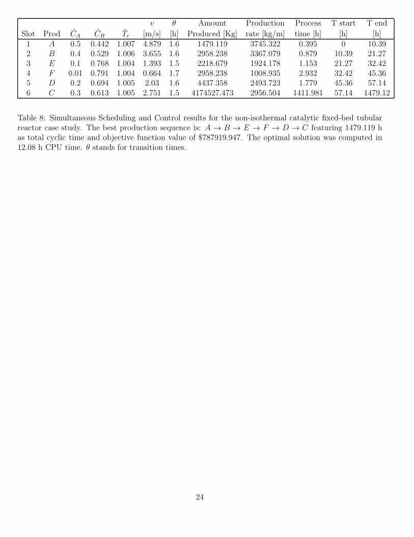
The optimal production sequence resulting from the simultaneous scheduling and control problem turns

out to be: A → B → E → F → D → C, the duration time of the cyclic production sequence is 1479.119

h, featuring a profit of $787919.947. The optimal solution was obtained in 12.08 h CPU. The number

of equations, continuous and discrete decision variables is 40357, 40952 and 72, respectively. In Table

8, a summary of the results about the local optimal solution are shown, whereas the optimal dynamic

transition profiles among the manufactured products are depicted in Figure 5.

22

Variable Description Value UnitsL reactor length 4 m� pellet porosity 0.35k1 reaction rate 2.418x109 1/sk2 reaction rate 2.706x109 1/sk3 reaction rate 1.013x109 1/sE1 exponential factor 1.129x105 J/molE2 exponential factor 1.313x105 J/molE3 exponential factor 1.196x105 J/molΔHr1 heat of reaction -1.285x106 J/KmolΔHr2 heat of reaction -3.276x106 J/KmolΔHr3 heat of reaction -4.561x106 J/Kmol�f feed stream density 0.582 kg/m3

�s catalysts density 2000 kg/m3

Cpf feed stream heat capacity 1045 J/Kg-KCpc coolant fluid heat capacity 483.559 J/Kg-KCps catalysts heat capacity 836 J/Kg-Kr′

reactor radius 0.0125 mU heat transfer coefficient 96.02 J/kg-K-s� catalyst activity 1R ideal gas constant 8.31447 J/mol-KT f feed stream temperature 628 K

CfA reactant A feed stream concentration 0.181 kmol/m3

CfB component B feed stream concentration 0 kmol/m3

Tw heating fluid temperature 630 KDm mass diffusivity 1x10−7 m2/sDt thermal diffusivity 1x10−7 m2/sMwA compound A molecular weight 230 Kg/KgmolMwB compound B molecular weight 200 Kg/Kgmol

Table 6: Design data for the non-isothermal catalytic fixed-bed tubular reactor case study.

Product Conversion Demand Process Inventory Transition Cost [$]Fraction rate [Kg/s] cost [$/kg] cost [$/kg] A B C D E F

A 0.5 1 270 1.5 0 5 6 7 8 9B 0.6 2 280 1 10 0 5 8 6 10C 0.7 1.2 350 2 7 10 0 8 7 11D 0.8 3 380 3 6 10 10 0 12 8E 0.9 1.5 430 2.5 8 9 10 10 0 10F 0.99 2 380 1.2 11 8 7 9 11 0

Table 7: Process data for the non-isothermal catalytic fixed-bed tubular reactor case study. A,B,C,D,E

and F stand for the five products to be manufactured.

23

v � Amount Production Process T start T end

Slot Prod CA CB Tr [m/s] [h] Produced [Kg] rate [kg/m] time [h] [h] [h]1 A 0.5 0.442 1.007 4.879 1.6 1479.119 3745.322 0.395 0 10.392 B 0.4 0.529 1.006 3.655 1.6 2958.238 3367.079 0.879 10.39 21.273 E 0.1 0.768 1.004 1.393 1.5 2218.679 1924.178 1.153 21.27 32.424 F 0.01 0.791 1.004 0.664 1.7 2958.238 1008.935 2.932 32.42 45.365 D 0.2 0.694 1.005 2.03 1.6 4437.358 2493.723 1.779 45.36 57.146 C 0.3 0.613 1.005 2.751 1.5 4174527.473 2956.504 1411.981 57.14 1479.12

Table 8: Simultaneous Scheduling and Control results for the non-isothermal catalytic fixed-bed tubularreactor case study. The best production sequence is: A → B → E → F → D → C featuring 1479.119 has total cyclic time and objective function value of $787919.947. The optimal solution was computed in12.08 h CPU time. � stands for transition times.

24

0 0.5 1 1.5 2 2.5 3 3.5 4 4.5 50

0.1

0.2

0.3

0.4

0.5

0.6

0.7

Time [h]

Dim

ensio

nless

Con

cent

ratio

n

ABEFDC

(a)

0 0.5 1 1.5 2 2.5 3 3.5 4 4.5 50.5

1

1.5

2

2.5

3

3.5

4

4.5

5

Time [h]

Flow

veloc

ity [m

/s]

ABEFDC

(b)

Figure 5: Optimal dynamic transition profiles for the nonisothermal catalytic fixed-bed tubular reactor.The optimal production sequence is: A → B → E → F → D → C.

Similarly to the past case studies, the optimal dynamic transition responses display a smooth behavior,

as shown in Figure 5. Once again, the manipulated variable takes a ramp-like shape, and no inverse

system response behavior is observed. This example clearly shows the impact, in terms of CPU time, of

increasing both the number of integer variables and the perceived nonlinearity of the distributed parameter

model. As a matter fact, in this problem the number of binary variables were 72, 22 more integer variables

when compared to the second case study. Moreover, the number of continuous variables and constraints

between the second and third case studies are similar. However, the computation of the optimal solution

25

of the third case study, required around 6 times the CPU to find an optimal solution with the branch

and bound method in SBB for the second case study. When realizing that the main difference between

these problems lies in the number of binary variables, and that this translates into a larger computational

cost, then it is worth to consider alternative MINLP methods (e.g. Generalized Benders Decomposition,

Outer-Approximation) or solution approaches such as advanced decomposition techniques [14].

5 Conclusions

In this paper we have formulated an extension of our previous work [6], on the simultaneous scheduling

and control optimization problem in continuous stirred tank reactors, to incorporate distributed parameter

systems. Specifically, we have dealt with nonisothermal one-dimensional plug flow reactors, featuring

large dimensionality and highly nonlinear behavior. The proposed simultaneous scheduling and control

optimization formulation was able to successfully solve all the addressed problems, demanding different

computational requirements. After some trials, we found that because the addressed problems feature

simple geometry characteristics, a finite difference scheme [8] was sufficient to discretize the longitudinal

component. This will not be necessarily the case for more complex system geometries, and they probably

will demand more sophisticated discretization strategies such as finite elements [12] and spectral [13]

methods. After spatial discretization, temporal discretization was efficiently handled by using orthogonal

collocation on finite elements [9]. Because of the highly nonlinear system behavior, we used the sbb/CONOPT

branch and bound procedure [15] to address the solution of the underlying MINLPs.

There are several possible research extensions of the present problem. First, product transitions are

more common, but not only, in the polymer industry [3], [17], [18], [19]. Hence, because of complex

kinetics, mass and energy interactions and their distributed nature, the scheduling and control problem

in polymerization tubular reactors presents a formidable computational challenge. In this context, the

computational demands of the problems addressed in this work, suggest that the efficient solution of

the MINLPs problems arising from polymerization tubular reactors will demand special decomposition

optimization techniques as the ones we have used for other types of polymerization reactors [20]. Another

26

extension of the present work deals with the computation of global optimal solutions. We have made some

attempts to compute global optimal solutions of the MINLPs problems addressed in the this work, but

without success, even for the first case study that happens to be the simpler problem. The global optimal

solution of large scale MINLPs seems to be out of reach for most of the distributed parameter systems,

and it is a topic that deservers further research consideration.

27

References

[1] N.K. Read S.X. Zhang and W.H. Ray. Runaway Phenomena in Low-Density Polyethylene Autoclave

Reactors. AIChE J., 42(10):2911–2925, 1996.

[2] T. Bhatia and L.T. Biegler. Dynamic Optimization in the Design and Scheduling of Multiproduct

Batch Plants. Ind. Eng. Chem. Res., 35:2234–2246, 1996.

[3] A.C. Allcock R. Mahadevan, F.J. Doyle III. Scheduling of Polymer Grade Transitions. AIChE J.,

48(8):1754–1764, 2002.

[4] B. V. Mishra, E. Mayer, J. Raisch, and A. Kienle. Short-Term Scheduling of Batch Processes. A

Comparative Study of Differentes Approaches. Ind. Eng. Chem. Res., 44:4022–4034, 2005.

[5] R. H. Nystrom, R. Franke, I. Harjunkoski, and A. Kroll. Production Campaing Planning Including

Grade Transition Sequencing and Dynamic Optimization. Comput. Chem. Eng., 29(10):2163–2179,

2005.

[6] A. Flores-Tlacuahuac and I.E. Grossmann. Simultaneous Cyclic Scheduling and Control of a Multi-

product CSTR. Ind. Eng. Chem. Res., 45(20):6175–6189, 2006.

[7] S. Terrazas-Moreno, A. Flores-Tlacuauhuac, and I.E. Grossmann. Simultaneous scheduling and con-

trol in polymerization reactors. AIChE J., 53(9), 2007.

[8] W. E. Schiesser. The Numerical Method of Lines. Integration of Partial Differential Equations. Aca-

demic Press, Inc., 1991.

[9] L.T. Biegler. An overview of simultaneous strategies for dynamic optimization. Chemical Engineering

and Processing, 46(11):1043–1053, 2007.

[10] Pierre Bonami, Lorenz Biegler, Andrew Conn, Gerard Cornuejols, Ignacio Grossmann, Carl

Laird, Jon Lee, Andrea Lodi, Francois Margot, Sawaya Nicolas, and Andreas Waechter. An

algorithmic framework for convex mixed integer nonlinear programs. Discrete Optimization,

doi:10.1016/j.disopt.2006.10.011, 2007.

28

[11] J.M. Pinto and I. E. Grossmann. Optimal Cyclic Scheduling of Multistage Continuous Multiproduct

Plants. Comput. Chem. Eng., 18(9):797–816, 1994.

[12] Prodromos Daoutidis Nikolaos V. Mantzaris and Friedrich Srienc. Numerical solution of multi-variable

cell population balance models: III. Finite element methods. Comput. Chem. Eng., 25:1463–1481,

2001.

[13] Prodromos Daoutidis Nikolaos V. Mantzaris and Friedrich Srienc. Numerical solution of multi-variable

cell population balance models: II. Spectral methods. Comput. Chem. Eng., 25:1441–1462, 2001.

[14] M. Guinard and S.Kim. Lagrangean Decomposition: A model yielding Stronger Lagrangean Bounds.

Mathematical Programming, 39:215–228, 1987.

[15] A. Brooke, D. Kendrick, Meeraus, and R. A. Raman. GAMS: A User’s Guide. GAMS Development

Corporation, 1998, http://www.gams.com.

[16] W. Wu and S.Y. Ding. Model Predictive Control of Nonlinear Distributed Parameter Systems Using

Spatial Neural-Networks Architectures. Ind. Eng. Chem. Res., 47:7264–7273, 2008.

[17] J.R. Richards J.P. Congalidis and W.H. Ray. Scheduling of Polymer Grade Transitions. AIChE J.,

48(8):1754–1764, 2002.

[18] C. Chatzidoukas, C. Kiparissidis, J.D. Perkins, and Pistikopoulos E.N. Optimal Grade Transition

Campaign Scheduling in a Gas Phase Polyolefin FBR Using Mixed Integer Dynamic Optimization.

Process System Engineering, pages 744–747. Elsevier, 2003.

[19] A. Kroll W. Marquardt A. Prata, J.Oldenburg. Integrated Scheduling and Dynamic Optimization of

Grade Transitions for a Continuous Polymerization Reactor. Comput. Chem. Eng., 32:463–476, 2008.

[20] Sebastian Terrazas-Moreno, Antonio Flores-Tlacuahuac, and Ignacio E. Grossmann. A Lagrangean

Heuristic Approach for the Simultaneous Cyclic Scheduling and Optimal Control of Multi-Grade

Polymerization Reactors. AIChE J., 54(1):163–182, 2008.

29

A Simultaneous Scheduling and Control Optimization Formu-

lation

This section contains the simultaneous scheduling and control optimization formulation previously pub-

lished in [6] and it has been included in the present work only for completeness reasons. A complete

description of the meaning of the objective function and constraints can be found elsewhere [6].

All the indices, decision variables and system parameters used in the SSC MIDO problem formulation are

as follows:

1. Indices

Products i, p = 1, . . . Np

Slots k = 1, . . . Ns

Finite elements f = 1, . . .Nfe

Collocation points c, l = 1, . . . Ncp

System states n = 1, . . . Nx

Manipulated variables m = 1, . . . Nu

30

2. Decision variables

yik Binary variable to denote if product i is assigned to slot k

y′

ik Binary auxiliary variable

zipk Binary variable to denote if product i is followed by product p in slot k

pk Processing time at slot k

tek Final time at slot k

tsk Start time at slot k

Gi Production rate

Tc Total production wheel time [h]

xnfck N-th system state in finite element f and collocation point c of slot k

umfck M-th manipulated variable in finite element f and collocation point c of slot k

Wi Amount produced of each product [kg]

�ik Processing time of product i in slot k

�tk Transition time at slot k

Θi Total processing time of product i

xno,fk n-th state value at the beginning of the finite element f of slot k

xnk Desired value of the n-th state at the end of slot k

umk Desired value of the m-th manipulated variable at the end of slot k

xnin,k n-th state value at the beginning of slot k

unin,k m-th manipulated variable value at the beginning of slot k

Xi Conversion

3. Parameters

Np Number of products

Ns Number of slots

Nfe Number of finite elements

Ncp Number of collocation points

Nx Number of system states

Nu Number of manipulated variables

31

Di Demand rate [kg/h]

Cpi Price of products [$/kg]

Csi Cost of inventory

Cr Cost of raw material

ℎfk Length of finite element f in slot k

Ωcc Matrix of Radau quadrature weights

xnk Desired value of the n-th system state at slot k

umk Desired value of the m-th manipulated variable at slot k

�max Upper bound on processing time

ttip Estimated value of the transition time between product i and p

xnss,i n-th state steady value of product i

umss,i m-th manipulated variable value of product i

F o Feed stream volumetric flow rate

Xi Conversion degree

xnmin, x

nmax Minimum and maximum value of the state xn

ummin, u

mmax Minimum and maximum value of the manipulated variable um

c Roots of the Lagrange orthogonal polynomial

∙ Objective function.

max

⎧

⎨

⎩

Np∑

i=1

Cpi Wi

Tc−

Np∑

i=1

Csi (Gi −Wi)

2ΘiTc−

Ns∑

k=1

Nfe∑

f=1

ℎfk

Ncp∑

c=1

CrtfckΩc,Ncp

Tc

(

(x1fck − x1

k)2

+ . . .+ (xnfck − xn

k)2 + (u1

fck − u1k)

2 + . . .+ (umfck − um

k )2)}

(76)

1. Scheduling part.

32

a) Product assignment

Ns∑

k=1

yik = 1, ∀i (77a)

Np∑

i=1

yik = 1, ∀k (77b)

y′

ik = yi,k−1, ∀i, k ∕= 1 (77c)

y′

i,1 = yi,Ns, ∀i (77d)

b) Amounts manufactured

Wi ⩾ DiTc, ∀i (78a)

Wi = GiΘi, ∀i (78b)

Gi = F o(1−Xi), ∀i (78c)

c) Processing times

�ik ⩽ �maxyik, ∀i, k (79a)

Θi =

Ns∑

k=1

�ik, ∀i (79b)

pk =

Np∑

i=1

�ik, ∀k (79c)

d) Transitions between products

zipk ⩾ y′

pk + yik − 1, ∀i, p, k (80)

33

e) Timing relations

�tk =

Np∑

i=1

Np∑

p=1

ttpizipk, ∀k (81a)

ts1 = 0 (81b)

tek = tsk + pk +

Np∑

i=1

Np∑

p=1

ttpizipk, ∀k (81c)

tsk = tek−1, ∀k ∕= 1 (81d)

tek ⩽ Tc, ∀k (81e)

tfck = (f − 1)�tkNfe

+�tkNfe

c, ∀f, c, k (81f)

2. Dynamic Optimization part.

a) Dynamic mathematical model discretization

xnfck = xn

o,fk + �tkℎfk

Ncp∑

l=1

Ωlcxnflk, ∀n, f, c, k (82)

b) Continuity constraint between finite elements

xno,fk = xn

o,f−1,k + �tkℎf−1,k

Ncp∑

l=1

Ωl,Ncpxnf−1,l,k, ∀n, f ⩾ 2, k (83)

c) Model behavior at each collocation point

xnfck = fn(x1

fck, . . . , xnfck, u

1fck, . . . u

mfck), ∀n, f, c, k (84)

34

d) Initial and final controlled and manipulated variable values at each slot

xnin,k =

Np∑

i=1

xnss,iyi,k, ∀n, k (85)

xnk =

Np∑

i=1

xnss,iyi,k+1, ∀n, k ∕= Ns (86)

xnk =

Np∑

i=1

xnss,iyi,1, ∀n, k = Ns (87)

umin,k =

Np∑

i=1

umss,iyi,k, ∀m, k (88)

umk =

Np∑

i=1

umss,iyi,k+1, ∀m, k ∕= Ns − 1 (89)

umk =

Np∑

i=1

umss,iyi,1, ∀m, k = Ns (90)

xnNfe,Ncp,k = xn

k , ∀n, k (91)

um1,1,k = um

in,k, ∀m, k (92)

umNfe,Ncp,k = um

in,k, ∀m, k (93)

xno,1,k = xn

in,k, ∀n, k (94)

e) Lower and upper bounds on the decision variables

xnmin ⩽ xn

fck ⩽ xnmax, ∀n, f, c, k (95a)

ummin ⩽ um

fck ⩽ ummax, ∀m, f, c, k (95b)

35