Scarcity, Risk Premiums and the Pricing ofCommodity Futures –

The Case of Crude Oil Contracts

Marco Haase∗

University of Basel and CYD-Research

and

Heinz Zimmermann†‡

University of Basel

February, 2013

Abstract

In this paper, risk premiums of commodity futures are directly related tothe physical scarcity of commodities; for this purpose, we propose a sim-ple decomposition of spot prices into a pure asset price plus a scarcity re-lated price component. This replaces the traditional convenience yield whichresults from an imperfect no-arbitrage relationship of the term structure ofcommodity futures prices. Our empirical tests confirm that two separatecommodity-specific risk premiums affect the pricing of crude oil futurescontracts: a net hedging pressure premium and a scarcity premium. Thetwo premiums show different cyclical characteristics. We also find that assetmarket risk factors such as exchange rates or stock market shocks affect theterm structure of oil futures prices in a much more homogeneous way thancommodity-specific hedging pressure or scarcity shocks.

∗Marco Haase, Department of Finance WWZ (Wirtschaftswissenschaftliches Zentrum), Univer-sity of Basel, Peter Merian Weg 6, CH-4002 Basel, email: marco.haase@unibas.ch†Heinz Zimmermann, Department of Finance WWZ (Wirtschaftswissenschaftliches Zentrum),

University of Basel, Peter Merian Weg 6, CH-4002 Basel, email: heinz.zimmermann@unibas.ch.‡The paper benefitted from discussions with Matthias Huss and comments from the participants

at the economics research seminar, Fribourg University, Switzerland, and at the Annual Meeting ofthe Ausschuss fuer Unternehmenstheorie und -politik (German Economics Association) in Bendorf,Germany. We are particularly grateful to Martin Wallmeier, Alexander de Beer, Siegfried Trautmannand Alexander Kempf for helpful suggestions.

Introduction

Explaining backwardation, a negatively sloped term structure of forward or futuresprices1, has been a key issue in the finance literature since the early contributionsof J. M. Keynes, N. Kaldor, J. Hicks, and others. Apparently, a negatively slopedterm structure violates the standard, arbitrage-based cost-of-carry relation betweenfutures prices with different delivery dates. Unlike for financial assets, arbitrage islimited for many commodities due to limited short positions, risk of deterioration,non-negativity of inventories, scarcity, or consumption use; therefore, an extendedmodel is needed to explain the observations. In contrast to the existing literature,we propose a decomposition of spot and futures prices which separates a “scarcityprice” component from a “quasi-asset price” component which excludes intertem-poral arbitrage opportunities. In contrast, the “scarcity price” allows for substantialprice differences on the term structure of futures prices and accounts for Working’s“intertemporal price relation” (Working [1949]) caused by low inventories, and anegative price of storage, or a positive convenience yield. In the empirical partof the paper, we show for crude oil futures that this decomposition enables moremeaningful tests about the role of risk premiums in the term structure of futuresprices. In particular, we distinguish between risk premiums related to the net hedg-ing pressure and the scarcity of commodities, which helps to clarify the role ofinventories as determinants of futures prices.

In the standard theory of futures markets, there are two basic classes of valu-ation models used to explain the term structure of commodity future prices. Risk-premium (RP) models (originated by Keynes [1930], Hicks [1939]) are based onthe expected commodity spot price which is discounted by an appropriate risk pre-mium. The risk premium can either rely on systematic risk factors affecting futuresprices (e.g. Dusak [1973] analyzing the role of market betas, or Breeden [1980]investigating the role of aggregate consumption risk), or commodity-specific riskcharacteritics such as the net hedging pressure along the Keynes-Hicks arguments.Mayers [1972] and Hirshleifer [1988] and Hirshleifer [1989] develop equilibriummodels where risk premiums for systematic as well as specific risk characteristicscoexist if markets are imperfect in allocating risk, e.g. due to nonmarketable risk orlimited participation of individuals or firms. In the context of these models, back-wardation is explained by a positive risk premium earned by the buyer of futurescontracts (e.g. the speculator if there is net selling pressure from the hedgers), dueto a downward bias of the forward price with respect to the expected spot price.

In contrast, convenience yield (CY) models (Kaldor [1939], Working [1948])1We abstract from stochastic interest rates in this paper, so we treat forward and futures contracts

as being equally priced.

2

are based on the current commodity spot price, and futures prices are derived byarbitrage taking into account interest rates, storage costs, and a convenience yieldwhich - in the original meaning - represents the implicit stream of benefits fromholding the commodity in physical stock, analogous to dividends in the case offinancial assets. Backwardation thus relies on the size of convenience yields. It istypically assumed that convenience yields depend on the level of inventories andreflect expectations about the availability of commodities, sometimes called the“immediacy” of a market or “scarcity” of a commodity. For example, invento-ries have a productive value because they can be used to meet unexpected demandwithout adjusting production schedules, or to reduce stock-out risks. The produc-tive value of inventories is high if storage levels are low. Therefore, low inventoriesimply high convenience yields, and vice versa. These implications are derived fromthe “theory of storage” (developed by Working [1949], Brennan [1958], and Telser[1958]) which implies a negatively sloped, convex relationship between the levelof inventory and yield2.

The ambiguity about the relevant model for pricing commodity futures arisesfrom the hybrid role of commodities as assets and consumption goods, in terms ofuse, storability, and availability. Apparently, there is an analytical link between RPand CY models which is discussed in Markert and Zimmermann [2008] and whichis shortly addressed in the second section. However, an analytical relationship doesnot tell too much about the economic effects and the causal relationship betweenthe variables of interest, the convenience yield and risk premiums. Nevertheless,in the literature convenience yields are often used to “explain” risk premiums ofcommodity futures. For example, Fama and French [1987] use convenience yieldsto explain time-varying risk premiums of a wide range of commodity futures (agri-culturals, woods, metals, and animal products). But based on the standard RP andCY models, no causal relationship between convenience yields and futures returns,and thus futures risk, premiums can be derived. We will explore this relationshipfurther in this paper.

As a matter of fact, even in the context of the theory of storage, there is noneed to rely on “convenience” to explain backwardation. For example, models withintertemporal consumption and inventory decisions with a positive probability ofstock-outs imply analogous conclusions with respect to the price of storage andthe explanation of backwardation; see Wright and Williams [1989], Deaton andLaroque [1992], and others. The model of Routledge, Seppi, and Spatt [2000]does not rely on rental or service flows of commodities to explain CYs either; theyield is a fair premium for a timing option of physical owners to either consume

2In the language of the theory of storage, low inventories imply a negative price of storage whichin turn implies a negative carrying charge (i.e. backwardation).

3

or store the commodity. A positive stockout-probability is a sufficient condition toexplain positive CYs.

The most immediate way to reconcile the two types of models is by assumingthat the commodity of interest can be stored over an arbitrarily long time periodand is always available in a sufficient positive quantity. The RP and CY modelswould be perfectly consistent; the current spot price of the commodity reflects allavailable information about expected future spot prices. New information aboutfuture prices would, appropriately discounted, affect spot prices in the same way.If backwardation occurs, intertemporal arbitrageurs would sell the commodity onthe spot and buy it forward. This intertemporal price-relationship is broken if thereis scarcity on the spot market, if (productive) inventory holders are not willingto sell the commodity at the current price3 or if the commodity cannot be stored.Therefore, a natural starting point to explain backwardation and convenience yieldsis to analyze the role of scarcity and optimal inventories (which are, apparently,related issues), as Working’s theory of storage does4.

Interestingly, the RP models assume a quite different role of inventories or in-ventory holders’ behavior than the theory of storage. This becomes most obviousin the seminal paper of Brennan [1958] which contains the first attempt to expandthe classical cost-of-carry relation by a risk premium. He advances the hypothe-sis that storage operators’ risk aversion increases with the size of their inventories,and their net hedging pressure increases the risk premium on futures. This impliesthat futures prices should be low (high) if inventories are high (low). Apparently,Brennan’s hypothesis is implicitly based on the assumption that the decision ofstorage operators - selling their inventories net forward - is based on speculativemotives5. This is an incomplete view; inventories are also carried for productivepurposes, e.g. to smooth supply or demand shocks over time or to decrease theprobability of stock-outs. Under this perspective, there should be a high risk pre-mium at low (as opposed to high) inventory levels, which is not caused by nethedging motives, but by economic costs directly related to scarcity or stock-out

3There is the bonmot of the heating oil distributor telling homeowners during a cold winter not toworry about the lack of oil in his tanks - for he has acquired an attractive stake of futures contractsinstead.

4A clear, although intuitive characterization of the relationship between inventories, expected netsupply and the relation between price expectations and the current spot price (the intertemporal pricerelationship) can be found in Working [1948], p. 15.

5The term “speculative” is quite misleading in this context, but it is widely used in the futuresmarkets literature to discriminate between speculative or surplus stocks which are held without pro-ductive motives, and productive or working stocks which are held e.g. to smooth production sched-ules over time or to prevent delays in delivery. The so called “speculative” stockholders are actuallyintertemporal hedgers or arbitrageurs interested to earn a premium in a strongly contangoed market,or professional suppliers of storage who want to hedge part of their downside price risk.

4

risks. Interestingly, the implications of supply shocks and the role of productive(as opposed to speculative) inventories for the determination of futures prices hasbeen informally discussed in an early paper by Eastham [1939] which remainedlargely unquoted6. A review of the the literature is provided by Blinder and Mac-cini [1991], and later models include Pindyck [1994], Routledge, Seppi, and Spatt[2000] and, in particular, Ribeiro and Hodges [2004]. In that paper, the authorsdevelop a dynamic optimization model and derive equilibrium futures prices underoptimum inventory decisions in the presence of net supply shocks; their model pre-dicts scarcity related risk premiums which are low if inventories are full. Recentempirical evidence by Gorton, Hayashi, and Rouwenhorst [2008] indeed suggeststhat scarcity and excess returns of tactical commodity strategies are closely related:“The excess returns to Spot and Futures Momentum and Backwardation strategiesstem in part from the selection of commodities when inventories are low. Positionsof futures markets participants are correlated with prices and inventory signals,but we reject the Keynesian hedging pressure hypothesis that these positions arean important determinant of risk premiums”7.

The contribution of our paper is to disentangle a hedging pressure related riskpremium from a scarcity related premium, theoretically and empirically. We hy-pothesize that in the presence of fluctuating inventories, the hedging pressure re-lated premium should increases with larger inventories, while a scarcity relatedpremium should decrease. Notice also that the Brennan hedging pressure effectshould be expected at short maturities because it is unlikely that holders of sur-plus stocks (i.e. those selling their inventory forward) commit their capital for longtime horizons. Thus, the hedging pressure related risk premium should decreasefor longer time horizons. Also, models about optimum production and hedging(including inventory) decisions predict that scarcity related risk premiums shouldbe largest at short maturities.

In order to separate the two premiums, we proceed as follows: Instead of rely-ing on convenience yields, we chose a direct approach by splitting the spot price intwo components, an implicit asset value and “scarcity” value. To put it differently,the residual of the no-arbitrage futures-spot relationship which is conventionallyinterpreted as convenience yield, is now modeled as a separate additive price com-ponent8. The theory of storage can then be used to directly test hypotheses about

6In his theory of storage, Brennan [1958] also refers to these production-related risk factors, butrather unspecifically ascribes them to the convenience yield part of the cost-of-carry relation.

7The quote is from the abstract of their paper.8The separate component is labelled “scarcity price” in this paper; this wording might be slightly

misleading because, as the empirical results show, this price component is not only affected byscarcity or shortages, but also by other commodity specific factors violating the pure asset-valuecomponent of the commodity.

5

the empirical behavior of the two separate price components. In addition, we thinkthat our separation of quasi asset and scarcity price components captures the origi-nal idea in Working’s analysis in a more direct way than the “detour” and compli-cations imposed by the concept of convenience yield and its ambiguous relation torisk premiums.

It is interesting to notice that the relationship between scarcity and risk pre-miums has not been subject to much theoretical and empirical work; for example,Schwartz [1997] is not explicit about the sign of the relation between the marketprice of risk and the level (or change) of inventories. Only a recent study by Khan,Khokher, and Simin [2008] investigates the empirical relationship between riskpremiums and scarcity, as measured by a change of inventories, in a conditionalasset pricing framework. Of course, we cannot directly observe the scarcity priceof a commodity. We estimate that price component by assuming that there is noconvenience yield, or scarcity value, for the longest maturities of available futurescontracts. The quasi-asset values and scarcity prices for the remaining (shorter)maturities can then be simply computed from the term structure of futures prices.Our empirical work is entirely based on Crude Oil futures contracts in this pa-per: First, reliable and meaningful inventory data are available for this commoditywhich is particularly important in our context9, and second, liquid contracts areavailable for a long range of maturities which is an indispensable precondition forour empirical decomposition.

The paper is structured as follows: In the second section, we develop the the-oretical basis of our price decomposition. In the third section we briefly addressmeasurement issues related to oil prices, and apply our procedure to derive scarcityprices and returns. Section Empirical Tests contains the empirical results of this pa-per; we estimate a multivariate factor model and a conditional beta pricing modelto investigate the significance, size and cyclical properties of the risk premiumsinherent in futures and scarcity returns. The final section concludes the paper.

Price and Return Decomposition

Standard Risk Premium and Convenience Yield Models

In what follows, we consider a series (or vector) of forward contracts which onlydiffer in their maturity date T ; the spot valuation date is denoted by t. The for-ward price in t for a contract with maturity T is denoted by Ft,T , the spot priceis denoted by SC

t which is equal to the price of a forward contract with instanta-

9We measure scarcity by change of log inventory levels.

6

neous maturity, SCt = Ft,t.

10 Under the risk premium (RP) model, the referencepoint for determining the forward price is the conditional expectation of the spotprice Et

[SCT

], which is discounted at the appropriate continuously compounded

risk premium rp,Ft,T = Et

[SCT

]e−rp(T−t) (1a)

Under the convenience yield (CY) model, the current spot price is used as thereference point for price determination, and the forward price deviates from thecost of carry by the “convenience yield”,

Ft,T = SCt e

[r+m−yt,T ](T−t) (1b)

where r is the riskfree rate and m are proportional storage costs per time unit.While in equation (1a) price expectations are required and an equilibrium modeldetermining the appropriate risk premium, (1b) relies on intertemporal arbitragebetween spot and forward markets – except for the convenience yield. For sim-plifying the presentation, we assume that the interest rate and storage costs areconstant and do not differ across maturities T ; in contrast, we assume a time- andmaturity- dependent convenience yield yt,T . This differential treatment of the yieldhas to do with our new decomposition in Section Modeling the Price of Scarcitydirectly.

For financial assets, there is no convenience yield by construction, so equation(1b) implies Ft,T = SC

t e[r+m](T−t) and the spot price of the commodity represents

the “asset” price, SAt = SC

t . In the same spirit, one often defines the “quasi assetvalue” of physical commodities by discounting the forward price at the cost ofcarry (i.e. by interest plus storage costs),

SAt,FT

= Ft,T e−[r+m](T−t) = SC

t e−yt,T (T−t) (1c)

which, unlike for financial assets, deviates from the actual spot price in the amountof the convenience yield. According to this formula, the convenience yield canthen be understood as the relative price deviation between actual spot price andthe “quasi” asset value of a commodity, i.e. yt,T = ln

SCtSAt,FT

1T−t . While this in-

terpretation may have some practical merits, the definition of “quasi asset value”in equation (1c) is problematic, because due to the convenience yield, the valueextracted from different forward contracts differs across maturities. This is a dis-turbing property of an “asset” value because a basic property of asset prices is thatthey should satisfy intertemporal arbitrage conditions. Therefore, our approach in

10In the empirical work, if no (liquid) spot market is available, the price of the nearby forwardcontract is used.

7

the next section suggests a strict separation between quasi asset prices satisfyingan intertemporal arbitrage relation and a “residual” scarcity price, in the spirit ofWorking (1948). Unlike in equation (1c), no convenience (or other) yield entersthe intertemporal price relationship between asset values. The convenience yieldis best understood as a technical correction between prices which fail to satisfy theintertemporal arbitrage relation. But for empirical work, e.g. for investigating theimpact of hedging pressure or inventories on futures prices, we want to develop anapproach which captures the non-asset price part of futures prices more directly.

Modeling the Price of Scarcity Directly

Instead of deriving risk premium from convenience yields, we want to derive themdirectly from an extended valuation model, and follow the original idea of Work-ing [1949] that backwardation, and thus convenience yield (or negative price ofstorage, in Working’s terminology), is an indicator of scarcity:

“Inverse carrying charges are reliable indications of current shortage;the forecast of price decline which they imply is no more reliable than aforecast which might be made from sufficient knowledge of the currentsupply situation itself. Inverse carrying charges do not, in general,measure expected consequences of future developments.” (Working1949, p.28)

According to equation (1c), the convenience yield is used to separate the spot priceof a commodity from its “quasi asset value”. In the following we proceed more di-rectly and define the difference between spot price and quasi asset value as “marketprice of scarcity”, SP

t , such that we have11

SCt = SA

t + SPt (2)

In economic terms, the “quasi asset value” of a commodity rules out intertemporalarbitrage opportunities between different maturities, i.e. ensures an arbitrage-freeterm structure of futures prices, while the “scarcity price” allows for substantialprice differences between the maturities and accounts for Working’s “intertemporalprice relation”, caused by low inventories, a negative price of storage, etc.

An economic model implying such a separation was recently proposed byRibeiro and Hodges [2004]. The RH (Riberio-Hodges) model predicts that longrun commodity price expectations do not contain a convenience yield; they are de-termined by the steady-state supply level, and there is no scarcity12. This prediction

11From (1c) we get SCt − SAt = SPt = SAt (ey − 1), i.e. the scarcity price depends on thelog convenience yield in this simple setting. However, the virtue of separating a scarcity pricecomponent becomes clearer in the empirical work.

12See Ribeiro and Hodges [2004], pp. 29 ff.

8

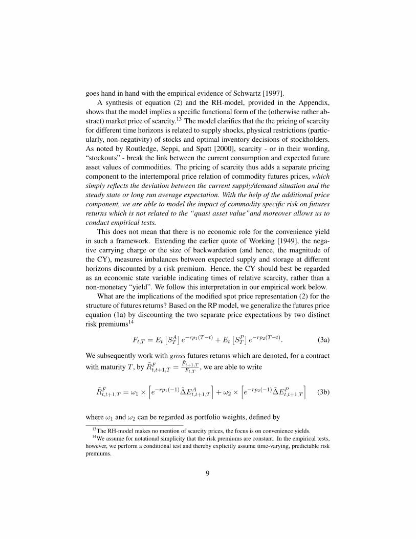
goes hand in hand with the empirical evidence of Schwartz [1997].A synthesis of equation (2) and the RH-model, provided in the Appendix,

shows that the model implies a specific functional form of the (otherwise rather ab-stract) market price of scarcity.13 The model clarifies that the the pricing of scarcityfor different time horizons is related to supply shocks, physical restrictions (partic-ularly, non-negativity) of stocks and optimal inventory decisions of stockholders.As noted by Routledge, Seppi, and Spatt [2000], scarcity - or in their wording,“stockouts” - break the link between the current consumption and expected futureasset values of commodities. The pricing of scarcity thus adds a separate pricingcomponent to the intertemporal price relation of commodity futures prices, whichsimply reflects the deviation between the current supply/demand situation and thesteady state or long run average expectation. With the help of the additional pricecomponent, we are able to model the impact of commodity specific risk on futuresreturns which is not related to the “quasi asset value”and moreover allows us toconduct empirical tests.

This does not mean that there is no economic role for the convenience yieldin such a framework. Extending the earlier quote of Working [1949], the nega-tive carrying charge or the size of backwardation (and hence, the magnitude ofthe CY), measures imbalances between expected supply and storage at differenthorizons discounted by a risk premium. Hence, the CY should best be regardedas an economic state variable indicating times of relative scarcity, rather than anon-monetary “yield”. We follow this interpretation in our empirical work below.

What are the implications of the modified spot price representation (2) for thestructure of futures returns? Based on the RP model, we generalize the futures priceequation (1a) by discounting the two separate price expectations by two distinctrisk premiums14

Ft,T = Et

[SAT

]e−rp1(T−t) + Et

[SPT

]e−rp2(T−t). (3a)

We subsequently work with gross futures returns which are denoted, for a contract

with maturity T , by RFt,t+1,T =

Ft+1,T

Ft,T, we are able to write

RFt,t+1,T = ω1 ×

[e−rp1(−1)∆EA

t,t+1,T

]+ ω2 ×

[e−rp2(−1)∆EP

t,t+1,T

](3b)

where ω1 and ω2 can be regarded as portfolio weights, defined by13The RH-model makes no mention of scarcity prices, the focus is on convenience yields.14We assume for notational simplicity that the risk premiums are constant. In the empirical tests,

however, we perform a conditional test and thereby explicitly assume time-varying, predictable riskpremiums.

9

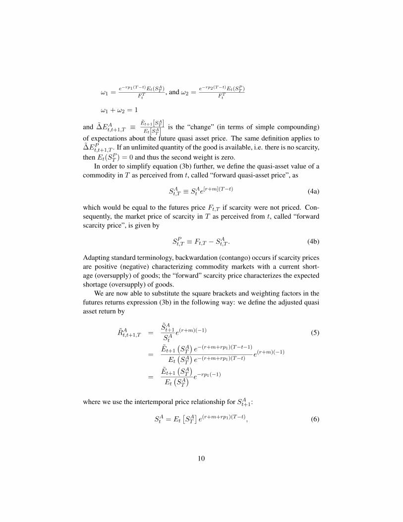
ω1 =e−rp1(T−t)Et(SAT )

FTt, and ω2 =

e−rp2(T−t)Et(SPT )

FTt

ω1 + ω2 = 1

and ∆EAt,t+1,T ≡

Et+1[SAT ]Et[SAT ]

is the “change” (in terms of simple compounding)

of expectations about the future quasi asset price. The same definition applies to∆EP

t,t+1,T . If an unlimited quantity of the good is available, i.e. there is no scarcity,then Et(S

PT ) = 0 and thus the second weight is zero.

In order to simplify equation (3b) further, we define the quasi-asset value of acommodity in T as perceived from t, called “forward quasi-asset price”, as

SAt,T ≡ SA

t e[r+m](T−t) (4a)

which would be equal to the futures price Ft,T if scarcity were not priced. Con-sequently, the market price of scarcity in T as perceived from t, called “forwardscarcity price”, is given by

SPt,T ≡ Ft,T − SA

t,T . (4b)

Adapting standard terminology, backwardation (contango) occurs if scarcity pricesare positive (negative) characterizing commodity markets with a current short-age (oversupply) of goods; the “forward” scarcity price characterizes the expectedshortage (oversupply) of goods.

We are now able to substitute the square brackets and weighting factors in thefutures returns expression (3b) in the following way: we define the adjusted quasiasset return by

RAt,t+1,T =

SAt+1

SAt

e(r+m)(−1) (5)

=Et+1

(SAT

)e−(r+m+rp1)(T−t−1)

Et

(SAT

)e−(r+m+rp1)(T−t)

e(r+m)(−1)

=Et+1

(SAT

)Et

(SAT

) e−rp1(−1)

where we use the intertemporal price relationship for SAt+1:

SAt = Et

[SAT

]e(r+m+rp1)(T−t), (6)

10

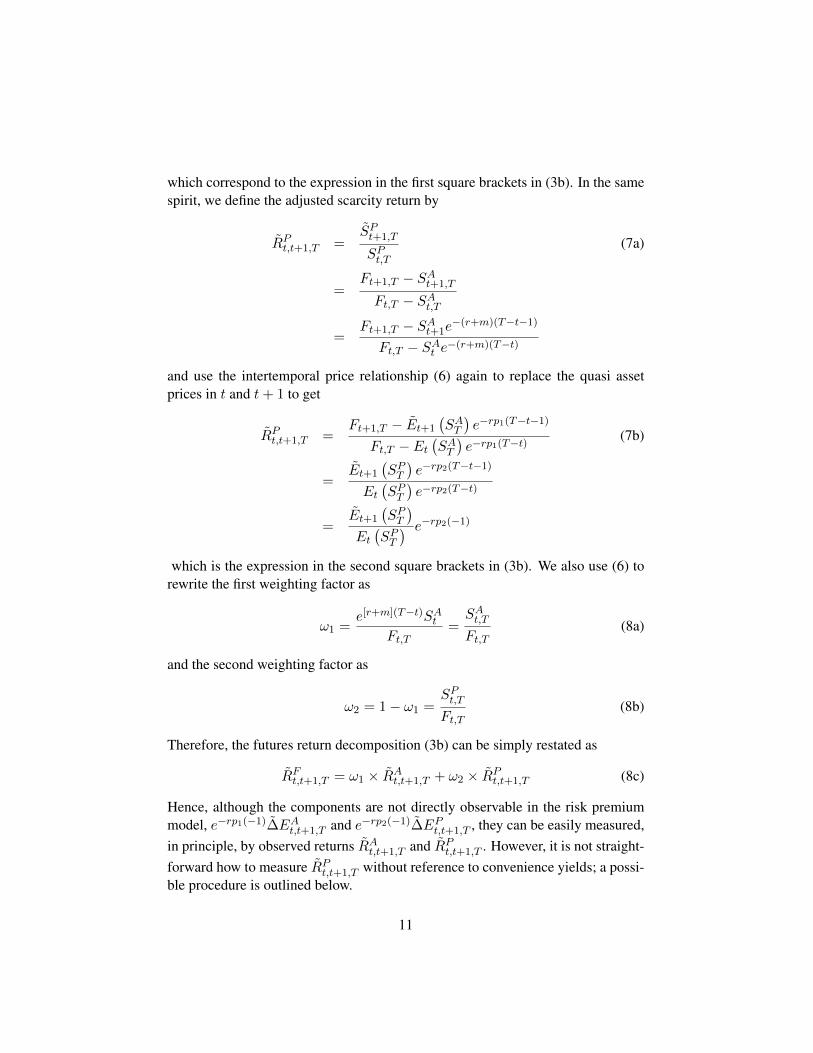
which correspond to the expression in the first square brackets in (3b). In the samespirit, we define the adjusted scarcity return by

RPt,t+1,T =

SPt+1,T

SPt,T

(7a)

=Ft+1,T − SA

t+1,T

Ft,T − SAt,T

=Ft+1,T − SA

t+1e−(r+m)(T−t−1)

Ft,T − SAt e−(r+m)(T−t)

and use the intertemporal price relationship (6) again to replace the quasi assetprices in t and t+ 1 to get

RPt,t+1,T =

Ft+1,T − Et+1

(SAT

)e−rp1(T−t−1)

Ft,T − Et

(SAT

)e−rp1(T−t)

(7b)

=Et+1

(SPT

)e−rp2(T−t−1)

Et

(SPT

)e−rp2(T−t)

=Et+1

(SPT

)Et

(SPT

) e−rp2(−1)

which is the expression in the second square brackets in (3b). We also use (6) torewrite the first weighting factor as

ω1 =e[r+m](T−t)SA

t

Ft,T=SAt,T

Ft,T(8a)

and the second weighting factor as

ω2 = 1− ω1 =SPt,T

Ft,T(8b)

Therefore, the futures return decomposition (3b) can be simply restated as

RFt,t+1,T = ω1 × RA

t,t+1,T + ω2 × RPt,t+1,T (8c)

Hence, although the components are not directly observable in the risk premiummodel, e−rp1(−1)∆EA

t,t+1,T and e−rp2(−1)∆EPt,t+1,T , they can be easily measured,

in principle, by observed returns RAt,t+1,T and RP

t,t+1,T . However, it is not straight-forward how to measure RP

t,t+1,T without reference to convenience yields; a possi-ble procedure is outlined below.

11

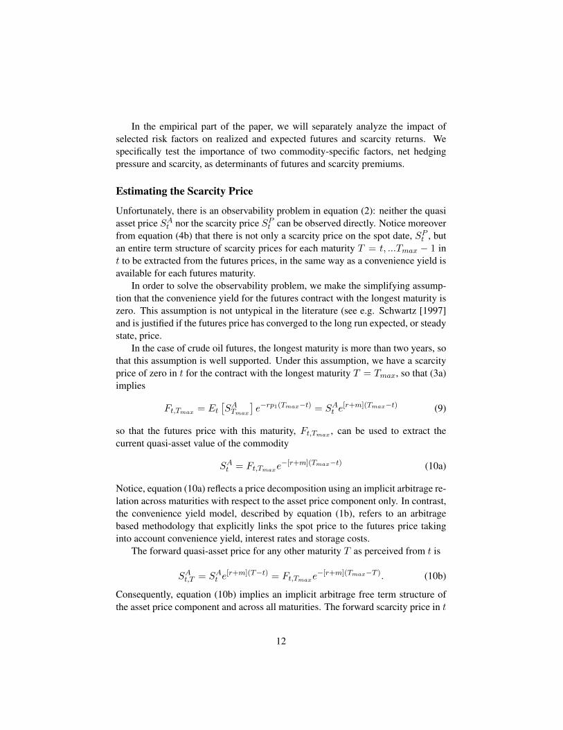
In the empirical part of the paper, we will separately analyze the impact ofselected risk factors on realized and expected futures and scarcity returns. Wespecifically test the importance of two commodity-specific factors, net hedgingpressure and scarcity, as determinants of futures and scarcity premiums.

Estimating the Scarcity Price

Unfortunately, there is an observability problem in equation (2): neither the quasiasset price SA

t nor the scarcity price SPt can be observed directly. Notice moreover

from equation (4b) that there is not only a scarcity price on the spot date, SPt , but

an entire term structure of scarcity prices for each maturity T = t, ...Tmax − 1 int to be extracted from the futures prices, in the same way as a convenience yield isavailable for each futures maturity.

In order to solve the observability problem, we make the simplifying assump-tion that the convenience yield for the futures contract with the longest maturity iszero. This assumption is not untypical in the literature (see e.g. Schwartz [1997]and is justified if the futures price has converged to the long run expected, or steadystate, price.

In the case of crude oil futures, the longest maturity is more than two years, sothat this assumption is well supported. Under this assumption, we have a scarcityprice of zero in t for the contract with the longest maturity T = Tmax, so that (3a)implies

Ft,Tmax = Et

[SATmax

]e−rp1(Tmax−t) = SA

t e[r+m](Tmax−t) (9)

so that the futures price with this maturity, Ft,Tmax , can be used to extract thecurrent quasi-asset value of the commodity

SAt = Ft,Tmaxe

−[r+m](Tmax−t) (10a)

Notice, equation (10a) reflects a price decomposition using an implicit arbitrage re-lation across maturities with respect to the asset price component only. In contrast,the convenience yield model, described by equation (1b), refers to an arbitragebased methodology that explicitly links the spot price to the futures price takinginto account convenience yield, interest rates and storage costs.

The forward quasi-asset price for any other maturity T as perceived from t is

SAt,T = SA

t e[r+m](T−t) = Ft,Tmaxe

−[r+m](Tmax−T ). (10b)

Consequently, equation (10b) implies an implicit arbitrage free term structure ofthe asset price component and across all maturities. The forward scarcity price in t

12

reflecting scarcity to be expected in T is the difference between (10b) the observedfutures price Ft,T ,

SPt,T = Ft,T − SA

t,T = Ft,T − Ft,Tmaxe−[r+m](Tmax−T ) (11)

The second equality shows that under our assumption the term structure of forwardscarcity prices, as estimated in t, can be directly derived from the observed termstructure of futures prices. Obviously, the spot scarcity price, SP

t,t ≡ SPt , is a spe-

cial case, SPt = Ft,T −SA

t . The quasi-asset return and scarcity-return componentscan then be calculated based on the equation (8c).

It may furthermore be helpful to notice that scarcity returns as defined here canbe computed as returns from a portfolio containing a long futures position withmaturity t (t ranging from the shortest to the second longest maturity) and a shortfutures position with maturity Tmax. Based on our assumption that the scarcityprice is zero for the longest maturity, this corresponds to a net long position in the“scarcity” of the underlying commodity.

Oil Price and Descriptive Statistics

Our empirical work is based on daily WTI crude Oil futures prices from NYMEXfor the period December 16, 1994 to December 17, 2010 to construct monthly ma-turity specific continuously compounded futures returns. All returns are denom-inated in US dollars. We only select maturities with a sufficiently high liquidity,which restricts the use of contracts at the longest end of the maturity spectrum. Formaturities up to 27 months, the average trading volume for each delivery month ismore than 65 million USD per trading day. For longer delivery only the deliverymonths June and December have adequate liquidity. We have finally selected 14contracts with maturities on average ranging from 1.1 to 27.0 months.

We implement a monthly roll-over strategy to construct log futures returns ona daily basis for the first 13 maturities, where contracts are rolled on the 10th busi-ness day of each month. Due to the poor liquidity of the available longer datedmaturities, a 6 months roll-over strategy is applied for the 14th maturity, whereasthe contracts are rolled on the 10th business day of June and December. Rolling re-turns between consecutive contracts is a widely-used methodology in the empiricalfutures market literature; see Gorton and Rouwenhorst [2006], and many others.The methodology provides rolling futures return series for the 1st nearby contract15

represented by the 1st maturity, the 2nd nearby contract stands for the second ma-turity and so on, up to the 13th maturity. Finally, the 14th maturity includes only

15The nearby contract denotes the futures contract with the next delivery respectively with theshortest time to delivery.

13

June and December contracts with an approximate time to delivery between 23.9and 30.1 months. The empirical tests are based on monthly returns which are time-aggregates of the daily log returns. However, a day-based monthly observationfrequency is not appropriate, due to the fact that most statistics are not publishedon the same day. As a consequence, the returns were aggregated from Friday toFriday either over four or five weeks depending on the week in which the monthlyreported statistics are released.16

Exhibit 5 shows in columns three to five the average, minimum and maximumtime to maturity in months of the contracts. Monthly return distributional char-acteristics are presented in columns six to ten and the market liquidity defined asthe average daily trading volume is given in the last column. Using the first ma-turity (row one) as an example, the average time to delivery is 1.1 months witha maximum of 1.7 months and a minimum of 0.4 months. The average monthlyreturn is 0.76% with a standard deviation of about 10.5%. Indeed, the well-knownSamuelson effect17, i.e. a monotonically decreasing volatility of futures returns forlonger maturities, can clearly be seen from these figures. Average returns increasefrom the 1st to the 6th maturity, and slightly fall for the longer maturities. The fig-ures presented in columns eight and nine indicate that the return distributions of allmaturities show a long left tail and are leptokurtic distributed in comparison to thenormal distribution. This picture is confirmed by the Jarque-Bera (J.B.)-test statis-tic of normality given in column ten. The last column shows the average tradingvolume on each trading day over the sample period. The highest trading activ-ity occurs in the contracts with shortest time to maturity, which is a well-knownfeature of derivative markets.

Exhibit 6 displays descriptive statistics of the scarcity prices as extracted fromthe term structure of futures prices based on equation (11) by ignoring the storagecosts due to a lack of reliable and representative data. As a result, the implicitweight of the scarcity price component is slightly lower as if storage costs areincluded. Neglecting storage costs may also be a problem if they are time varying;however, the variation is very small compared to the volatility of the futures returnsof crude oil.18 Notice that we have only 13 different maturities for the scarcity pricecompared to 14 for the future prices. We assume that the price of the 14th maturityhas no scarcity price component, so that we use that price as “quasi asset value”.As expected, scarcity prices decrease with increasing time to maturity, as well as dothe standard deviations shown in column two to five. Stationary tests are displayed

16For example, inventories and other commodity-specific statistics are reported in weekly cycleswhereas other economical reports are released once a month, like the U.S. Consumer Price Index(CPI). Therefore, the wording four to five weeks returns would be more precise, but inconvenient.

17See Samuelson [1965].18The zero cost assumption is typical in the empirical literature.

14

in columns six and seven. The Augmented Dickey-Fuller (ADF) and Phillips-Perron (PP) test statistics indicate that the null hypothesis of nonstationary can berejected for forward scarcity prices for all maturities at least on the 10% level. Thestatistical characteristics of scarcity returns for each maturity T , computed fromthe portfolio decomposition in equation (3b) or (7), are displayed in columns eightto twelve. Computations are based on riskfree rates proxied by one or two yearU.S. Treasury rates. The storage cost does not affect the scarcity returns as long asthey remain constant over the observation interval.

Not surprisingly, and reinforcing the Samuelson effect, the standard deviationof the scarcity returns is monotonically decreasing across the maturities, morestrongly than the standard deviations of futures returns. This observation indi-cates that the expected change about future scarcity, as revealed by the scarcityreturns, is a major determinant of the Samuelson effect. It strongly supports theobservation that the effect tends to be more pronounced in agricultural and energycommodities than in financial futures19, i.e. in commodities where storability islimited or costly.

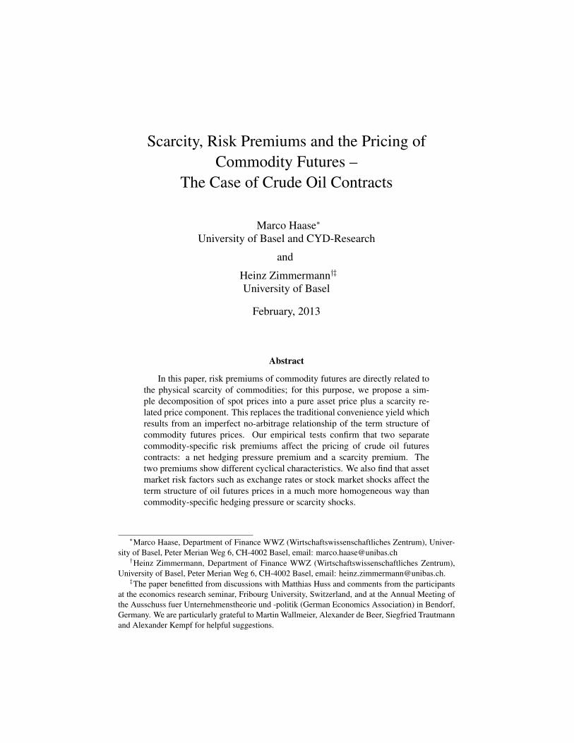
Illustrative time series of scarcity prices can be found in Exhibit 1. As notedearlier, time periods with positive (negative) prices are those where scarcity (sur-plus) of goods prevails and markets are in backwardation (contango). The graphreveals that time periods with scarcity in the oil market are substantially longerthan the time periods characterized by surplus. It also shows the high negativexscarcity prices during the recent financial crisis.

Empirical Tests

In this section, we test the hypothesis whether scarcity is a priced risk factor incrude oil futures contracts, and whether the pricing characteristics depend on thetime to maturity of the contracts. Our decomposition of futures returns into “quasiasset” and “scarcity” return components enables a more conclusive test of thishypothesis than other studies. We test the hypothesis whether the risk premiumof futures increases during times of relative scarcity; under the null hypothesis,scarcity-related risk factors should have a more substantial impact on the scarcityreturn component than on the overall futures returns. We add global risk factorsused in the asset pricing literature to investigate their impact on scarcity returnsand the overall futures returns.

We provide two sets of tests. First, a multifactor model is estimated for futuresand scarcity returns across 14 and 13 contract maturities respectively to analyze

19This is the conclusion of the study of Daal, Farhat, and Wei [2006] which investigates 61 com-modity futures covering a total of 6805 contracts.

15

the sensitivities of the returns with respect to the four risk factors. This is donein a multivariate regression framework. Second, a beta pricing model is estimatedusing GMM to empirically analyze the size and properties of the conditional factorrisk premiums, based on set of futures and scarcity returns.

Risk Factors

We include three global, asset-market related risk factors in our analysis (the USDexchange rate, the stock market and U.S. Consumer Price Index (CPI)) and twocommodity-related factors (net hedging pressure, and scarcity).Global Risk Factors

A natural choice for the the stock market risk are the excess returns on the S&P500 stock market index, denoted by ERSP

t . Obviously, we expect a positive riskpremium on the market factor. The currency risk factor, denoted by (∆FX), isproxied by Trade Weighted US Dollar Index which is published by Federal Reserve(FED). Oil in general is traded on worldwide markets and denominated in USD. Inthe sense that the USD can be regarded as a numeraire for international investorsin Crude Oil futures, the USD is a potentially priced risk factor. We expect that therisk premium is negatively related to the trade weighted USD index, due to the factthat an increase of the trade weighted USD reduces the real demand for oil in nonUSD currency-based countries. All used factors are available and published on aweekly basis at the end of the respective week (Friday).

It is not surprising that inflation is often associated with commodity pricechanges due to the fact that the U.S. Consumer Price Index (CPI) constitutes about40% commodities, see Erb and Harvey [2006]. Thus commodity futures are re-garded as a hedge against unexpected inflation.20 The U.S. CPI, provided by theFED, is used to measure the inflation rate and has the following form

IRt =CPIt − CPIt−1

CPIt−1

where IRt represents the inflation rate at time t. Based on the random walk model,the inflation today is the best predictor for future inflation. Following Chan, Chen,and Hsieh [1985] the unexpected inflation is defined as ∆IRt = IRt−IRt−1. Thedifferenced and de-meaned process is still autocorrelated until the fifth lag whichwere removed to get unexpected changes. On account of the inflation-hedge char-acteristics of commodity futures, a positive risk exposure is expected.Specific Risk Factors: Inventory Changes

20Note, only the unexpected innovations of inflation time series are pricing relevant, since expectedinflation is assumed to be factorized in asset prices.

16

Inventory levels are widely used as valid and immediately available proxy vari-ables for the stock-out risk of commodities. H. Working originally suggestedinventory levels to determine the cost of storage and futures prices; in subse-quent papers, e.g. Brennan [1958], the change (decrease) of inventories is re-garded as a valid indicator for scarcity. In recent studies, still both variables areused, but we follow the approach of a related paper Khan, Khokher, and Simin[2008] where withdrawals of stocks from storage are used.21 However, we switchsigns and define the log change of the seasonally adjusted inventories (INV ) as∆INVt ≡ log (INVt − INVt−1), so that a depletion of inventory, which prox-ies an increase of stock-out probability, has a negative sign. We expect a positiverisk premium for the change of the stock-out probability (i.e. a negative premiumassociated with ∆INVt), i.e. a high premium in times of relative scarcity.

Inventory data are available on a weekly basis from the United States Depart-ment of Energy (DOE). The data measure the Friday ending stocks in the US andare published by the DOE on Wednesday (10:30 am, Eastern Time) of the followingweek. As mentioned earlier, futures returns are based on Friday quotations. Thismatches the inventory data, but we have to take the publication lag properly intoaccount by relating the week t to the (published) week t+ 1 inventory changes.22.Specific Risk Factors: Net Hedging Pressure

The net hedging pressure captures the commodity market specific risk aversion; inmost empirical studies, e.g. de Roon, Nijman, and Veld [2000], it is measured by

NHPt ≡Nshort −Nlong

Nshort +N − long

where Nlong (Nshort) is the number of futures contracts bought (sold) by the com-mercial traders summarized over all traded WTI Crude Oil futures contracts onTuesday. If commercials are net short in futures (the backwardation case in theKeynes-Hicks theory), the ratio is positive, and negative otherwise. The data areavailable on a weekly basis from the Commodity Futures Trading Commission(CFTC); the information is collected on Tuesdays and published on Fridays. Thereport does not disclose which specific maturities were bought or sold. The levelof the hedging pressure time series is non-stationary; we therefore take first differ-ences

∆NHPt ≡ NHPt −NHPt−1

21The seasonally adjusted inventory time series are computed by implementing a seasonal decom-position procedure based on Loess.

22Khan, Khokher, and Simin [2008] find that the change of inventories has predictive power forWTI Crude Oil future returns. However, if we account for the publication lag, no statistically signif-icant predictive power remains.

17

to capture the innovations of the process. The differenced and de-meaned processis still autocorrelated, so that we remove the first three autocorrelations to get aseries with pure innovations.

We expect a positive reward for this risk factor: If e.g. in times of scarcity orotherwise surplus stock is reduced, hedging is expected to decrease (in accordancewith the classic theory of “speculative” stocks, Brennan 1958) and so should therisk premium earned by long speculators. Thus, a negative sign of ∆NHP isexpected to go in hand with a lower risk premium, hence the factor risk premiumshould be positive.

All time series of non-traded risk factors are de-meaned without other adjust-ments. Exhibit 7 Panel A gives a summary of the statistical characteristics of therisk factors. The Augumented Dickey-Fuller and the Phillips-Perron tests rejectthe null hypothesis of non-stationary for all factors at the 1% level.

Multivariate Regression Tests (SUR)

In a first step, we analyse the factor exposure of the futures and scarcity returnsacross contract maturities. The scarcity-related factor, as proxied by the changeof inventories, is of particular interest. We estimate the following multivariateregression equations for futures and scarcity returns, across all maturities:

rm,t = am + β′mft + εm,t (12)

m = 1...14 futures maturities; 1...13 scarcity maturities,

where rm,t denotes the futures (scarcity) return with the mth maturity and am de-notes the constant term. The (5 × 1) vector ft captures the unexpected monthlyfactor changes and the respective (5×1) vector of factor sensitivities is denoted byβm. Finally, εm,t represents the idiosyncratic component. Unlike similar studies(e.g. Khan, Khokher, and Simin [2008]), we do not estimate the equations for eachmaturity separately. In order to account for the cross-sectional correlation of resid-uals (which are substantial according to our non-reported results), we estimate asystem of equations by SUR (Seemingly unrelated regressions). The results for thefutures returns are summarized in Exhibit 8, for scarcity returns in Exhibit 9.Futures returns

The first column lists the maturity bucket of the contracts and the subsequentcolumns display the estimated regression coefficients with the t-test statistics notedin italics below. The last column contains the adjusted R-squared values. Con-sider, for example, the 5th maturity. The effect of scarcity (change of invento-ries (∆INV )) is significantly negative with a coefficient of -0.46 and a t-valueof -1.96; consistent with our hypothesis, the effect of withdrawals of inventories

18

(∆INV < 0), i.e. an increase in scarcity, increases futures returns on average.The coefficient related to the net hedging pressure (∆NHP ) is 0.92 and significantwith a t-value of 6.00. This corresponds to the standard risk premium explanationof expected futures returns where an increase in the short (long) hedging pressureincreases returns on long (short) futures positions.

Comparing the results across maturities provides the following insights: Thecoefficients related to scarcity are all negative and monotonically decrease (in ab-solute terms) for longer maturities, from -0.80 for the 1st maturity to -0.20 for thelongest maturity. The coefficients are all significant at least on the 95% level, ex-pect for the longest maturity. This result supports our hypothesis that inventorychanges has the highest impact on the contracts with immediately delivery and ismuch less important for the longest maturities. As a matter of fact, the longestcontract which we use to extract scarcity returns is insignificant, showing that therespective futures price reflects at most an asset value (as we assume).

The change of the hedging pressure (∆NHP ) is significant and positive acrossall maturities, but decreases from 1.20 (1th maturity) to 0.21 (14th maturity). Hence,the risk exposure of future returns to changes of the net hedging pressure is stronglypositive for short maturities and decreases gradually for longer maturities, also interm of statistical significance. Unfortunately, there are no maturity specific data todecompose the hedging pressure effect for individual maturities, but it can be as-sumed that most commercial hedging activities occur within the short maturities;in the case of crude oil, much of the short hedging pressure comes from “specu-lative” stockholders selling part of their inventory to hedge downside price risk.Since most of the capital of these investors is committed with a short time horizon,we would expect the observed maturity pattern of coefficients.

The stock market risk factor (ERSP ) is positive and significant for all matu-rities at least at the 5% level. The coefficients only slightly for longer maturities,from 0.28 (1st maturity) to 0.22 (14th maturity). The same finding applies to the thecurrency exposure (∆FX), which even shows weak decreasing behavior for longermaturities. It exhibits the expected negative sign for all maturities with highly sig-nificant coefficients for all contracts. Interestingly, the inflation risk factor (∆IR)is statistically significant at the 10% or 5% level only for contracts with a maturityof more than five months on average. The estimated coefficients show the expectedpositive sign, whereas the coefficient values increase with longer dated maturitiesfrom 3.00 (1th maturity) to 3.23 (14th maturity). The adjusted R-squared value ofthe equations ranges between 14.0% and 27.4%.

The most remarkable finding is that the asset market related factors affectthe futures returns in a much more homogeneous way across maturities than thecommodity-specific factors. To put it differently, asset market specific factors af-fect the term structure of futures prices in a much more parallel way than commodity-

19

specific factors. This has strong implications for the diversification potential ofcommodity futures for asset portfolios.

We run Wald tests to investigate the adequacy of the specified risk factors withrespect to our pricing tests. A valid risk factor should meet the following criteria(see Ferson and Harvey [1994]): The implied factor betas should be significantlydifferent from zero, and they should differ across maturities. Hence we test thenull hypotheses that the factor betas are jointly zero, and that they are equal acrosscontracts. The results in Exhibit 10 Panel A show that the first hypothesis cannot berejected for the inflation risk factors but four of the five predetermined factors showsignificant impact on WTI Crude Oil futures returns across maturities. The resultsof the second hypothesis, i.e. test of equality of betas, indicate that both commodityspecific risk factors help to explain return differences between contracts, whereastwo of the three global risk factors do not. In spite of the fact that the hypothesisof equality betas is rejected at the 5% level for the market risk factor (ERSP ) thenumerical values hardly differ from one another.Scarcity Returns

In the next step we estimate the same system of equation with the future returnsreplaced by scarcity returns from equation (8c). As noted earlier, scarcity pricescan only be constructed up to the 13th maturity. The results are displayed in Exhibit9. The betas for the commodity-specific risk factors decrease with longer maturi-ties, but are all highly significant. The sensitivities range from -0.57 to -0.16 forthe inventory factor, and from 0.98 to 0.25 for the net hedging pressure factor. Thecoefficients are only slightly smaller than for the futures returns, and their statisti-cal significance is of similar size. Interestingly, the hedging pressure effect is more(and highly) significant even at the long end of the term structure23.

The sensitivities for both financial market factors are numerically very smalland not significant. However, they show the expected signs. Like the financialfactors, the inflation risk factor is insignificant and the coefficients are close to zero.The estimated signs are negative up to the sixth maturity and positive afterwards.The R-squared value is in the same range as for the futures regression; the range isbetween 18.1% for the 13th maturity and 27.2% for the 3th maturity.

Wald Test Results

The results of the Wald tests are displayed in Exhibit 10 Panel B; all global riskfactor betas are jointly insignificantly different from zero, whereas the hypothesisof jointly zero betas can be rejected at the 1% level for all commodity specificrisk factor betas. Additionally, the Wald test statistics of hypothesis 2 indicate

23Notice when comparing the coefficients, that there are only 13 maturity buckets for the scarcityreturns.

20

that differences in the scarcity returns are explainable by commodity specific riskfactors.

Overall, the results suggest that almost the entire commodity-specific risk ex-posure (∆NHP and ∆INV ) of the futures is related to the scarcity price and notto the quasi asset price. While the risk structure with respect to the commodity re-lated factors depends on the time to maturity, the picture is totally different for theasset market related factors where the exposure is virtually the same for each ma-turity. Hence, the separation of return components reveals a remarkably differentrisk profile. With exception of the inflation factor, the Wald test results suggest thatthe predetermined risk factors significantly influence the WTI Crude Oil futuresand scarcity returns. Thus, the inflation risk factor is dropped from the subsequentexploration.

Conditional Beta Pricing Model Tests (GMM)

In this section we expand the multivariate regression model to a conditional betapricing model, i.e. an asset pricing model where expected futures returns are lin-early related to factor-betas and the associated expected factor risk premiums aretime-varying24. An asset pricing model imposes the restriction that the risk factorsare consistently priced across the contracts for the different maturities and therebyexclude arbitrage profits.

The general representation of a factor model discriminates between unexpectedfactor shocks common (systematic) to all assets, and specific shocks affecting in-dividual assets only:

ri,t = E [ri,t] +K∑j=1

βi,jδj,t + εi,t (13a)

i = 1, ..., N(assets,maturities), j = 1, ...,K(risk factors),

t = 1, ..., T

where ri,t represents the excess return25 on the i-th security observed over the pe-riod t−1 to t. The expected excess return isE [ri,t] and δj,t denotes the unexpectedchanges in the common risk factors, observed over the same period of time. Theβi,j are the asset specific exposures to the common risk factors. The asset specificor idiosyncratic return shocks are denoted by εi,t. In our setting, the asset universeis represented by N contract maturities included in the pricing test.

24This methodology is widely used in the empirical testing of asset pricing models; see Ferson[2003] for a methodological review.

25In the context of futures returns, excess returns are equal to returns.

21

The asset pricing model requires that expected returns are linearly related tothe factor risk premiums

E (ri,t | Ωt−1) =

K∑j=1

βi,jλj,t (Ωt−1) (13b)

i = 1, ..., N(assets,maturities), j = 1, ...,K(risk premiums),

where ri,t is the expected rate of return on asset i conditional on the informationset Ωt−1 available at the beginning of the measurement time interval, t − 1. Theexpected risk premium related to factor j is denoted by λj,t (Ωt−1). Apparently,we assume that the expected factor risk premiums may vary over time, while thebeta coefficients of the futures contracts are constant26.

Unfortunately the entire information set Ωt−1 is unobservable for the econo-metrician. We therefore make the common assumption that a set of global instru-mental variables Zt−1, which is a subset of Ωt−1, sufficiently mirrors the relevantconditional pricing information. We assume a total number of L − 1 instruments,such that for notational convenience a constant 1 can also be included in the (L×1)vector of instrumental variables Zt−1 in order to account for a time-invariant partof factor premiums. We assume a linear relationship between the vector of instru-ments and the expected factor j risk premium, λj,t:

λj,t (Zt−1) =

L∑v=1

ωj,vZv,t−1 (13c)

j = 1, ...,K(risk premiums), v = 1, ..., L(instruments)

where Zv,t−1 represents the v-th global information variable in t − 1. The ωj,v

capture the sensitivity of the j-th risk premium with respect to the v-th instrument.This approach allow us to compare the size, statistical significance and con-

ditional variation of the factor risk premiums implicit in the futures and scarcityreturns, and to derive conclusions about the relevance of these premiums, in partic-ular the premium related to scarcity, in the two price components. Moreover, thematurity structure of the factor sensitivities can be compared to the results from theSUR-regression, which provides a robustness-check for our findings in the previ-ous section.

26Empirical studies from asset markets, not including performance studies of actively managedfunds, demonstrate that the principal source of time-variation of expected returns on individual se-curities comes from the compensation of systematic risk, and to a much lesser extent from changingbetas. Of course, this need not necessarily hold for commodities. However, this issue is not addressedin this article.

22

Putting the specifications (13a), (13b) and (13c) together and using matrix no-tation, we get the following reduced form conditional asset pricing model:

rt = βωZt−1 + βδt + ut (14)

where rt denotes the (N ×1)-vector of period t continuously compounded futures,or scarcity, returns for the N maturity buckets. The variable Zt−1 denotes the(L×1)-vector of lagged instruments, indexed by t−1 for the time interval t; and δtdenotes the (K× 1)-vector of contemporaneous unexpected changes of the factorsin period t. Furthermore, ω is the (K ×L)-matrix of sensitivities of the factor riskpremiums with respect to the instruments; and β denotes the (N × K)-matrix offactor betas of theN futures maturities. The (N×1)-vector of idiosyncratic returncomponents is denoted by ut.

The equilibrium pricing model imposes the following restrictions on the cross-section of period-by-period futures returns across the N maturities: (i) The ω-coefficients are constrained to be equal across the maturities, and (ii) the interceptof the equations is assumed to be zero. The first restriction guarantees that theglobal factor prices are equal across maturities, which is, of course, an essentialfeature of a beta pricing model. Specifically, in the conditional setting, the con-straint on factor prices takes the form of constraints on matrix ω. The secondrestriction implies that there is no constant return component unrelated to factorrisk.Econometric SpecificationIn order to estimate the factor sensitivities and the conditional variation of the fac-tor risk premium simultaneously, we use the Generalized Methods of Moments(GMM) methodology with iterated weights and coefficients using Newey-Weststandard errors. GMM requires the specification of moment conditions which areconsistent with the equilibrium pricing model. However, we do not apply theseconditions directly to the residuals of equation (14) because the equation does notdiscriminate between traded and non-traded factors. For traded factors (such as theexcess return on the market) the risk premium need not to be estimated from thecross-section of assets, they can be directly determined from the average excessreturns. We thus add a “self-pricing” restriction for the traded assets 27. An addi-tional issue is related to the currency factor which is proxied by the Trade WeightedUS Dollar index (TWUSD) in the empirical analysis of the SUR test. Recall thatthe Wald test displayed in Exhibit 10 reveals that the currency factor betas are notsignificantly different across the contracts, which makes it impossible to estimatethe currency factor risk premium from the cross section of excess returns. This can

27This was recently recommended by Lewellen, Nagel, and Shanken [2010] and Jagannathan,Schaumburg, and Zhou [2010].

23

be accomplished by replacing the currency factor by the excess returns on a cur-rency mimicking portfolio28, which is a linear combination of the six constituentcurrencies with maximum squared correlation with the unexpected log changesof the TWUSD index.29 Like the risk premiums on the other traded factors, therisk premium on the currency factor is then estimated from the time series of themimicking currency excess returns.

Extending equation (14), two separate equations are specified for estimatingthe factor sensitivities and risk premiums; we exploit the fact that the relationshipbetween factors ft, unexpected factor shocks δt and factor risk premiums λ is givenbyE [rt − a− βft] = E[rt−β(λ+δt)] = 0, where ft = λ+δt, which permits anexact beta specification for traded and non-traded factors.30 Adding the self-pricingcondition of the traded factors gives the following system of residuals

εt =

e1,te2,te3,t

=

rt − (a+ βft)rt − βωZt−1fg,t − ωgZt−1

(15)

which is used to specify the orthogonality conditions below. The first equationis equivalent to a time-series regression for estimating the factor sensitivities (β-coefficients) and constant return components a. The second equation is derivedfrom the asset pricing restriction and is used to estimate the ω-coefficients, andtherefore the conditional risk premiums of the factors, from the time-series andthe cross-section of excess returns. Notice that ft represents the (K × 1) vectorof traded and non-traded factors, where the non-traded factors are mean-centeredwhile the traded factors are excess returns. The original currency factor (∆FX) isalways replaced by the mimicking portfolio returns (ERFX ). fg,t, a subset of ft,is a (Kg × 1)-vector of traded factors including the mimicking currency returns.Finally, ωg is the (Kg × L)-submatrix of ω and contains the sensitivities of thetraded factor risk premiums with respect to the instruments.

For deriving the GMM orthogonality conditions, we exploit the fact that theprediction errors (e2 and e3) are orthogonal to the set of instruments used to predictthe returns and traded factors. In contrast, the return residuals (e1) are orthogonalto the set of factors. We define an augmented (1 + K) × 1 vector Ft = [1 f ′t ]

′

28Notice that the currency factor itself is not a traded asset although the individual currencies are.29A key insight of modern asset pricing theory is that the pricing implications of mimicking factor

portfolios, i.e. factors projected onto the asset space, are the same as for the true non-traded factors.30See Kan and Zhou [1999] or Jagannathan and Wang [2002].

24

including a constant. The moment conditions are then

gT (a, β, ω) =

E (e1,t ⊗ Ft)E (e2,t ⊗ Zt−1)E (e3,t ⊗ Zt−1)

=

000

(16)

Notice that the ωg coefficients are estimated from the cross-section as well asfrom the time-series of the traded factors. However, GMM will put more weighton the time-series regression since the estimated factor risk premium on itself pro-duces the lowest residual variance.

The set of risk factors (f ) consists of two traded (ERSP and ERFX ) and twonon-traded factors (∆NHP and ∆INV ). The currency weights of the mimickingcurrency portfolio are estimated from a linear regression of the unexpected logchanges of the TWUSD index on six forward exchange rate returns with one monthto maturity. The selected currencies are the Australian dollar (AUD), Canadiandollar (CAD), Swiss franc (CHF), Euro (EUR), British pound (GBP), and JapaneseYen (JPY), all computed with respect to the USD.31

Due to the well-known limitations of GMM-systems, we cannot include allcontracts (maturites) in our estimation, which would imply 159 parameters with150 overidentifying restrictions to be estimated. Our selection of contracts relieson the following considerations: In order to identify risk premiums from the crosssection, it is important that the betas vary across the futures and scarcity returns.However, the differences of commodity specific factor betas between successivematurities are small. We therefore include only five futures maturities with a min-imum maturity gap of three months in our GMM system. Because the scarcityreturns are computed from futures returns, the five specified futures maturities areexcluded for the selection of scarcity returns. This procedure prevents multipleusage of the same return information inherent in a specific maturity. Moreover,since a high correlation between scarcity returns with similar maturities exists,only three maturities with a minimum gap of five months are included. Hence, ourreturn space contains four futures returns with maturities of 1, 5, 9 and 14 months,and three scarcity returns with maturities of 3, 7 and 11 months.

Our GMM system therefore includes N = 7 returns, K = 4 risk factors andL = 6 instruments including the constant. There are 1×N intercepts plus K ×Nbeta coefficients to be estimated, andK×L omega coefficients, i.e. a total numberof N + K × (N + L) parameters. On the other hand, the pricing model impliesN × (1 + K + L) moment restrictions related to returns and Kg × L moment

31The squared correlation between the original currency factor and the factor mimicking returns is98%. Notice that ERSP is included as an additional exogenous variable in the mimicking portfolioregression.

25

restrictions related to traded factors. For N = 7, this gives 59 parameters to beestimated and 89 moment conditions, leaving 30 overidentifying restrictions.Conditioning Information: Instrumental Variables

The set of lagged instrumental variables which are used to characterize time-varyingexpectations includes four financial and one commodity-related instruments. Theidea in specifying adequate instruments is to exploit priced information in the fi-nancial or commodities markets observed in the term structure of rates, prices,spreads, yields, ratios, and others. For stock and bond markets, adequate instru-ments have been analyzed by Fama and French [1989], Ferson and Harvey [1993]and others, while in the commodity futures pricing literature the studies of Young[1991], Bjornson and Carter [1997] and Khan, Khokher, and Simin [2008] use as-set market related and commodity-specific conditioning information. Based on thisliterature, we specify four instruments from securities markets and one commodity-specific instrument.

Financial instruments capture conditioning information related to the cyclicityof business conditions. The first variable is the TED spread (TED) defined as thedifference between the 3-months Eurodollar rate and the 90-day yield on US Trea-sury bills; the spread is regarded as an indicator of disruption in the internationalfinancial system and the state of global liquidity. The spread is used in the assetpricing literature (e.g. Fama and French [1989] or Ferson and Harvey [1993]) aswell as in commodity futures studies (e.g. Young [1991]). The second financialinstrument, the term spread (TS), is the slope of the US term structure of interestrates which is widely used as a predictor of the state of the economy. The termspread is constructed as difference between the two-year US Treasury-bond rateand three months US Treasury bill rate. The third financial instrument is the priceearnings ratio of the S&P 500 Index (PE), defined as the total market capitaliza-tion divided by the total earnings per year. A high ratio is typically associated,with given standard dividend or earnings discount models of the stock market, lowexpected returns or high expected growth rates of dividends or earnings and thuswith favorable economic perspectives. The last financial instrument is the creditspread (CS) which is widely regarded as indicator of global risk aversion. We usethe a log yield spread between BBB corporate bonds and US Treasuries with a 2year maturity. All financial instruments are downloaded from Thomson ReutersDatastream (the respective series codes are available upon request).

The last instrument is the slope of the commodity specific term structure (CTS)as extracted from the Crude Oil futures price over the first year. Fama and French[1987] were among the first to predict futures prices changes using the slope of theforward curve. Other papers test excess returns from tactical strategies of portfo-lios with long positions in backwardated commodity futures and short positions in

26

contangoed futures, see e.g. Gorton and Rouwenhorst [2006], Gorton, Hayashi,and Rouwenhorst [2008] as well as by Erb and Harvey (2006). In our interpreta-tion of the slope of the commodity term structure, we follow the interpretation ofWorking [1949] that a negative price of storage occurs when supplies are relativelyscarce. Based on the heterogeneity in the risk aversion of speculative or produc-tive storage holders, our model requires a higher stock-out related risk premium inperiods of scarcity (low inventories), whereas the risk premium based on hedgingactivity decreases when inventories are low. We measure the slope of the futuresprice structure inversely (i.e. positive values for backwardation)32 according tocts = ln

(Ft1Ft2

)where Ft1 and Ft2 are the futures prices of the first maturity and

the maturity one year ahead.Summary statistics of the instrumental variables are displayed in Exhibit 7

Panel B. The time series are de-meaned and standardized by their respective stan-dard deviation. This makes it easier to compare the impact of the instruments onthe various risk premiums.Empirical Results

The results of the conditional model are displayed in Exhibit 11. Panel A shows theGMM estimation results of the beta coefficients, i.e. the estimated sensitivities ofthe futures and scarcity returns to the risk factors. The overall results are very closeto those in the multivariate regression analysis. The risk exposure to changes of thenet hedging pressure (∆NHP ) is positive and significant across all maturities. Therisk exposure to the changes in the probability of stock-out (∆INV ) is negativeand significant across all maturities. In both cases, the absolute value of the coeffi-cients decrease for longer maturities. As in the multivariate regressions, the effectof the asset market factors (ERSP and ERFX ) is much more homogeneous acrossfutures maturities and close to zero for all scarcity returns.

Exhibit 11 panel B displays the GMM estimates of the ω-coefficients whichdescribe the relation between the risk factors (rows) to the lagged conditioning in-struments (columns). Among the asset market instruments, the PE-ratio seems tobe the most important; it significantly affects net hedging pressure. A higher ratio(which typically signals favourable economic perspectives) increases the hedgingpressure related risk premium. Taking the positive sign of the hedging related fac-tor exposure into account, this implies that a higher PE-ratio increases forecastedfutures returns. Likewise, the term spread (TS) has a significant and positive im-pact, but only on the hedging pressure risk premium. This result indicates that onthe hedging activity related risk premium increases during times of a prosperingeconomy.

32This facilitates comparison with the empirical papers using the convenience yield as explanatoryor exogenous variable for futures returns.

27

More interestingly, both the ∆NHP premium as well as the ∆INV premiumare significantly related to the slope of the futures curve (CTS). This means thatin times of relative scarcity, as indicated by an inverse term structure of the fu-tures prices, the scarcity premium increases and the net hedging pressure premiumdecreases. A numerical example illustrates this: Assume that the term structuregets more backwardated by one standard deviation. When taking the beta andomega coefficients in Exhibit 11 into account, the effect on the monthly risk pre-mium of ∆INV is (−0.65)× (−0.028) = 1.8% for the first futures maturity. Forthe same futures maturity, the effect on the monthly risk premium of ∆NHP is(1.17) × (−0.010) = −1.2%. The overall premium would only change slightlyby 0.6% but the distinction occurs in the composition of the premium! A visualinspection of the dynamics and composition of the conditional futures risk pre-mium confirms the often countercyclical behavior of the two components33. Theresults strongly confirm the hypothesis that two separate risk premiums influencethe pricing of futures contracts, and that their impact depends on the commodityspecific state of scarcity and on the overall economic conditions. The last columnof Exhibit 11 displays the mean pricing error (MPE) for all future and scarcity re-turns. Interestingly, the MPE is negative for the shortest and positive for longerdated futures maturities and the MPE’s for scarcity returns are lower than for fu-tures returns. Overall, the model mean absolute pricing error (MAPE) across allfutures, scarcity prices and traded factors is 15 basis points per month, displayedat the bottom of Exhibit 11.

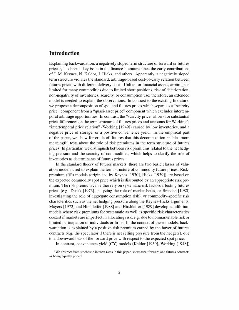
With respect to the goodness of fit of the model, J-test statistic indicates thatthe model restrictions cannot be rejected. The chi-square statistic is 23.1 with ap-value of 0.95 for 30 degrees of freedom. In order to visualize the size of theimplied pricing errors (α’s) generated by the pricing model, the predicted meanexcess returns on the assets are plotted against the actual mean excess returns inExhibit 2. The magnitude of the pricing error is reflected by the deviation of theassets from the 45 line. The returns on the four futures maturities are located inthe upper right area of the diagram, whereas the three scarcity returns are locatedin the middle. Obviously, the model underestimates the actual returns for all fu-tures contracts except the shortest maturity which is overestimated by 0.25%. Incontrast, the scarcity and traded factor returns are close to the 45 line. In spiteof the J-test which is unable to reject the model restrictions, the average deviationfrom the 45 line is 9 basis points per month or 1.1% per year, indicating that thepricing model still has a potential for improvement.Time Series of Conditional Risk Premiums

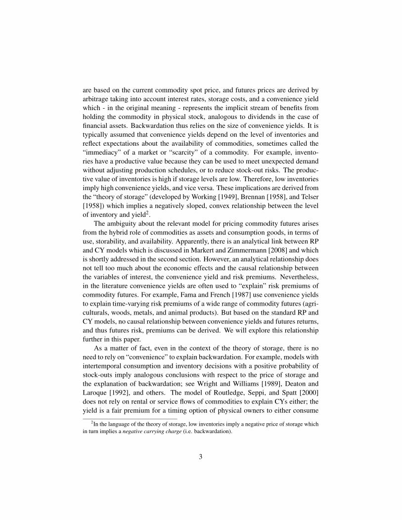
Exhibit 3 provides an illustrative decomposition of the expected futures premium33The correlation coefficient between both commodity specific risk factor premiums is only 0.25.

28

for the shortest (Panel A) and longest maturity (Panel B). The time series showthe relative impact of the four priced risk factors on the overall premium. In ac-cordance to the empirical results, the scarcity (gray) and hedging (light gray) riskpremiums indicate a countercyclical behavior, but the impact on the 14th maturityis obviously much lower and close to zero for the hedging risk premium; see PanelB. In contrast, the currency and market risk premiums exhibit a more unidirectionalbehavior with approximately the same effect for the longest and shortest maturities.

A key insight is that the futures contract with the longest maturity used (14th)shows little exposure to scarcity related risk, i.e. the beta of 0.32 obtained fromthe GMM estimation is slightly higher than the beta of 0.2 obtained from the SURestimation. The result does not necessarily contradict our hypothesis that there isno commodity specific impact on the asset price component, it rather indicates thatthe 14th maturity is not a perfect proxy for the steady state price.

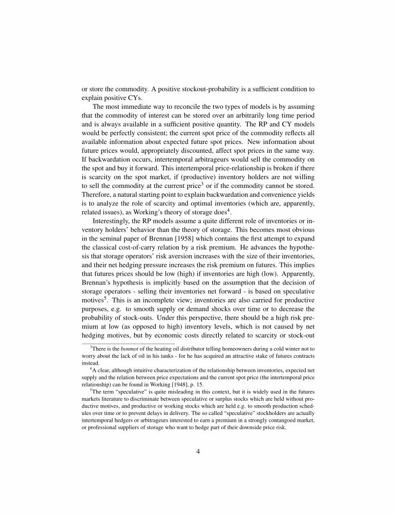
Comparing the decomposition of the expected scarcity price risk premiumsfor the 3th (Panel A) and 11th maturity (Panel B), as displayed in Exhibit 4, con-firms our hypothesis that only commodity specific risk premiums affect the scarcityprice, whereas the impact of market related risk premiums are marginal. Thescarcity and hedging premium displays the same cyclical pattern as for the futuresreturns.34

Robustness and Stability Tests: Summary Findings

Several robustness tests are performed.35 First, larger sample sizes increase the pre-cision of parameter estimates. We therefore replicate the estimation with weeklyinstead of monthly data over the same period, which increases the sample size con-siderably. Second, we specify different subperiods to test for stability over time,which comes at cost of smaller sample sizes and potential dilution of long termbusiness cycle information, which are particularly important in a conditional esti-mation framework. On the other hand, it could be argued that the empirical resultsmay be distorted by the financial crises in 2008. Therefore, this particular period isexcluded and the data sample is cutoff by the end of 2007, which reduces the num-ber of observations to 156. Third, we replace the change in inventories as a scarcityrelated risk factor with the change of the so called “forward demand cover”36. Fi-nally, in order to test the impact of additional, sector related systematic risk factors,we substitute the market risk factor, previously proxied by the S&P 500 Index, with

34The scaling factor is the same for Exhibit 3 and 4.35Due to space limitations, the results are not displayed here. They are available on request from

the authors.36This particular variable and its construction is explained in the documents provided by the De-

partment of Energy.

29

the S&P 600 Energy Index. The index comprises the firms in the energy sector aspart of the S&P 600 Small Cap index.

Our overall finding is that the results remain qualitatively stable. The onlynoteworthy exception occurs when the recent financial crisis is excluded from thesample period: While the impact of the global risk factors is still homogeneousacross the futures maturities, the quantitative effects are much smaller (about halffor the currency risk factor, and close to zero for the remaining two factors). How-ever, the the effects are virtually unchanged for the two specific risk factors (nethedging pressure and inventory shocks).

Conclusions

The pricing of commodity futures is challenged by the fact that many commodi-ties share the features of consumption or production goods and investment as-sets. As the current backwardation cycle in silver futures demonstrates, thesecharacteristics are not even constant over time. This dual nature of commodityderivatives was a key characteristic of the commodity pricing theory from the verybeginnings in the 30s of the last century, which is best reflected in the Keynes-Hicks risk-premium/hedging-pressure approach compared to the Kaldor-Workingconvenience-yield-theory-of-storage approach. Unfortunately it is difficult to rec-oncile the two approaches if markets are incomplete. Arbitrage strategies are in-validated due to scarcity or limited storability of goods. While the notion of “con-venience yield” has from the beginning been widely used to characterize the dis-tinctive features of commodity futures and remains popular today, its economicmeaning is somehow obscure.

We prefer an approach which strictly separates between a quasi asset pricecomponent which excludes intertemporal arbitrage, and an additional “scarcity”(or maturity-specific or incomplete markets) related price component, much in thespirit of Working (1948). This makes it possible to separate out asset related andcommodity-specific risk factors and to test whether they impact the two price com-ponents separately. Commodity-specific risk components are related to the changein the stock-out probability, measured by inventory changes, and hedging pressure- both factors are related to scarcity, but with different sign. Our empirical resultsshow, indeed, that both risk components co-exist and exhibit distinctive cyclicalproperties based on the heterogeneity in the risk aversion of speculative and pro-ductive motivated inventory holders. We also find that asset market risk factorssuch as exchange rates or stock market shocks affect the term structure of futuresprices in a much more homogeneous way than commodity-specific hedging pres-sure or inventory shocks.

30

Our findings have a wide range of implications beyond those addressed inthis paper. For example, the attractiveness of commodity investments is seen inthe low correlations vis-a-vis stocks, bonds and currencies. Our results show thatthe low correlations rely almost exclusively on the “scarcity” price component ofWTI Crude Oil futures. This gives some guidance which commodities should beselected for diversification purposes by securities markets investors. Moreover,the results clarify some topics of general interest related to recent criticism aboutspeculative pressure of commodity speculation. Do long only investors of futurescontracts push cash prices upwards? This argument would be valid if speculatorswould physically store commodities and carry it forward. This is not the typical be-havior of speculators. If this would prevail, we should observe a rising futures termstructure and rising inventories. But this is not what we observe: our results indi-cate a negative contemporaneous relation between inventory changes and nearbyfutures returns. Speculation is unlikely to be the source of the price disturbanceson the commodities markets, at least not for crude oil.

31

Outline and synthesis with the Ribeiro and Hodges [2004]Model

The model of Ribeiro and Hodges (RH) provides a valuable economic frameworkfor our separation of quasi-asset value and scarcity price. A key feature of the RH-model is that the dynamics of futures prices for a storable commodity is derivedfrom the interaction between exogenous (net) supply shocks of the commodityand endogenous (optimal) inventory decisions of agents. This framework allows itto analyze equilibrium price expectations, forward curves and convenience yieldswithin an optimizing framework, to analyze the effect of inventory levels or supplyshocks, and in particular, to investigate how spot and forward prices are related tothe steady state storage policy implied by the model. This is a particular importantimplication of the model because it provides a direct link to our specification inequation (10a).

The most important elements of the model are outlined here: The rate of supplyis modeled by an Orenstein-Uhlbeck process

dzt = α (z − zt) dt+ σdBt (.17)

where z is the supply level, dz the supply rate, α is the speed of mean reversion, zis the long run mean supply level at which z converges as t goes to infinity, σ is theconstant volatility and Bt is a standard Wiener process. The endogenous storagelevel s satisfies

ds = u (s, z, t) dt, s ≥ 0 (.18)

where u represents the rate of storage which is also the decision variable in themodel. The decision about u depends on the actual amount in storage st and theexogenous supply zt. An additional constraint to be satisfied is b > 0, and theinventory level St must satisfy

0 ≤ st ≤ b (.19)

since negative storage is not allowed. The rate of supply must not exceed thestorage rate

ut ≤ zt. (.20)

The equilibrum condition that the quantity consumed q equals supply minus changeof storage

q = z − u (.21)

determines the spot market price of the commodity, characterized by the inverse de-mand function p (q), where ∂p

∂q < 0. To derivate the optimal storage rate u∗ (st, zt)at each state, the authors solve a standard dynamic optimization problem in con-tinuous time. They maximize the present value of an expected flow of profits; the

32

instantaneous profit rate is determined by the revenues from sales from storageminus the costs of holding the current stocks. The Bellman condition implies anoptimal storage rate u∗ (st, zt). Specifically, a linear price function

p (qt) = p (zt − ut) = a− b (zt − ut) (.22)

yields an optimal storage rate given by

u∗ (st, zt) =V ∗s + bzt − a

2b. (.23)

which is determined by the actual supply rate, the actual storage level and themaximized value function. The expected spot price in t for time T is

Et [pT ] = Et [a− b (zT − u∗T )] (.24)

The steady state conditions imply a long run price expectation of

Et [pT ] = a− bz (.25)

Notice that the Ribeiro and Hodges model assumes risk neutrality, so that priceexpectations are identical to futures prices. Therefore, the last equation implies thatin the long run, i.e. in the steady state, the futures price contains no convenienceyield - or in our terminology, that the scarcity price component of the “longest”contract is zero, provided that the maturity is sufficiently long.

Synthesis: A Characterization of Scarcity Prices

There is a natural link between our representation of scarcity prices and the Ribeiroand Hodges equilibrium model. Adapting their linear spot price equation and tak-ing conditional expectations in t, we get

Et

[SCT

]= Et [a− b (zT − u∗T )] (.26)

where a is a constant, b is the inventory capacity, zT is the supply level in T ,and u∗T = u∗ (sT , zT ) is the optimal storage rate in T . Replacing SC

T in the riskpremium model as of equation (1a), the futures price becomes

Ft,T = Et

[SCT

]e−rp(T−t) = Et [a− b (zT − u∗T )] e−rp(T−t), (.27)

The steady state implications of the Hodges and Ribeira model are

Et [zT→∞] = z (.28)

33

Et [u∗T→∞] = 0 (.29)

The implied steady state price expectation

Et

[SCT→∞

]= a− bz (.30)

can be used to re-express Ft,Tmax , the futures price with maximum available matu-rity which is used to estimate the quasi-asset price. We assume that maturity Tmax

is sufficiently long to be regarded as the steady-state time horizon, i.e.

Et [zTmax ] = z (.31)

Et

[SCTmax

]= a− bz (.32)

The implied futures price is then

Ft,Tmax = Et

[SCTmax

]e−rp(T−t) = [a− bz] e−rp(T−t), (.33)

Based on equation (10a) the spot quasi-asset price can be written as

SAt = Ft,Tmaxe

−[r+m](Tmax−t) = [a− bz] e−[r+rp+m](Tmax−t) (.34)

which is the expected steady-state spot price discounted by the risk and storage-cost adjusted discount rate (the risk premium is from equation (1a))37. The forwardquasi-asset price for maturity T as perceived from t is accordingly

SAt,T = Ft,Tmaxe

−[r+m](Tmax−T ) = [a− bz] e−rp(Tmax−t)e−[r+m](Tmax−T ) (.35)

Based on this, the current market price of “scarcity” as of equation (11) can bewritten as

SPt = SC

t − SAt (.36a)

= a− b (zt − u∗t )− [a− bz] e−[r+rp+m](Tmax−t)

= K + bze−[r+rp+m](Tmax−t) − (zt − u∗t )

where K is a level parameter determined by a and the discount factor. Hence, the

37To simplify the analysis, and without loss of insight, we do not differentiate between the assetand scarcity risk premium here. For the longest maturity contract, rp can be substituted by rp2 fromequation (3a).

34

“market price of scarcity” is positive - or the term structure is in backwardation -if the actual supply rate zt minus storage rate u∗t is less than the discounted steadystate, or expected long run, supply rate. If the actual supply rate minus storage rateexceeds the long run supply rate, our equation predicts a negative “market priceof scarcity” or a term structure in contango. The economic explanations is thatthere is either no storage capacity left (b = 1) or the commodity is not storable,like electricity or soy meal. The forward “market price of scarcity” from equation(11) is finally

SPt,T = Ft,T − SA

t,T = Ft,T − Ft,Tmaxe−[r+m](Tmax−T ) (.36b)

= a− bEt [zT − u∗T ] e−rp(T−t)

− [a− bz] e−rp(Tmax−t)e−[r+m](Tmax−T )

= K ′ + bze−[r+rp+m](Tmax−T ) − Et (zT − u∗T )

e−rp(T−t)

whereK ′ is again a level parameter determined by a and the discount factor. Again,the forward “market price of scarcity” is positive (negative) if the expected supplyrate zT minus optimal storage rate u∗T is less (more) than the discounted steadystate (expected long run) supply rate.

Of course, the pure arbitrage relation which characterizes classical the assetpricing setting can be thought as a special case in which the optimal storage rateu∗ is able to balance out intertemporal supply and demand in every state. Theoutstanding quantity of financial assets is fixed, there are no limits to storage, andmost financial assets are regarded as perfect substitutes (in a CAPM or APT world).

Moreover, this result helps to clarify the economical distinction between mod-eling a scarcity price and the convenience yield. CY-models try to explain theobserved futures prices by the current spot price with the help of an arbitrage re-lation taking into account storage and capital costs. The resulting deviation fromthis arbitrage free relation is described as an non monetary reward, namely the con-venience yield. With the help of the CY the arbitrage relation is always fulfilled.In contrast the developed extended valuation model does not require an arbitragefree relation between the spot and futures prices. The spot price is completelydetermined by physical supply and demand, whereas futures prices reflecting theexpected supply and demand situation for the spot price at the time of expiration.

35

References

BJORNSON, B., AND C. A. CARTER (1997): “New Evidence on Agriculture Com-modity Return Performance under Time-Varying Risk,” American AgriculturalEconomics, 79(3), 918–930.

BLINDER, A. S., AND L. J. MACCINI (1991): “Taking Stock: A Critical Assess-ment of Research on Inventories,” The Journal of Economic Perspectives, 5(1),73–96.

BREEDEN, D. T. (1980): “Consumption Risk in Futures Markets,” The Journal ofFinance, 35(2), 503–520.

BRENNAN, M. J. (1958): “The Supply of Storage,” The American Economic Re-view, 48(1), 50–72.

CHAN, K., N. CHEN, AND D. A. HSIEH (1985): “An Exploratory Investigation ofthe Firm Size Effect,” Journal of Financial Economics, 14, 451–471.

DAAL, E., J. FARHAT, AND P. P. WEI (2006): “Does futures exhibit maturityeffect? New evidence from an extensive set of US and foreign futures contracts,”Review of Financial Economics, 15, 113–128.

DE ROON, F. A., T. E. NIJMAN, AND C. VELD (2000): “Hedging Pressure Effectsin Future Markets,” The Journal of Finance, 55(3), 1437–1456.

DEATON, A., AND G. LAROQUE (1992): “On the Behaviour of CommodityPrices,” The Review of Economic Studies, 59(1), 1–23.

DUSAK, K. (1973): “Futures Trading and Investor Returns: An Investigation ofCommodity Market Risk Premiums,” The Journal of Political Economy, 81(6),1387–1406.

EASTHAM, J. K. (1939): “Commodity Stocks and Prices,” The Review of Eco-nomic Studies, 6(2), 100–110.

ERB, C. B., AND C. R. HARVEY (2006): “The Strategic and Tactical Value ofCommodity Futures,” Financial Analysts Journal, 62(2), 69–97.

FAMA, E. F., AND K. R. FRENCH (1987): “Commodity Futures Prices: Some Ev-idence on Forecast Power, Premiums, and the Theory of Storage,” The Journalof Business, 60(1), 55–73.

(1989): “Business conditions and expected returns on stocks and bonds,”Journal of Financial Economics, 25(1), 23–49.

36

FERSON, W. E. (2003): “Tests of multifactor pricing models, volatility boundsand portfolio performance,” in Handbook of the Economics of Finance, ed. byG. Constantinides, M. Harris, and R. Stulz, pp. 741–800. Elsevier.

FERSON, W. E., AND C. R. HARVEY (1993): “The Risk and Predictability ofInternational Equity Returns,” The Review of Financial Studies, 6(3), 527–566.

(1994): “Sources of risk and expected returns in global equity markets,”Journal of Banking and Finance, 18, 775–803.

GORTON, G., F. HAYASHI, AND G. ROUWENHORST (2008): “The Fundamentalsof Commodity Futures Returns,” Working Paper.

GORTON, G., AND K. G. ROUWENHORST (2006): “Facts and Fantasies aboutCommodity Futures,” Financial Analysts Journal, 62(2), 47–68.

HICKS, J. (1939): “Value and Capital,” .

HIRSHLEIFER, D. (1988): “Residual Risk, Trading Costs, and Commodity FuturesRisk Premia,” The Review of Financial Studies, 1(2), 173–193.

(1989): “Determinants of Hedging and Risk Premia in Commodity Fu-tures Markets,” Journal of Financial and Quantitative Analysis, 24(3), 310–331.

JAGANNATHAN, R., E. SCHAUMBURG, AND G. ZHOU (2010): “Cross-SectionalAsset Pricing Tests,” Annual Review of Financial Economics, 2, 49–74.

JAGANNATHAN, R., AND Z. WANG (2002): “Empirical Evaluation of Asset-Pricing Models: A Comparison of the SDF and Beta Methods,” The Journalof Finance, 57(5), 2337–2367.

KALDOR, N. (1939): “Speculation and Economic Stability,” The Review of Eco-nomic Studies, 7(1), 1–27.

KAN, R., AND G. ZHOU (1999): “A Critique of the Stochastic Discount FactorMethodology,” The Journal of Finance, 54(4), 1221–1248.

KEYNES, J. (1930): A Treatise on Money, vol. 2. Macmillan, London.

KHAN, S., Z. KHOKHER, AND T. SIMIN (2008): “Expected Commodity FuturesReturns,” Workingpaper.

LEWELLEN, J., S. NAGEL, AND J. SHANKEN (2010): “A skeptical appraisal ofasset pricing tests,” Journal of Financial Economics, 96(2), 175–194.

37

MARKERT, V., AND H. ZIMMERMANN (2008): “The Relationship between Risk-Premium and Convenience-Yield Models,” in Handbook of Commodity Invest-mensts, ed. by F. Fabozzi, R. Fuess, and D. G. Kaiser, pp. 113–143. John Wi-ley&Sons.

MAYERS, D. (1972): “Nonmarketable Assets and Capital Market Equilibrium un-der Uncertainty,” in Studies in the theory of capital markets, ed. by M. Jensen,pp. 223–248. New York: Praeger.

PINDYCK, R. S. (1994): “Inventories and the Short-Run Dynamics of CommodityPrices,” The RAND Journal of Economics, 25(1), 141–159.

RIBEIRO, D. R., AND S. D. HODGES (2004): “Equilibrium Model for CommodityPrices: Competitive and Monopolistic Markets,” Workingpaper.

ROUTLEDGE, B. R., D. J. SEPPI, AND C. S. SPATT (2000): “Equilibrium ForwardCurves for Commodities,” The Journal of Finance, 55(3), 1297–1338.

SAMUELSON, P. A. (1965): “Proof That Properly Anticipated Prices FluctuateRandomly,” Industrial Management Review, 6(2), 41–49.

SCHWARTZ, E. S. (1997): “The Stochastic Behavior of Commodity Prices: Impli-cations for Valuation and Hedging,” The Journal of Finance, 52(3), 923–973.

TELSER, L. G. (1958): “Futures Trading and the Storage of Cotton and Wheat,”The Journal of Political Economy, 66(3), 233–255.

WORKING, H. (1948): “Theory of the Inverse Carrying Charge in Futures Mar-kets,” Journal of Farm Economics, 30(1), 1–28.

(1949): “The Theory of Price of Storage,” The American Economic Re-view, 39(6), 1254–1262.

WRIGHT, B. D., AND J. C. WILLIAMS (1989): “A Theory of Negative Prices forStorage,” The Journal of Futures Markets, 9, 1–13.

YOUNG, S. D. (1991): “Macroeconomic Forces and Risk Premiums on Commod-ity Futures,” Advances in Futures and Options Research, 5, 241–254.

38

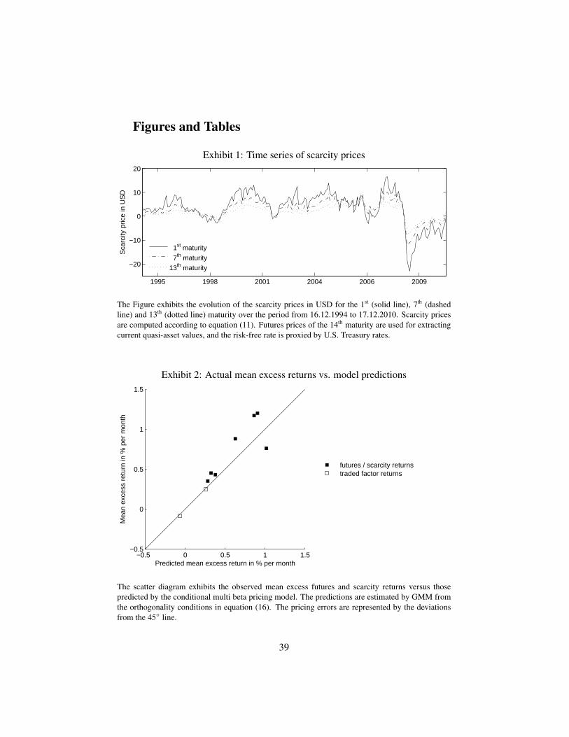
Figures and Tables

Exhibit 1: Time series of scarcity prices

1995 1998 2001 2004 2006 2009

−20

−10

0

10

20

Sca

rcity

pric

e in

US

D

1st maturity

7th maturity

13th maturity

The Figure exhibits the evolution of the scarcity prices in USD for the 1st (solid line), 7th (dashedline) and 13th (dotted line) maturity over the period from 16.12.1994 to 17.12.2010. Scarcity pricesare computed according to equation (11). Futures prices of the 14th maturity are used for extractingcurrent quasi-asset values, and the risk-free rate is proxied by U.S. Treasury rates.

Exhibit 2: Actual mean excess returns vs. model predictions

−0.5 0 0.5 1 1.5−0.5

0

0.5

1

1.5

Predicted mean excess return in % per month

Mea

n ex

cess

ret

urn

in %

per

mon

th

futures / scarcity returnstraded factor returns

The scatter diagram exhibits the observed mean excess futures and scarcity returns versus thosepredicted by the conditional multi beta pricing model. The predictions are estimated by GMM fromthe orthogonality conditions in equation (16). The pricing errors are represented by the deviationsfrom the 45 line.

39

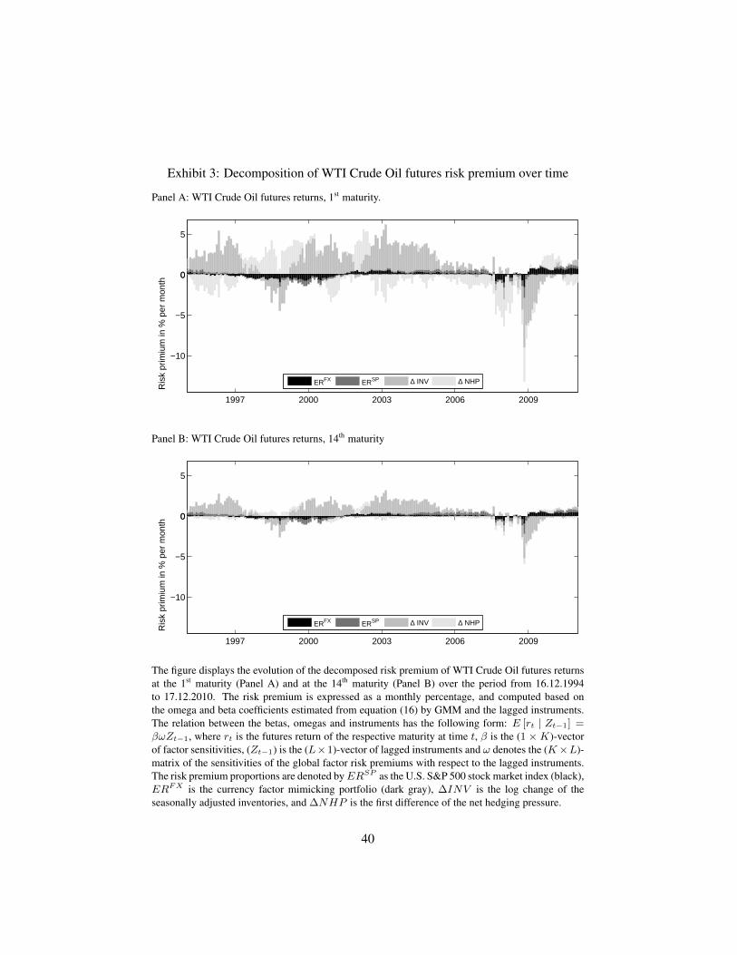
Exhibit 3: Decomposition of WTI Crude Oil futures risk premium over time

Panel A: WTI Crude Oil futures returns, 1st maturity.

1997 2000 2003 2006 20090

5

1997 2000 2003 2006 2009

−10

−5

0

Ris

k pr

imiu

m in

% p

er m

onth

ERFX ERSP ∆ INV ∆ NHP

Panel B: WTI Crude Oil futures returns, 14th maturity

1997 2000 2003 2006 20090

5

1997 2000 2003 2006 2009

−10

−5

0

Ris

k pr

imiu

m in

% p

er m

onth

ERFX ERSP ∆ INV ∆ NHP

The figure displays the evolution of the decomposed risk premium of WTI Crude Oil futures returnsat the 1st maturity (Panel A) and at the 14th maturity (Panel B) over the period from 16.12.1994to 17.12.2010. The risk premium is expressed as a monthly percentage, and computed based onthe omega and beta coefficients estimated from equation (16) by GMM and the lagged instruments.The relation between the betas, omegas and instruments has the following form: E [rt | Zt−1] =βωZt−1, where rt is the futures return of the respective maturity at time t, β is the (1 ×K)-vectorof factor sensitivities, (Zt−1) is the (L×1)-vector of lagged instruments and ω denotes the (K×L)-matrix of the sensitivities of the global factor risk premiums with respect to the lagged instruments.The risk premium proportions are denoted byERSP as the U.S. S&P 500 stock market index (black),ERFX is the currency factor mimicking portfolio (dark gray), ∆INV is the log change of theseasonally adjusted inventories, and ∆NHP is the first difference of the net hedging pressure.

40

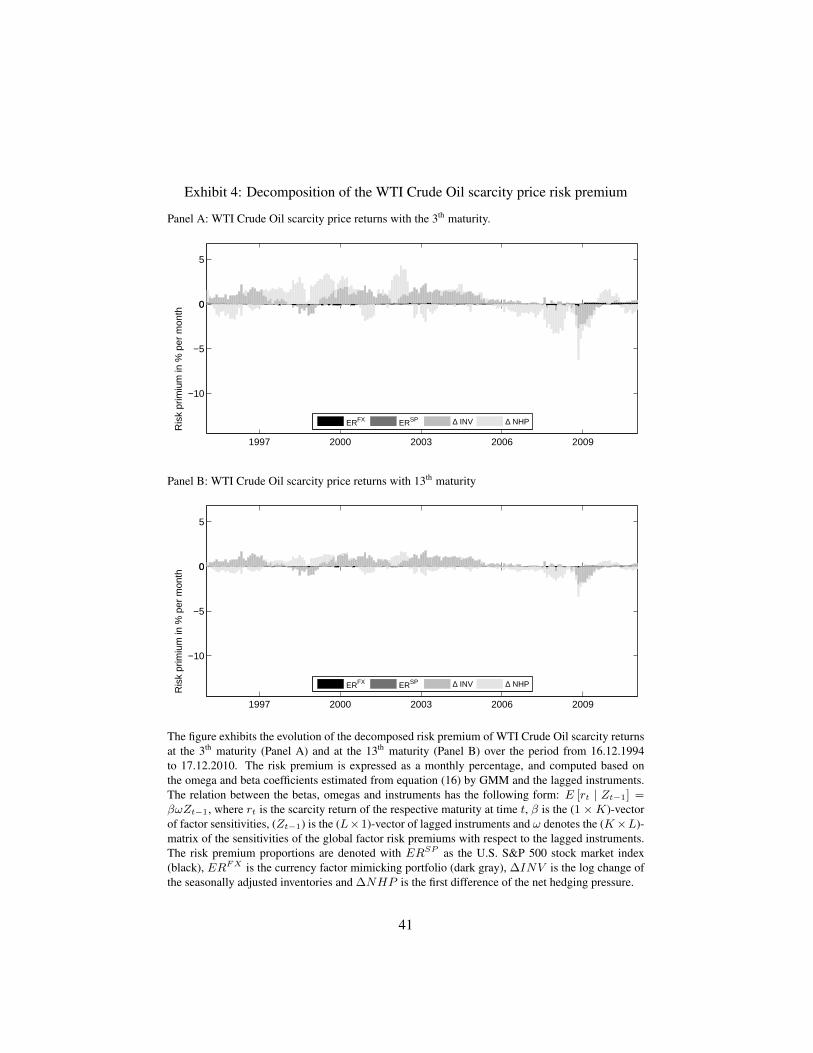
Exhibit 4: Decomposition of the WTI Crude Oil scarcity price risk premium

Panel A: WTI Crude Oil scarcity price returns with the 3th maturity.

1997 2000 2003 2006 20090

5

1997 2000 2003 2006 2009

−10

−5

0

Ris

k pr

imiu

m in

% p

er m

onth

ERFX ERSP ∆ INV ∆ NHP

Panel B: WTI Crude Oil scarcity price returns with 13th maturity

1997 2000 2003 2006 20090

5

1997 2000 2003 2006 2009

−10

−5

0

Ris

k pr

imiu

m in

% p

er m

onth

ERFX ERSP ∆ INV ∆ NHP

The figure exhibits the evolution of the decomposed risk premium of WTI Crude Oil scarcity returnsat the 3th maturity (Panel A) and at the 13th maturity (Panel B) over the period from 16.12.1994to 17.12.2010. The risk premium is expressed as a monthly percentage, and computed based onthe omega and beta coefficients estimated from equation (16) by GMM and the lagged instruments.The relation between the betas, omegas and instruments has the following form: E [rt | Zt−1] =βωZt−1, where rt is the scarcity return of the respective maturity at time t, β is the (1×K)-vectorof factor sensitivities, (Zt−1) is the (L×1)-vector of lagged instruments and ω denotes the (K×L)-matrix of the sensitivities of the global factor risk premiums with respect to the lagged instruments.The risk premium proportions are denoted with ERSP as the U.S. S&P 500 stock market index(black), ERFX is the currency factor mimicking portfolio (dark gray), ∆INV is the log change ofthe seasonally adjusted inventories and ∆NHP is the first difference of the net hedging pressure.

41

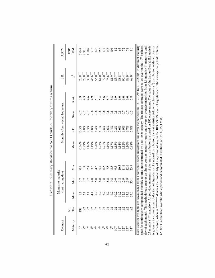
Exh

ibit

5:Su

mm

ary

stat

istic

sfo

rWT

ICru

deoi

lmon

thly

futu

res

retu

rns

Mon

ths

tom

atur

ityC

ontr

act

(las

ttra

ding

day)

Mon

thly

(fou

rwee

ks)l

ogre

turn

J.B

.A

DT

V

No.

USD

Mat

urity

Obs

.M

ean

Max

Min

Mea

nS.

D.

Skew

.K

urt.

χ2

MM

1st19

21.

11.

70.

40.

76%

10.5

%-0

.73.

920

.8**

*7’

047

2nd19

22.

12.

71.

40.

99%

9.8%

-0.7

4.3

28.8

***

2’91

03rd

192

3.1

3.7

2.4

1.16

%9.

3%-0

.74.

638

.0**

*1’

107

4th19

24.

14.

83.

51.

19%

8.8%

-0.8

4.9

46.6

***

535

5th19

25.

25.

84.

51.

20%

8.4%

-0.8

5.1

55.0

***

326

6th19

26.

26.

85.

41.

22%

8.1%

-0.8

5.4

64.0

***

253

7th19

27.

27.

86.

51.

21%

7.8%

-0.8

5.6

72.0

***

177

8th19

28.

28.

87.

51.

19%

7.6%

-0.8

5.7

78.8

***

143

9th19

29.

29.

88.

51.

17%

7.4%

-0.8

5.8

81.9

***

104

10th

192

10.2

10.9

9.5

1.15

%7.

2%-0

.85.

985

.7**

*82

11th

192

11.2

11.8

10.5

1.14

%7.

0%-0

.86.

088

.8**

*65

12th

192

12.3

12.9

11.6

1.12

%6.

9%-0

.76.

090

.4**

*72

13th

192

13.3

13.9

12.6

1.10

%6.

7%-0

.76.

089

.9**

*71

14th

192

27.0

30.1

23.9

0.88

%5.

8%-0

.35.

868

.0**

*80

Dat

aus

edfo

rthi

sta

ble

are

dow

nloa

ded

from

Tho

mso

nR

eute

rsD

atas

trea

man

dco

vert

hepe

riod

from

16.1

2.19

94to

17.1

2.20

10.1

4di

ffer

entm

atur

itysp

ecifi

cco

ntin

uous

lyco

mpo

unde

dm

onth

lyre

turn

sar

eco

nstr

ucte

dby

aro

ll-ov

erst

rate

gy.

The

futu

res

cont

ract

sw

ere

rolle

dov

eron

the

10th

busi

ness

day

ofea

chm

onth

.Thi

sm

etho

dolo

gyen

sure

san

alm

ostc

onst

antm

atur

ityre

turn

and

cove

rson

aver

age

mat

uriti

esfr

om1.

1m

onth

s(1

stm

atur

ity)u

ntil

27m

onth

s(1

4thm

atur

ity).

All

prov

ided

mom

ents

ofth

ere

turn

dist

ribu

tion

are

base

don

192

obse

rvat

ions

.The

valu

eof

the

Jarq

ue-B

era

(J.B

.)st

atis

ticis

give

nin

the

colu

mn

ten.

Und

erth

enu

llhy

poth

esis

ofa

norm

aldi

stri

butio

n,th

ete

stst

atis

tics

follo

ws

ach

i-sq

uare

(χ2)d

istr

ibut

ion

with

two

degr

ees

offr

eedo

m,w

here

as*/

**/*

**de

note

sth

epr

obab

ility

ofa

reje

ctio

nofH

0on

the

10%

/5%

/1%

leve

lof

sign

ifica

nce.

The

aver

age

daily

trad

evo

lum

e(A

DV

T)i

sca

lcul

ated

over

the

who

lepe

riod

and

deno

min

ated

inm

illio

nsof

USD

(USD

MM

).

42

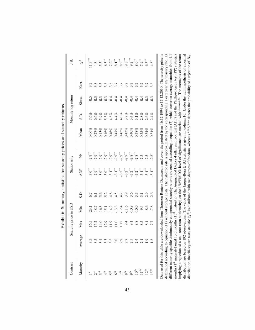
Exh

ibit

6:Su

mm

ary

stat

istic

sfo

rsca

rcity

pric

esan

dsc

arci

tyre

turn

s

Con

trac

tSc

arci

typr

ice

inU

SDSt

atio

nari

tyM

onth

lylo

gre

turn

J.B

.

Mat

urity

Ave

rage

Max

Min

S.D

.A

DF

PPM

ean

S.D

.Sk

ew.

Kur

t.χ2

1st3.

516

.5-2

3.1

6.7

-3.0

**-2

.9**

0.06

%7.

6%-0

.53.

711

.3**

*

2nd3.

515

.2-1

8.7

6.1

-2.9

**-2

.9**

0.27

%6.

6%-0

.33.

34.

33rd

3.4

14.0

-16.

35.

6-3

.0**

-2.9

**0.

43%

5.9%

-0.3

3.5

5.5*

4th3.

312

.9-1

5.1

5.2

-3.0

**-2

.9**

0.46

%5.

3%-0

.33.

66.

5**

5th3.

211

.9-1

4.2

4.8

-3.1

**-2

.9**

0.46

%4.

8%-0

.43.

67.

2**

6th3.

011

.0-1

3.3

4.5

-3.1

**-2

.9**

0.47

%4.

4%-0

.43.

78.

1**

7th2.

910

.2-1

2.4

4.2

-3.2

**-2

.9**

0.45

%4.

0%-0

.43.

78.

9**

8th2.

79.

4-1

1.6

3.9

-3.2

**-2

.9**

0.43

%3.

7%-0

.43.

79.

3***

9th2.

59.

1-1

0.8

3.6

-3.2

**-2

.8**

0.40

%3.

4%-0

.43.

79.

2***

10th

2.4

8.8

-10.

03.

3-3

.2**

-2.8

**0.

38%

3.1%

-0.4

3.7

8.0**

11th

2.1

8.5

-9.4

3.1

-3.1

**-2

.50.

35%

2.8%

-0.4

3.7

7.9**

12th

1.9

8.1

-8.6

2.9

-3.1

**-2

.50.

34%

2.6%

-0.3

3.7

6.5**

13th

1.8

7.7

-7.8

2.6

-3.1

**-2

.8*

0.31

%2.

4%-0

.33.

64.

8*

Dat

aus

edfo

rthi

sta

ble

are

dow

nloa

ded

from

Tho

mso

nR

eute

rsD

atas

trea

man

dco

vert

hepe

riod

from

16.1

2.19

94to

17.1

2.20

10.T

hesc

arci

typr

ice

isde

term

ined

acco

rdin

gto

equa

tion

(11)

with

outs

tora

geco

sts.

The

risk

-fre

era

teis

appr

oxim

ated

byth

eco

rres

pond

ing

1or

2ye

arU

Str

easu

ryra

te.

13di

ffer

entm

atur

itysp

ecifi

cco

ntin

uous

lyco

mpo

unde

dsc

arci

tyre

turn

sar

ecr

eate

dac

cord

ing

toeq

uatio

n(7

),w

hich

cove

ron

aver

age

mat

uriti

esfr

om1.

1m

onth

s(1

stm

atur

ity)u

ntil

13.3

mon

ths

(13th

mat

urity

).T

heA

ugm

ente

dD

icke

y-Fu

lleru

nitr

oott

est(

AD

F)an

dth

ePh

illip

s-Pe

rron

test

(PP)

stat

istic

sim

plyi

nga

reje

ctio

nof

aun

itro

ot(n

on-s

tatio

nari

ty)

onth

e1%

/5%

/10%

leve

lof

sign

ifica

nce

are

mar

ked

with

***/

**/*

.T

hem

omen

tsof

the

retu

rndi

stri

butio

nar

eba

sed

on19

2ob

serv

atio

ns.

The

valu

eof

the

Jarq

ue-B

era

(J.B

.)st

atis

ticis

give

nin

colu

mn

10.

Und

erth

enu

llhy

poth

esis

ofa

norm

aldi

stri

butio

n,th

ech

i-sq

uare

test

sst

atis

tic(χ

2)i

sdi

stri

bute

dw

ithtw

ode

gree

sof

free

dom

,whe

reas

*/**

/***

deno

tes

the

prob

abili

tyof

are

ject

ion

ofH

0.

43

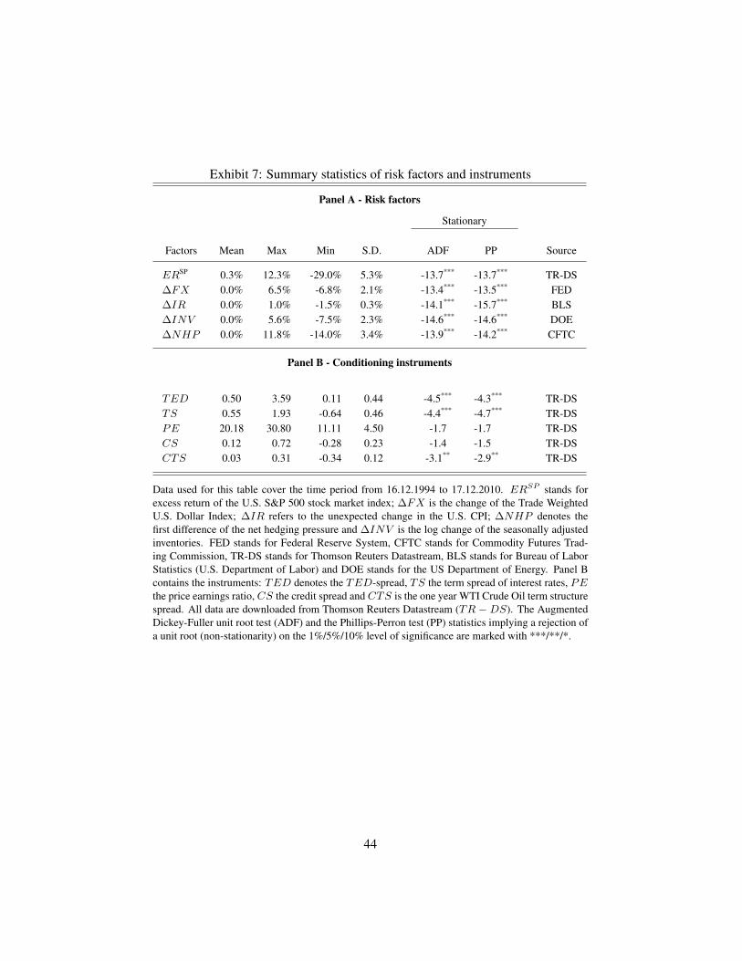
Exhibit 7: Summary statistics of risk factors and instruments

Panel A - Risk factors

Stationary

Factors Mean Max Min S.D. ADF PP Source

ERSP 0.3% 12.3% -29.0% 5.3% -13.7*** -13.7*** TR-DS∆FX 0.0% 6.5% -6.8% 2.1% -13.4*** -13.5*** FED∆IR 0.0% 1.0% -1.5% 0.3% -14.1*** -15.7*** BLS∆INV 0.0% 5.6% -7.5% 2.3% -14.6*** -14.6*** DOE∆NHP 0.0% 11.8% -14.0% 3.4% -13.9*** -14.2*** CFTC

Panel B - Conditioning instruments

TED 0.50 3.59 0.11 0.44 -4.5*** -4.3*** TR-DSTS 0.55 1.93 -0.64 0.46 -4.4*** -4.7*** TR-DSPE 20.18 30.80 11.11 4.50 -1.7 -1.7 TR-DSCS 0.12 0.72 -0.28 0.23 -1.4 -1.5 TR-DSCTS 0.03 0.31 -0.34 0.12 -3.1** -2.9** TR-DS

Data used for this table cover the time period from 16.12.1994 to 17.12.2010. ERSP stands forexcess return of the U.S. S&P 500 stock market index; ∆FX is the change of the Trade WeightedU.S. Dollar Index; ∆IR refers to the unexpected change in the U.S. CPI; ∆NHP denotes thefirst difference of the net hedging pressure and ∆INV is the log change of the seasonally adjustedinventories. FED stands for Federal Reserve System, CFTC stands for Commodity Futures Trad-ing Commission, TR-DS stands for Thomson Reuters Datastream, BLS stands for Bureau of LaborStatistics (U.S. Department of Labor) and DOE stands for the US Department of Energy. Panel Bcontains the instruments: TED denotes the TED-spread, TS the term spread of interest rates, PEthe price earnings ratio, CS the credit spread and CTS is the one year WTI Crude Oil term structurespread. All data are downloaded from Thomson Reuters Datastream (TR −DS). The AugmentedDickey-Fuller unit root test (ADF) and the Phillips-Perron test (PP) statistics implying a rejection ofa unit root (non-stationarity) on the 1%/5%/10% level of significance are marked with ***/**/*.

44

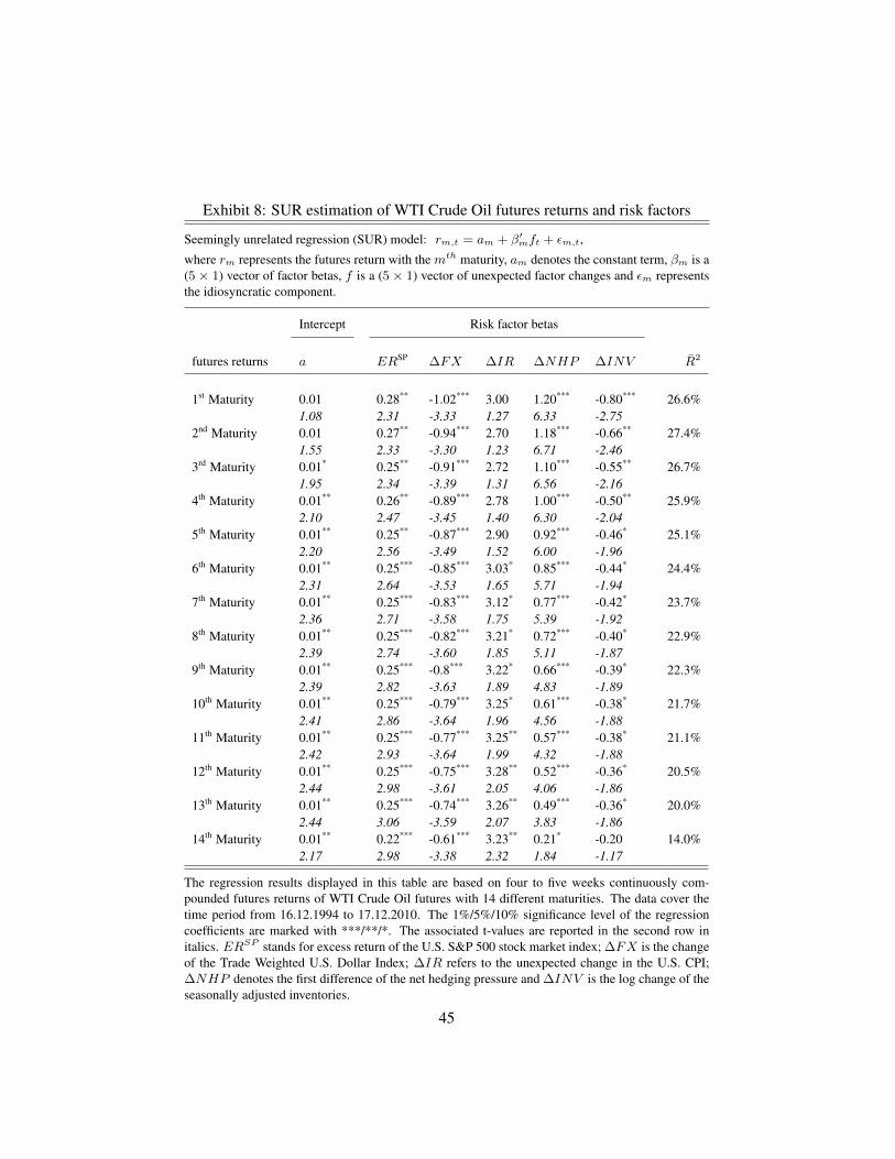
Exhibit 8: SUR estimation of WTI Crude Oil futures returns and risk factors

Seemingly unrelated regression (SUR) model: rm,t = am + β′mft + εm,t,

where rm represents the futures return with the mth maturity, am denotes the constant term, βm is a(5 × 1) vector of factor betas, f is a (5 × 1) vector of unexpected factor changes and εm representsthe idiosyncratic component.

Intercept Risk factor betas

futures returns a ERSP ∆FX ∆IR ∆NHP ∆INV R2

1st Maturity 0.01 0.28** -1.02*** 3.00 1.20*** -0.80*** 26.6%1.08 2.31 -3.33 1.27 6.33 -2.75

2nd Maturity 0.01 0.27** -0.94*** 2.70 1.18*** -0.66** 27.4%1.55 2.33 -3.30 1.23 6.71 -2.46

3rd Maturity 0.01* 0.25** -0.91*** 2.72 1.10*** -0.55** 26.7%1.95 2.34 -3.39 1.31 6.56 -2.16

4th Maturity 0.01** 0.26** -0.89*** 2.78 1.00*** -0.50** 25.9%2.10 2.47 -3.45 1.40 6.30 -2.04

5th Maturity 0.01** 0.25** -0.87*** 2.90 0.92*** -0.46* 25.1%2.20 2.56 -3.49 1.52 6.00 -1.96

6th Maturity 0.01** 0.25*** -0.85*** 3.03* 0.85*** -0.44* 24.4%2.31 2.64 -3.53 1.65 5.71 -1.94

7th Maturity 0.01** 0.25*** -0.83*** 3.12* 0.77*** -0.42* 23.7%2.36 2.71 -3.58 1.75 5.39 -1.92

8th Maturity 0.01** 0.25*** -0.82*** 3.21* 0.72*** -0.40* 22.9%2.39 2.74 -3.60 1.85 5.11 -1.87

9th Maturity 0.01** 0.25*** -0.8*** 3.22* 0.66*** -0.39* 22.3%2.39 2.82 -3.63 1.89 4.83 -1.89

10th Maturity 0.01** 0.25*** -0.79*** 3.25* 0.61*** -0.38* 21.7%2.41 2.86 -3.64 1.96 4.56 -1.88

11th Maturity 0.01** 0.25*** -0.77*** 3.25** 0.57*** -0.38* 21.1%2.42 2.93 -3.64 1.99 4.32 -1.88

12th Maturity 0.01** 0.25*** -0.75*** 3.28** 0.52*** -0.36* 20.5%2.44 2.98 -3.61 2.05 4.06 -1.86

13th Maturity 0.01** 0.25*** -0.74*** 3.26** 0.49*** -0.36* 20.0%2.44 3.06 -3.59 2.07 3.83 -1.86

14th Maturity 0.01** 0.22*** -0.61*** 3.23** 0.21* -0.20 14.0%2.17 2.98 -3.38 2.32 1.84 -1.17

The regression results displayed in this table are based on four to five weeks continuously com-pounded futures returns of WTI Crude Oil futures with 14 different maturities. The data cover thetime period from 16.12.1994 to 17.12.2010. The 1%/5%/10% significance level of the regressioncoefficients are marked with ***/**/*. The associated t-values are reported in the second row initalics. ERSP stands for excess return of the U.S. S&P 500 stock market index; ∆FX is the changeof the Trade Weighted U.S. Dollar Index; ∆IR refers to the unexpected change in the U.S. CPI;∆NHP denotes the first difference of the net hedging pressure and ∆INV is the log change of theseasonally adjusted inventories.

45

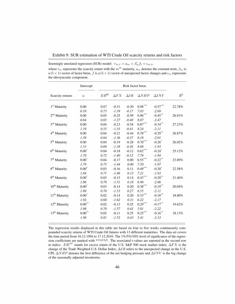
Exhibit 9: SUR estimation of WTI Crude Oil scarcity returns and risk factors

Seemingly unrelated regression (SUR) model: rm,t = am + β′mft + εm,t,

where rm represents the scarcity return with the mth maturity, am denotes the constant term, βm isa (5× 1) vector of factor betas, f is a (5× 1) vector of unexpected factor changes and εm representsthe idiosyncratic component.

Intercept Risk factor betas

Scarcity returns a ERSP ∆FX ∆IR ∆NHP ∆INV R2

1st Maturity 0.00 0.07 -0.31 -0.30 0.98*** -0.57*** 22.78%0.10 0.73 -1.39 -0.17 7.03 -2.69

2nd Maturity 0.00 0.05 -0.25 -0.59 0.96*** -0.45** 26.91%0.64 0.65 -1.27 -0.40 8.07 -2.47

3rd Maturity 0.00 0.04 -0.23 -0.54 0.87*** -0.34** 27.23%1.19 0.55 -1.33 -0.41 8.24 -2.11

4th Maturity 0.00 0.04 -0.21 -0.44 0.78*** -0.29** 26.87%1.39 0.64 -1.36 -0.37 8.18 -2.01

5th Maturity 0.00 0.04 -0.19 -0.28 0.70*** -0.26* 26.02%1.53 0.69 -1.38 -0.26 8.00 -1.93

6th Maturity 0.00* 0.04 -0.18 -0.12 0.62*** -0.24* 25.12%1.70 0.72 -1.40 -0.12 7.79 -1.94

7th Maturity 0.00* 0.04 -0.17 0.00 0.55*** -0.22** 23.89%1.79 0.75 -1.44 0.00 7.50 -1.97

8th Maturity 0.00* 0.03 -0.16 0.11 0.49*** -0.20* 22.58%1.84 0.71 -1.46 0.13 7.21 -1.93

9th Maturity 0.00* 0.03 -0.15 0.14 0.43*** -0.20** 21.46%1.86 0.78 -1.51 0.18 6.90 -2.06

10th Maturity 0.00* 0.03 -0.14 0.20 0.38*** -0.19** 20.04%1.89 0.78 -1.53 0.27 6.55 -2.11

11th Maturity 0.00* 0.02 -0.14 0.20 0.33*** -0.18** 18.80%1.92 0.68 -1.62 0.31 6.22 -2.17

12th Maturity 0.00** 0.02 -0.13 0.25 0.29*** -0.17** 19.62%1.98 0.70 -1.57 0.41 5.81 -2.22

13th Maturity 0.00** 0.02 -0.11 0.25 0.25*** -0.16** 18.13%1.98 0.81 -1.52 0.43 5.41 -2.33

The regression results displayed in this table are based on four to five weeks continuously com-pounded scarcity returns of WTI Crude Oil futures with 13 different maturities. The data set coversthe time period from 16.12.1994 to 17.12.2010. The 1%/5%/10% level of significance of the regres-sion coefficients are marked with ***/**/*. The associated t-values are reported in the second rowin italics. ERSP stands for excess return of the U.S. S&P 500 stock market index; ∆FX is thechange of the Trade Weighted U.S. Dollar Index; ∆IR refers to the unexpected change in the U.S.CPI; ∆NHP denotes the first difference of the net hedging pressure and ∆INV is the log changeof the seasonally adjusted inventories.

46

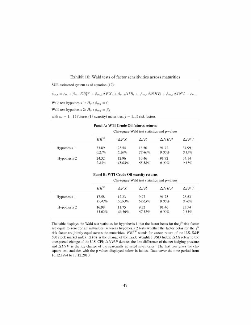
Exhibit 10: Wald tests of factor sensitivities across maturities

SUR estimated system as of equation (12):

rm,t = cm + βm,1ERSPt + βm,2∆FXt + βm,3∆IRt + βm,4∆NHPt + βm,5∆INVt + εm,t

Wald test hypothesis 1: H0 : βmj = 0

Wald test hypothesis 2: H0 : βmj = βj

with m = 1...14 futures (13 scarcity) maturities, j = 1...5 risk factors

Panel A: WTI Crude Oil futures returnsChi-square Wald test statistics and p-values

ERSP ∆FX ∆IR ∆NHP ∆INV

Hypothesis 1 33.89 23.54 16.50 91.72 34.990.21% 5.20% 28.40% 0.00% 0.15%

Hypothesis 2 24.32 12.96 10.46 91.72 34.142.83% 45.08% 65.58% 0.00% 0.11%

Panel B: WTI Crude Oil scarcity returnsChi-square Wald test statistics and p-values

ERSP ∆FX ∆IR ∆NHP ∆INV

Hypothesis 1 17.58 12.23 9.97 91.75 28.5317.43% 50.93% 69.63% 0.00% 0.76%

Hypothesis 2 16.98 11.75 9.32 91.46 23.5415.02% 46.56% 67.52% 0.00% 2.35%

The table displays the Wald test statistics for hypothesis 1 that the factor betas for the jth risk factorare equal to zero for all maturities, whereas hypothesis 2 tests whether the factor betas for the jth

risk factor are jointly equal across the maturities. ERSP stands for excess return of the U.S. S&P500 stock market index; ∆FX is the change of the Trade Weighted USD Index; ∆IR refers to theunexpected change of the U.S. CPI; ∆NHP denotes the first difference of the net hedging pressureand ∆INV is the log change of the seasonally adjusted inventories. The first row gives the chi-square test statistics with the p-values displayed below in italics. Data cover the time period from16.12.1994 to 17.12.2010.

47

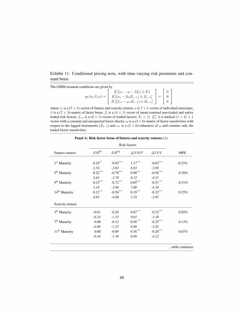
Exhibit 11: Conditional pricing tests, with time-varying risk premiums and con-stant betas

The GMM moment conditions are given by

gT (a, β, ω) =

E [(rt − a− βft)⊗ Ft]E [(rt − βωZt−1)⊗ Zt−1]

E [(fτt − ωτZt−1)⊗ Zt−1]

=

0

0

0

where rt is a (7× 1)-vector of futures and scarcity returns; a is 7× 1-vector of individual intercepts;β is a (7 × 3)-matrix of factor betas; ft is a (4 × 1) vector of mean centered non-traded and nativetraded risk factors; fτ,t is a (2 × 1)-vector of traded factors; Ft = [1 f ′t ]

′ is a stacked (1 + 4) × 1vector with a constant and unexpected factor shocks; ω is a (3× 6)-matrix of factor sensitivities withrespect to the lagged instruments (Zt−1) and ωτ is a (2 × 6)-submatrix of ω and contains only thetraded factor sensitivities.

Panel A: Risk factor betas of futures and scarcity returns (β)

Risk factors

Futures returns ERSP ERFX ∆NHP ∆INV MPE

1st Maturity 0.24** -0.95*** 1.17*** -0.65*** -0.25%2.54 -3.63 8.83 -3.98

5th Maturity 0.22*** -0.79*** 0.90*** -0.56*** 0.30%2.63 -3.78 8.12 -4.21

9th Maturity 0.23*** -0.72*** 0.65*** -0.51*** 0.31%3.14 -3.99 7.00 -4.34

14th Maturity 0.23*** -0.56*** 0.19*** -0.32*** 0.25%4.65 -4.00 3.18 -3.91

Scarcity returns

3th Maturity -0.01 -0.20 0.87*** -0.32*** 0.05%-0.24 -1.33 9.65 -3.38

7th Maturity 0.00 -0.12 0.56*** -0.25*** 0.13%-0.09 -1.25 8.90 -3.82

11th Maturity 0.00 -0.09 0.36*** -0.20*** 0.07%-0.16 -1.39 8.09 -4.22

...table continues

48

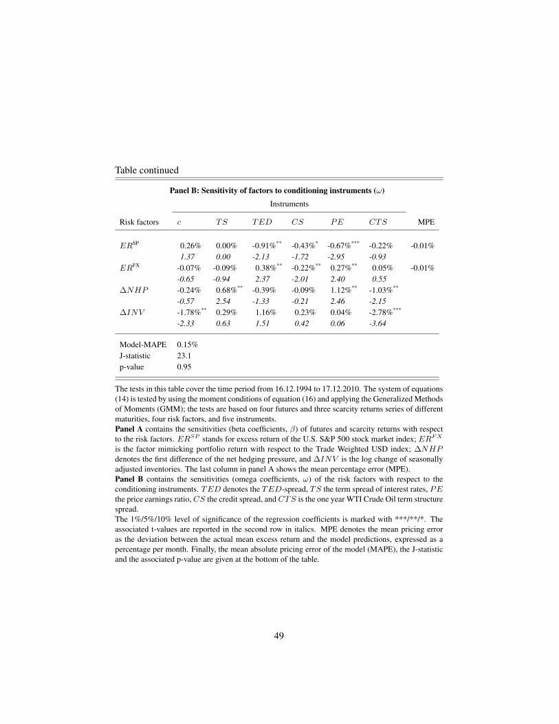
Table continued

Panel B: Sensitivity of factors to conditioning instruments (ω)

Instruments

Risk factors c TS TED CS PE CTS MPE

ERSP 0.26% 0.00% -0.91%** -0.43%* -0.67%*** -0.22% -0.01%1.37 0.00 -2.13 -1.72 -2.95 -0.93

ERFX -0.07% -0.09% 0.38%** -0.22%** 0.27%** 0.05% -0.01%-0.65 -0.94 2.37 -2.01 2.40 0.55

∆NHP -0.24% 0.68%** -0.39% -0.09% 1.12%** -1.03%**

-0.57 2.54 -1.33 -0.21 2.46 -2.15∆INV -1.78%** 0.29% 1.16% 0.23% 0.04% -2.78%***

-2.33 0.63 1.51 0.42 0.06 -3.64

Model-MAPE 0.15%J-statistic 23.1p-value 0.95

The tests in this table cover the time period from 16.12.1994 to 17.12.2010. The system of equations(14) is tested by using the moment conditions of equation (16) and applying the Generalized Methodsof Moments (GMM); the tests are based on four futures and three scarcity returns series of differentmaturities, four risk factors, and five instruments.Panel A contains the sensitivities (beta coefficients, β) of futures and scarcity returns with respectto the risk factors. ERSP stands for excess return of the U.S. S&P 500 stock market index; ERFX

is the factor mimicking portfolio return with respect to the Trade Weighted USD index; ∆NHPdenotes the first difference of the net hedging pressure, and ∆INV is the log change of seasonallyadjusted inventories. The last column in panel A shows the mean percentage error (MPE).Panel B contains the sensitivities (omega coefficients, ω) of the risk factors with respect to theconditioning instruments. TED denotes the TED-spread, TS the term spread of interest rates, PEthe price earnings ratio,CS the credit spread, andCTS is the one year WTI Crude Oil term structurespread.The 1%/5%/10% level of significance of the regression coefficients is marked with ***/**/*. Theassociated t-values are reported in the second row in italics. MPE denotes the mean pricing erroras the deviation between the actual mean excess return and the model predictions, expressed as apercentage per month. Finally, the mean absolute pricing error of the model (MAPE), the J-statisticand the associated p-value are given at the bottom of the table.

49