Embed Size (px)
Citation preview
HAL Id: hal-00936578https://hal.archives-ouvertes.fr/hal-00936578
Submitted on 8 Sep 2020
HAL is a multi-disciplinary open accessarchive for the deposit and dissemination of sci-entific research documents, whether they are pub-lished or not. The documents may come fromteaching and research institutions in France orabroad, or from public or private research centers.
L’archive ouverte pluridisciplinaire HAL, estdestinée au dépôt et à la diffusion de documentsscientifiques de niveau recherche, publiés ou non,émanant des établissements d’enseignement et derecherche français ou étrangers, des laboratoirespublics ou privés.
Distributed under a Creative Commons Attribution| 4.0 International License
Scaling study of cavitation pitting from cavitating jetsand ultrasonic horns
Arvind Jayaprakash, Jin-Keun Choi, Georges Chahine, Farrel Martin, MartinDonnelly, Jean-Pierre Franc, Ayat Karimi
To cite this version:Arvind Jayaprakash, Jin-Keun Choi, Georges Chahine, Farrel Martin, Martin Donnelly, et al.. Scalingstudy of cavitation pitting from cavitating jets and ultrasonic horns. Wear, Elsevier, 2012, 296 (1-2),pp.619-629. �10.1016/j.wear.2012.07.025�. �hal-00936578�
Wear, 2012 (in press)
1
Scaling Study of Cavitation Pitting from Cavitating Jets
and Ultrasonic Horns
Arvind Jayaprakash1, Jin-Keun Choi
1, Georges L. Chahine
1,
Farrel Martin2, Martin Donnelly
3, Jean-Pierre FRANC
4, and Ayat Karimi
5
Abstract
Cavitation erosion prediction and characterization of cavitation field strength are of interest to
industries suffering from cavitation erosion detrimental effects. One means to evaluate cavitation fields and
materials is to examine pitting rates during the incubation period, where the test sample undergoes localized
permanent deformations shaped as individual pits. In this study, samples from three metallic materials, an
Aluminum alloy (Al7075), a Nickel Aluminum Bronze (NAB) and a Duplex Stainless Steel (SS A2205) were
subjected to a vast range of cavitation intensities generated by cavitating jets at different driving pressures and
by an ultrasonic horn. The resulting pitted sample surfaces were examined and characterized with a non-
contact 3D optical scanner and the resulting damage computer-analyzed. A statistical analysis of the pit
population and its characteristics was then carried out. It was found that the various cavitation field strengths
can be correlated to the measured pit distributions and that two characteristic quantities: a characteristic
number of pits per unit surface area and unit time, and a characteristic pit diameter or a characteristic pit
depth can be attributed to a given “cavitation intensity level”. This characterization concept can be used in the
future to study the cavitation intensity of the full scale and to develop methods of full scale predictions based
on model scale erosion data.
Keywords: Cavitation erosion; Erosion testing; Steel; Non-ferrous metals; Erosion modeling
1 DYNAFLOW, INC., Jessup, Maryland, U.S.A. email: [email protected]
2 Naval Research Laboratory, email: [email protected]
3 Naval Surface Warfare Center Carderock Division, [email protected]
4 Grenoble University (LEGI) Grenoble, France, email: [email protected]
5 EPFL, Lausanne, Switzerland, email: [email protected]
Wear, 2012 (in press)
2
1 Introduction
Evaluation of a new material’s resistance to cavitation erosion often relies on comparative
laboratory studies involving accelerated erosion
tests. This is the case because scaled erosion tests
are either not possible, too slow, or because
cavitation erosion scaling is still not fully
understood scientifically. Accelerated erosion tests
to evaluate a material or select one material
among several, by definition, involves subjecting
material samples to a cavitation field that produces
measurable erosion over a short period of time.
This, almost by definition, involves a different type
of cavitation erosion than what is present in the
actual cavitation field the tested material is
destined to be subjected to. Casually, the
laboratory determined ranking of the materials in
the accelerated erosion tests is practically assumed
to hold in the real application field. However,
evidence exists that this may not always be the
case, since some materials at least react differently
to cavitation fields of different strength [1-4].
Fundamentally, the mechanical process of
cavitation erosion results from successive
individual and collective cavity collapses, which
generate local high amplitude, short duration
loads. The overall picture is that bubble nuclei in
the liquid grow explosively in low pressure regions
forming cavitation bubble clouds [5-9]. These
subsequently collapse generating very high local
pressures and temperatures [10-11]. In addition,
when the bubbles collapse very close or at the
material surface, micro reentrant jets from bubble
large deformations vector towards the material
and impact its surface [12-15]. When the pressure
loads exceed the elastic limit of the material, the
material undergoes permanent deformations
leaving microscopic pits [16]. This initial incubation
period of the material response to the erosion
cavitation flow field does not involve any mass
loss. With repeated impacts, hardening of the
material surface layer develops, the deformation
of the material accumulates, and finally micro-
failures occur resulting in material removal and
thus weight loss.
One method to investigate a portion of
the above dynamics is to conduct pitting tests, i.e.
short duration tests during the incubation period,
where isolated (not overlapping) pits can be
identified and characterized [1]. By doing so, the
material is used as a recorder of the highest
pressures in the cavitating field, since each
material acts as a high pass filter and records as
pits only the cavitating field pressure peaks at the
material surface that exceed its yield stress and
plastically deform permanently. Observation of
pits for the purpose of evaluating the cavitation
field intensity dates back to the early 1900’s when Parsons and Cook [17] observed the depth and
dimensions of the pitted areas, and researchers
reported the pitting location relative to the
cavitation cloud shape and statistics such as the
number and the depth of pitting [18-20]. Knapp
[19-21] introduced the idea that the pits could be
used to understand the intensity of the cavitation
field. Similar ideas of observing pits to represent
the cavitation field was used in hydraulic turbine
cavitation erosion studies [22], where it was found
that the cavitation aggressiveness in the full scale
is more severe than that of the model scale.
Recent studies using pitting tests includes the use
of thin copper foil in order to capture relative small
magnitude impacts [23], analysis of pitting to
determine the impact loads for a modeling effort
for ductile metals [24], evaluation of flow
aggressiveness in the study of hydraulic turbine
flows [25], and applications to the erosion studies
of marine propellers [26,27]. With the advance of
modern imaging and micro-measurement
technologies, recent studies reveal more details of
the pit shapes and statistics [28,29]. However,
these studies did not provide a unified description
of the cavitation field based on the pitting tests.
In this paper, we model the pit statistics as
an attempt to identify parameters that
characterize the aggressiveness of a cavitation
field. Three different materials, an Aluminum alloy,
a Nickel Aluminum Bronze, and a Duplex Stainless
Steel were subjected to vastly different intensities
of cavitation field generated by acoustic horn [30]
and by DYNAJETS® cavitating jets [4,31,32] at
different driving pressures. These were provided
by the Naval Surface Warfare Center, Carderock
Division. The pit population and sizes resulting
from the tests in these different cavitation fields
were analyzed and statistically processed. Based
on this analysis, we propose a model that describes
the pitting statistics with a small number of
parameters, which in the future can be used to
define the cavitation field intensity level. The
above three materials are the same three materials
used in Franc et al. [33], and results in this paper
can be used as a comparative study with [33] of
various cavitation erosion generation methods.
The study described in this paper is an effort to
deduce a relationship between the cavitation field
intensity and the pitting statistics. This is a part of
an on-going rather large effort, in which we are
investigating experimentally and modeling
numerically the erosion process in order to relate

Wear, 2012 (in press)
3
the material erosion to the cavitation field
intensity in a predictive manner.
2 Experimental Setup and Procedure
In order to study cavitation erosion in a
controlled environment and in an accelerated
manner, several laboratory techniques to generate
cavitation have been used in the past. These
techniques include the utilization of ultrasonic
vibration to generate the cavitation, cavitation
flow loops with strong separating flows, rotating
disks, venturi cavitating flows, vortex generators,
and submerged cavitating jets. Some of these
techniques were standardized and resulted in
American Society for Testing and Materials (ASTM)
Standards [30] such as G-32 “Test Method for
Cavitation Erosion Using Vibratory Apparatus” and G-134 “Test Method for Erosion of Solid Materials
by a Cavitating Liquid Jet”. In this study, the ultrasonic test method following G32 and
cavitating jet tests were conducted at DYNAFLOW to
investigate the incubation period. The time
evolution of the weight loss of the three
considered materials was documented in [32].
2.1 Ultrasonic Cavitation Erosion Testing
We followed in our test the prescribed
ultrasonic cavitation tests ASTM G-32 method [30].
The cavitation is generated by a vibratory device
employing a magnetostrictive ultrasonic horn. The
acoustic horn was operated at 20 kHz with a peak-
to-peak amplitude of 50 μm. The amplitude was set using a bifilar microscope and maintained at
that value throughout testing. The samples were
held in place with fixed sample holders inside a
2,000 ml beaker filled with distilled water and with
the horn tip submerged 12 mm beneath the free
surface. The beakers were immersed in a water
bath maintained at 25 ±2 ºC. In the “alternative” G-
32 test configuration (also known as a stationary
specimen method), the horn tip is placed at a small
distance from the stationary material sample, here
at 0.5 mm below the tip of the horn, and the
cavitation cloud was generated in between the
two. We used 25.4 mm x 25.4 mm square samples
of the material to be tested.
The temperature, liquid beaker volume,
horn tip submergence beneath the free surface,
frequency, and amplitude of the oscillations are all
prescribed by the ASTM G-32 method. In the direct
G32 method the cavitation cloud collapses in a
hemispherical way toward the material, while in
the modified method, the cavitation bubble cloud
collapses in a cylindrical way. It is well known from
previous studies [34] that the cloud cavitation
collapsing cylindrically is much less erosive than
the hemispherically collapsing cavitation clouds,
thus the alternative methods produce less erosive
results than the direct method.
Usually, for mass loss tests, the procedure
is to expose the sample to cavitation for a given
period of time, stop the test, remove the sample,
and record weight to enable measurement of
weight loss as a function of time. The sample is
then returned for additional testing. In the pitting
tests, only one interval of above mass loss test was
conducted. The samples were polished up to a
mirror like surface so that the surface scan
conducted later will have less noise from the
existing roughness of the surface. The facility at
Naval Research Laboratory (NRL) was used to
polish the samples. The specimens were prepared
using SiC metallographic papers, starting with 240
grit and increasing fineness of 400, 600, 1200 and
1500, followed by diamond slurry polishes of
decreasing grit diameter of 10, 3, 1 and .01
microns. The final step in polishing was performed
on a vibratory polisher for a period of 12 hours.
The polished samples were kept individually in a
container, and the surface was not touched by any
other objects until the beginning of the test. As
soon as the test is completed, the sample was
dried completely by air blower and then stored
individually in a container. The tested surface was
not touched until it was examined by the optical
scanner.
2.2 DYNAJETS® Cavitating Jet Tests
The cavitating jet erosion tests used
DYNAJETS® cavitating jet nozzles, a sample holder, a
water tank, and a pump. The sample holder
ensures that the sample is held in place during the
pitting tests (Figure 1). The pitting test procedure
using this jet cavitation was as follows:
(a) The sample surface was polished up to mirror
like surface.
(b) The sample was exposed to the cavitating jet
for a predetermined period of time.
(c) The sample was taken out from its holder, and
carefully dried.
(d) The surface was scanned using an optical
profilometer.
The sample preparation and post-test procedures
was the same to that of the ultrasonic tests as
described in the preceding section.

Wear, 2012 (in press)
4
Figure 1. Nozzle and sample holder in DYNAFLOW’s “7 ksi - 5 gpm” cavitation jet erosion test loop.
3 Materials Tested
Three materials were selected for tests
under this program: Aluminum alloy 7075 – T651,
Nickel Aluminum Bronze Alloy (NAB), and Duplex
Stainless Steel SS A2205. The main properties of
the tested materials are shown in Table 1.
We also conducted Split Hopkinson
Pressure Bar (SHPB) tests on these materials to
measure the high strain rate properties of these
materials. Figure 2 compares the engineering
stress vs. engineering strain curves for Aluminum
alloy 7075 at different strain rates (1200/s ~
1825/s) and a literature data for a near zero strain
rate [35]. The SHPB curves show some oscillations,
which are typical especially near the end of curves.
This portion of data were obtained when the
sample was about to detach from the bar.
Material
Aluminum Alloy
7075 T651 (Al)
Nickel Aluminum
Bronze (NAB)
Duplex Stainless
Steel 2205 (SS)
Tensile Yield
Strength 503 MPa 355 MPa 510 MPa
Ultimate Tensile
Strength 572 MPa 683 MPa 750 MPa
Modulus of Elasticity
71.7 GPa 115 GPa 200 GPa
Elongation at Break
11% 10 ~ 18% 35%
Table 1. Tested materials and main properties.
The Aluminum alloy 7075 showed slightly
larger strain at high strain rates than the strain at
the corresponding static loading. Near zero strain,
the average slope of these curves are obtained and
compared with the literature values of the static
modulus of elasticity in Table 2. The moduli of
elasticity deduced from the slope of the stress-
strain curves from the SHPB were comparable to
the static values from the literature and from
nano-indentor measurements conducted at EPFL
[36,37].
Figure 2. Comparison of stress-strain curves of Al
7075 obtained from Split Hopkinson Pressure Bar
(SHPB) tests and a reported curve for a near zero
strain rate from literature [35].
Source
Aluminum Alloy
7075 T651
Nickel Aluminum
Bronze Alloy (NAB)
Duplex Stainless
Steel 2205 (SS)
Literature [37]
71.7 GPa 120 GPa 200 GPa
DYNAFLOW SHPB tests
67.6 GPa 127 GPa 190 GPa
Nano-indentor
tests (EPFL)
[36]
86.0 GPa 150 GPa 215 GPa
Table 2: Comparison of the modulus of elasticity
for the three materials tested.
4 Pit Analysis Techniques
4.1 Procedures
The 25.4 mm x 25.4 mm x 6.35mm mirror-
polished material samples were subjected to

Wear, 2012 (in press)
5
cavitation fields of different intensities for
predetermined time durations. The central jet
impact area where maximum pitting occurred was
chosen for detailed analysis. Optical scanning
profilometry provided by the Naval Research
Laboratory was used to measure very carefully the
surface of the pitted sample. The optical scans
were conducted over an area of 1 mm x 1 mm.
The used optical scanner Alicona InfiniteFocus G4
with 100x optical objective lens, was capable of
producing very high resolution data [38]. The
interrogation mesh size was selected to be
1.5 µm x 1.5 µm. Figure 3 shows a contour plot of
the surface data obtained from such an optical
scan of the pitted surface.
Despite the fact that the surface was
highly polished, surface level fluctuations can be
seen in the surface as a result of polishing and
machining marks, and could interfere with
automatic measurement if not filtered. This
required us to impose a threshold as a cut-off
depth, dth, that was applied during post-process of
the measured data; i.e. all elevations higher than -
dth , measured from the averaged zero level, were
ignored or cut-off. One has however to realize that
this threshold affects the statistical results as
discussed later. In addition to the above, a few
very deep pits noticed in the optical scan (as in
Figure 4) were attributed to known artifacts caused
by the optical measurement technique, and these
erroneous data were filtered out.
4.2 Pit Counting
The surface scanning profilometer
generates a full 3D discretized description of the
eroded material surface, ( , )z x y . From this
discretized mathematical description, we derived
using various geometry or particle analysis
software statistical analyses of various quantities
of interest here: number of pits, areas, volumes,
equivalent diameter, average depth, shape factor,
etc. of the pits. Because of the selection of
advancing stages of very early pitting, very little
pitting overlap occurred and individual pits could
be easily identified, and the geometric
characteristics of each individual pit could be
accurately measured and used in the statistical
analysis.
Figure 3. Typical data obtained from optical
scanning of a pitted sample. Shown here is the
actual 1.587 mm x 1.719 mm scan of Al 7075
sample pitted under a 1,100 psi DYNAJETS®
for a
duration of 2 min.
Figure 4. Typical surface levels in a vertical cut
plane obtained from optical scan of pitted
samples. This profile is obtained from the surface
shown in Figure 3.
Data Name
Computed Data Unit
Pitting Rate
N number of pits
exposure time× analyzed surface
Pits/mm
2/
s
Deformation Depth Rate
h volume of pits
exposure time× analyzed surface
µm/h
Table 3: Measured and computed data.
4.3 Cumulative Pitting Rate versus Pit Diameter
From the scanned profilometer
measurements, an average pitting rate can be
defined as the cumulative number of pits after a
given exposure time, texp, divided by texp . The
Wear, 2012 (in press)
6
actual instantaneous rate is harder to measure and
would require many time measurement points.
The deformation depth rate is also defined
similarly from the measured average pit depth,
defined as the ratio of pit volume to pit area
(Table 3).
The counted pits can be classified
according to their diameter. The cumulative
diameter distribution function of the pitting rate
can be defined as N(D), where N is the number of
pits per unit area per unit time counted with a
diameter larger than the value D. We have found
that the cumulative distribution of pitting rate can
be fitted reasonably well by a Weibull distribution,
expressed by the following mathematical function:
*/* ek
D D
N N
, (1)
where *
N is a characteristic number of pits, *
D a
characteristic diameter of the pits, and k is a
shape parameter. These three parameters are
determined to best fit the measured data. In this
study we defined the best fit using the least square
method, minimizing the residual, R, of the fit
defined by:
2
1
log( ) log( )1
log( )
Mfit measured
m fit
N NR
M N
, (2)
where fit
N is the curve fit value, and measuredN is
the actually measured data.
5 Effect of Cutoff Depth on Pitting
Rates
As mentioned earlier, in order to remove
the noise from the measured surface geometry, a
cut-off depth was applied in the scanned
profilometer data post-processing, and this
procedure affects by definition the characteristics
of the detected pits. Hence, it is important to
study the influence of the threshold value on the
pit statistics.
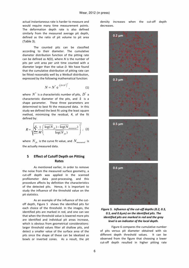
As an example of the influence of the cut-
off depth, Figure 5 shows the identified pits for
each choice of the threshold. In the images, the
identified pits are marked in red, and one can see
that when the threshold value is lowered more pits
are identified and individual pit areas increase,
which is obvious from geometrical considerations:
larger threshold values filter all shallow pits, and
detect a smaller value of the surface area of the
pits since the shape of these can be idealized as
bowls or inverted cones. As a result, the pit
density increases when the cut-off depth
decreases.
Figure 5. Influence of the cut-off depths (0.2, 0.3,
0.5, and 0.6m) on the identified pits. The
identified pits are marked in red and the gray
level is an indicator of the local depth.
Figure 6 compares the cumulative number
of pits versus pit diameter obtained with six
different depth threshold values. It can be
observed from the figure that choosing a lower
cut-off depth resulted in higher pitting rate
0.2 µm
0.3 µm
0.5 µm
0.6 µm

Wear, 2012 (in press)
7
probably due to the detection of surface roughness
as erroneous pits. And on the other hand, more
and more shallow pits were discarded with
increasing cut-off, resulting in loss of smallest pits
for further statistic analysis. Hence, it is important
to select the cut-off depth threshold such that a
statistically significant number of real, non-
overlapping pits can be identified. By comparing
the raw image of the pitted surface and the
detected pits at different cut-off depth, we
concluded that 0.3 μm cut-off is a reasonable
choice that captures most of visually discernable
pits. The 0.3 μm cut-off is also above the noise of
the virgin surface left after the final polish by the
0.01 μm diamond slurry. We present below results for 0.3 μm and 0.5 μm .
Figure 6. Influence of depth cut-off threshold on
the pitting rate. Data shown is for SS A2205 pitted
with 4000 psi cavitation jet for 1 minute.
Figure 7. Effect of various threshold levels on
pitting rate analysis for the three materials
studied.
Figure 7 shows the maximum pitting rates
(i.e. pitting rates for D ≥ 0.5m) for selected tested
materials and pressures as functions of the cutoff
depth value. The trend of detecting more number
of pits as the threshold decreases is common for
the two NAB samples and the SS sample. In this
study, based on the results obtained, a cut-off
depth of 0.3 µm selected as a good compromise.
Additionally, data for cut-off depth of 0.5 µm is
also presented for comparison purposes.
6 Effect of Cavitation Intensity (Jet
Pressure) on Pitting Rate
We present here results of tests carried out
at different jet pressures varying from 700 psi to
7000 psi (or jet speeds from about 250 ft/s to 850
ft/s). As discussed earlier, the pitting test results
can be expressed by Weibull distributions with a
shape parameter, k, a characteristic diameter,
*D and a characteristic pitting rate, *N . The
effect of the jet pressure (or the cavitation
intensity) on these parameters and, as a
consequence, on the whole distribution function of
pitting rate versus pit diameter is investigated in
this section.
Figure 8 and Figure 9 show the pit
distributions at different jet speeds for stainless
steel A2205 samples respectively for cutoff depths
in the analysis of the pits of 0.3 µm and 0.5 µm. In
all cases the jets were discharged at atmospheric
pressure. For all case, the Weibull fits are
acceptable and cover the full range of pit sizes
including the larger diameter values, which
correspond to rare high intensity events. The shape
parameter, k, found to fit the data best was k= 0.74
for the cutoff depth of 0.3 µm and k=0.85 for the
cutoff depth of 0.5 µm.
Figure 10 and Figure 11 show that curve fits
with k=1.0, as used in [33], fit well the data for the
smaller diameters but deviate for the more intense
event which produce the larger diameter pits.
Figure 8: Cumulative pitting rate as a function of
pit diameter for different values of the jet
pressure on duplex stainless steel A2205 (cut-off
depth: 0.3 µm). Curve fits correspond to the three-
parameter Weibull distributions,
*exp / * ,k
N N D D , with all three
parameters fitted.

Wear, 2012 (in press)
8
Figure 9: Cumulative pitting rate as a function of
pit diameter for different values of the jet
pressure on duplex stainless steel A2205 (cut-off
depth: 0.5 µm). Curve fits correspond to the three-
parameter Weibull distributions,
*exp / * ,k
N N D D with all three
parameters fitted.
Figure 10: Cumulative pitting rate as a function of
pit diameter for different values of the jet
pressure on duplex stainless steel A2205 (cut-off
depth: 0.3 µm). Curve fits correspond to Weibull
distributions, *exp / * ,k
N N D D with two
parameters fitted and k=1.
Figure 12 and Figure 13 show the two
characteristic parameters the pit diameter, D*, and
the characteristic pitting rate, N*, as functions of
the jet pressure. One can easily see that the
characteristic pit size increases with the jet
pressure or speed. This trend can be fitted with a
power law indicating that the diameter increases
as the jet pressure to the power 0.877 (or the jet
velocity to the power 1.75). Similarly, the
characteristic pitting rate increases as the jet
pressure to the power 1.25 (or the jet velocity to
the power 2.5). This high power can be explained
by the fact that increasing the jet pressure or
speed both brings in more collapsing bubbles and
increases the number of more intense cavitation
bubble collapse events. Hence, the characteristics
pit size and the pitting rate obtained can be used
as a measure of the intensity level of the cavitating
field.
Figure 11: Cumulative pitting rate as a function of
pit diameter for different values of the jet
pressure on duplex stainless steel A2205 (cut-off
depth: 0.5 µm). Curve fits correspond to
parameter Weibull distributions,
*exp / * ,k
N N D D with two parameters
fitted and k=1.
Figure 12. Fitted characteristic parameter, *D
for different values of jet pressure on duplex
stainless steel A2205 (cut-off depth: 0.3 µm).
Here, k is fixed at 0.70.
Figure 13. Fitted characteristic parameter, *N
for different values of jet pressure on duplex
stainless steel A2205 (cut-off depth: 0.3 µm). Here
is k is fixed at 0.70.
Wear, 2012 (in press)
9
7 Dependence on Materials
This section considers the differences
between the pitting results between the three
considered materials: Aluminum alloy, Nickel
Aluminum Bronze, and Duplex Stainless Steel.
Figure 14 to Figure 16 show both the cumulative
pitting rates as a function of pit diameters for
different values of jet pressure and the
corresponding Weibull fits with k = 0.7. For all
cases, the cut-off depth was chosen to be 0.30 μm.
One can see that the value of k=0.7 can be
considered appropriate for all three materials.
Figure 16 includes also data for the ultrasonic
cavitation method following the G32 standard. The
pitting results from two different durations of G32
tests (1 min. vs. 3 min.) produced very close pitting
rates. This means during this short time, pit
overlapping did not happen. The pitting statistics
from G32 tests were close to that of 1000 psi jet
cavitation. The G32 data also follows the same
functional fit trend.
Using the idea that pitting rates of a specific
material in a given erosive cavitation field can be
described by the two parameters N* and D*, we
can look at the evolution of these two parameters
with both the intensity of the erosive field and the
change in material. Figure 17 shows the evolution
of N*, the characteristic pitting rate, with the jet
pressure for the three materials. We can infer from
Figure 18 that the characteristic pit size of NAB is
larger compared to that of A2205 for the same
erosive filed of load pressures, indicating that
A2205 is more resistant to plastic deformation,
within the test duration used in this study. This is
correlated well with the yield stress values of the
two materials as shown in Table 1. These initial
plastic deformations are not necessarily directly
related to the cavitation erosion resistance of the
materials.
Similarly Figure 18 shows the variations of
the characteristic pit size with both the intensity of
the erosive field and the change in material. Here
too, it is clear that the pit size increases with the
jet pressure increases. The value of D* increases
almost linearly mildly with the jet pressure
(between ΔP0.5
and ΔP1.5
), while the values of N*
increase much more drastically with ΔP, i.e. up to
ΔP4.5
depending on materials. This again highlights
that the higher velocity jet cavitation field
generates much larger cavitation pressure pulses
on the material surface thus making a much larger
number of these pulses active in generating pits.
On the other hand it seems as if the amplitude of
the highest pulses increases in a more moderate
way with the jet pressure making the size of the
pits increase only almost linearly with the pressure.
8 Normalization of Results
The fact that all cumulative pitting rate data
seems to follow the same general trends can be
clearly illustrated by representing on the same plot
all data from all tests after normalizing each
cumulative pitting rate data with its corresponding
characteristic pitting rate, N*, and after
normalizing each pit diameter with the
characteristic pit diameters, D*, corresponding to
the combination material/jet pressure. As shown in
Figure 19, all non-dimensional data is very clearly
fitted with the selected Weibull function,
**
kD
DN N e
, independent of the considered
material and the jet operating conditions. The
figure shows two selected values of k: k=1.0, which
was used in previous work [33] and fits well small
diameter pits but not the larger diameter pits, and
k=0.7, which was found here to be more
appropriate over the full range of diameters.
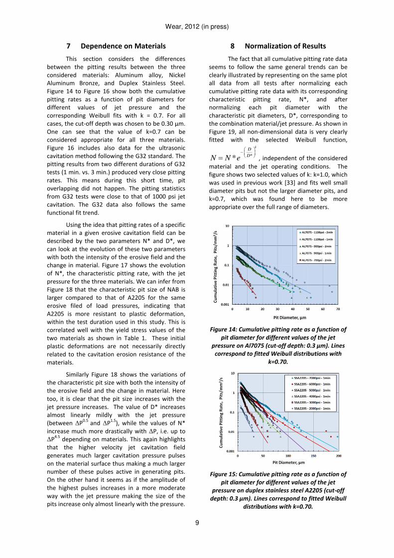
Figure 14: Cumulative pitting rate as a function of
pit diameter for different values of the jet
pressure on Al7075 (cut-off depth: 0.3 µm). Lines
correspond to fitted Weibull distributions with
k=0.70.
Figure 15: Cumulative pitting rate as a function of
pit diameter for different values of the jet
pressure on duplex stainless steel A2205 (cut-off
depth: 0.3 µm). Lines correspond to fitted Weibull
distributions with k=0.70.

Wear, 2012 (in press)
10
Figure 16: Cumulative pitting rate as a function of
pit diameter for different values of the jet
pressure on NAB (cut-off depth: 0.3 µm). Lines
correspond to fitted Weibull distributions with
k=0.70.
Figure 17. Comparison of fitted characteristic
parameter, *N for different values of jet
pressure.
Figure 18. Comparison of the pits characteristic
diameter, *D , for different values of the
cavitation erosive jet pressure.
Figure 19. Normalized pitting rate, N/N*, vs.
normalized pit diameter, D/D*, for two values of
the fitting function shape factor k=1.0 (top) and
k=0.7 (bottom).
The coverage rate β, i.e. the fraction of surface
covered by all pits whose diameter is larger than a
given value D, can be computed using Eq. 1:
k
2
D
2 k 1 u
D / D*
dN D( D ) dD
dD 4
kN * D* u e du
4
(3)
It can be shown that this β(D) function presents a
maximum for a particular pit diameter close to
3.6 D* in the case k 0.7 . This particular pit
diameter can then be considered as that of the pits
which contribute most to the coverage of the
pitted surface. This particular pit diameter
increases from about 13 µm (at 2000 psi) to 33 µm
(at 7000 psi) in the case of stainless steel A2205 as
deduced from Fig. 20. These values are somewhat
smaller than those given in [33]. This is most likely
ˆˆ
67.2%
DN e
Scatter
0.7ˆˆ
12.1%
DN e
Scatter
Wear, 2012 (in press)
11
due to an overall smaller length scale of the flow,
even though both flows are not geometrically
similar.
If all pits are included in the analysis, i.e. if the
integral in Eq. 3 is computed from D/D* = 0 to
infinity, the total coverage rate is (still in the case
k 0.7 ):
2 2k(0 ) 7.18 N * D* 4N * D*
4
(3)
The inverse of this total coverage rate,
1 / (0 ) , has the unit of a time and can be
interpreted as the coverage time, i.e. the time
necessary for the surface to be covered just one
time by the pits. This typical time varies between
about 2.7 hours (at 2000 psi) and 8 min (at
7000 psi) in the case of stainless steel A2205. This
time is one of the most relevant characteristic
times of the erosion process since several
coverages will actually be needed before complete
hardening of the material surface and the
subsequent inception of mass loss. Even though
the required number of coverages depends upon
the level of cavitation in terms of amplitude of
impact loads, most characteristic times of the
erosion process (such as the incubation time) are
expected to be strongly correlated to this coverage
time.
9 Pit Depth and Pit Volume
The volumes of the pits can be correlated
to their equivalent diameter based on the surface
area as shown in Figure 20, which presents all
individual pits for the duplex stainless steel A2205
samples at the different jet pressures considered.
The volumes are calculated based on the full 3D
geometry with no assumptions on pit shape, such
as axisymmetry or other. The left curve is based on
the cutoff depth of 0.3m, while the right curve
uses 0.5 m. Both figures show that the pit
volumes vary like the equivalent diameter raised to
the power 2.1, instead of say to the power 3, which
would be expected if the pits were hemispherical.
This does not depend significantly upon the depth
threshold used and the jet pressures in the present
range of investigation. This result is also recovered
for all materials tested and for all erosion
intensities both with the jets and the ultrasonic
cavitation, as illustrated in Figure 21.
Figure 20: Pit volume as a function of pit diameter
for different values of the jet pressure on duplex
stainless steel A2205. Left: Cut-off depth: 0.3 µm,
Righ: cut-off depth: 0.5 µm. The fit lines
correspond to 2.10.26 D (top) and 2.10.34 D
(bottom).
Figure 21: Pit volume as a function of pit diameter
for all materials tested and for different cavitation
mechanisms.
The small 2.1 exponent, i.e. 2.1
DV
indicates that the plastic deformation is actually
much wider than deep, i.e. very shallow. This is
illustrated in Figure 22 which shows pit depths
over pit diameters, or shape ratio, as a function of
pit diameter. The figure also shows the results for
the two cutoff depth values: 0.3m (left) and 0.5
m (right). The choice of the threshold did not
influence the shape factor too much. Figure 22 left
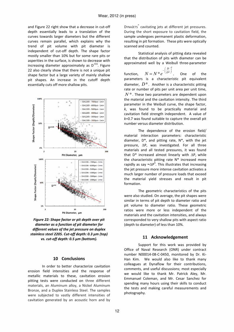
Wear, 2012 (in press)
12
and Figure 22 right show that a decrease in cut-off
depth essentially leads to a translation of the
curves towards larger diameters but the different
curves remain parallel, which explains why the
trend of pit volume with pit diameter is
independent of cut-off depth. The shape factor
mostly smaller than 10% but for some rare pits or
asperities in the surface, is shown to decrease with
increasing diameter approximately as D-0.6
. Figure
22 also clearly show that there is not a unique pit
shape factor but a large variety of mainly shallow
pit shapes. An increase in the cutoff depth
essentially cuts off more shallow pits.
Figure 22: Shape factor or pit depth over pit
diameter as a function of pit diameter for
different values of the jet pressure on duplex
stainless steel 2205. Cut-off depth: 0.3 µm (top)
vs. cut-off depth: 0.5 µm (bottom).
10 Conclusions
In order to better characterize cavitation
erosion field intensities and the response of
metallic materials to these, cavitation erosion
pitting tests were conducted on three different
materials, an Aluminum alloy, a Nickel Aluminum
Bronze, and a Duplex Stainless Steel. The samples
were subjected to vastly different intensities of
cavitation generated by an acoustic horn and by
DYNAJETS® cavitating jets at different jet pressures.
During the short exposure to cavitation field, the
sample undergoes permanent plastic deformation,
resulting in pit formation. These pits were optically
scanned and counted.
Statistical analysis of pitting data revealed
that the distribution of pits with diameter can be
approximated well by a Weibull three-parameter
function, ** .
kD
DN N e
One of the
parameters is a characteristic pit equivalent
diameter, *D . Another is a characteristic pitting
rate or number of pits per unit area per unit time,
*N . These two parameters are dependent upon
the material and the cavitation intensity. The third
parameter in the Weibull curve, the shape factor,
k, was found to be practically material and
cavitation field strength independent. A value of
k=0.7 was found suitable to capture the overall pit
number versus diameter distribution.
The dependence of the erosion field/
material interaction parameters: characteristic
diameter, D*, and pitting rate, N*, with the jet
pressure, ΔP, was investigated. For all three
materials and all tested pressures, it was found
that D* increased almost linearly with ΔP, while
the characteristic pitting rate N* increased more
rapidly as say ~ΔP5. This illustrates that increasing
the jet pressure more intense cavitation activates a
much larger number of pressure loads that exceed
the material yield stresses and result in pit
formation.
The geometric characteristics of the pits
were also studied. On average, the pit shapes were
similar in terms of pit depth to diameter ratio and
pit volume to diameter ratio. These geometric
ratios were more or less independent of the
materials and the cavitation intensities, and always
corresponded to very shallow pits with aspect ratio
(depth to diameter) of less than 10%.
11 Acknowledgement
Support for this work was provided by
Office of Naval Research (ONR) under contract
number N00014-08-C-0450, monitored by Dr. Ki-
Han Kim. We would also like to thank many
colleagues at Dynaflow for their contributions,
comments, and useful discussions; most especially
we would like to thank Mr. Patrick Aley, Mr.
Emmanuel Coleman, and Mr. Cesar Sanchez for
spending many hours using their skills to conduct
the tests and making careful measurements and
photography.
Wear, 2012 (in press)
13
Nomenclature
References
1. Thiruvengadam, A., “Handbook of Cavitation Erosion,” Hydronautics Technical Report 7301-
1, 1974.
2. Eisenberg, P., Preiser, H.S., and
Thiruvengadam, A., “On the Mechanisms of Cavitation Damage and Methods of
Protection,” Transac. Soc. Naval Architects 73,
241–286, 1965.
3. Pereira, F., Avellan, F., Dupont, Ph.,
“Prediction of Cavitation Erosion: An Energy
Approach,” Journal of Fluids Engineering, 120, 719-727, 1998.
4. Choi, J.-K., Chahine, G.L., Frederick, G.S., Aley,
P., “Evaluation of Coatings Provided by NSWCCD for Their Resistance to Cavitation
Generated by Cavitating DYNAJETS®”, Report
No. 2M7018-NSWC-1, DYNAFLOW, INC. Sep.
2007.
5. Chahine, G.L., "Cavitation Cloud Theory," Proc.
14th Symposium on Naval Hydrodynamics,
Ann Arbor, Michigan, National Academy Press,
pp. 165-194, Washington, D.C., 1983.
6. Chahine, G. L. and Duraiswami, R., "Dynamical
Interactions in a Bubble Cloud", Journal of
Fluids Engineering, Vol.114, p.680-686, 1992.
7. Morch, K.A., “Dynamics of Cavitation Bubbles
and Cavitating Liquids”, Treatise on Materials
Science and Technology Vol. 16: 309-355,
1979.
8. Morch, K.A., “Concerted Collapse of Cavities in
Ultrasonic Cavitation,” Proc. Acoustic Cavitation Meeting, London, 62, 1977.
9. D'Agostino, L. and Brennen, C.E., “On the
Acoustical Dynamics of Bubble Clouds”, ASME
Cavitation and Polyphase Flow Forum,
Houston, 72-76, 1983.
10. Brennen, C.E., Cavitation and Bubble
Dynamics, Oxford University Press, New York,
Oxford, 1995.
11. Shimada, M., Kobayashi, T., Matsumuto, Y.,
“Dynamics of cloud cavitation and cavitation erosion”, Proc. the ASME/JSME Fluids
Engineering Division Summer Meeting, San
Francisco, CA, 1999.
12. Blake, J.R., Taib, B.B., Doherty, G., “Transient Cavities near Boundaries. Part I. Rigid
Boundary”, Journal of Fluid Mechanics, Vol.
170, pp.479-497, 1986.
13. Zhang, Duncan, H., Chahine, G.L., “The Final Stage of the Collapse of a Cavitation Bubble
near a Rigid Wall”, Journal of Fluid Mechanics,
Vol. 257, pp.147-181, 1993.
14. Lauterborn, W., Bolle, H., “Experimental investigations of cavitation-bubble collapse in
the neighbourhood of a solid boundary”, J.
Fluid Mech. 72, 391–399, 1975.
15. Chahine, G.L., Perdue, T.O., “Simulation of the Three-Dimensional Behavior of an Unsteady
large Bubble near a Structure”, Drops and
Bubbles, Third International Colloquium,
Monterey, CA, ed. Taylor G. Wang, pp.188-
199, 1988.
16. Lush, P.A., “Impact of a liquid mass on a perfectly plastic solid”, J. Fluid Mech. 135,
373–387, 1983.
17. Parsons, C.A. and Cook, S.S., “Investigation into causes of corrosion or erosion of
propellers”, J. Am. Soc. Naval Eng., 31, 536-
541, 1919.
18. Plesset, M.S. and Ellis, “On the mechanism of cavitation damage”, A.T., Trans. ASME, 77,
1055-1064, 1955.
19. Knapp, R.T., “Recent Investigations of the Mechanics of Cavitation and Cavitation
Damage”, Trans. ASME, 77, 1045-1054, 1955.
20. Knapp, R.T., “Accelerated Field Tests of Cavitation Intensity” Trans. ASME, 80, pp.91-
102, Jan. 1958.
21. Knapp, R.T., Daily, J.W., Hammitt, F.G.,
Cavitation, McGraw-Hill, London, 1970.
22. Dorey, J.M, Laperrousaz, E., Avellan, P.,
Dupont, P., Simoneau, R., Bourdon, P.,
“Cavitation Erosion Prediction on Francis Turbines – Part 3 Methodologies of
Prediction”, Hydraulic machinery and cavitation: proceedings of the XVIII IAHR
Symposium, ed. Cabrera, E., Espert, V.
Martinez, F., Vol. I, Kluwer Academic
Publishers, 1996.
23. Dular, M., Stoffel, B., Sirok, B., “Development of a cavitation erosion model”, Wear 261, 642-
655, 2006.
24. N. Berchiche, J.P. Franc, J.M. Michel, “A Cavitation Erosion Model for Ductile
Materials”, Proc. 4th International Symposium
on Cavitation, CAV2001, Pasadena, CA, Jun.
2001.
25. Mohamed Farhat, Paul Bourdon, Pierre
Lavigne, Raynald Simoneau, “The Hydrodynamic Aggressiveness of Cavitating
N Number of Pits #/mm2/s
*N Characteristic Number of Pits #/mm
2/s
Characteristic Time Parameter s
D Pit Diameter m
D * Characteristic Pit Diameter m
V Pit Volume 3m

Wear, 2012 (in press)
14
Flows in Hydro Turbines”, ASME Fluids Engineering Division Summer Meeting,
FEDSM'97, June 1997.
26. Billet, M.L., “The Specialist Committee on Cavitation Erosion on Propellers and
Appendages on High Powered/High Speed
Ships”, Final Report and Recommendations to the 24th ITTC, Proc. the 24th ITTC, Vol. II,
2005.
27. Stinebring, D.R., Holl, J.W, and Arndt, R.E.A.,
“Two Aspects of Cavitation Damage in the Incubation Zone: Scaling By Energy
Considerations and Leading Edge Damage”, Journal of Fluid Engineering, Vol. 102, pp. 481-
485, 1980.
28. Lee, M.K., Hong, S.M., Kim, G.H., Kim, K.H.,
Rhee, C.K., Kim, W.W., “Numerical correlation
of the cavitation bubble collapse load and
frequency with the pitting damage of flame
quenched Cu-9Al-4.5Ni-4.5Fe alloy”, Materials
Science & Engineering A (Structural Materials:
Properties, Microstructure and Processing)
425 (1-2):15-21.
doi:10.1016/j.msea.2006.03.039, 2006.
29. Hattori S., Takinami, M., Otani, T.,
“Comparison of cavitation erosion rate with
liquid impingement erosion rate”, Proc. the
7th International Symposium on Cavitation,
Ann Arbor, Michigan, USA, August, 2009.
30. Annual Book of ASTM Standards – Section 3
Material Test Methods and Analytical
Procedures, American Society for Testing and
Materials (ASTM), Vol. 03.02, 94-109 & 558-
571, 2010.
31. Chahine G.L., and Johnson V.E. Jr., “Mechanics
and Applications of Self-Resonating Cavitating
Jets”, International Symposium on Jets and
Cavities, ASME, WAM, Miami, FL, Nov. 1985.
32. Choi, J.-K., Jayaprakash, A., Chahine, G.L.,
“Scaling of Cavitation Erosion Progression with
Cavitation Intensity and Cavitation Source”, Wear 278-279, 53-61, 2011.
33. Franc, J.-P., Riondet, M., Karimi, A., Chahine,
G.L., “Material and Velocity Effects on
Cavitation Erosion Pitting”, Wear, Wear 274-
275: pp.248-259.
doi:10.1016/j.wear.2011.09.006, 2012.
34. March, P.A., “Evaluating the Relative
Resistance of Materials to Cavitation Erosion:
a Comparison of Cavitating Jet Results and
Vibratory Results”, Proc. Cavitation and Multiphase Flow Forum, ASME, Cincinnati,
1987.
35. Dynamic Behavior of Materials, Meyers, M. A.,
Wiley, p.300, 1994.
36. Carnelli, D., Karimi, A., Franc, J.-P.,
“Application of Spherical Nanoindentation to
Determine the Pressure of Cavitation Impacts
from Pitting Tests”, Journal of Material
Research, 27 (1), 91-99, 2011.
37. “MatWeb Material Property Data”, MatWeb
LCC, www.matweb.com, 2011.
38. Danzl, R., Helmli, F. S. Scherer, S., “Focus
Variation – A New Technology For High
Resolution Optical 3D Surface Metrology”, 10th Int. Conf. the Slovenian Society for Non-
Destructive Testing, Ljubljana, Slovenia,
September 2009.
View publication statsView publication stats


![Cavitating Flow Calculations for the E779A Propeller in ... · PDF filetest case corresponds to the cavitation-tunnel set-up and not the towing-tank set-up, also available in [2]](https://img.pdfslide.us/doc/110x75/5aadd11a7f8b9a6b308b4d9c/cavitating-flow-calculations-for-the-e779a-propeller-in-case-corresponds-to.jpg)


![Theoretical Analysis of Thermodynamic Effect of Cavitation ... · tion with Kato’s model. Tani and Nagashima [6]simulated the cavitating flow around a hydrofoil with cryogenic](https://img.pdfslide.us/doc/110x75/61092707975b3c45cb3d0d22/theoretical-analysis-of-thermodynamic-effect-of-cavitation-tion-with-katoas.jpg)


![Erosion of Grooved Surfaces by Cavitating Jet with ... · wall. There are few studies on the cavitation of oblique impingement on solid surfaces [24], and there have been no attempts](https://img.pdfslide.us/doc/110x75/5e93b6d24da0746c467f7e43/erosion-of-grooved-surfaces-by-cavitating-jet-with-wall-there-are-few-studies.jpg)