Numerical Analysis of Flow Around the Cavitating CAV2003 ...flow.me.es.osaka-u.ac.jp/cav2003/Papers/Cav03-OS-1-010.pdf · CAV03-OS-1-010 Fifth International Symposium on Cavitation

CAV03-OS-1-010 Fifth International Symposium on Cavitation (CAV2003)Osaka, Japan, November 1-4, 2003

Numerical Analysis of Flow Around the Cavitating CAV2003Hydrofoil

Spyros A. KinnasOcean Engineering Group

The University of Texas at Austin, [email protected]

Hong SunOcean Engineering Group


Hanseong LeeOcean Engineering Group


ABSTRACT

This paper addresses the steady fully wetted and cav-itating flows over the CAV2003 benchmark hydrofoil in-side a tunnel by using a viscous and inviscid interactivemethod. The non-linear analysis of the inviscid cavitat-ing hydrofoil flow is based on a potential-based Bound-ary Element Method(BEM), with the cavity shape deter-mined in an iterative manner until both the kinematic anddynamic boundary conditions are satisfied on the cavitysurface. The effects of viscosity on the cavitating flow areconsidered by applying a viscous and inviscid interactiveintegral boundary layer analysis on the compound foil sur-face, i.e. the combined cavity and hydrofoil surface. Thismethod ignores the two-phase flow near the cavity surface,treating the fluid/vapor interface as constant pressure, freestreamline and forcing the friction coefficient to be zero onthe cavity surface.

The fully wetted case is performed using the vis-cous/inviscid coupling model (CAV2DBL), and comparedwith the turbulence model of the commercial software(FLUENT). The cavitating cases of CAV2003 hydrofoilare accomplished via the inviscid nonlinear model. Theeffects of tunnel walls are considered in both the invis-cid modeling and viscous modeling by using the imagemethod.

NOMENCLATURE

C : chord length of the foilCD : drag coefficient,CD = Drag

1

2ρU2

∞C

CL : lift coefficient, CL = Lift1

2ρU2

∞C

Cf : friction coefficient,Cf = Friction force1

2ρU2

∞C

CP : pressure coefficient,CP = P−P∞

1

2ρU2

∞

h : cavity thickness normal to foil surfaceHk : kinematic shape factorHk = δ∗

θ

lD : cavity detachment point location nondimensionalizedby chord length~n : surface unit normal vector~qc : cavity surface velocity vectors : arc length along foil surfaceUe : magnitude of boundary layer edge velocityU∞ : magnitude of free stream velocityα: inflow angle of attackδ∗ : boundary layer displacement thicknessθ: boundary layer momentum thicknessσ : cavitation number,σ = P∞−Pv

1

2ρU2

∞

φ : perturbation potential

INTRODUCTION

In recent decades, a lot of numerical methods havebeen developed to treat the wetted and cavitating flowsaround airfoils, hydrofoils and ship propellers. Specially,boundary element method (BEM) has been found to be acomputationally efficient, robust and versatile tool for theinviscid analysis of cavitating flows around arbitrary ge-ometries in two or three dimensions.

[Kinnas and Fine 1991, 1993b; Fine and Kinnas1993] have developed a non-linear potential based bound-ary element method for the analysis of partially or supercavitating flows around two- and three-dimensional hydro-foils. Their method was extended to predict face cavitationand search for cavity detachment on three-dimensional hy-drofoils and propellers by [Kinnas 1998]. In addition, themethod for cavity prediction over three-dimensional hy-


drofoils inside of a tunnel has been addressed in [Kinnas1998], in which the interaction between tunnel and hydro-foil was taken into account in an iterative manner.

A method coupling the inviscid flow solution witha boundary layer solution has been developed by [Drela1989]. His method was first applied for the analysis offully wetted flow around airfoils [Drela 1989] as wellas propeller blades [Hufford 1992; Hufford et al. 1994].Then the method was applied to partially cavitating hydro-foils by making the ”thin” cavity assumption [Villeneuve1993]. Recently, this method was extended to treat theflow around partially cavitating hydrofoils in fully non-linear theory, as well as the flow around super cavitatinghydrofoils [Kinnas et al. 1994b; Brewer and Kinnas 1997;Krishnaswamy 1999; Milewski 1997].

In the present paper, the viscous and inviscid couplingmethod is used to study the non-cavitating flow over theCAV2003 workshop testing foil. The numerical results arecompared with those computed by using FLUENTk − ωturbulence model. The effects of viscosity on the pressuredistribution and the force coefficients are also investigated.For the cavitating conditions, the three dimensional invis-cid potential-based boundary element method is employedto predict the cavity shapes and the detachment point loca-tions.

FORMULATION

Inviscid cavitating flow

A potential based boundary element method is ap-plied for the prediction of partial or super cavity on 2-Dhydrofoils using the inviscid non-linear theory. The de-tails of the numerical implementation for the partial or/andsuper cavity prediction are described in [Kinnas and Fine1993a,b; Kinnas 2001], and this section summarizes thetheoretical background of their inviscid non-linear method.

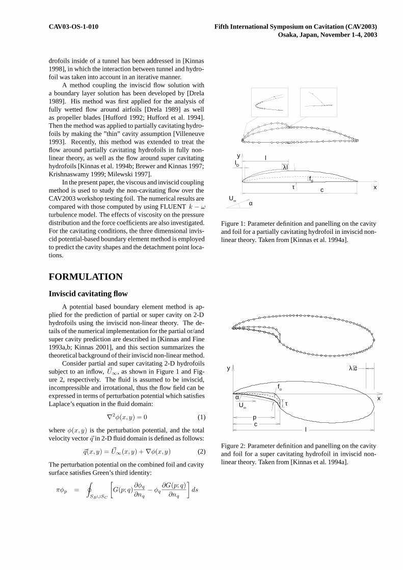
Consider partial and super cavitating 2-D hydrofoilssubject to an inflow,~U∞, as shown in Figure 1 and Fig-ure 2, respectively. The fluid is assumed to be inviscid,incompressible and irrotational, thus the flow field can beexpressed in terms of perturbation potential which satisfiesLaplace’s equation in the fluid domain:

∇2φ(x, y) = 0 (1)

whereφ(x, y) is the perturbation potential, and the totalvelocity vector~q in 2-D fluid domain is defined as follows:

~q(x, y) = ~U∞(x, y) + ∇φ(x, y) (2)

The perturbation potential on the combined foil and cavitysurface satisfies Green’s third identity:

πφp =

∮

SB∪SC

[

G(p; q)∂φq

∂nq

− φq

∂G(p; q)

∂nq

]

ds

y

x

llD

τf0

cU∞ α

λl

Figure 1: Parameter definition and panelling on the cavityand foil for a partially cavitating hydrofoil in inviscid non-linear theory. Taken from [Kinnas et al. 1994a].

fo

U∞

α

cp

l

τ

λ⋅c

x

y

Figure 2: Parameter definition and panelling on the cavityand foil for a super cavitating hydrofoil in inviscid non-linear theory. Taken from [Kinnas et al. 1994a].


−∮

SW

∆φW

∂G(p; q)

∂nq

ds (3)

whereG(p; q) = ln R(p; q) is the Green’s function in twodimensions,R(p; q) is the distance between a field point,p, and a point of integration,q, on the wetted foil, the cav-ity, and the wake surface.~n is the unit vector normal to thefoil or cavity surface.SB , SC , andSW denote the foil, thecavity, and the trailing wake surface, respectively.

The solutions of Eqn. 3 are uniquely determined byapplying the following boundary conditions on the bound-aries inside the fluid domain.

• The perturbed velocity vanishes at infinity:

∇φ = 0 (4)

• The kinematic boundary condition on the foil surfaceimplies that the flow is tangent to the wetted part ofthe foil surface:

∂φ

∂n= −~U∞ · ~n (5)

• Kutta condition requires the velocity at the foil trail-ing edge to be finite:

|∇φ| < ∞ (6)

By applying the Kutta condition, the dipole strengthin the trailing wake can be implicitly determined as apart of the solution of Eqn. 3. In the present work,Morino’s steady Kutta condition [Morino and Kuo1974] is applied as follows:

∆φW = φ+

T − φ−

T (7)

where∆φW is the potential jump on the wake sur-face. φ+

T andφ−

T are the potentials at the upper andlower sides of the foil trailing edge, respectively.

• The dynamic boundary condition on the cavity sur-face requires pressure to be constant and equal to thevapor (or cavity) pressure. The dynamic boundarycondition can be derived from the steady Bernoulli’sequation, and it requires to satisfy the following rela-tion between the magnitude of the cavity velocity andthe cavitation number.

|~qc| = |~U∞|√

1 + σ (8)

where~qc is the total velocity on the cavity surface;σis the cavitation number, which is defined as:

σ =p∞ − pv

1

2ρU2

∞

(9)

wherepv is the vapor (or cavity) pressure. By inte-grating Eqn. 8 along the cavity surface, the potentialon the cavity surface is obtained as follows:

φ(s) = φ(0) − ~U∞ · ~n + s|~U∞|√

1 + σ (10)

wheres is the arclength along the cavity surface mea-sured from the cavity leading edge, andφ(0) is thepotential at the leading edge of the cavity.

• The pressure condition at the cavity trailing edge isexpressed as:

|~qtr| = |~U∞|√

1 + σ [1 − f(x)] (11)

where~qtr is the velocity vector over a transition re-gion of lengthλ at the end of the cavity, andf(x)is an algebraic function defined in [Kinnas and Fine1993a,b]. Eqn. 11 corresponds to a pressure recov-ery cavity termination model [Lemonnier and Rowe1988], and is applied for the analysis of the partiallycavitating flow. The ”end parabola” model [Fine1992; Kinnas and Fine 1993a] which is the variationof the Riabouchinsky “end plate” model is applied forsuper cavitating flow.

• Cavity closure condition requires the cavity thicknessto be zero at the cavity trailing edge:

h(sL) =1

|~qc|

∫ sL

0

[

~U∞ · ~n +∂φ

∂n

]

ds = 0 (12)

whereh is the cavity thickness normal to the foil sur-face, andsL is the total arclength along the cavity sur-face from the cavity leading edge to its trailing edge.

In the current 2-D model, the cavity surface is deter-mined in an iterative manner for the known cavity detach-ment point location,lD, and the cavity length,lCAV . Thecavity surface is updated until both the kinematic and thedynamic boundary conditions are satisfied on the cavitysurface [Kinnas and Fine 1991, 1993b]. In the first itera-tion, the foil surface under the cavity is taken to be the cav-ity shape for partially cavitating hydrofoils, and the cavityshape from linear theory is taken to be the cavity shape forsuper cavitating hydrofoils.

Modeling of 2-D cavitating flow using 3-DBoundary Element Method

A three-dimensional low-order boundary elementmethod is applied for the analysis of the cavitating flowaround 2-D hydrofoil with tunnel wall effects. [Bal andKinnas 2003] verified this method by reproducing the 2-Dcavity shape on the hydrofoil inside of a wave tunnel us-ing 3-D boundary element method. They had panelled the


tunnel walls to follow the hydrofoil geometry, and the gapbetween foil ends and tunnel walls was set to be zero.

In the present work, the tunnel and cavitating hydro-foil problems are solved separately, and the interaction be-tween them is taken into account in an iterative mannerthrough the induced potential of each on the other.

Viscous model for fully wetted flow

By assuming that the viscous flow is confined withina thin boundary layer on the foil and the wake surface,the effect of viscosity on the inviscid solution is includedby coupling a boundary layer solver [Drela 1989] with apotential solver. The boundary layer is taken into accountas lots of ”blowing” sources with their strengthsσ definedas [Kinnas et al. 1994b]:

σ =d(Ueδ

∗)

ds(13)

wheres is the arclength along the foil,Ue is the velocityat the edge of the viscous boundary layer, andδ∗ is thedisplacement thickness. The inviscid flow is coupled withthe viscous flow via the wall transpiration model whichgives the edge velocityUe in terms of the inviscid edgevelocity,U inv

e , and the mass defect term,m = Ueδ∗,

Ue = U inve + εUeδ

∗ (14)

whereε is a geometry dependent operator. The discretizedversion ofε is given in [Drela 1989; Hufford et al. 1994].

For a givenUe distribution, the parameters for thelaminar or turbulence boundary layer can be determinedfrom the boundary layer equations. First, the boundarylayer equations are solved with the inviscid edge veloc-ity distribution. Onceδ∗ is solved,Ue will be updatedvia Eqn. 14, and then the boundary layer equations aresolved again. This process continues until the convergenceis achieved.

Viscous-inviscid model coupling for cavitatinghydrofoil

For cavitating hydrofoil, the viscous flow in the vicin-ity of cavity is assumed to be confined to a thin boundarylayer, that is, the boundary layer displacement thickness isassumed to be small. The two-phase flow near the cavitysurface is ignored. The fluid/vapor interface is treated asa constant pressure free-streamline, and the friction coeffi-cientCf is set to be zero on the cavity surface [Kinnas et al.1994b]. The boundary conditions are now applied on thecompound foil surface (the combined ”nonlinear” cavityand foil surface), which is solved from the inviscid non-linear cavity theory. Then the boundary layer equationsare integrated along the non-linear cavity and foil surface.

The coupling method of the inviscid model with the vis-cous model is same as that of the fully wetted flow.

For the partially cavitating flow, the viscosity largelydecreases the cavity length and volume for fixed cavitationnumber and angle of attack, and increases the cavity lengthand volume for fixed cavitation number and lift coefficient[Kinnas et al. 1994b; Brewer and Kinnas 1997].

For the super cavitating flow, the effect of viscosityon predicted cavitation number for given cavity extent isvery small and can be negligible [Kinnas et al. 1994b].

Cavitation detachment point

According to the criterion of Arakeri, Franc andMichel, the cavity detachment should occur downstreamof laminar separation where the shape factorH = 4. His defined asH = δ∗

θ, whereδ∗ is the boundary layer

displacement thickness, andθ is the boundary layer mo-mentum thickness. The numerical method was used in aniterative manner [Kinnas et al. 1994b; Brewer and Kinnas1997] until laminar separation occurred just ahead of thedetachment point.

Effect of tunnel walls

The effects of tunnel walls are considered in both theinviscid solver and the boundary layer solver by providingan adequate number of ”images” of sources and dipoles,which represent the foil, the cavity, and the boundary layerdisplacement thickness [Villeneuve 1993].

Validation test for fully wetted flow

The present numerical method is validated by com-paring the numerical results with those measured fromexperiment and computed by using the commercial codeFLUENT. The experiment was performed by [Brewer andKinnas 1997] in MIT variable pressure water tunnel whichhas a twenty-inch square test section. The foil used in theexperiment had a symmetric cross section, and the halfthickness form was given as the following expression:

y = c1x0.5 + c2x + c3x

1.5 + c4x2 (15)

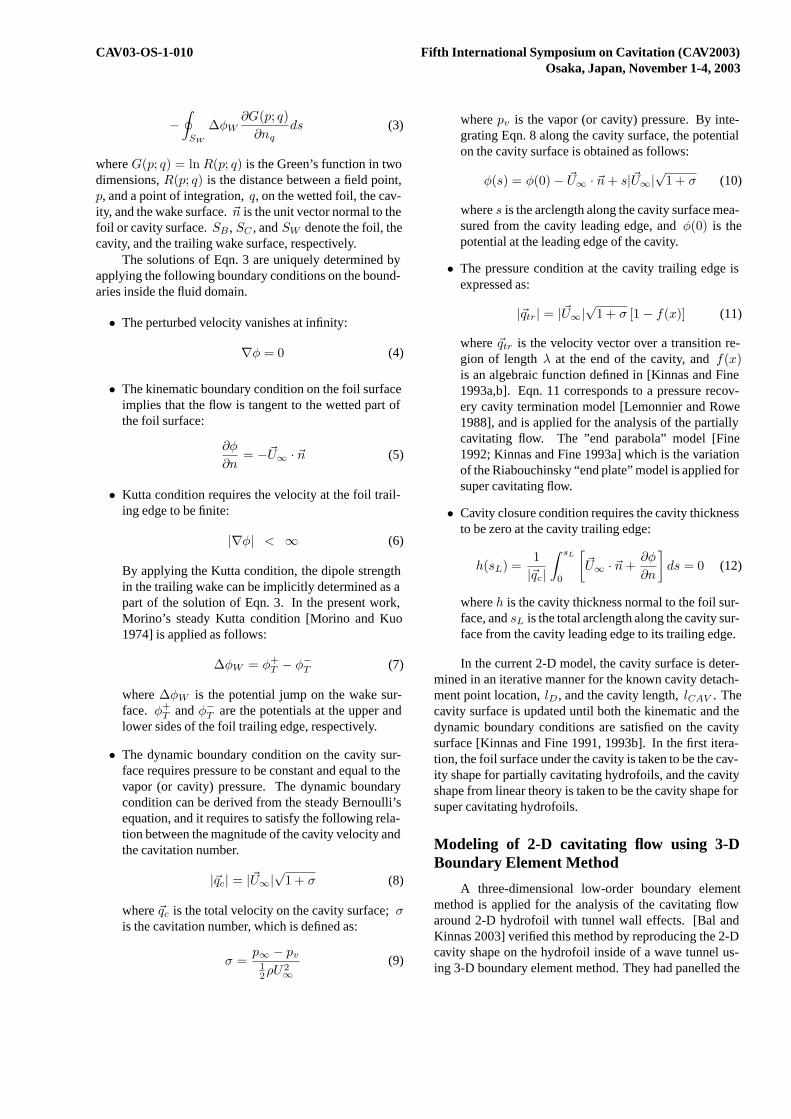
wherex = x/C andy = y/C , C is the chord length. Thecoefficients were given asc1 = 0.1787, c2 = −0.3997,c3 = 0.7611, andc4 = −0.5401. The foil chord lengthwasC = 305mm, and the maximum thickness to chordlength ratio wastmax/C = 0.12 at x = 0.485. The foilwas mounted in the middle of the tunnel as shown in Fig-ure 3. The inflow velocity was8m/s, and the foil wasplaced at an angle of attack ofα = 3.25o in the fully wet-ted flow. The tunnel had a turbulence level of1%, and aturbulent strip was placed at1

5chord on the pressure side

of the foil.


U∞

508mm

C = 305mm

Figure 3: Experiment setup of the heavy foil in MIT watertunnel. Fully wetted flow;U∞ = 6m/s; α = 3.25o.

X/C

-CP

0 0.25 0.5 0.75 1-1

-0.5

0

0.5

1

1.5

2

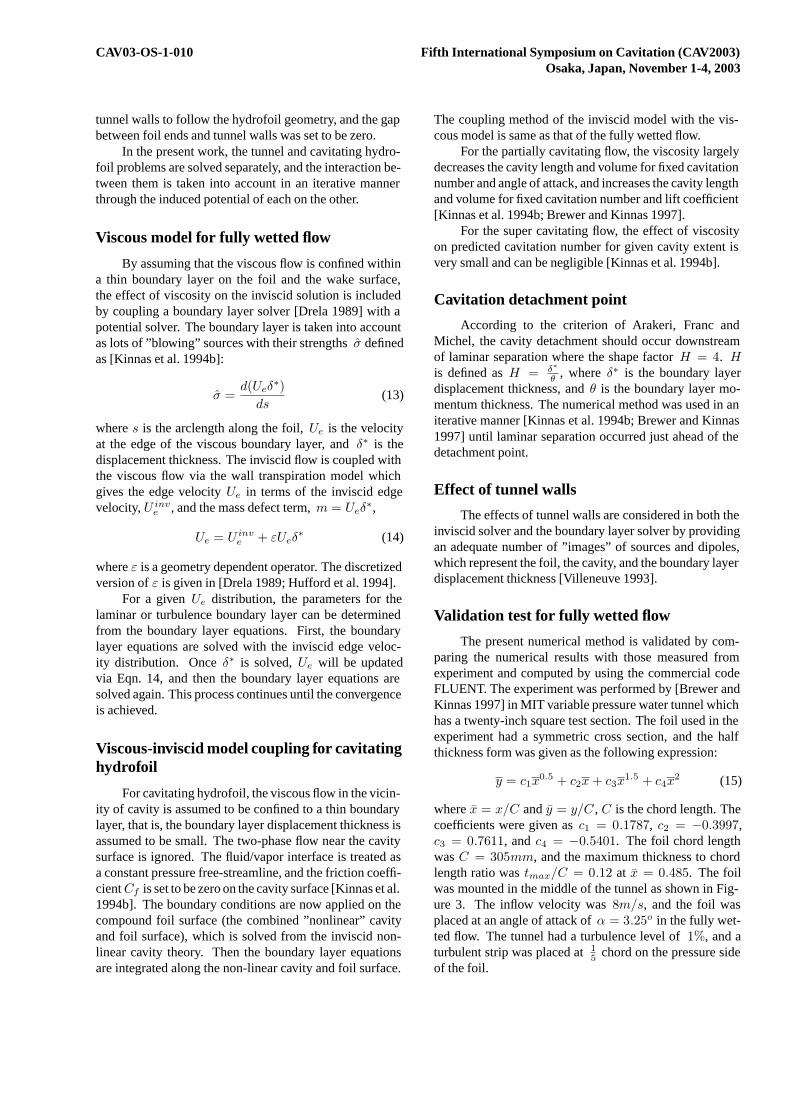
FLUENTCAV2DBL

Figure 4: Pressure distribution on the heavy foil surface.Fully wetted flow;U∞ = 6m/s; α = 3.25o.

The numerical calculations are performed byCAV2DBL with the inviscid, viscous/inviscid couplingmodel [Brewer and Kinnas 1996] and by FLUENT withthe k − ω turbulence model in the fully wetted flow.Figure 4 shows the comparison of pressure distributionson the foil surface predicted by using FLUENT andCAV2DBL. Since no separation is detected in FLUENTcalculation, the predicted pressure distributions from thetwo models are well compared with each other. Thecomputed lift coefficients using CAV2DBL with theinviscid, viscous/inviscid coupling model and FLUENTk − ω turbulence model are compared with that obtainedfrom experiment, as shown in Table 1. The viscous resultsfrom CAV2DBL and FLUENT are well compared withthe experimental measurements. The inviscid modelwithout the effect of viscosity predicts much higher liftcoefficient than those of viscous runs.

Table 1: The predicted lift coefficients using CAV2DBLand FLUENT. Fully wetted flow for the heavy foil;U∞ =6m/s; α = 3.25o.

CAV2DBL CAV2DBL FLUENT Experiment(inviscid) (viscous)

CL 0.4679 0.3668 0.3629 0.3619

RESULTS

Fully wetted flow

The numerical calculations for CAV2003 hydrofoilare performed in the case of non-cavitating flow byCAV2DBL with the inviscid, viscous/inviscid couplingmodel, and by FLUENT with thek −ω turbulence model.The tunnel height isH = 4C, and the tunnel turbulencelevel at the inlet is0.1%. The CAV2003 hydrofoil of chordlengthC = 0.1m is placed in the tunnel with an angle ofattack equal to7o. The inflow velocity isU∞ = 6m/s.ρ = 1000kg/m3 is the fluid density, and the fluid dynamicviscosity isµ = 1.0 × 10−3kg/m · s.

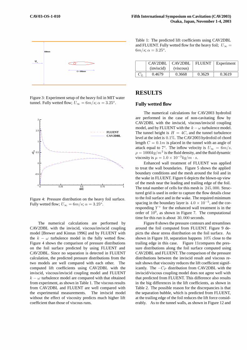
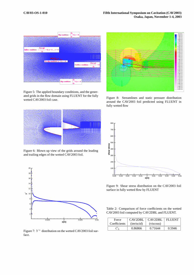
Enhanced wall treatment of FLUENT was appliedto treat the wall boundaries. Figure 5 shows the appliedboundary conditions and the mesh around the foil and inthe wake in FLUENT. Figure 6 depicts the blown-up viewof the mesh near the leading and trailing edge of the foil.The total number of cells for this mesh is245, 000. Struc-tured grid is used in order to capture the flow details closeto the foil surface and in the wake. The required minimumspacing in the boundary layer is4.0 × 10−5, and the cor-respondingY + for the enhanced wall treatment is in theorder of 100, as shown in Figure 7. The computationaltime for this run is about30, 000 seconds.

Figure 8 shows the pressure contours and streamlinesaround the foil computed from FLUENT. Figure 9 de-picts the shear stress distribution on the foil surface. Asshown in Figure 10, separation happens10% close to thetrailing edge in this case. Figure 11compares the pres-sure distributions along the foil surface computed usingCAV2DBL and FLUENT. The comparison of the pressuredistributions between the inviscid result and viscous re-sult shows that viscosity reduces the lift coefficient signif-icantly. The−CP distribution from CAV2DBL with theinviscid/viscous coupling model does not agree well withthat predicted from FLUENT. This difference also resultsin the big differences in the lift coefficients, as shown inTable 2. The possible reason for the discrepancies is thatthe separation bubble, which is predicted from FLUENT,at the trailing edge of the foil reduces the lift force consid-erably. As to the tunnel walls, as shown in Figure 12 and


∂(u,v,p)Outflow condition: = 0

∂y

No slip condition: u = 0, v = 0

∂uSlip condition: = 0, v = 0

∂y

∂uSlip condition: = 0, v = 0

∂y

∂(u,v,p)Inflow condition: = 0, u = U ∝ , v = 0

∂y

Figure 5: The applied boundary conditions, and the gener-ated grids in the flow domain using FLUENT for the fullywetted CAV2003 foil case.

Figure 6: Blown up view of the grids around the leadingand trailing edges of the wetted CAV2003 foil.

x(m)

y+

-0.025 0 0.025 0.05

2

4

6

8

10

12

14

16

18

20

Figure 7:Y + distribution on the wetted CAV2003 foil sur-face.

pressure1.60E+041.39E+041.18E+049.68E+037.58E+035.47E+033.37E+031.26E+03

-8.42E+02-2.95E+03-5.05E+03-7.16E+03-9.26E+03-1.14E+04-1.35E+04-1.56E+04-1.77E+04-1.98E+04-2.19E+04-2.40E+04-2.61E+04-2.82E+04-3.03E+04-3.24E+04-3.45E+04-3.66E+04-3.87E+04-4.08E+04-4.29E+04-4.51E+04-4.72E+04-4.93E+04-5.14E+04-5.35E+04-5.56E+04-5.77E+04-5.98E+04-6.19E+04-6.40E+04

Figure 8: Streamlines and static pressure distributionaround the CAV2003 foil predicted using FLUENT infully wetted flow

x(m)

shea

rstre

ss

-0.05 -0.04 -0.03 -0.02 -0.01 0 0.01 0.02 0.03 0.04 0.050

100

200

300

400

500

600

700

800

Figure 9: Shear stress distribution on the CAV2003 foilsurface in fully wetted flow by FLUENT

Table 2: Comparison of force coefficients on the wettedCAV2003 foil computed by CAV2DBL and FLUENT.

Force CAV2DBL CAV2DBL FLUENTCoefficients (inviscid) (viscous)

CL 0.86866 0.71644 0.5946


10%close to the trailing edge

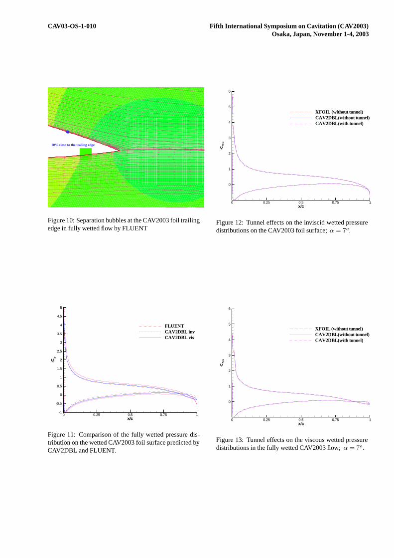
Figure 10: Separation bubbles at the CAV2003 foil trailingedge in fully wetted flow by FLUENT

x/c

-Cp

0 0.25 0.5 0.75 1-1

-0.5

0

0.5

1

1.5

2

2.5

3

3.5

4

4.5

5

FLUENTCAV2DBL invCAV2DBL vis

Figure 11: Comparison of the fully wetted pressure dis-tribution on the wetted CAV2003 foil surface predicted byCAV2DBL and FLUENT.

x/c

-CP

inv

0 0.25 0.5 0.75 1

0

1

2

3

4

5

6

XFOIL (without tunnel)CAV2DBL(without tunnel)CAV2DBL(with tunnel)

Figure 12: Tunnel effects on the inviscid wetted pressuredistributions on the CAV2003 foil surface;α = 7o.

x/c

-CP

vis

0 0.25 0.5 0.75 1

0

1

2

3

4

5

6

XFOIL (without tunnel)CAV2DBL(without tunnel)CAV2DBL(with tunnel)

Figure 13: Tunnel effects on the viscous wetted pressuredistributions in the fully wetted CAV2003 flow;α = 7o.


α / σ

l/C

0 0.2 0.4 0.6 0.80

0.5

1

1.5

2

2.5

σ = 0.8

σ = 0.4

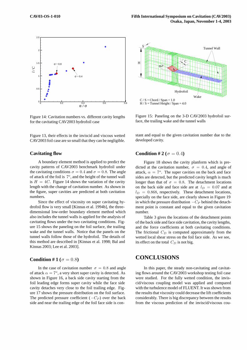
Figure 14: Cavitation numbers vs. different cavity lengthsfor the cavitating CAV2003 hydrofoil case

Figure 13, their effects in the inviscid and viscous wettedCAV2003 foil case are so small that they can be negligible.

Cavitating flow

A boundary element method is applied to predict thecavity patterns of CAV2003 benchmark hydrofoil underthe cavitating conditionsσ = 0.4 andσ = 0.8. The angleof attack of the foil is7o, and the height of the tunnel wallis H = 4C. Figure 14 shows the variation of the cavitylength with the change of cavitation number. As shown inthe figure, super cavities are predicted at both cavitationnumbers.

Since the effect of viscosity on super cavitating hy-drofoil flow is very small [Kinnas et al. 1994b], the three-dimensional low-order boundary element method whichalso includes the tunnel walls is applied for the analysis ofcavitating flows under the two cavitating conditions. Fig-ure 15 shows the paneling on the foil surface, the trailingwake and the tunnel walls. Notice that the panels on thetunnel walls follow those of the hydrofoil. The details ofthis method are described in [Kinnas et al. 1998; Bal andKinnas 2003; Lee et al. 2003].

Condition # 1 (σ = 0.8)

In the case of cavitation numberσ = 0.8 and angleof attackα = 7o, a very short super cavity is detected. Asshown in Figure 16, a back side cavity starting from thefoil leading edge forms super cavity while the face sidecavity detaches very close to the foil trailing edge. Fig-ure 17 shows the pressure distribution on the foil surface.The predicted pressure coefficient (−CP ) over the backside and near the trailing edge of the foil face side is con-

H

Tunnel Wall

Hydrofoil

Wake

C

S

C / S = Chord / Span = 1.0H / S = Tunnel Height / Span = 4.0

α

Figure 15: Paneling on the 3-D CAV2003 hydrofoil sur-face, the trailing wake and the tunnel walls

stant and equal to the given cavitation number due to thedeveloped cavity.

Condition # 2 (σ = 0.4)

Figure 18 shows the cavity planform which is pre-dicted at the cavitation number,σ = 0.4, and angle ofattack,α = 7o. The super cavities on the back and facesides are detected, but the predicted cavity length is muchlonger than that ofσ = 0.8. The detachment locationson the back side and face side are atlD = 0.07 and atlD = 0.868, respectively. These detachment locations,specially on the face side, are clearly shown in Figure 19in which the pressure distribution−CP behind the detach-ment point is constant and equal to the given cavitationnumber.

Table 3 gives the locations of the detachment pointsof the back side and face side cavitation, the cavity lengths,and the force coefficients at both cavitating conditions.The frictional CD is computed approximately from thewetted local shear stress on the foil face side. As we see,its effect on the totalCD is not big.

CONCLUSIONS

In this paper, the steady non-cavitating and cavitat-ing flows around the CAV2003 workshop testing foil casewere studied. For the fully wetted condition, the invis-cid/viscous coupling model was applied and comparedwith the turbulence model of FLUENT. It was shown fromthe results that viscosity could decrease the lift coefficientsconsiderably. There is big discrepancy between the resultsfrom the viscous prediction of the inviscid/viscous cou-


x / C

l/C

-0.5 -0.25 0 0.25 0.5

-0.1

0

0.1

0.2

0.3

σ = 0.8

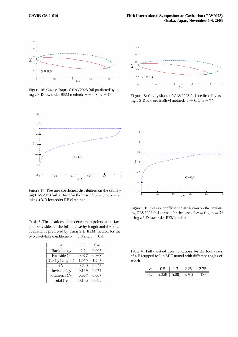
Figure 16: Cavity shape of CAV2003 foil predicted by us-ing a 3-D low order BEM method;σ = 0.8, α = 7o

x / C

-CP

0 0.2 0.4 0.6 0.8 1-1.5

-1

-0.5

0

0.5

1

1.5

σ = 0.8

Figure 17: Pressure coefficient distribution on the cavitat-ing CAV2003 foil surface for the case ofσ = 0.8, α = 7o

using a 3-D low order BEM method

Table 3: The locations of the detachment points on the faceand back sides of the foil, the cavity length and the forcecoefficients predicted by using 3-D BEM method for thetwo cavitating conditionsσ = 0.8 andσ = 0.4.

σ 0.8 0.4

BacksidelD 0.0 0.007FacesidelD 0.977 0.868

Cavity Lengthl 1.099 1.248CL 0.729 0.242

InviscidCD 0.139 0.073FrictionalCD 0.007 0.007

TotalCD 0.146 0.080

x / C

l/C

-0.5 -0.25 0 0.25 0.5

-0.1

0

0.1

0.2

0.3

σ = 0.4

Figure 18: Cavity shape of CAV2003 foil predicted by us-ing a 3-D low order BEM method;σ = 0.4, α = 7o

x / C

-CP

0 0.2 0.4 0.6 0.8 1-1.5

-1

-0.5

0

0.5

1

1.5

σ = 0.4

Figure 19: Pressure coefficient distribution on the cavitat-ing CAV2003 foil surface for the case ofσ = 0.4, α = 7o

using a 3-D low order BEM method

Table 4: Fully wetted flow conditions for the four casesof a B1cupped foil in MIT tunnel with different angles ofattack

α 0.5 1.3 2.25 -2.75

U∞ 5.228 5.08 5.086 5.198


XP/C

YP

/C

-1 -0.5 0 0.5 1

-0.6

-0.4

-0.2

0

0.2

0.4

0.6

Tunnel Wall

Tunnel Wall

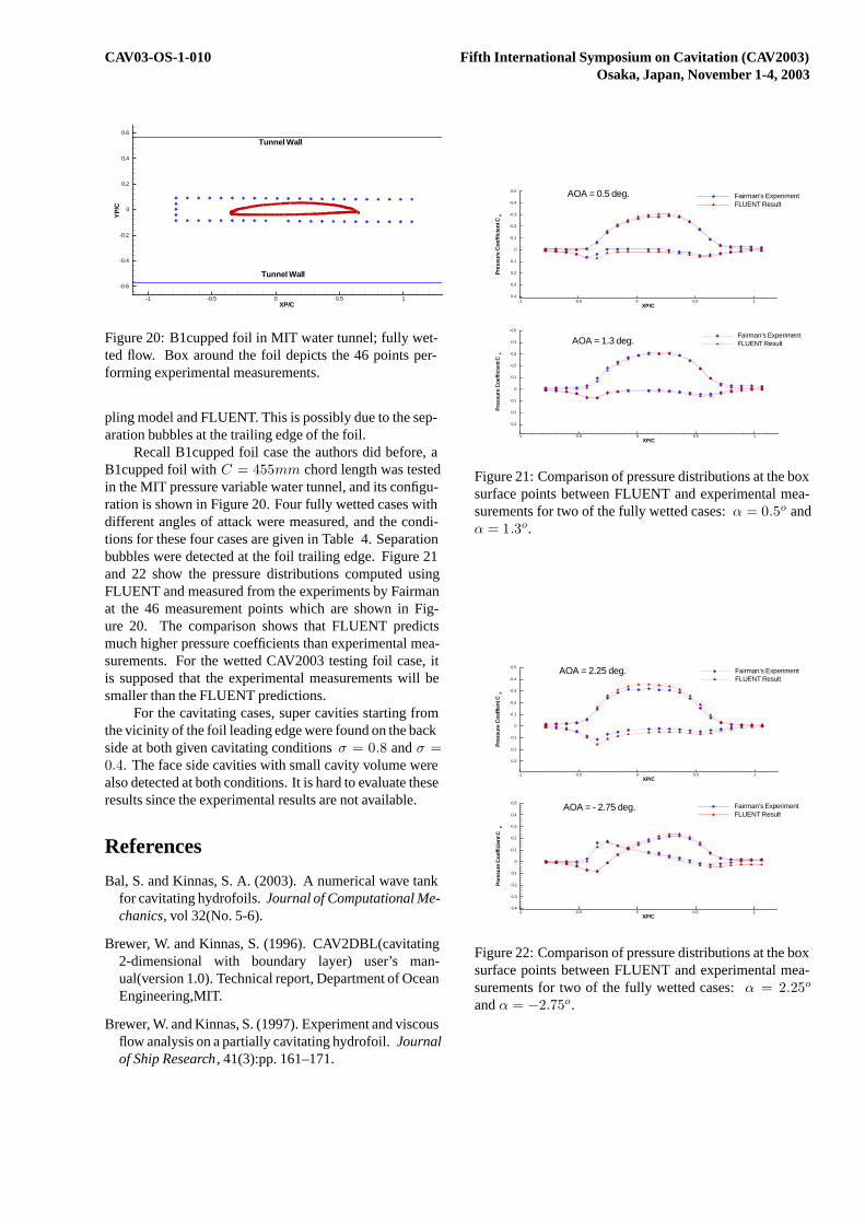
Figure 20: B1cupped foil in MIT water tunnel; fully wet-ted flow. Box around the foil depicts the 46 points per-forming experimental measurements.

pling model and FLUENT. This is possibly due to the sep-aration bubbles at the trailing edge of the foil.

Recall B1cupped foil case the authors did before, aB1cupped foil withC = 455mm chord length was testedin the MIT pressure variable water tunnel, and its configu-ration is shown in Figure 20. Four fully wetted cases withdifferent angles of attack were measured, and the condi-tions for these four cases are given in Table 4. Separationbubbles were detected at the foil trailing edge. Figure 21and 22 show the pressure distributions computed usingFLUENT and measured from the experiments by Fairmanat the 46 measurement points which are shown in Fig-ure 20. The comparison shows that FLUENT predictsmuch higher pressure coefficients than experimental mea-surements. For the wetted CAV2003 testing foil case, itis supposed that the experimental measurements will besmaller than the FLUENT predictions.

For the cavitating cases, super cavities starting fromthe vicinity of the foil leading edge were found on the backside at both given cavitating conditionsσ = 0.8 andσ =0.4. The face side cavities with small cavity volume werealso detected at both conditions. It is hard to evaluate theseresults since the experimental results are not available.

References

Bal, S. and Kinnas, S. A. (2003). A numerical wave tankfor cavitating hydrofoils.Journal of Computational Me-chanics, vol 32(No. 5-6).

Brewer, W. and Kinnas, S. (1996). CAV2DBL(cavitating2-dimensional with boundary layer) user’s man-ual(version 1.0). Technical report, Department of OceanEngineering,MIT.

Brewer, W. and Kinnas, S. (1997). Experiment and viscousflow analysis on a partially cavitating hydrofoil.Journalof Ship Research, 41(3):pp. 161–171.

XP/C

Pre

ssur

eC

oeffi

cien

tCp

-1 -0.5 0 0.5 1

-0.5

-0.4

-0.3

-0.2

-0.1

0

0.1

0.2

0.3

Fairman’s ExperimentFLUENT ResultAOA = 1.3 deg.

XP/C

Pre

ssur

eC

oeffi

cien

tCp

-1 -0.5 0 0.5 1

-0.5

-0.4

-0.3

-0.2

-0.1

0

0.1

0.2

0.3

0.4

Fairman’s ExperimentFLUENT Result

AOA = 0.5 deg.

Figure 21: Comparison of pressure distributions at the boxsurface points between FLUENT and experimental mea-surements for two of the fully wetted cases:α = 0.5o andα = 1.3o.

XP/C

Pre

ssur

eC

oeffi

cien

tCp

-1 -0.5 0 0.5 1

-0.5

-0.4

-0.3

-0.2

-0.1

0

0.1

0.2

0.3

0.4


AOA = - 2.75 deg.

XP/C

Pre

ssur

eC

oeffi

entC

p

-1 -0.5 0 0.5 1

-0.5

-0.4

-0.3

-0.2

-0.1

0

0.1

0.2

0.3


AOA = 2.25 deg.

Figure 22: Comparison of pressure distributions at the boxsurface points between FLUENT and experimental mea-surements for two of the fully wetted cases:α = 2.25o

andα = −2.75o.


Drela, M. (1989). XFOIL: An analysis and design systemfor low Reynolds number airfoils. InLecture Notes inEngineering (Volume 54, Low Reynolds Number Aero-dynamics), New York. Springer-Verlag.

Fine, N. and Kinnas, S. (1993). A boundary elementmethod for the analysis of the flow around 3-d cavitatinghydrofoils. Journal of Ship Research, 37:213–224.

Fine, N. E. (1992).Nonlinear Analysis of Cavitating Pro-pellers in Nonuniform Flow. PhD thesis, Department ofOcean Engineering, MIT.

Hufford, G. (1992). Viscous flow around marine propellersusing boundary layer strip theory. Master’s thesis, Mas-sachusetts Institute of Technology.

Hufford, G., Drela, M., and Kerwin, J. (1994). Vis-cous flow around marine propellers using boundary-layer strip theory.Journal of Ship Research, 38(1):pp.52–62.

Kinnas, S. (1998). The prediction of unsteady sheet cavi-tation. InThird International Symposium on Cavitation,Grenoble, France.

Kinnas, S. (2001). Lecture 1: Supercavitating 2-d hydro-foils: prediction of performance and design. InSpecialCourse on Supercavitating Flows, von Karman Institute,Brussels, Belgium.

Kinnas, S. and Fine, N. (1991). Non-Linear Analysis of theFlow Around Partially or Super-Cavitating Hydrofoilsby a Potential Based Panel Method. InBoundary Inte-gral Methods-Theory and Applications, Proceedings ofthe IABEM-90 Symposium, Rome, Italy, October 15-19,1990, pages 289–300, Heidelberg. Springer-Verlag.

Kinnas, S. and Fine, N. (1993a). MIT-PCPAN and MIT-SCPAN User’s Manual, Version 1.0 the Analysis of Par-tially Cavitating Hydrofoils.

Kinnas, S. and Fine, N. (1993b). A numerical nonlinearanalysis of the flow around two- and three-dimensionalpartially cavitating hydrofoils. Journal of Fluid Me-chanics, 254:151–181.

Kinnas, S., S., M., and W.H., B. (1994a). Non-linear anal-ysis of viscous flow around cavitating hydrofoils. InTwentieth Symposium on Naval Hydrodynamics, pages446–465, University of California, Santa Barbara, CA.

Kinnas, S. A., Lee, H. S., and Mueller, A. C. (1998). Pre-diction of propeller blade sheet and developed tip vortexcavitation. In22nd Symposium on Naval Hydrodynam-ics, pages 182–198, Washington, D.C.

Kinnas, S. A., Mishima, S., and Brewer, W. H. (1994b).Nonlinear analysis of viscous flow around cavitating hy-drofoils. In Twentieth Symposium on Naval Hydrody-namics, pages 446–465, University of California, SantaBarbara.

Krishnaswamy, P. (1999). Re-entrant jet and viscous flowmodeling for partially cavitating hydrofoils. Techni-cal Report No. 99-3, Ocean Eng. Group, Department ofCivil Engineering, UT Austin.

Lee, H. S., Kinnas, S. A., Gu, H., and Natarajan, S. (2003).Numerical modeling of rudder sheet cavitation includ-ing propeller/rudder interaction and the effects of a tun-nel. In CAV2003: Fifth International Symposium onCavitation, Osaka, Japan.

Lemonnier, H. and Rowe, A. (1988). Another approach inmodelling cavitating flows.Journal of Fluid Mechanics,vol 195.

Milewski, W. (1997). Three-dimensional viscous flowcomputations using the integral boundary integral equa-tions simultaneously coupled with a low order panelmethod. PhD thesis, M.I.T., Department of Ocean En-gineering.

Morino, L. and Kuo, C.-C. (1974). Subsonic PotentialAerodynamic for Complex Configurations : A GeneralTheory.AIAA Journal, vol 12(no 2):pp 191–197.

Villeneuve, R. (1993). Effects of viscosity on hydrofoilcavitation. Master’s thesis, Massachusetts Institute ofTechnology.

Documents

Numerical Analysis of Flow Around the Cavitating CAV2003 ...flow.me.es.osaka-u.ac.jp/cav2003/Papers/Cav03-OS-1-010.pdf · CAV03-OS-1-010 Fifth International Symposium on Cavitation