Scale variation of GPS time series Markku Poutanen, Jorma Jokela, Matti Ollikainen, Hannu Koivula, Mirjam Bilker, Heikki Virtanen Finnish Geodetic Institute Geodeetinrinne 2, FIN-02430 Masala Finland Markku.Poutanen@fgi.fi Abstract. We give an overview of time series analyses of permanent GPS stations using solutions of the IGS and FinnRef® networks. Lomb periodograms show in most cases a statistically significant annual period both in station coordinates and inter-station distances. In regional networks the scale of the whole network changes periodically, and in some cases there is also a secular trend. There are several possible causes of scale variations, which may not be separable in the data. These include computational artefacts, periodic systematic errors in satellite orbits, signal path delay variations, and geophysical causes like loading and postglacial rebound. We discuss possible reasons, their significance, and their consequences on high-precision GPS observations. Additional constraints, e.g. time series from the superconducting gravimeter, are also discussed. Keywords. GPS time series, periodic variations ________________________________________

1 Introduction

The Finnish permanent GPS network FinnRef® consists of 13 GPS stations. The network is the backbone of the Finnish realisation of the EUREF frame, referred to as EUREF-FIN. Four stations in the FinnRef network belong to the EUREF permanent GPS-network (EPN), and one station belongs to the network of the International GPS Service (IGS). Through these stations FinnRef® creates a seamless connection to the global reference frames. The observations obtained by FinnRef® stations can be used for studying the geodynamics of the Earth’s crust (Fig. 1).

All FinnRef® stations are also used in the computation of the joint Nordic GPS network in the BIFROST (Baseline Inferences for Fennoscandian Rebound Observations, Sea Level and Tectonics) project (Milne et al., 2001, Scherneck et al., 2002).

Currently we have a seven year GPS time series. Quite soon after the beginning it became obvious that there were both seasonal and short term variations. Because one of the tasks was to measure

the land uplift rate, we had to take the variation into account. In the worst case it could lead to poor results or even misinterpretation, as demonstrated in Fig. 2.

The variation is visible both in the vertical component and in inter-station distances. In distances the amplitude of the variation depends on the vector length, thus leading us to consider the phenomenon as a possible scale error.

Fig. 1. Finnish permanent GPS network, FinnRef®. Sub-sets of points belong to the IGS and EPN networks, and all points are used for Nordic geodynamics studies. FinnRef® is additionally used as a fundamental network for the definition of the new Finnish reference frame EUREF-FIN (Ollikainen et al., 2000).

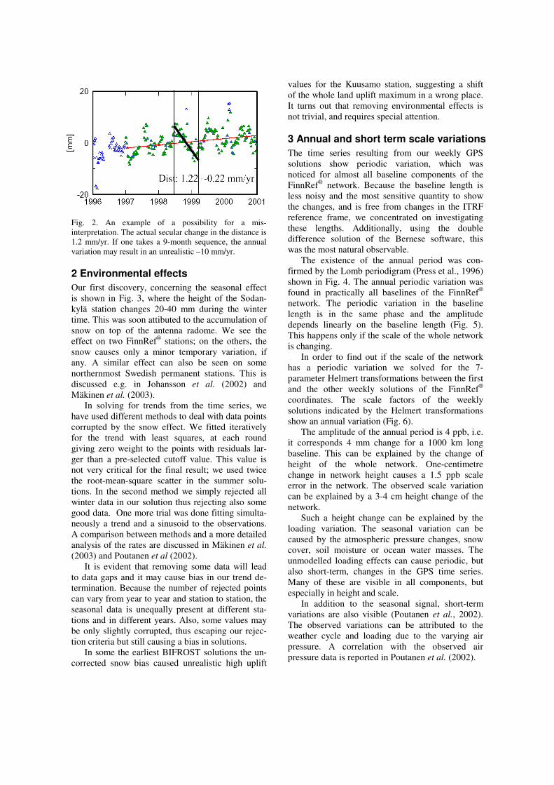
Fig. 2. An example of a possibility for a mis-interpretation. The actual secular change in the distance is 1.2 mm/yr. If one takes a 9-month sequence, the annual variation may result in an unrealistic –10 mm/yr.

2 Environmental effects

Our first discovery, concerning the seasonal effect is shown in Fig. 3, where the height of the Sodan-kylä station changes 20-40 mm during the winter time. This was soon attibuted to the accumulation of snow on top of the antenna radome. We see the effect on two FinnRef® stations; on the others, the snow causes only a minor temporary variation, if any. A similar effect can also be seen on some northernmost Swedish permanent stations. This is discussed e.g. in Johansson et al. (2002) and Mäkinen et al. (2003).

In solving for trends from the time series, we have used different methods to deal with data points corrupted by the snow effect. We fitted iteratively for the trend with least squares, at each round giving zero weight to the points with residuals lar-ger than a pre-selected cutoff value. This value is not very critical for the final result; we used twice the root-mean-square scatter in the summer solu-tions. In the second method we simply rejected all winter data in our solution thus rejecting also some good data. One more trial was done fitting simulta-neously a trend and a sinusoid to the observations. A comparison between methods and a more detailed analysis of the rates are discussed in Mäkinen et al. (2003) and Poutanen et al (2002).

It is evident that removing some data will lead to data gaps and it may cause bias in our trend de-termination. Because the number of rejected points can vary from year to year and station to station, the seasonal data is unequally present at different sta-tions and in different years. Also, some values may be only slightly corrupted, thus escaping our rejec-tion criteria but still causing a bias in solutions.

In some the earliest BIFROST solutions the un-corrected snow bias caused unrealistic high uplift

values for the Kuusamo station, suggesting a shift of the whole land uplift maximum in a wrong place. It turns out that removing environmental effects is not trivial, and requires special attention.

3 Annual and short term scale variations

The time series resulting from our weekly GPS solutions show periodic variation, which was noticed for almost all baseline components of the FinnRef® network. Because the baseline length is less noisy and the most sensitive quantity to show the changes, and is free from changes in the ITRF reference frame, we concentrated on investigating these lengths. Additionally, using the double difference solution of the Bernese software, this was the most natural observable.

The existence of the annual period was con-firmed by the Lomb periodigram (Press et al., 1996) shown in Fig. 4. The annual periodic variation was found in practically all baselines of the FinnRef® network. The periodic variation in the baseline length is in the same phase and the amplitude depends linearly on the baseline length (Fig. 5). This happens only if the scale of the whole network is changing.

In order to find out if the scale of the network has a periodic variation we solved for the 7-parameter Helmert transformations between the first and the other weekly solutions of the FinnRef® coordinates. The scale factors of the weekly solutions indicated by the Helmert transformations show an annual variation (Fig. 6).

The amplitude of the annual period is 4 ppb, i.e. it corresponds 4 mm change for a 1000 km long baseline. This can be explained by the change of height of the whole network. One-centimetre change in network height causes a 1.5 ppb scale error in the network. The observed scale variation can be explained by a 3-4 cm height change of the network.

Such a height change can be explained by the loading variation. The seasonal variation can be caused by the atmospheric pressure changes, snow cover, soil moisture or ocean water masses. The unmodelled loading effects can cause periodic, but also short-term, changes in the GPS time series. Many of these are visible in all components, but especially in height and scale.

In addition to the seasonal signal, short-term variations are also visible (Poutanen et al., 2002). The observed variations can be attributed to the weather cycle and loading due to the varying air pressure. A correlation with the observed air pressure data is reported in Poutanen et al. (2002).

Snow depth and the UP component from GPS at SODA 1996-1999

0

20

40

60

80

100

1201.1

.96

5.2

.96

11.3

.96

15.4

.96

20.5

.96

24.6

.96

29.7

.96

2.9

.96

7.1

0.9

6

11.1

1.9

6

16.1

2.9

6

20.1

.97

24.2

.97

31.3

.97

5.5

.97

9.6

.97

14.7

.97

18.8

.97

22.9

.97

27.1

0.9

7

1.1

2.9

7

5.1

.98

9.2

.98

16.3

.98

20.4

.98

25.5

.98

29.6

.98

3.8

.98

7.9

.98

12.1

0.9

8

16.1

1.9

8

21.1

2.9

8

25.1

.99

1.3

.99

Date

Sn

ow

de

pth

(c

m)

UP

co

mp

on

en

t (c

m)

Fig. 3. An example of the environmental effect. Dots represent the height component of the Sodankylä GPS station. In winter time the height component may change 2-4 cm. The black area shows the depth of the snow. The antenna height error does not fully correlate with snow depth. The reason is that the snow accumulated on top of the antenna falls down when the temperature rises above zero.

Fig. 4. Two examples of GPS time series and their Lomb periodograms, expressed in the time domain. In the upper plot the distance between stations (Metsähovi – Sodankylä) is about twice the distance in the lower plot (Metsähovi – Joensuu). In both cases the annual peak in the Lomb periodogram (left) is statistically significant.

Fig. 5. Scale change in the Finnish permanent GPS network FinnRef®. The amplitude of the annual variation depends on the distance, so the scale change is about 3-4 ppb.

4 Global and regional scale change

The FinnRef® annual scale variation is in the same phase as the variation of the DORIS positioning system results at the Metsähovi observatory (Man-giarotti et al. 2000). In the DORIS time series we have an indication of phase shift between Northern and Southern hemisphere. Global loading of atmo-sphere, snow and other seasonal varying phenom-ena has been suggested as a reason for this, see van Dam et al. (2001).

The IGS GPS time series shows the same effect, both in the radial component and in inter-station distances. In Fig. 7 we give two examples of IGS time series, one in the Northern hemisphere (IRKT in Siberia), and the other one in the Southern hemi-sphere (YAR1 in Australia) where the phases are opposite.

More stations are shown in Fig. 8. Generally, the variations in the Northern hemisphere have their maximum in summer or autumn, whereas for the Southern hemisphere stations the maximum phases occur in the first quarter of the year. The same behaviour can also be seen in the interstation dis-tances.

Fig. 7. Time series of two IGS stations taken from the IGS ppp solution. IRKT is in the Northern hemisphere, YAR1 in the Southern hemisphere. The phase of the annual variation is opposite.

Fig. 8. Amplitude and phase of radial variation of some IGS GPS stations. The direction of the arrow shows the time of the maximum phase and the size of the circle is the amplitude.

We also studied the scale behaviour of the IGS GPS network solution. Because the annual variation is in different phases globally, we see no periodi-city. The scale in the IGS network is quite constant at a global level (Fig. 9, topmost panel). However, in the Fennoscandian area (Fig. 9, middle panel), there is a secular change, as is seen in the FinnRef® data also. This supports our hypothesis that the postglacial rebound is the reason for this secular change.

Fig. 9 shows also one additional problem connected to the use of the ITRF. The scale of the network is not constant, but it has regional deficienceis because of unmodelled vertical crustal motions.

Fig. 6. Annual variation and a secular trend in the FinnRef® network.

Fig. 9. Scale change in the IGS network. Globally the scale change is quite small and there is only a minor trend (top). Three Nordic stations show a trend of about 1.8 ppb/yr (middle). Six North European stations show much smaller trend (bottom). This indicates that the effect of the postglacial rebound in the GPS network scale is visible.

5 Additional observations

In Fig. 10 we show an example of detecting atmo-spheric loading using GPS. There are two phenomena which are not separable in GPS data if no additional information is available. First, the changing air mass and humidity causes a change in the tropospheric path delay, and secondly, the crust is displaced by varying loading. Both phenomena can be in cm-range and thus well within the detection limit of GPS observations.

In connection to the data reduction for the Metsähovi superconducting gravimeter, we have calculated the atmospheric loading from HIRLAM (High Resolution Limited Area Model) air pressure

data and sea loading from tide gauge data. Loading calculations of the Baltic Sea show that 1 m of uniform layer of water corresponds to 31 nm s–2 in gravity and 11 mm in height.

Validity of both calculations has been confirmed by data from the superconducting gravimeter GWR T020 at Metsähovi. The range of air pressure variation at Metsähovi is 100 hPa. The vertical motion due to air pressure is about four times larger than the loading effect due to the Baltic Sea. Simultaneous regression with the air pressure and the Baltic Sea level in Helsinki gives vertical motion –0.35 mm/hPa and –12.4 mm/m (Virtanen, 2002).

Fig. 10. Atmospheric phenomena on GPS observations. Air pressure variations cause a loading effect that can be up to 3-4 cm. Additionally, air mass and humidity changes affect the tropospheric path delay. These are not separable in the GPS observations.

Metsahovi:Barometer:Airpressure (hPa)

Helsinki:Tide gauge:Sea

07-11-01 15-02-02 26-05-02

960

980

1000

1020

-0.5

-0.0

0.5

1.0

-20

-10

0

10

20Metsahovi:GPS:Radial IGS LU Metsahovi:Theory:Vertical

Fig. 11. (Top) Air pressure at Metsähovi [hPa] from September 2001 to July 2002. (Middle) Sea level [m] at the Helsinki tide gauge. (Bottom) IGS radial component [mm] of Metsähovi GPS station (black) and calculated vertical motion due to the loading (gray).

In Fig. 11 we show the air pressure variation at

Metsähovi during one year, and the sea level variation at the Helsinki tide gauge, about 30 km

Low High

Observer

Air mass, humidity

Loading

from the station. The loading computed from this data and the vertical component of the IGS GPS solution show good correlation in general trends, but many details need still further study. Direct comparison with superconducting gravimeter data is yet to be done.

6 Conclusions

We have discussed various scale-related phenomena in GPS time series. It is obvious that the temporal variation degrades our resolution and should be taken into account in high-precision GPS observations.

GPS observations alone do not solve the problem. We need data from other sources, like air pressure and tide gauge observations, to compute the actual loading on site. A superconducting gravi-meter will give an independent constraint to the vertical motion. This concept is compatible with the IGGOS and ECGN proposals to establish multi-instrument reference networks (Ihde, 2003, Rummel et al., 2001). In the Nordic countries a similar proposal for a NGGOS (Nordic Geodetic and Geodynamic Observing System) has been developed (Poutanen et al., 2003).

New applications, like precise point positioning technique or meteorological applications to estimate the tropospheric water vapour content require even sub-cm accuracy in the satellite range measurements. Our examples show that this is not possible if actual loading is not taken into account. Also regional scale variation requires more careful consideration of secular crustal movements when determing the ITRF reference frame in the future.

References

Johansson J.M., J.L. Davis, H.-G. Scherneck, G.A. Milne, M. Vermeer, J.X. Mitrovica, R.A. Bennett, M. Ekman, G. Elgered, P. Elosegui, H. Koivula, M. Poutanen, B.O. Rönnäng, and I.I. Shapiro (2002): Continuous GPS measurements of postglacial adjustment in Fennoscandia, 1. Geodetic results. J.

Geophys. Res. 107, B8. Ihde J. 2003. European Combined Geodetic Network

(ECGN). 1st call for participation. Implementation of the ECGN stations.

Mäkinen J., H. Koivula, M. Poutanen, V. Saaranen (2003): Vertical velocities in Finland from permanent GPS networks and from repeated precise levelling. Journal of Geodynamics, 38, 443-456.

Mangiarotti, S., A. Cazenave, L. Soudarin, J.-F. Cretaux (2000): Annual vertical crustal motions predicted from surface mass redistribution and observed by

space geodesy, J. Geophys. Res., Vol. 106, No. B3, p. 4277-4291.

Milne G.A., J.L. Davis, J.X. Mitrovica, H.-G. Scherneck, J.M. Johansson, M. Vermeer and H. Koivula (2001): Space-Geodetic Constraints on Glacial Isostatic Adjustment in Fennoscandia. Science, Vol. 291, p. 2381-2385.

Ollikainen, M., H. Koivula and M. Poutanen (2000): The Densification of the EUREF Network in Finland. IAG, Section I - Positioning, Commission X - Global and Regional Geodetic Networks, Sub-Commission for Europe (EUREF). Report on the Symposium of the IAG Subcommission for Europe (EUREF) held in Prague, 2-5 June 1999. Veröffentlichungen der

Bayerischen Kommission für die Internationale

Erdmessung der Bayerische Akademie der

Wissenschaften, Astronomisch-Geodätische Arbeiten, Heft Nr. 60. München. p. 114-122.

Poutanen, M., H. Koivula, M. Ollikainen (2002): On the periodicity of GPS time series. International Association of Geodesy Symposia, Vol. 125. Vistas

for Geodesy in the New Millennium. (Eds J. Ádám and K.-P. Schwarz). IAG 2001 Scientific Assembly, Budapest, Hungary, September 2-7, 2001. pp. 388-392. Springer-Verlag Berlin Heidelberg New York.

Poutanen M., H.-P. Plag, H.-G. Scherneck, P. Knudsen, M. Lilje (2003): NGGOS - Nordic Geodetic and Geodynamic Observing System. A paper presented to

the Presisium of the Nordic Geodetic Commision,

May 30, 2003. Press W.H., S.A. Teukolsky, W.T.Vetterling, and B.P.

Flannery (1996): Numerical Recipes in Fortran 77: The art of scientific computing, Second Edition, Cambridge University Press, ISBN 052143064X.

Rummel, R., Drewes, H., and Beutler, G., 2001. Integrated Global Geodetic Observing System (IGGOS): A candidate IAG project, presented at IAG General Assembly, Budapest, 2001.

Scherneck, H.-G., J.M. Johansson, G. Elgered, J.L. Davis, B. Jonsson, G. Hedling, H. Koivula, M. Ollikainen, M. Poutanen, M. Vermeer, J.X. Mitrovica, and G.A. Milne (2002): BIFROST: Observing the Three-Dimensional Deformation of Fennoscandia. In Ice

Sheets, Sea Level and the Dynamic Earth, (Eds. J.X. Mitrovica and B.L.A. Vermeersen). American Geophysical Union, Geodynamics Series, Volume 29, Washington, D.C., p. 69-93.

van Dam T., J. Wahr, P.C.D. Milly, A.B. Shmakin, G. Blewitt, D. Lavallee, and K.M. Larsson (2001): Crustal displacement due to continental water load-ing. Geophysical Research Letters, Vol. 28, No. 4, p. 651-654.

Virtanen, H. (2002): Air pressure and Baltic Sea loading corrections for gravity data at Metsähovi. Proceedings of the XIV General Meeting of the

Nordic Geodetic Commission (Ed. M. Poutanen, H. Suurmäki). Finnish Geodetic Institute, Kirkkonummi.