Embed Size (px)
Citation preview
SCALE-UP OF LATEX REACTORS AND COAGULATORS: A
COMBINED CFD-PBE APPROACH
by
Jordan M. Pohn
A thesis submitted to the Department of Chemical Engineering
In conformity with the requirements for
the Degree of Doctor of Philosophy
Queen‟s University
Kingston, Ontario, Canada
(May, 2012)
Copyright © Jordan M. Pohn, 2012
ii
Abstract
The successful production of a wide range of polymer latex products relies on the ability to
control the rates of particle nucleation, growth and coagulation in order to maintain control over
the particle size distribution (PSD). The development of advanced population balance models
(PBMs) has simplified this task at the laboratory scale, but commercialization remains
challenging as it is difficult to maintain control over the composition (i.e. spatial distributions of
reactant concentration) of larger reactors.
The objective of this thesis is to develop and test a combined Computational Fluid Dynamics
(CFD) -PBM hybrid modeling framework. This hybrid modeling framework can be used to study
the impact of changes in process scale on product quality, as measured by the PSD. The modeling
framework developed herein differs from previously-published frameworks in that it uses
information computed from species tracking simulations to divide the reactor into a series of
interconnected zones, thereby ensuring the reactor is zoned based on a mixing metric.
Subsequently, an emulsion polymerization model is solved on this relatively course grid in order
to determine the time evolution of the PSD. Examination of shear rate profiles generated using
CFD simulation (at varying reactor scales) suggests that, dependent on conditions, mechanically-
induced coagulation cannot be neglected at either the laboratory or the commercial scale.
However, the coagulation models that are formulated to measure the contributions of both types
of coagulation simultaneously are either computationally expensive or inaccurate. For this reason
the decision was made to utilize a DLVO-coagulation model in the framework. The second part
of the thesis focused on modeling the controlled coagulation of high solids content latexes.
POLY3D, a CFD code designed to model the flow of non-Newtonian fluids, was modified to
communicate directly with a multi-compartment PBM. The hybrid framework was shown to be
well-suited for modeling the controlled coagulation of high solid content latexes in the laminar
iii
regime. It was found that changing the size of the reactor affected the latex PSD obtained at the
end of the process. In the third part of the thesis, the framework was adapted to work with Fluent,
a commercial CFD code, in order to investigate the scale-up of a styrene emulsion polymerization
reaction under isothermal conditions. The simulation results indicated that the ability to maintain
good control of the PSD was inversely related to the reactor blend time. While the framework
must be adapted further in order to model a wider range of polymerization processes, the value of
the framework, in obtaining information that would otherwise be unavailable, was demonstrated.
iv
Co-Authorship
This thesis contains material which has been published in a scientific journal as well as material
that is currently being prepared for submission.
Chapter 3: Pohn, J.; Cunningham, M.; McKenna, T. Modeling Orthokinetic Coagulation in a
Stirred Tank. Manuscript in preparation for submission.
Chapter 4: Pohn, J.; Heniche, M.; Fradette, L.; Cunningham, M.; McKenna, T. Development of a
Computational Framework to Model the Scale-up of High Solid Content Polymer Latex
Coagulators. Published in Chemical Engineering & Technology 11 (2010), 1917 – 1930
Chapter 5: Pohn, J.; Cunningham, M.; McKenna, T. Using a Computational Framework to Model
the Scale Up of Polymer Latex Reactors. Manuscript in preparation for submission.

v
Acknowledgements
This thesis represents the culmination of many years of hard work, sprinkled with occasional
moments of intellectual creativity. I owe my success to a large number of people. Without their
contributions, both large and (seemingly) small, this thesis would not have been written.
I must start off by thanking my supervisors, Timothy McKenna and Michael Cunningham. Both
of you were a constant source of intellectual and creative stimulation. I may have tested your
patience occasionally, but you always found the time to provide me with honest feedback and
encouragement. I hope you find this work a worthy culmination of the effort you invested in me.
I must thank my colleagues and office mates in Kingston for all of their intellectual contributions
and the camaraderie they provided. In no particular order: Niels, Jeff, Mary, Nicky, Ula, Eric,
Jonas, Dan, Julien, Raul and countless others.
I was fortunate to spend extended periods of time during my thesis in both Lyon and Montreal.
I‟d like to thank Franck D‟Agosto at C2P2 for the time he spent training me in the lab during my
stay in Lyon. Although this thesis does not have any NMR spectra (I considered throwing one in
gratuitously), the time you spent with me did not go unappreciated. I must express a sincere debt
of gratitude to Louis Fradette, Mourad Heniche and all of my colleagues at URPEI. Thank you
for taking me in during my nine months in Montreal. The thousands of lines of FORTRAN code
that form the foundation of this thesis stand in evidence of your contributions.
To my friends and family, thank you for your loving support and your patience. I‟d like to thank
my parents, Karen and Stephen. Without your encouragement, I would not have made it to the
end of this long journey.
I‟d like to dedicate this thesis in memory of my grandfather, Oscar Markovitz. Each time I
encountered a roadblock during this journey, stories of your legendary work ethic gave me the
strength to surmount all obstacles.
vi
Table of Contents
Abstract ............................................................................................................................................ ii
Co-Authorship ................................................................................................................................ iv
Acknowledgements .......................................................................................................................... v
List of Figures ................................................................................................................................. ix
List of Tables ................................................................................................................................ xiv
Nomenclature ................................................................................................................................. xv
Chapter 1 Introduction ..................................................................................................................... 1
Chapter 2 Literature Review ............................................................................................................ 6
2.1 Polymer Lattices .................................................................................................................... 6
2.1.1 Early History ................................................................................................................... 6
2.1.2 Emulsion Polymerization Fundamentals ........................................................................ 7
2.1.3 Stability of Polymer Latexes ......................................................................................... 10
2.1.4 High Solids Content Latexes......................................................................................... 12
2.2 Modeling Emulsion Polymerization .................................................................................... 17
2.2.1 Overview of Emulsion Polymerization Kinetics........................................................... 17
2.2.2 Modeling the Particle Size Distribution ........................................................................ 21
2.2.3 Modeling Particle Coagulation ..................................................................................... 21
2.2.4 Modeling Latex Viscosity ............................................................................................. 24
2.3 Simulation of Reactor Performance Using Computational Fluid Dynamics ....................... 31
2.3.1 Overview of Computational Fluid Dynamics Simulation ............................................. 31
2.3.2 Grid Generation ............................................................................................................ 33
2.3.3 CFD Solution Methods ................................................................................................. 34
2.4 Mixing .................................................................................................................................. 35
2.4.1 Overview of Mixing ...................................................................................................... 35
2.4.2 Turbulent Mixing .......................................................................................................... 36
2.4.3 Laminar Mixing ............................................................................................................ 37
2.4.4 Quantifying Mixing ...................................................................................................... 39
2.4.5 Model Hybridization ..................................................................................................... 41
Chapter 3 Modeling Orthokinetic Coagulation in a Stirred Tank ................................................ 46
3.1 Introduction .......................................................................................................................... 46
3.2 Overview of Particle Coagulation Modeling ....................................................................... 49
3.3 Outline of CFD Simulation Method..................................................................................... 59
vii
3.4 Results and Discussion ........................................................................................................ 66
3.4.1 CFD Simulation Results ............................................................................................... 66
3.4.2 Comparison of simple shear model vs. rigorous solution to the convection-diffusion
equations ................................................................................................................................ 78
3.5 Conclusions .......................................................................................................................... 87
Chapter 4 Development of a Computational Framework to Model the Scale Up of High Solid
Content Polymer Latex Coagulators .............................................................................................. 88
4.1 Introduction .......................................................................................................................... 88
4.2 Overview of Framework Components ................................................................................. 92
4.2.1 Mixing System .............................................................................................................. 92
4.2.2 The Population Balance ................................................................................................ 93
4.2.3 Coagulation Kernel ....................................................................................................... 96
4.2.4 CFD Model ................................................................................................................. 100
4.2.5 Latex Rheology ........................................................................................................... 102
4.3 Framework Overview ........................................................................................................ 105
4.4 Simulation Conditions ....................................................................................................... 109
4.5 Results & Discussion ......................................................................................................... 111
4.6 Conclusions ........................................................................................................................ 120
Chapter 5 Using a Computational Framework to Model the Scale Up of Polymer Latex Reactors
..................................................................................................................................................... 121
5.1 Introduction ........................................................................................................................ 121
5.2 Simulation Conditions ....................................................................................................... 125
5.2.1 Description of Process ................................................................................................ 125
5.2.2 Description of the Recipes .......................................................................................... 127
5.2.3 Description of the Mixing System .............................................................................. 130
5.3 Framework Components .................................................................................................... 134
5.3.1 Emulsion Polymerization Model ................................................................................ 135
5.3.1.1 Aqueous Phase Kinetics ....................................................................................... 137
5.3.1.2 Surfactant Adsorption .......................................................................................... 145
5.3.1.3 Monomer Balance ................................................................................................ 149
5.3.1.4 Particle Nucleation ............................................................................................... 151
5.3.1.5 Particle Population Balance Model ...................................................................... 152
5.3.1.6 Coagulation Kernel .............................................................................................. 163
5.3.1.7 Latex Rheology .................................................................................................... 165
viii
5.3.2 CFD Model ................................................................................................................. 166
5.3.3 Automatic Zoning Algorithm...................................................................................... 171
5.4 Results & Discussion ......................................................................................................... 176
5.4.1 Blending Simulations & Zone Generation .................................................................. 177
5.4.2 Framework Predictions ............................................................................................... 189
5.5 Conclusion ......................................................................................................................... 206
Chapter 6 Concluding Remarks ................................................................................................... 207
References .................................................................................................................................... 213
ix
List of Figures
Figure 2.1. Simple schematic illustrating the effect of diameter ratio on a bimodal packing
arrangement. .................................................................................................................................. 15
Figure 2.2. A simplified packing model used to determine the coordination number. The hatched
area represents common space that is shared with other hypothetical spheres.63
.......................... 30
Figure 3.1. Schematic of the reactor geometry used in this work and the key design dimensions.60
Figure 3.2. Two-dimensional slice of the computational mesh showing the hexahedral elements
and the grid refinement near the impeller where velocity gradients are expected to be highest. ... 63
Figure 3.3. Vertical cross-sectional slices showing the change in the velocity magnitude profile as
the tank geometry is scaled from 1 L to 10 m3, maintaining a constant volumetric holding power
input (P/V ratio). NI is set to 100 RPM at the 1-L scale, 35.9 RPM at the 100-L scale and 12.9
RPM at the 10-m3 scale. ................................................................................................................. 68
Figure 3.4. Vertical cross-sectional slices showing the evolution in the localized shear rate profile,
computed with Equation (3.4), as the tank geometry is scaled from 1 L to 10 m3, maintaining a
constant volumetric holding power input (P/V ratio). NI is set to 100 RPM at the 1-L scale, 35.9
RPM at the 100-L scale and 12.9 RPM at the 10-m3 scale. ........................................................... 70
Figure 3.5. Vertical cross-sectional slices showing the change in the Peclet number profile as the
reactor is scaled from 1 L to 10 m3, maintaining a constant volumetric holding power input (P/V
ratio). NI is set to 100 RPM at the 1-L scale, 35.9 RPM at the 100-L scale and 12.9 RPM at the
10-m3 scale. .................................................................................................................................... 71
Figure 3.6. Vertical cross-sectional slices showing the variation in the flow profile at both the 1-L
(top) and 10-m3 (bottom) reactor scales when the dynamic viscosity model is set as constant (left)
or modeled with the Careau-Yasuda model (right). NI is set to 100 RPM at the 1-L scale and 12.9
RPM at the 10-m3 scale. ................................................................................................................. 74
Figure 3.7. Vertical cross-sectional slices showing the variation in the particle Peclet number
profile at both the 1-L (top) and 10-m3 (bottom) reactor scales when the dynamic viscosity model
is set as constant (left) or modeled with the Carreau-Yasuda model (right). NI is set to 100 RPM
at the 1-L scale and 12.9 RPM at the 10-m3 scale. ........................................................................ 75
Figure 3.8. Vertical cross-sectional slices showing, for a higher solids content (59 vol.-%), the
differences in the velocity profile (top) and the particle Peclet number profile when the dynamic
viscosity model is changed from a constant approximation (left) to the Carreau-Yasuda (right). NI
is set to 12.9 RPM. ......................................................................................................................... 77
x
Figure 3.9. Normalized rate of aggregation between equal sized colloidal particles in the presence
of an extensional flow field as a function of Pe. T = 298K, r1 = r2 = 25 nm, 𝛆 = 6.91 × 10-
10 s
2C
2m
-1kg
-1, ψ = 50 mV, for varying ionic strength; conditions are identical to those used to
generate Fig. 3a in Lattuada et al.47
). The lines with symbols were generated using Equation
(3.21), accounting for hydrodynamic interactions in the velocity field; the solid lines (no
symbols) were generated using Equation (3.21), assuming a = 1.0; the dashed lines (no symbols)
were generated using Equation (3.24) which does not account for hydrodynamic interaction
effects in the computation of the velocity field. ............................................................................. 81
Figure 3.10. Dependency of the stability ratio on the local particle Peclet number for binary
collisions between equal-sized colloidal particles, as computed using Equations (3.21) and (3.24).
𝛆 = 6.91 × 10⁻¹⁰
s2C
2m
-1kg
-1, T = 298 K, 𝛋 = 3.21×10
8 m
-1 and 𝛙 = 3.35×10
-2 V........................ 84
Figure 3.11. Dependency of the stability ratio on the local shear rate for binary collisions between
equal-sized colloidal particles, as computed using Equations (3.21) and (3.24). 𝛆 = 6.91 × 10-
10 s
2C
2m
-1kg
-1, T = 298 K, 𝛋 = 3.21×10
8 m
-1 and 𝛙 = 3.35×10
-2 V. ............................................. 85
Figure 3.12. Dependency of the stability ratio on the local shear rate for binary collisions between
equal-sized colloidal particles under unstable conditions, as computed using Equations (3.21) and
(3.24). Simulation conditions are based on those used to generate Figure 3.10, except 𝛋 =
1.52×10⁸ m
-1 and 𝛙 = 2.04×10
-2 V. .............................................................................................. 86
Figure 4.1. Computational domain: (a) three-dimensional structure of the vessel including main
features, (b) vertical slice through the z-axis showing details of unstructured mesh. .................. 102
Figure 4.2. Schematic diagram of the framework, outlining the direction(s) of communication
between the different framework components. ............................................................................ 106
Figure 4.3. (a) Rate of flow exchanged in the vertical direction along the height of a 1 L vessel, as
determined from a preliminary CFD flow field. The rate of exchange was rendered dimensionless
using the maximum rate of flow exchange which is located in the vicinity of the impeller. (b) The
tank was divided into five zones, using four horizontal cut-off boundaries (two above the region
of maximum flow exchange and two below). This zoning procedure required two cut-off values
of the dimensionless rate of flow exchange (log[FL/FL,max] = -0.75, -2.0). Note that the bottom-
most zone was very thin compared to the other four zones and hence it is not shown in this
diagram. ....................................................................................................................................... 109
Figure 4.4. Effective maximum packing fraction, as used in Equation (4.30), for monodisperse
latexes with varying (overall) polymer particle volume fraction. ................................................ 112
Figure 4.5. Vertical cross-sectional slices showing the change in flow intensity as the tank
geometry is scaled from 1 L to 100 L. NI is set to 100 RPM at the 1-L scale, 59.9 RPM at the 10-
xi
L scale and 35.9 RPM at the 100-L scale. Flow data is from CFD simulations based on the initial
PSD (dp = 150, PI = 1.10, 59 vol.-% solids) and reactor conditions (T = 298 K, [S] = 9 mol/m3).
..................................................................................................................................................... 115
Figure 4.6. Simulation predictions for a 10 L vessel in which coagulant was continuously fed into
the vessel in the impeller zone. T = 298 K; NI = 59.9 RPM; [S] = 9 mol/m3. At t = 215 s, the
concentration of coagulant was 140 mol/m3. a) Predicted evolution of the particle size distribution
in a 10 L vessel over a period of 215 seconds b) Zone-by-zone breakdown of the PSD at t = 215s.
..................................................................................................................................................... 117
Figure 4.7. Comparing the PSDs obtained at t = 215 s in vessel in which coagulant was
continuously fed into the vessel in the impeller zone. T = 298K; [S] = 9 mol/m3. At t = 215 s, the
concentration of coagulant was 140 mol/m3. NI was set to 100 RPM at the 1-L scale and 59.9 at
the 10-L scale. The “perfectly mixed” vessel represents a reactor where conditions can be
adjusted to ensure that the timescale of mixing is must faster than the timescale of other dynamic
processes (coagulation, polymerization, heat transfer, etc.). ....................................................... 118
Figure 5.1. Schematic illustrating the emulsion polymerization scenarios that were investigated
via the simulation framework. In the first scenario, initiator, surfactant and monomer are fed into
the vessel within a small region at the start of the simulation. The dispersal of the reactants is not
instantaneous; the size of the reactor will affect blend performance which, in turn, will affect the
evolution of the latex PSD during the nucleation phase. In the second scenario, the initiator, the
surfactant and a fraction of the total monomer are premixed during the nucleation phase. The
framework is used to predict the impact of non-instantaneous monomer dispersal during the
particle growth phase. .................................................................................................................. 130
Figure 5.2. Schematic diagram of the framework. Note that the direction of communication is
from the CFD model to the PBM model only. ............................................................................. 135
Figure 5.3. Schematic of the aqueous-phase and phase-transfer events that occur in an emulsion
polymerization process.7 .............................................................................................................. 139
Figure 5.4. Computational grid: (a) Three-dimensional structure of the vessel showing the main
features and the liquid level; this corresponds to the liquid level during the secondary particle
nucleation phase of the emulsion polymerization process (under the simulation conditions
specified). The reactant feed zone, which is also the tracer injection location in the transient
species tracking simulations, is highlighted in red. (b) Two-dimensional slice of the
computational mesh showing the hexahedral elements and the grid refinement near in the
impeller where velocity gradients are expected to be highest. ..................................................... 170
xii
Figure 5.5. Schematic representation of the automatic zoning algorithm used to generate the zone
grid. .............................................................................................................................................. 172
Figure 5.6. Illustration of the layer-by-layer algorithm for automatic zone construction. ........... 174
Figure 5.7. Simulation results showing the effect vessel scale-up on the time evolution of the
normalized tracer concentration variability, as defined by Equation (5.91). Reactor volume is
scaled from 1 L to 10 m3, adjusting the impeller rotational speed to maintain a constant
volumetric power input (P/V ratio). Feed was injected near the liquid surface level. ................. 179
Figure 5.8. Variation in the computed 95% blend time with (i) vessel scale and (ii) scale-up
approach. η ≈ 5.9 × 10⁴ kg/m/s. Note that geometric similarity is always maintained. Maintaining
a constant tblend at 10 m3 would be physically unrealizable due to motor requirements, so this
simulation was not run. ................................................................................................................ 180
Figure 5.9. Vertical cross-sectional slices showing the change in flow intensity (top) and tracer
dispersion performance (bottom) as the tank geometry is scaled from 1 L to 10 m3. The impeller
rotational speed is adjusted with the objective of maintaining a constant volumetric holding
power input (P/V ratio). NI is set to 100 RPM at the 1-L scale, 35.9 RPM at the 100-L scale and
12.9 RPM at the 10-m3 scale. Flow data is from CFD simulations based on the conditions at the
start of the reaction (η ≈ 5.9 × 10⁴
kg/m/s). ................................................................................ 183
Figure 5.10. Vertical cross sectional slices of a vessel at the 100-L scale showing the variation in
the tracer front time distribution with scale-up objective. Flow data is from CFD simulations
based on the conditions at the start of the reaction (η ≈ 5.9 × 10⁴ kg/m/s). ................................ 185
Figure 5.11. Schematic demonstrating the adaptation of the tracer front distribution to generate
the network-of-zones grid for the 1 L vessel. η ≈ 5.9 × 10⁴ kg/m/s; NI = 100 RPM. The large
circular zone is the feed zone. ...................................................................................................... 188
Figure 5.12. Illustrating the effect of changing the vessel height and the tracer injection location
on the layout of the PBM grid generated for a 10 m3 vessel with the LBL automatic zoning
algorithm. η ≈ 5.9 × 10⁴ kg/m/s; NI = 12.9 RPM. ....................................................................... 193
Figure 5.13. Simulation results predicting the PSD of the latex product obtained at the end of a
semi-batch process (t = 1.75 hours. The initial polystyrene latex is a low solids content
monomodal latex comprised of particles with a mean diameter of 150 nm. A second mode of
particles is nucleated via an injection of surfactant and initiator and the two modes are then grown
together over a period of 1.75 hours. Scale-up is performed maintaining constant P/V. Note that
the PSD of the initial latex is included for reference. .................................................................. 196
Figure 5.14. Predicted impact of reactor scale-up on Np using the polymerization conditions
described in Figure 5.13. The initial polystyrene latex is a low solids content monomodal latex
xiii
comprised of particles with a mean diameter of 150 nm. A second mode of particles is nucleated
via an injection of surfactant and initiator and the two modes are then grown together over a
period of 1.75 hours. .................................................................................................................... 198
Figure 5.15. Simulation results predicting the PSD of the latex product obtained at the end of a
semi-batch process (t = 1.75 hours). The initial polystyrene latex is identical to the initial latex
described in Figure 5.13. The surfactant, initiator and an extra 50 wt.-% monomer are pre-
dispersed in the vessel at the start of the simulation to eliminate the effect of reactor
inhomogeneity on the particle nucleation step. Styrene is fed into the reactor over a period of 1.75
hours to growth the two particle modes together. Note that the PSD of the initial latex is included
for reference. ................................................................................................................................ 200
Figure 5.16. Simulation results demonstrating the impact of vessel scale-up criteria on the PSD of
the final latex, varying the scale-up objective. The three simulations run at the 100-L scale were
scaled-up from the 1-L base case scenario by adjusting the impeller rotational speed to meet three
different scale-up objectives. The polymerization conditions are identical those described in
Figure 5.13. The initial polystyrene latex is a low solids content monomodal latex comprised of
particles with a mean diameter of 150 nm. A second mode of particles is nucleated via an
injection of surfactant and initiator and the two modes are then grown together over a period of
1.75 hours. .................................................................................................................................... 202
Figure 5.17. Simulation results demonstrating the impact of vessel scale-up criteria on the PSD of
the final latex. The reactor is scale-up from 1 L to 10 m3 using the constant torque-per-unit-
volume (TQ/V) approach. The polymerization conditions are identical those described in Figure
5.13. The initial polystyrene latex is a low solids content monomodal latex comprised of particles
with a mean diameter of 150 nm. A second mode of particles is nucleated via an injection of
surfactant and initiator and the two modes are then grown together over a period of 1.75 hours.
..................................................................................................................................................... 203
Figure 5.18. Variation in a) the theoretical maximum packing fraction and b) the zero-shear
viscosity of the final product latex with (i) vessel scale and (ii) scale-up approach. Note that
geometric similarity is maintained. The polymerization conditions are the same as those described
briefly in Figure 5.13. The initial polystyrene latex is a low solids content monomodal latex
comprised of particles with a mean diameter of 150 nm. A second mode of particles is nucleated
via an injection of surfactant and initiator and the two modes are then grown together over a
period of 1.75 hours. .................................................................................................................... 205
xiv
List of Tables
Table 3.1. Parameters used to model the solid concentration-dependence of the Carreau-Yasuda
model parameters for a polystyrene latex.5 .................................................................................... 62
Table 3.2. Effect of viscosity model used in CFD simulation on average flow field properties for a
10 m3 reactor filled with a high solid content latex (59 vol.-%). NI was set to 35.9 RPM. ........... 76
Table 5.1. Change in impeller rotational speed as a function of reactor scale and the scale-up
objective. Note that the required adjustment to the impeller rotational speed is computed using
heuristic that assume the systems are geometrically similar and that that flow is fully turbulent.
..................................................................................................................................................... 133
Table 5.2. Aqueous-phase reaction scheme assumed for modeling styrene emulsion
polymerization. ............................................................................................................................ 138
Table 5.3. Kinetic rate coefficient equations for styrene emulsion polymerization as implemented
in the population balance model .................................................................................................. 143
Table 5.4. Miscellaneous model parameters for styrene emulsion polymerization, as implemented
in the population balance model .................................................................................................. 144
Table 5.5. Definition of the terms appearing in Equation (5.59) for the 0-1-MP and the PB
model128
........................................................................................................................................ 158
xv
Nomenclature
a prefactor parameter
( , , )xa f y vector of aggregation terms (part m-3
[x]-1
s-1
)
ˆ( , )ia v v fraction of chains with 1
ˆi iv v v to the ith class
sa minimum area occupied by a surfactant molecule on the particle surface (m2)
A Hamaker constant (J)
sA area occupied by a surfactant molecule on the particle surface (m2)
totA total particle surface area (m2 m
-3)
ˆ( , )ib v v fraction of chains with 1
ˆi iv v v assigned to the ith class
sb Lagmuir adsorption isotherm parameter (m3 mol
-1)
B birth term (part m-3
[x]-1
s-1
)
c particle concentration (m-3
)
bulkc bulk particle concentration (m-3
)
seedc seed cell from CFD mesh
C dimensionless particle concentration
iC finite volume cell with centre of ri
meshC total number of mesh cells
minC minimum number of mesh cells per zone
maxC maximum number of mesh cells per zone
,z mergeC number of cells in a zone z after a merge attempt
CMC critical micelle concentration (mol m-3
)
0
CMC critical micelle concentration in the absence of added ionic species (mol m-3
)
xvi
pd particle diameter (m)
D death term (part m-3
[x]-1
s-1
)
0D mutual diffusion coefficient between particles (m2 s
-1)
D particle number average diameter (m)
iD particle diameter (m)
ID impeller diameter (m)
mpD diffusivity of monomer in particle phase (m2 s
-1)
mwD diffusivity of monomer in aqueous phase (m2 s
-1)
rdD diffusion coefficient of radical chain end resulting from chemical reaction (m2 s
-1)
xD xth moment of the particle size distribution
D diffusion tensor (m2 s
-1)
e charge on a single electron (C)
e vector of terms to be integrated explicitly (part m-3
[x]-1
s-1
)
[ ]E electrolyte concentration (mol m-3
)
iEM aqueous-phase concentration of exit-derived (desorbed) oligomers of
chain length i
,f hydrodynamic interaction potential
( , )z r tf vector number density function in zone z (part m-3
m-1
s-1
)
, ( , )z mf r t number density function for particles containing radicals of type m in
zone z (part m-3
m-1
s-1
)
If initiator efficiency
iF feed rate of species i (kg/s)
xvii
LF rate of flow exchange in the axial direction (m3 s
-1)
,G hydrodynamic interaction function
h flux function
,H hydrodynamic interaction function
( )He x Heaviside function
I intensity of segregation
I ionic strength (mol m3)
,i jI interface between zone i and zone j
iIM aqueous-phase concentration of initiator-derived oligomers of chain length i
critj critical degree of polymerization for homogenenous nucleation –
initiator-derived radicals
Ecritj critical degree of polymerization for homogenenous nucleation –
exit-derived radicals
Bk Boltzmann‟s constant (J K-1
)
dk rate coefficient for initiator decomposition in the aqueous phase (s-1
)
desk rate coefficient for radical desorption from particles (m3 mol
-1 s
-1)
diffk rate coefficient for the contribution of reaction diffusion to the overall
propagation rate coefficient (m3 mol
-1 s
-1)
,
i
e partk entry rate coefficient for i-meric radical into a polymer particle (m3 mol
-1 s
-1)
,
i
e mick entry rate coefficient for i-meric radical into a surfactant micelle (m3 mol
-1 s
-1)
pk particle phase propagation rate coefficient for long chains (m3 mol
-1 s
-1)
xviii
0pk particle phase propagation rate coefficient for monomeric radical (m3 mol
-1 s
-1)
pwk aqueous phase propagation rate coefficient (m3 mol
-1 s
-1)
pwik aqueous phase propagation rate coefficient for i-meric radical (m3 mol
-1 s
-1)
pik particle phase propagation rate coefficient for i-meric radical (m3 mol
-1 s
-1)
tk particle phase termination rate coefficient for long chains (m3 mol
-1 s
-1)
ij
tk particle phase termination rate coefficient between an i-meric radical and j-meric
radical (mol m-3
s-1
)
0tk termination rate coefficient for monomeric species (m3 mol
-1 s
-1)
trk rate coefficient for transfer to monomer (m3 mol
-1 s
-1)
,i j
twk aqueous phase termination rate coefficient between an i-meric radical and a j-
meric radical (mol m-3
s-1
)
,K x y rate coefficient of volumetric growth arising from chain propagation (s-1
)
micK partition coefficient of styrene between the micellar and aqueous phases (mol-1
)
L end-to-end distance between particles (m)
m dimensionality vector
,i jm mass of species i in phase j (kg m-3
)
M number of measurement locations
M number of finite volumes
i
M concentration of monomer in phase I (mol m-3
)
sat
iM concentration of monomer in phase i at saturated conditions (mol m
-3)
mic micelle concentration (mol m-3
)
xix
rMw molar mass of reactant r (kg mol-1
)
n nucleation vector
( , )N x t number density function (part m-3
[x]-1
)
aggn aggregation number of the surfactant
in number of radicals in particle of size i
n average number of radicals per particle
cutoffn number of cutoff boundary values
zonesn number of zones
AN Avogadro‟s number (mol-1
)
cN number of carbon chains on a surfactant molecule that reside at the interior of a
micelle
IN impeller rotational speed (s-1
)
PN total number of particles per unit volume in the system (part m-3
)
rN number of particles containing r radicals (part m-3
)
,z iN number of particles in cell i of zone z (part m-3
)
,
m
z iN number of particles of type m in cell i of zone z (part m-3
)
zN number of zones to be created
,minzN minimum number of zones to be created
,maxzN maximum number of zones to be created
p pressure (Pa)
ijp spin ratio
P power consumed (J s-1
)
xx
Pe particle Peclet number
yzq volumetric flow rate from zone y to zone z (m3 s
-1)
( )zQ i net flow for species i in zone z (m3 s
-1)
r vector of radial growth rates (m s-1
)
ir radius of particle i (m)
ir size of cell i (m)
lr lower crossover radius (m)
micr radius of micelle (m)
nucr radius of nucleated particle (m)
sr swollen radius of particle (m)
ur upper crossover radius (m)
R universal gas constant (J mol-1
K-1
)
R center-to-center distance between particles (m)
R kinetic coupling matrix
micR rate of micellar nucleation (mol m-3
s-1
)
,mic iR rate of micellar nucleation due to type-i oligomeric radicals (mol m-3
s-1
)
homR rate of homogeneous nucleation (mol m-3
s-1
)
hom,iR rate of homogeneous nucleation due to type-i oligomeric radicals (mol m-3
s-1
)
nucR total rate of particle nucleation (mol m-3
s-1
)
piR rate of polymerization in phase i (mol m-3
s-1
)
pR total rate of polymerization (mol m-3
s-1
)
Re Reynolds number
xxi
s dimensionless distance between particle surfaces
( , , )z z Xxs f y source function vector in zone z for model type X (part m-3
[x]-1
s-1
)
s average sphere packing coordination number
[ ]S total surfactant concentration (mol m-3
)
w
S surfactant concentration in the aqueous phase (mol m-3
)
t polymerization time (s)
blendt reactant blend time (s)
frontt tracer time front (s)
T temperature (K)
iT total radical concentration of length i in the aqueous phase (mol m-3
)
giT glass transition temperature of species i (K)
QT torque (kg m2 s
-2)
'u velocity fluctuation in x direction (m s-1
)
v velocity vector (m s-1
)
rv velocity vector in rotating frame (m s-1
)
v particle volume (m3)
v vector of volumetric growth rates (m3 s
-1)
'v velocity fluctuation in y direction (m s-1
)
v̂ unswollen volume of a new particle formed by aggregation (m3)
cv volume of a CFD mesh cell (m3)
convv convective velocity (m s-1
)
iv unswollen volume corresponding to ri (m3)
xxii
intv interaction velocity (m s-1
)
AV attractive potential (V)
iV molar volume of species i (m3/mol)
intV DLVO interaction potential (V)
intV dimensionless DLVO interaction potential
fV free volume inside particle system
,f satV free volume inside particle system when fully-saturated with styrene monomer
fiV free volume of pure species i
minV minimum volume of a stable particle (m3)
RV reactor volume (m3)
RV DLVO repulsive potential (V)
wV volume of aqueous/water phase (m3)
zV total volume of zone z (m3)
'w velocity fluctutation in z direction
ijW Fuchs‟ stability ratio
,A mx fraction of component A at measurement location m
Ax average fraction of component A in a binary mixture
ix number fraction of size i
AX number of additional solubilized monomeric molecules per micelle
zy continuous phase vector in zone z
z counter-ion valence
xxiii
feedz feed zone
iz zone i
critz critical degree of polymerization for entry
Greek Letters
fast coagulation rate coefficient between particles i and j in the absence of particle
interaction (m3 part
-1 s
-1)
ij coagulation rate coefficient between particles i and j (m3 part
-1 s
-1)
shear rate (s-1
)
th characteristic shear thickening time (s)
Stern layer thickness (m)
hydrodynamic interaction boundary layer thickness (m)
,i j Delta Kronecker function
merge homogeneity of merged zones
tracer time front homogeneity (s)
rate of turbulent energy dissipation (m2 s
3)
permittivity of water (s2 C
2 m
-1 kg
-1)
0 vacuum permittivity (s2 C
2 m
-1 kg
-1)
r relative permittivity of water
( )r hybrid population balance model smoothing function
fluid viscosity (kg m-1
s-1
)
0 fluid viscosity at zero shear (kg m-1
s-1
)
xxiv
fluid viscosity at infinite shear (kg m
-1 s
-1)
s viscosity of aqueous medium (kg m-1
s-1
)
intrinsic viscosity
inverse Debye length (m-1
)
dimensionless particle size ratio
t turbulent viscosity (kg m-1
s-1
)
density of continuous phase (kg m-3
)
E rate coefficient of entry of desorption-derived radicals into a latex particle (s-1
)
I rate coefficient of entry of initiator-derived radicals into a latex particle (s-1
)
i density of pure species i (kg m-3
)
T rate coefficient of entry of all radicals into a latex particle (s-1
)
particle surface charge density (C m-2
)
particle interaction coefficient
r radius of interaction of reactants (m)
t turbulent Schmidt number
characteristic shear thinning time (s)
stress tensor (Pa)
kinematic viscosity (m2 s
-1)
potential correction factor (V)
dimensionless particle center-to-center distance
volume fraction of particles
eff effective volume fraction of particles
xxv
i volume fraction of species i inside a particle
m effective maximum packing fraction
,m hs maximum packing fraction for monodisperse hard spheres
,m i effective maximum packing fraction for monodisperse particles of diameter Di
ult ultimate packing fraction
time-dependent scalar
des rate of radical desorption from particles (mol m-3
s-1
)
particle surface potential (V)
Ω angular velocity vector (rad s-1
)
zeta potential (V)
1
Chapter 1
Introduction
Polymer latexes, colloidally-stable dispersions of nanoscale polymer particles dispersed in a
continuous medium, are a commercially-important class of materials. Polymer latexes are used in
a wide range of applications not limited to interior and exterior surface coatings, paper finishing,
adhesives, carpet backing and bulk polymer production.1 The typical polymer latex recipe is
comprised of monomer, water, stabilizer (surfactant), initiator and buffer and most polymer
latexes products are produced via emulsion polymerization, although further processing steps
(such are particle coagulation) are often required.2 Early polymer latex formulations and
production strategies were often a product of trial and error, perhaps with the aid of an early
kinetic model.3 Today that is no longer the case, as scientists and engineers have a much better
grasp on the underlying phenomena that govern the manufacturing process.4 By carefully
manipulating the nucleation, growth and coagulation of polymer particles during all stages of
manufacture, the properties of the final latex can be tailored to meet an ever-growing range of
applications.
For economic reasons, it is becoming ever more important to increase the solids content in
industrial recipes, which requires careful manipulation of the particle size distribution (PSD) at all
stages of production.5, 6
With the assistance of state-of-the-art emulsion polymerization models,
i.e. those constructed using a population balance model (PBM) framework,7, 8
researchers have
developed new manufacturing strategies that offer improved control over the particle size
distribution.9 Commercialization of these manufacturing strategies, however, remains a great
2
challenge because it becomes increasingly difficult to maintain control over reactor composition
as the size of the reactor is increased.
Originally, process scale-up strategies were developed using heuristic techniques,10
and tested via
extensive pilot plant experimentation. Today, industry has widely-adopted the use of
computational fluid dynamics (CFD) simulation11
in the scale-up process. CFD simulation, first
widely-used in the field of aerodynamics,12
can predict fluid flow inside stirred tanks, often
providing information that is difficult to obtain or unavailable experimentally.13
CFD simulation
is currently used to predict the impact of reactor scale-up on blending time14
and to identify other
mixing problems that may arise13
(e.g. regions of excessively high shear rates, poor heat transfer).
In the production of polymer latexes, the impact of poor mixing on the time evolution of latex
PSD can, in theory, be modeled by combining CFD simulation with an appropriate process
model. However, the population balance equations that comprise the most advanced polymer
latex process models cannot presently be incorporated directly in the CFD code (or vice versa)
due to memory restrictions.
These restrictions can be overcome through the clever use of hybrid modeling, where the
population balance equations are solved on coarser grid of zonal compartments, which is
generated using flow information obtained via CFD simulation. Alexopoulos and Kiparissides15,
16 and Elgebrandt et al.
15, 16 have used CFD simulation to investigate mixing inside emulsion
polymerization reactors, identifying regions of high shear where coagulum is more likely to form.
These groups subsequently developed hybrid multizonal/CFD models that used the information
computed from CFD simulation to study the evolution of latex PSDs under conditions of
3
inhomogeneous shear. The models were restricted to studying low concentration latexes and the
process kinetics were simplified considerably.16
The objective of the present work is to develop a combined CFD-PBM modeling framework that
incorporates a detailed emulsion polymerization population balance model. The framework is
used to investigate the impact of changes in key process length and time scales on the properties
of latex products. This was accomplished by developing a set of numerical codes in FORTRAN
which were designed to model the nucleation, growth and coagulation of polymer latex particles
under different process conditions and interface with different CFD simulation codes. Special
attention was paid to the efficiency of the algorithms used within the framework, in order to
ensure that the framework could be run on a modern desktop (or laptop) computer, making the
approach accessible to a wide audience.
This work represents the first known attempt to develop a hybrid CFD-PBM framework
specifically for the purposes of modeling reactor scale-up. With regards to modeling emulsion
polymerization, the framework presented in this thesis represents advancement on the previously-
published emulsion polymerization hybrid CFD-PBM models found in the literature.15, 17
First,
the model presented in this work is capable of the polymerization and coagulation of polymer
latexes over a wider range of conditions (e.g. low and high solids contents). Second, the
generation of the network-of-zones (the grid on which the PBM is solved) can be generated
automatically using data from transient species blending simulations.
4
The remainder of the thesis is comprised as follows:
Chapter 2 is a bibliographic review and overview covering emulsion polymerization,
computational fluid dynamics and fluid mixing.
Chapter 3 deals with the modeling of shear-induced coagulation, as this mechanism is
typically neglected in the formulation of emulsion polymerization PBMs.7 CFD
simulation is used to investigate the changes in the distribution of shear forces within in a
reactor as the process is scaled-up to assess the importance of shear-induced coagulation
at both the laboratory and commercial scales. Even under conditions where shear-induced
coagulation is known to be important, modeling particle coagulation in flow conditions
where both electrostatic and shear-induced forces interact with each other remains a
challenge. To begin addressing this challenge, the modeling predictions of a
computationally-efficient coagulation kernel are compared to a recently-developed
coagulation model that offers improved predictive capabilities in order to determine if the
computationally-efficient kernel could be incorporated into a PBM.
Chapter 4 discusses, in detail, the construction of a hybrid CFD-population balance
model framework. The framework was developed specifically to study non-Newtonian
latexes and the POLY3D CFD simulation code was extensively modified in order to
function within the framework environment. The hybrid multizonal/CFD framework was
used to investigate the effect of vessel scale on the deliberate coagulation of a high solids
content latex.
Chapter 5 builds on the framework developed in the previous chapter. An advanced
automatic zoning procedure was developed in order to zone the reactor using the results
of species tracking simulations, which is an original approach not employed in
5
previously-published hybrid modeling frameworks. The hybrid multizonal/CFD
framework is used to investigate the impact of reactor scale-up on the production of a
polystyrene latex produced via emulsion polymerization.
Chapter 6 is a summary of the thesis‟ main conclusions and a list of recommended
directions for future study.
6
Chapter 2
Literature Review
2.1 Polymer Lattices
2.1.1 Early History
The production of synthetic polymer latexes, as a means of developing an alternative to natural
rubber, began shortly following the conclusion of World War I with the development of the
emulsion polymerization (EP) process technique. Rubber occurs in nature as latex, so the hope
was that the mechanical properties of synthetic rubbers would be improved if they were produced
under conditions in which the final product resembled the natural product, at least in appearance.
In addition to improved product properties, emulsion polymerization was found to sport a number
of additional advantages over bulk and solution polymerization, mainly higher rates of
productivity and controllability. The outbreak of World War II led to a world-wide natural rubber
shortage, which motivated the United States government to form a synthetic rubber program that
brought rubber-manufacturing and oil companies together in a cooperative effort. While the main
objective of this program was to guarantee a supply of rubber for the war effort, the extensive
amount of research carried out by industry and academia during World War II established
emulsion polymerization and polymer latex technology as active fields of research following the
end of the war. Much of our understanding of the underlying mechanisms of emulsion
polymerization is a result of the fundamental research carried out by Harkins,18
Smith and Ewart.3
In the years following the end of World War II, researchers extended the range of products and
applications that made use of emulsion polymerization technology. Today, a wide range of
synthetic latexes, with rubbery and non-rubbery polymers, are produced using emulsion
polymerization. Beyond the production of bulk polymer, the range of applications includes1
1
paints, coatings (including paper finishing), adhesives and carpet backing, with annual
production exceeding 20 million tonnes.{{38 de la Cal, J.C. 2005}}
7
2.1.2 Emulsion Polymerization Fundamentals
A typical industrial emulsion polymerization recipe contains monomer, water, surfactant, initiator
and additives, such as buffers and chain transfer agents. Commercial scale emulsion
polymerization is typically carried out in large stirred tank vessels operating in semi-continuous
mode, although batch and continuous processes are also used. The monomer is dispersed in water
along with surfactants (typically anionic or nonionic or a combination of both), forming
emulsified monomer droplets (~ 1 – 10 μm in diameter).19 The surfactant will partition between
the surface of the droplets and the aqueous phase. If the surfactant concentration exceeds the
critical micelle concentration (CMC), the point at which the surfactant completely covers the
monomer droplets and saturates the aqueous phase, micelles will form. The interior of the
micelles is hydrophobic and hence the micelles will swell with monomer. Additionally, a small
fraction of the total monomer in the system will partition into the aqueous phase, the amount
being dependent on monomer solubility. Polymerization is usually initiated using a water soluble
initiator, although oil-soluble initiators may be used.{{38 de la Cal, J.C. 2005}} In terms of the
decomposition mechanism, thermal initiators (such as potassium persulphate) are the most
common type of initiator employed. Redox initiators, such as hydrogen peroxide / ascorbic acid,
may be employed when the polymerization is carried out at a lower temperature.20
The original EP reaction theory proposed by Harkins sought to divide the EP process into three
intervals. While the interval model is applicable to ab-initio (non-seeded) batch emulsion
polymerization only, the interval theory approach still serves as a helpful starting point for
understanding a wider range of EP processes. Interval I is the particle nucleation stage, Interval II
8
is the particle growth stage, while Interval III is marked by the consumption of remaining
monomer in the droplets.
The primary radicals derived from initiator decomposition react with the monomer dissolved in
the aqueous phase, adding monomer units. Once a sufficient number of monomer units have been
added, the oligomer becomes surface active and is capable of entering the monomer-swollen
micelles (if present) to form precursor particles. This is known as micellar or heterogeneous
nucleation. The length of the critical length chain length at which the oligomer becomes surface
active is dependent on the water solubility of the monomer, increasing with water solubility; for
reference, styrene becomes surface active after two chain units have been added. Entry into
micelles is statistically favoured over entry into the monomer droplets because total surface area
of the droplets (~ 105 m
2 / m
3) is relatively small in comparison to the total surface area of the
micelles (~ 108 m
2/m
3 ).
19 Surface active oligomers will continue to grow in the aqueous phase, if
they are not captured by a micelle or another particle. However, when an aqueous phase oligomer
reaches a critical chain length, it will become water insoluble and undergo a coil-to-globule
transition, excluding water and becoming a precursor particle.21
This mechanism is known as
homogeneous nucleation. The critical chain length is, like the surface active chain length, directly
proportional to the water solubility of the monomer; for styrene, the critical chain length is around
five added monomer units. Homogeneous nucleation is dominant when operating below the
CMC, as micelles are not present. When operating slightly below the CMC, local micelles may
form due to inhomogeneous distribution of the surfactant. Above the CMC, heterogeneous
(micellar) nucleation is the dominant mechanism, although homogeneous nucleation still
occurs.22
Micelles that have not been nucleated will dissociate to stabilize the growing particles.
9
Once the micelles have been depleted, new particles will not form through heterogeneous
nucleation, although the micelle population may be renewed when particles coagulate and the
total particle surface area is reduced. In systems dominated by homogeneous nucleation, particle
formation may continue to occur throughout the course of polymerization, but the precursor
particles may quickly coagulate in the absence of free surfactant and will essentially reach a
steady-state value.21
The timescale of monomer diffusion is rapid compared to the rate of
polymerization inside the particles. As an example, for styrene EP at 50 ℃, the rate at which
monomer molecules are consumed per particle is approximately 1.4 × 10⁴ s
-1, while the
maximum rate at which monomer molecules can replenished per particle is in the order of
1.0 × 10⁹ s
-1 (see Gilbert,
4 page 52 for a details). When the maximum rate of monomer
replenishment is many orders of magnitude higher than the rate of monomer consumption, the
monomer droplets act as monomer stores, keeping the monomer concentration inside particles
nearly constant (this is not always the case; see Zubitur et al.23
for a discussion of diffusional
limitations).
Once the monomer droplets have been completely depleted the remaining monomer in the
particles is exhausted. The onset of the gel effect,24
a decrease in the bimolecular termination rate
due to the viscous environment inside the particles, may lead to an increased rate of
polymerization, more-than-offsetting the decrease in monomer concentration inside the particles.
Polymerization is ideally carried out as close to 100% conversion as possible, although a limiting
conversion may be encountered if the glass transition temperature of the polymer is higher than
the reaction temperature. In many end-use applications residual monomer poses a health hazard,
10
necessitating its removal via stripping, which adds a significant expense to the manufacturing
process.
Emulsion polymerization has inherent advantages over solution and bulk polymerization. The use
of water as the dispersion medium (as opposed to volatile organic solvents) leads to a reduced
environmental impact and low product odor, and effectively functions as a heat sink during
polymerization. The viscosity of the product latexes is reduced compared to bulk and solution
polymerization processes, allowing for easier handling operation, especially in the case of
rubbery and/or film forming materials. The maximum attainable conversion is higher, so
emulsion polymerization products contain lower volatile organic compounds (VOCs) compared
to products produced using solution or bulk polymerization. Furthermore, under certain
conditions, the radicals in emulsion polymerization are compartmentalized and cannot terminate
with radicals existing within another particle. This can lead to higher polymerization rates and
higher average molecular weights than what would be achievable using bulk or solution
polymerization.
2.1.3 Stability of Polymer Latexes
Polymer latexes are thermodynamically unstable. The intermolecular forces of attraction cause
molecules in the condensed state to cohere together.2 Thus, there is a thermodynamic tendency
for the polymer particles to coagulate together, eventually resulting in complete phase separation.
The aggregation and coalescence of polymer particles reduces the total interfacial area between
the particle and the aqueous phases, thereby reducing the total Gibbs free energy of the system.
The mechanism by which aggregation and coalescence occurs is the Brownian motion of the
11
particles, although velocity gradients in the flow field at the microscopic scale (on the order of
particle diameter) may enhance the motion of particles relative to one another. While most
polymer latexes are thermodynamically unstable, they are kinetically stable; that is, the rate at
which the system proceeds towards thermodynamic equilibrium is sufficiently retarded such that
it is not uncommon for a polymer latex product to have a shelf life measured in years. The source
of this kinetic stability is the presence of a potential energy barrier which discourages particles
from approaching one another closely. The barrier arises from a balance between attractive and
repulsive forces; as a general rule, the higher the potential energy barrier, the more stable the
latex.
The forces of attraction acting between particles in a polymer solution are collectively known van
Der Waals forces, which arise from electric dipoles in the atoms. The electric dipoles may be
permanent, induced by other molecules or simply a result of fluctuations in the atoms‟ electron
clouds. The magnitude of the van Der Waals forces depends on the composition and shape of the
polymer particles and the composition of the medium in which they are dispersed.2 The forces of
repulsion which act between particles can be grouped into four types: (i) electrostatic forces,
which depend on the presence of an electric charge at the surface of the particles; (ii) steric
forces, which arise from the presence of hydrophilic molecules bound to the surface of the
particles; (iii) depletion forces, which arise from the presence of hydrophilic macromolecules
dissolved in the aqueous phase; (iv) solvation forces, which arise from the binding of molecules
of the dispersion medium to the surface of the particles. Researchers have developed quantitative
models for electrostatic and steric stabilization, but the stability conferred through the depletion
and solvation forces is difficult to quantify. In particular, depletion stabilization is difficult to
12
differentiate from steric stabilization due to the tendency of hydrophilic molecules that are
dissolved in the aqueous media to adsorb on the surface of the particles.2
2.1.4 High Solids Content Latexes
Natural rubber latex, when it flows out from the tree, is only ~30 wt.% polymer, the remainder
being mostly water.2 One of the key developments that led to the commercial exploitation of
natural rubber in the earlier 20th century was the discovery of industrially-feasible methods
whereby natural rubber latexes could be concentrated to ~60 wt.% polymer without
compromising the stability of the latex. For both natural and synthetic polymer latexes, solids
concentration is often a key consideration when developing and manufacturing commercially
exploitable latexes for two reasons: (i) the production and transport of concentrated latexes is
more economical, an especially-important consideration for manufacturers of commodity-grade
latexes; (ii) high solid content latexes are uniquely-suited to a wide range of applications (for
example, fast-drying paints and coatings). For many synthetic latexes, however, there is a
practical loading limit, typically around 55 vol.-%, above which the latex becomes difficult to
process due to a sharp increase in latex viscosity and less colloidally-stable as a result of the
increasing frequency of particle collisions.25
This upper loading limit is strongly dependent on the
particle size distribution (PSD) and the nature of the stabilizing layer (surfactant). One advantage
inherent to synthetic polymer latexes is the ability to control the PSD of the latex product by
manipulating the manufacturing process. Recently published results suggest that it is possible to
prepare low viscosity, stable latexes with solid loading above 70 vol.-% if the PSD is well-
engineered.26, 27
13
Hard (non-deformable) spheres can pack in a variety of ways, ranging from simple cubic
(SC; m 0.52 ) to face-centered cubic (FCC;
m 0.74 ), amongst other packing
arrangements. At m
the particles are unable to move past one another, corresponding to
infinite viscosity. It has been demonstrated experimentally and computationally that if the hard
spheres are introduced into a control volume and gently shaken they will pack randomly; some of
the spheres will arrange themselves in a SC scheme and others will take on the FCC packing
arrangement; the resulting arrangement is referred to as random close packing (RCP; m 0.64
).28
At high shear limits, however, the energy imparted by the mean flow will cause the particles
to align in a denser random packing structure (m 0.71 );
5, 29 these aligned structures are also
responsible for the shear thinning.
The stabilization layer surrounding the latex particle is deformable under shear, so latexes are not
considered hard spheres; rather they behave as soft (deformable) spheres.30
Due to this extra
layer, the effective volume faction (eff ), is greater than the volume fraction of the solid particles
alone ( ):
3
1 seff
s
t
r
(2.1)
where st is the thickness of the stabilizing layer. For particles that are stabilized with non-ionic
surfactant, st is a function of the volume fraction and the shear rate , although at high shear
rates st is influenced by volume fraction only.
5 When ionic stabilization is present,
1
st , the
Debye length. The Debye length quantifies the thickness of the counter-ion layer that surrounds
the charged particle surface and is typically on the order of 10-9
m to 10-8
m thick. When
14
describing the packing limits of soft sphere systems, it is important to note that the packing limits
are based on the effective volume fraction (eff ), thus the maximum packing fraction of soft
sphere systems is always less than the maximum packing fraction of hard sphere systems.
Equation (2.1) states that a stabilizer layer of a given thickness will have a greater impact on the
effective packing fraction of a system of small particles compared to a system of large particles,
as it takes up a relatively higher volume fraction for small particles than for large ones. For a
given fraction of surfactant and ionic strength, all things being equal, the maximum packing
fraction of latex particles increases as the particle size increases.
Bimodal and multimodal packing arrangements, with smaller particles filling the interstices that
exist in the large particle lattice, offer the potential for increased packing density (a higher
maximum packing fraction) compared to monodisperse latexes with narrow PSDs. This is not
always the case however. The maximum packing fraction is determined by the thickness of the
stabilizer layer and the PSD. Schneider et al. demonstrated that a poorly adjusted PSD for a
bimodal system (i.e. too many very small particles or “fines”) may have a lower maximum
packing fraction than a monomodal PSD.31
The maximum packing fraction is highest when there
are just enough small particles to fill all of the interstices of the large particle lattice; research has
shown this occurs when volume fraction ratio of large to small particles is around 4 – 5.32
The
size ratio between the large and small particles is just as important as the volume fraction ratio.
The small particles must be small enough to fit inside the interstices within the large particle
lattice, however if the small particles are too small, multiple occupancy of the interstices may
actually push the large particle lattice apart,28
as illustrated schematically in Figure 1. According
to experiments performed by Greenwood et al., the optimal diameter ratio ( /l sd d ) between the
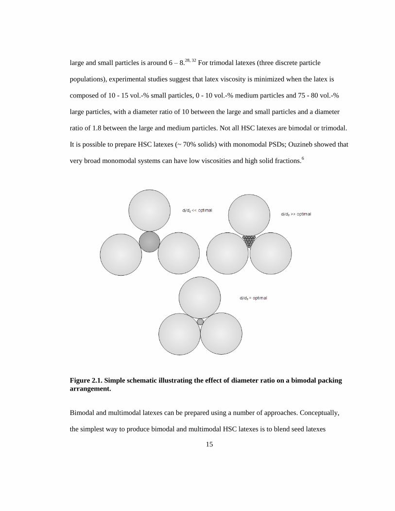
15
large and small particles is around 6 – 8.28, 32
For trimodal latexes (three discrete particle
populations), experimental studies suggest that latex viscosity is minimized when the latex is
composed of 10 - 15 vol.-% small particles, 0 - 10 vol.-% medium particles and 75 - 80 vol.-%
large particles, with a diameter ratio of 10 between the large and small particles and a diameter
ratio of 1.8 between the large and medium particles. Not all HSC latexes are bimodal or trimodal.
It is possible to prepare HSC latexes (~ 70% solids) with monomodal PSDs; Ouzineb showed that
very broad monomodal systems can have low viscosities and high solid fractions.6
Figure 2.1. Simple schematic illustrating the effect of diameter ratio on a bimodal packing
arrangement.
Bimodal and multimodal latexes can be prepared using a number of approaches. Conceptually,
the simplest way to produce bimodal and multimodal HSC latexes is to blend seed latexes
16
together and concentrate them through evaporation under vacuum, an energy-intensive operation.
Schneider et al.33
utilized this approach to prepare concentrated pressure sensitive adhesives (78%
BA, 19.5% MMA, 2.5% AA) with trimodal PSDs. While conceptually simple, the blending and
evaporation approach is unfeasible for commercial production. Concentrated latexes can also be
prepared through the growth of multi-modal seed populations in semi-continuous operation. It is
extremely difficult to obtain a solid content above 50% with a batch configuration due to
uncontrollable homogeneous nucleation (controlling the PSD is key obtaining high solids, as
discussed above). In semi-continuous operation the surfactant concentration can be controlled,
ensuring the free surfactant concentration remains low enough to maintain control over the
formation of new particle. Homogeneous nucleation is essentially unavoidable in the presence of
water soluble monomer however the feed rates and types of initiator and surfactant can be
adjusted to control whether or not these particles are stabilized. A variation on this approach is to
create a large particle seed via ab initio emulsion polymerization (semi-continuous operation)
then create secondary and tertiary populations through in situ nucleation, typically accomplished
with a shot of surfactant and monomer. Once all of the particle populations are present, large and
small particle alike are grown simultaneously through the continuous addition of monomer (and
surfactant) until the desired solid content and PSD are obtained. Ceteris peribus, the smaller
particles will grow faster, as their higher total surface area leads to preferential radical capture.
This approach is popular in industry since it is outwardly the simplest process with the fewest
processing and handling steps.30
Due to the high commercial interest in concentrated multimodal
latexes, much of the early research is found in patents rather than the open literature. For an
overview of the patents in this field, refer to the review by Guyot et al.30
or Schneider et al.34
Recently there have been some notable studies published in the open literature. Schneider et al.
17
produced a four-part study of HSC latexes in emulsion that included investigations into the
synthesis of primary particle seeds35
and concentrated lattices34
and the role of oil-soluble
initiators in maximizing solids content and latex robustness.33
Together these papers provide a
framework for producing concentrated latexes (> 70 wt.-% polymer) with reasonably low
viscosities (between 0.3 and 1.0 Pa-s at a shear rate of 20 s
-1). Boutti et al.
9, 36, 37 proposed a
procedure that can be used to synthesize low viscosity (less than 1.5 Pa-s at a shear rate of 20 s-1
)
bimodal BA/MMA/MAA latexes with very high solid contents over 70 wt.-% without the use of
seed particles, such that the entire process is carried out in a single reactor. Ai et al.27
prepared
poly(MMA/BA/AA)/poly(styrene/AA) composite latexes with a solid content of 70 wt.-% and
demonstrated that the two-phase structure of the corresponding latex film led to the formation of
an integral film at room temperature that sported an improved mechanical strength over the non-
composite poly(MMA/BA/AA) latex film.
2.2 Modeling Emulsion Polymerization
2.2.1 Overview of Emulsion Polymerization Kinetics
The polymerization in emulsion systems follows the same basic mechanisms as in bulk
polymerization, with the key difference being compartmentalization; that is, radicals existing in
one particle cannot terminate with the radicals located in other particles. In bulk and solution
polymerization, the rate of polymerization (per unit volume of aqueous phase) is normally
defined as the rate of consumption of monomer:
[ ][ ]p p
d MR k M R
dt (2.2)
18
where pk
is the propagation rate coefficient, M is the concentration of monomer and R is
the total radical concentration. In emulsion polymerization (most cases) nearly all polymerization
occurs in the particle phase so [ ]M is replaced with [ ]pM and the total radical concentration is
/p AnN N , where is the n average number of radicals per particle, pN is the total particle
concentration per unit volume of aqueous phase (e.g. m-3
) and AN
is Avogadro‟s number. When
modeling emulsion processes that require more than one monomer, the rate expression must be
modified. For an example, refer to the modified rate expression based upon the Mayo-Lewis
terminal model,38
which is available in the literature.1
Smith and Ewart3 developed a set of differential equations to track the number of particles
containing r free radicals (rN ) based on the adsorption of radicals from the aqueous phase,
desorption of free radicals into the aqueous and termination of free radicals within the particles.
The population of the latex particles is normalized such that 0
1r
r
N
and the average number
of radicals per particle is given by 1
r
r
n rN
. A population balance takes on the following
form:
1 1
2
1
2 1 1
r
r r T r r des
r r t
dNN N r N rN k
dt
r r N r r N k
(2.3)
Where T is the average rate of entry of free radicals into the particles, desk is the rate
coefficient of desorption of free radicals out of the particles and tk is the relative rate coefficient
19
for termination inside the particles. These rate coefficients are dependent on a number of
variables including I (initiator concentration), pN ,
pd (particle diameter), and n itself. At
pseudo steady-state ( / 0rdN dt ), Smith and Ewart found that there were three limiting cases:
Case 1: 0.5n (fast desorption; T desk )
Case 2: 0.5n (no desorption and fast termination; des T tk k )
Case 3: 0.5n (fast absorption relative to termination; T tk )
Equation (2.3) and the Smith-Ewart limiting cases are valid only under the assumption that
radical loss by termination can be expressed using a single rate coefficient, tk (i.e. the rate
coefficient is independent of chain length). It is currently accepted however that the termination
coefficient depends on the degrees of polymerization of the two terminating chains.39
Therefore
Equation (2.3) must not only track the number of particles with radicals per particle r, but also the
number of particles 1,2,3,...,
r
nN with a degree of polymerization of 1,2,...,n. The pseudo-first-order
rate coefficient will strongly depend on 1,2,3,...,
r
nN , making Equation (2.3) invalid. However
almost every emulsion polymerization system can be categorized as approximately fitting one of
two simplifying limits: „zero-one‟ and „pseudo-bulk‟.21
A „zero-one‟ system is one in which the entry of a radical into a particle already containing a
growing chain results in „instantaneous‟ termination (the timescale of termination is much more
rapid than any other event such as propagation or radical desorption); this model does not require
a termination coefficient expression. The „zero-one‟ limiting version of the Smith-Ewart
equations only allows particles to contain zero or one radical at any point in time, reducing
20
Equation (2.3) to a system of two differential equations. In the case of hydrophobic monomers
such as styrene, particles containing one radical are further divided into two types: those
containing a single unit radical derived from the transfer-to-monomer reaction (radical desorption
is allowed) and those containing one oligomeric or polymeric radical (radicals with chain lengths
greater than a single unit are sufficiently hydrophobic that they do not exit the particle), resulting
in a system of three differential equations. Two further limit approximations to the „zero-one‟
model exist: complete aqueous phase termination whereby all desorbed radicals are terminated in
the aqueous phase, and complete re-entry whereby all desorbed radicals re-enter another latex
particle. The latter limit (with the additional assumption that the monomeric radicals are far more
likely to propagate at least once before exiting a second time) is said to govern most styrene
emulsion polymerizations.
The other widely-applicable limit is the „pseudo-bulk‟ limit in which the compartmentalization of
radicals into particles has no effect on the system kinetics. The „pseudo-bulk‟ limit is valid when
desorbed free radicals never terminate in the aqueous phase (jumping from particle to particle
until eventually propagating) and/or the value of n is sufficiently high ( 0.7n ) that intra-
particle kinetics are the same as in a bulk system. For monomers with sufficiently high
propagation rate coefficients, n can be less than 0.5 and the particles will still obey „pseudo-
bulk‟ kinetics because the rate of termination is diffusion-controlled40
and the chains propagate to
long lengths very quickly upon entering (or re-entering) a particle. Detailed treatment of the
„zero-one‟ and „pseudo-bulk‟ kinetic systems, along with the accompanying time-dependent
expressions ( /dn dt ) are available in Thickett and Gilbert‟s published overview of emulsion
polymerization kinetics.21
21
2.2.2 Modeling the Particle Size Distribution
The particle size distribution is one of the most important characteristics of a polymer latex with
respect to determining its mechanical properties. Careful control over the particle size distribution
in the reactor is especially important in the production of HSC latexes, where the dynamics of
particle nucleation, growth and coagulation have a large impact on the rate of polymerization and
final product properties. The modeling of the rheological properties of the latex depends on
knowledge of the PSD. A means of tracking changes to the particle size distribution during the
course of polymerization is necessary when modeling emulsion polymerization processes that are
sensitive to changes in the PSD. Modeling the evolution of the particle size distribution is
accomplished through the addition of a set of population balance equations (PBEs) to the kinetic
model. For a review on the use and limitations of PBEs in modeling emulsion polymerization, the
reader is referred to the comprehensive review written by Vale and McKenna.8 The formulation
of the PBEs, as they are applied within the framework, is covered in Chapters 4 and 5.
2.2.3 Modeling Particle Coagulation
For modeling purposes, the coagulation between particles is assumed to occur as a result of
binary collision events, although the assumption that all particles will coagulate through a binary
collision mechanism is valid only when working with dilute systems. However, due to the
complexity of formulating and solving the equations for multi-body collisions (never-mind
experimental validation of the parameters), binary collision models have been used at all latex
concentrations.7 There are two mechanisms that govern coagulation in emulsion polymerization:
perikinetic aggregation and orthokinetic aggregation. Perikinetic aggregation results from the
Brownian motion of particles (diffusive forces), while orthokinetic aggregation is facilitated by
22
the motion of the fluid (convective forces). Many researchers neglect orthokinetic aggregation
when modeling emulsion polymerization, as perikinetic aggregation thought to be the dominant
mechanism at small particle sizes (~ 50 nm).41
This simplification is often justified based on
experimental results,42, 43
however theoretical studies of particle coagulation suggest that
hydrodynamics can play an important role when ionic strength is low and the double layer is
thick.44
In relatively stable dispersions there is a strong non-linear coupling between convection
and diffusion which means that the overall coagulation rate coefficient is not equal to the sum of
the two aggregation mechanisms. Until recently, this necessitated the use of empirical expressions
(such as the one employed by Lowry et al.45, 46
) when studying systems where both mechanisms
were thought to contribute, as the semi-phenomenological models were unable to capture the
changing nature of the interaction between the two mechanisms over a full range of shear rates.
As will be discussed extensively in Chapter 3, this is no longer strictly the case.47
In addition to
perikinetic and orthokinetic aggregation, experimental evidence provided by Heller et al. suggests
that surface coagulation may contribute to the overall rate of particle coagulation in
mechanically-agitated systems when flow at or near the interface is fully-turbulent.48-52
The
surface coagulation mechanism appears to be related to the partial deweting of particles at the
interface, either as a consequence of desorption of the stabilizer or heterogeneity of the particle
surface (e.g. a non-spherical shape or parts of the surface are devoid of stabilizer).2 It has been
proposed that particles adsorb at the aqueous phase – air interface where aggregation occurs
between pairs of particles (i.e. binary coagulation). The aggregates then desorb from the surface,
returning to the disperse phase of the latex. Therefore, surface coagulation is typically modeled
under the assumption that adsorption of the particles at the aqueous phase – air interface obeys
the Langmuir adsorption isotherm equation and the rate of aggregation at the surface is second-
23
order. Surface coagulation is not considered in the framework developed in this thesis in order to
simplify matters, but this assumption should be removed when modeling systems where
significant foaming occurs at the surface of the latex.
Perikinetic aggregation is often modeled using the DLVO approach, in which it is postulated that
the coagulation rate coefficient is dependent on the stability of the particles. Particle stability is,
in turn, dependent on the total particle potential energy of interaction, intV . As stated prior, the
total potential energy of interaction is the net sum of all attractive and repulsive contributions,
including van der Waals‟ attraction and electrostatic, steric, depletion and solvation-based
repulsion. The reader may refer to Ottewill53
for details on calculating each of these contributions
and the overall perikinetic aggregation rate coefficient. While the DLVO framework is widely-
used in modeling emulsion polymerization coagulation, the theory has limitations. DLVO-based
models do not provide accurate predictions of the aggregation rates of colloids when the potential
barrier is located at surface distances below 1 – 2 nm and non-DLVO forces dependent on the
structure of the solution and particle surface become important. Additionally, DLVO theory
assumes dilute dispersions in which the influence of surrounding particles on a pair of interacting
particles can be neglected. In concentrated systems (e.g. HSC latexes), the surrounding particles
cause an effective reduction inintV , leading to a lower stability ratio. The concentration effect may
lead to a higher rate of coagulation that would be predicted by DLVO theory. For a complete
overview of the failings of DLVO theory, as applicable to emulsion polymerization, refer to Vale
and McKenna‟s review of PBEs in emulsion polymerization.8 In the development of DLVO-
based models it is assumed that every particle in the system has the same surfactant coverage,
while in reality the precursor particles formed from homogeneous nucleation may undergo
24
coagulation rapidly, such that the surfactant does not have sufficient time to diffuse to the newly-
created surface and equilibrate. Despite this, DLVO theory remains the only basis for non-
empirical modeling available for particle coagulation and it is possible to fit certain model
parameters to obtain coagulation rate coefficients that correctly predict experimental results.
2.2.4 Modeling Latex Viscosity
In the absence of shear thickening, latex viscosity, when plotted as a function of shear rate, can
demonstrate two plateaus. At low shear rates, latex viscosity is independent of shear rate and is
said to obey Newtonian behaviour. This lower plateau is referred to as the lower Newtonian
viscosity. This plateau is readily observed at low to moderate solid concentrations, but does not
appear at very high solid contents.5 At a certain shear rate (characteristic of the latex), the shear
stress transmitted through the aqueous medium will begin orienting the particles in the direction
of flow. These layered particles offer less resistance to flow, hence a lowering of the viscosity.
Once the particles are completely layered, viscosity can no longer decrease with increasing shear
rate and this upper plateau is referred to as the upper Newtonian viscosity. If shear rate is
increased further, the mean flow may impart enough energy to the particles so that they overcome
the forces of repulsion and begin clustering together. This clustering (not to be confused with
coagulation) will disrupt the layered flow which results in a large increase in latex viscosity. This
clustering phenomenon, known as shear thickening, may also result in coagulation which will
exacerbate the increase in viscosity. Shear thickening, if not anticipated, can result in damaged
equipment.54
During the operation of an emulsion polymerization reactor, care must be taken to
ensure the maximum shear rate inside the reactor does not approach the thickening limit.
25
There are a number of equations available for modeling the viscosity of monodisperse
dispersions. Dilute suspensions can be modeled using the Einstein equation:55, 56
1s (2.4)
where s is the viscosity of the continuous medium and is the intrinsic viscosity, a
dimensionless measure of the particles‟ contribution to the suspension viscosity; for hard spheres
2.5 . Equation (2.4) is valid for dilute suspensions (non-interacting particles) only. More
concentrated solutions can be tacked under the assumption that the effect of all particles in a
concentrated suspension is the sum of the effects of particles added sequentially. Under this
assumption, the Einstein equation can be written in differential form as:
d d (2.5)
When a particle is added to a relatively concentrated solution it will require more space than its
volume due to packing difficulties, such that an increase in volume fraction will result in the
particles already present to suffer a „crowding effect‟ which amplifies the increase to viscosity.
Sudduth57
proposed that this crowding effect could be captured by replacing d with
/ 1d k
where is the particle interaction coefficient (an adjustable parameter) and
accounts for the „crowding factor‟. The term 1 k
can be thought of as the relative amount
of unhindered volume that can effect a change in suspension viscosity. The relative amount of
unhindered volume is equal to zero when the maximum packing fraction has been reached.
Numerically: 1 0k
if m , therefore 1/ mk . When modeling latexes, recall that
and m are the effective volume fraction and effective maximum volume fraction, respectively
26
and will vary significantly with particle size due to the presence of the stabilizing layer. Equation
(2.4) can be rewritten as follows:
1 / m
dd
(2.6)
When 1 integration of Equation (2.6) yields the Krieger-Dougherty58
equation:
1
m
s
m
(2.7)
The Krieger-Dougherty equation has been shown to fit the data from a variety of polymer latex
systems, provided accurate a priori estimates of and m are available. Equation (2.7) is very
sensitive to changes in and
m . Therefore when modeling new formulations it is
recommended that new estimations of and m are obtained.
30 Note that setting to 2 and
integrating Equation (2.6) will result in the Mooney equation,59
and fractional values of can
be used when optimizing the empirical fit of data.
The Carreau-Yasuda model has been shown to best capture the shearing behaviour of
concentrated latexes, including the lower and upper Newtonian plateaus and the onset of shear
thinning.5
0
1 / for
1thm a
a
(2.8)
where a and m are adjustable parameters, 0 and
are the zero and infinite shear viscosities,
the shear rate acting upon the latex , is the characteristic time for the onset of shear thinning
and th is the shear rate above which shear thickening occurs. The four parameters vary with the
27
solid content of the lattice; the concentration-dependence for all four parameters can be modeled
with the general form of the Krieger-Dougherty equation:58
,
0
,
1 , , , 1/
m
s th
m
(2.9)
where s is the value of the parameter at zero solids content.
Modeling the viscosity-loading profiles of multimodal latexes requires an estimation of the
maximum packing fraction parameter (m ). While the optimal PSD can often be determined
through extensive experimentation, it is often beneficial to augment experimental efforts with a
well-chosen model. Researchers have developed models that are capable of predictingm for
multi-modal dispersions, provided the related monodisperse maximum packing fraction (0
m ) is
known. Sudduth57, 60
proposed the following model to determine the maximum packing fraction of
a polydisperse system:
5 11 /0 D D
m ult ult m e
(2.10)
Where 5D and
1D are the 5th and 1
st moments of the PSD, is an adjustable parameter and
ult
is the ultimate packing fraction which is calculated as follows:
01 1n
ult m (2.11)
Here, n is the number of discrete particle sizes in the population. For bimodal latex where
particles are arranged according to RCP (this would correspond to a latex under low shear)
0 0.64m , 2n and 0.87ult .28
The xth
moment of the PSD is defined as:
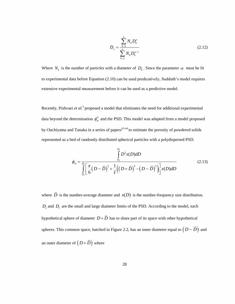
28
1
1
1
nx
k k
kx n
x
k k
k
N D
D
N D
(2.12)
Where kN is the number of particles with a diameter of
kD . Since the parameter must be fit
to experimental data before Equation (2.10) can be used predicatively, Sudduth‟s model requires
extensive experimental measurement before it can be used as a predictive model.
Recently, Pishvaei et al.5 proposed a model that eliminates the need for additional experimental
data beyond the determination 0
m and the PSD. This model was adapted from a model proposed
by Ouchiyama and Tanaka in a series of papers61-64
to estimate the porosity of powdered solids
represented as a bed of randomly distributed spherical particles with a polydispersed PSD.
3
3 3 3
( )
1( )
6
l
s
l
s
D
D
m D
D
D x D dD
D D D D D D x D dDs
(2.13)
where D is the number-average diameter and ( )x D is the number-frequency size distribution.
sD and lD are the small and large diameter limits of the PSD. According to the model, each
hypothetical sphere of diameter D D has to share part of its space with other hypothetical
spheres. This common space, hatched in Figure 2.2, has an inner diameter equal to D D and
an outer diameter of D D where
29
0 for D D
for D D
D D
D D
(2.14)
The average number of spheres sharing the common space is calculated with the following
formula:
2
33
31 ( )
841 8 1
13( )
l
s
l
s
D
Do
m D
D
DD D x D dD
D Ds D
D D D x D dD
(2.15)
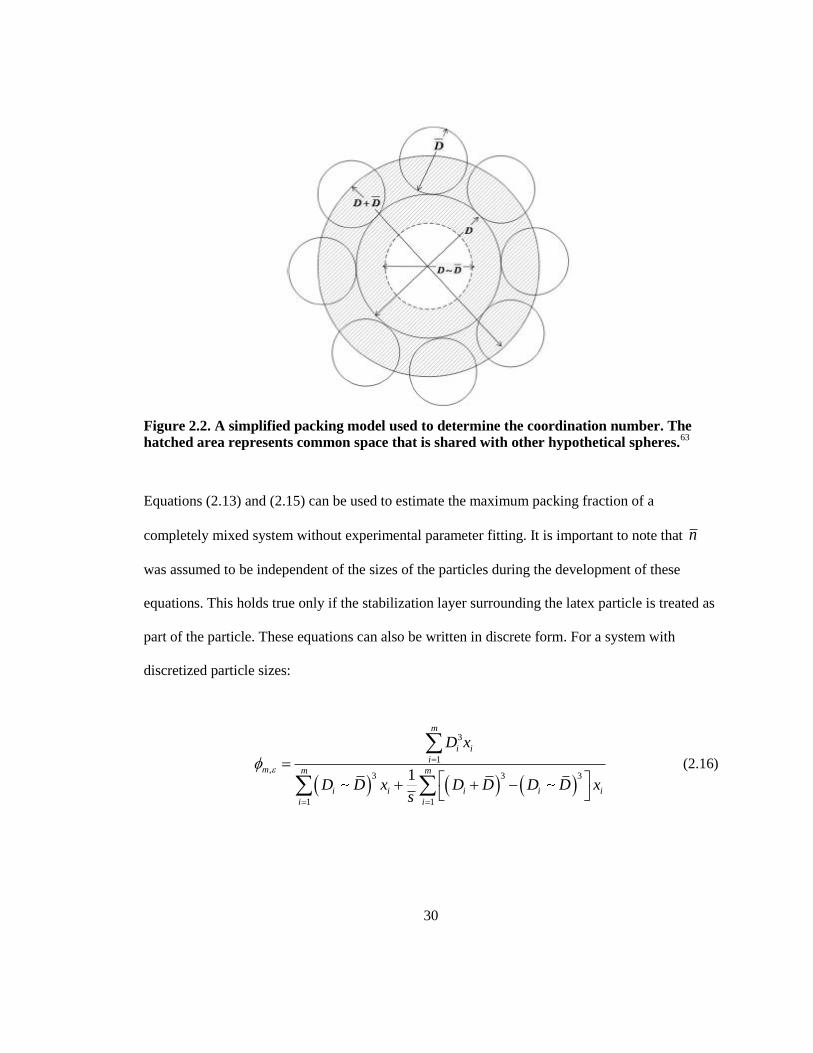
30
Figure 2.2. A simplified packing model used to determine the coordination number. The
hatched area represents common space that is shared with other hypothetical spheres.63
Equations (2.13) and (2.15) can be used to estimate the maximum packing fraction of a
completely mixed system without experimental parameter fitting. It is important to note that n
was assumed to be independent of the sizes of the particles during the development of these
equations. This holds true only if the stabilization layer surrounding the latex particle is treated as
part of the particle. These equations can also be written in discrete form. For a system with
discretized particle sizes:
3
1,
3 3 3
1 1
1
m
i i
im m m
i i i i i
i i
D x
D D x D D D D xs
(2.16)
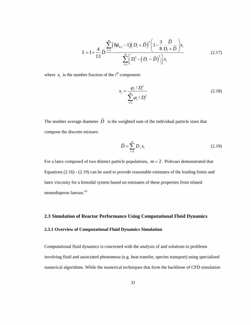
31
2
,
1
33
1
38 1 1
841
13
m
m i i i
i i
m
i i i
i
DD D x
D Ds D
D D D x
(2.17)
where ix is the number fraction of the i
th component:
3
3
1
/
/
i ii m
i i
i
Dx
D
(2.18)
The number average diameter D is the weighted sum of the individual particle sizes that
compose the discrete mixture:
1
m
i i
i
D D x
(2.19)
For a latex composed of two distinct particle populations, 2m . Pishvaei demonstrated that
Equations (2.16) - (2.19) can be used to provide reasonable estimates of the loading limits and
latex viscosity for a bimodal system based on estimates of these properties from related
monodisperse latexes.65
2.3 Simulation of Reactor Performance Using Computational Fluid Dynamics
2.3.1 Overview of Computational Fluid Dynamics Simulation
Computational fluid dynamics is concerned with the analysis of and solutions to problems
involving fluid and associated phenomena (e.g. heat transfer, species transport) using specialized
numerical algorithms. While the numerical techniques that form the backbone of CFD simulation
32
can trace their roots back almost one hundred years, the techniques were not put into practice
until the 1960s, coinciding with the availability of sufficient computing power. The first industry
to make extensive use of CFD was the aerospace industry, which integrated CFD techniques into
the development and manufacture of aircraft and jet engines. The emergence of more affordable
computing power has allowed CFD simulation to fulfill its promise as a complementary addition
to experimental analysis, contributing extensively to both our scientific understanding and
industrial productivity. Today, CFD is used extensively in the field of chemical engineering to
study a wide range of phenomena not limited to: heat transfer, polymeric fluid flow, combustion
analysis and separation and mixing.11
A typical CFD code consists of three elements: (i) the preprocessor; (ii) the numerical solver; and
(iii) the postprocessor. Preprocessing consists of defining the computational domain of interest,
division of the domain into a number of non-overlapping subdivisions (the computational grid)
and the specification of the problem. Specifying the problem includes the selection of
phenomena, definition of the pertinent fluid properties and specification of boundary and initial
conditions. Numerical solvers can be divided into classes, depending on the numerical solution
techniques they employ: finite difference, finite volume, finite element and spectral techniques
(an extension of finite element). Each method has its perceived strengths and weaknesses,
although extensive research developments within each method‟s respective research community
have addressed many of these weaknesses. For example, Sukumar developed a finite difference
technique capable of solving the Poisson equation on unstructured grids.66
Once a solution has
been computed, a post-processor is used to display the domain geometry and grid, view the
solution field, produce graphics and animation and export data. Exported data may undergo
33
further processing in external software or be used as input in an external process model, allowing
for the development of hybrid model frameworks.
2.3.2 Grid Generation
Grid generation strategies can be classified as Cartesian, structured, unstructured, hybrid and
gridless.67
In Cartesian gridding, a network of uniformly-spaced grid lines is placed in a rectangle
(2-D) or rectangular box (3-D). Boundary conditions are implemented by cutting grid lines into
the interior cells. While Cartesian gridding is the simplest way to discretize a given field, the
approach is generally not suited for solving complex computational fluid flow problems. In
structured gridding, the grid is a network of curvilinear coordinate lines such that one-to-one
mapping can be established between physical and computational space.67
The structured grid
approach is the most accurate way to specify boundary conditions as the curvilinear grid points
conform to the shape of the surface/boundary. The main drawback to structured grid generation is
that the method is not automated. Should a user wish to generate a structured grid on a complex
geometry the user must typically divide the structure into simple sub-regions manually before a
set of structured subgrids can be generated. While the process of grid subdivision requires
substantial manual input, structured grids are often computationally efficient, requiring fewer
cells to compute the solution to a desired level of accuracy. Unstructured meshes composed of
either triangles (in 2-D) or tetrahedrons (in 3-D); the grid information is recorded as a set of node
coordinates and a connectivity list, where the neighbor set for each node is specified.
Unstructured meshes are typically generated using automatic algorithms, with the user merely
specifying the desired grid density and (if necessary) the desired increase in mesh density at the
boundaries. The drawbacks of unstructured grids are the higher number of elements required
34
relative to structured grids and the propensity of the automatic generation software to generate
poor quality elements (skewed) in regions with high aspect ratios. The skewed cells may
potentially introduce errors in the numerical solution. Hybrid grids are a méritage of structured
and unstructured meshing, where structured sub-grids are generated in areas that require high
aspect ratio cells and the remainder of the domain is filled with an unstructured mesh. This
approach is capable of generating high quality meshes with a large degree of automation, but the
algorithms are often temperamental and may require the user to be experienced with the pre-
processing software before they function properly. Gridless methods allow for the numerical
treatment of the conservation equations without requiring the use of a mesh topology. The only
structure required is a distribution of cloudless points within the computational domain. Gridless
methods are still a nascent field of research, but the approach holds much promise in modeling
the unsteady motions of rigid bodies, where mesh quality would tend to degrade during large
rigid movements of a body‟s boundaries.12
2.3.3 CFD Solution Methods
CFD software differs from most other modeling software in that most modeling software is
designed to produce solutions for any arbitrary set of user-defined equations, while CFD software
is tailored to obtain the best solution to very specific set of problems; that of fluid flow. Most
commercial CFD packages are well-suited to solving the conservation equations for mass,
momentum, heat and energy; should the need arise to simultaneously solve additional processes
in parallel (for example, a particle population balance), the code is unlikely to be effective.
The most commonly-encountered discretization techniques in both research and commercial code
are the finite element method and the finite volume method. Both methods begin with the integral
35
form of the conservation equation. The finite element method uses simple piecewise functions
(linear or quadratic) to describe variations in the unknown flow variables. The piecewise
functions are substituted into the exact conservation equations and the residuals of the resulting
approximation are minimized by multiplying them by a set of weighing functions and integrating.
The resulting algebraic system of equations is solved to yield the unknown coefficients of the
piecewise approximating functions.68
In the finite volume method, the conservation equations are
integrated over all control volumes of the domain, and the resulting integral expressions are
discretized to form a system of algebraic equations, which are solved using an iterative method.
Both the finite element and finite volume methods are capable of solving fluid flow problems.
Originally, the finite volume method was preferred for its relative conceptual simplicity; the finite
element method is more abstract in concept, but the element construct was well-suited to
unstructured meshes. Over the years, advances in research have addressed both methods‟
weaknesses. For process engineers, the choice of software is likely to be strongly-influenced by
software compatibility and the availability of both technical support and application-specific
support in the research community.
2.4 Mixing
2.4.1 Overview of Mixing
Mixing can be defined as the reduction in inhomogeneity to achieve a desired process result.
When one refers to inhomogeneity, they are typically referring to concentration, phase or
temperature. The failure to achieve good mixing upon process scale-up can lead to myriad
problems, most of which will, ultimately, compromise the commercial viability of the product in
36
question. Mixing is typically said to occur at three scales: (i) macromixing, which is driven by the
largest scales of motion in the fluid and takes place at the scale of the vessel; (ii) mesomixing,
which is the scale reduction stage where inertial and/or viscous forces play an important role
(depending on the flow regime); (iii) micromixing, where molecular diffusivity controls the rate
in reduction in segregation. The mechanisms by which mixing occur will be dependent on the
flow regime; laminar mixing is mechanistically different from turbulent mixing. Beginning with
Danckwerts in the 1950s,69
researchers have developed numerous definitions to quantify the
degree of segregation or inhomogeneity within reactors in order to provide a non-trivial answer to
the question: “How well-mixed is the process?” What follows is a brief summary of the
differences between turbulent and laminar mixing and an overview of how mixing may be
quantified.
2.4.2 Turbulent Mixing
At high Reynolds numbers, flows are observed to become chaotic or turbulent. Turbulent flow is
characterized by a random state of motion in which the velocity and pressure change continuously
with time over substantial regions of flow.11
Visualization of turbulence would reveal the
presence of rotational flow structures called eddies or vortices. The largest eddies acquire energy
through interaction with the mean flow and they, in turn, interact with smaller eddies, transferring
energy to them before breaking-up. These smaller eddies transfer their energy to even smaller
eddies. This so-called energy cascade continues until the eddies are small enough such that their
kinetic energy can be effectively dissipated through viscous action. The energy cascade converts
kinetic energy from the mean flow into heat energy at the molecular level. For demonstrative
purposes, the eddies are typically divided into three sizes. The largest eddies are integral scale
37
eddies, which are highly anisotropic in structure and have a length scale on the order of the mean
flow. The intermediate eddies, the Taylor microscale eddies, are unaffected by the viscous forces,
but can be described by the rate of energy dissipation. The smallest scale eddies are the
Kolmogorov eddies, which are the isotropic in structure and represent the smallest scale at which
segregation (mixing) occurs through the mechanism of turbulence. Turbulence motion enhances
the rate of mixing by breaking up fluid motion, thereby reducing the scale of segregation. In
simplified terms, bulk mixing and turbulence mixing are responsible for reducing the length scale
at which molecular diffusion must act.70
Due to the highly-complex physics of turbulence and the
potential for interactions between the turbulence field and process kinetics, it is often essential to
simplify the modeling of the turbulence field and use scaling arguments to develop relationships
between aggregate turbulent quantities (e.g. the rate of dissipation of turbulent energy) and
important process dynamics (e.g. the maximum rate of fluid shear in a stirred tank). For further
details with regards to turbulence modeling, the reader is referred to Chapter 3 in Versteeg and
Malalasekera.11
For an overview on the role of turbulence in mixing applications, refer to Chapter
3 in the Handbook of Industrial Mixing.70
2.4.3 Laminar Mixing
Mixing applications that are carried out at low velocities or involve high viscosity substances will
be characterized by a laminar flow environment. While the modeling of the physics of fluid flow
is rendered less complex by the absence of turbulence, the quantification of laminar mixing is still
a relatively fresh area of research. Laminar mixing is, from a physical perspective, often more
challenging than turbulent mixing due to the absence of eddies to promote mixing at the meso-
scale. Early researchers, such as Mohr,71
observed that the blending of polymers visually
38
consisted of drawing out separated components into progressively thinner striations and
developed an expression to compute the rate of reduction in striation thickness as a function of
shear rate. However it wasn‟t until the 1980s that researchers developed a general framework for
quantifying the degree and rate of laminar mixing. Aref72
proposed the extension of dynamic
systems theory to study mixing at scales smaller than the scale of bulk fluid flow. Laminar
mixing requires the presence of periodic unsteady fluctuations in the velocity field, generating
chaotic motion. As fluid elements travel through chaotic flow, they are stretched and folded due
to changes in the direction of the flow field acting upon the element. Repetitive exposure to the
stretching and folding cycle (reorientation) results in a reduction in striation thickness and an
increase in contact area between striations. This mechanism is important in mixing processes
because the rate of diffusion of material at the microscopic scale is dependent on the length scale
of striation thickness and the total interfacial area available for transport. The ability to measure
the spatial distribution of striation thickness using the framework of chaotic flow modeling fills in
the gap between macro-mixing and micromixing.73
It has been found that the metrics that have
used successfully to quantify turbulent mixing, such as the coefficient of variance (explained in
the next section), are sometimes unable to predict differences in performance of different laminar
mixers.74
There are a number of approaches available for modeling the distribution and evolution
of striation thickness in laminar flows, such as computing the stretching field, computing striation
thickness distributions directly or predicting them from stretching.73
In CFD simulation,
Lagrangian particle tracking is sometimes employed in place of scalar tracking when modeling
the development of striation thickness to avoid numerical diffusion that is inherent to scalar
tracking.
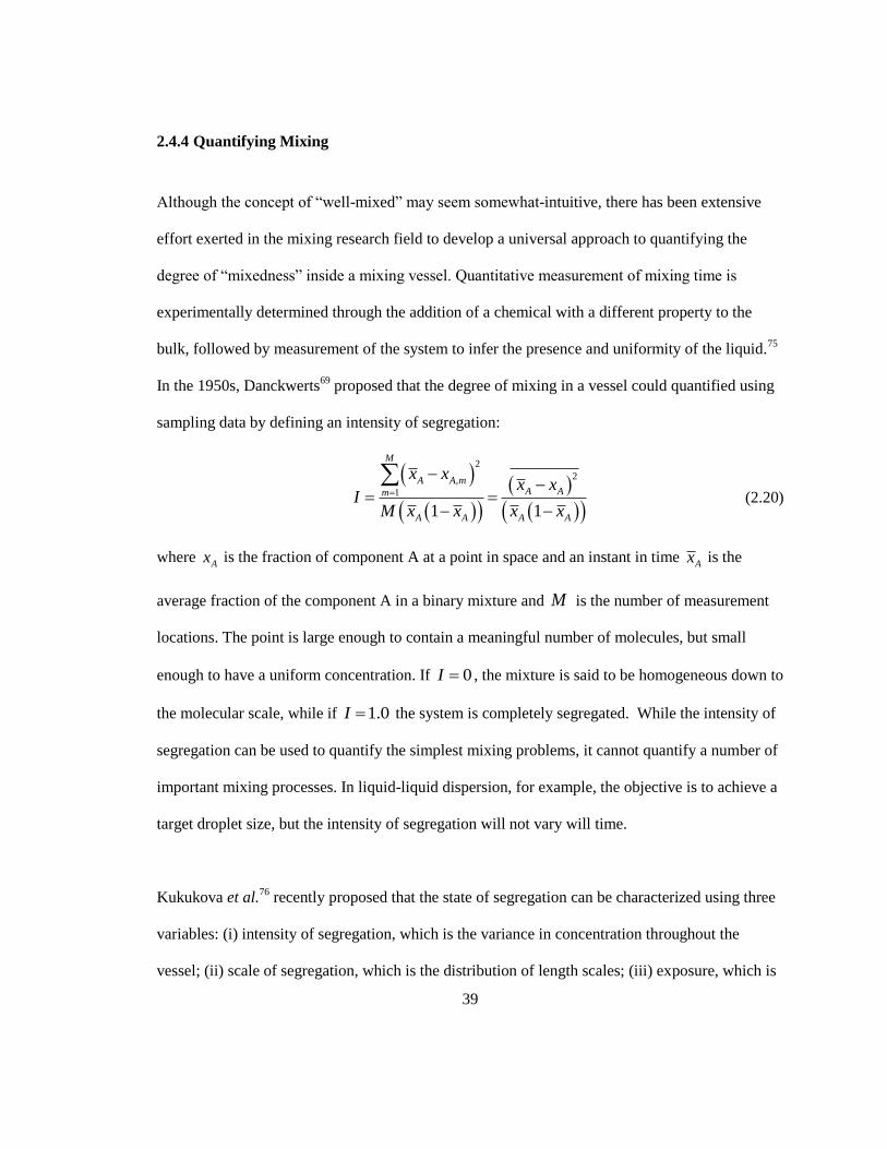
39
2.4.4 Quantifying Mixing
Although the concept of “well-mixed” may seem somewhat-intuitive, there has been extensive
effort exerted in the mixing research field to develop a universal approach to quantifying the
degree of “mixedness” inside a mixing vessel. Quantitative measurement of mixing time is
experimentally determined through the addition of a chemical with a different property to the
bulk, followed by measurement of the system to infer the presence and uniformity of the liquid.75
In the 1950s, Danckwerts69
proposed that the degree of mixing in a vessel could quantified using
sampling data by defining an intensity of segregation:
2
2,
1
1 1
M
A A mA Am
A A A A
x xx x
IM x x x x
(2.20)
where Ax is the fraction of component A at a point in space and an instant in time
Ax is the
average fraction of the component A in a binary mixture and M is the number of measurement
locations. The point is large enough to contain a meaningful number of molecules, but small
enough to have a uniform concentration. If 0I , the mixture is said to be homogeneous down to
the molecular scale, while if 1.0I the system is completely segregated. While the intensity of
segregation can be used to quantify the simplest mixing problems, it cannot quantify a number of
important mixing processes. In liquid-liquid dispersion, for example, the objective is to achieve a
target droplet size, but the intensity of segregation will not vary will time.
Kukukova et al.76
recently proposed that the state of segregation can be characterized using three
variables: (i) intensity of segregation, which is the variance in concentration throughout the
vessel; (ii) scale of segregation, which is the distribution of length scales; (iii) exposure, which is
40
the rate of change in segregation. The dominant dimension of mixing is dependent on the mixing
problem itself. Turbulent mixing is dominated by a reduction in the intensity of segregation. The
reduction in scale of segregation that occurs is related to eddy diffusivity, but it is generally
accepted that axial flow impellers operating in the turbulent regime will generate a sufficient level
of eddy diffusivity and the mixing process is controlled by macromixing.77
Process specification
for laminar blending, on the other hand, often involves setting a minimum scale of segregation as
the main objective.76
As stated prior, the scale of segregation in laminar mixing is measured using
the framework of chaotic mixing analysis.
The intensity of segregation can be computed using a wide range of metrics, including Equation
(2.20), all of which are functions of either the variance or standard deviation in tracer
concentration. The coefficient of variance is the simplest of these metrics.76
In an experiment
measuring the dispersal of a tracer, the coefficient of variance would be measured by computing
the standard deviation in tracer concentration, as measured at a number of sample points, and
dividing it by the mean tracer concentration in the reactor. In the analysis of CFD simulation data,
the number of sampling points is equal to the number of cells in the computational mesh, and the
average concentration is a volume-average concentration computed over the entire domain.
41
2.4.5 Model Hybridization
CFD remains a powerful tool for the study of hydrodynamics and mixing processes, as it is able
to capture the spatial variation of properties (such as viscosity) within complex geometries. For
many processes, it is, in principle, possible to incorporate a wide range of phenomena within the
CFD equations and to complement them by additional conservation equations. Applied to
emulsion polymerization, this would amount to the incorporation of a set of population balance
equations into CFD code. In Fluent, a commercial CFD package, additional conservation
equations can be incorporated through the User Defined Function interface. In practice however,
this approach is impractical for a number of reasons. Often the system resulting from the coupling
of mass, momentum and energy equations with a population balance is too large for current
computing equipment. Furthermore, the CFD algorithms are often tailored to solve large systems
of mildly non-linear equations; they demonstrate a lack of flexibility when they need to be
interfaced with external libraries or models or sets of non-linear equations with different time
scales.78
Multizonal or compartmental representation is a well-established means of describing mixing
non-idealities in a system by dividing the unit operation into a network of interconnected zones.
An idealized mixing pattern is assumed in each individual zone. Correct use of
multizonal/compartmental models may result in a large improvement in predictive accuracy,
while the increase in computational cost is only a small multiple of the computational cost of the
ideal mixing model. One of the key difficulties encountered when using multizonal models is
determining how to distribute the zones and continuously determine the mass and energy fluxes
between the zones as system conditions change. In response to this problem, multizonal models
42
are often hybridized with a CFD model, where the CFD simulation results are used to determine
the rate of flow (and directionality) between adjacent zones. In a series of papers,78-81
Bezzo et al.
developed a general, formal hybrid multizonal/CFD modeling methodology to standardize the
approach across a wide variety of applications. In multizonal modeling, the spatial domain of
interest is divided into a number of internal zones, representing spatial regions in the process
equipment. Typically in emulsion polymerization the spatial domain is the reactor. The
environment interacting with the system may also be divided into a number of environment
zones. These environment zones do not correspond to a region in space; rather they are merely
gates through which information is passed to the internal zones, linking them to the surrounding
environment. Two zones can interact with each other via an interface that connects the port of one
zone with the port of the other zone. Each zone must have at least one port (otherwise it is unable
to interact with other zones). Each port is connected via exactly one interface to the port of
another zone. The flow of material/energy through each interface is assumed to be bidirectional.
The transient behavior of a typical internal zone is modeled using a set of differential and
algebraic equations (e.g. the kinetic and particle population balances). In practice, the functional
form of the model will be the same through all internal zones since all such zones will typically
involve the same physical phenomena. The environmental zone models differ from internal zone
models in that they contain time-dependent inputs, but do not contain differential equations. The
overall multizonal model includes the internal and environmental zone models and connectivity
equations, accounting for the interfaces connecting the pairs of ports. The multizonal model can
determine the dynamic behavior of the system, provided the fluid flow/mixing parameters within
each internal zone and the mass flow rates across each interface can be determined. If one is to
assume that the time scale of mixing and fluid flow is much faster than the other phenomena
43
being modeled (such as particle nucleation and reaction) then the aforementioned quantities can
be determined using a steady- state CFD model. The CFD model is kept as compact as possible,
comprised of mass and momentum balances along with the physical property relationships for
density and viscosity. Determination of the other intensive properties (such as the particle size
distribution) is left to the multizonal process model. Density and viscosity are functions of these
intensive properties along with spatial position.
The hybrid model is formed by coupling the multizonal model with the CFD model. Bezzo et
al.78
note that this coupling is accomplished through two steps. The first task in constructing a
hybrid model is to construct a topological map between the two models; that is, each cell in the
CFD model must be assigned to a zone in the multizonal model. Once a topological map has been
constructed, the computational coupling between the models must be considered. Information that
is passed from the CFD model to a zone within the multizonal model must be volumetrically
averaged (aggregated) across all the cells belonging to that particular zone. Information needed
by the CFD model has to be derived by disaggregation of the corresponding zone fluid properties.
Usually this means that the information is passed to the CFD model without any additional
treatment; however the accompanying discontinuity in physical properties across CFD cells
corresponding to an interzonal interface may lead to problems within the CFD code, in which
case a smoothing approximation can be applied. Bezzo et al. demonstrated the application of the
hybrid multizonal / CFD framework in the modeling of xanthan gum production in a bioreactor,
dividing the bioreactor into regions of constant fluid viscosity.79
In addition to the study of
bioreactors, the multizonal / CFD framework has been used to investigate the treatment of water
using ozonation.82
44
Alexopoulos et al.83
developed a two compartment model for calculating the PSD in suspension
polymerization reactors. CFD was employed to generate the spatial distribution of turbulent
energy dissipation rates within the reaction vessel. The turbulent energy dissipation rate was 2 – 3
orders of magnitude higher in the region surrounding the impeller compared to the rest of the
vessel. A cut-off energy dissipation rate, was identified and the impeller and circulation
compartments were defined as grid cells with energy dissipation rates greater than or less than the
cut-off, respectively. The isosurfaces generated using a series of cut-off values indicated that the
highest rates energy dissipation were located in a small compartment surrounding the impeller.
The shape of the compartment qualitatively resembled a trailing vortex, matching the
experimental findings of Schäfer et al.,84
although quantifying the shape of the trailing vortex was
not the focus of the simulation work. Alexopoulos et al. adapted the two-compartment model to a
semi-batch, starved-feed emulsion polymerization reactor.15
They found that when the rate of
flow between the compartments was smaller than the monomer feed rate, representing a poor
degree of mixing, the PSD in the monomer-rich compartment differed from the PSD in the
monomer-poor compartment. Elgebrandt et al.17
developed a hybrid model to investigate particle
size effects in emulsion polymerization. The multizonal model was handled using the process
simulation software gPROMS, while the CFD simulation was handled with FLUENT. To reduce
computational time, the CFD mesh was generated in 2D and the process model consisted of six
zones that were generated manually, based on prior estimations of the shear rate distribution
inside a similar reactor.16
The model was used to investigate the semibatch emulsion
polymerization of styrene with a final solid volume fraction of 0.24. The CFD model was
implemented with the k-ε turbulence model and the latex was modeled as a Newtonian fluid. The
45
coagulation submodel was a semi-empirical model originally used in the study of mechanically-
induced shear coagulation.45
The simulation results demonstrated the successful transmission of
information between CFD and process models, with the higher shear zones (e.g. the impeller
zone) having larger particles and lower particle number concentration. The authors stated their
intention to apply the framework to a more complex set of cases, modeled with a 3D CFD mesh
and a more complex coagulation kernel, but no follow-up work has appeared in the literature over
the past six years.
Due to a number of recent advances in our understanding of important emulsion polymerization
kinetic events47, 85
and the emergence of faster automatic zoning algorithms86
, there is sufficient
motivation to revisit the development of a CFD-PBM modeling framework for polymer latex
processes. By building upon the ideas proposed in Elgebrandt‟s work16
, the development of a
computationally-efficient modeling framework, capable of running on a modern desktop becomes
possible. By automatically generated compartmentalized zones based on the characteristics of the
simulated flow field, it is possible to numerically investigating the effect of changing the reactor
scale and operating conditions on the quality of latexes produced under a specified set of
conditions in either batch or semi-batch operation.
46
Chapter 3
Modeling Orthokinetic Coagulation in a Stirred Tank
3.1 Introduction
In the production of polymer latex products at the commercial scale, the formation of undesired
coagulum, in both the product and on the inside surfaces of the reactor, is a critical issue. The
slow build-up of coagulum on the inside surface of the reactor reduces the process throughput via
increased reactor downtime while also potentially affecting reaction conditions, leading to off-
spec product. These issues are often unanticipated when the products are developed at the
laboratory scale because the flow conditions inside a laboratory scale reactors differ from the
conditions inside commercial scale reactors.87
In processes where mechanical destabilization of
the latex is desired, changes in the shear rate distribution inside the reactor may affect the rate at
which the latex destabilizes.2 In addition to the rate of mechanical agitation, the rate of particle
coagulation is influenced by a range of factors, including the latex particle size distribution
(PSD), particle concentration, ionic species concentration, surface stabilizer concentration and
temperature.
The emergence of affordable computational power has led to the development of emulsion
polymerization modeling frameworks that can be used to numerically investigate process scale-
up, thereby potentially reducing process development times and costs.17, 88
The evolution of latex
characteristics during the emulsion polymerization process under a given set of process
conditions can be evaluated numerically through the use of a process model, the most detailed of
which are based on the population balance modeling technique.89
Computational fluid dynamics
47
simulation (CFD) can be used to generate detailed flow fields for a wide range of reactor
configurations and operating conditions. Researchers have used CFD simulation to evaluate the
mixing performance of different reactor configurations13
and identify regions within the reactor
where the latex will be subjected to high rates of shear.16
The information abstracted from CFD
analysis (such as the shear rate distribution and reactant gradients), when input into a process
model, can be used to evaluate the influence of reactor scale and configuration on the evolution of
latex properties over the course of a reaction. One of the main issues in the field of emulsion
polymerization modeling has been the absence of a semi-phenomenological coagulation model
that can predict the rate of coagulation in both the presence and absence of high rates of
mechanical agitation.
Fuchs‟ modified90
treatment of von Smulochowski‟s91
approach to solving the convection-
diffusion equation around a reference particle serves as a basis for the quantitative description of
aggregation kinetics. In the absence of a velocity gradient the coagulation of the polymer particles
is caused by particle collisions arising from the Brownian (diffusive) motion of the particles. The
fraction of collisions that result in particle aggregation depends on the nature of the interactions
between the particles; typically, the Derjaguin-Landau-Verwey-Overbeek92
(DLVO) theory is
used to model the interaction potential between colliding particle pairs. The imposition of a
velocity gradient via mechanical agitation increases the collision frequency between particles, but
the effect of the shear field on the overall rate of particle coagulation will be minimal until the
rate of convective particle transport is on the same order of magnitude as the diffusive rate of
particle transport. Most DLVO-based coagulation models have been formulated and
experimentally validated under the assumption that shear-induced coagulation can be effectively
ignored and omitted from the model,41
despite some evidence that mechanically-induced
48
coagulation may occur at the laboratory scale under certain conditions.45
The semi-empirical
coagulation models that have been validated experimentally require extensive parameter-fitting;45,
46 therefore, their applicability to a wider range of processes and conditions is limited. Melis et
al.44
investigated the case where shear-induced aggregation and DLVO-type interactions are
simultaneously present. Their thorough numerical solutions to the convection-diffusion equation
provided useful insight, but attempts to develop an analytical expression that matched the
numerical data over a full range of shear rates was generally unsuccessful. However, Lattuada
and Morbidelli47
recently developed such an analytical expression. They demonstrated that,
through the use of a boundary layer approximation, one can obtain a simplified model which
matches the more thorough numerical simulations, even in the moderate shear rate range where
the aggregation rate may sharply increase many orders of magnitude. Such an expression could
feasibly be incorporated into an emulsion polymerization population balance model, although it is
still more resource intensive than DLVO-only coagulation kernels.
The objectives of this chapter are as follows: (i) determine, via CFD simulation, if shear-induced
coagulation is expected to become more of an issue as a reactor is scaled-up (maintaining
geometric similarity and a constant power-per-unit-volume input); (ii) compare the predictions
generated by the Lattuada and Morbidelli47
coagulation kernel against simpler alternatives. Both
Hong93
and Elgebrandt et al.16
used CFD simulation to investigate the distribution of turbulent
shear inside laboratory-scale stirred tanks, but neither group extended their set of simulations to
numerically investigate the shear rate distribution in lager vessels. The Lattuada and Morbidelli
coagulation model is used to generate aggregation rate data under conditions that are pertinent to
the production of polymer latexes in order to determine if particular reaction conditions will
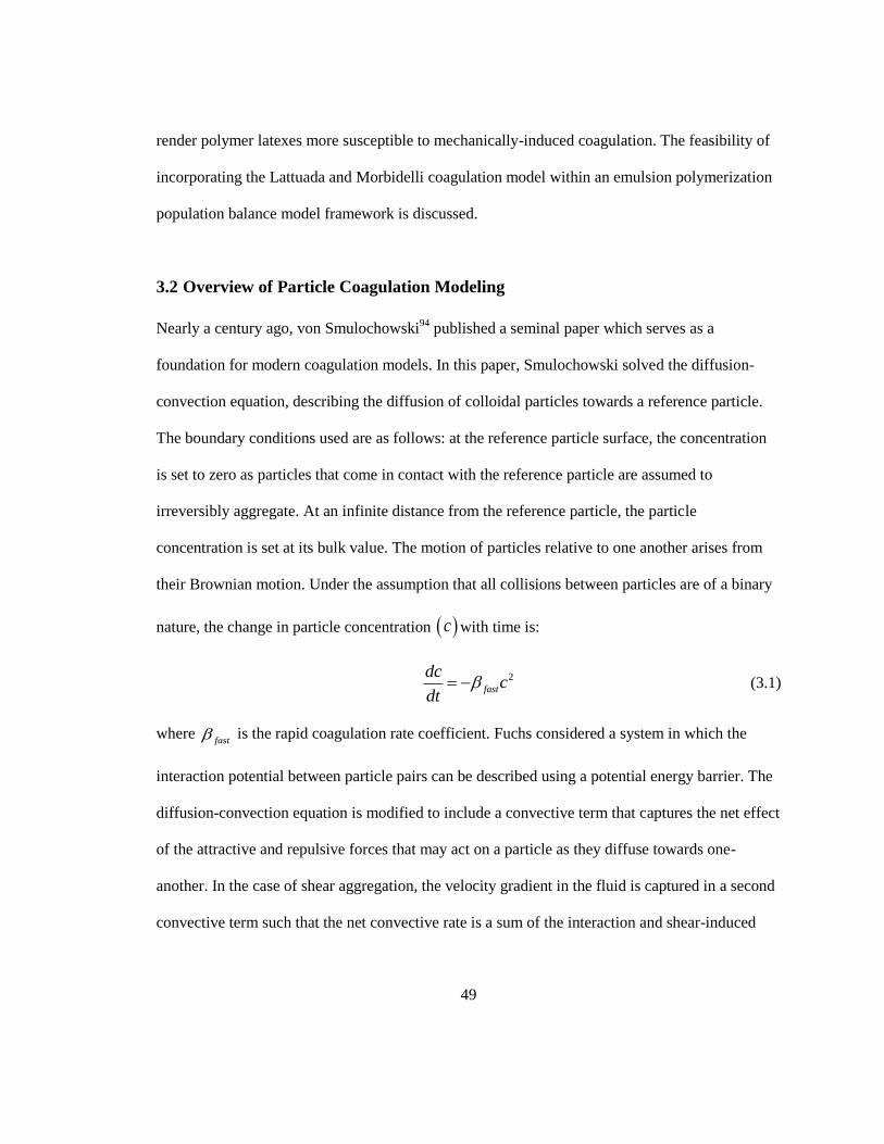
49
render polymer latexes more susceptible to mechanically-induced coagulation. The feasibility of
incorporating the Lattuada and Morbidelli coagulation model within an emulsion polymerization
population balance model framework is discussed.
3.2 Overview of Particle Coagulation Modeling
Nearly a century ago, von Smulochowski94
published a seminal paper which serves as a
foundation for modern coagulation models. In this paper, Smulochowski solved the diffusion-
convection equation, describing the diffusion of colloidal particles towards a reference particle.
The boundary conditions used are as follows: at the reference particle surface, the concentration
is set to zero as particles that come in contact with the reference particle are assumed to
irreversibly aggregate. At an infinite distance from the reference particle, the particle
concentration is set at its bulk value. The motion of particles relative to one another arises from
their Brownian motion. Under the assumption that all collisions between particles are of a binary
nature, the change in particle concentration c with time is:
2
fast
dcc
dt (3.1)
where fast is the rapid coagulation rate coefficient. Fuchs considered a system in which the
interaction potential between particle pairs can be described using a potential energy barrier. The
diffusion-convection equation is modified to include a convective term that captures the net effect
of the attractive and repulsive forces that may act on a particle as they diffuse towards one-
another. In the case of shear aggregation, the velocity gradient in the fluid is captured in a second
convective term such that the net convective rate is a sum of the interaction and shear-induced
50
convective terms. Most modern coagulation models are derived using a variation of the Fuchs-
modified version of the Smoluchowski equation:
int 0convc c D v v (3.2)
where D is the diffusion tensor (modeled as Brownian diffusion and often modified with terms
to account for hydrodynamic interactions), convv is the convective velocity and
intv is the velocity
induced by interparticle interactions. In industrial-scale reactors, convv acting at the particle scale
is modeled as an extensional flow field arising from isotropic turbulence as the latex particles are
smaller than the Kolmogorov scale (the length scale at which the directionality of the turbulent
eddies is lost, typically in the order of a few microns). The following expression is used to
compute convv :
44
2
,
,
1 , 3cos 12
31 , cos sin
2
conv r
conv
rv A r
rv B r
(3.3)
where r is the radial distance from the center of the reference particle and is the colatitude (the
difference between the latitude and 90°) and is the local shear rate. /j ir r is the
dimensionless particle size ratio between the interacting particle pairs, wherej ir r . ,A r
and ,B r are hydrodynamic interaction functions that account for hydrodynamic interactions
between particle pairs in an axisymmetric linear flow field.95
Below the Kolmogorov scale, the
local shear rate can be expressed as a function of the local rate of energy dissipation ( ):
2
15
(3.4)
51
where is the kinematic viscosity.
The interaction velocity vector intv can be modeled using the DLVO theory framework. It must
be noted that the applicability of DLVO theory to modeling emulsion polymerization is
somewhat questionable7 even though it is widely used in the emulsion polymerization modeling
field. Behren et al.96
found that while DLVO theory was quantitatively applicable for weakly
charged particles (i.e. surface charge less than 3 mC/m2) and low ionic strengths (< 10 mM),
discrepancies emerged between theory and experiments at high ionic strengths. An analysis of the
interaction energy profiles suggested that such deviations were closely related to the position of
the energy barrier. At high ionic strengths the energy barrier appears at a separation distance less
than 1 nm and non-DLVO forces (that are not included in the model) become influential. These
non-DLVO forces arise from surface heterogeneities, the discrete nature of charges and the finite
size of ions and water molecules. Since higher ionic strengths and higher surface charges are
typically encountered in emulsion polymerization, the DLVO interaction model should be used
with caution.
Still, the DLVO interaction model is currently the best model available for describing particle
coagulation and non-DLVO forces can be accounted for by making adjustments to certain model
parameters;8 for instance, the Hamaker constant. Under the DLVO framework, intv
may be
computed as follows:
int int
B
Vk T
D
v (3.5)
52
where D is the diffusion tensor, intV is the gradient in the interaction potential,
Bk is the
Boltzmann constant and T is temperature. The diffusion tensor is expressed as a function of the
diffusion coefficient may be modified to account for hydrodynamic interactions that arise
between particle pairs as they approach one another (essentially a form of viscous friction). In
spherical coordinates:
0
, 0 0
0 , 0
0 0 ,
G r
D H r
H r
D (3.6)
where ,G r and ,H r are the radial and angular (polar) hydrodynamic interaction
functions, accounting for resistive forces that arise as particles approach one another. The mutual
diffusion coefficient, 0D is calculated as follows:
0
1 1
6
B
s i j
k TD
r r
(3.7)
where s is the viscosity of the dispersion medium.
As two particles approach one another, fluid must be squeezed out from the gap between the
particles; this action creates a viscous drag on the particles. The hydrodynamic interaction
profiles are typically obtained by numerically solving the equations of motion between pairs of
spherical particles in simple flow fields (for example, see the work of Batchelor and Green95
).
The availability of phenomenological expressions that function in both the near and far field is
limited. In many cases, polynomial fits are used instead; for example, the polynomial function
53
developed by Honig et al.97
for two equal-sized spheres in a dilute solution has seen use in some
particle stability models:
2
2
6 20 16( , 1)
6 11G
(3.8)
The development of an analytical expression for ij that is entirely phenomenological is unlikely
in the near future due to the difficulty in measuring and modeling a number of non-DLVO forces
that are known to be important under certain conditions.98
A simplified coagulation kernel can
still provide reasonable a priori predictive capability through the use of adjustable parameters,
provided the conditions that are being modeled are based on the experimental conditions used to
adjust the model parameters. Within the typical DLVO-based coagulation kernel there are a
number of variables whose values are not known exactly. As stated prior, the Hamaker constant is
typically treated as a semi-empirical parameter, with possible values ranging between
2.0 to 17 × 10-21
J for aqueous polymer latexes.2 The modeler may make slight adjustments to this
parameter to fit experimental data to the model predictions.99, 100
Treated within the DLVO framework, the interaction potential intV is a sum of attractive and
repulsive potentials int A RV V V . The attractive forces are typically lumped together under a
single van der Waals expression:
2 2
2 2 2 2 2 2
2 2 ( )ln
6 ( ) ( ) ( )
i j i j i j
A
i j i j i j
rr rr R r rAV
R r r R r r R r r
(3.9)
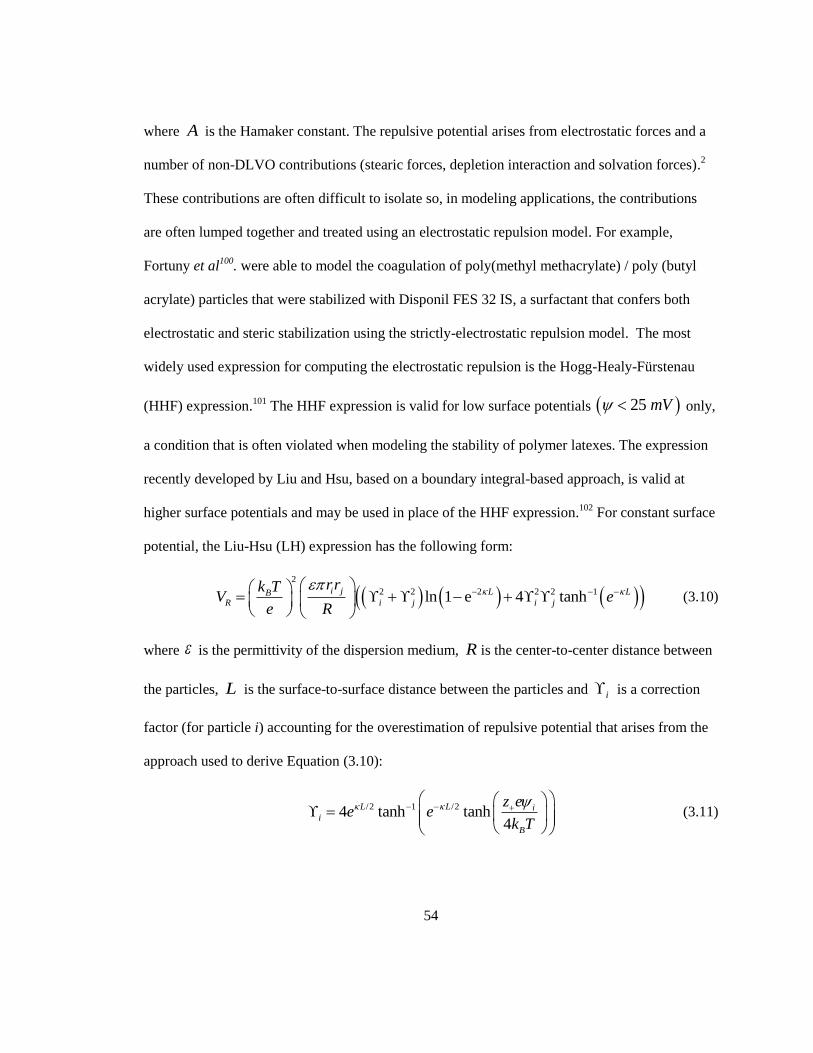
54
where A is the Hamaker constant. The repulsive potential arises from electrostatic forces and a
number of non-DLVO contributions (stearic forces, depletion interaction and solvation forces).2
These contributions are often difficult to isolate so, in modeling applications, the contributions
are often lumped together and treated using an electrostatic repulsion model. For example,
Fortuny et al100
. were able to model the coagulation of poly(methyl methacrylate) / poly (butyl
acrylate) particles that were stabilized with Disponil FES 32 IS, a surfactant that confers both
electrostatic and steric stabilization using the strictly-electrostatic repulsion model. The most
widely used expression for computing the electrostatic repulsion is the Hogg-Healy-Fürstenau
(HHF) expression.101
The HHF expression is valid for low surface potentials 25 mV only,
a condition that is often violated when modeling the stability of polymer latexes. The expression
recently developed by Liu and Hsu, based on a boundary integral-based approach, is valid at
higher surface potentials and may be used in place of the HHF expression.102
For constant surface
potential, the Liu-Hsu (LH) expression has the following form:
2
2 2 2 2 2 1ln 1 e 4 tanhi j L LB
R i j i j
rrk TV e
e R
(3.10)
where is the permittivity of the dispersion medium, R is the center-to-center distance between
the particles, L is the surface-to-surface distance between the particles and i is a correction
factor (for particle i) accounting for the overestimation of repulsive potential that arises from the
approach used to derive Equation (3.10):
/2 1 /24 tanh tanh
4
L L ii
B
z ee e
k T
(3.11)
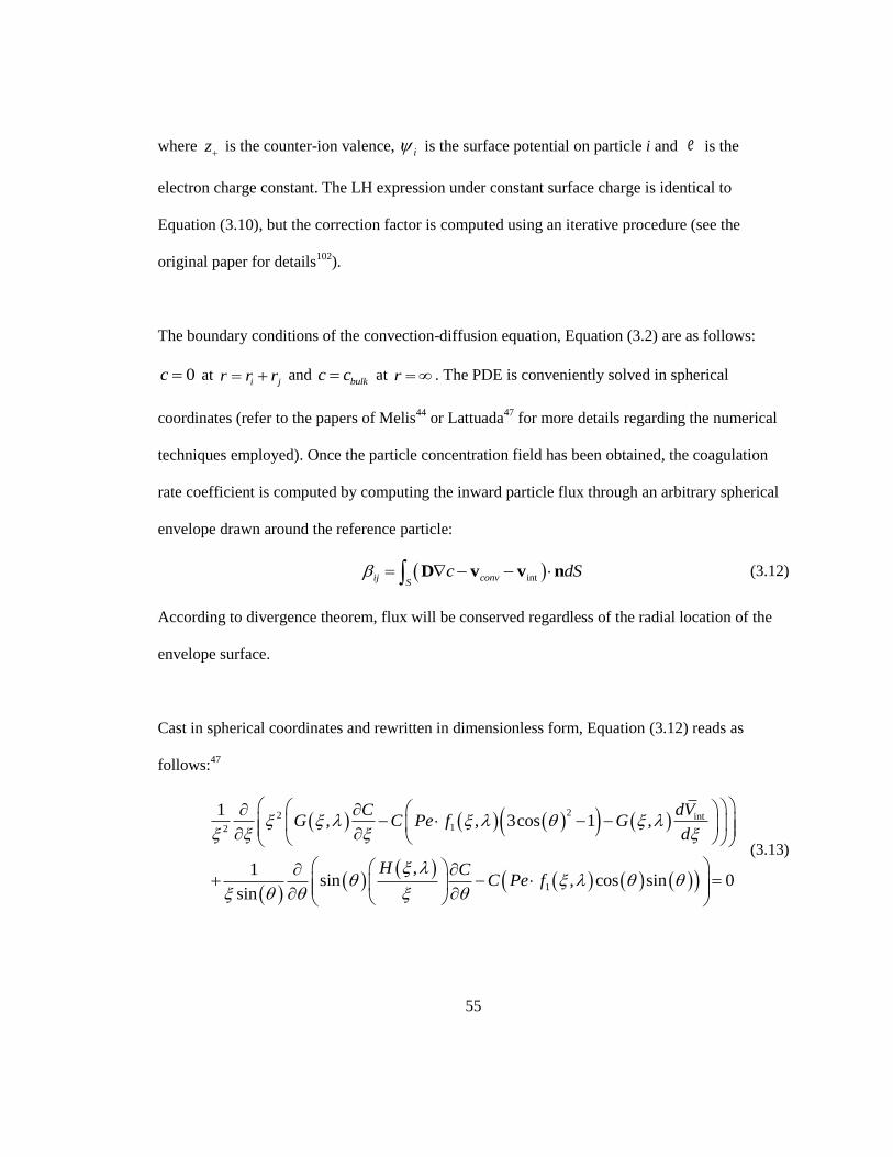
55
where z is the counter-ion valence, i is the surface potential on particle i and e is the
electron charge constant. The LH expression under constant surface charge is identical to
Equation (3.10), but the correction factor is computed using an iterative procedure (see the
original paper for details102
).
The boundary conditions of the convection-diffusion equation, Equation (3.2) are as follows:
0c at i jr r r and
bulkc c at r . The PDE is conveniently solved in spherical
coordinates (refer to the papers of Melis44
or Lattuada47
for more details regarding the numerical
techniques employed). Once the particle concentration field has been obtained, the coagulation
rate coefficient is computed by computing the inward particle flux through an arbitrary spherical
envelope drawn around the reference particle:
intij convS
c dS D v v n (3.12)
According to divergence theorem, flux will be conserved regardless of the radial location of the
envelope surface.
Cast in spherical coordinates and rewritten in dimensionless form, Equation (3.12) reads as
follows:47
22 int12
1
1, , 3cos 1 ,
,1sin , cos sin 0
sin
dVCG C Pe f G
d
H CC Pe f
(3.13)
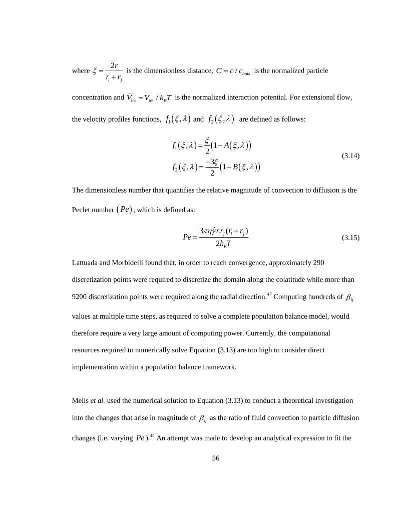
56
where 2
i j
r
r r
is the dimensionless distance, / bulkC c c is the normalized particle
concentration and int int / BV V k T is the normalized interaction potential. For extensional flow,
the velocity profiles functions, 1 ,f and 2 ,f are defined as follows:
1
2
, 1 ,2
3, 1 ,
2
f A
f B
(3.14)
The dimensionless number that quantifies the relative magnitude of convection to diffusion is the
Peclet number Pe , which is defined as:
3 ( )
2
i j i j
B
rr r rPe
k T
(3.15)
Lattuada and Morbidelli found that, in order to reach convergence, approximately 290
discretization points were required to discretize the domain along the colatitude while more than
9200 discretization points were required along the radial direction.47
Computing hundreds of ij
values at multiple time steps, as required to solve a complete population balance model, would
therefore require a very large amount of computing power. Currently, the computational
resources required to numerically solve Equation (3.13) are too high to consider direct
implementation within a population balance framework.
Melis et al. used the numerical solution to Equation (3.13) to conduct a theoretical investigation
into the changes that arise in magnitude of ij as the ratio of fluid convection to particle diffusion
changes (i.e. varying Pe ).44
An attempt was made to develop an analytical expression to fit the
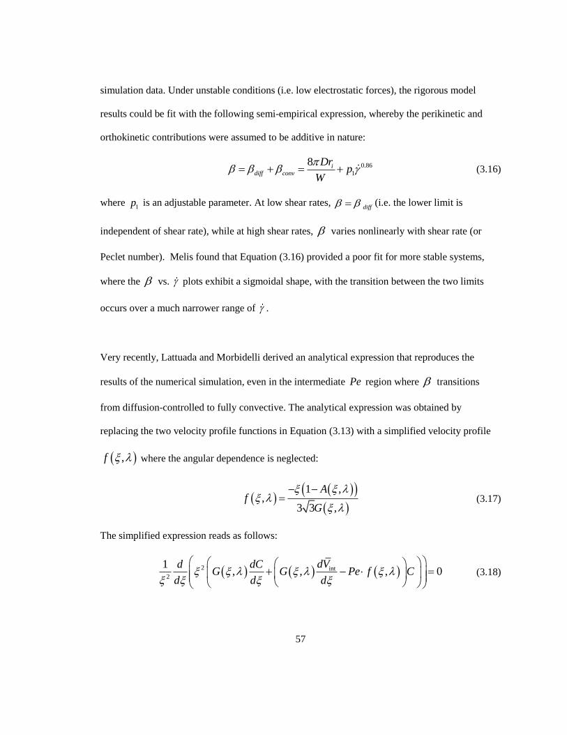
57
simulation data. Under unstable conditions (i.e. low electrostatic forces), the rigorous model
results could be fit with the following semi-empirical expression, whereby the perikinetic and
orthokinetic contributions were assumed to be additive in nature:
0.86
1
8 idiff conv
Drp
W
(3.16)
where 1p is an adjustable parameter. At low shear rates,
diff (i.e. the lower limit is
independent of shear rate), while at high shear rates, varies nonlinearly with shear rate (or
Peclet number). Melis found that Equation (3.16) provided a poor fit for more stable systems,
where the vs. plots exhibit a sigmoidal shape, with the transition between the two limits
occurs over a much narrower range of .
Very recently, Lattuada and Morbidelli derived an analytical expression that reproduces the
results of the numerical simulation, even in the intermediate Pe region where transitions
from diffusion-controlled to fully convective. The analytical expression was obtained by
replacing the two velocity profile functions in Equation (3.13) with a simplified velocity profile
,f where the angular dependence is neglected:
1 ,,
3 3 ,
Af
G
(3.17)
The simplified expression reads as follows:
2 int
2
1, , , 0
dVd dCG G Pe f C
d d d
(3.18)
58
The Lattuada and Morbidelli model requires the use of a boundary layer approximation, as the
expression used to compute the radial velocity will diverge as approaches . Outside of the
boundary layer, the interaction potential is neglected and a simple velocity profile function is
imposed, yielding the following expression:
2
2
1, , 0s
d dCG Pe f C
d d
(3.19)
where /sf and is an adjustable parameter used to capture the size dependence on
the rate of aggregation (arising from hydrodynamic interactions) at high Pe values. The
expression used to compute the boundary layer thickness is:
2
i j
pPe r r
(3.20)
Where p is an adjustable pre-factor that is used to fit the simplified expression‟s predictions to
the numerical data generated from the rigorous solution. Using the Fuchs derivation approach,2
Equation (3.18) is integrated from 2 to 2 and Equation (3.19) is integrated from
2 to , obtaining an expression for ij . Expressed in terms of a stability ratio, W :
int
22 ( ) ( 2 )
2
22
1
2,
ij
fast dVHe Pe f d Pe Pe Heij d
W
ed
G
(3.21)
where He x is the Heaviside function and ij is the diffusion-limited rate of aggregation:
, ,
, ,
2 1 1
3
B s i s jfast
ij
s i s j
k T r r
r r
(3.22)
59
The presence of two adjustable parameters in Equation (3.21) may limit its applicability, but it
captures the sigmoidal shape of the stability curve that is predicted by the rigorous expression. In
the presence of particle interaction (e.g. for latex particles that are stabilized by adsorbed
surfactant), but no fluid convection ( 0Pe ), Equation (3.23) simplifies to the following
expression:
int ( , )
222
( , )
fast
ij
ij Ve
dG
(3.23)
The denominator of Equation (3.23) is the Fuchs stability ratio (W ). Equation (3.23) has found
widespread use in emulsion polymerization modeling field8, 99, 103, 104
where it is typically assumed
that fluid convection on the microscopic scale can be neglected. If the complex velocity function
is replaced by a symmetrical velocity gradient ,conv rv r , the following expression can be
obtained (refer to section 4.6.1.3 of Blackley2 for the derivation):
.1 ,2int
22
1
4exp
32
,
ij
fast
ij s s
B
Pe r rV
k Td
G
(3.24)
3.3 Outline of CFD Simulation Method
The reactor investigated in this work was a round-bottom vessel agitated by a centered four-
bladed 45° pitched blade turbine with two round baffles. The reactor geometry considered in this
work is shown in Figure 3.1, along with the key vessel and impeller dimensions. While the
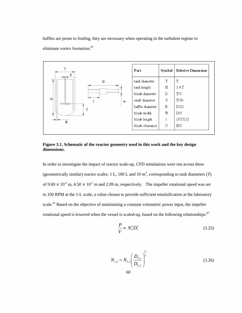
60
baffles are prone to fouling, they are necessary when operating in the turbulent regime to
eliminate vortex formation.87
Figure 3.1. Schematic of the reactor geometry used in this work and the key design
dimensions.
In order to investigate the impact of reactor scale-up, CFD simulations were run across three
(geometrically similar) reactor scales: 1 L, 100 L and 10 m3, corresponding to tank diameters (T)
of 9.69 × 10⁻²
m, 4.50 × 10⁻¹
m and 2.09 m, respectively. The impeller rotational speed was set
to 100 RPM at the 1-L scale, a value chosen to provide sufficient emulsification at the laboratory
scale.41
Based on the objective of maintaining a constant volumetric power input, the impeller
rotational speed is lowered when the vessel is scaled-up, based on the following relationships:87
3 2
I I
PN D
V (3.25)
2
3,1
,2 ,1
,2
I
I I
I
DN N
D
(3.26)
61
Application of Equation (3.26) results in the impeller rotational speed being lowered to
(approximately) 35.9 RPM and 12.2 RPM as the reactor is scaled-up to 100 L and 10 m3,
respectively. Equation (3.25) holds true for turbulent conditions only, where inertial forces
dominate.
The base case reactor fluid modeled is a 44 vol.-% solids content polymer latex, with an average
particle diameter of 150 nm and a particle polydispersity index of 0.10 (narrowly distributed). An
additional set of simulations were run in which the solids content of the latex was increased to ~
60 vol.-% in order to examine the effect of solids content on the shear rate distribution inside the
reactor. Latex viscosity was modeled using the Carreau-Yasuda model, which has been shown to
correctly capture the shearing behavior of concentrated latexes;5
0
1 / for
1thm a
a
(3.27)
where 0 is the zero-shear viscosity,
is the infinite-shear viscosity, is the characteristic
time for the onset of shear-thinning and th is the shear rate beyond which the latex will begin to
shear thicken. Pishvaei found that setting the values of the adjustable parameters, a and m , to 1.0
and 0.65, respectively, provided the best fit to their experimental data. The four model parameters
are dependent on the latex solid content and the (PSD-dependent) effective maximum
packing fraction m according to general form of the Krieger-Dougherty equation.58
,
0
,
1 , , , 1/
m
s th
m
(3.28)
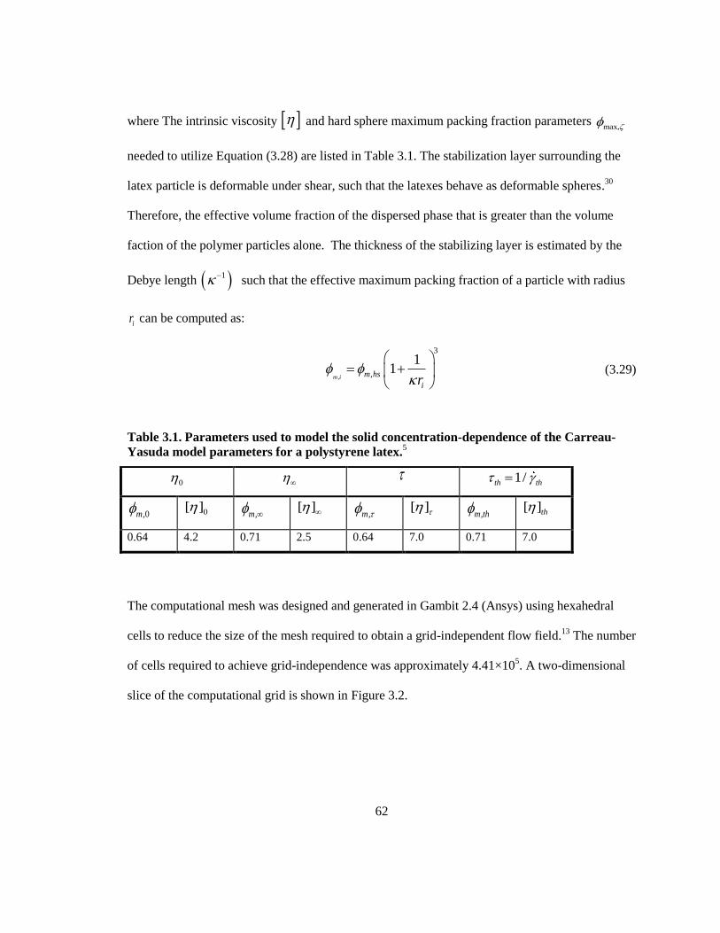
62
where The intrinsic viscosity and hard sphere maximum packing fraction parameters max,
needed to utilize Equation (3.28) are listed in Table 3.1. The stabilization layer surrounding the
latex particle is deformable under shear, such that the latexes behave as deformable spheres.30
Therefore, the effective volume fraction of the dispersed phase that is greater than the volume
faction of the polymer particles alone. The thickness of the stabilizing layer is estimated by the
Debye length 1 such that the effective maximum packing fraction of a particle with radius
ir can be computed as:
,
3
,
11
m i m hs
ir
(3.29)
Table 3.1. Parameters used to model the solid concentration-dependence of the Carreau-
Yasuda model parameters for a polystyrene latex.5
0 1/th th
,0m 0[ ] ,m [ ]
,m [ ]
,m th [ ]th
0.64 4.2 0.71 2.5 0.64 7.0 0.71 7.0
The computational mesh was designed and generated in Gambit 2.4 (Ansys) using hexahedral
cells to reduce the size of the mesh required to obtain a grid-independent flow field.13
The number
of cells required to achieve grid-independence was approximately 4.41×10⁵. A two-dimensional
slice of the computational grid is shown in Figure 3.2.
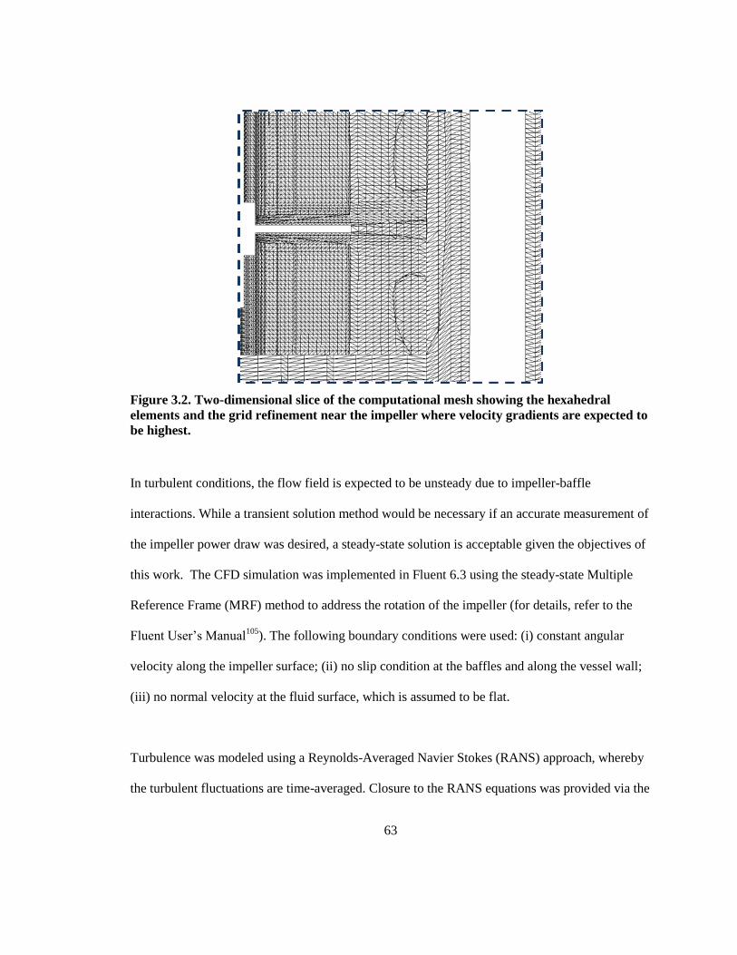
63
Figure 3.2. Two-dimensional slice of the computational mesh showing the hexahedral
elements and the grid refinement near the impeller where velocity gradients are expected to
be highest.
In turbulent conditions, the flow field is expected to be unsteady due to impeller-baffle
interactions. While a transient solution method would be necessary if an accurate measurement of
the impeller power draw was desired, a steady-state solution is acceptable given the objectives of
this work. The CFD simulation was implemented in Fluent 6.3 using the steady-state Multiple
Reference Frame (MRF) method to address the rotation of the impeller (for details, refer to the
Fluent User‟s Manual105
). The following boundary conditions were used: (i) constant angular
velocity along the impeller surface; (ii) no slip condition at the baffles and along the vessel wall;
(iii) no normal velocity at the fluid surface, which is assumed to be flat.
Turbulence was modeled using a Reynolds-Averaged Navier Stokes (RANS) approach, whereby
the turbulent fluctuations are time-averaged. Closure to the RANS equations was provided via the
64
standard k model, which has been shown to provide acceptable agreement with
experimental results, particularly with regards to the overall flow field.74, 106
Deglon and Meyer107
found that the MRF method coupled with the k turbulence model could accurately model the
fine scale turbulent structures (including the trailing vortices) in a stirred tank, however, a high
grid resolution (~ 2 × 10⁶ cells) was required. The turbulence models included in the Fluent
commercial CFD simulation package were developed for modeling Newtonian fluids; that is,
fluids with shear-rate independent viscosity. The RANS approach to turbulence modeling
requires the decomposition of instantaneous variables (e.g. velocity, pressure) into mean and
fluctuating components. The additional fluctuating terms (known as Reynolds stresses) that show
up in the conservation equations require the derivation of additional conservation equations to
provide closure. In the k-ε model, closure is provided through the specification of two additional
conservation equations: one for kinetic energy ( k ) and one for turbulent energy dissipation (ε).11
For non-Newtonian fluids, the conservation equations include extra stress terms, sometimes
referred to as polymeric stresses, due to fluctuations in apparent viscosity. The classic k
model does not take these extra source terms into account, so the predictive capabilities of
Newtonian turbulence models, as applied to non-Newtonian fluids, is questionable. Since the
closure of RANS equations for non-Newtonian fluids is still a topic of current research,108
it is
unlikely that commercial CFD software will include specialized turbulence models for non-
Newtonian fluids in the near future. While there has been some progress in modeling the
turbulent flow of non-Newtonian fluids using Direct Numerical Simulation (DNS),109
the
computational requirements of DNS are still highly restrictive. Therefore, the modeling of fluid
rheology under fully turbulent flow for non-Newtonian fluids inside stirred vessels requires the
use of an approximate method. The most-commonly applied approach is the Metzner-Otto
65
method, whereby a constant apparent viscosity is employed in lieu of a non-Newtonian viscosity
model; the apparent viscosity is computed using a representative shear rate via Equation (3.4).
The Metzner-Otto method has been shown to provide acceptable predictions when used to model
turbulent mixing of non-Newtonian fluids inside reactors, 17, 74, 106
although strictly speaking, it
was developed for reactors in the laminar regime.110
Recently, Wu and Chen modeled the flow
inside an anaerobic digester using a power-law viscosity model in conjunction with the standard
k turbulence model and found that the model‟s predictive capabilities were acceptable.111
Based on the findings of Wu and Chen, the decision was made to proceed with the use of the
Carreau-Yasuda model to compute fluid viscosity, with a secondary set of simulations being run
for comparison by replacing the non-Newtonian rheological model with an apparent viscosity
(computed using the Metzner-Otto approach):
0
1 /
1aa m a
aKN
(3.30)
where K is an adjustable proportionality constant..
Although it is often misapplied to a wider range of flow conditions, the Metzner-Otto method was
designed (and validated) strictly as a means of computing power consumption for mixing tanks
operating in the laminar regime, where the Power number is inversely proportional to the
Reynolds number. For fully-turbulent flow, the high rate of energy dissipation in the impeller
region generates additional shear (refer to Equation (3.4)) such that the contributions of
turbulence to shear may be at least one order of magnitude greater than the contribution from the
mean velocity field gradient.110
In such a scenario, the Metzner-Otto method will under-
66
approximate the shear field within the impeller region. To account for shear generated through
the dissipation of the smallest eddies, Nouri and Hockey112
recommended setting the
proportionality constant, K , to 54, which is outside the range of 10 – 12 recommended for the
computation of power consumption in the laminar regime.87
While this adjustment may yield a
better fit for computing the power consumption, the Metzner-Otto method is still inappropriate
for modeling liquid blending because the shear rate outside of the impeller region will be orders
of magnitude lower. The increase in the proportionality constant meant to extend the Metzner-
Otto method‟s applicability to operation in the transition and turbulent regimes will exacerbate
the overestimation of shear within the region far away from the impeller, thus underestimating
blend time. Thus from the perspective of blend performance, the predictions generated using the
Metzner-Otto approximation for dynamic viscosity can be thought of as an optimistic scenario
(i.e. an underestimation of the blend time).
3.4 Results and Discussion
3.4.1 CFD Simulation Results
At 44 vol.-% solids, the computed rheological parameters of the latex were as follows:
2 3
0
2
2.05 10 kg/m/s 5.67 10 kg/m/s
1/ 1.96 10 sth
Using 0 and
, a Reynolds number operating range can be estimated as
2 2
min max
0
Re ReND ND
(3.31)
67
The computed Reynolds number (Re) ranges are:
2 3
3 4
3 4 5
1L: 7.63 10 2.76 10
100 L: 5.89 10 2.13 10
10 m : 4.31 10 1.56 10
Using the rule-of-thumb guideline that a reactor is operating in the transitional regime when
2 410 Re 10 and fully-turbulent regime when 4Re 10 , the 10 m
3 reactor is the only reactor
scale which is operating under fully-turbulent conditions, while the laboratory and pilot scale
reactors are operating in the transitional regime. The computed power numbers PN were as
follows:
1
1
3 1
1L: 6.87 10
100 L: 5.01 10
10 m : 4.56 10
P
P
P
N
N
N
For pitched blade turbines,87
13 10PN , which is reasonably close to the value computed at
the 10 m3-scale. It can be seen from the computed
PN values (above) that they are decreasing
with Re , which further suggests that the lab and pilot scale reactors are not operating in the fully
turbulent regime, as PN is independent of Re in the fully-turbulent regime. This conclusion is
reinforced when the flow profiles along a vertical cross section cut through the center of the
vessel (Figure 3.3) are examined. It can be seen that the flow pattern predicted at the 1-L scale
differs to a large degree from the predicted flow patterns seen at the 100 – L and 10-m3 scales.
The change in flow profile with vessel scale does not provide much insight towards the study of
mechanically induced particle coagulation, beyond establishing the expectation that the shear rate
distribution will change with the reactor scale. Using Equation (3.4), the local shear rate
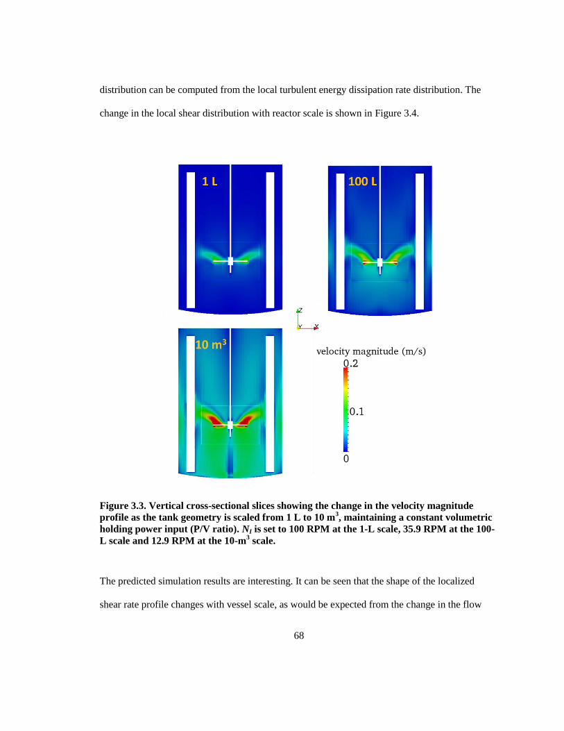
68
distribution can be computed from the local turbulent energy dissipation rate distribution. The
change in the local shear distribution with reactor scale is shown in Figure 3.4.
Figure 3.3. Vertical cross-sectional slices showing the change in the velocity magnitude
profile as the tank geometry is scaled from 1 L to 10 m3, maintaining a constant volumetric
holding power input (P/V ratio). NI is set to 100 RPM at the 1-L scale, 35.9 RPM at the 100-
L scale and 12.9 RPM at the 10-m3 scale.
The predicted simulation results are interesting. It can be seen that the shape of the localized
shear rate profile changes with vessel scale, as would be expected from the change in the flow
69
profile. The volume-averaged turbulent shear rate decreases as the vessel is scaled up from 1 L to
10 m3. Computed over the entire domain, the volume-averaged (turbulence-induced) shear rate
decreases from 7.9 s-1
at the 1-L scale to 5.4 s-1
at 10-m3 scale. The maximum shear rate in the
flow (due to turbulence) is 1250 s-1
at the 1-L scale and 134.9 s-1
at the 10 m3-scale. In addition to
the extensional flow generated from the smallest turbulent eddies, the shear at the impeller tips
should be briefly considered as well. Unfortunately the mesh resolution at the impeller tips is not
fine enough to determine the shear rate precisely, but heuristic guidelines propose the following
scaling relationship:
max (= tip speed)ND
From the 1–L to the 10-m3 scale, the maximum shear arising from the fluid velocity gradient is
expected to increase by a factor of ~ 2.8, although Melis notes that the inertial forces from the
main flow field can be neglected for particles that are smaller than a few microns (i.e. at the
microscopic particle scale, the shear arising from the Kolmogorov scale turbulence is more
important).44
Furthermore, it should be noted that this expression does not account for the high
rate of shear generated from turbulence in the trailing vortices near the impeller tips, which is
likely to be higher. 84
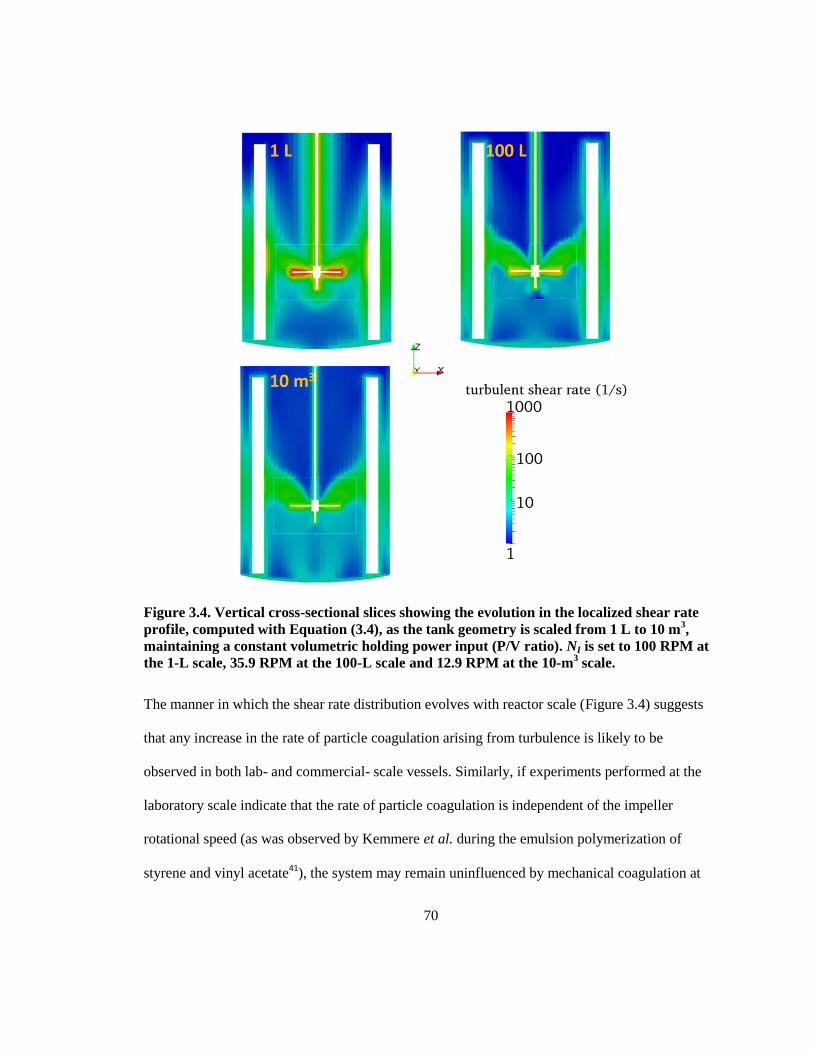
70
Figure 3.4. Vertical cross-sectional slices showing the evolution in the localized shear rate
profile, computed with Equation (3.4), as the tank geometry is scaled from 1 L to 10 m3,
maintaining a constant volumetric holding power input (P/V ratio). NI is set to 100 RPM at
the 1-L scale, 35.9 RPM at the 100-L scale and 12.9 RPM at the 10-m3 scale.
The manner in which the shear rate distribution evolves with reactor scale (Figure 3.4) suggests
that any increase in the rate of particle coagulation arising from turbulence is likely to be
observed in both lab- and commercial- scale vessels. Similarly, if experiments performed at the
laboratory scale indicate that the rate of particle coagulation is independent of the impeller
rotational speed (as was observed by Kemmere et al. during the emulsion polymerization of
styrene and vinyl acetate41
), the system may remain uninfluenced by mechanical coagulation at
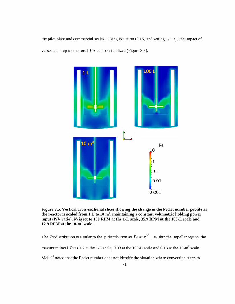
71
the pilot plant and commercial scales. Using Equation (3.15) and setting i jr r , the impact of
vessel scale-up on the local Pe can be visualized (Figure 3.5).
Figure 3.5. Vertical cross-sectional slices showing the change in the Peclet number profile as
the reactor is scaled from 1 L to 10 m3, maintaining a constant volumetric holding power
input (P/V ratio). NI is set to 100 RPM at the 1-L scale, 35.9 RPM at the 100-L scale and
12.9 RPM at the 10-m3 scale.
The Pe distribution is similar to the distribution as 1/2Pe . Within the impeller region, the
maximum local Pe is 1.2 at the 1-L scale, 0.33 at the 100-L scale and 0.13 at the 10-m3 scale.
Melis44
noted that the Peclet number does not identify the situation where convection starts to
72
play a role, but modified Peclet number Pe does and can be computed for equal radii particles
with the following expression:
2
1 s
s
rPe Pe
r
(3.32)
Since the modified Peclet number depends on the inverse Debye length, more detailed reaction
conditions must be specified before Pe can be computed. For example, at 44 vol..-% solids
content, a sodium dodecyl sulphate concentration of 5.3×10⁻³
wt.-% and a sodium chloride salt
concentration of 2.65×10⁻²
wt.-%, 1 91.05 10 m . For
87.5 10 mr , r 75 and
/ 74Pe Pe . Under these conditions, Pe takes on the following maximum values:
2 3 31 L reactor : 1.7 10 10 m reactor : 2.0 10Pe Pe
If the surfactant and salt concentrations are drastically reduced, 1 would increase.
1 83 10 m is a realistic upper limit, which corresponds to corresponding to r 2.5 and
/1.79Pe Pe . Under these conditions, the maximum value of Pe in the reactors is:
1 3 21 L reactor : 7.2 10 10 m reactor : 8.4 10Pe Pe
In the 1-L reactor, Pe is above the threshold of 0.1Pe , which according to Melis44
, indicates
that the reactor fluid dynamics are likely to play a role in the aggregation rate.
A direct relationship between Pe and r can be obtained by setting 1 2r r r in Equation
(3.15) and substituting the resulting expression into Equation (3.32):
2
13 s
b
rrPe
k T
(3.33)
73
This indicates that Pe increases in proportion to 2r r and in inverse proportion to 2 .
According to Equation (3.33), if the aggregation of 150 nm particles is influenced by the shear
field in the impeller region, then the aggregation rate of particles larger than 150 nm in diameter
would be affected in a larger region of the reactor. Equation (3.33) also indicates that latexes
may become more sensitive to shear under conditions where the double layer is diffuse (i.e. an
environment of low ionic strength). Therefore, shear-induced coagulation may or may not
enhance the rate of particle coagulation at both the laboratory scale and the industrial scales,
depending on the reactor conditions and the latex particle size distribution. Therefore it is not
surprising to find conflicting conclusions regarding the importance of shear-induced coagulation
throughout the literature.41, 45
Interestingly, the latex may become more sensitive to mechanical
agitation under conditions where the latex is stabilized against Brownian coagulation. In reactors
where the latex is purposefully destabilized through the addition of an electrolyte (thereby raising
the ionic strength) the flow field is unlikely to enhance the rate of particle aggregation.
Due to the difficulty faced in modeling non-Newtonian fluids in the turbulent regime, it is useful
to investigate the effect of the viscosity modeling approach on the qualitative CFD predictions.
An additional set of simulations were run, where the Carreau-Yasuda model was used in place of
the Metzner-Otto approximation to model the apparent viscosity of a 44 vol.-% latex. At 44 vol.-
%, the difference between the viscosity limits is on the order of 3.5, thus is not surprising to
observe that the qualitative characteristics of the flow fields does not change appreciably between
the two approaches to modeling fluid viscosity. The velocity magnitude profiles are show in
Figure 3.6, while the particle Pe distribution profiles are shown in Figure 3.7. At 44 vol.-%
solids content, the choice of fluid viscosity model does not appear to have an appreciable effect
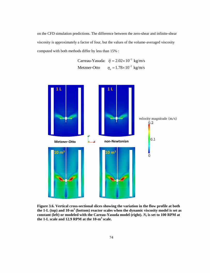
74
on the CFD simulation predictions. The difference between the zero-shear and infinite-shear
viscosity is approximately a factor of four, but the values of the volume-averaged viscosity
computed with both methods differ by less than 15% :
2
2
Carreau-Yasuda: 2.02 10 kg/m/s
Metzner-Otto 1.78 10 kg/m/sa
Figure 3.6. Vertical cross-sectional slices showing the variation in the flow profile at both
the 1-L (top) and 10-m3 (bottom) reactor scales when the dynamic viscosity model is set as
constant (left) or modeled with the Careau-Yasuda model (right). NI is set to 100 RPM at
the 1-L scale and 12.9 RPM at the 10-m3 scale.
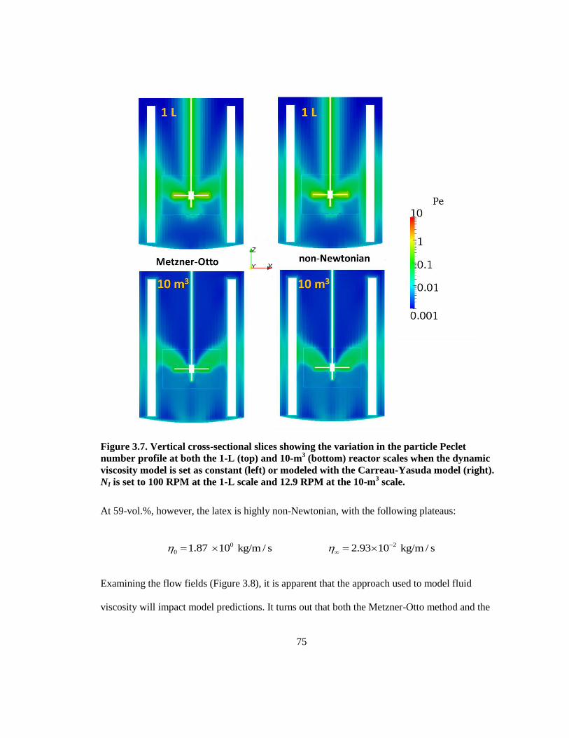
75
Figure 3.7. Vertical cross-sectional slices showing the variation in the particle Peclet
number profile at both the 1-L (top) and 10-m3 (bottom) reactor scales when the dynamic
viscosity model is set as constant (left) or modeled with the Carreau-Yasuda model (right).
NI is set to 100 RPM at the 1-L scale and 12.9 RPM at the 10-m3 scale.
At 59-vol.%, however, the latex is highly non-Newtonian, with the following plateaus:
0 2
0 1.87 10 kg/m / s 2.93 10 kg/m / s
Examining the flow fields (Figure 3.8), it is apparent that the approach used to model fluid
viscosity will impact model predictions. It turns out that both the Metzner-Otto method and the
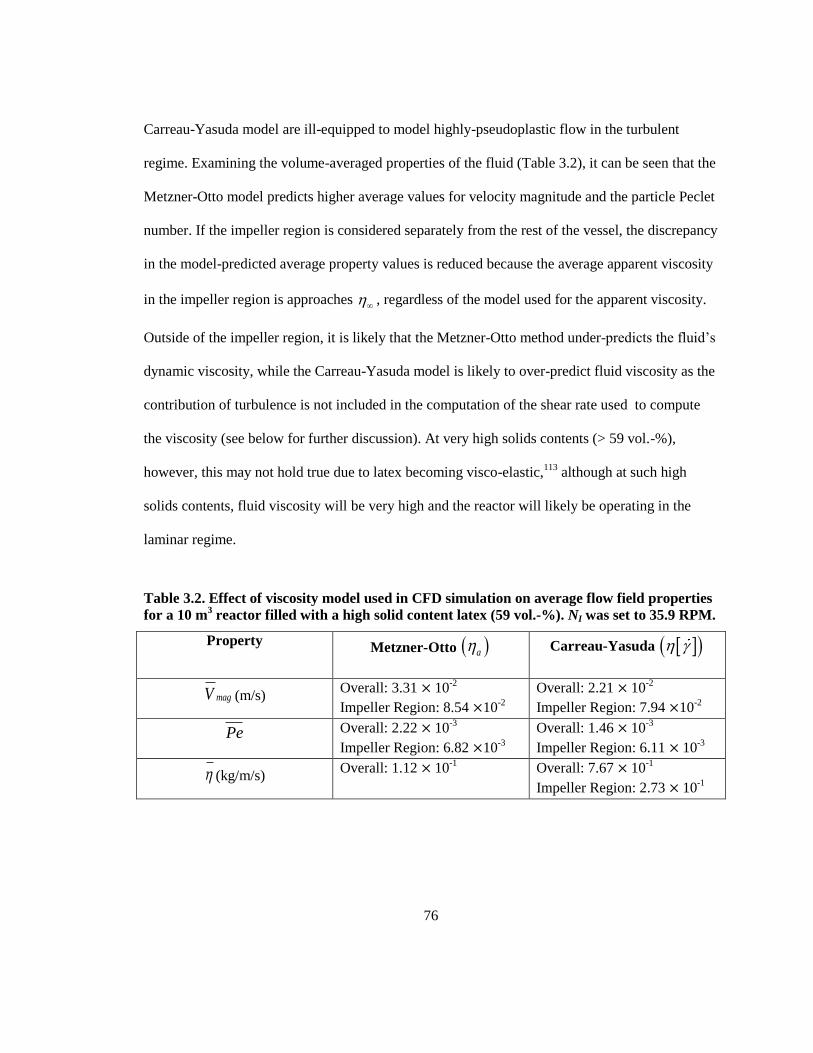
76
Carreau-Yasuda model are ill-equipped to model highly-pseudoplastic flow in the turbulent
regime. Examining the volume-averaged properties of the fluid (Table 3.2), it can be seen that the
Metzner-Otto model predicts higher average values for velocity magnitude and the particle Peclet
number. If the impeller region is considered separately from the rest of the vessel, the discrepancy
in the model-predicted average property values is reduced because the average apparent viscosity
in the impeller region is approaches , regardless of the model used for the apparent viscosity.
Outside of the impeller region, it is likely that the Metzner-Otto method under-predicts the fluid‟s
dynamic viscosity, while the Carreau-Yasuda model is likely to over-predict fluid viscosity as the
contribution of turbulence is not included in the computation of the shear rate used to compute
the viscosity (see below for further discussion). At very high solids contents (> 59 vol.-%),
however, this may not hold true due to latex becoming visco-elastic,113
although at such high
solids contents, fluid viscosity will be very high and the reactor will likely be operating in the
laminar regime.
Table 3.2. Effect of viscosity model used in CFD simulation on average flow field properties
for a 10 m3 reactor filled with a high solid content latex (59 vol.-%). NI was set to 35.9 RPM.
Property Metzner-Otto a
Carreau-Yasuda
magV (m/s) Overall: 3.31 × 10
-2
Impeller Region: 8.54 ×10⁻²
Overall: 2.21 × 10⁻²
Impeller Region: 7.94 ×10⁻²
Pe Overall: 2.22 × 10⁻³
Impeller Region: 6.82 ×10⁻³
Overall: 1.46 × 10⁻³
Impeller Region: 6.11 × 10⁻³
(kg/m/s) Overall: 1.12 × 10
-1
Overall: 7.67 × 10⁻¹
Impeller Region: 2.73 × 10⁻¹
77
Figure 3.8. Vertical cross-sectional slices showing, for a higher solids content (59 vol.-%),
the differences in the velocity profile (top) and the particle Peclet number profile when the
dynamic viscosity model is changed from a constant approximation (left) to the Carreau-
Yasuda (right). NI is set to 12.9 RPM.
Direct implementation of a non-Newtonian viscosity law within the CFD code presents its own
set of issues that call into question the quality of the predictions. Within the impeller region, the
amount of shear acting upon the fluid is likely to be underestimated as the shear rate used to
compute the fluid viscosity does not include any additional shear that may arise from the
turbulent eddies. On the other hand, the Newtonian RANS models are expected to overestimate
78
the amount of turbulence present for a given set of flow conditions. As mentioned prior, the
Newtonian turbulence closure models do not account for local fluctuations in the fluid viscosity.
These fluctuations, if modeled as polymeric stress terms, would act opposite the Reynolds
stresses; that is, if the Reynolds stresses transfer energy from the mean flow to increase the
fluctuating components, the polymer stresses would reduce this effect.108
Since the Carreau-
Yasuda model implemented neglects the shear field arising from the dissipation of turbulence
entirely, fluid viscosity is likely to be over-estimated. To further complicate matters, as the
particle concentration in a latex approaches the maximum packing fraction, the latex will begin to
display viscoelastic behavior113
. The high viscosity coupled with viscoelasticity may lead to
cavern formation, whereby mixing is confined to a small region around the impeller and the fluid
outside this region will remain stagnant. Taking all of these factors into consideration, it would be
unwise to rely upon CFD simulation, in its current state of development (commercial or
otherwise), to model the mixing of high solid content polymer latexes at the commercial scale,
where turbulence may be present yet confined to a small cavernous region surrounding the
impeller.
3.4.2 Comparison of simple shear model vs. rigorous solution to the convection-diffusion
equations
Lattuada and Morbidelli recently presented an expression for computing coagulation rate
coefficients (Equation (3.21)) that reproduces the results obtained from the rigorous numerical
solution to the Fuchs-Smoluchowski convection-diffusion equation in two dimensions. A
coagulation model that can be used at both low and high Pe would be particularly useful for
modeling industrial emulsion polymerization reactions from start to finish, where fluid rheology
79
and ionic conditions may vary by orders of magnitude over the course of the reaction. The results
of Figure 3 of Lattuada and Morbidelli are reproduced below in Figure 3.9 (the lines with
symbols).
Examining the curves produced using the Lattuada and Morbidelli model in Figure 3.9, one is
drawn to the counterintuitive relationship between the ionic strength of the dispersion medium
and the critical Pe at which the orthokinetic coagulation begins to contribute to (and eventually
dominate) the overall rate of coagulation. As ionic strength is increased, both Equation (3.21) and
the rigorous numerical simulation indicate that, while the system will become more susceptible to
Brownian coagulation at the low shear limit, the critical Pe at which the system becomes
susceptible to the effect of the shear field will increase. This falls in line with the trend predicted
by Equation (3.33). Lattuada and Morbidelli reasoned that the magnitude of the electrostatic force
intF is inversely proportional to the thickness of the double layer int int e LF V ;
therefore, a thicker double layer (and hence smaller ) results in the magnitude of the
electrostatic force being smaller. From Equation (3.5) it can be seen that the velocity contribution
due to interaction potential intv is proportional to the electrostatic force, thus it too will
decrease in magnitude if is decreased and its contribution to the overall convective flux will be
smaller. As a result, a weaker convective contribution convv is needed to transition from the
DLVO-controlled regime to the convective or shear-controlled regime. When the double layer
thickness is decreased, the low Pe aggregation rate will increase due to a reduction in the
electrostatic energy barrier, but the electrostatic forces will increase, leading to the regime
transition occurring at a higher Pe .47
The curves generated under the same conditions using the
80
simple shear coagulation model (Equation (3.24)) do not show this trend, despite having a very
similar form to Equation (3.21); in fact, Equation (3.24) predicts that the Pe at which transition
occurs is independent of ionic strength.
Examining Equation (3.21) in more detail, there are a number of components that set it apart from
the simpler expression, Equation (3.24). The most significant difference between the two models
is the inclusion of the boundary layer approximation in Equation (3.24). When the dimensionless
distance of particle separation is less than the dimensionless thickness of the boundary layer, the
total potential between the particles is computed by integrating the following expression:
int
2 2
dVPe f d Pe
dt
(3.34)
Slight rearrangement of this expression, coupled with substitution of the appropriate
hydrodynamic function for extensional flow (Equation (3.17)) results in the following
expression:47
int int2
1 ,( )
23 3 ,
APe d V V
G
(3.35)
As the thickness of the double layer increases, will likewise increase. As , the first
term of Equation (3.35) (and indeed, the entire expression) will approach . Recall that the
first term arises from the use of a diverging velocity field. The further the boundary layer is
extended outwards, the greater the influence of the convective potential and the lower the Pe at
which the convective contribution becomes important. Numerically, it is the changes in the
convective potential, rather than the interactive potential that result in the slightly counterintuitive
trend seen in Figure 3.9. The velocity field function in Equation (3.24) is similar in to the velocity
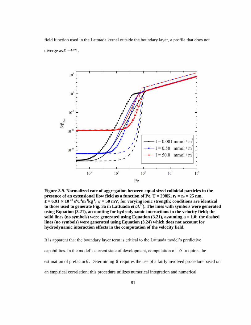
81
field function used in the Lattuada kernel outside the boundary layer, a profile that does not
diverge as .
Figure 3.9. Normalized rate of aggregation between equal sized colloidal particles in the
presence of an extensional flow field as a function of Pe. T = 298K, r1 = r2 = 25 nm,
𝛆 = 6.91 × 10⁻¹⁰
s2C
2m
-1kg
-1, ψ = 50 mV, for varying ionic strength; conditions are identical
to those used to generate Fig. 3a in Lattuada et al.47
). The lines with symbols were generated
using Equation (3.21), accounting for hydrodynamic interactions in the velocity field; the
solid lines (no symbols) were generated using Equation (3.21), assuming a = 1.0; the dashed
lines (no symbols) were generated using Equation (3.24) which does not account for
hydrodynamic interaction effects in the computation of the velocity field.
It is apparent that the boundary layer term is critical to the Lattuada model‟s predictive
capabilities. In the model‟s current state of development, computation of requires the
estimation of prefactor a . Determining a requires the use of a fairly involved procedure based on
an empirical correlation; this procedure utilizes numerical integration and numerical
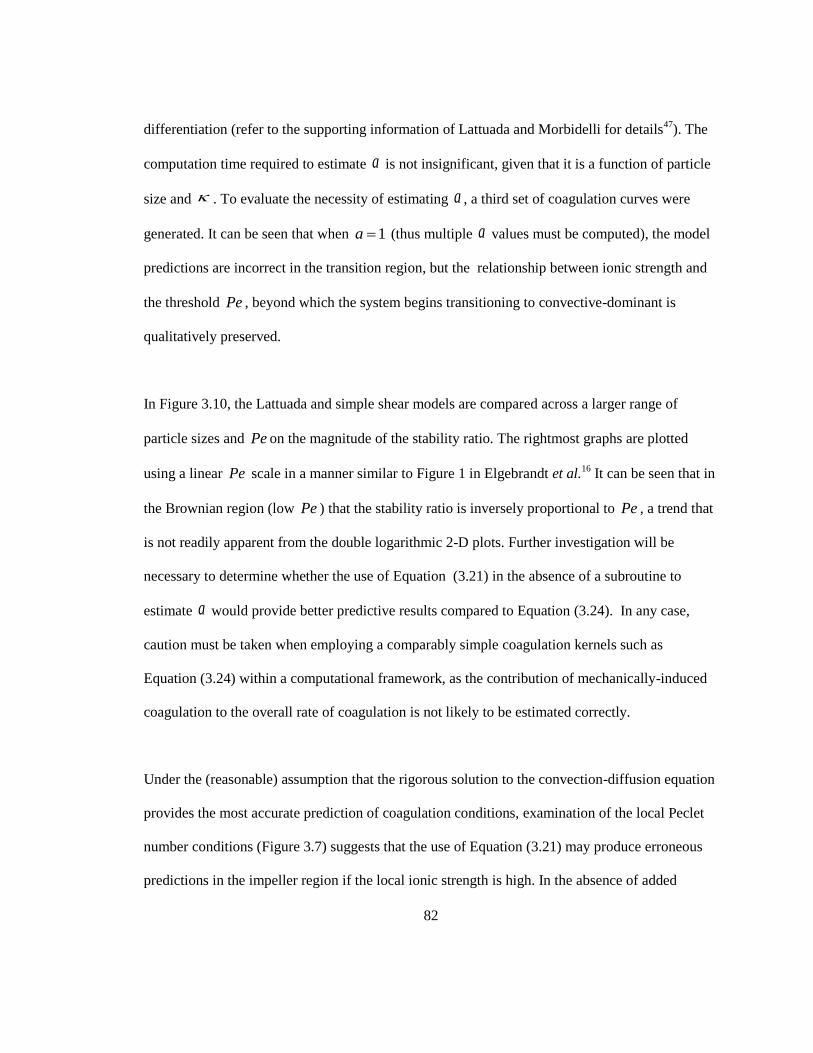
82
differentiation (refer to the supporting information of Lattuada and Morbidelli for details47
). The
computation time required to estimate a is not insignificant, given that it is a function of particle
size and . To evaluate the necessity of estimating a , a third set of coagulation curves were
generated. It can be seen that when 1a (thus multiple a values must be computed), the model
predictions are incorrect in the transition region, but the relationship between ionic strength and
the threshold Pe , beyond which the system begins transitioning to convective-dominant is
qualitatively preserved.
In Figure 3.10, the Lattuada and simple shear models are compared across a larger range of
particle sizes and Pe on the magnitude of the stability ratio. The rightmost graphs are plotted
using a linear Pe scale in a manner similar to Figure 1 in Elgebrandt et al.16
It can be seen that in
the Brownian region (low Pe ) that the stability ratio is inversely proportional to Pe , a trend that
is not readily apparent from the double logarithmic 2-D plots. Further investigation will be
necessary to determine whether the use of Equation (3.21) in the absence of a subroutine to
estimate a would provide better predictive results compared to Equation (3.24). In any case,
caution must be taken when employing a comparably simple coagulation kernels such as
Equation (3.24) within a computational framework, as the contribution of mechanically-induced
coagulation to the overall rate of coagulation is not likely to be estimated correctly.
Under the (reasonable) assumption that the rigorous solution to the convection-diffusion equation
provides the most accurate prediction of coagulation conditions, examination of the local Peclet
number conditions (Figure 3.7) suggests that the use of Equation (3.21) may produce erroneous
predictions in the impeller region if the local ionic strength is high. In the absence of added
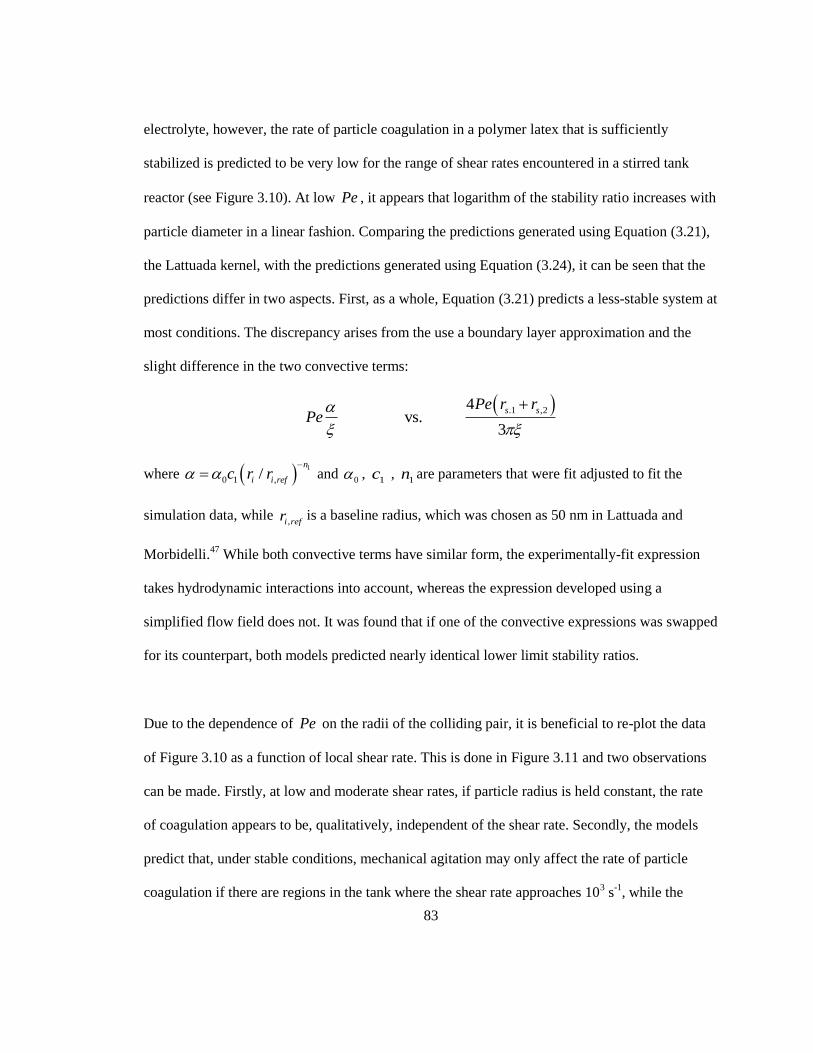
83
electrolyte, however, the rate of particle coagulation in a polymer latex that is sufficiently
stabilized is predicted to be very low for the range of shear rates encountered in a stirred tank
reactor (see Figure 3.10). At low Pe , it appears that logarithm of the stability ratio increases with
particle diameter in a linear fashion. Comparing the predictions generated using Equation (3.21),
the Lattuada kernel, with the predictions generated using Equation (3.24), it can be seen that the
predictions differ in two aspects. First, as a whole, Equation (3.21) predicts a less-stable system at
most conditions. The discrepancy arises from the use a boundary layer approximation and the
slight difference in the two convective terms:
.1 ,24 vs.
3
s sPe r rPe
where 1
0 1 ,/n
i i refc r r
and 0 ,
1c , 1n are parameters that were fit adjusted to fit the
simulation data, while ,i refr is a baseline radius, which was chosen as 50 nm in Lattuada and
Morbidelli.47
While both convective terms have similar form, the experimentally-fit expression
takes hydrodynamic interactions into account, whereas the expression developed using a
simplified flow field does not. It was found that if one of the convective expressions was swapped
for its counterpart, both models predicted nearly identical lower limit stability ratios.
Due to the dependence of Pe on the radii of the colliding pair, it is beneficial to re-plot the data
of Figure 3.10 as a function of local shear rate. This is done in Figure 3.11 and two observations
can be made. Firstly, at low and moderate shear rates, if particle radius is held constant, the rate
of coagulation appears to be, qualitatively, independent of the shear rate. Secondly, the models
predict that, under stable conditions, mechanical agitation may only affect the rate of particle
coagulation if there are regions in the tank where the shear rate approaches 103 s
-1, while the
84
maximum observed shear rate in the CFD simulations was on the order of 102 s
-1. Additional CFD
simulations using higher resolution grids are required in order to resolve the fine structure of the
trailing vortices and whether the maximum rate of shear surpasses 103 s
-1.
Figure 3.10. Dependency of the stability ratio on the local particle Peclet number for binary
collisions between equal-sized colloidal particles, as computed using Equations (3.21) and
(3.24). 𝛆 = 6.91 × 10⁻¹⁰
s2C
2m
-1kg
-1, T = 298 K, 𝛋 = 3.21×10
8 m
-1 and 𝛙 = 3.35×10
-2 V.
85
Figure 3.11. Dependency of the stability ratio on the local shear rate for binary collisions
between equal-sized colloidal particles, as computed using Equations (3.21) and (3.24).
𝛆 = 6.91 × 10⁻¹⁰
s2C
2m
-1kg
-1, T = 298 K, 𝛋 = 3.21×10
8 m
-1 and 𝛙 = 3.35×10
-2 V.
Controlled coagulation, where the polymer latex is purposefully coagulated using mechanical
and/or chemical means, is employed in the production of polymeric materials for powders,
coatings and cosmetics.114
The addition of electrolyte is predicted to change coagulation behavior,
as can be seen in Figure 3.12. The Lattuada model predicts that the smallest particles will
coagulate rapidlyfast , while the rate of shear in the impeller region may be high enough to
enhance the rate of coagulation of larger particles. As might be expected, the coagulation kernel
based on a simple velocity profile predicts, on a while, a much higher rate of particle coagulation
and a greater sensitivity to mechanical agitation. Recall from Figure 3.9 that both the Lattuada
model and the thorough numerical simulation data suggest that the compression of the
electrostatic double layer will reduce the latex‟s sensitivity to mechanical agitation; this is the
same effect that gives rise to the discrepancy between the model predictions in Figure 3.12.
While a coagulation kernel based on the Lattuada model would be challenging to implement
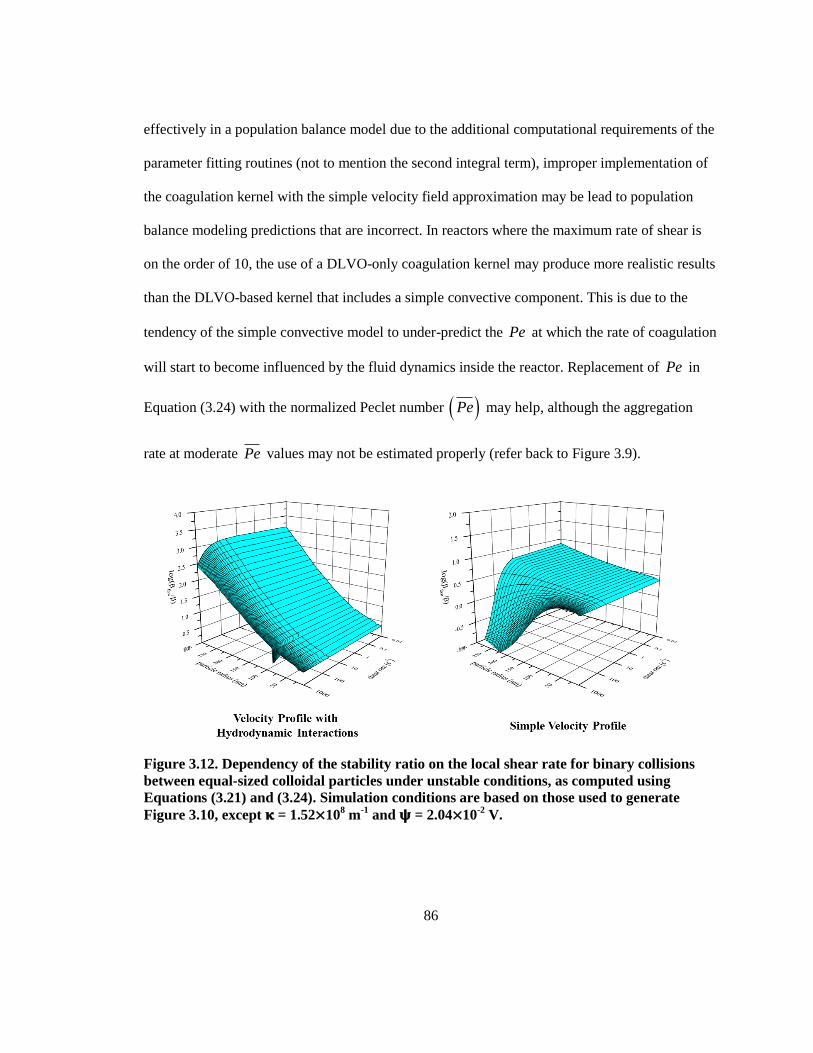
86
effectively in a population balance model due to the additional computational requirements of the
parameter fitting routines (not to mention the second integral term), improper implementation of
the coagulation kernel with the simple velocity field approximation may be lead to population
balance modeling predictions that are incorrect. In reactors where the maximum rate of shear is
on the order of 10, the use of a DLVO-only coagulation kernel may produce more realistic results
than the DLVO-based kernel that includes a simple convective component. This is due to the
tendency of the simple convective model to under-predict the Pe at which the rate of coagulation
will start to become influenced by the fluid dynamics inside the reactor. Replacement of Pe in
Equation (3.24) with the normalized Peclet number Pe may help, although the aggregation
rate at moderate Pe values may not be estimated properly (refer back to Figure 3.9).
Figure 3.12. Dependency of the stability ratio on the local shear rate for binary collisions
between equal-sized colloidal particles under unstable conditions, as computed using
Equations (3.21) and (3.24). Simulation conditions are based on those used to generate
Figure 3.10, except 𝛋 = 1.52×10⁸ m
-1 and 𝛙 = 2.04×10
-2 V.
87
3.5 Conclusions
Recent advances in the modeling of particle coagulation may potentially improve the
performance of existing population balance models, providing them with the functionality to
correctly estimate the rate of particle coagulation over a wide range of flow conditions. CFD
simulations suggested that the maximum shear rate and range of shear rates that the latex particles
are exposed to will change as the reactor is scaled-up and the flow regime changes from
transitional to fully-turbulent. Unexpectedly, the CFD simulations suggested that the maximum
rate of shear arising from the turbulent eddies will decrease rather than increase with reactor
scale. Further CFD simulation on higher resolution grids is likely necessary, in order to ensure the
behavior of the trailing vortices is being modeled accurately. Regardless, the shear field may
influence the rate of aggregation at all reactor scales, especially when the average latex particle
diameter is large and the double layer is diffuse due to a low disperse phase ionic strength. The
simple shear model, which was derived assuming a uniform velocity gradient at the microscopic
scale, does not match the predictions of the more thorough coagulation model that includes
adjustable parameters to account for additional hydrodynamic effects. The simple shear kernel is
likely to severely over-predict the contribution of the shear field in unstable conditions, such as
when a polymer latex is coagulated through the addition of an electrolyte. Therefore the use of a
DLVO-only coagulation kernel is preferable to the simple shear kernel when modeling the scale-
up of a controlled coagulation processes.
88
Chapter 4
Development of a Computational Framework to Model the Scale Up of
High Solid Content Polymer Latex Coagulators
4.1 Introduction
Synthetic polymer latex products, which are colloidally stable dispersions of nano-scale polymer
particles in a continuous medium, are an important class of synthetic materials. Polymer latex
products are used in a wide range of applications, including the production of bulk polymer,
paints, coatings, adhesives and carpet backing, with annual production exceeding 20 million
tonnes.1 Most industrial polymer latex formulations contain between 40 to 55 vol.-% solids, the
remainder being dissolved species and water. There is ongoing commercial interest in developing
high solid content latexes that contain as much as 75 vol.-% solids; this push toward higher solid
contents is motivated by potential cost savings in production and transportation, along with
improvements in the quality of the end-use product.30
However formulation of these dispersions
typically requires a well-defined particle size distribution (PSD) in order to maintain both
colloidal stability and an acceptable product viscosity.25
A number of recently-published results
have shown that it is possible to produce low viscosity latexes with solid loadings above 70 vol.-
% if the PSD is well-engineered;26, 27
typically, the target PSD will be broad and bimodal, with
the small particles designed to fit in the interstices created by the large particle lattice.
Commercial interest in driving up the solid content of existing recipes provides sufficient
motivation to adapt many of the novel production techniques outlined in the academic literature
89
to larger scale production. Careful attention must be paid to any changes in process-critical time
and length scales that may arise from changes in process scale. A survey of the academic
literature reveals that high solid content polymer latexes are typically produced by growing a
primary population of seed particles while simultaneously creating a secondary population of
smaller particles via homogeneous nucleation.30
Control over the PSD is achieved by adjusting
the feed rates and ratios of monomer, initiator and surfactant species. Particular attention needs
to be paid to the dispersion of ionic species as local variations in the ionic strength can have a
major impact on particle coagulation, and therefore the PSD and viscosity. At the laboratory scale
the impeller rotational speed can be increased to ensure that feed dispersion is instantaneous
relative to the rate of polymerization; such adjustments are physically and/or economically
unfeasible at the commercial scale. Concentrated polymer latexes will exhibit non-Newtonian
flow characteristics; in the laminar flow regime, this leads to segregation outside the impeller
zone and characteristic mixing times on the order of minutes.14
It is therefore of interest to
understand the relationship between the coagulation, reaction and mixing rates as the process is
scaled-up.
There are a number of general texts available that provide general guidelines for process scale-up,
including Tatterson,115
Oldshue10
and Kresta.116
The most popular scale-up approach is to assume
that geometric similarity can be maintained and that the mixing objectives can be met by
maintaining a constant power input per unit volume (a constant P/V ratio). In polymerization
processes, heat removal is often the limiting factor for reactor performance, necessitating an
increase in the tank height to tank diameter ratio. Neglecting the issue of heat transfer, the
classical heuristics are only a starting point and they provide no information regarding flow
90
patterns, mixing mechanisms and the degree of homogeneity inside the reaction vessel. Advanced
experimental methods such as Laser Doppler Velocimetry (LDV) and Particle Image Velocimetry
(PIV)117
can provide further insight, however these methods are unsuitable for studying flow in
industrial-scale vessels, where the vessels are made of non-transparent materials and the process
liquids are opaque.74
The availability of affordable high-performance computing hardware and experimentally-
validated process simulation software has led to the demand for process-specific models to assist
in the scale-up process. Due to myriad assumptions that are made during model development to
ensure reasonable calculation time(s), computational modeling does not eliminate the need for
pilot plant experimentation. Good predictive tools can, however reduce development lead times
and costs. In the production and processing of polymer latexes, the computational framework
must be designed with the goal of predicting changes in product quality that arise from changes in
production scale; in high solid content latexes, product quality is dependent on maintaining a
well-defined PSD. Over the past decade, significant progress has been made in the development
of mathematical models for predicting the evolution of PSD under different operating conditions.
The complex PSDs required to produce high solid content (HSC) latexes necessitate the use of
population balances for PSD prediction.8
Over the past two decades, computational fluid dynamics (CFD) has become a powerful tool in
the process industry, as CFD simulations are capable of imparting detailed insight regarding the
flow patterns, mixing mechanisms and degree of homogeneity within a reactor vessel. CFD
simulation has provided unique insight into a number of polymerization processes including bulk
polymerization118
and suspension polymerization.119
It is theoretically possible to incorporate the
91
population balances directly into the CFD code by defining additional conservation equations.78
In practice, directly integrating the population balances into the CFD simulation is impractical as
the resulting system of equations would be far too large to solve and process with current
computing equipment.
Given limited computational resources, the simplest way to couple the CFD simulation and
population balance models is to use them in a sequential manner. The hydrodynamics obtained
from CFD are used to identify a number of interacting spatial regions or zones, with each zone
being approximated as well-mixed; additionally the CFD is used to determine the rate of flow
exchanged between adjacent zones. The population balance models are then solved on this
coarser grid of interconnected zones. In many cases, it is expected that the hydrodynamics will
evolve significantly during the process, as the PSD changes (rheology is highly dependent on
PSD); this necessitates two-way coupling between CFD simulation and population balance
models. In a series of papers, Bezzo et al.78, 80, 81, 120
developed a generalized hybrid
multizonal/CFD modeling methodology to standardize the approach across a wide variety of
applications such as crystallization and bioreactor modeling.
The two compartment model framework developed by Alexopoulos et al. for liquid-liquid
dispersion in suspension polymerization83
and later emulsion polymerization15
represents one of
the first attempts to utilize the information provided by CFD to improve the predictive
capabilities of a polymerization process model, although the models are only coupled
sequentially. Elgebrandt et al.17
were the first group to adapt the general hybrid multizonal/CFD
framework to emulsion polymerization. Although they suggested that their framework could be
adapted to study the production of concentrated latexes, they limited the scope of their study to
92
operation in the turbulent regime and lower solid content latexes (a solid volume fraction of ~
25%) where latex rheology is Newtonian. The combined model relied on a 2D CFD mesh and an
essentially-qualitative coagulation kernel, leaving plenty of room for improvement. There has
been little follow-up since this work was published.
This chapter focuses on evaluating the feasibility of a hybrid multizonal/CFD model framework
to capture the dynamics of the final production stages of high solid content latexes, specifically
operation under conditions where fluid rheology is non-Newtonian and the reactor is operating in
the laminar or lower transition flow regimes. The hybrid model is employed to investigate the
impact of process scale-up on mixing performance in the controlled coagulation of concentrated
polymer latexes in the absence of chemical reaction in this initial step. Controlled coagulation is
employed in the production of polymeric materials for powders, coatings and cosmetics, but is
discussed very sparingly in the literature.114
The process model for controlled coagulation is
essentially a limited version of the process model for emulsion polymerization, ideal for
preliminary assessment of the framework‟s capabilities in this set of applications.
4.2 Overview of Framework Components
4.2.1 Mixing System
The mixing system consisted of a centered four-bladed 45° pitched blade turbine and two round
baffles. In order to investigate the impact of reactor scale-up, CFD simulations were run across
three (geometrically similar) reactor scales: 1 L, 10 L and 10 L, corresponding to tank diameters
(T) of 9.69 × 10⁻²
m, 2.09 × 10⁻¹
m and 4.50 × 10⁻¹
, respectively. As in Chapter 3, the liquid
93
level H was 1.4 times the tank diameter T and the impeller diameter was set to / 3T .
The remaining tank dimensions can be found on Figure 3.1 (Section 3.3) in Chapter 3. Although
baffles are not necessary for laminar mixing of viscous liquids, they are likely to be present in a
polymer latex reactor as they serve to eliminate vortex formation87
at early stages in the
polymerization when latex viscosity is low and flow is turbulent.
4.2.2 The Population Balance
Due to the fact that this paper is meant only as an overview and demonstration of the hybrid
multizonal/CFD framework, the current investigation is restricted to modeling controlled
coagulation. This eliminates the particle nucleation and particle growth via polymerization terms
from the population balance equation (PBE), but is still reflective of common polymerization
processes such as those outlined in Fortuny100
and Konstansek.114
The multizonal model is
comprised of a series of interconnected, well-mixed zones, thus eliminating the need to define an
external coordinate domain. The particle population is described using with the number density
function, ( , )f v t , such that ( , )f v t dv is the number of particles (per unit volume) with a volume
between v and v dv . The total number concentration of particles in the system can be
calculated by integrating the number density function over the entire size range of particles found
in the latex
min
( , )Pv
N f v t dV
(4.1)
In the case where coagulation is the only mechanism of particle creation and destruction, the total
mass of particles in the system will remain constant. Under the assumption that all coagulation
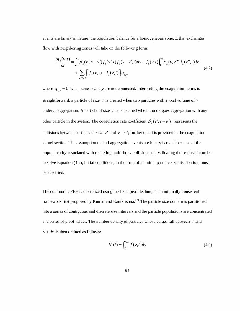
94
events are binary in nature, the population balance for a homogeneous zone, z, that exchanges
flow with neighboring zones will take on the following form:
0 0
,
,
( , )( ', ') ( ', ) ( ', ) ( , ) ( , ") ( ", )
( , ) ( , )
vz
z z z z z z
y z z y
y y z
df v tv v v f v t f v v t dv f v t v v f v t dv
dt
f v t f v t q
(4.2)
where , 0z yq when zones z and y are not connected. Interpreting the coagulation terms is
straightforward: a particle of size v is created when two particles with a total volume of v
undergo aggregation. A particle of size v is consumed when it undergoes aggregation with any
other particle in the system. The coagulation rate coefficient, ( ', ')z v v v , represents the
collisions between particles of size 'v and 'v v ; further detail is provided in the coagulation
kernel section. The assumption that all aggregation events are binary is made because of the
impracticality associated with modeling multi-body collisions and validating the results.8 In order
to solve Equation (4.2), initial conditions, in the form of an initial particle size distribution, must
be specified.
The continuous PBE is discretized using the fixed pivot technique, an internally-consistent
framework first proposed by Kumar and Ramkrishna.121
The particle size domain is partitioned
into a series of contiguous and discrete size intervals and the particle populations are concentrated
at a series of pivot values. The number density of particles whose values fall between v and
v dv is then defined as follows:
1
( ) ( , )i
i
v
iv
N t f v t dv
(4.3)
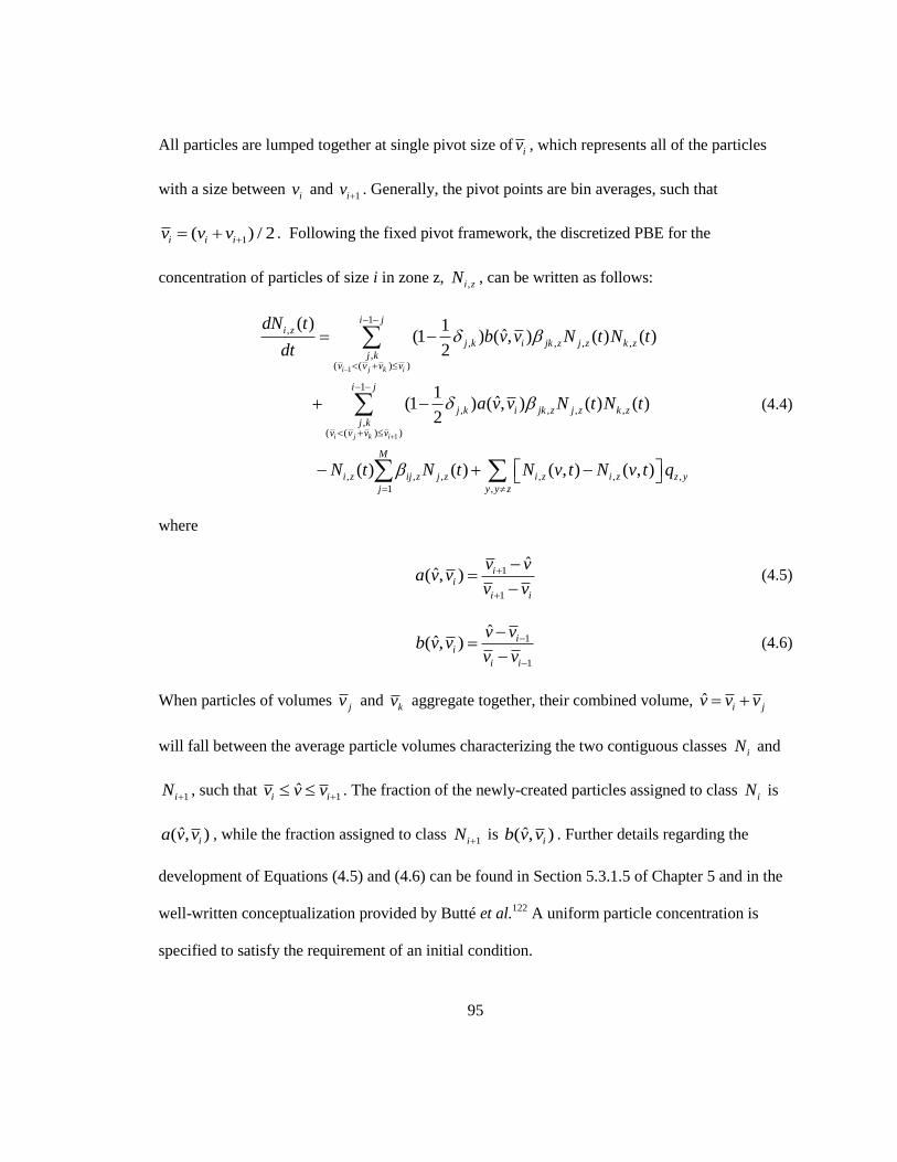
95
All particles are lumped together at single pivot size ofiv , which represents all of the particles
with a size between iv and
1iv . Generally, the pivot points are bin averages, such that
1( ) / 2i i iv v v . Following the fixed pivot framework, the discretized PBE for the
concentration of particles of size i in zone z, ,i zN , can be written as follows:
1
1
1,
, , , ,
,( ( ) )
1
, , , ,
,( ( ) )
, , , , ,
1
( ) 1ˆ(1 ) ( , ) ( ) ( )
2
1ˆ(1 ) ( , ) ( ) ( )
2
( ) ( ) ( , )
i j k i
i j k i
i ji z
j k i jk z j z k z
j kv v v v
i j
j k i jk z j z k z
j kv v v v
M
i z ij z j z i z i
j
dN tb v v N t N t
dt
a v v N t N t
N t N t N v t N
,
,
( , )z z y
y y z
v t q
(4.4)
where
1
1
ˆˆ( , ) i
i
i i
v va v v
v v
(4.5)
1
1
ˆˆ( , ) i
i
i i
v vb v v
v v
(4.6)
When particles of volumes jv and
kv aggregate together, their combined volume, ˆi jv v v
will fall between the average particle volumes characterizing the two contiguous classes iN and
1iN , such that
1ˆ
i iv v v . The fraction of the newly-created particles assigned to class iN is
ˆ( , )ia v v , while the fraction assigned to class 1iN is ˆ( , )ib v v . Further details regarding the
development of Equations (4.5) and (4.6) can be found in Section 5.3.1.5 of Chapter 5 and in the
well-written conceptualization provided by Butté et al.122
A uniform particle concentration is
specified to satisfy the requirement of an initial condition.
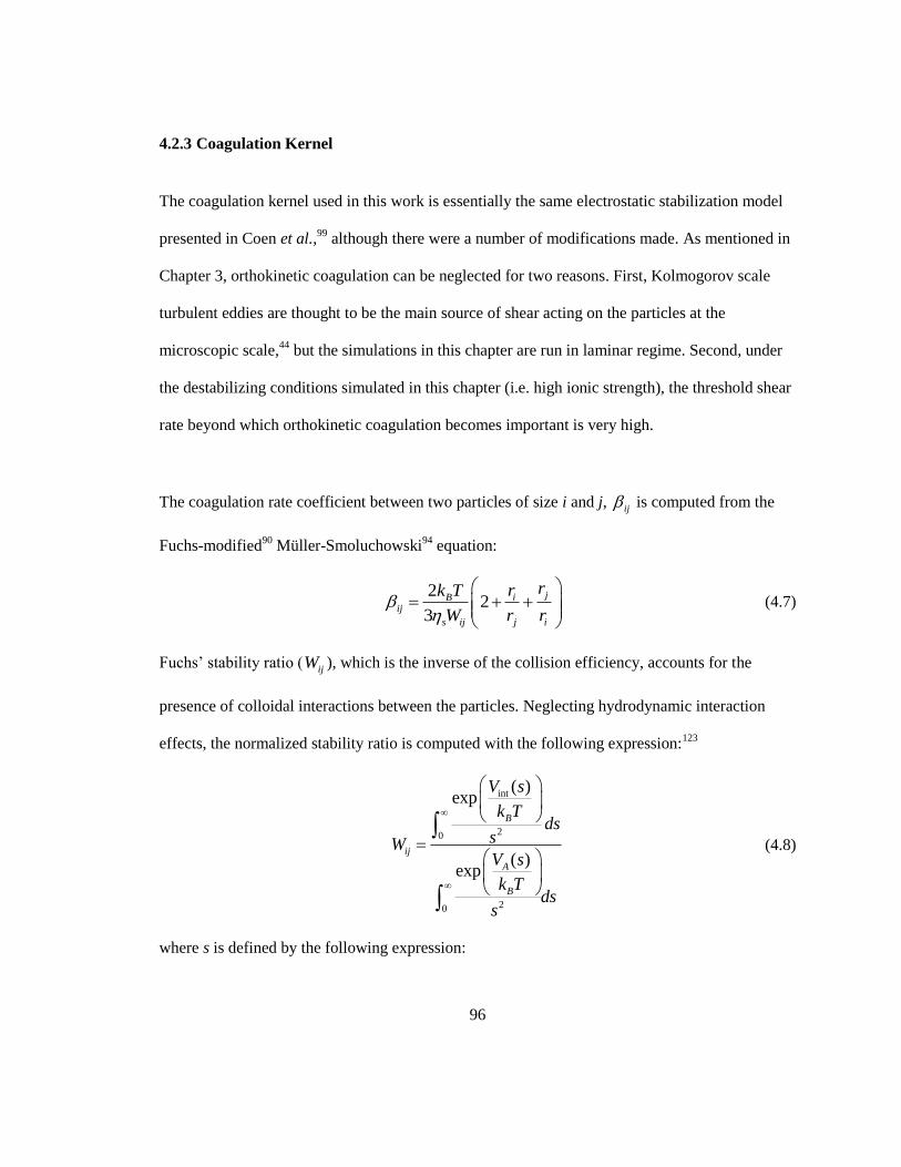
96
4.2.3 Coagulation Kernel
The coagulation kernel used in this work is essentially the same electrostatic stabilization model
presented in Coen et al.,99
although there were a number of modifications made. As mentioned in
Chapter 3, orthokinetic coagulation can be neglected for two reasons. First, Kolmogorov scale
turbulent eddies are thought to be the main source of shear acting on the particles at the
microscopic scale,44
but the simulations in this chapter are run in laminar regime. Second, under
the destabilizing conditions simulated in this chapter (i.e. high ionic strength), the threshold shear
rate beyond which orthokinetic coagulation becomes important is very high.
The coagulation rate coefficient between two particles of size i and j, ij is computed from the
Fuchs-modified90
Müller-Smoluchowski94
equation:
2
2 3
jiBij
s ij j i
rrk T
W r r
(4.7)
Fuchs‟ stability ratio (ijW ), which is the inverse of the collision efficiency, accounts for the
presence of colloidal interactions between the particles. Neglecting hydrodynamic interaction
effects, the normalized stability ratio is computed with the following expression:123
int
20
20
( )exp
( )exp
B
ij
A
B
V s
k Tds
sWV s
k Tds
s
(4.8)
where s is defined by the following expression:
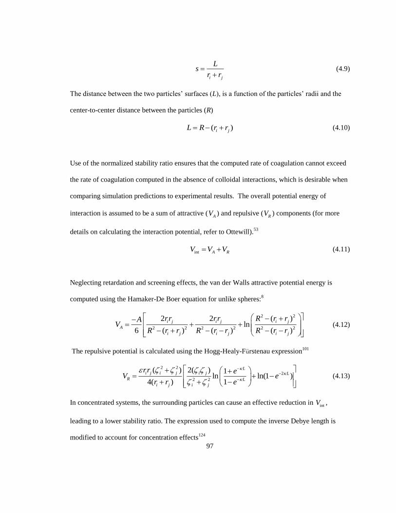
97
i j
Ls
r r
(4.9)
The distance between the two particles‟ surfaces (L), is a function of the particles‟ radii and the
center-to-center distance between the particles (R)
( )i jL R r r (4.10)
Use of the normalized stability ratio ensures that the computed rate of coagulation cannot exceed
the rate of coagulation computed in the absence of colloidal interactions, which is desirable when
comparing simulation predictions to experimental results. The overall potential energy of
interaction is assumed to be a sum of attractive (AV ) and repulsive (
RV ) components (for more
details on calculating the interaction potential, refer to Ottewill).53
int A RV V V (4.11)
Neglecting retardation and screening effects, the van der Walls attractive potential energy is
computed using the Hamaker-De Boer equation for unlike spheres:8
2 2
2 2 2 2 2 2
2 2 ( )ln
6 ( ) ( ) ( )
i j i j i j
A
i j i j i j
rr rr R r rAV
R r r R r r R r r
(4.12)
The repulsive potential is calculated using the Hogg-Healy-Fürstenau expression101
2 2
2
2 2
( ) 2( ) 1ln ln(1 )
4( ) 1
Li j i j i j L
R L
i j i j
rr eV e
r r e
(4.13)
In concentrated systems, the surrounding particles can cause an effective reduction in intV ,
leading to a lower stability ratio. The expression used to compute the inverse Debye length is
modified to account for concentration effects124
98
2 24
1
totA
B
AN I
e e
k T
(4.14)
The expression /totA e accounts for the counterions carried by neighboring particles, while the
denominator of 1 accounts for the reduced solution volume available to ions. The ionic
strength of the solution (I) is defined as
[ ] [ ]I S E (4.15)
while the permittivity of water is defined in CGS units by multiplying the relative
permittivity r by the permittivity of free space 0 :
04 r (4.16)
For a discrete population of particles, the total surface area of the latex particles is computed as
follows:
2
1
4 ( )m
tot i i
i
A n r r
(4.17)
In the absence of initiator, the surface charge on each particle is dictated by the adsorption of
surfactant onto the particle surface
s
z e
A (4.18)
where the counter-ion valence z is equal to one for an initiator such as potassium
persulphate. The area occupied by a surfactant molecule sA is dependent on the partitioning of
added surfactant between the aqueous phase and the surface of the latex particles which follows
the Langmuir adsorption isotherm:99
99
11s s
sw
A aS b
(4.19)
The concentration of surfactant in the aqueous phase wS is dependent on the concentration of
surfactant added in the continuous phase S and the total amount of surfactant adsorbed onto
the particles‟ surfaces
[ ] [ ] totw
A s
AS S
N A (4.20)
Combining Equations (4.19) and (4.20) and solving for the positive root yields the relationship
used to compute wS .
2
1 4[ ][ ]
1[ ]
2
tot
s A s stot
ws A s
A SS
a N b bAS S
a N b
(4.21)
Finally, the surface potential and zeta potential are calculated following the approach used by
Coen et al.99
The surface potential is calculated from the surface charge density using one of the
two following relationships (valid for 25 mV ) :
4
= for 1(1 )
s
s
rr
r
(4.22)
12 2
sinh for 1B
B
k T er
e k T
(4.23)
If 1r , the curvature of the particle surface must be taken into account, as shown in Equation
(4.22); however, if 1r , the surface can be approximated as a flat plate and Equation (4.23) is
used instead. The zeta potential is computed with the following expressions:
100
4
4
2 exp( ) 1ln
exp( ) 1
Bk T
z e
(4.24)
54
5
exp( ) 1ln
exp( ) 1
(4.25)
52 B
z e
k T
(4.26)
It must be noted that Equations (4.22) and (4.23) are derived assuming a Boltzmann distribution
of electrostatic potential at the particle surface; this is not the case since the ions do not move
freely at the surface.
4.2.4 CFD Model
Due to the presence of baffles within the tank, the flow field within the tank may be unsteady in
nature, requiring a non-steady-state simulation when operating in turbulent conditions. This is not
necessarily the case in the laminar and lower transition regime, so a preliminary set of CFD
simulations were run to evaluate the degree of unsteadiness in the flow field. The non-stationary
flow field, generated using the fictitious domain method to handle impeller rotation, was
compared to the stationary flow field generated using a rotational boundary condition on the
impeller surface. It was found that the shape of the non-stationary flow field remained
qualitatively constant regardless of impeller position and the variation in the computed power
consumption during a period of rotation was less 10%. Given that the framework architecture
requires that the flow field be re-computed each time the properties of the liquid change
significantly, a decision was made to switch to a steady-state CFD model in order to reduce total
computation times from the scale of days to hours
101
The flow field was predicted by solving the momentum and continuity equations with a standard
3D Galerkin finite element method. Fluid density and temperature are assumed to be constant. In
the absence of polymerization, the assumption of isothermal operation is reasonable.
2pt
vv v (4.27)
0 v (4.28)
The boundary conditions were as follows:
- Constant angular velocity along the impeller surface (NI = const)
- No slip condition at the baffles and along the vessel wall (v = 0)
- No normal velocity at the fluid surface which is assumed to be flat (vz = 0)
The 3D unstructured CFD mesh was generated with GAMBIT (Ansys), commercial CFD pre-
processing software. The mesh was refined near the impeller region and at the baffle walls in
order to provide sufficient resolution in regions with large velocity gradients (this was verified by
refining the mesh until the computed power consumption converged). The details of the mesh are
shown in Figure 4.1, using a vertical slice to cut through the center of the vessel. MINI finite
elements were used to approximate the velocity and pressure fields, as this element type has been
shown to be accurate and very computationally efficient relative to other element types.125
The
resulting computational mesh consisted of approximately 240,000 elements and 285,000 nodes,
resulting in a system of 150,000 equations. The non-linearity imposed by the non-Newtonian
rheological model was handled using an augmented Lagrangian approach in which the
rheological non-linearity is removed from the momentum equation and handled separately with
an auxiliary equation, yielding a Lagrange multiplier. A fully-coupled approach was used in
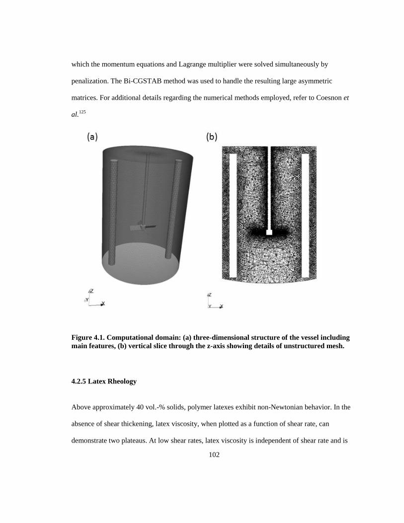
102
which the momentum equations and Lagrange multiplier were solved simultaneously by
penalization. The Bi-CGSTAB method was used to handle the resulting large asymmetric
matrices. For additional details regarding the numerical methods employed, refer to Coesnon et
al.125
Figure 4.1. Computational domain: (a) three-dimensional structure of the vessel including
main features, (b) vertical slice through the z-axis showing details of unstructured mesh.
4.2.5 Latex Rheology
Above approximately 40 vol.-% solids, polymer latexes exhibit non-Newtonian behavior. In the
absence of shear thickening, latex viscosity, when plotted as a function of shear rate, can
demonstrate two plateaus. At low shear rates, latex viscosity is independent of shear rate and is
103
said to obey Newtonian behavior. This lower plateau is referred to as the lower Newtonian
viscosity. At a certain shear rate (characteristic of the latex), the shear stress transmitted through
the aqueous medium will begin orienting the particles in the direction of flow. These layered
particles offer less resistance to flow, hence a lowering of the viscosity. Once the particles are
completely layered, viscosity can no longer decrease with increasing shear rate and this upper
plateau is referred to as the upper Newtonian viscosity. If shear rate is increased further, the mean
flow may impart enough energy to the particles so that they overcome the forces of repulsion and
begin clustering together. This clustering (not to be confused with coagulation) will disrupt the
layered flow which results in a large increase in latex viscosity. This clustering phenomenon,
known as shear thickening, may also result in coagulation which will exacerbate the increase in
viscosity. The phenomenon of shear thickening is not accounted for in this study, but care should
be taken to ensure that the maximum shear rate in the vessel does not approach the thickening
limit which is deleterious to the health of mixing equipment.54
The non-Newtonian rheology was
modeled with the Carreau-Yasuda model, which has been shown to correctly capture the shearing
behavior of concentrated latexes.5 The equations employed are the same as those employed in
Chapter 3. For further details, refer to Equations (3.27) to (3.29) and Table 3.1 in Section 3.3.
The maximum packing fraction of a polymer latex made up of m discrete particle sizes can be
calculated using a model proposed by Pishvaei et al.65
The advantage of this model is that it
eliminates the need for experimental data beyond the determination of the effective maximum
packing fractions ,m i and the PSD. For a system with m discretized particles sizes:
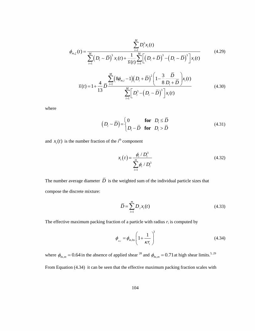
104
3
1,
3 3 3
1 1
( )
( )1
( ) ( )( )
M
i i
im M M
i i i i i
i i
D x t
t
D D x t D D D D x ts t
(4.29)
2
,
1
33
1
38 1 1 ( )
84( ) 1
13( )
M
m i i i
i i
M
i i i
i
DD D x t
D Ds t D
D D D x t
(4.30)
where
0 i
i
i i
D DD D
D D D D
for
for (4.31)
and ( )ix t is the number fraction of the ith component
3
3
1
/
/
i ii m
i i
i
Dx t
D
(4.32)
The number average diameter D is the weighted sum of the individual particle sizes that
compose the discrete mixture:
1
( )m
i i
i
D D x t
(4.33)
The effective maximum packing fraction of a particle with radius ri is computed by
,
3
,
11
m i m hs
ir
(4.34)
where , 0.64hs m in the absence of applied shear
28 and
, 0.71hs m at high shear limits.5, 29
From Equation (4.34) it can be seen that the effective maximum packing fraction scales with
105
particle size, approaching the hard sphere value at the limit. For further details, refer to Section
2.2.4 in Chapter 2.
Pishvaei demonstrated that Equations (4.29) through (4.33) provide reasonable estimates of the
loading limits for bimodal systems based on estimates of these properties from related
monodisperse latexes.65
In this work, the model is extended to work with multimodal PSDs in
which the distributions are broader. The continuous PSDs encountered in experimental work can
be approximated in the discretized form if the population balance mesh is sufficiently refined (m
~ 100).
4.3 Framework Overview
The computational framework comprised three components: the multizonal population balance
model, the CFD model and the interface that handles the transmission of data between the
models. The computational fluid simulations were performed on fine mesh, while the population
balance model was solved on a much coarser grid. The manner in which the three components
work together is schematically depicted in Figure 4.2.
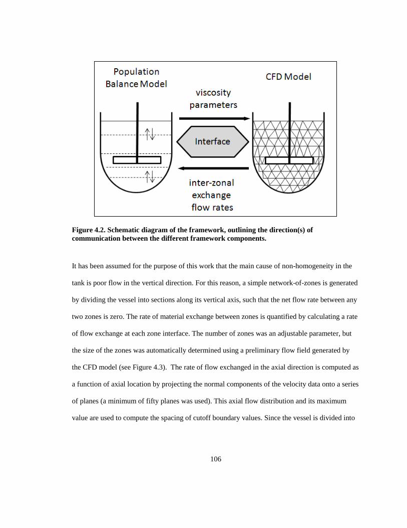
106
Figure 4.2. Schematic diagram of the framework, outlining the direction(s) of
communication between the different framework components.
It has been assumed for the purpose of this work that the main cause of non-homogeneity in the
tank is poor flow in the vertical direction. For this reason, a simple network-of-zones is generated
by dividing the vessel into sections along its vertical axis, such that the net flow rate between any
two zones is zero. The rate of material exchange between zones is quantified by calculating a rate
of flow exchange at each zone interface. The number of zones was an adjustable parameter, but
the size of the zones was automatically determined using a preliminary flow field generated by
the CFD model (see Figure 4.3). The rate of flow exchanged in the axial direction is computed as
a function of axial location by projecting the normal components of the velocity data onto a series
of planes (a minimum of fifty planes was used). This axial flow distribution and its maximum
value are used to compute the spacing of cutoff boundary values. Since the vessel is divided into
107
an equal number of zones above and below the well-mixed impeller region, the number of cutoff
boundary values required can be computed as follows:
12
zonescutoff
nn (4.35)
The zone boundaries were set using the normalized distribution of axial flow. At all reactor scales
simulated, it was found that the absolute maximum rate of axial flow exchange,
10 ,maxlog / 0.0L LF F , is located slightly above the impeller, but there is a second local
maximum at 10 ,maxlog / 0.15L LF F located slightly below the center of the impeller,
which is marked by a local maximum 10 ,maxlog / 0.75L LF F . It was found that the
numerical solution was unstable (i.e. the solution did not converge as the number of zones was
increased) if the center zone did not enclose both maxima. Enclosure was ensured by locating the
center zone boundaries where 10 ,maxlog / 0.75L LF F drops just below this local
minimum, as illustrated in Figure 4.3 . Note that the normalized value of the local minimum was
found to be independent of the reactor scale. The outermost zones corresponded to regions where
mixing was poor and the normalized rate of axial flow exchange was low. From preliminary
simulation data it was determined that the solution did not change as long as the outer boundaries
were located at 10 ,maxlog / 2.0L LF F . Since the location of the outer and inner zone
boundaries are specified, a minimum of five zones was specified. If more than five zones are
desired, additional cutoff values are generated at equally spaced intervals between the two
extrema (-0.75 and -2.0). For example, for seven zones, the three cutoff values used to locate and
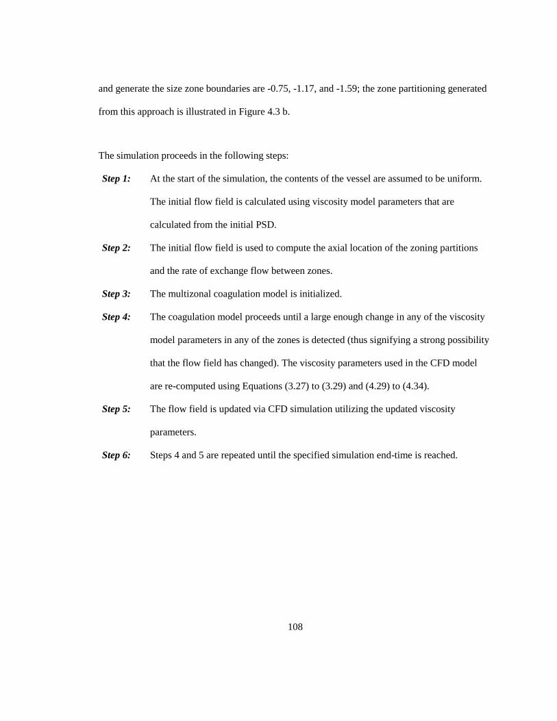
108
and generate the size zone boundaries are -0.75, -1.17, and -1.59; the zone partitioning generated
from this approach is illustrated in Figure 4.3 b.
The simulation proceeds in the following steps:
Step 1: At the start of the simulation, the contents of the vessel are assumed to be uniform.
The initial flow field is calculated using viscosity model parameters that are
calculated from the initial PSD.
Step 2: The initial flow field is used to compute the axial location of the zoning partitions
and the rate of exchange flow between zones.
Step 3: The multizonal coagulation model is initialized.
Step 4: The coagulation model proceeds until a large enough change in any of the viscosity
model parameters in any of the zones is detected (thus signifying a strong possibility
that the flow field has changed). The viscosity parameters used in the CFD model
are re-computed using Equations (3.27) to (3.29) and (4.29) to (4.34).
Step 5: The flow field is updated via CFD simulation utilizing the updated viscosity
parameters.
Step 6: Steps 4 and 5 are repeated until the specified simulation end-time is reached.
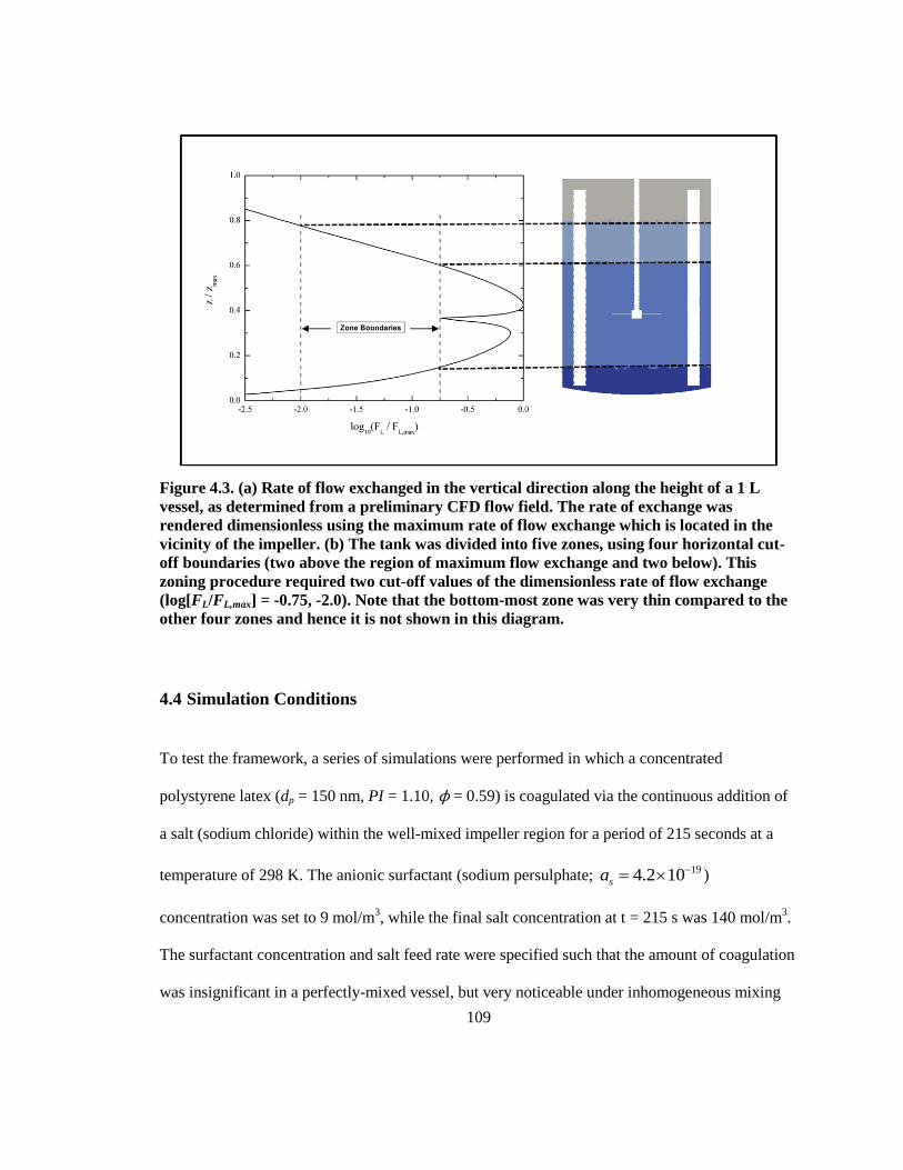
109
Figure 4.3. (a) Rate of flow exchanged in the vertical direction along the height of a 1 L
vessel, as determined from a preliminary CFD flow field. The rate of exchange was
rendered dimensionless using the maximum rate of flow exchange which is located in the
vicinity of the impeller. (b) The tank was divided into five zones, using four horizontal cut-
off boundaries (two above the region of maximum flow exchange and two below). This
zoning procedure required two cut-off values of the dimensionless rate of flow exchange
(log[FL/FL,max] = -0.75, -2.0). Note that the bottom-most zone was very thin compared to the
other four zones and hence it is not shown in this diagram.
4.4 Simulation Conditions
To test the framework, a series of simulations were performed in which a concentrated
polystyrene latex (dp = 150 nm, PI = 1.10, ϕ = 0.59) is coagulated via the continuous addition of
a salt (sodium chloride) within the well-mixed impeller region for a period of 215 seconds at a
temperature of 298 K. The anionic surfactant (sodium persulphate; 194.2 10sa )
concentration was set to 9 mol/m3, while the final salt concentration at t = 215 s was 140 mol/m
3.
The surfactant concentration and salt feed rate were specified such that the amount of coagulation
was insignificant in a perfectly-mixed vessel, but very noticeable under inhomogeneous mixing
110
when local salt concentration would approach and exceed critical coagulation concentration and
collision efficiency approaches 100 % (i.e. fast and the rate of coagulation is governed by
Brownian motion).
All CFD simulations were run using POLY3D (Rheosoft Inc.), a commercial 3D finite element
code using the numerical techniques described earlier in the paper. Post-Processing was carried
out using customized FORTRAN routines and Paraview (Kitware). Based on the objective of
maintaining a constant volumetric power input, the impeller rotational speed must be lowered
when the vessel is scaled-up, based on the following relationships:87
3 2
I I
PN D
V (4.36)
2
3,1
,2 ,1
,2
I
I I
I
DN N
D
(4.37)
Based on this scale-up approach, when reactor volume is increased by a factor of ten, the impeller
rotational rate should be multiplied by a factor of approximately 0.60.
The population balance model was coded in FORTRAN. The solution for the resulting system of
ODEs was computed with DLSODE, a general-purpose, open source, multi-step explicit
numerical scheme. DLSODE uses a multi-step backward differentiation formula (BDF) when
presented with stiff problems.126
The integral term contained within the coagulation kernel was
evaluated using a simple composite midpoint method. Coagulation rate coefficients were re-
calculated only when there was a change in any of the parameters that governed the rate of
particle coagulation. The number of pivot points was varied between 20 and 200; it was found
111
that mesh size of 100 pivot points (per zone) provided a grid-independent solution. All of the
simulation results presented in this work were run on an Intel Core 2 Quad Q6600 (2.4 GHz)
desktop computer. In order to determine the number of subdivisions required to obtain a solution
that is independent of the number of zones specified, a series of simulations were run in which the
number of zones was varied from five to eleven in odd increments. Examining the end-time PSDs
under various conditions, it was determined that dividing the reactor into nine zones was
sufficient to ensure the solution was not grid dependent under the current zoning scheme. For a
nine-zone system complete simulation times ranged from approximately 45 minutes to 90
minutes depending on the operational regime in the CFD simulations (laminar or transition), and
the frequency with which the flow field required updating. The frequency at which the flow field
was updated was adjusted by setting the tolerance of relative change in the PSD-dependent
viscosity parameters to ensure the final PSDs were independent of the update frequency.
4.5 Results & Discussion
One of the key changes made to the coagulation kernel when it was adapted from the works of
Coen et al.99
and Fortuny et al 100
was the modification of the expression used to calculate the
inverse Debye length to incorporate a particle concentration effect. Equation (4.14) indicates that,
for constant surface coverage conditions, an increase in solids content will lead to a reduction in
the thickness of the Debye length. Therefore the thickness of the double layer surrounding the
particles is reduced as the solids volume fraction is increased, which allows the particles to pack
closer together before repulsive forces become too great. The modified expression has two
effects; in addition to the obvious reduction in latex stability with increasing solid content, the
rheological behavior of the latex is affected as well. The reduction in the thickness of the double
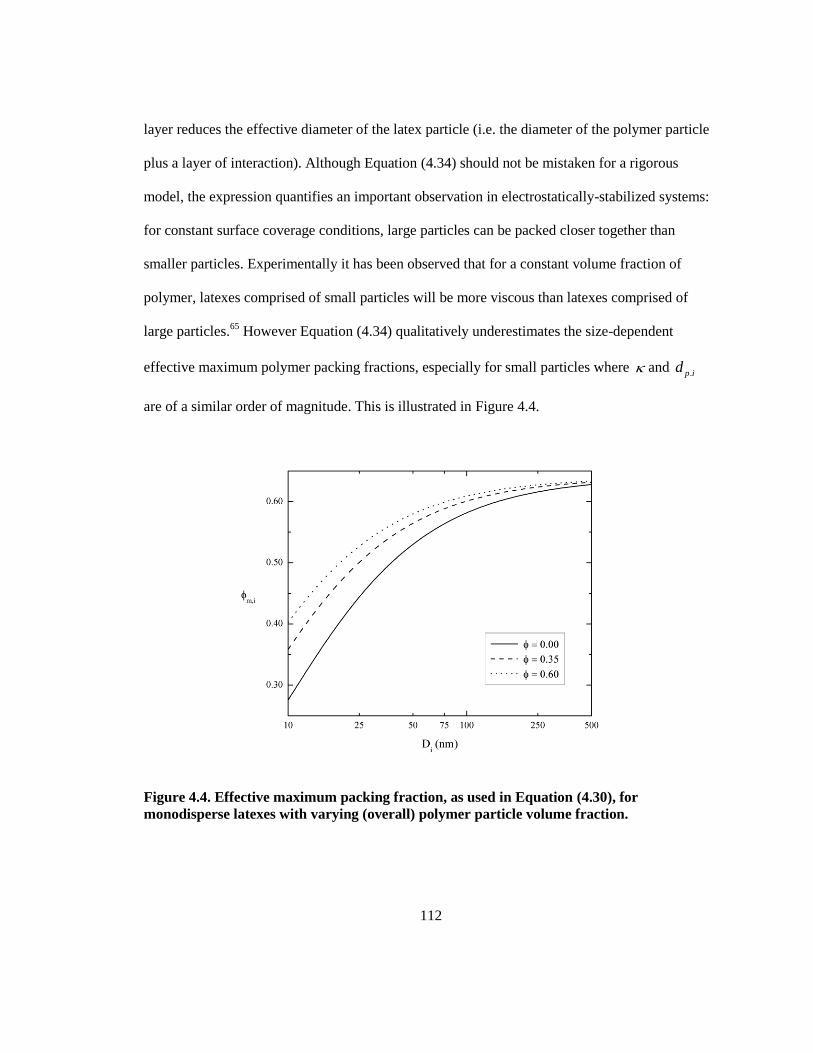
112
layer reduces the effective diameter of the latex particle (i.e. the diameter of the polymer particle
plus a layer of interaction). Although Equation (4.34) should not be mistaken for a rigorous
model, the expression quantifies an important observation in electrostatically-stabilized systems:
for constant surface coverage conditions, large particles can be packed closer together than
smaller particles. Experimentally it has been observed that for a constant volume fraction of
polymer, latexes comprised of small particles will be more viscous than latexes comprised of
large particles.65
However Equation (4.34) qualitatively underestimates the size-dependent
effective maximum polymer packing fractions, especially for small particles where and .p id
are of a similar order of magnitude. This is illustrated in Figure 4.4.
Figure 4.4. Effective maximum packing fraction, as used in Equation (4.30), for
monodisperse latexes with varying (overall) polymer particle volume fraction.
113
Conceptually, if one was to take a monodisperse latex and increase the solids concentration, the
increase in inter-particle interactions would continually push the maximum solids concentration
upwards until ,m i . It can be seen from Equation (3.28) in Chapter 3 that the key rheological
parameters are functions of and ,m i , so the rheological model behavior will be slightly
different as a result (viscosity predictions will be lower).
To estimate the tank Reynolds number for a Carreau-Yasuda fluid, it was assumed that the
infinite shear viscosity can be used to ascertain the most probable mixing regime inside the
vessel. Preliminary simulation results indicated that the shear rates within the impeller region are
sufficiently high that latex viscosity in this region can be approximated by the infinite shear
viscosity. At the very least, the mixing Reynolds number calculated using the infinite shear
viscosity can serve as an upper bound when designing mixing systems for high solid content
latexes, although recent studies suggest that the onset of turbulence in non-Newtonian fluids is
somewhat delayed compared to Newtonian fluids.109
The mixing Reynolds number is defined as
2
Re I IN D
(4.38)
Scaling the reactor volume by a factor of ten will result in a scaling in reactor diameter by factor
of approximately 2.15, provided geometric similarity is maintained. As stated prior, impeller
rotational speed is reduced by a factor of 0.6, so it can be ascertained from Equation (4.38) that
the Reynolds number will scale by a factor of approximately 2.75. As a general guideline, a tank
Reynolds number of 100 is considered the approximate cut-off between laminar and transition
flow, although the point at which inertial forces become important can vary significantly for
different mixing configurations and fluid types.
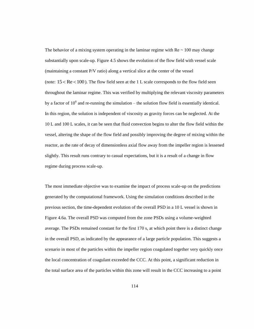
114
The behavior of a mixing system operating in the laminar regime with Re ~ 100 may change
substantially upon scale-up. Figure 4.5 shows the evolution of the flow field with vessel scale
(maintaining a constant P/V ratio) along a vertical slice at the center of the vessel
(note: 15 Re 100 ). The flow field seen at the 1 L scale corresponds to the flow field seen
throughout the laminar regime. This was verified by multiplying the relevant viscosity parameters
by a factor of 106 and re-running the simulation – the solution flow field is essentially identical.
In this region, the solution is independent of viscosity as gravity forces can be neglected. At the
10 L and 100 L scales, it can be seen that fluid convection begins to alter the flow field within the
vessel, altering the shape of the flow field and possibly improving the degree of mixing within the
reactor, as the rate of decay of dimensionless axial flow away from the impeller region is lessened
slightly. This result runs contrary to casual expectations, but it is a result of a change in flow
regime during process scale-up.
The most immediate objective was to examine the impact of process scale-up on the predictions
generated by the computational framework. Using the simulation conditions described in the
previous section, the time-dependent evolution of the overall PSD in a 10 L vessel is shown in
Figure 4.6a. The overall PSD was computed from the zone PSDs using a volume-weighted
average. The PSDs remained constant for the first 170 s, at which point there is a distinct change
in the overall PSD, as indicated by the appearance of a large particle population. This suggests a
scenario in most of the particles within the impeller region coagulated together very quickly once
the local concentration of coagulant exceeded the CCC. At this point, a significant reduction in
the total surface area of the particles within this zone will result in the CCC increasing to a point
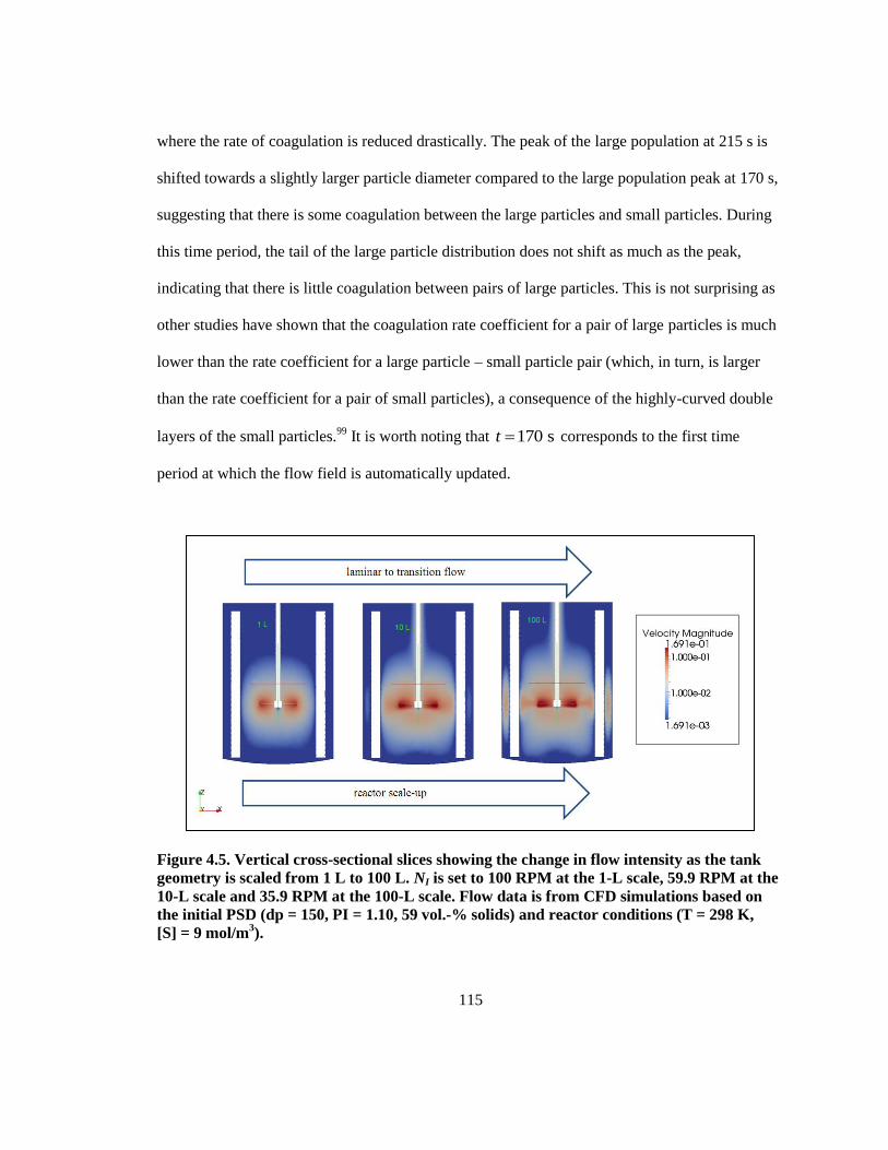
115
where the rate of coagulation is reduced drastically. The peak of the large population at 215 s is
shifted towards a slightly larger particle diameter compared to the large population peak at 170 s,
suggesting that there is some coagulation between the large particles and small particles. During
this time period, the tail of the large particle distribution does not shift as much as the peak,
indicating that there is little coagulation between pairs of large particles. This is not surprising as
other studies have shown that the coagulation rate coefficient for a pair of large particles is much
lower than the rate coefficient for a large particle – small particle pair (which, in turn, is larger
than the rate coefficient for a pair of small particles), a consequence of the highly-curved double
layers of the small particles.99
It is worth noting that 170 st corresponds to the first time
period at which the flow field is automatically updated.
Figure 4.5. Vertical cross-sectional slices showing the change in flow intensity as the tank
geometry is scaled from 1 L to 100 L. NI is set to 100 RPM at the 1-L scale, 59.9 RPM at the
10-L scale and 35.9 RPM at the 100-L scale. Flow data is from CFD simulations based on
the initial PSD (dp = 150, PI = 1.10, 59 vol.-% solids) and reactor conditions (T = 298 K,
[S] = 9 mol/m3).
116
An assessment of the zone-by-zone PSDs after 215 s (see Figure 4.6b) suggests that, regardless of
changes in the hydrodynamics due to a significant reduction in viscosity within the impeller
region, there is significant segregation outside the impeller region of the vessel. None of the small
particles contained within the uppermost region (zone 9) coagulated, while essentially all of the
particles in the impeller region (zone 5) coagulated together to form large particles. The presence
of a tiny peak of small particles seen in zone 5 is likely a result of ongoing exchange with the
zones immediately above and below it (zones 4 & 6). Comparing this tiny peak with the relatively
larger peak of large particles seen in zone 7 suggests that small particles entering the well-mixed
impeller region are quickly consumed via coagulation with themselves and with larger particles.
Such information regarding spatial variations in PSD is often impossible to obtain
experimentally, particularly inside commercial vessels where sampling is likely to be done in one
region only. Given the system dynamics, the topmost and bottommost zones can be treated as
completely segregated if the timescale of the coagulation process is in the order of seconds.
However the simulation results suggest that if the feed of coagulant is terminated and the contents
of the vessel are allowed to mix for a period of hours, the spatial variation in PSD will eventually
disappear.
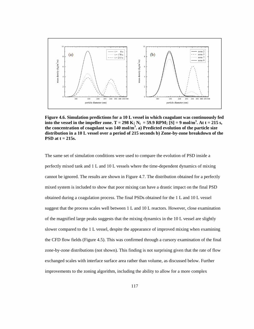
117
Figure 4.6. Simulation predictions for a 10 L vessel in which coagulant was continuously fed
into the vessel in the impeller zone. T = 298 K; NI = 59.9 RPM; [S] = 9 mol/m3. At t = 215 s,
the concentration of coagulant was 140 mol/m3. a) Predicted evolution of the particle size
distribution in a 10 L vessel over a period of 215 seconds b) Zone-by-zone breakdown of the
PSD at t = 215s.
The same set of simulation conditions were used to compare the evolution of PSD inside a
perfectly mixed tank and 1 L and 10 L vessels where the time-dependent dynamics of mixing
cannot be ignored. The results are shown in Figure 4.7. The distribution obtained for a perfectly
mixed system is included to show that poor mixing can have a drastic impact on the final PSD
obtained during a coagulation process. The final PSDs obtained for the 1 L and 10 L vessel
suggest that the process scales well between 1 L and 10 L reactors. However, close examination
of the magnified large peaks suggests that the mixing dynamics in the 10 L vessel are slightly
slower compared to the 1 L vessel, despite the appearance of improved mixing when examining
the CFD flow fields (Figure 4.5). This was confirmed through a cursory examination of the final
zone-by-zone distributions (not shown). This finding is not surprising given that the rate of flow
exchanged scales with interface surface area rather than volume, as discussed below. Further
improvements to the zoning algorithm, including the ability to allow for a more complex
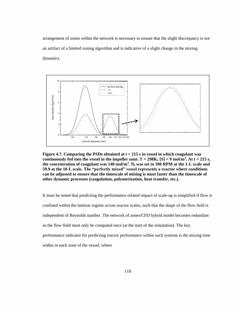
118
arrangement of zones within the network is necessary to ensure that the slight discrepancy is not
an artifact of a limited zoning algorithm and is indicative of a slight change in the mixing
dynamics.
Figure 4.7. Comparing the PSDs obtained at t = 215 s in vessel in which coagulant was
continuously fed into the vessel in the impeller zone. T = 298K; [S] = 9 mol/m3. At t = 215 s,
the concentration of coagulant was 140 mol/m3. NI was set to 100 RPM at the 1-L scale and
59.9 at the 10-L scale. The “perfectly mixed” vessel represents a reactor where conditions
can be adjusted to ensure that the timescale of mixing is must faster than the timescale of
other dynamic processes (coagulation, polymerization, heat transfer, etc.).
It must be noted that predicting the performance-related impact of scale-up is simplified if flow is
confined within the laminar regime across reactor scales, such that the shape of the flow field is
independent of Reynolds number. The network of zones/CFD hybrid model becomes redundant
as the flow field must only be computed once (at the start of the simulation). The key
performance indicator for predicting reactor performance within such systems is the mixing time
within in each zone of the vessel, where
119
,
,
,
zm z
z y
z y i
V
Q
(4.39)
Preliminary simulation work indicates that ,m i increases with reactor scale, as the rate of flow
exchanged is proportional to the surface area of the interfaces between zones; with the current
zoning algorithm, the interface surface area corresponds to the cross sectional area of the vessel.
We intend to investigate this in more detail in future work.
The original intent was to run a set of simulations at three vessel scales; however convergence of
the CFD flow field was poor at the 100 L scale when the flow field required updating. The
coagulation of particles leads to a formation of a secondary population of larger particles.
Considering a constant solids volume fraction, once the proportion of larger particles reaches a
fraction of roughly 20%, the overall viscosity of the latex will begin to drop. When the initial
PSD is specified near the loading limit, a broadening of the PSD can push the loading limit high
enough to drop the latex viscosity by a factor of 102. At the 100 L scale, this pushes operating
further into the transition regime (the tank Re approaches 1000 – 10,000) and the CFD software
was no longer capable of providing a converged solution. Limiting the study to reactor volumes
less than 100 L is not an option as the intention is to develop a framework for scale-up that can
predict performance at full commercial scale where tank volumes can reach 100 m3. Expanding
the applicability of the framework to functions in all flow regimes will also expand its
applicability to a larger range of latex concentrations. Thus the integration of a turbulent CFD
code is a necessity to harness the full capabilities of the framework once the population balance is
expanded from a coagulation model to a full emulsion polymerization kinetic model. Thus
120
efforts are underway to adapt the framework to function with CFD software that successfully
predicts fluid flow in the turbulent regime, as was attempted previously by Elgebrandt et al.17
4.6 Conclusions
The hybrid network of zones population balance/CFD computational framework demonstrated in
this work has the potential to capture information that is often difficult to isolate experimentally.
The packing model developed by Pishvaei et al.65
has been extended to provide a means of
estimating the rheological parameters of broader, more realistic PSDs. The utility of the
framework is demonstrated by using the zone-by-zone PSD information to explain some of the
trends seen in the time-evolution of the volume-averaged PSDs and the PSD of the final product.
Further improvements to the zoning algorithm are needed to ensure that model predictions are not
numerical artifacts of a simple zoning algorithm and this work is ongoing. The current framework
is limited in scope to investigating particle coagulation in vessels operating in the laminar regime
of mixing. Given the presence of turbulence in commercial vessels, expanding the framework via
the integration of a turbulent CFD code is a priority; as is the incorporation of a complete
emulsion polymerization model. Further development and refinement of the computational
framework outlined herein will yield a tool that has the potential to reduce commercialization
costs by reducing the amount of pilot plant experimentation required to ensure scalability of
product quality.
121
Chapter 5
Using a Computational Framework to Model the Scale Up of Polymer
Latex Reactors
5.1 Introduction
Polymer latex products, which are colloidally-stable dispersions of nanoscale polymer particles
dispersed in a continuous medium, are used in a wide range of applications, including paints,
adhesives and protective coatings. Due to the rising cost of petroleum-based solvents, the demand
for aqueous polymer latex products will continue to grow so long as researchers continue to
develop novel products with improved properties. Latex properties are determined by both the
formulation (e.g. choice of monomer, stabilizer, initiator, etc…) and the production process.
While all polymer latexes are created through the creation, stabilization and growth and
coagulation of particles, the precise manner in which these different phases of the process are
carried out can drastically affect the properties and value of the final product. By carefully-
controlling the nucleation and growth of particles in the reactor, particle size can be manipulated
to obtain different particle size distributions (PSDs).
From the perspective of process productivity, there is a strong interest in increasing the solids
content of existing polymer latex formulations to increase reactor throughput, reduce shipping
costs and improve the quality of end-use products.30
Most industrial latex formulations are
characterized by monodispersed PSDs and contain between 40 and 60 vol.-% solids. However,
122
by carefully controlling particle nucleation, growth and coagulation, it is possible to produce
bimodal PSDs and obtain stable products with solids content as high as 75 vol.-%. Such a high
solid content is obtainable because the small particles are engineered to fit in the interstices of the
large particle matrix.
The shape of the PSD must be properly chosen in order to obtain concentrated latexes that are
both stable and fluid (i.e. low viscosity). Due to the fine control required, the production of
bimodal latexes is challenging even at the laboratory scale.9 As reactor size is increased,
production becomes ever more challenging as it becomes increasingly difficult to maintain fine
control over the composition of the entire reactor. In many cases, the process is further
complicated by the fact that HSC latexes are non-Newtonian fluids, which makes mixing more
difficult. While there are a number of heuristic techniques available to guide production scale-
up,10, 127
these heuristics were developed for Newtonian fluids under the assumption that the flow
characteristics remain either fully-laminar or fully-turbulent during scale-up. Computational fluid
dynamic (CFD) simulation software has been widely-adapted by industry because it provides
information on the flow characteristics inside a reactor, information that often difficult to obtain
from experiment alone.13
When the flow information provided by CFD simulation is combined
with a descriptive process model, for example an emulsion polymerization process model, it
becomes possible to model the scale-up process.
Population balance models (PBMs) are considered the state-of-the-art approach for modeling the
production of polymer latexes128
because they, by their inherent structure, provide detailed
information on the PSD. While it is possible to incorporate simple reaction kinetics directly in
123
the CFD simulation by defining additional conservation equations, directly integrating a detailed
emulsion polymerization PBM into the CFD simulation is impractical as modern computers are
unable to process the resulting system of equations. An alternative approach to the direct
incorporation of the process model within the CFD simulation code is to program the models
separately, but employ them sequentially.78
The flow field computed from CFD can be used to
divide the reactor domain into a number of interacting zones,80
with each zone assumed to be
well-mixed (homogenenous). Each of these individual zones is made up of many CFD mesh cells
and the resulting network of zones (or zone grid) is much coarser than the CFD mesh. Multiple
instances of the PBM (one per zone) are then solved simultaneously on the zone grid. The rate of
material and energy transport between these zones is determined from the flow field, which may
be updated if the bulk fluid properties change appreciably (for example, due to an
increase/decrease in fluid viscosity). The hybrid multizonal CFD model framework retains the
information provided by the CFD simulation, but reduces the computational cost significantly.
The general methodology for such a framework was formalized in a series of papers published by
Bezzo et al. 78, 80, 81, 120
and its applicability was demonstrated across a small selection of chemical
and biochemical processes.
Over the past ten years, researchers have explored the potential of hybrid multizonal/CFD
frameworks to model emulsion polymerization and polymer latex coagulation. A simple, two
compartment model framework developed by Alexopoulos et al. for liquid-liquid dispersion in
suspension polymerization 83
and later emulsion polymerization 15
was one of the earliest
attempts. Later, Elgebrandt et al. 17
were the first group to adapt the general hybrid
multizonal/CFD framework to emulsion polymerization; their model was limited in scope to
124
lower solid content latexes and a simplified process model. In Chapter 4, we developed a hybrid
multizonal/CFD framework to explore the impact of non-homogeneous mixing on the controlled
coagulation of high solid content latexes. The initial work focused on the scale-up of a process
where a high solid content latex was deliberately coagulated by feeding in an electrolyte. The
study was intended to test the performance of the hybrid model framework in modeling a
controlled coagulation process, noting that the formation of undesired coagulum and scrap is an
important consideration at the industrial scale. The initial work was restricted to studying particle
coagulation (no polymerization) and reactor conditions were specified to ensure that flow
remained laminar upon vessel scale-up.
This chapter builds on the preliminary computational framework we designed to study
coagulation and examines the scale-up of a semi-batch styrene emulsion polymerization process
used to produce a latex with a bimodal particle size distribution. The focus is on the critical step
in which the small particle population is created ab initio. The framework is employed to
investigate the impact of changing the characteristic blend time on this critical nucleation stage
and the resulting final product PSD. The rate of secondary particle population is very sensitive to
the surfactant concentration, while particle stability is very sensitive to the local ion
concentration, so this particular portion of the production process is ideal for examining the
framework‟s expanded capabilities.
125
5.2 Simulation Conditions
5.2.1 Description of Process
The hybrid modeling framework, previously used assess the feasibility of scaling up a controlled
coagulation process,88
was extended to investigate a full emulsion polymerization process. While
the emulsion homopolymerization of styrene is not a particularly-intriguing process from an
industrial perspective, the kinetics of styrene polymerization are reasonably straightforward,
making it an ideal system around which to develop and test a computational framework. Most
importantly, a number of research groups have developed and experimentally-validated
population balance models for this system.99, 129
While the simulation predictions presented in this
work have not been validated experimentally, the models comprising the framework have been
validated separately in the past. The population balance process model utilizes a styrene kinetic
model that has been experimentally validated under batch99
and semi-batch103
operation. The
numerical methods used to solve the PBM were adapted from the code developed by Vale et al.8,
128 which was validated experimentally when it was used to model the homopolymerization of
vinyl chloride.7 The CFD simulation was performed with Fluent, a commercial code that has been
tested and experimentally validated to provide good predictive capabilities in a variety of mixing
applications.106, 130
The viscosity of an aqueous polymer latex is highly-dependent on the size distribution and the
concentration of particles comprising the dispersed phase. For a given concentration of particles,
the viscosity of a latex characterized by a bimodal PSD will, in general, be lower than a similar
latex with a monodispersed particle size distribution. Multimodal PSDs are generally produced
126
through the use of multiple particle nucleation steps or a single particle nucleation step in the
presence of seed particles. The first set of particles created will, ceteris paribas, grow larger than
particles that are nucleated in subsequent steps and hence the large mode of the PSD will
henceforth be referred to as the primary particle mode/population. The primary particles may be
produced in situ (one-pot) or in a separate reactor to be used as a seed (multi-pot). The creation of
secondary and tertiary particle populations is generally carried out in situ and this process step is
the most challenging and important step in the process. The surfactant and monomer are fed into
the reactor to encourage the nucleation of a secondary particle population may interact with the
primary particle population, thereby affecting the number of small particles created or even
destabilizing the primary particle lattice. For this reason the computational framework is used to
investigate the scale-up challenges associated with the nucleation of a secondary particle
population in a seeded system and the subsequent growth of both particle populations to obtain a
final product with a moderately-high dispersed-phase concentration (~ 50-wt.-% solids).
127
5.2.2 Description of the Recipes
At the start of the simulation ( 0t ), the latex is composed as follows, noting that all ingredients
are specified on a kg per kg of water (aqueous phase) basis: 0.1 kg polystyrene particles; 0.1 kg
monomer (styrene), partially swelling the particles; 3.0 × 10⁻³
kg initiator (potassium persulphate
/ KPS); 5.0 × 10⁻³
kg of anionic surfactant (sodium dodecyl sulphate / SDS). The shape of the
initial particle population is monodisperse; it follows a Gaussian distribution, with a mean
unswollen diameter of 150 nm and a standard deviation of 5 nm.
In the previous chapter we used the hybrid model framework to model coagulation with a fixed
liquid level. In this chapter, the framework is used to investigate and model one of the most
challenging steps in the production of bimodal latexes: the in situ creation of a second particle
population. To ensure the kinetic model was good, we chose to test the framework by modeling
styrene emulsion polymerization, a previously-validated system. The creation of the small
particle population involves the rapid introduction of surfactant and initiator into the reactor in
order to encourage the formation of particles via micellar nucleation. Conversely, the growth of
the bimodal population involves a much slower feed of styrene monomer into the vessel. The
particle growth process is much slower than the particle creation step. One of the limitations in
the current framework is the inability to model the rising liquid level within the reactor. This
limitation arises from the fixed nature of the zone grid; modeling a change in liquid level would
necessitate that the volume and shape of the irregularly-shaped zones be updated frequently using
a custom CFD simulation code with a moving mesh. For reactions where the relative liquid level
does not change drastically, it may be pragmatic to model the hydrodynamics using an average
liquid level. Strictly speaking, the reactor should be re-zoned frequently to account for a rising
128
liquid level. However, if the process-critical stage is relatively short, it is not unreasonable to
approximate the liquid level as constant during this stage.
Two sets of reaction simulations were run. The main set of simulations assesses the impact of a
localized reactant feed on small particle nucleation stage (evaluated by examining the PSD of the
final product) across a series of geometrically-similar reactors of varying volumetric scale. An
ancillary set of simulations was run in which the mixing limitations in the small particle
nucleation step are eliminated in order to assess the impact of scale-up (i.e. changes in the
mixing/blend time scale) on the particle growth stage. The main difference between the two
simulation scenarios is illustrated in Figure 5.1. Both sets of simulations were run at a
polymerization temperature of 70 ℃. For the purposes of simplification, it was assumed that
the process was isothermal. The assumption of isothermal operation is realistic at the
laboratory scale, but it becomes increasingly-tenuous as the amount of surface area per unit
volume of fluid will decrease as the reactor is scaled-up. Note that reactant feeds are
specified in terms of total mass added per kg of water present at the start of the reaction (kg
/ kg H2O).
In the main set of simulations, the particle nucleation phase involves feeding in 3.0×10⁻³
kg / kg
H2O of KPS and 3.0×10⁻²
SDS over a period of 4 minutes. The reactants are fed in to a localized
region near the impeller, as is illustrated in Figure 5.1. A non-instantaneous feed was chosen as it
was found that an instantaneous feed resulted in latex destabilization even at the smallest reactor
scale. Once the initiator and surfactant have been fed in, 1.1 kg / kg H2O of styrene monomer is
slowly fed into the reactor over a period 102 minutes, in order to maintain a high instantaneous
129
conversion. The total reaction time simulated is 105 minutes. At the industrial scale, reaction
times of three to four hours are common (due to heat transfer limitations), but a reaction time of
1.75 hours is reasonable for the purposes of testing the framework. The small particle nucleation
period is longer than the initiator / surfactant feed period of 4 minutes, but, it is still only a small
fraction of the overall reaction time.
In the ancillary set of simulations, at t = 0, 3.0 × 10⁻³
kg / kg H2O KPS and
3.0 × 10⁻² kg / kg H2O SDS are dispersed instantaneously through the entire vessel, along with
0.5 kg / kg H2O of styrene. After 30 minutes, 0.7 kg / kg H2O of styrene is slowly fed into the
vessel over a period of 75 minutes. The instantaneous dispersal of SDS, KPS and styrene at the
start of the simulation ensures that there are no mixing limitations during the small particle
nucleation step. Under these conditions, the framework can be used to examine the impact of
scale-up on the particle growth stage.
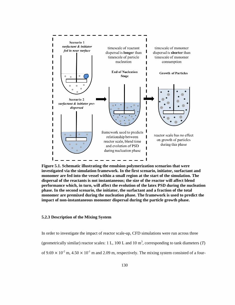
130
Figure 5.1. Schematic illustrating the emulsion polymerization scenarios that were
investigated via the simulation framework. In the first scenario, initiator, surfactant and
monomer are fed into the vessel within a small region at the start of the simulation. The
dispersal of the reactants is not instantaneous; the size of the reactor will affect blend
performance which, in turn, will affect the evolution of the latex PSD during the nucleation
phase. In the second scenario, the initiator, the surfactant and a fraction of the total
monomer are premixed during the nucleation phase. The framework is used to predict the
impact of non-instantaneous monomer dispersal during the particle growth phase.
5.2.3 Description of the Mixing System
In order to investigate the impact of reactor scale-up, CFD simulations were run across three
(geometrically similar) reactor scales: 1 L, 100 L and 10 m3, corresponding to tank diameters (T)
of 9.69 × 10⁻²
m, 4.50 × 10⁻¹
m and 2.09 m, respectively. The mixing system consisted of a four-
131
bladed 45° pitched-blade turbine and two round baffles. The liquid level was equal to 75% of the
tank diameter in the Scenario 1 simulations (e.g. ~ 7.27 × 10⁻²
m for the 1 L tank) and 85% in the
Scenario 2 simulations (e.g. ~ 8.24 × 10⁻²
m), rather than 140% as it was in Chapters 3 and 4. The
CFD simulations are run using a lower liquid level because it is assumed that the critical mixing
step occurs at an intermediate point in the process when the liquid level is lower.37
Besides the
change in the liquid level, the remaining tank proportions were the same as those listed in
Chapter 3. In the base case, a 1 L laboratory reactor, the impeller rotational speed (NI) is set to
100 RPM, which is sufficient for blending and emulsification at the laboratory scale.127
Reactor
scale-up is performed by maintaining geometric similarity, such that the relative dimensions of
the vessel and impeller system (e.g. the impeller-to-tank diameter ratio) do not change with scale-
up. Three different scale-up approaches are investigated via simulation: constant holding power
per unit volume (P/V), constant applied torque per unit volume (TQ/V) and constant reactant
blend time (blendt ). The required adjustments to the impeller rotational rate (NI) are computed
using classic heuristics,10
which assume that the fluid is Newtonian and that the reactor is
operating under fully-turbulent conditions. This set of assumptions is reasonable given that when
the secondary particle population is created, the latex solids content is below 10 vol.-% and the
tank Reynolds number at the 1-L scale is ~2.1×10⁴. This indicates that the system is likely to be
operating in (or near) the fully-turbulent regime at all reactor scales simulated. In turbulent
conditions, where viscous forces can be neglected, drag-velocity analysis can be used to show
that the volumetric power consumption of the impeller can be represented by:
3 2
I I
R
PN D
V (5.1)
It follows that the torque of the impeller, on a per-unit-volume basis can be represented by:
132
2 2Q
I I
R
TN D
V (5.2)
Maintaining a constant P/V input involves multiplying NI by a factor of 10-2/9
for every increase
in reactor volume by a factor of 10 (e.g. an increase in D by a factor of 101/3
). From Equation
(5.2) it follows that multiplying NI by a factor of 10-1/3
for every increase in reactor volume by a
factor of 10 will maintain a constant TQ/V. Under fully turbulent conditions the dimensionless
mixing time I blendN t is constant, such that NI is maintained at 100 RPM when the reactor is
scaled-up. The adjustments made to impeller rotational speed as a function of reactor scale and
scale-up objective are summarized in Table 5.1. Note that the blendt simulations were not scaled
up to 10 m3, as the motor specifications needed to operate the impeller in a 10 m
3 reactor at 100
RPM would be impossible to meet.
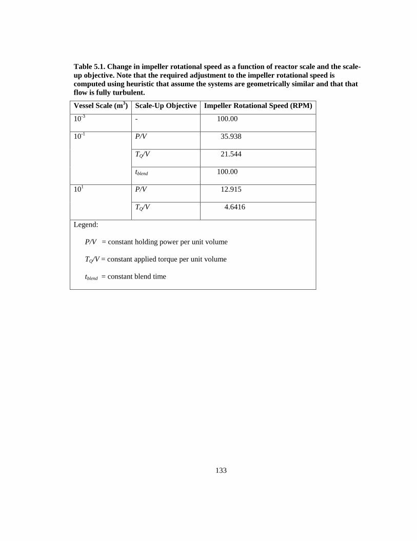
133
Table 5.1. Change in impeller rotational speed as a function of reactor scale and the scale-
up objective. Note that the required adjustment to the impeller rotational speed is
computed using heuristic that assume the systems are geometrically similar and that that
flow is fully turbulent.
Vessel Scale (m3) Scale-Up Objective Impeller Rotational Speed (RPM)
10-3
- 100.00
10-1
P/V 35.938
TQ/V 21.544
tblend 100.00
101 P/V 12.915
TQ/V 4.6416
Legend:
P/V = constant holding power per unit volume
TQ/V = constant applied torque per unit volume
tblend = constant blend time
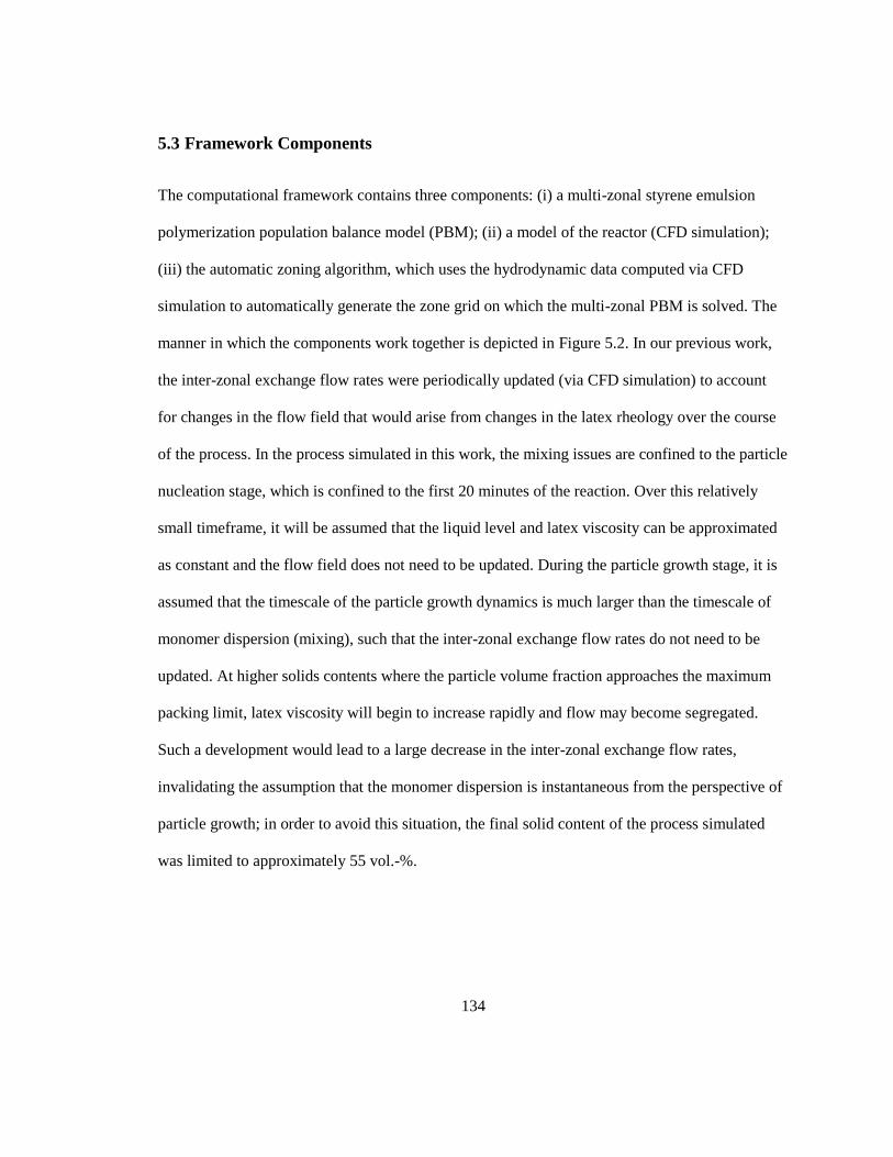
134
5.3 Framework Components
The computational framework contains three components: (i) a multi-zonal styrene emulsion
polymerization population balance model (PBM); (ii) a model of the reactor (CFD simulation);
(iii) the automatic zoning algorithm, which uses the hydrodynamic data computed via CFD
simulation to automatically generate the zone grid on which the multi-zonal PBM is solved. The
manner in which the components work together is depicted in Figure 5.2. In our previous work,
the inter-zonal exchange flow rates were periodically updated (via CFD simulation) to account
for changes in the flow field that would arise from changes in the latex rheology over the course
of the process. In the process simulated in this work, the mixing issues are confined to the particle
nucleation stage, which is confined to the first 20 minutes of the reaction. Over this relatively
small timeframe, it will be assumed that the liquid level and latex viscosity can be approximated
as constant and the flow field does not need to be updated. During the particle growth stage, it is
assumed that the timescale of the particle growth dynamics is much larger than the timescale of
monomer dispersion (mixing), such that the inter-zonal exchange flow rates do not need to be
updated. At higher solids contents where the particle volume fraction approaches the maximum
packing limit, latex viscosity will begin to increase rapidly and flow may become segregated.
Such a development would lead to a large decrease in the inter-zonal exchange flow rates,
invalidating the assumption that the monomer dispersion is instantaneous from the perspective of
particle growth; in order to avoid this situation, the final solid content of the process simulated
was limited to approximately 55 vol.-%.
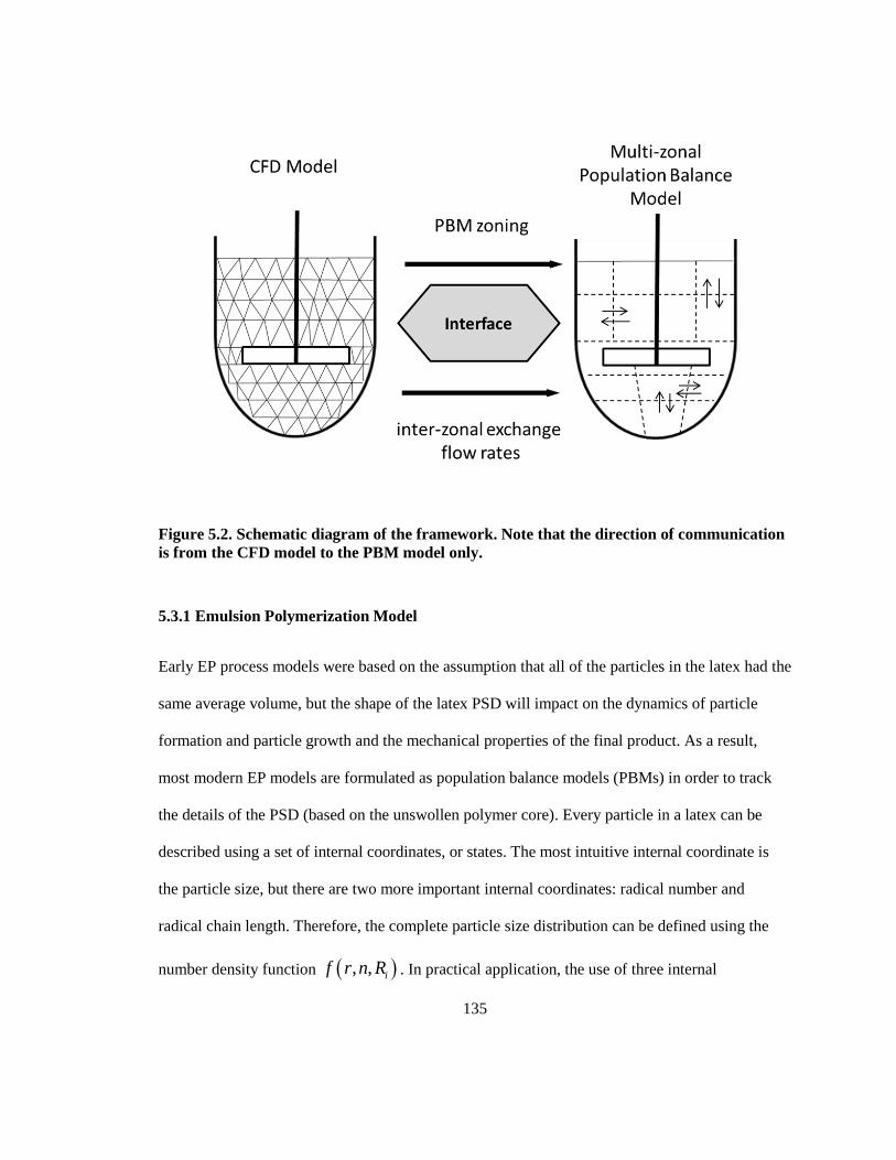
135
Figure 5.2. Schematic diagram of the framework. Note that the direction of communication
is from the CFD model to the PBM model only.
5.3.1 Emulsion Polymerization Model
Early EP process models were based on the assumption that all of the particles in the latex had the
same average volume, but the shape of the latex PSD will impact on the dynamics of particle
formation and particle growth and the mechanical properties of the final product. As a result,
most modern EP models are formulated as population balance models (PBMs) in order to track
the details of the PSD (based on the unswollen polymer core). Every particle in a latex can be
described using a set of internal coordinates, or states. The most intuitive internal coordinate is
the particle size, but there are two more important internal coordinates: radical number and
radical chain length. Therefore, the complete particle size distribution can be defined using the
number density function , , if r n R . In practical application, the use of three internal
136
coordinates yields an intractable set of multidimensional population balance equations (PBEs).7
There are two kinetic limits commonly employed to reduce the dimensionality of the PBEs to
particle size alone: the zero-one (0-1) limit and the pseudo-bulk (PB) limit.
Most commonly, encountered EP systems can be modeled using either the zero one limit or the
pseudo bulk limit.21
Refer to Section 2.2.1 in Chapter 2 for a detailed overview of these two
kinetic limits. In a „zero-one‟ system, which applies to sufficiently small particles, the entry of a
radical into a particle that already contains a growing radical is treated as an „instantaneous‟
termination. In a „pseudo-bulk system‟, which applies to both large particles and small particles in
systems with monomers that propagate very rapidly, the kinetics are treated similarly to a bulk
polymerization system. In the emulsion polymerization of styrene, experimental evidence
suggests that particles smaller than ~100 nm in diameter should be modeled with zero-one
kinetics while particles larger than 120 nm should be modeled with pseudo-bulk kinetics.85
Given
the nature of the EP processes being considered in this work, bimodal PSDs comprised of very
large and very small particles, the process model employed in this work is a hybrid zero-one /
pseudo bulk PBM.
The overall latex PSD is quantified by defining a radius number density function ( , )f r t , such
that ( , )f r t dr is the number of particles per unit volume of aqueous phase with an unswollen
radius in the range ,r r dr . As stated previously, the multi-zonal process model is designed to
model the evolution of the PSD within each individual, well-mixed zone. Therefore, the overall
137
distribution function for the reactor, ,f r t , is computed from the zone number distribution
functions ,zf r t using the volumetric average
( , )
,z z
z
z
z
V f r t
f r tV
(5.3)
Each zone within the reactor may exchange material (and energy, when applicable) with
neighbouring zones. The rate at which flow is exchanged between a zone and its neighbours is
computed from the hydrodynamic data provided via CFD simulation. To avoid unnecessary
confusion, the zone subscript for most species, kinetic parameters and kinetic coefficients will
henceforth be omitted. Unless otherwise noted, all reactant species and species-dependent
parameters and coefficients are computed separately for each zone.
To improve clarity, the process model is broken down component-by-component: (i) aqueous
phase kinetics; (ii) surfactant adsorption; (iii) monomer partitioning; (iv) particle nucleation; (v)
population balance formulation (vi) particle coagulation and (vii) latex rheology.
5.3.1.1 Aqueous Phase Kinetics
Although the locus of polymerization is the polymer particles, what occurs in the aqueous phase
plays an important part in the overall kinetic process, essentially controlling the rate of particle
formation. The key kinetic events taking place in the aqueous phase in the emulsion
polymerization of styrene that has been initiated by a persulphate initiator are schematically
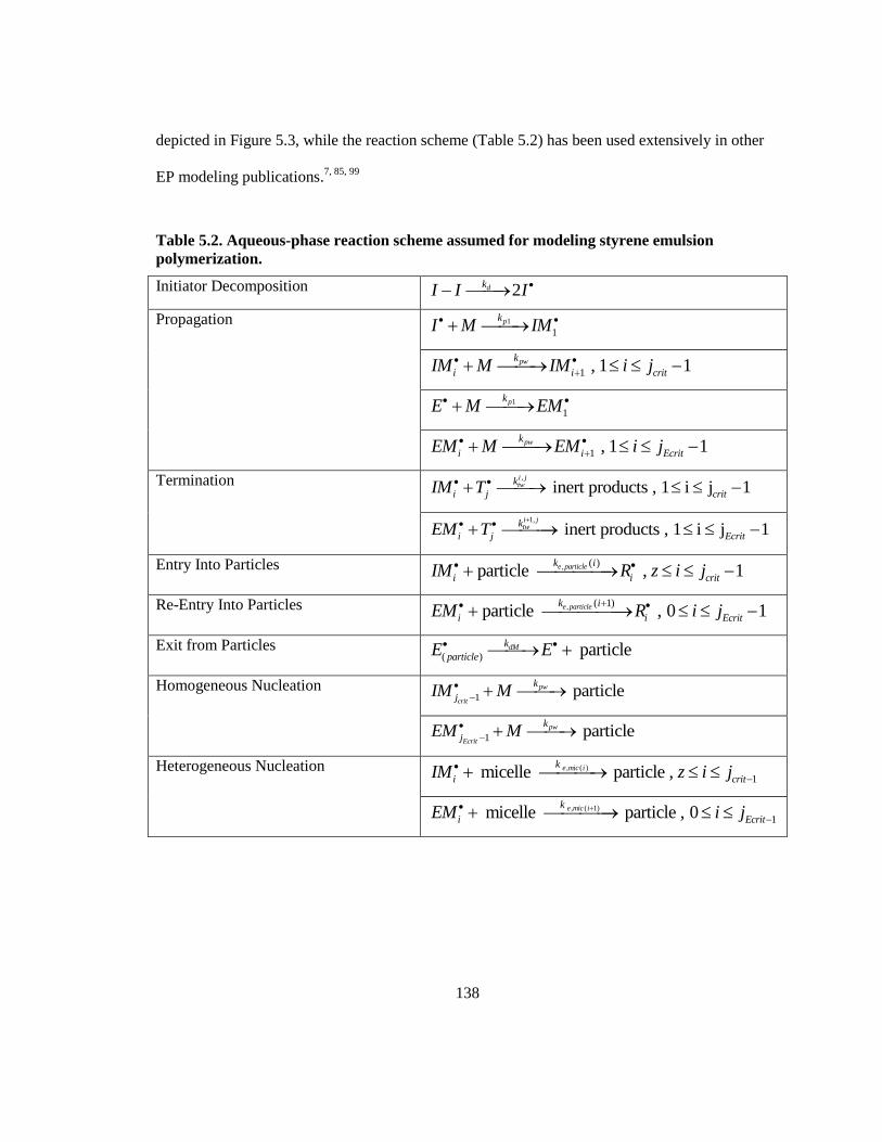
138
depicted in Figure 5.3, while the reaction scheme (Table 5.2) has been used extensively in other
EP modeling publications.7, 85, 99
Table 5.2. Aqueous-phase reaction scheme assumed for modeling styrene emulsion
polymerization.
Initiator Decomposition 2dkI I I
Propagation 1
1
pkI M IM
1 , 1 1pwk
i i critIM M IM i j
1
1
pkE M EM
1 , 1 1pwk
i i EcritEM M EM i j
Termination ,
inert products , 1 i j 1i jtwk
i j critIM T
1,
inert products , 1 i j 1i jtwk
i j EcritEM T
Entry Into Particles , ( )particle , 1e particlek i
i i critIM R z i j
Re-Entry Into Particles , ( 1)particle , 0 1e particlek i
i i EcritEM R i j
Exit from Particles ( ) particledMk
particleE E
Homogeneous Nucleation 1 particlepw
crit
k
jIM M
1 particlepw
Ecrit
k
jEM M
Heterogeneous Nucleation , ( )
1 micelle particle , e mic ik
i critIM z i j
, ( 1)
1 micelle particle , 0e mic ik
i EcritEM i j
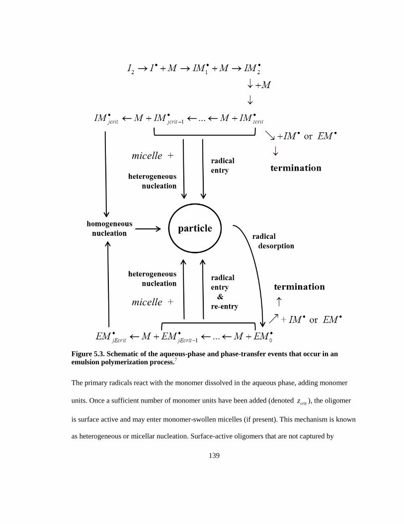
139
Figure 5.3. Schematic of the aqueous-phase and phase-transfer events that occur in an
emulsion polymerization process.7
The primary radicals react with the monomer dissolved in the aqueous phase, adding monomer
units. Once a sufficient number of monomer units have been added (denoted critz ), the oligomer
is surface active and may enter monomer-swollen micelles (if present). This mechanism is known
as heterogeneous or micellar nucleation. Surface-active oligomers that are not captured by
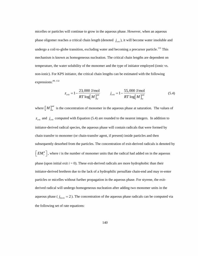
140
micelles or particles will continue to grow in the aqueous phase. However, when an aqueous
phase oligomer reaches a critical chain length (denoted critj ), it will become water insoluble and
undergo a coil-to-globe transition, excluding water and becoming a precursor particle.131
This
mechanism is known as homogeneous nucleation. The critical chain lengths are dependent on
temperature, the water solubility of the monomer and the type of initiator employed (ionic vs.
non-ionic). For KPS initiator, the critical chain lengths can be estimated with the following
expressions:99, 132
23,000 J/mol 55,000 J/mol1 1
log logcrit critsat sat
w w
z jRT M RT M
(5.4)
where sat
wM is the concentration of monomer in the aqueous phase at saturation. The values of
critz and critj computed with Equation (5.4) are rounded to the nearest integers. In addition to
initiator-derived radical species, the aqueous phase will contain radicals that were formed by
chain transfer to monomer (or chain-transfer agent, if present) inside particles and then
subsequently desorbed from the particles. The concentration of exit-derived radicals is denoted by
iEM , where i is the number of monomer units that the radical had added on in the aqueous
phase (upon initial exit i = 0). These exit-derived radicals are more hydrophobic than their
initiator-derived brethren due to the lack of a hydrophilic persulfate chain-end and may re-enter
particles or micelles without further propagation in the aqueous phase. For styrene, the exit-
derived radical will undergo homogeneous nucleation after adding two monomer units in the
aqueous phase ( 2Ecritj ). The concentration of the aqueous phase radicals can be computed via
the following set of rate equations:
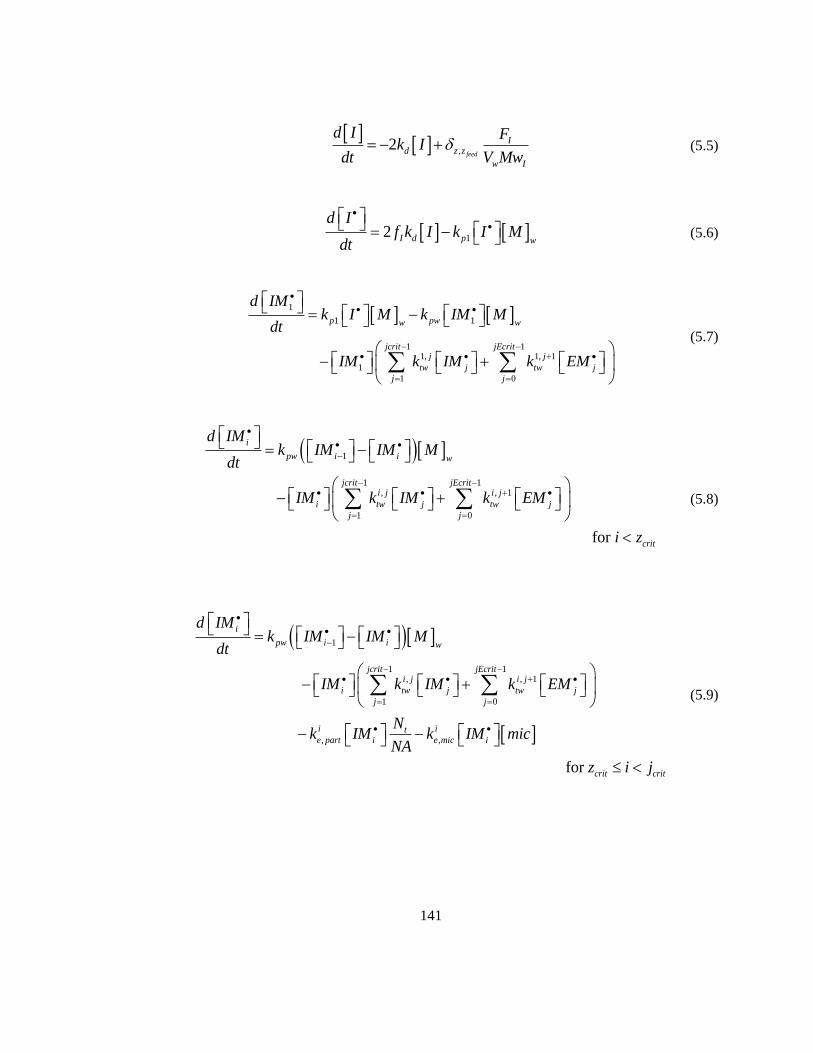
141
,2feed
Id z z
w I
d I Fk I
dt V Mw (5.5)
12 I d p w
d If k I k I M
dt
(5.6)
1
1 1
1 11, 1, 1
1
1 0
p pww w
jcrit jEcritj j
tw j tw j
j j
d IMk I M k IM M
dt
IM k IM k EM
(5.7)
1
1 1, , 1
1 0
i
pw i i w
jcrit jEcriti j i j
i tw j tw j
j j
d IMk IM IM M
dt
IM k IM k EM
for criti z
(5.8)
1
1 1, , 1
1 0
, ,
i
pw i i w
jcrit jEcriti j i j
i tw j tw j
j j
i ite part i e mic i
d IMk IM IM M
dt
IM k IM k EM
Nk IM k IM mic
NA
for crit critz i j
(5.9)
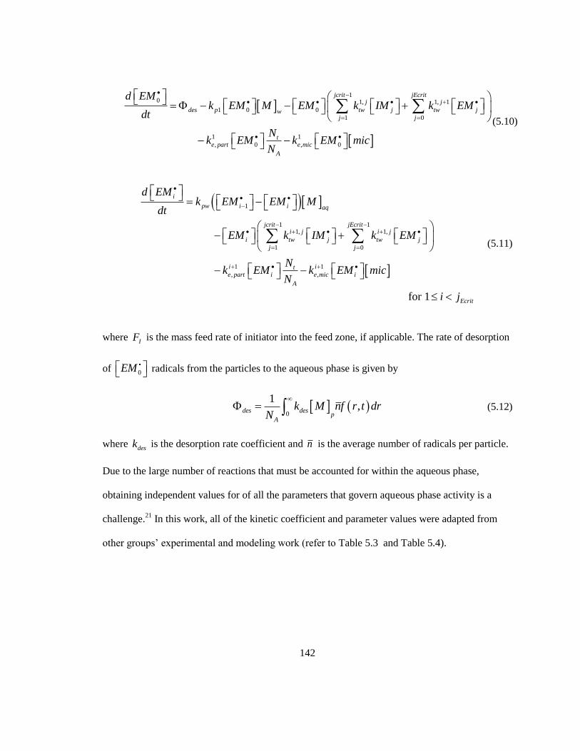
142
10 1, 1, 1
1 0 0
1 0
1 1
, 0 , 0
jcrit jEcritj j
des p tw j tw jwj j
te part e mic
A
d EMk EM M EM k IM k EM
dt
Nk EM k EM mic
N
(5.10)
1
1 11, 1,
1 0
1 1
, ,
i
pw i i aq
jcrit jEcriti j i j
i tw j tw j
j j
i ite part i e mic i
A
d EMk EM EM M
dt
EM k IM k EM
Nk EM k EM m
N
for 1 Ecrit
ic
i j
(5.11)
where IF is the mass feed rate of initiator into the feed zone, if applicable. The rate of desorption
of 0EM radicals from the particles to the aqueous phase is given by
0
1,des des
pA
k M nf r t drN
(5.12)
where desk is the desorption rate coefficient and n is the average number of radicals per particle.
Due to the large number of reactions that must be accounted for within the aqueous phase,
obtaining independent values for of all the parameters that govern aqueous phase activity is a
challenge.21
In this work, all of the kinetic coefficient and parameter values were adapted from
other groups‟ experimental and modeling work (refer to Table 5.3 and Table 5.4).
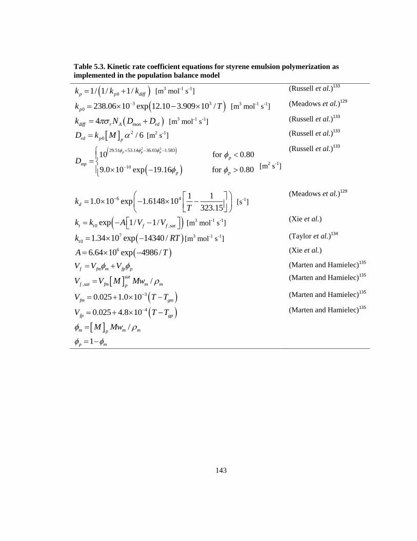
143
Table 5.3. Kinetic rate coefficient equations for styrene emulsion polymerization as
implemented in the population balance model
01/ 1/ 1/p p diffk k k [m3 mol
-1 s
-1] (Russell et al.)
133
3 3
0 238.06 10 exp 12.10 3.909 10 /pk T [m3 mol
-1 s
-1] (Meadows et al.)
129
4diff r A mon rdk N D D [m3 mol
-1 s
-1] (Russell et al.)
133
2
0 / 6rd p pD k M [m
2 s
-1] (Russell et al.)
133
2 329.51 53.14 36.03 1.583
10
10 for 0.80
9.0 10 exp 19.16 for 0.80
p p p
p
mp
p p
D
[m
2 s
-1]
(Russell et al.)133
6 4 1 11.0 10 exp 1.6148 10
323.15dk
T
[s
-1]
(Meadows et al.)129
0 ,exp 1/ 1/t t f f satk k A V V [m3 mol
-1 s
-1]
(Xie et al.)
7
0 1.34 10 exp 14340 /tk RT [m3 mol
-1 s
-1] (Taylor et al.)
134
66.64 10 exp 4986 /A T (Xie et al.)
f fm m fp pV V V (Marten and Hamielec)135
, /sat
f sat fm m mpV V M Mw
(Marten and Hamielec)135
30.025 1.0 10fm gmV T T (Marten and Hamielec)135
40.025 4.8 10fp gpV T T (Marten and Hamielec)135
/m m mpM Mw
1p m

144
Table 5.4. Miscellaneous model parameters for styrene emulsion polymerization, as
implemented in the population balance model
1.0If
107.4 10 [m] (Coen et al.)99
1 010p pk k [m3 mol
-1 s
-1]
02pw pk k [m3 mol
-1 s
-1]
105.0 10r [m] (Coen et al.)
99
31.04 10mMw [kg mol-1
]
0.30091.0 1 /636
0.7397104.152
0.2603m
T
[kg m-3
]
(Perry‟s)136
4
27
1.067 5.02 10 273.151000
1.35 10 273.15p
T
T
[kg m-3
]
(Orwol)137
0.25ijp (Gilbert)4
12
2
2
2.699 10
281.585
2.1482 10 1.28078.4 281.585
mwD T
T
T
[m2 s
-1]
(Meadows et
al.)129
184.95gmT [K] (Marten and
Hamielec)135
366.65gpT [K] (Marten and
Hamielec)135
2.1sb [m3/mol] (Coen et al.)
99
283.85 10sV [m3]
138
/m m m AV Mw N [m3]
41.68 10micK [mol-1
] 138
98.0 10 [m]Fr
(Coen et al.)
The aqueous phase termination rate coefficient is computed with the modified von
Smoluchowski4 equation:
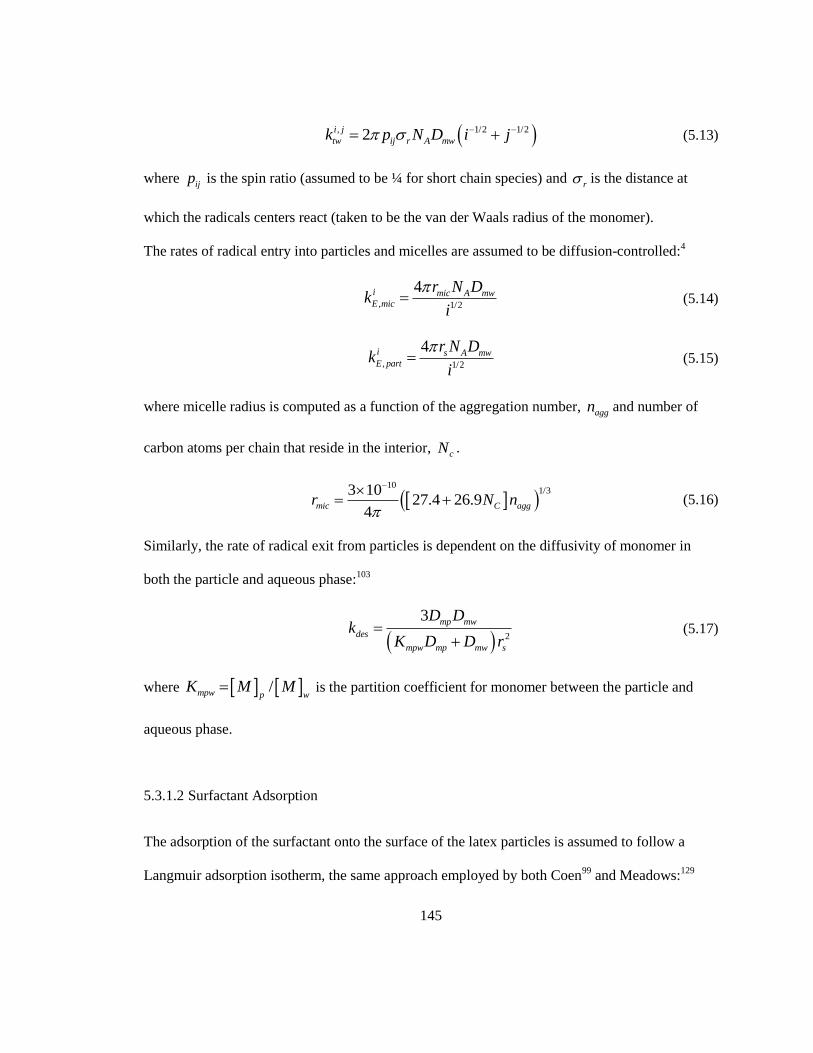
145
, 1/2 1/22i j
tw ij r A mwk p N D i j (5.13)
where ijp is the spin ratio (assumed to be ¼ for short chain species) and
r is the distance at
which the radicals centers react (taken to be the van der Waals radius of the monomer).
The rates of radical entry into particles and micelles are assumed to be diffusion-controlled:4
, 1/2
4i mic A mwE mic
r N Dk
i
(5.14)
, 1/2
4i s A mwE part
r N Dk
i
(5.15)
where micelle radius is computed as a function of the aggregation number, aggn and number of
carbon atoms per chain that reside in the interior, cN .
10
1/33 1027.4 26.9
4mic C aggr N n
(5.16)
Similarly, the rate of radical exit from particles is dependent on the diffusivity of monomer in
both the particle and aqueous phase:103
2
3 mp mw
des
mpw mp mw s
D Dk
K D D r
(5.17)
where /mpw p wK M M is the partition coefficient for monomer between the particle and
aqueous phase.
5.3.1.2 Surfactant Adsorption
The adsorption of the surfactant onto the surface of the latex particles is assumed to follow a
Langmuir adsorption isotherm, the same approach employed by both Coen99
and Meadows:129
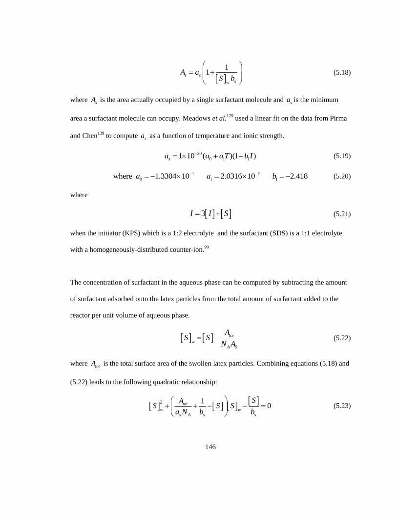
146
11s s
sw
A aS b
(5.18)
where sA is the area actually occupied by a single surfactant molecule and
sa is the minimum
area a surfactant molecule can occupy. Meadows et al.129
used a linear fit on the data from Pirma
and Chen139
to compute sa as a function of temperature and ionic strength.
20
0 1 11 10 ( )(1 )sa a a T b I (5.19)
1 1
0 1 1where 1.3304 10 2.0316 10 2.418a a b (5.20)
where
3I I S (5.21)
when the initiator (KPS) which is a 1:2 electrolyte and the surfactant (SDS) is a 1:1 electrolyte
with a homogeneously-distributed counter-ion.99
The concentration of surfactant in the aqueous phase can be computed by subtracting the amount
of surfactant adsorbed onto the latex particles from the total amount of surfactant added to the
reactor per unit volume of aqueous phase.
tot
wA S
AS S
N A (5.22)
where totA is the total surface area of the swollen latex particles. Combining equations (5.18) and
(5.22) leads to the following quadratic relationship:
2 1
0tot
w ws A s s
SAS S S
a N b b
(5.23)
147
Similarly, the positive root of equation (5.23) is used to compute w
S . The micelle
concentration can then be computed with the following relationship:
max 0, w
agg
S CMCmic
n
(5.24)
The critical micelle concentration, often expressed as a constant in EP models, will change, in the
presence of additives such as salt and as a function of temperature. In particular, the CMC is very
sensitive to added electrolyte; the addition of 1×10⁻²
mol/L of NaCl reduces the CMC of SDS by
more than a factor of 2.5.140
The fit performed by Meadows et al.129
on the extensive data
compiled by Mukerjee and Mysels140
for sodium dodecyl sulphate (SDS) is not a first principles
model, but it is acceptable for the purposes of this work.
2 0 10 1 2
0 1
b b ICMC a a T a T
c c I
(5.25)
1 4 6
0 1 2
0 1 0 1
where 1.539 10 9.7902 10 1.6391 10
0.9995 1.1955 1.0 29.34
a a a
b b c c
It has been found that in the case of sodium dodecyl sulphate (SDS) and anionic surfactants in
general, the addition of salt and other impurities will cause aggregation number, and thus micelle
size to increase. Bales et al.141
developed the following semi-phenomenological model to
compute the aggregation number as a function of surfactant and salt concentration:
1/4
0
0.27 0.73 349.5 w
agg agg
S S NaCl In n
CMC
(5.26)
where0CMC is the critical micelle concentration in the absence of added ionic species. The
relationship presented by Bales has been modified to include the contributions of the initiator,
potassium persulphate. This falls in line with the data presented in other literature, such as
148
Giannetti et al.138
, where the contributions of all cationic species are taken into account when
computing the CMC andaggn . Water insoluble species may be solubilized within the micelles,
increasing the aggregation number until the solubilisation limit is reached. For styrene monomer,
for example, the number of additional solubilized molecules per micelle, AX , is given as follows:
,A mic eq wX K M (5.27)
where ,mic aqK is the partition coefficient of styrene between the micelle and aqueous phases.
138
This relationship can be used to compute the increase in aggn by evaluating the change in micelle
area per head group before and after monomer addition138
:
2 magg A
S
Vn X
V (5.28)
where sV and
mV are the hydrophobic volumes of the surfactant tail (C12 for SDS) and the
monomer, respectively. In spite of the highly precise manner in which is possible to compute the
micelle surface area for particle capture, it is important to note that industrial surfactants will
contain a combination of anionic and non-ionic components and impurities. There will likely be
variations in the CMC and aggregation number from one batch of surfactant to another, thus, in
industrial application, parameters determined from in-house experimental measurement should
provide improved predictive capability over the use of Equations (5.25) to (5.28). If the model is
being developed to perform over a wide range of temperatures and in the presence of added
electrolytes, the empirical models are preferred to experimental constants, as the CMC and aggn
values are likely be sensitive to the conditions inside the reactor.
149
5.3.1.3 Monomer Balance
The total mass of monomer in the system is given by:
, feed
mz z m pw pp m m m
dmF R R Mw V Q
dt m (5.29)
where mF is the mass feed rate of monomer into the feed zone, z mQ m is the net rate of
monomer flowing into zone z due to flow exchanged with neighbouring zones, and mMw is the
molar mass of monomer. The total rate of monomer consumption in each zone, pR is a sum of
the rate of polymerization in the particles ppR and in the aqueous phase
pwR :
0( ) ( , )
p
pp zPA
kR M r nf r t dr
N
(5.30)
11
1 0
2crit Ecritj j
pw I d pw i iwi i
R f k I k M IM EM
(5.31)
The mass of monomer inside the swollen polymer particles is computed with the following
expression:
3
, ,0
4,
3m p m w sp sat
m Mw V M r f r t dr
(5.32)
Initially, p
M is set to equal sat
pM , which is assumed to be a function of particle radius:
4
,
( ) tanh /sat sat
fp pM r M r r
(5.33)
150
where fr is a parameter that expresses the radius at which p
M approaches the limiting value
of sat
pM . The concentration of monomer in the aqueous phase,
wM ,is also initially set to
sat
wM
to provide an initial estimate of the amount of monomer dissolved in the aqueous phase
,m w m wwm M Mw V (5.34)
The mass of monomer droplets in the system is
, , ,m d m m w m pm m m m (5.35)
If , 0m dm , monomer droplets are present in the system. If
, 0m dm , a new estimate of ,m Pm is
computed from
, ,m p m m wm m m (5.36)
p
M is subsequently computed with the following expression:
,
3
,0
4,
3
m P
p
m p m p
mM
Mw r f r t dr m
(5.37)
where the denominator of Equation (5.37) is an expression for computing the swollen volume of
the polymer particles. w
M is then updated using the semi-empirical expression developed by
Vanzo et al.:142
0.6
pw
sat sat
w p
MM
M M
(5.38)
151
Subsequently, ,m wm is updated using Equation (5.34) and a new value of
,m pm is computed from
Equation (5.36). The new estimate of ,m pm is compared to the value at the previous iteration and
the iterative procedure ends once the relative change in ,m pm is less than a specified tolerance.
5.3.1.4 Particle Nucleation
As schematically shown in Figure 5.3 and discussed above, initiator derived radicals and transfer-
derived radicals that reach a surface-active length may enter into micelles, resulting in
heterogeneous (micellar) nucleation. The rates of heterogeneous nucleation due to initiator-
derived and exit-derived radicals are given as follows:
1
, ,
jcriti
mic I E mic i
i z
R mic k IM
(5.39)
1
1
, ,
0
jEcriti
mic E E mic i
i
R mic k EM
(5.40)
When initiator-derived and exit-derived radicals reach their respective critical lengths, they will
precipitate out, forming precursor particles. The rates of homogeneous nucleation are given by:
hom, 1I pw jcrit WR k IM M
(5.41)
hom, 1E pw jEcrit WR k EM M
(5.42)
The total rate of particle nucleation is the summation of Equations (5.39) - (5.42):
, , hom, hom,nuc mic I mic E I ER R R R R (5.43)
152
All nucleated particles are assumed to have the same unswollen radius, nucr as the numerical
predictions are insensitive to the value of nucr , provided it is chosen pragmatically (e.g. 5 nm).
99
Therefore, nucr was computed with the following expression:
1
33
4
crit mnuc mic
A P
j Mwr r
N
(5.44)
5.3.1.5 Particle Population Balance Model
For a given zone z, the EP PBEs can be written in a general form by defining a vector
distribution, ( , )z r tf that groups the individual number density functions. For analytical
solutions, the PBEs are often written using particle volume as an internal coordinate, but for
numerical solutions, it is preferable to use the un-swollen particle radius as an internal coordinate.
The PBM employed is a hybrid of the zero-one and pseudo-bulk model. For each zone in the
reactor, the overall hybrid balance expression can be written as follows:
0 1
( , ) ( ) ( , ) 1 ( ) ( , )z s z s z
MP PB
r t r r t r r tt t t
f f f m (5.45)
where m is specified to ensure that the dimensionality of the pseudo-bulk contribution matches
that of the zero-one contribution:
,1,0 ,1
( , )( , ) ( , )
( , ) ( , ) ( , )
T
z pz z m
z z z
f r tf r t f r t
f r t f r t f r t
m (5.46)
In the zero-one model, the overall distribution is a sum of the individual distributions, such that
,0 ,1 ,1( , ) ( , ) ( , ) ( , )z z z P z Mf r t f r t f r t f r t (5.47)
153
where ,0 ( , )zf r t is the distribution of particles containing no free radicals,
,1 ( , )z Pf r t is the
distribution of particles containing a polymeric free radical and ,1 ( , )z Mf r t is the distribution of
particles containing a monomer derived free radical.
The transition between zero-one kinetics and pseudo-bulk kinetics is a gradual process. The
Gilbert group suggested that a cross-over radius range is 50 nm – 60 nm for styrene.85, 143
The
smoothing function, ( )sr , is formulated such that the dynamics of particles with a swollen
radius less than 50 nm are modeled exclusively using zero-one kinetics and the dynamics of all
particles with swollen radii larger than 60 nm are modeled using pseudo-bulk kinetics. Within the
cross-over range, the overall particle dynamics are smoothed using the following function:
3 3
3 3
1.0 for
( ) for
0.0 for
s l
u ss l u
u l
s u
r r
r rr r r r
r r
r r
(5.48)
where 50 nmlr and 60 nm.ur Given that the particle-specific termination rate coefficient
is a function of particle volume rather than particle radius, a smoothing function that is linear with
respect to particle volume was deemed to be acceptable for the demonstrative purposes of this
work. A smoothing function based on the error function was tested as well, but the numerical
predictions did not change noticeably.
Both the 0-1-MP and PB terms take on the same general form, that of a system of linear
hyperbolic balance laws:
154
( , ) ( , ) ( , ) ( , , ) for X = 0-1, PBz z z z z XXX
r t r r t rt t
f r y f s f y (5.49)
2( , ) ( , ) / 4r r rr y v y (5.50)
The subscript X is omitted in subsequent expressions, but it should be noted that the following
terms will be strongly influenced by the kinetic limit because they are functions of n : (i) ( , )rv y ,
(ii) ppR and (iii)
desk .
Within the zero-one framework, the average number of radicals per particle is computed from the
particle number density distributions directly:
10 1
( , )( , )
( , )
f r tn r t
f r t (5.51)
where 1 1 1( , ) ( , ) ( , )P Mf r t f r t f r t .
There are two widely-used expressions available for computing n under pseudo-bulk kinetic
conditions.21
The method employed in this work is the steady-state approximation that was
originally published by O‟Toole almost fifty years ago.144
Under the assumption that CLD
termination may be neglected and that the rates of radical entry, desorption and termination are
much faster than nucleation, coagulation, growth and inflow/outflow, ( , )n v t 144 can be computed
as:
1( , ) ( ) / 4 ( )PB m mn r t aI a I a (5.52)
where 8 /A ta N v k and /des A tm k N v k are the argument and order of the modified Bessel
function of the first kind ( )mI a 7, respectively.
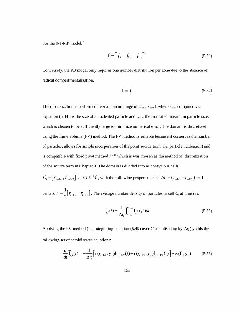
155
For the 0-1-MP model:7
0 1 1
T
p mf f f f (5.53)
Conversely, the PB model only requires one number distribution per zone due to the absence of
radical compartmentalization.
ff (5.54)
The discretization is performed over a domain range of [rnuc, rmax], where rnuc, computed via
Equation (5.44), is the size of a nucleated particle and rmax, the truncated maximum particle size,
which is chosen to be sufficiently large to minimize numerical error. The domain is discretized
using the finite volume (FV) method. The FV method is suitable because it conserves the number
of particles, allows for simple incorporation of the point source term (i.e. particle nucleation) and
is compatible with fixed pivot method,8, 128
which is was chosen as the method of discretization
of the source term in Chapter 4. The domain is divided into M contiguous cells,
1/2 1/2, , 1i i iC r r i M , with the following properties: size 1/2 1/2i i ir r r cell
centers 1/2 1/2
1
2i i ir r r . The average number density of particles in cell Ci at time t is:
1/2
1/2,
1( ) ( , )
i
i
r
z i zr
i
t r t drr
f f (5.55)
Applying the FV method (i.e. integrating equation (5.49) over Ci and dividing by ir ) yields the
following set of semidiscrete equations:
, 1/2 , 1/2 1/2 , 1/2
1( ) ( , ) ( ) ( , ) ( ) ( , )z i i z z i i z z i i z z
i
dt r t r t
dt r
f r y f r y f s f y (5.56)
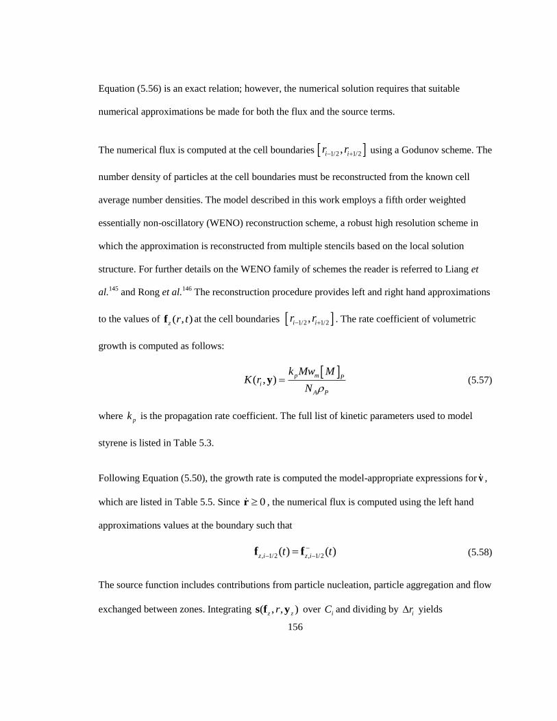
156
Equation (5.56) is an exact relation; however, the numerical solution requires that suitable
numerical approximations be made for both the flux and the source terms.
The numerical flux is computed at the cell boundaries 1/2 1/2,i ir r using a Godunov scheme. The
number density of particles at the cell boundaries must be reconstructed from the known cell
average number densities. The model described in this work employs a fifth order weighted
essentially non-oscillatory (WENO) reconstruction scheme, a robust high resolution scheme in
which the approximation is reconstructed from multiple stencils based on the local solution
structure. For further details on the WENO family of schemes the reader is referred to Liang et
al.145
and Rong et al.146
The reconstruction procedure provides left and right hand approximations
to the values of ( , )z r tf at the cell boundaries 1/2 1/2,i ir r . The rate coefficient of volumetric
growth is computed as follows:
( , )p m P
i
A P
k Mw MK r
N y (5.57)
where pk is the propagation rate coefficient. The full list of kinetic parameters used to model
styrene is listed in Table 5.3.
Following Equation (5.50), the growth rate is computed the model-appropriate expressions for v ,
which are listed in Table 5.5. Since 0r , the numerical flux is computed using the left hand
approximations values at the boundary such that
, 1/2 , 1/2( ) ( )z i z it t
f f (5.58)
The source function includes contributions from particle nucleation, particle aggregation and flow
exchanged between zones. Integrating ( , , )z zrs f y over iC and dividing by
ir yields
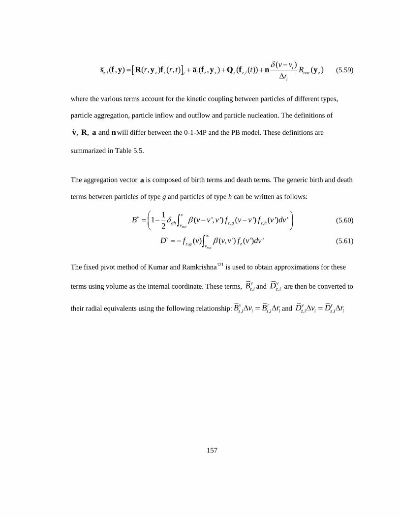
157
, ,
( )( , ) ( , ) ( , ) ( , ) ( ( )) ( )i
z i z z i z z z z i nuc zii
v vr r t t R
r
s f y R y f a f y Q f n y (5.59)
where the various terms account for the kinetic coupling between particles of different types,
particle aggregation, particle inflow and outflow and particle nucleation. The definitions of
, , and v R a nwill differ between the 0-1-MP and the PB model. These definitions are
summarized in Table 5.5.
The aggregation vector a is composed of birth terms and death terms. The generic birth and death
terms between particles of type g and particles of type h can be written as follows:
, ,
11 ( ', ') ( ') ( ') '
2 nuc
vv
gh z g z hv
B v v v f v v f v dv
(5.60)
, ( ) ( , ') ( ') 'nuc
v
z g zv
D f v v v f v dv
(5.61)
The fixed pivot method of Kumar and Ramkrishna121
is used to obtain approximations for these
terms using volume as the internal coordinate. These terms, ,
v
z iB and ,
v
z iD are then be converted to
their radial equivalents using the following relationship: , ,
v r
z i i z i iB v B r and , ,
v r
z i i z i iD v D r
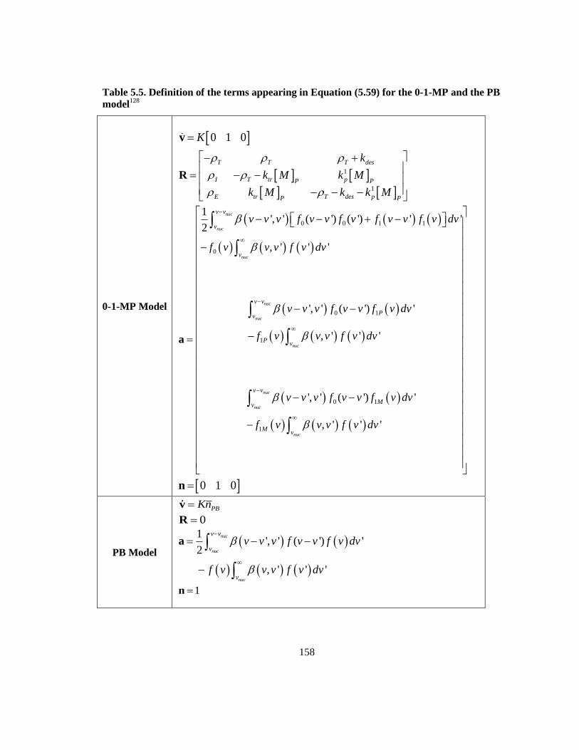
158
Table 5.5. Definition of the terms appearing in Equation (5.59) for the 0-1-MP and the PB
model128
0-1-MP Model
0 1 0Kv
1
1
T T T des
I T tr pP P
E tr T des pP P
k
k M k M
k M k k M
R
0 0 1 1
0
0 1
1
0 1
1
1', ' ( ') ( ') ' '
2
, ' ' '
', ' ( ') '
, ' ' '
', ' ( ') '
, ' ' '
nuc
nuc
nuc
nuc
nuc
nuc
nuc
nuc
nuc
v v
v
v
v v
Pv
Pv
v v
Mv
Mv
v v v f v v f v f v v f v dv
f v v v f v dv
v v v f v v f v dv
f v v v f v dv
v v v f v v f v dv
f v v v f v dv
a
0 1 0n
PB Model
PBKnv
0R
1', ' ( ') '
2
, ' ' '
nuc
nuc
nuc
v v
v
v
v v v f v v f v dv
f v v v f v dv
a
1n
159
The kinetic coupling term is approximated using the simplest solution, a second order
approximation:
2
,( , ) ( , ) ( , ) ( ) ( )z z i z z i iir r t r t O r R y f R y f (5.62)
As noted by Vale7, this formulation is convenient for integration over time. The cell pivots are the
cell centers,iv , where
34 / 3i iv r ; the particles in iC are concentrated at the representative
pivot points such that, for particles of type g:
, ,
1
( , ) ( )M
g
z g z i i
i
f v t N v v
(5.63)
,
1
( , ) ( )M
z z i i
i
f v t N v v
(5.64)
( )
( )v ii
i
N tf t
v
(5.65)
, ,( ) ( )g
z i z igN t N t (5.66)
When particles of size jv and
kv aggregate together, their combined volume, ˆj kv v v , may
fall between two pivot points. iC will receive a contribution from every particle born between the
range 1 1,i iv v . For particles born between 1iv and
iv such that 1ˆ
i iv v v , the fraction
contributed to iC is
1
1
ˆˆ( , ) i
i
i i
v va v v
v v
(5.67)
For particles born between 1iv and
iv , the fraction contributed to iC follows a similar
expression:
160
1
1
ˆˆ( , ) i
i
i i
v vb v v
v v
(5.68)
These lever-rule expressions ensure that the particle number and mass are preserved. For fixed
grids, such as the ones employed in this work, the particle combinations that result in a particle
from cells i and j being born in 1 1,i iv v and the associated ˆ( , )ia v v and ˆ( , )ib v v values are
computed only once: at the start of the simulation.
The discretized birth and death terms are obtained by integrating Equations (5.60) and (5.61) over
iC , dividing by ir and substituting in Equations (5.63) and (5.64):
1
1
1
, ,
,ˆ
, 1
, ,
,ˆ
ˆ( ) ( , , )
1, g h
ˆ( ) ( , , )
i i
i i
i jg h
j k z z j z k
j kv v vr
z i i ji g h
j k z z j z k
j kv v v
a v r r N N
Br
b v r r N N
y
y (5.69)
1
1
1
, , ,
,ˆ
, 1
, , ,
,ˆ
1ˆ(1 ) ( ) ( , , )
21
1ˆ(1 ) ( ) ( , , )
2
i i
i i
i jg g
j k j k z z j z k
j kv v vr
z i i ji g g
j k j k z z j z k
j kv v v
a v r r N N
Br
b v r r N N
y
y
(5.70)
, , ,
1
1( ) ( , , ) ( )
Mr g
z i z i i j z z j
ji
D N t r r N tr
y (5.71)
The aggregation vector is computed from the discretized birth and death terms, Equations (5.69) -
(5.71), with the specific expressions being dependent on whether the terms are being calculated
161
for the 0-1-MP component or the PB component of the PBM. Note that Equation (5.69) stands in
for the terms where different two particles of different classes of particles are aggregating (e.g.
0N with 1PN ), while Equation (5.70) stands in for the terms where particles of the same class
are aggregating with each other (e.g. 1PN with
1PN ).
The flow exchange termQ is computed using the connectivity and flow exchange information
computed with the automatic zoning algorithm.
, , ,
, ,
( )( ( )) ( ) ,
y z y i z i
z i z y
y yy zy z y z
q tQ t t q y z
V V
Z Zf f
f Z (5.72)
where ,y zq is the rate of flow in the direction from zone y into zone z. Note that material between
connected zones is exchanged in both directions, with the net rate of flow exchanged being equal
to , ,y z z yq q . If zones are unconnected, , , 0y z z yq q .
Equations (5.56) and the continuous phase mass balance equations ( )zy are integrated with time
using an implicit-explicit (IMEX) solution scheme. The kinetic coupling terms ( )Rf are very
stiff and are handled implicitly, whereas the coagulation, advection and interzonal flow terms are
highly non-linear and are therefore treated explicitly. A variable step-size, first order forward-
backward Euler scheme was adopted to compute1n
f
t n+1 n n n+1
E If f L L (5.73)
Both the pseudo-bulk and zero-one kinetic models contain explicit components that are gathered
into a vector:
162
0 1( ) 1 PB
i i i i ir r e e me (5.74)
The inclusion of m changes the dimensionality of PB
ie to match that of 0 1
i
e , such that the only
term that differs between PB
ie to 0 1
i
e is the advective term, such that the explicit vector can be
computed as follows:
0 1,1
, 1/2 1/2 1/2 1/2
1( ( ))
PBi i i
i nuc i z i i i i i
i i
r rR Q t
r r r
e n a f h h h h (5.75)
The time discretization then reads as:
1 1 1
, , , ,( , )n n n n n
i z i z i z i z i zt r f f e R y f (5.76)
The implicit component is linear in f , so Equation (5.76) may be re-arranged to yield a
relationship explicit in 1
,
n
i z
f :
1
1 1
, , ,( , )n n n n
i z i z i z i zt r t
f I R y f e (5.77)
The inverse matrices appearing in (5.77) are computed analytically. Since R is initially known at
tn and not at t
n+1, an iterative procedure is used, whereby R
n, calculated at t
n with n
y is used to
calculate an approximation of 1n
f . This approximation is used to compute an approximation of
1ny which is then used to compute another approximation of R
n+1. The cycle is repeated until a
specified convergence is achieved. Typically, the number of iterations required is small and the
computational resources required are insignificant with respect to that of evaluating ,
n
i ze .
163
5.3.1.6 Coagulation Kernel
Modeling the rate of particle coagulation in emulsion polymerization systems is a challenge due
to the complexity of the phenomena involved and the lack of suitable physical models. The
widely-used DLVO framework does not always provide good quantitative predictions when it is
used to model the aggregation rate of colloids. Regardless, it has been shown that many
experimental results cannot be predicted in a physically-coherent manner without the inclusion of
a coagulation kernel.7 In many cases it is possible to fit certain model parameters (such as the
Hamaker constant) to obtain coagulation rate coefficients that correctly predict experimental
results, even in conditions where DLVO theory may not be applicable. For further information on
the use of DLVO-theory based coagulation kernels, refer to Vale & McKenna.8
The coagulation kernel used in this study is the same coagulation kernel that was outlined in
detail in the previous chapter in Section 4.2.3. The coagulation rate coefficient between two
particles of size i and j, βij is computed from the Fuchs-modified Muller-Smoluchowski94
equation:
2
2 3
jiBij
s ij j i
rrk T
W r r
(5.78)
where s is the viscosity of the dispersion medium and
Bk is the Boltzmann constant. The
Fuchs‟ stability ratio (Wij) , which is the inverse of the collision efficiency, accounts for the
presence of colloidal interactions between the particles. The normalized stability ratio is
computed with the expression:123
164
int
20
20
( )exp
( )exp
B
ij
A
B
V s
k Tds
sWV s
k Tds
s
(5.79)
As defined in Equation (5.79), ijW is equal to unity in the complete absence of repulsive
potential, which is helpful when model predictions are compared against experimental data. To
simplify matters, the hydrodynamic interaction effects not included in this coagulation model,
although they could be incorporated in the stability model (see Section 3.2 in Chapter 3 for
details). The expressions used to compute the ionic charge distribution surrounding the latex
particles include additional terms to account for concentration effects at higher solid contents.
The modified expression for the inverse Debye length is:
2 24
1
totA
B
AN I
e e
k T
(5.80)
Based on the experimental data obtained by Kemmere et al. for high solid content styrene
emulsion polymerization systems,41
the contributions of shear-induced (orthokinetic) coagulation
were neglected in favour of a strictly Brownian (perikinetic) aggregation kernel. Orthokinetic
coagulation is thought to be prevalent in systems where very larger particles (greater than ~ 1 μm
in diameter) are exposed to regions of high shear rates (γ > 100 s-1
). Melis et al.44
numerically
solved the generalized Fuchs-Smoluchowski diffusion-convection equation for a pair of spherical
particles located in an extensional flow field and found that an adjusted particle Peclet number
could be used to determine whether orthokinetic coagulation is likely to be prevalent under a
165
given set of conditions. In a subsequent modeling effort (the EP of vinyl acetate), Melis et al. note
that the average particle Peclet number computed for a reaction at the laboratory scale is much
lower than the threshold beyond which orthokinetic coagulation must be taken into account.42
As
was concluded in Chapter 3, it would be incorrect to assume that the orthokinetic mechanism can
be neglected under most conditions. There are a number of semi-empirical combined coagulation
kernels available in the literature 43, 45, 46
and Lattuada and Morbidelli recently developed a kernel
that can be applied in both shear-dominated and Brownian-dominated conditions.47
Unfortunately
the Lattuada and Morbidelli is much more computationally-intensive due to iterative procedure
required to compute the parameters that account for hydrodynamic interactions between particles.
5.3.1.7 Latex Rheology
The non-Newtonian rheology was modeled with the Carreau-Yasuda model, which has been
shown to correctly capture the shearing behavior of concentrated latexes;5
0
1 /
( ) ( ) for
1thm a
a
t t
(5.81)
where 0 is the zero-shear viscosity,
is the infinite-shear viscosity, is the characteristic
time for the onset of shear-thinning andth is the shear rate beyond which the latex will begin to
shear thicken. The adjustable parameters a and m were set to 1.0 and 0.65, respectively, which
has been shown to provide the best fit to their experimental data.5 The four model parameters
0 , , ,1/ th are dependent on the latex solid content ( ) and the (PSD-dependent)
166
effective maximum packing fraction (m ,) according to general form of the Krieger-Dougherty
equation.
,
0
,
( )( ) 1 , , , 1/
( )
m
s th
m
tt
t
(5.82)
The intrinsic viscosity ([η]) and hard sphere maximum packing fraction parameters ( ,) needed
to utilize Equation (5.82) can be found in Table 3.1 in Chapter 3.
The maximum packing fraction of a polymer latex made up of m discrete particle sizes was
calculated using the approach proposed by Pishvaei et al.65
The formulae are not listed here as
they are the exact same as those appearing in Chapter 4; refer to Equations (4.29) to (4.34) in
Section 4.2.5. For a more detailed background on modeling the packing characteristics of latexes
with bimodal and multimodal PSDs, refer to Section 2.2.4 in Chapter 2.
5.3.2 CFD Model
The mixing time in reactors can be measured both experimentally and numerically using transient
concentration (homogenization) curves. The homogenization curves are computed via CFD
simulation in two steps. First, the fully-developed flow field is computed assuming that the latex
can be simulated as a single-phase fluid. After the fully-developed flow field has been computed,
the transient dispersion of a buoyantly-neutral tracer species is superimposed on the flow field to
determine the homogenization curves.
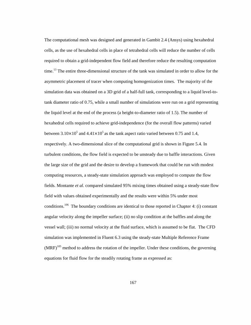
167
The computational mesh was designed and generated in Gambit 2.4 (Ansys) using hexahedral
cells, as the use of hexahedral cells in place of tetrahedral cells will reduce the number of cells
required to obtain a grid-independent flow field and therefore reduce the resulting computation
time.13
The entire three-dimensional structure of the tank was simulated in order to allow for the
asymmetric placement of tracer when computing homogenization times. The majority of the
simulation data was obtained on a 3D grid of a half-full tank, corresponding to a liquid level-to-
tank diameter ratio of 0.75, while a small number of simulations were run on a grid representing
the liquid level at the end of the process (a height-to-diameter ratio of 1.5). The number of
hexahedral cells required to achieve grid-independence (for the overall flow patterns) varied
between 3.10×10⁵ and 4.41×10
5 as the tank aspect ratio varied between 0.75 and 1.4,
respectively. A two-dimensional slice of the computational grid is shown in Figure 5.4. In
turbulent conditions, the flow field is expected to be unsteady due to baffle interactions. Given
the large size of the grid and the desire to develop a framework that could be run with modest
computing resources, a steady-state simulation approach was employed to compute the flow
fields. Montante et al. compared simulated 95% mixing times obtained using a steady-state flow
field with values obtained experimentally and the results were within 5% under most
conditions.106
The boundary conditions are identical to those reported in Chapter 4: (i) constant
angular velocity along the impeller surface; (ii) no slip condition at the baffles and along the
vessel wall; (iii) no normal velocity at the fluid surface, which is assumed to be flat. The CFD
simulation was implemented in Fluent 6.3 using the steady-state Multiple Reference Frame
(MRF)105
method to address the rotation of the impeller. Under these conditions, the governing
equations for fluid flow for the steadily rotating frame as expressed as:
168
'2
' ' ' '1 1r
u u v u wp
t x y z
vv v Ω v (5.83)
0r v (5.84)
where Ω , the angular velocity, is the product of the impeller rotational speed and a unit vector in
the direction of the axis of rotation ( ˆIN aΩ ). The MRF momentum balance includes one
additional term ( )Ω v , which accounts for the Coriolis and centripetal accelerations. For further
details on the MRF formulation, refer to the Fluent User‟s Manual.105
The rightmost terms
' 'i ju u are the Reynolds stresses that must be modeled in order to close Equation (5.84),
which is handled using the standard k-ε model. Fluid viscosity was modeled using the Equation
(5.81), although, strictly speaking, the k-ε turbulence model was not developed for use with
non-Newtonian fluids. During the mixing-critical stage, the solids content of the latex is less
than 40 vol.-%, so the latex will behave as a Newtonian fluid regardless.
Mixing performance was measured by running transient species-tracking simulations, during
which the flow field is fixed. The concentration-time data from the transient species-tracking
simulations is then used to compute 95% mixing (blend) times for varying reactor scales and
scale-up objectives. A sphere of tracer, equal to 1% of the total liquid volume, was added close to
the liquid surface and the dynamic distribution of the tracer inside the reactor was then calculated
by solving a Reynolds-averaged time-dependent scalar transport equation, assuming a
constant fluid density:
169
1 t
m
t
Dt
v (5.85)
where t is the turbulent viscosity and
t is the turbulence Schmidt number, which was set to
0.1, which was the value recommended by Montante et al.106
The diffusivity of the tracer was set
to 6×10 -10
m2/s, which is the diffusivity of SDS in water at 70 ℃, as estimated with using the
Wilke-Chang equation.4 Setting the tracer diffusivity to zero did not alter blend times
considerably, confirming the expectation that the contribution of molecular diffusivity to tracer
dispersion is negligible. The boundary condition for the species balance considers zero species
flux along the tank walls, the impeller surface and the liquid surface. The initial condition was a
species mass fraction equal to 1.0 in the feed zone and 0.0 elsewhere. A visual representation of
the initial conditions used in all of the transient tracer species balance simulations is shown in
Figure 5.4. The time step adopted for the transient tracer dispersion simulations was 0.125 s, as
suggested by the simulation data compiled by Montante et al.106
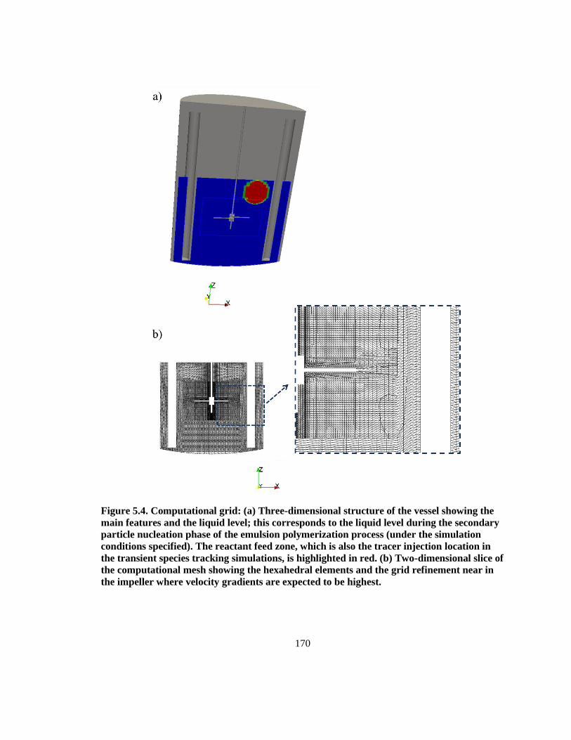
170
Figure 5.4. Computational grid: (a) Three-dimensional structure of the vessel showing the
main features and the liquid level; this corresponds to the liquid level during the secondary
particle nucleation phase of the emulsion polymerization process (under the simulation
conditions specified). The reactant feed zone, which is also the tracer injection location in
the transient species tracking simulations, is highlighted in red. (b) Two-dimensional slice of
the computational mesh showing the hexahedral elements and the grid refinement near in
the impeller where velocity gradients are expected to be highest.
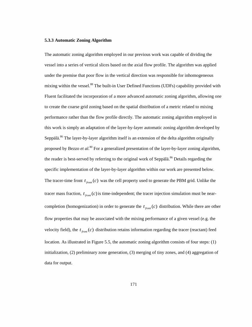
171
5.3.3 Automatic Zoning Algorithm
The automatic zoning algorithm employed in our previous work was capable of dividing the
vessel into a series of vertical slices based on the axial flow profile. The algorithm was applied
under the premise that poor flow in the vertical direction was responsible for inhomogeneous
mixing within the vessel.88
The built-in User Defined Functions (UDFs) capability provided with
Fluent facilitated the incorporation of a more advanced automatic zoning algorithm, allowing one
to create the coarse grid zoning based on the spatial distribution of a metric related to mixing
performance rather than the flow profile directly. The automatic zoning algorithm employed in
this work is simply an adaptation of the layer-by-layer automatic zoning algorithm developed by
Seppälä.86
The layer-by-layer algorithm itself is an extension of the delta algorithm originally
proposed by Bezzo et al.80
For a generalized presentation of the layer-by-layer zoning algorithm,
the reader is best-served by referring to the original work of Seppälä.86
Details regarding the
specific implementation of the layer-by-layer algorithm within our work are presented below.
The tracer-time front ( )frontt c was the cell property used to generate the PBM grid. Unlike the
tracer mass fraction, ( )frontt c is time-independent; the tracer injection simulation must be near-
completion (homogenization) in order to generate the ( )frontt c distribution. While there are other
flow properties that may be associated with the mixing performance of a given vessel (e.g. the
velocity field), the ( )frontt c distribution retains information regarding the tracer (reactant) feed
location. As illustrated in Figure 5.5, the automatic zoning algorithm consists of four steps: (1)
initialization, (2) preliminary zone generation, (3) merging of tiny zones, and (4) aggregation of
data for output.
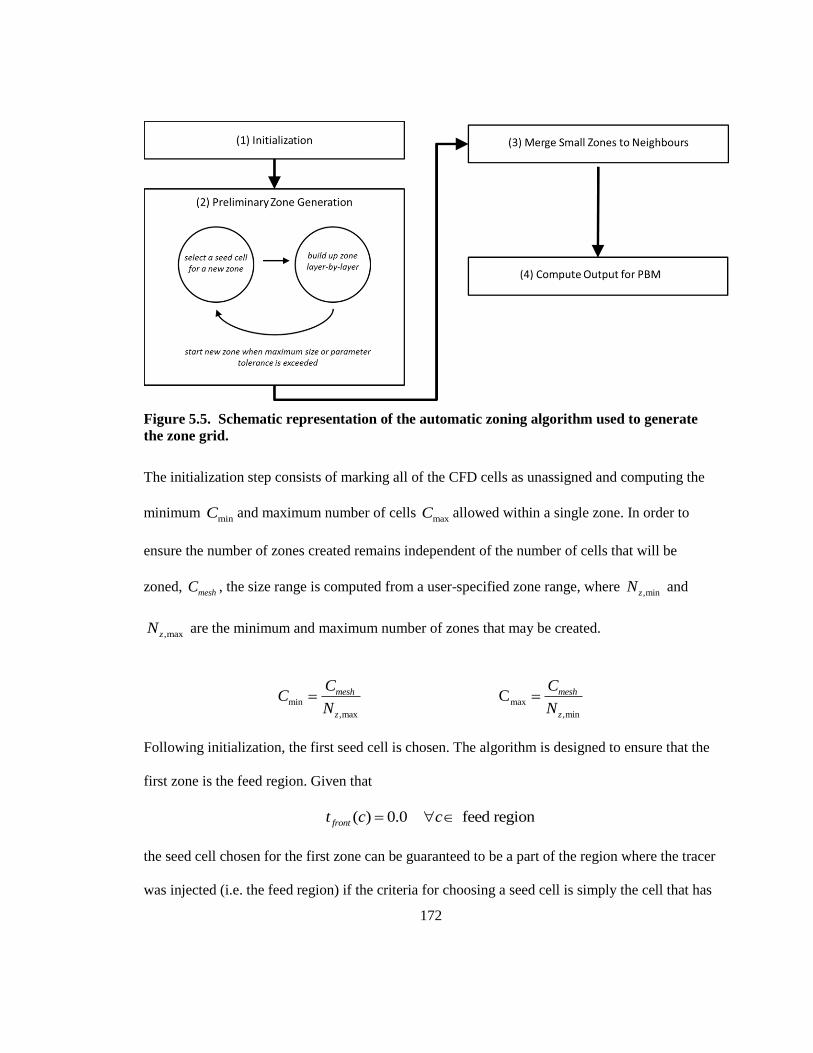
172
Figure 5.5. Schematic representation of the automatic zoning algorithm used to generate
the zone grid.
The initialization step consists of marking all of the CFD cells as unassigned and computing the
minimum minC and maximum number of cells
maxC allowed within a single zone. In order to
ensure the number of zones created remains independent of the number of cells that will be
zoned, meshC , the size range is computed from a user-specified zone range, where
,minzN and
,maxzN are the minimum and maximum number of zones that may be created.
min max
,max ,min
Cmesh mesh
z z
C CC
N N
Following initialization, the first seed cell is chosen. The algorithm is designed to ensure that the
first zone is the feed region. Given that
( ) 0.0 feed regionfrontt c c
the seed cell chosen for the first zone can be guaranteed to be a part of the region where the tracer
was injected (i.e. the feed region) if the criteria for choosing a seed cell is simply the cell that has

173
minimal value of ( )frontt c . Once a seed cell is chosen, the tolerance ( )seedc for the zone is
computed. The following function will provide reasonable ( )seedc values under most
circumstances:
min 0( ) max , ( )seed front seedc a t c (5.86)
Setting 0 frontt will ensure that ( )seedc will approach zero as ( )front seedt c approaches
frontt .
A minimum tolerance min is specified to ensure that does not cross a minimum threshold.
If the frequency distribution of ( )frontt c is not a normal aboutfrontt ,
0 may be set to another
value, such as the median or mode of the frequency distribution. The second adjustable
parameter a can be used to adjust the order-of-magnitude of the computed tolerance.
Once the seed cell has been selected and the zone tolerance parameter has been computed, the
zone is grown through the addition of eligible neighbouring cells. An eligible neighbouring cell is
defined as a cell that shares at least one face with a cell that belongs to the zone that is being
created. In the layer-by-layer algorithm LBL , all unattached neighbouring cells are added to the
zone as a layer as shown schematically in Figure 5.6. After the addition of each layer, the range
of frontt , , is computed:
,max ,mini i
front frontc z c zt t
(5.87)
If , the zone is said to homogeneous in frontt within the computed tolerance and another
layer is added. If the tolerance is exceeded, the construction of the zone is completed and a new
zone is started. There are a number of additional rules specified to control zone construction. A
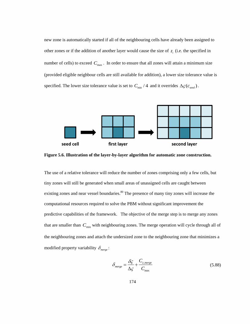
174
new zone is automatically started if all of the neighbouring cells have already been assigned to
other zones or if the addition of another layer would cause the size of iz (i.e. the specified in
number of cells) to exceed maxC . In order to ensure that all zones will attain a minimum size
(provided eligible neighbour cells are still available for addition), a lower size tolerance value is
specified. The lower size tolerance value is set to min / 4C and it overrides ( )seedc .
Figure 5.6. Illustration of the layer-by-layer algorithm for automatic zone construction.
The use of a relative tolerance will reduce the number of zones comprising only a few cells, but
tiny zones will still be generated when small areas of unassigned cells are caught between
existing zones and near vessel boundaries.80
The presence of many tiny zones will increase the
computational resources required to solve the PBM without significant improvement the
predictive capabilities of the framework. The objective of the merge step is to merge any zones
that are smaller than minC with neighbouring zones. The merge operation will cycle through all of
the neighbouring zones and attach the undersized zone to the neighbouring zone that minimizes a
modified property variability merge :
,
max
z merge
merge
C
C
(5.88)
175
To account for the fact that best potential merger (i.e. the merge operation that minimizes the
aggregate variability ) may result in a zone that is larger than maxC , the merge is penalized
rather than restricted outright. Some merge operations will result in the creation zones that are
still undersized; these zones will be continually merged with neighbouring zones until all zones
are larger than the computed minimum size, minC .
Once the merge operation is complete, the output files responsible for passing data on to the PBM
are created. The volume and connectivity of each zone is recorded, along with the interzonal flow
rates and mean shear rate in each zone. The volumetric rate of flow exchanged between
interconnected zones is computed by looping through all cell faces in the domain. Faces that do
not fall on an interface between cells do not contribute to the interzonal flow rate array. If a cell
does fall on an interface between two zones, the direction of the flow will determine which array
entry the flow will contribute to. For example, the interface ,i jI is comprised of a number of cell
faces. The flow across some faces will be from zone i to zone j , while the flow across other
faces will be from zone j to zone i . Thus the flow rate across the interface is split into two
components: ,i jq and
,j iq , where ,i jq is the sum of flow from all the faces on the interface
,i jI
for which the flow direction is from zone i to zone j ; if the flow direction is instead from zone
j to zone i , the flow is added to ,j iq . Note that for zone i , the total rate of flow exiting the zone
is ,
,
i j
j j i
q
, while the total rate of flow entering the zone is ,
,
j i
j j i
q
. Given that the flow field is
computed at steady-state,
, ,
, ,
0i j j i
j j i j j i
q q
176
If the net rate of flow is not zero (within a small tolerance), the PBM may suffer from
convergence issues, so the algorithm will check the net discrepancy between total flow entering
all zones and total flow exiting all zones.
The shear rate magnitude used to compute fluid viscosity in the PBM is a scalar quantity. The
average shear rate for each zone c is computed as a volume average as follows:
c cc z
z
z
v
V
(5.89)
where cv is the volume of an individual CFD mesh cell.
5.4 Results & Discussion
All simulations were performed on a desktop computer equipped with an Intel Core 2 Quad 6600
@ 2.40 GHz and 6.0 GB of RAM. Approximate computation times for each framework
component were as follows:
CFD flow field simulation ~ 1.5 hours
CFD tracer dispersion simulation ~ 0.25 to 2.5 hours (dependent on vessel scale)
automatic zoning algorithm ~ 3 minutes
multi-zonal PBM ~ 2.5 to 10 hours for 100 zones (dependent on vessel scale)
Total simulation time per case ranged between 4.5 hours and 15 hours, with the larger reactor
scales requiring more computation time per case. The simulation time required for tracer dispersal
simulations was proportional to the number of time steps required to completely disperse the
tracer. PBM simulation time was dependent on the occurrence of particle nucleation and particle
177
coagulation, as the time step size was reduced while these events are occurring at high rates
during the reaction.
5.4.1 Blending Simulations & Zone Generation
In generating the PBM mesh, the objective was to divide the PBM into a series of interconnected
zones. While the contents of each individual zone are assumed to be homogeneous, the
arrangement of zones is designed to capture the effect of vessel inhomogeneity on the evolution
of PSD within the PBM. The feed zone is the only zone on the PBM grid that is both fixed in size
and shape; this step was taken in order to ensure that the concentration of species entering the
first zone is independent of vessel scale. This approximates an assumption that the diameter of the
feed dip pipe would increase in proportion to the tank diameter, but it would be possible to
examine other scenarios.
The PBM grid is generated using a transient inert tracer species balance simulation. As the tracer
is dispersed through the vessel, its local mass fraction will continue to evolve until it reaches a
state of uniform concentration throughout the entire vessel. The mixing time can be expressed
quantitatively using a number of metrics. In this work, the blend time is defined as the time taken
to reduce the maximum variation in tracer concentration by 95% from its initial value. The
variation in tracer concentration can be expressed in a dimensionless, bounded form as follows:
max max
max
( 0) ( )( )
( 0)
t tU t
t
(5.90)
where max ( )t is computed from the distribution of tracer mass fraction (
trC ) throughout the
vessel.
178
max ,max ,min( ) max ,tr tr tr trt C C C C (5.91)
By definition, 0 0.0U t and ( ) 1.0U t when the system is fully-homogeneous. The
blend time blendt is defined as the time required for ( )U t to reach 0.95. The mixing curves for
the set of simulations where the reactor was scaled-up maintaining constant P/V are plotted in
Figure 5.7. The simulation blend times can be read off of Figure 5.7 by observing where the
mixing curves intersect the upper horizontal axis (the ordinate). The blend time data for all
simulations is summarized graphically in Figure 5.8. The blending time data presented in Figure
5.7 suggests that if the vessel is scaled-up maintaining a constant P/V ratio, blend time increases
from approximately 6.5 seconds at the 1-L scale, to 11 seconds at the 100-L scale and, finally, to
29.5 seconds at the 10-m3 scale. It is noted that blend time is expected to increase by roughly a
factor of 2.7 for an increase in vessel volume by a factor of 100.87
The increase in blend time
from the 100 L scale to the 10-m3 scale closely matches expectation, while the increase in blend
time between the 1-L and 100-L vessel scales is less than expected. This discrepancy may be
partially explained by the fact that the 1 L vessel is operating at a Reynolds number close to the
threshold of 104 that is typically used to characterize the turbulent regime
4
Re( 2.1 10 )N and
thus is not operating in the fully-developed region. Examination of Figure 5.8 reveals that when
the 1 L vessel is scaled up to 100 L with the objective of maintaining a constant blend time, the
computed blend time actually drops from 6.5 seconds to 4.2 seconds. The scale-up heuristics
were developed under the assumption that flow at both scales is fully-turbulent, so the drop in
blend time indicates that the 1 L vessel is operating in the transitional-regime. However the
discrepancy between blend times when the vessel is scaled up based on constant TQ/V is also
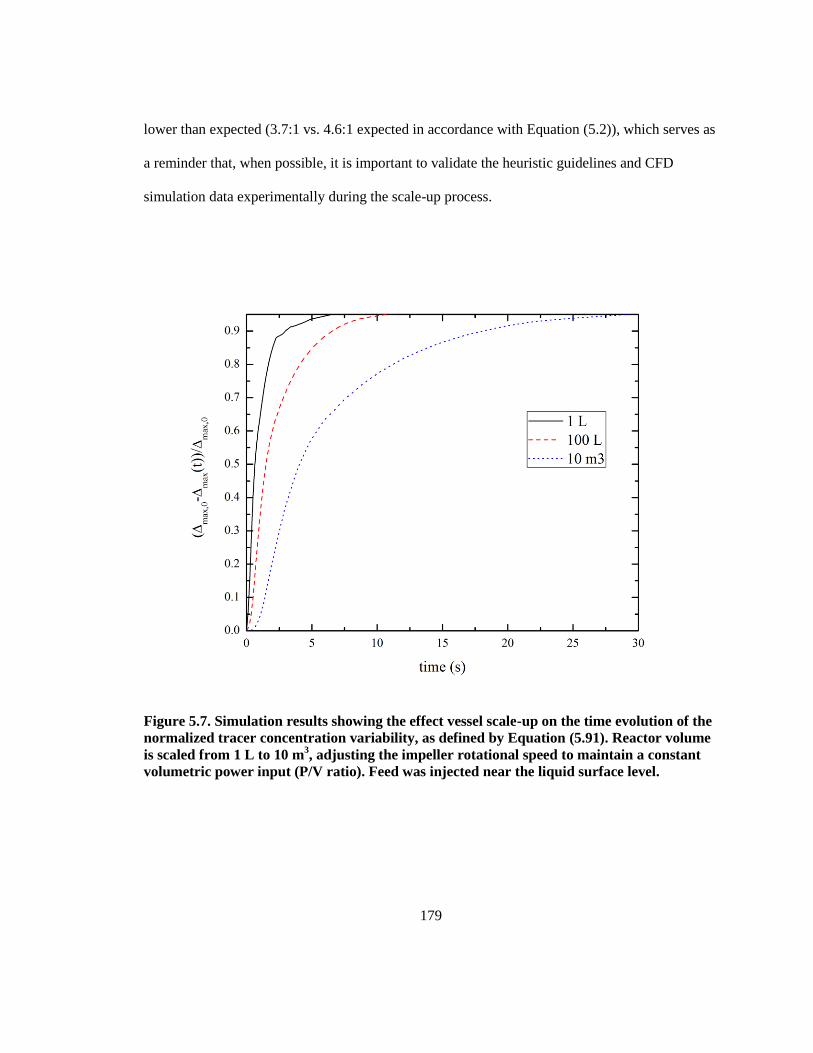
179
lower than expected (3.7:1 vs. 4.6:1 expected in accordance with Equation (5.2)), which serves as
a reminder that, when possible, it is important to validate the heuristic guidelines and CFD
simulation data experimentally during the scale-up process.
Figure 5.7. Simulation results showing the effect vessel scale-up on the time evolution of the
normalized tracer concentration variability, as defined by Equation (5.91). Reactor volume
is scaled from 1 L to 10 m3, adjusting the impeller rotational speed to maintain a constant
volumetric power input (P/V ratio). Feed was injected near the liquid surface level.
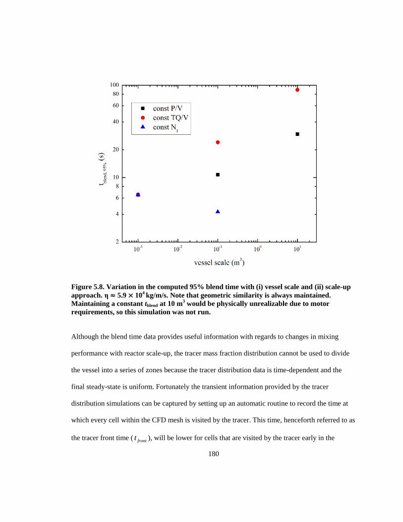
180
Figure 5.8. Variation in the computed 95% blend time with (i) vessel scale and (ii) scale-up
approach. η ≈ 5.9 × 10⁴
kg/m/s. Note that geometric similarity is always maintained.
Maintaining a constant tblend at 10 m3 would be physically unrealizable due to motor
requirements, so this simulation was not run.
Although the blend time data provides useful information with regards to changes in mixing
performance with reactor scale-up, the tracer mass fraction distribution cannot be used to divide
the vessel into a series of zones because the tracer distribution data is time-dependent and the
final steady-state is uniform. Fortunately the transient information provided by the tracer
distribution simulations can be captured by setting up an automatic routine to record the time at
which every cell within the CFD mesh is visited by the tracer. This time, henceforth referred to as
the tracer front time (frontt ), will be lower for cells that are visited by the tracer early in the
181
simulation and highest for the cells that are visited last. The cell is assigned a frontt value
corresponding to the earliest time at which the tracer mass fraction inside the cell equals or
exceeds a minimum threshold. The minimum threshold is chosen such that every cell will have
been assigned a frontt value by the time the simulation reaches a steady state. The largest value at
which this is possible equals trC , the volume-averaged tracer mass fraction. For this reason, the
maximum value of frontt in the domain is the time required to completely distribute the tracer
throughout the vessel or the 100% blend time.
At the conditions specified, all of the CFD mesh cells received tracer, although there were a few
(< 10) cells where frontt was around five times the 95% blend time. The distribution of tracer to a
few segregated cells within the vessel domain often requires a large number of additional time
steps, so the tracer mass fraction threshold can be reduced to reduce computation time. In this
work, the threshold was set equal to /10trC . The reduction in the tracer mass fraction threshold
is reasonable as it is the relative shape of the frontt distribution (i.e. the histogram), not the
absolute values within the frontt distribution that determine the corresponding zone network.
Note that if fluid viscosity is very high and mixing is poor, a large proportion of the domain may
be completely-segregated. These segregated cells should be aggregated into their own separate
zones in order to capture the impact of the segregation within the framework.
Figure 5.9 shows the evolution of both the flow field and the tracer front distribution with scale
(maintaining a constant P/V ratio) along a vertical slice at the center of the vessel. The general
182
shape of the flow pattern observed across all three scales is very similar, although the volume-
averaged velocity magnitude increases as the reactor is scaled-up. The similarity of the flow
patterns is expected as the smallest vessel is characterized by a Reynolds numbers of 1 × 10⁴ and
flow is said to be fully-turbulent for Re > 1 × 10⁴. The increase in blend time with reactor scale is
apparent when looking at the tracer front distributions; the 10 m3 tank features a sizeable area
near the bottom of the tank where mixing is slow compared to small scale vessels. The
asymmetry in the tracer front-time distribution in the upper region of the tank arises from the off-
center feed location.
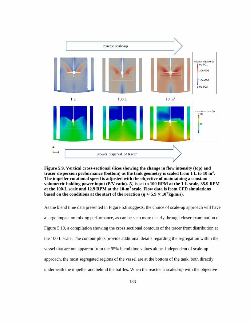
183
Figure 5.9. Vertical cross-sectional slices showing the change in flow intensity (top) and
tracer dispersion performance (bottom) as the tank geometry is scaled from 1 L to 10 m3.
The impeller rotational speed is adjusted with the objective of maintaining a constant
volumetric holding power input (P/V ratio). NI is set to 100 RPM at the 1-L scale, 35.9 RPM
at the 100-L scale and 12.9 RPM at the 10-m3 scale. Flow data is from CFD simulations
based on the conditions at the start of the reaction (η ≈ 5.9 × 10⁴ kg/m/s).
As the blend time data presented in Figure 5.8 suggests, the choice of scale-up approach will have
a large impact on mixing performance, as can be seen more clearly through closer examination of
Figure 5.10, a compilation showing the cross sectional contours of the tracer front distribution at
the 100 L scale. The contour plots provide additional details regarding the segregation within the
vessel that are not apparent from the 95% blend time values alone. Independent of scale-up
approach, the most segregated regions of the vessel are at the bottom of the tank, both directly
underneath the impeller and behind the baffles. When the reactor is scaled-up with the objective
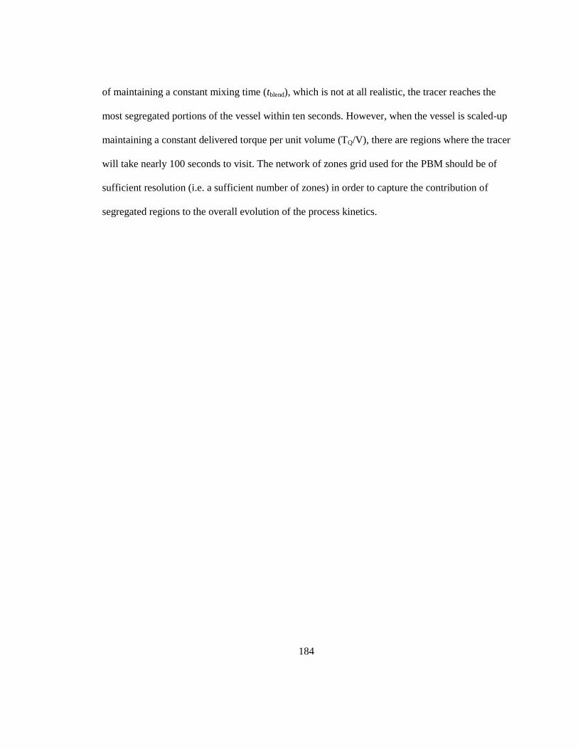
184
of maintaining a constant mixing time (tblend), which is not at all realistic, the tracer reaches the
most segregated portions of the vessel within ten seconds. However, when the vessel is scaled-up
maintaining a constant delivered torque per unit volume (TQ/V), there are regions where the tracer
will take nearly 100 seconds to visit. The network of zones grid used for the PBM should be of
sufficient resolution (i.e. a sufficient number of zones) in order to capture the contribution of
segregated regions to the overall evolution of the process kinetics.
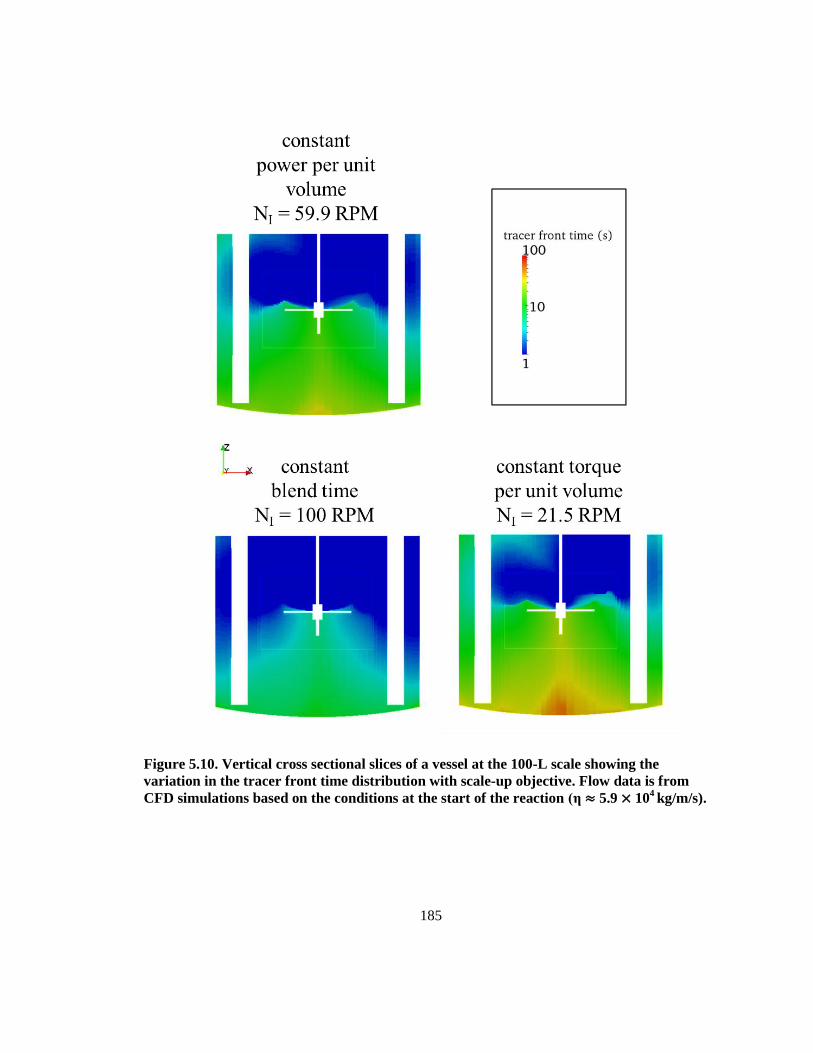
185
Figure 5.10. Vertical cross sectional slices of a vessel at the 100-L scale showing the
variation in the tracer front time distribution with scale-up objective. Flow data is from
CFD simulations based on the conditions at the start of the reaction (η ≈ 5.9 × 10⁴
kg/m/s).

186
Once the frontt distribution is obtained, the zone grid is generated using the layer-by-layer zoning
algorithm. The algorithm was designed with the potential of employing more than one property to
build the zone structure, but the tracer front time ( )frontt was the sole property used in this work.
The tolerances used to zone the reactor based on the distribution of frontt values were as follows:
min 00.35 0.080 fronta t
A typical zone distribution is shown in Figure 5.11. The computation time required to zone one
CFD domain is around 60 seconds; the relatively short computation time is one of the strengths of
the layer-by-layer algorithm.86
The number of zones generated is not controlled directly; rather
the range is specified by adjusting ,minzN and
,maxzN , the minimum and maximum number of
cells per zone, respectively. A grid independence test, based on the PSD obtained in at 10-m3
scale (the most computationally-intensive scenario due to extensive concentration gradients) after
1.75 h was performed to determine the number of zones required within the population balance
model to render the simulation output grid independent. The results indicated that approximately
100 zones were required to achieve zone grid independence and this was achieved by setting
,minzN and ,maxzN to 80 and 150, respectively. In the simulations presented in this work, the
number of zones generated varied between 99 and 102.
Closer examination of Figure 5.11 reveals that the zones generated with the layer-by-layer
algorithm are visually blocky and do not match the contours of tracer front time exactly. The
blocky shape of the zones is characteristic of the layer-by-layer zoning algorithm. The final shape
of the zones can be designed to closely follow the contours of the property data sets used to
generate the zones by reducing the tolerance terms used to determine whether to reject an
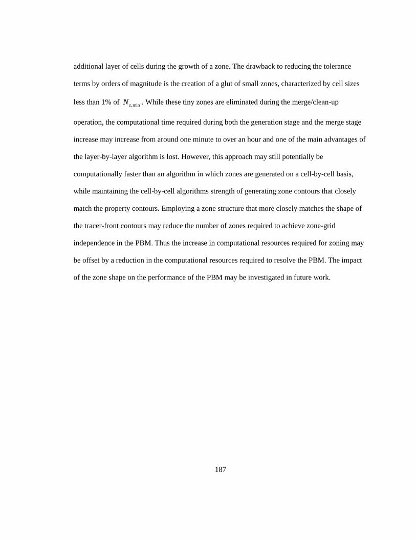
187
additional layer of cells during the growth of a zone. The drawback to reducing the tolerance
terms by orders of magnitude is the creation of a glut of small zones, characterized by cell sizes
less than 1% of ,minzN . While these tiny zones are eliminated during the merge/clean-up
operation, the computational time required during both the generation stage and the merge stage
increase may increase from around one minute to over an hour and one of the main advantages of
the layer-by-layer algorithm is lost. However, this approach may still potentially be
computationally faster than an algorithm in which zones are generated on a cell-by-cell basis,
while maintaining the cell-by-cell algorithms strength of generating zone contours that closely
match the property contours. Employing a zone structure that more closely matches the shape of
the tracer-front contours may reduce the number of zones required to achieve zone-grid
independence in the PBM. Thus the increase in computational resources required for zoning may
be offset by a reduction in the computational resources required to resolve the PBM. The impact
of the zone shape on the performance of the PBM may be investigated in future work.
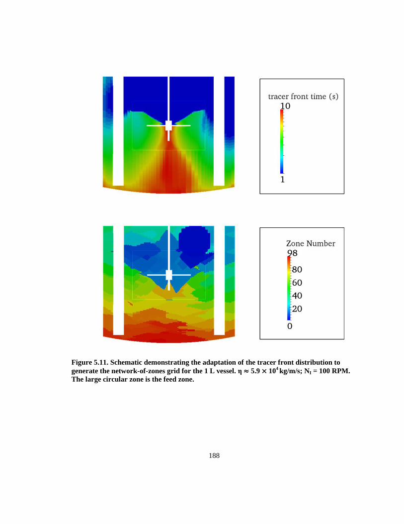
188
Figure 5.11. Schematic demonstrating the adaptation of the tracer front distribution to
generate the network-of-zones grid for the 1 L vessel. η ≈ 5.9 × 10⁴ kg/m/s; NI = 100 RPM.
The large circular zone is the feed zone.
189
5.4.2 Framework Predictions
A primary objective of this work was to demonstrate the use of a computational framework for
predicting how changes to the macro-mixing length, inherent to process scale-up, may affect the
properties of the final polystyrene latex. The key property of focus in this work is the PSD. As
mentioned in the introduction, changes in the PSD will affect the ease with which the product can
be processed, the productivity (via the achievable solids concentration), and the performance in
end-use applications such as film formation time and the permeability of the film. The inherent
complexity of the emulsion polymerization process dictates that further advances in the
framework will be beneficial, potentially providing meaningful guidance towards a larger scope
of potential issues, such as heat transfer considerations, production yield and product molecular
weight(s).
The main objective of scale-up is to design a large scale mixing system that achieves the same
mixing quality as a laboratory tank.87
In very large reactors, achieving a similar mixing quality
may be impossible, in which case the objective is to understand how changes in the length and
time scale influence product quality, so that conditions at the large scale may be altered in order
to overcome these differences. In the production of polymer latexes, particularly high solid
content latexes, achieving the correct proportion of large particles and small particles is necessary
in order to meet productivity and quality objectives.30
One of the most important objectives in the
production of concentrated polymer latexes is the timely dispersion of reactants throughout the
vessel. The associated scale-up method towards achieving this objective is to maintain a
consistent blend time across reactor scales. If the flow regime is fixed (i.e. both the laboratory and
190
commercial vessels rely on turbulent mixing), the process blend time is inversely proportional to
the impeller rotational speed.87
Maintaining a constant blend time (tblend) is generally not feasible
due to the increased energy and torque requirements associated with maintaining a constant
impeller rotational speed during scale-up. For a process utilizing a pitched-blade turbine agitation
system within the turbulent regime, the scale-up from a 1 L laboratory vessel to a 10 m3
commercial vessel requires approximately 450 times the amount of holding power per unit
volume and the gearbox would be have to deliver roughly 3000 times the amount of torque per
unit volume of latex being produced. Conversely, the most pragmatic scale-up approach,
assuming that motor size will be restricted at the largest scales, is to maintain a constant delivered
torque per unit volume (TQ/V). In between these two extremes lies the recommended “first-
guess” approach:10
delivery of a constant holding power per unit volume (P/V) across a wide
range of vessel scales.
CFD simulation, when used in isolation, can provide helpful information to process engineers. It
has already been shown that predicted blend time will increase from 6.5s to around 90s (an
increase by a factor of 14) when scaling up from 1 L to 10 m3 when the impeller rotational rate
was adjusted to maintain constant TQ/V. This is less than the change predicted by classical
heuristics alone, whereby blend time is expected to increase by a factor of 21.5, and it can be
attributed to a transition from mostly-turbulent to fully-turbulent mixing. The advantage of
incorporating CFD simulation into a framework containing a population balance model lies in
being able to directly predict the impact of different scale-up approaches on final product
properties, a more direct indicator of productivity than process blend time.
191
As stated above, one of the current restrictions of the framework presented in this work is the
fixed arrangement of the network-of-zones. Many latex products are produced in semi-batch
process, whereby the liquid height will change over the course of reaction. The mixing
performance of a reactor may change as the liquid level rises. In a reactor agitated with a single
impeller, mixing performance is known to be very poor if the aspect ratio (the ratio of liquid level
to vessel diameter) increases beyond 1.5.87
The network of zones generated at a low liquid level
will differ from the network of zones generated at a high liquid level, as can be seen in Figure
5.12. The general shape of the zones in the lower region of the tank remains the same if the feed
location does not change with liquid level (e.g. using a feed pipe to ensure the feed is introduced
near the impeller), as the flow profile in the bottom of the tank maintains a similar shape.
However, the size of the automatically-generated zones will increase with liquid height unless the
zoning parameters,,minzN and
,maxzN are adjusted in proportion with the relative change in the
liquid level.
The most pragmatic solution for dealing with a variable liquid level (with a fixed feed location)
may be to generate the zones using the maximum liquid level. The upper region zones could be
initially specified as empty and the flow-exchange information could be updated periodically to
account for the changing location of the liquid surface. The case where the feed region changes
with liquid level (e.g. a surface feed) is more challenging, as the time required for reactants to
spread to the lower regions of the tank will increase as the liquid level rises. The network-of-
zones grid would need to be reshaped periodically, requiring the aggregation and redistribution of
data as the location and shapes of the individual zones would change. There is no guarantee that
the PBM predictions will remain accurate as multiple aggregation and redistribution operations
192
are carried-out over the course of a full simulation, unless the resolution of the zone grid is
increased substantially.
Fortunately the framework can produce meaningful predictions for semi-batch processes if the
kinetic events that are affected by mixing performance are restricted to short time periods, over
which liquid level can be assumed to be constant. In the production of a bimodal polystyrene
latex, it would not be unreasonable to propose that the in situ generation of the secondary particle
population is the production step which is most strongly affected by the mixing performance of
the reactor. A change in the number density of small particles produced will subsequently affect
the growth of both the small and large particles, leading to changes in the diameter ratio between
and volume proportion of small particles to large particles. Concurrently it is important to
demonstrate that the last step in the process, the growth of both populations, is not restricted by
the mixing capabilities of the vessel at the largest scale.
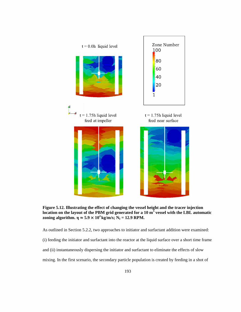
193
Figure 5.12. Illustrating the effect of changing the vessel height and the tracer injection
location on the layout of the PBM grid generated for a 10 m3 vessel with the LBL automatic
zoning algorithm. η ≈ 5.9 × 10⁴ kg/m/s; NI = 12.9 RPM.
As outlined in Section 5.2.2, two approaches to initiator and surfactant addition were examined:
(i) feeding the initiator and surfactant into the reactor at the liquid surface over a short time frame
and (ii) instantaneously dispersing the initiator and surfactant to eliminate the effects of slow
mixing. In the first scenario, the secondary particle population is created by feeding in a shot of
194
surfactant and initiator over a period of approximately five minutes. The inability of the reactor to
instantaneously disperse the reactants results in a concentration gradient, with the concentration
of surfactant and initiator being highest in the feed zone. This has two effects. The first effect is a
high local micelle concentration, leading to an increased rate of micellar nucleation. The second
effect is an increase in the local ionic strength which affects particle stability and thus the rate of
particle coagulation. The localized concentration gradients during this short nucleation phase will
have a large impact on the PSD of the final product, as can be seen via examination of Figure
5.13. There are two trends to note as the vessel is scaled-up using the constant P/V criterion. The
first trend is the widening of the large mode, a trend that asserts itself even when departing from
perfect mixing to the 1-L scale. The probable cause of this widening is rapid particle coagulation
within the reactor zones where local ion concentration exceeds a critical coagulation
concentration (CCC). At the 1-L scale and 100-L scale, the peak of the large mode remains
around 340 nm in diameter. This suggests that the small particles, as they‟re formed via micellar
nucleation, are rapidly coagulating with the large particles and with other small particles. Large
particles, due to their lower number concentration are much less likely to collide and coagulate
with other large particles.99
The second scale-up effect seen in Figure 5.13 is the change in the peak diameters of both modes,
which is only seen at the 10-m3 scale. The large particle mode drops from 340 nm to around 310
nm in diameter, while the small particle mode increases from roughly 15 nm to 25 nm in
diameter. The mass fraction of small particles is also much higher at the 10-m3 scale compared to
all others. The rate of particle nucleation appears to be higher at the 10-m3 scale; the fact that the
effect is not seen at the 100-L scale suggests that the time scale of rapid particle coagulation may
195
be faster than the time scale of micellar nucleation (i.e. if the reactor was scaled-up gradually, one
would observe issues with regards to rapid particle coagulation before observing changes with
regards to particle nucleation). However, examining the final Np values (refer to Figure 5.14), the
number of particles actually decreases from approximately 2.2 × 10²²
m-3
at the 1-L and 100-L
scales to 1.4 × 10²²
m-3
at the 10-m3 scale. The enhanced rate of particle nucleation has a
secondary effect on the final PSD arising from the competitive growth between the two sets of
particles. The cross-over diameter between zero-one and pseudo-bulk for styrene is around 110
nm, such that the free radicals are compartmentalized within the small particles, but not within
the large particles. The growth rate of the large particles is proportional to the aggregate volume
of the large particle population while the growth of the small particles is proportional to their
number concentration. The small particles will continue to grow at a constant rate,
notwithstanding ongoing particle coagulation, while the growth of large particles tends to
accelerate as they grow in volume. The enhanced nucleation rate of small particles leads to a
larger proportion of the polymerization occurring within the smaller particles and slower growth
in the mean volume of the large particle population. This reduces the transient divergence in the
competitive growth rate between the two populations, which results in a narrower diameter ratio
between the large mode and small mode in the final product. At the 10-m3 scale, the large particle
PSD is wider and has a large tail skewed towards a higher diameter, suggesting an increased rate
of large particles coagulating with other large particles.
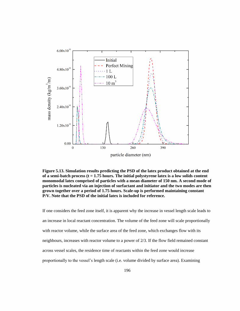
196
Figure 5.13. Simulation results predicting the PSD of the latex product obtained at the end
of a semi-batch process (t = 1.75 hours. The initial polystyrene latex is a low solids content
monomodal latex comprised of particles with a mean diameter of 150 nm. A second mode of
particles is nucleated via an injection of surfactant and initiator and the two modes are then
grown together over a period of 1.75 hours. Scale-up is performed maintaining constant
P/V. Note that the PSD of the initial latex is included for reference.
If one considers the feed zone itself, it is apparent why the increase in vessel length scale leads to
an increase in local reactant concentration. The volume of the feed zone will scale proportionally
with reactor volume, while the surface area of the feed zone, which exchanges flow with its
neighbours, increases with reactor volume to a power of 2/3. If the flow field remained constant
across vessel scales, the residence time of reactants within the feed zone would increase
proportionally to the vessel‟s length scale (i.e. volume divided by surface area). Examining
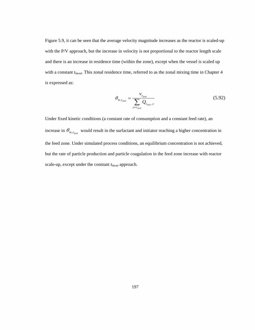
197
Figure 5.9, it can be seen that the average velocity magnitude increases as the reactor is scaled-up
with the P/V approach, but the increase in velocity is not proportional to the reactor length scale
and there is an increase in residence time (within the zone), except when the vessel is scaled up
with a constant tblend. This zonal residence time, referred to as the zonal mixing time in Chapter 4
is expressed as:
,
,
feed
feed
feed
feed
z
m z
z y
y z
v
Q
(5.92)
Under fixed kinetic conditions (a constant rate of consumption and a constant feed rate), an
increase in , feedm z would result in the surfactant and initiator reaching a higher concentration in
the feed zone. Under simulated process conditions, an equilibrium concentration is not achieved,
but the rate of particle production and particle coagulation in the feed zone increase with reactor
scale-up, except under the constant tblend approach.
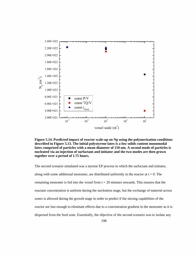
198
Figure 5.14. Predicted impact of reactor scale-up on Np using the polymerization conditions
described in Figure 5.13. The initial polystyrene latex is a low solids content monomodal
latex comprised of particles with a mean diameter of 150 nm. A second mode of particles is
nucleated via an injection of surfactant and initiator and the two modes are then grown
together over a period of 1.75 hours.
The second scenario simulated was a styrene EP process in which the surfactant and initiator,
along with some additional monomer, are distributed uniformly in the reactor at t = 0. The
remaining monomer is fed into the vessel from t = 20 minutes onwards. This ensures that the
reactant concentration is uniform during the nucleation stage, but the exchange of material across
zones is allowed during the growth stage in order to predict if the mixing capabilities of the
reactor are fast enough to eliminate effects due to a concentration gradient in the monomer as it is
dispersed from the feed zone. Essentially, the objective of the second scenario was to isolate any
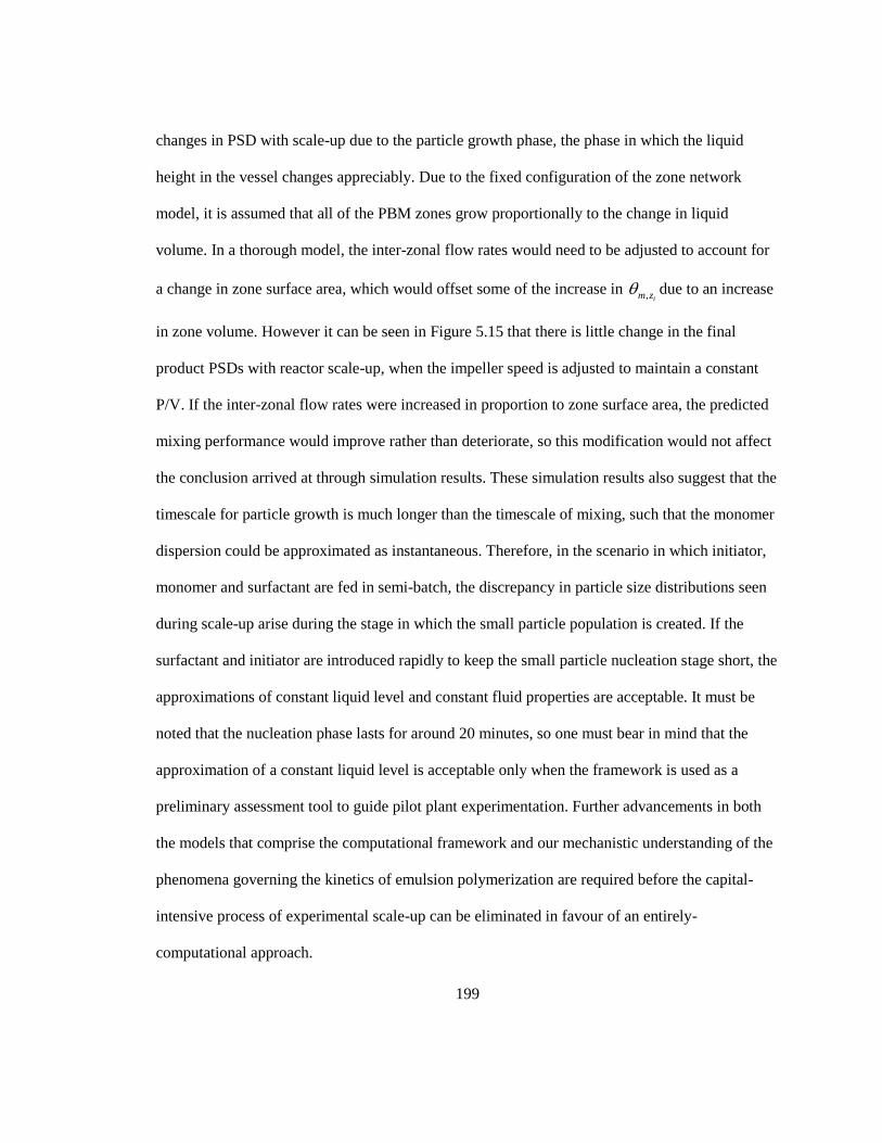
199
changes in PSD with scale-up due to the particle growth phase, the phase in which the liquid
height in the vessel changes appreciably. Due to the fixed configuration of the zone network
model, it is assumed that all of the PBM zones grow proportionally to the change in liquid
volume. In a thorough model, the inter-zonal flow rates would need to be adjusted to account for
a change in zone surface area, which would offset some of the increase in , im z due to an increase
in zone volume. However it can be seen in Figure 5.15 that there is little change in the final
product PSDs with reactor scale-up, when the impeller speed is adjusted to maintain a constant
P/V. If the inter-zonal flow rates were increased in proportion to zone surface area, the predicted
mixing performance would improve rather than deteriorate, so this modification would not affect
the conclusion arrived at through simulation results. These simulation results also suggest that the
timescale for particle growth is much longer than the timescale of mixing, such that the monomer
dispersion could be approximated as instantaneous. Therefore, in the scenario in which initiator,
monomer and surfactant are fed in semi-batch, the discrepancy in particle size distributions seen
during scale-up arise during the stage in which the small particle population is created. If the
surfactant and initiator are introduced rapidly to keep the small particle nucleation stage short, the
approximations of constant liquid level and constant fluid properties are acceptable. It must be
noted that the nucleation phase lasts for around 20 minutes, so one must bear in mind that the
approximation of a constant liquid level is acceptable only when the framework is used as a
preliminary assessment tool to guide pilot plant experimentation. Further advancements in both
the models that comprise the computational framework and our mechanistic understanding of the
phenomena governing the kinetics of emulsion polymerization are required before the capital-
intensive process of experimental scale-up can be eliminated in favour of an entirely-
computational approach.
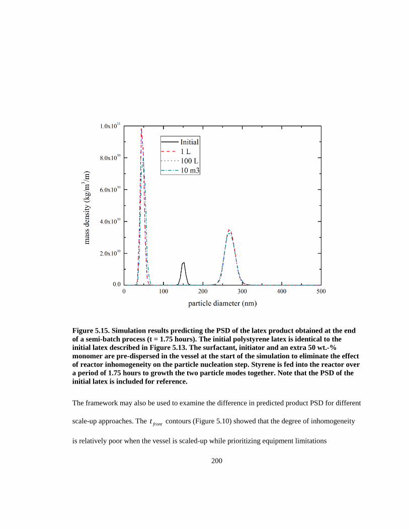
200
Figure 5.15. Simulation results predicting the PSD of the latex product obtained at the end
of a semi-batch process (t = 1.75 hours). The initial polystyrene latex is identical to the
initial latex described in Figure 5.13. The surfactant, initiator and an extra 50 wt.-%
monomer are pre-dispersed in the vessel at the start of the simulation to eliminate the effect
of reactor inhomogeneity on the particle nucleation step. Styrene is fed into the reactor over
a period of 1.75 hours to growth the two particle modes together. Note that the PSD of the
initial latex is included for reference.
The framework may also be used to examine the difference in predicted product PSD for different
scale-up approaches. The frontt contours (Figure 5.10) showed that the degree of inhomogeneity
is relatively poor when the vessel is scaled-up while prioritizing equipment limitations
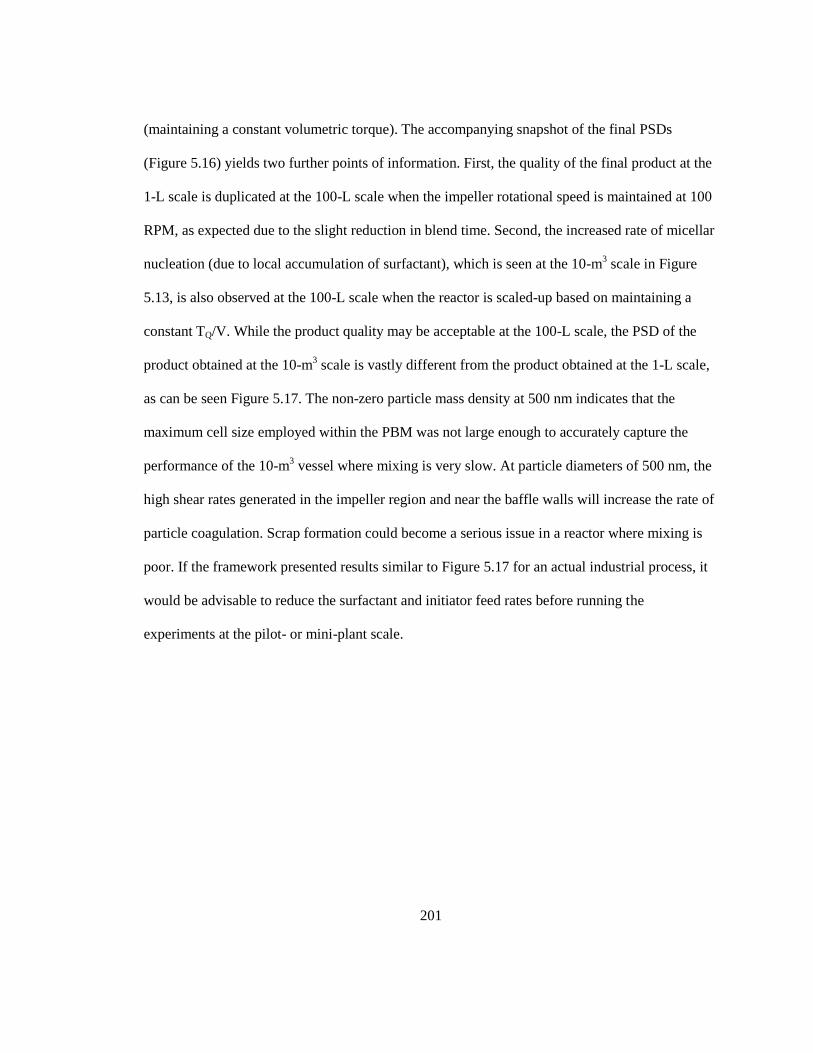
201
(maintaining a constant volumetric torque). The accompanying snapshot of the final PSDs
(Figure 5.16) yields two further points of information. First, the quality of the final product at the
1-L scale is duplicated at the 100-L scale when the impeller rotational speed is maintained at 100
RPM, as expected due to the slight reduction in blend time. Second, the increased rate of micellar
nucleation (due to local accumulation of surfactant), which is seen at the 10-m3 scale in Figure
5.13, is also observed at the 100-L scale when the reactor is scaled-up based on maintaining a
constant TQ/V. While the product quality may be acceptable at the 100-L scale, the PSD of the
product obtained at the 10-m3 scale is vastly different from the product obtained at the 1-L scale,
as can be seen Figure 5.17. The non-zero particle mass density at 500 nm indicates that the
maximum cell size employed within the PBM was not large enough to accurately capture the
performance of the 10-m3 vessel where mixing is very slow. At particle diameters of 500 nm, the
high shear rates generated in the impeller region and near the baffle walls will increase the rate of
particle coagulation. Scrap formation could become a serious issue in a reactor where mixing is
poor. If the framework presented results similar to Figure 5.17 for an actual industrial process, it
would be advisable to reduce the surfactant and initiator feed rates before running the
experiments at the pilot- or mini-plant scale.
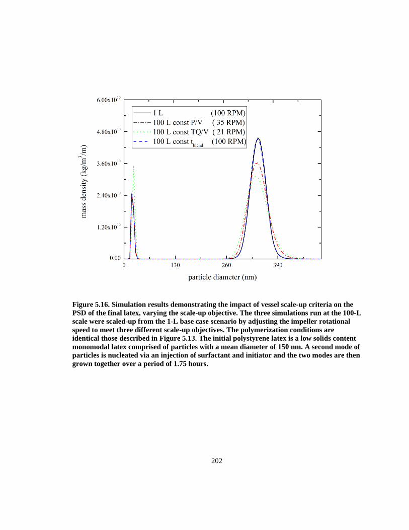
202
Figure 5.16. Simulation results demonstrating the impact of vessel scale-up criteria on the
PSD of the final latex, varying the scale-up objective. The three simulations run at the 100-L
scale were scaled-up from the 1-L base case scenario by adjusting the impeller rotational
speed to meet three different scale-up objectives. The polymerization conditions are
identical those described in Figure 5.13. The initial polystyrene latex is a low solids content
monomodal latex comprised of particles with a mean diameter of 150 nm. A second mode of
particles is nucleated via an injection of surfactant and initiator and the two modes are then
grown together over a period of 1.75 hours.
203
Figure 5.17. Simulation results demonstrating the impact of vessel scale-up criteria on the
PSD of the final latex. The reactor is scale-up from 1 L to 10 m3 using the constant torque-
per-unit-volume (TQ/V) approach. The polymerization conditions are identical those
described in Figure 5.13. The initial polystyrene latex is a low solids content monomodal
latex comprised of particles with a mean diameter of 150 nm. A second mode of particles is
nucleated via an injection of surfactant and initiator and the two modes are then grown
together over a period of 1.75 hours.
The packing model developed by Pishvaei et al.
5 may be used to compute estimates of the
packing parameters and, therefore, predict a priori latex rheological properties using the PSD
data. In Figure 5.18a, the relationship between reactor scale and the theoretical zero-shear
maximum packing fraction of the product latex is shown. The zero-shear maximum packing
fractions can be entered into the Kreiger-Dougherty equation to produce estimates of the latex
viscosities at zero shear, which is shown in Figure 5.18b. The estimates of maximum packing
204
fraction appear to be very high, although this can be partially-explained by the very wide PSDs.
At the 10-m3 scale, the final particle size distribution is especially wide if the process is scaled-up
with a constant TQ/V, leading to a product with a lower zero-shear viscosity compared to the
product obtained from the same process when it is scaled-up with a constant P/V. Finally it is
noted that the viscosity is lowest (which is desirable) at the 1 L scale; this is due to the fact that
the PSD at the 1 L scale has diameter and mass ratios that are closer the optimum from a
perspective of maximizing particle packing.
The above simulation work establishes the combined CFD/PBM framework is a very useful tool
for modeling the scale-up of emulsion polymerization processes. Such results would otherwise be
unavailable for consideration during the scale-up process. The objective of this work was to
establish the approach, build the required interface and run a set of preliminary calculations.
Future work will extend the functionality of the framework. For example, the assumption of
isothermal operation should be relaxed. At large reactor scales, the model predicts an
accumulation of reactants in the vicinity of the feed zone. The enhanced rate of particle
nucleation and coagulation observed in this zone may lead to the formation of a local hotspot due
to two mechanisms: (i) an increase in the concentration of small particles increases the local rate
of polymerization and (ii) excessive particle coagulation could lead to an increase in local fluid
viscosity, potentially reducing rate of flow and, hence, energy exchanged between the zone and
its surroundings. Any changes in reactor temperature would be accompanied by changes in fluid
viscosity, so the model framework is especially well-suited for modeling non-isothermal
operation.
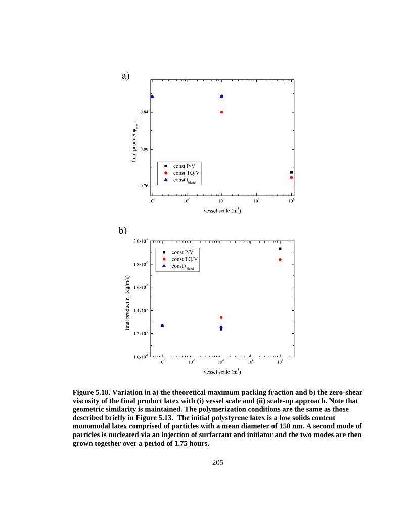
205
Figure 5.18. Variation in a) the theoretical maximum packing fraction and b) the zero-shear
viscosity of the final product latex with (i) vessel scale and (ii) scale-up approach. Note that
geometric similarity is maintained. The polymerization conditions are the same as those
described briefly in Figure 5.13. The initial polystyrene latex is a low solids content
monomodal latex comprised of particles with a mean diameter of 150 nm. A second mode of
particles is nucleated via an injection of surfactant and initiator and the two modes are then
grown together over a period of 1.75 hours.
206
5.5 Conclusion
The hybrid network-of-zones population balance / CFD computational framework is capable of
providing unique insight into the scale-up of emulsion polymerization processes, while still being
economical enough to apply in an industrial environment. Tracer dispersion simulations indicate
that, under realistic conditions, the amount of time required to blend reactants that are introduced
under semi-batch feed will increase with reactor scale. The blending data can be used to divide
the reactor into a network-of-zones to directly model and predict the impact of a longer reactant
blend time on the time-evolution of latex PSD during a semi-batch styrene EP. The framework
predicts that limitations in reactant blending will affect the PSD and rheological properties of the
final product. When blending is particularly poor, latex destabilization and scrap formation may
become an issue. From an industrial point of view, the framework holds promise as a tool for
developing scale-up rules and strategies that minimize differences in PSD upon scale-up.
Application of the framework is currently limited to processes where the mixing restrictions are
critical over a short time frame only, such that the liquid level can be assumed to be constant.
Future development will focus on improving the framework to accommodate large changes in the
liquid level and relaxing the assumption of isothermal operation, so that the framework will be
applicable to a wider range of emulsion polymerization processes.
207
Chapter 6
Concluding Remarks
6.1 Summary of Results
The emergence of robust and affordable computational fluid dynamics (CFD) software has
revolutionized process scale-up, as process engineers no longer have to rely solely on heuristics
(and experience) to ensure that primary mixing objectives are met at each successive process
scale. The production of polymer latexes via emulsion polymerization is, however, a highly
complex process with multiple mixing-objectives. For such a process, the development of a
process model that accounts for non-homogeneity in the flow field will reduce the time and
money required for scale up, production and, finally, commercialization. Due to the
computational resources required, it is currently it is unfeasible to program a population balance
equation-based process model directly into the CFD simulation code, but hybrid modeling, where
the process model is solved on a much coarser mesh, has emerged as a viable approach. It had
been demonstrated that a combined CFD-population balance modeling (PBM) approach could be
used to study the effect of reactor configuration on the mechanically-induced coagulation of
polymer lattices, but the process model was heavily-simplified. A survey of the literature
suggested that the development of a combined CFD-PBM modeling framework that was designed
to investigate process scale-up was the next logical step.
As explained in Chapter 3, recent advances in our understanding of colloidal interactions between
polymer latex particles has resulted in the emergence of a DLVO-based coagulation kernels that
is capable of reproducing theoretical results, hitherto only available through a time-consuming
208
solution to the Smoluchowksi convection-diffusion aggregation equation in two dimensions over
a full range of shearing conditions. Researchers are in disagreement as to whether shear-induced
coagulation is relevant in emulsion polymerization at the laboratory scale, but its effect is known
to be an issue at the industrial scale and is thought to be caused by turbulence. Our preliminary
CFD simulations suggest that while the amount of turbulence in the flow increases with reactor
scale, the maximum rate of shear due to turbulence inside the reactor may not. However, further
simulation work with more refined computational meshes will be necessary in order to confirm
that the characteristics of the trailing vortices, where the highest shear rates are encountered, are
being captured properly. At both the laboratory and commercial scales, the maximum shear rate is
large enough to influence the overall rate of particle aggregation, but not under all conditions.
Larger particles and particles with more diffuse stabilization layers will be more sensitive to
mechanical coagulation and may be affected within a larger region of the vessel. A comparison of
a state-of-the-art coagulation model with a less computationally-intensive coagulation model
suggests that the latter model will over-predict the influence of mechanical shear on the rate of
particle coagulation. The discrepancy can be reduced (but not eliminated) by replacing the
standard particle Peclet number with a Peclet number modified to account for interparticle
interactions. If the dispersed media has a high ionic strength, as would be encountered when a
latex is purposefully-coagulated via the addition of an electrolyte, the effects of mechanical
agitation will be largely diminished.
In Chapter 4, using a previously-published emulsion polymerization process model, a hybrid
CFD-PBM framework was constructed to examine the effects of process scale-up on the
coagulation of high solids content latexes. The study was restricted to reactors operating under
209
the laminar and early transition regimes. Using specialized CFD simulation code that had been
developed and experimentally-validated for non-Newtonian fluids, it was shown that the
framework could be used to investigate the impact of reactor scale-up on the development of the
latex particle size distribution over the course of a reaction.
As described in Chapter 4, the first version of the framework was restrictive. The CFD simulation
code, POLY3D, was not adapted to study turbulent flow and the automatic zoning algorithm was
simplistic in nature. To assuage some of the framework‟s limitations, a recently published
automatic layer-by-layer zoning algorithm was implemented within with Fluent®, a commercial
CFD package designed to model both laminar and turbulent flow. By manipulating the transient
species-tracking simulation data, it is possible to compute the amount of time it takes the
reactants, which are fed in near the impeller tip, to reach every region of the reactor. The
approach of using transient species-tracking data to compartmentalize the reactor has not been
previously-published. The network of zones generated using this technique allows us to directly
include the influence of inhomogeneous mixing inside the process model.
Combined with an up-to-date styrene emulsion polymerization population balance model, it was
demonstrated in Chapter 5 that the framework is well-suited to investigating the scale-up of
styrene emulsion polymerization, where the target PSD was bimodal. Simulation results indicated
that the slow dispersal of surfactant and initiator, a problem that emerges at the pilot- and
commercial- scales, results in much higher rates of particle nucleation and particle coagulation in
and near the feed zone, resulting in the final product having a different particle size distribution.
Three approaches to scale-up were examined (geometric similarity was assumed) and it was
found that the final PSD was reproduced only when the reactor was scaled up based on the
210
objective of maintaining a constant blend time. As the reactor‟s blend time increases, the
reproduction of the laboratory-scale PSD worsened, regardless of the scale. This shows that very
relevant results can be determined using this framework that, otherwise, are unavailable in reactor
design.
6.2 Recommendations
During this feasibility study, focus was concentrated on the approach, building the interface and
preliminary calculations. In order to examine a wider range of emulsion polymerization
processes, the framework, as demonstrated in Chapter 5, should be extended account for a
variable liquid level. Without a variable liquid-level functionality programmed into the process
model, the framework is restricted to modeling emulsion polymerization reactions where the
mixing-critical step of the reaction occurs over a short time period.
It is recommended that the framework be extended by incorporating a set of energy balance
equations into the process model, along with means of estimating the heat transfer coefficient at
the reactor wall using CFD simulation. The assumption of isothermal operation may be invalid,
particularly in reactors where mixing is poor and larger reactor scales where the volume-
normalized surface available for heat transfer is reduced. By incorporating a set of energy balance
equations into the process model, the framework may be a useful tool for studying the emergence
of hotspots in the reactor.
211
In order to model a wider range of semi-batch processes, the multizonal process model must be
designed to capture the effect of mixing restrictions which play out over a larger timescale where
liquid level will increase. Tracer dispersal simulations indicate that the pattern of tracer dispersion
varies near the surface of the latex (i.e. momentum near the free surface is affected by the surface
boundary conditions), but does not vary much below the surface. Using experimental flow-
visualization and quantification techniques (e.g. particle imaging velocimetry), it may be possible
to develop a correction factor such that CFD simulation results based on a full tank can be used to
generate the process model grid and the interzonal flow rates could be updated each time the
liquid level changes by a threshold value.
While the latest coagulation models are able to account for both shear-related and DLVO-related
interaction forces, the complex procedure required to compute the fitting parameters at every time
step is a problem. There are two solution approaches that may be investigated: (i) the generation
of a large, multi-dimensional data set that tabulates the parameter values for a given set of particle
radii, particle surface potentials and ionic strength; (ii) the creation of a simplified procedure for
computing the parameters and prefactors that does not require root-finding for a function
containing an integral term. The former approach (data tables) is used in industrial processes, but
the latter approach may be more practical for our purposes. Due to the transient nature of
turbulence, the use of a more accurate transient turbulence model (i.e. a Large Eddy-type
turbulence model) may offer improved insight regarding the influence of reactor scale on the
spatial distribution of the particle Peclet number. The coagulation model could be further
augmented by including (separately) the contributions of surface coagulation, which is brought
about by foaming at the liquid-air interface at the surface. Further developments in state-of-the-art
212
coagulation modeling combined with a more-advanced CFD simulation framework may justify
the use of the hybrid model framework to study the impact of vessel scale-up on the
mechanically-induced coagulation of polymer latexes.
Finally, it is noted that while the models used to construct the framework were chosen because
they had been modeled experimentally, there is still a need to validate the predictive capabilities
of the hybrid CFD/PBM modeling approach with experimentally obtained data. The best
opportunity to validate the framework at large reactor scales lies with industry, due to the large
amount of confidential process plant data already available. Within the academic research
community, pilot-scale experimentation may be possible, and the use of scale-down models as an
alternative validation technique also warrants investigation.
213
References
1. de la Cal, J. C.; Leiza, J. R.; Asua, J. M.; Butte, A. Emulsion Polymerization. In Handbook of
Polymer Reaction Engineering; Meyer, T., Keurentjes, J., Eds.; Wiley-VCH Verlag GmbH &
Co.: Weinheim, Germany, 2005; pp 249-322.
2. Blackley, D. C. Polymer latices : science and technology; Chapman & Hall: London; New
York, 1997; .
3. Smith, W. E.; Ewart, R. H. J. Chem. Phys. 1948, 6, 592-599.
4. Gilbert, R. G. Emulsion Polymerization: A Mechanistic Approach; Academic Press Limited:
San Diego, USA, 1995; .
5. Pishvaei, M.; Graillat, C.; McKenna, T. F.; Cassagnau, P. J. Rheol. 2007, 1, 51-69.
6. Ouzineb, K.; Graillat, C.; McKenna, T. F. J. Appl. Polym. Sci. 2005, 3, 745-752.
7. Vale, H. Population Balance Modeling of Emulsion Polymerization Reactors: Applications to
Vinyl Chloride Polymerization, University Claude Bernard Lyon 1, Lyon, France, 2007.
8. Vale, H. M.; McKenna, T. F. Prog. Polym. Sci. 2005, 10, 1019-1048.
9. Boutti, S.; Graillat, C.; McKenna, T. F. Polymer 2005, 4, 1223-1234.
10. Oldshue, J. Y. Fluid Mixing Technology; McGraw-Hill: New York, NY, 1983; , pp 574.
11. Versteeg, H. K.; Malalasekera, W. An introduction to computational fluid dynamics: The
finite volume method; Pearson - Prentice Hall: Harlow, England, 2007; , pp 503.
12. Wang, H.; Chen, H.; Periaux, J. Int. J. Numer. Methods Fluids 2010, 1, 98-118.
13. Marshall, E. M.; Bakker, A. Computational fluid mixing. In Handbook of Industrial Mixing;
Paul, E. L., Atiemo-Obeng, V. A. and Kresta, S. M., Eds.; Wiley-Interscience: Hoboken, NJ,
2004; pp 257-343.
214
14. Foucault, S.; Ascanio, G.; Tanguy, P. A. Ind. Eng. Chem. Res. 2006, 1, 352-359.
15. Alexopoulos, A. H.; Kiparissides, C. Prediction of particle size distribution in non-
homogeneous particulate systems: Two compartment model of an emulsion polymerization
reactor. In International symposium on polymers in dispersed media. McKenna, T. F., Bourgeat-
Lami, E. and Elaissari, A., Eds.; Lyon, 2004; pp 34-36.
16. Elgebrandt, R. C.; Romagnoli, J. A.; Fletcher, D. F.; Gomes, V. G.; Gilbert, R. G. Chem. Eng.
Sci. 2005, 7, 2005-2015.
17. Elgebrandt, R. C.; Fletcher, D. F.; Gomes, V. G.; Romagnoli, J. A. A framework for modeling
particle size effects in emulsion polymerization systems using computational fluid mechanics
linked to a detailed population balance model. In 16th European Symposium on Computer Aided
Process Engineering and 9th International Symposium on Process Systems Engineering;
Marquardt, W., Pantelides, C. C., Eds.; Elsevier B.V.: 2006; pp 551-556.
18. Harkins, W. D. J. Am. Chem. Soc. 1947, 6, 1428-1444.
19. Chern, C. S. Prog. Polym. Sci. 2006, 443-486.
20. Kohut-Svelko, N.; Pirri, R.; Asua, J. M.; Leiza, J. R. Journal of Polymer Science Part A:
Polymer Chemistry 2009, 11, 2917-2927.
21. Thickett, S. C.; Gilbert, R. G. Polymer 2007, 24, 6965-6991.
22. Chern, C.; Lin, C. Polymer 1999, 1, 139-147.
23. Zubitur, M.; Mendoza, J.; Cal, J. C. d. l.; Asua, J. M. Macromol. Symp. 2000, 1, 13-22.
24. Achilias, D. S.; Kiparissides, C. Macromolecules 1992, 14, 3739-3750.
25. Zubitur, M.; Asua, J. M. Polymer, 2001, 14, 5979-5985.
26. Boutti, S.; Graillat, C.; McKenna, T. F. Macromol. Symp. 2004, 1, 383-398.
215
27. Ai, Z.; Zhou, Q.; Xie, C.; Zhang, H. J. Appl. Polym. Sci. 2007, 3, 1815-1825.
28. Greenwood, R.; Luckham, P. F.; Gregory, T. J. Col. Int. Sci. 1997, 1, 11-21.
29. Smith, W. E.; Zukoski, C. F. J. Rheol. 2004, 6, 1375-1388.
30. Guyot, A.; Chu, F.; Schneider, M.; Graillat, C.; McKenna, T. F. Prog. Polym. Sci. 2002, 8,
1573-1615.
31. Schneider, M.; Claverie, J.; Graillat, C.; McKenna, T. F. J. Appl. Polym. Sci. 2002, 10, 1878-
1896.
32. Greenwood, R.; Luckham, P. F.; Gregory, T. Colloid Surf. A 1998, 1-3, 139-147.
33. Schneider, M.; Graillat, C.; Guyot, A.; Betrémieux, I.; McKenna, T. F. J. Appl. Polym. Sci.
2002, 10, 1935-1948.
34. Schneider, M.; Graillat, C.; Guyot, A.; McKenna, T. F. J. Appl. Polym. Sci. 2002, 10, 1916-
1934.
35. Schneider, M.; Graillat, C.; Guyot, A.; McKenna, T. F. J. Appl. Polym. Sci. 2002, 10, 1897-
1915.
36. Boutti, S.; Graillat, C.; McKenna, T. F. Polymer 2005, 4, 1189-1210.
37. Boutti, S.; Graillat, C.; McKenna, T. F. Polymer 2005, 4, 1211-1222.
38. Mayo, F. R.; Lewis, F. M. J. Am. Chem. Soc. 1944, 9, 1594-1601.
39. Heuts, J. P. A.; Russell, G. T.; Smith, G. B.; van Herk, A. M. Macromol. Symp. 2007, 1, 12-
22.
40. Buback, M.; Egorov, M.; Gilbert, R. G.; Kaminsky, V.; Olaj, O. F.; Russell, G. T.; Vana, P.;
Zifferer, G. Macromol. Chem. Phys. 2002, 18, 2570-2582.
216
41. Kemmere, M. F.; Meuldijk, J.; Drinkenburg, A. A. H.; German, A. L. J. Appl. Polym. Sci.
1998, 12, 2409-2421.
42. Melis, S.; Kemmere, M.; Meuldijk, J.; Storti, G.; Morbidelli, M. Chem. Eng. Sci. 2000, 16,
3101-3111.
43. Forcolin, S.; Marconi, A. M.; Ghielmi, A.; Butte, A.; Storti, G.; Morbidelli, M. Plast. Rubber
Compos. 1999, 3, 109-115.
44. Melis, S.; Verduyn, M.; Storti, G.; Morbidelli, M.; Baldyga, J. AICHE J. 1999, 7, 1383-1393.
45. Lowry, V.; El-Aasser, M. S.; Vanderhoff, J. W.; Klein, A. J. Appl. Polym. Sci. 1984, 12,
3925-3935.
46. Lowry, V.; El-Aasser, M. S.; Vanderhoff, J. W.; Klein, A.; Silebi, C. A. J. Col. Int. Sci. 1986,
2, 521-529.
47. Lattuada, M.; Morbidelli, M. J. Colloid Interface Sci. 2011, 1, 42.
48. Heller, W.; Peters, J. J. Colloid Interface Sci. 1970, 4, 592-605.
49. Peters, J.; Heller, W. J. Colloid Interface Sci. 1970, 4, 578-585.
50. Heller, W.; De Lauder, W. B. J. Colloid Interface Sci. 1971, 1, 60-65.
51. Heller, W.; Peters, J. J. Colloid Interface Sci. 1971, 2, 300-307.
52. Delauder, W. B.; Heller, W. J. Colloid Interface Sci. 1971, 2, 308-313.
53. Ottewill, R. H. Stability of polymer colloids. In Polymeric Dispersions: Principles and
Applications; Asua, J. M., Ed.; Kluwer Academic Publishers: Boston, 1997; pp 31-48.
54. Hoffman, R. L. J. Rheol. 1998, 1, 111-123.
55. Einstein, A. Annalen der Physik 1906, 2, 289-306.
217
56. Einstein, A. Annalen der Physik 1911, 3, 590-590.
57. Sudduth, R. D. J. Appl. Polym. Sci. 1993, 1, 25-36.
58. Krieger, I. M.; Dougherty, T. J. J. Rheol. 1959, 1, 137-152.
59. Mooney, M. J. Col. Sci. 1951, 2, 162-170.
60. Sudduth, R. D. J. Appl. Polym. Sci. 1993, 1, 123-147.
61. Ouchiyama, N.; Tanaka, T. Ind. Eng. Chem. Fundam. 1980, 338-340.
62. Ouchiyama, N.; Tanaka, T. Ind. Eng. Chem. Fundam. 1981, 66-71.
63. Ouchiyama, N.; Tanaka, T. Ind. Eng. Chem. Fundam. 1984, 490-493.
64. Ouchiyama, N.; Tanaka, T. Ind. Eng. Chem. Fundam. 1986, 1, 125-129.
65. Pishvaei, M.; Cassagnau, P.; McKenna, T. F. Macromol. Symp. 2006, 1, 63-71.
66. Sukumar, N. Int J Numer Methods Eng 2003, 1, 1-34.
67. Bharat K., S. Applied Numerical Mathematics 2000, 4, 361-369.
68. Bathe, K. J. Finite Element Procedures; 1996; .
69. Danckwerts, P. Applied Scientific Research 1952, 4, 279-296.
70. Kresta, S. M.; Brodkey, R. S. 2004, 19-87.
71. Mohr, W. D.; Saxton, R. L.; Jepson, C. H. Industrial & Engineering Chemistry 1957, 11,
1855-1856.
72. Aref, H. J. Fluid Mech. 1984, 1-21.
218
73. Szalai, E. S.; Alvarez, M. M.; Muzzio, F. J. 2004, 89-143.
74. Aubin, J.; Fletcher, D. F.; Xuereb, C. Exp. Therm. Fluid Sci. 2004, 5, 431-445.
75. Brown, D. A. R.; Jones, P. N.; Middleton, J. C.; Papadopoulos, G.; Arik, E. B. 2004, 145-256.
76. Kukukova, A.; Aubin, J.; Kresta, S. M. Chem. Eng. Res. Design 2009, 4, 633-647.
77. Joshi, J. B.; Nere, N. K.; Rane, C. V.; Murthy, B. N.; Mathpati, C. S.; Patwardhan, A. W.;
Ranade, V. V. The Canadian Journal of Chemical Engineering 2011, 4, 754-816.
78. Bezzo, F.; Macchietto, S.; Pantelides, C. C. Comp. Chem. Eng. 2004, 4, 501-511.
79. Bezzo, F.; Macchietto, S.; Pantelides, C. C. AICHE J. 2003, 8, 2133-2148.
80. Bezzo, F.; Macchietto, S. Comp. Chem. Eng. 2004, 4, 513-525.
81. Bezzo, F.; Macchietto, S.; Pantelides, C. C. AIChE J. 2005, 4, 1169-1177.
82. Gresch, M.; Brügger, R.; Meyer, A.; Gujer, W. Environ. Sci. Technol. 2009, 7, 2381-2387.
83. Alexopoulos, A. H.; Maggioris, D.; Kiparissides, C. Chem. Eng. Sci. 2002, 10, 1735-1752.
84. Schäfer, M.; Yianneskis, M.; Wächter, P.; Durst, F. AICHE J. 1998, 6, 1233-1246.
85. Jung, S. M.; Gomes, V. G. Chemical Engineering Science 2011, 18, 4251.
86. Seppälä, M. Automatic zoning for combined CFD and multiblock modelling, Helsinki
University of Technology, 2008.
87. Hemrajani, R. R.; Tatterson, G. B. Mechanically stirred vessels. In Handbook of Industrial
Mixing; Paul, E. L., Atiemo-Obeng, V. A. and Kresta, S. M., Eds.; Wiley-Interscience: Hoboken,
NJ, 2004; pp 345-390.
219
88. Pohn, J.; Heniche, M.; Fradette, L.; Cunningham, M.; McKenna, T. Chem. Eng. Technol.
2010, 11, 1917-1930.
89. Ramkrishna, D. Population Balances: Theory and Applications to Particulate Systems in
Engineering; Academic Press: London, UK, 2000; , pp 355.
90. Fuchs, N. Zeitschrift für Physik A Hadrons and Nuclei 1934, 11, 736-743.
91. Smoluchowski, M. v. Z. Phys. Chem. 2010, 129.
92. Verwey, E. J. W. The Journal of Physical and Colloid Chemistry 1947, 3, 631-636.
93. Hong, J. Effects of Agitation in Emulsion Polymerization - Kinetic and Mechanistic Study of
Coagulum, 2008.
94. M.V., S. Zeitschrift fur Physik 1916, 557-585.
95. Batchelor, G. K.; Green, J. T. J. Fluid Mech. 1972, 02, 375.
96. Behrens, S. H.; Christl, D. I.; Emmerzael, R.; Schurtenberger, P.; Borkovec, M. Langmuir
2000, 6, 2566-2575.
97. Honig, E. P.; Roebersen, G. J.; Wiersema, P. H. J. Colloid Interface Sci. 1971, 1, 97.
98. Jia, Z.; Gauer, C.; Wu, H.; Morbidelli, M.; Chittofrati, A.; Apostolo, M. J. Colloid Interface
Sci. 2006, 1, 187-202.
99. Coen, E. M.; Gilbert, R. G.; Morrison, B. R.; Leube, H.; Peach, S. Polymer, 1998, 26, 7099-
7112.
100. Fortuny, M.; Graillat, C.; McKenna, T. F. Ind Eng Chem Res 2004, 23, 7210-7219.
101. Hogg, R.; Healy, T. W.; Fuerstenau, D. W. Trans. Faraday Soc. 1966.
102. Liu, B.; Hsu, J. J. Chem. Phys. 2009, 4, 044106.
220
103. Zeaiter, J.; A. Romagnoli, J.; W. Barton, G.; G. Gomes, V.; S. Hawkett, B.; G. Gilbert, R.
Chem. Eng. Sci. 2002, 15, 2955-2969.
104. Immanuel, C. D.; Cordeiro, C. F.; Sundaram, S. S.; Meadows, E. S.; Crowley, T. J.; III, F. J.
D. Comput. Chem. Eng. 2002, 7-8, 1133.
105. Fluent 2006.
106. Montante, G.; Mostek, M.; Jahoda, M.; Magelli, F. Chem. Eng. Sci. 2005, 8-9, 2427-2437.
107. Deglon, D. A.; Meyer, C. J. Minerals Eng 2006, 10, 1059-1068.
108. Gori, F.; Boghi, A. Int. Commun. Heat Mass Transfer 2011, 6, 696.
109. Rudman, M.; Blackburn, H. M. Appl. Math. Modelling 2006, 11, 1229-1248.
110. Doraiswamy, D.; Grenville, R. K.; Etchells, A. W. Ind Eng Chem Res 1994, 10, 2253-2258.
111. Wu, B.; Chen, S. Biotechnol. Bioeng. 2008, 3, 700-711.
112. Nouri, J. M.; Hockey, R. M. J. Chem. Eng. Jap. 1998, 5, 848-852.
113. Pishvaei, M.; Graillat, C.; McKenna, T. F.; Cassagnau, P. Polymer 2005, 4, 1235-1244.
114. Kostansek, E. Journal of Coatings Technology and Research 2004, 1, 41-44.
115. Tatterson, G. B. Fluid mixing and gas dispersion in agitated tanks; McGraw-Hill: New
York, NY, 1991; , pp 548.
116. Kresta, S. M.; Krebs, R.; Martin, T. Chem. Eng. Technol. 2004, 3, 208-214.
117. Mavros, P. Chem. Eng. Res. Des. 2001, 2, 113-127.
118. Patel, H.; Ein-Mozaffari, F.; Dhib, R. Comput. Chem. Eng. 2010, 4, 421-429.
221
119. Maggioris, D.; Goulas, A.; Alexopoulos, A. H.; Chatzi, E. G.; Kiparissides, C. Chem. Eng.
Sci. 1998, S315-S322.
120. Bezzo, F.; Macchietto, S.; Pantelides, C. C. Comp. Chem. Eng. 2000, 2-7, 653-658.
121. Kumar, S.; Ramkrishna, D. Chemical Engineering Science 1996, 8, 1311-1332.
122. Butté, A.; Storti, G.; Morbidelli, M. Macromolecular Theory and Simulations 2002, 1, 37-
52.
123. McGown, D. N. L.; Parfitt, G. D. J. Phys. Chem. 1967, 2, 449-450.
124. Eastman, J. Colloid Stability. In Colloid Science; Cosgrove, T., Ed.; 2009; pp 36-49.
125. Coesnon, B.; Heniche, M.; Devals, C.; Bertrand, F.; Tanguy, P. A. Int. J. Numer. Methods
Fluids 2008, 4, 427-449.
126. Radhakrishnan, K.; Hindmarsh, A. C. 1993.
127. Kemmere, M. F. Batch emulsion polymerization: A chemical engineering approach,
Eindhoven University of Technology, Eindhoven, 1999.
128. Vale, H. M.; McKenna, T. F. Ind Eng Chem Res 2007, 2, 643-654.
129. Meadows, E. S.; Crowley, T. J.; Immanuel, C. D.; Doyle, F. J. Ind Eng Chem Res 2003, 3,
555-567.
130. Guha, D.; Dudukovic, M. P.; Ramachandran, P. A.; Mehta, S.; Alvare, J. AICHE J. 2006, 5,
1836-1846.
131. Hansen, F. K.; Ugelstad, J. J. Polym. Sci. Polym. Chem. Ed. 1978, 8, 1953-1979.
132. Maxwell, I. A.; Morrison, B. R.; Napper, D. H.; Gilbert, R. G. Macromolecules 1991, 7,
1629-1640.
222
133. Russell, G. T.; Napper, D. H.; Gilbert, R. G. Macromolecules 1988, 7, 2141-2148.
134. Taylor, D. R.; van Berkel, K. Y.; Alghamdi, M. M.; Russell, G. T. Macromolecular
Chemistry and Physics 2010, 5, 563-579.
135. Marten, F. L.; Hamielec, A. E. J Appl Polym Sci 1982, 2, 489-505.
136. Green, D. W.; Perry, R. H. 2008.
137. Orwoll, R. 2007, 93-101.
138. Giannetti, E. AICHE J. 1993, 7, 1210-1227.
139. Piirma, I.; Chen, S. J. Colloid Interface Sci. 1980, 1, 90-102.
140. Mukerjee, P.; Mysels, K. J. NSRDS-NBS 1971, 1-222.
141. Bales, B. L.; Messina, L.; Vidal, A.; Peric, M.; Nascimento, O. R. The Journal of Physical
Chemistry B 1998, 50, 10347-10358.
142. Vanzo, E.; Marchessault, R. H.; Stannett, V. J. Colloid Sci. 1965, 1, 62.
143. Coen, E. M.; Peach, S.; Morrison, B. R.; Gilbert, R. G. Polymer 2004, 3595-3608.
144. O'Toole, J. T. J. Appl. Polym. Sci. 1963, 4, 1291-1297.
145. Jiang, G.; Shu, C. Journal of Computational Physics 1996, 1, 202.
146. Wang, R.; Feng, H.; Spiteri, R. J. Applied Mathematics and Computation 2008, 1, 433.