Scalable algorithms for Jitter minimized scheduling in

reconfigurable CoEDivya Chitimalla

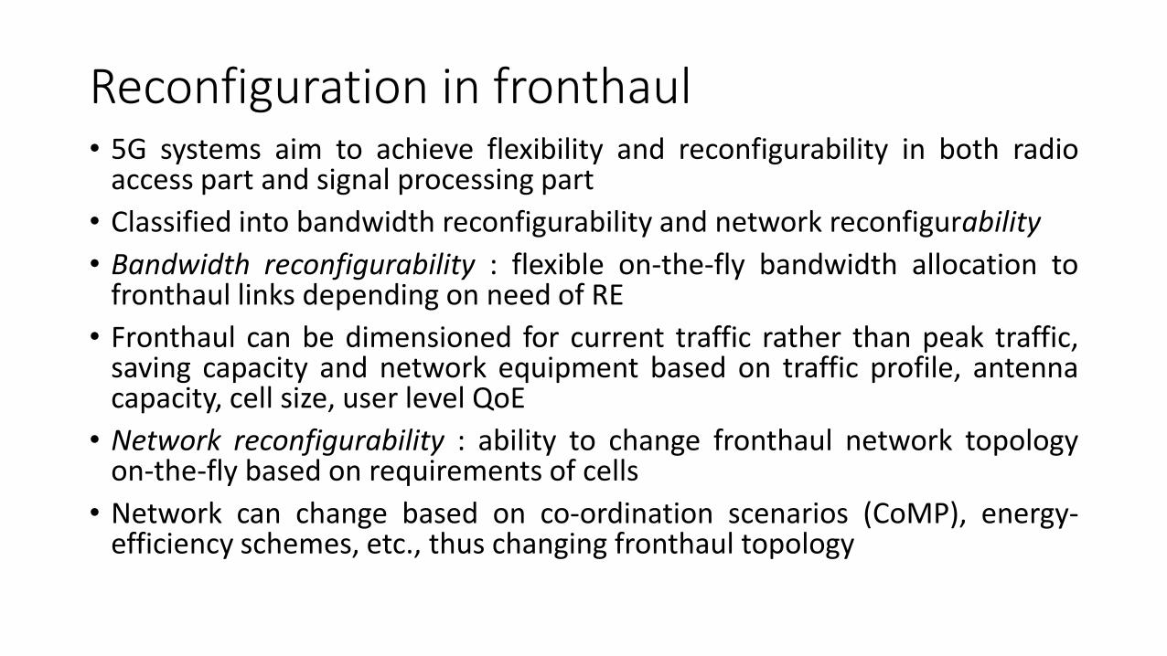
Reconfiguration in fronthaul• 5G systems aim to achieve flexibility and reconfigurability in both radio

access part and signal processing part

• Classified into bandwidth reconfigurability and network reconfigurability

• Bandwidth reconfigurability : flexible on-the-fly bandwidth allocation tofronthaul links depending on need of RE

• Fronthaul can be dimensioned for current traffic rather than peak traffic,saving capacity and network equipment based on traffic profile, antennacapacity, cell size, user level QoE

• Network reconfigurability : ability to change fronthaul network topologyon-the-fly based on requirements of cells

• Network can change based on co-ordination scenarios (CoMP), energy-efficiency schemes, etc., thus changing fronthaul topology

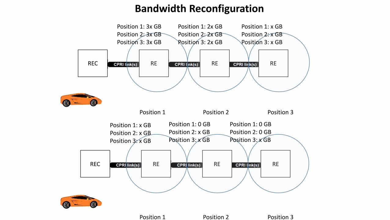
REC RE RE RE

REC RE RE RE

Position 1: 3x GBPosition 2: 3x GBPosition 3: 3x GB

Position 1: 2x GBPosition 2: 2x GBPosition 3: 2x GB

Position 1: x GBPosition 2: x GBPosition 3: x GB

Position 1 Position 2 Position 3

Position 1: x GBPosition 2: x GBPosition 3: x GB

Position 1: 0 GBPosition 2: x GBPosition 3: x GB

Position 1: 0 GBPosition 2: 0 GBPosition 3: x GB

Position 1 Position 2 Position 3

Bandwidth Reconfiguration

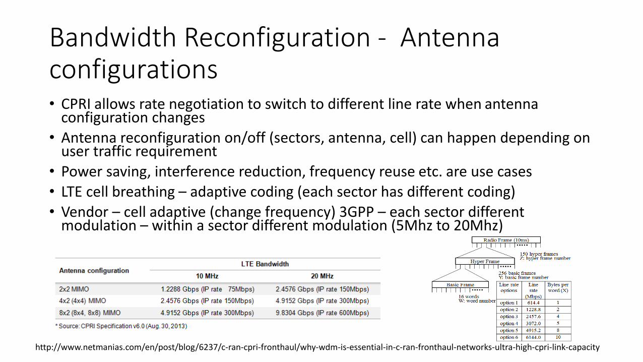
Bandwidth Reconfiguration - Antenna configurations• CPRI allows rate negotiation to switch to different line rate when antenna

configuration changes

• Antenna reconfiguration on/off (sectors, antenna, cell) can happen depending on user traffic requirement

• Power saving, interference reduction, frequency reuse etc. are use cases

• LTE cell breathing – adaptive coding (each sector has different coding)

• Vendor – cell adaptive (change frequency) 3GPP – each sector different modulation – within a sector different modulation (5Mhz to 20Mhz)

http://www.netmanias.com/en/post/blog/6237/c-ran-cpri-fronthaul/why-wdm-is-essential-in-c-ran-fronthaul-networks-ultra-high-cpri-link-capacity

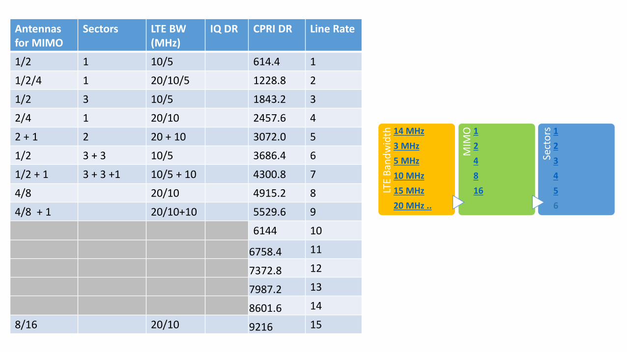
Antennasfor MIMO

Sectors LTE BW (MHz)

IQ DR CPRI DR Line Rate

1/2 1 10/5 614.4 1

1/2/4 1 20/10/5 1228.8 2

1/2 3 10/5 1843.2 3

2/4 1 20/10 2457.6 4

2 + 1 2 20 + 10 3072.0 5

1/2 3 + 3 10/5 3686.4 6

1/2 + 1 3 + 3 +1 10/5 + 10 4300.8 7

4/8 20/10 4915.2 8

4/8 + 1 20/10+10 5529.6 9

6144 10

6758.4 11

7372.8 12

7987.2 13

8601.6 14

8/16 20/10 9216 15

LTE

Ban

dw

idth 14 MHz

3 MHz

5 MHz

10 MHz

15 MHz

20 MHz ..

MIM

O 1

2

4

8

16

Sect

ors 1

2

3

4

5

6

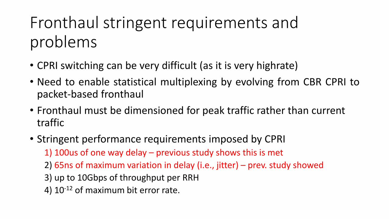
Fronthaul stringent requirements and problems• CPRI switching can be very difficult (as it is very highrate)

• Need to enable statistical multiplexing by evolving from CBR CPRI topacket-based fronthaul

• Fronthaul must be dimensioned for peak traffic rather than current traffic

• Stringent performance requirements imposed by CPRI1) 100us of one way delay – previous study shows this is met

2) 65ns of maximum variation in delay (i.e., jitter) – prev. study showed

3) up to 10Gbps of throughput per RRH

4) 10-12 of maximum bit error rate.

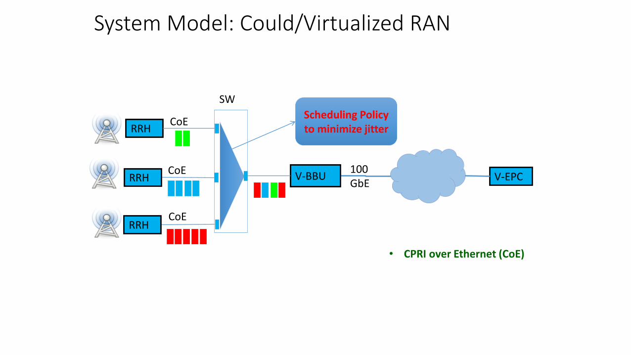
• CPRI over Ethernet (CoE)

System Model: Could/Virtualized RAN

RRH

V-EPC100GbE

V-BBURRH

RRH

CoE

CoE

CoE

SW

Scheduling Policy to minimize jitter

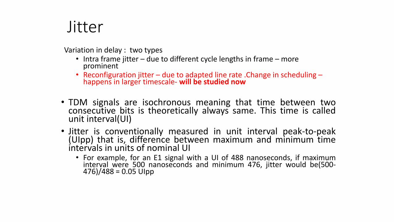
JitterVariation in delay : two types

• Intra frame jitter – due to different cycle lengths in frame – more prominent

• Reconfiguration jitter – due to adapted line rate .Change in scheduling –happens in larger timescale- will be studied now

• TDM signals are isochronous meaning that time between twoconsecutive bits is theoretically always same. This time is calledunit interval(UI)

• Jitter is conventionally measured in unit interval peak-to-peak(UIpp) that is, difference between maximum and minimum timeintervals in units of nominal UI• For example, for an E1 signal with a UI of 488 nanoseconds, if maximum

interval were 500 nanoseconds and minimum 476, jitter would be(500-476)/488 = 0.05 UIpp

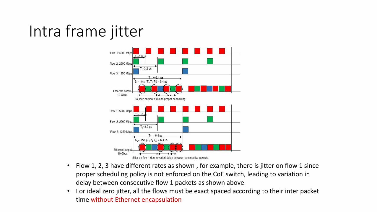
Intra frame jitter

• Flow 1, 2, 3 have different rates as shown , for example, there is jitter on flow 1 since proper scheduling policy is not enforced on the CoE switch, leading to variation in delay between consecutive flow 1 packets as shown above

• For ideal zero jitter, all the flows must be exact spaced according to their inter packet time without Ethernet encapsulation

(a)

(b)Figure 4: (a) An example that shows jitter on flow 1; (b) An

example that shows how proper scheduling can eliminate jitter.

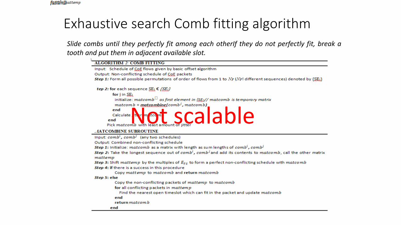
Exhaustive search Comb fitting algorithmSlide combs until they perfectly fit among each otherIf they do not perfectly fit, break atooth and put them in adjacent available slot.

Not scalable

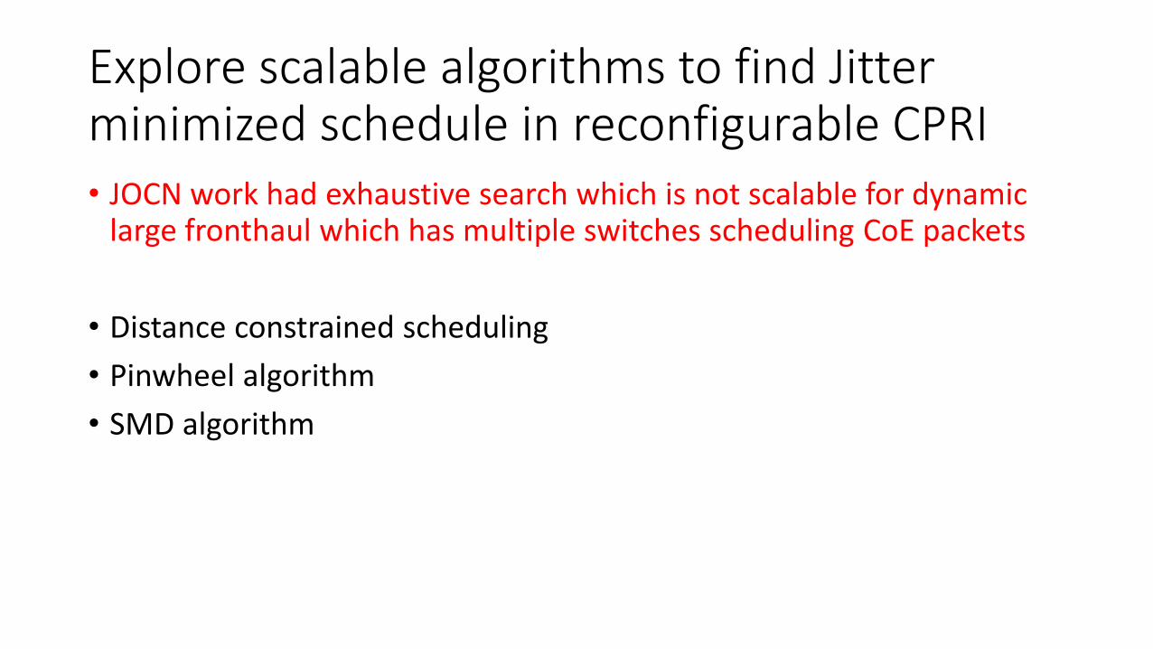
Explore scalable algorithms to find Jitter minimized schedule in reconfigurable CPRI• JOCN work had exhaustive search which is not scalable for dynamic

large fronthaul which has multiple switches scheduling CoE packets

• Distance constrained scheduling

• Pinwheel algorithm

• SMD algorithm

Distance constrained scheduling

• A common approach to scheduling hard real-time tasks with repetitive requests is periodic task model [l], in which each task Ti has a period Pi and an execution time ei

• Ti must be executed once in each of its periods

• Some real-time tasks must be executed in a (temporal) distance-constrained manner, rather than just periodically

• Temporal distance between any two consecutive executions of a task should not be longer than a certain amount of time – within tolerable jitter

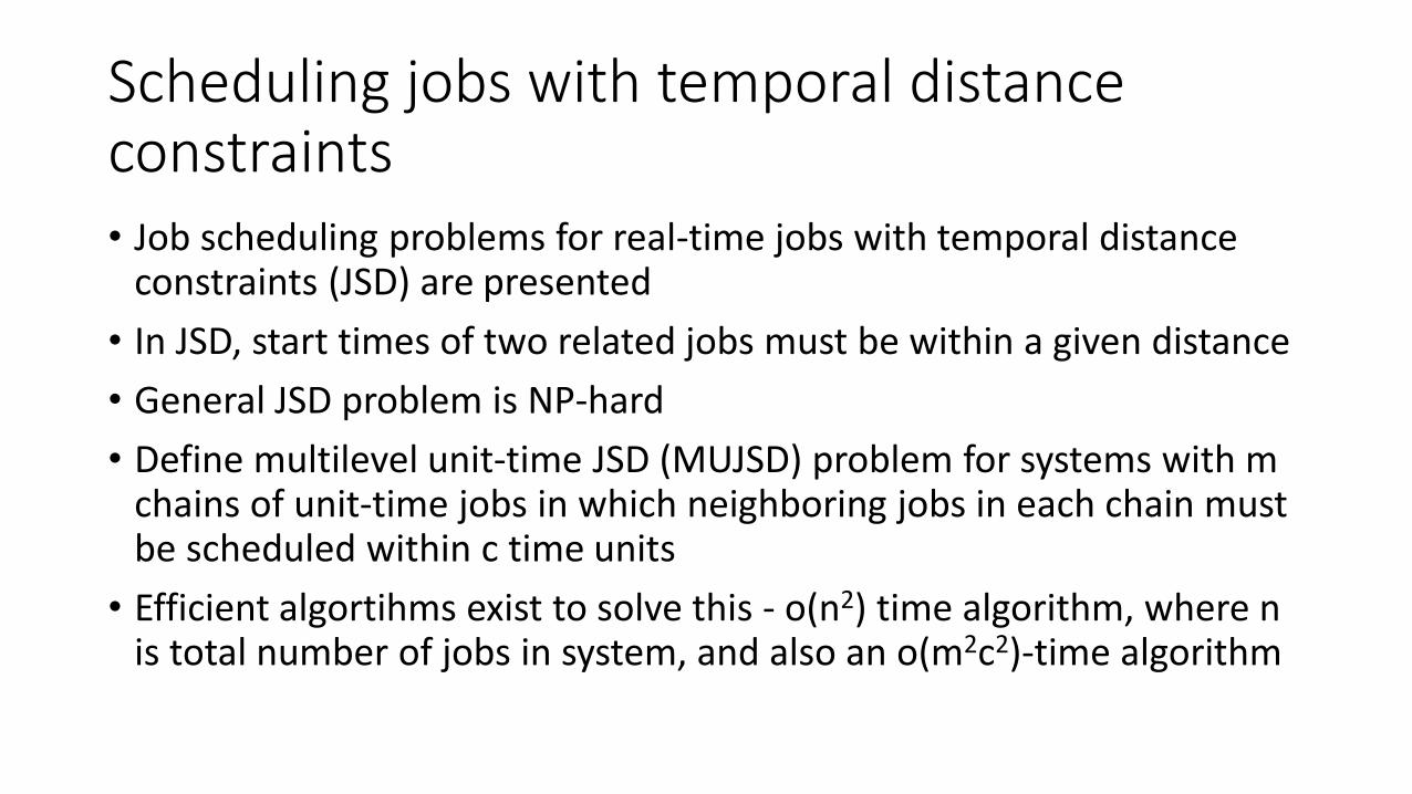
Scheduling jobs with temporal distance constraints• Job scheduling problems for real-time jobs with temporal distance

constraints (JSD) are presented

• In JSD, start times of two related jobs must be within a given distance

• General JSD problem is NP-hard

• Define multilevel unit-time JSD (MUJSD) problem for systems with m chains of unit-time jobs in which neighboring jobs in each chain must be scheduled within c time units

• Efficient algortihms exist to solve this - o(n2) time algorithm, where n is total number of jobs in system, and also an o(m2c2)-time algorithm

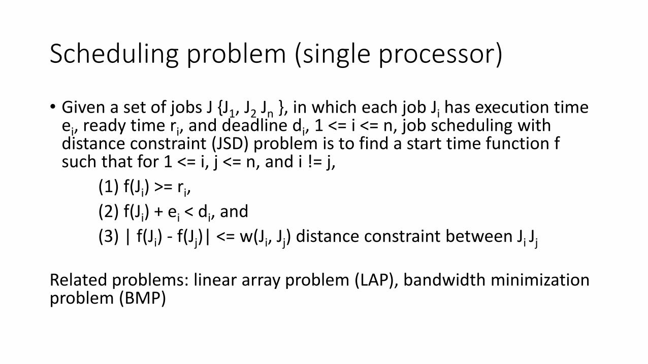
Scheduling problem (single processor)

• Given a set of jobs J {J1, J2 Jn }, in which each job Ji has execution time ei, ready time ri, and deadline di, 1 <= i <= n, job scheduling with distance constraint (JSD) problem is to find a start time function f such that for 1 <= i, j <= n, and i != j,

(1) f(Ji) >= ri,

(2) f(Ji) + ei < di, and

(3) | f(Ji) - f(Jj)| <= w(Ji, Jj) distance constraint between Ji Jj

Related problems: linear array problem (LAP), bandwidth minimization problem (BMP)

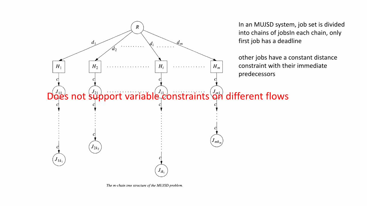
In an MUJSD system, job set is divided into chains of jobsIn each chain, only first job has a deadline

other jobs have a constant distance constraint with their immediatepredecessors

Does not support variable constraints on different flows

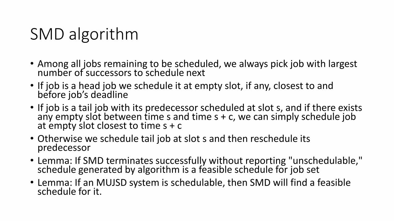
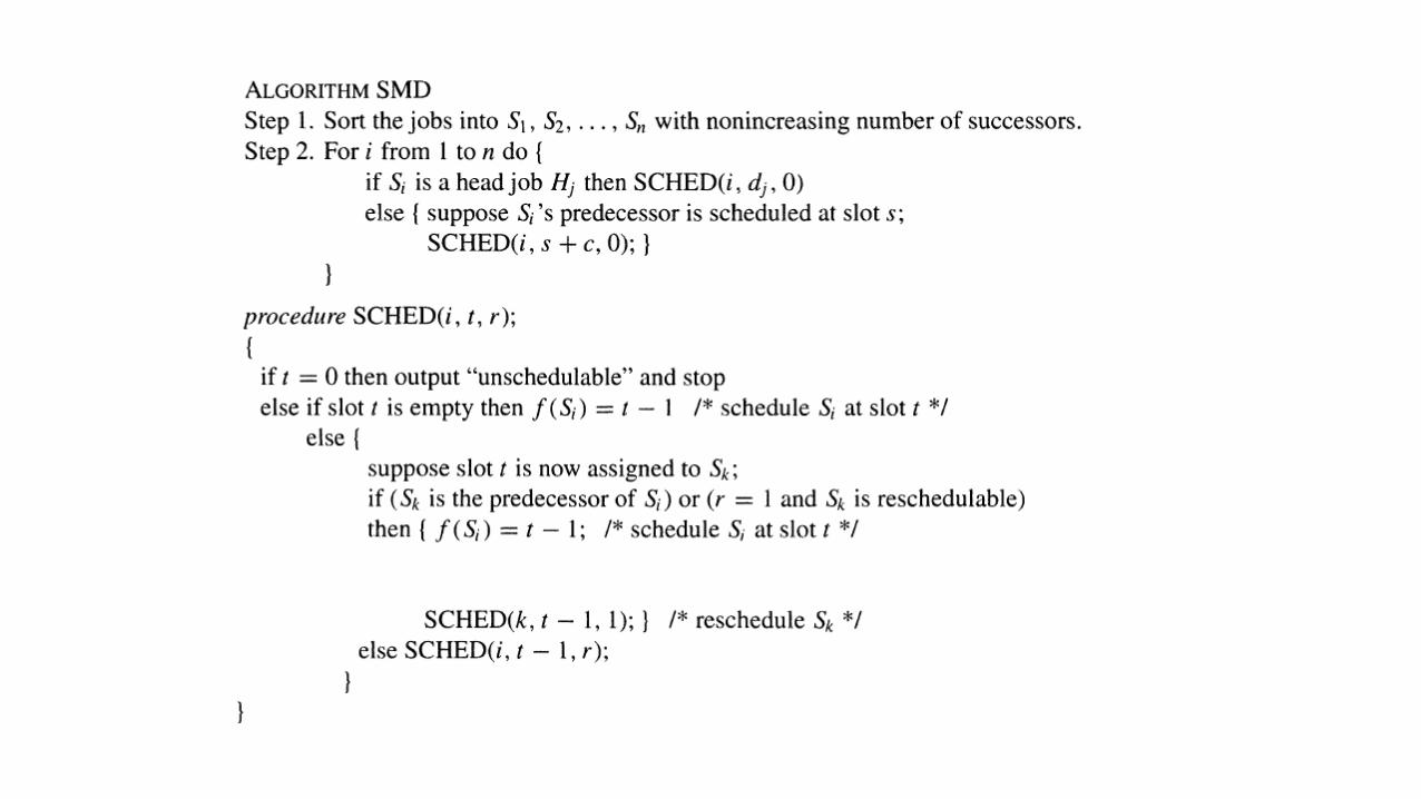
SMD algorithm

• Among all jobs remaining to be scheduled, we always pick job with largest number of successors to schedule next

• If job is a head job we schedule it at empty slot, if any, closest to and before job’s deadline

• If job is a tail job with its predecessor scheduled at slot s, and if there exists any empty slot between time s and time s + c, we can simply schedule job at empty slot closest to time s + c

• Otherwise we schedule tail job at slot s and then reschedule its predecessor

• Lemma: If SMD terminates successfully without reporting "unschedulable," schedule generated by algorithm is a feasible schedule for job set

• Lemma: If an MUJSD system is schedulable, then SMD will find a feasible schedule for it.

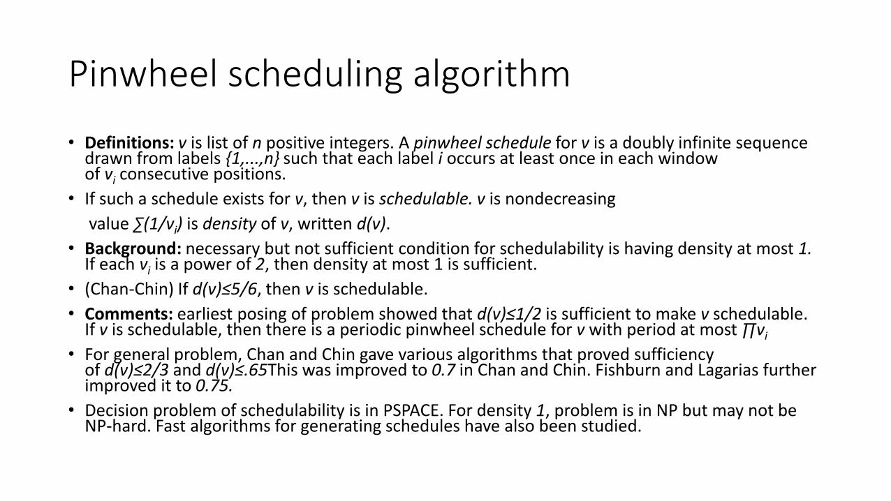
Pinwheel scheduling algorithm

• Definitions: v is list of n positive integers. A pinwheel schedule for v is a doubly infinite sequence drawn from labels {1,...,n} such that each label i occurs at least once in each window of vi consecutive positions.

• If such a schedule exists for v, then v is schedulable. v is nondecreasing

value ∑(1/vi) is density of v, written d(v).

• Background: necessary but not sufficient condition for schedulability is having density at most 1. If each vi is a power of 2, then density at most 1 is sufficient.

• (Chan-Chin) If d(v)≤5/6, then v is schedulable.

• Comments: earliest posing of problem showed that d(v)≤1/2 is sufficient to make v schedulable. If v is schedulable, then there is a periodic pinwheel schedule for v with period at most ∏vi

• For general problem, Chan and Chin gave various algorithms that proved sufficiency of d(v)≤2/3 and d(v)≤.65This was improved to 0.7 in Chan and Chin. Fishburn and Lagarias further improved it to 0.75.

• Decision problem of schedulability is in PSPACE. For density 1, problem is in NP but may not be NP-hard. Fast algorithms for generating schedules have also been studied.

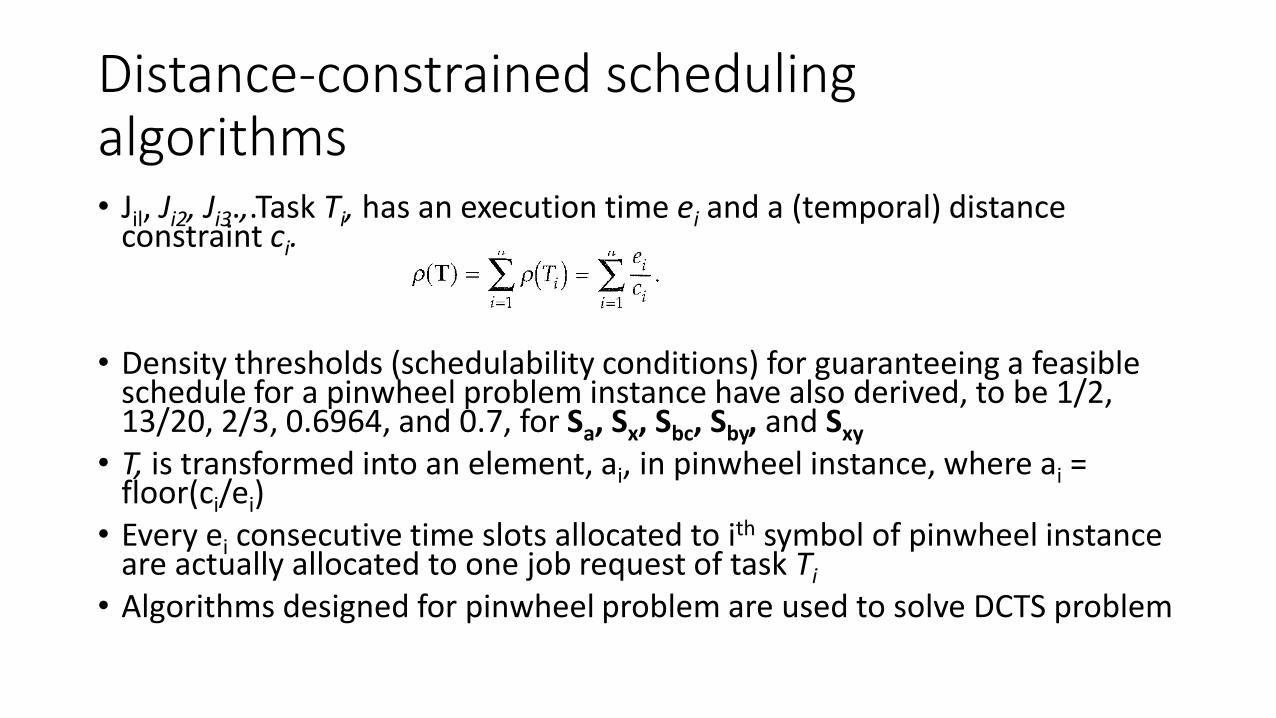
Distance-constrained schedulingalgorithms• Jil, Ji2, Ji3.,.Task Ti, has an execution time ei and a (temporal) distance

constraint ci.

• Density thresholds (schedulability conditions) for guaranteeing a feasible schedule for a pinwheel problem instance have also derived, to be 1/2, 13/20, 2/3, 0.6964, and 0.7, for Sa, Sx, Sbc, Sby, and Sxy

• T, is transformed into an element, ai, in pinwheel instance, where ai = floor(ci/ei)

• Every ei consecutive time slots allocated to ith symbol of pinwheel instance are actually allocated to one job request of task Ti

• Algorithms designed for pinwheel problem are used to solve DCTS problem

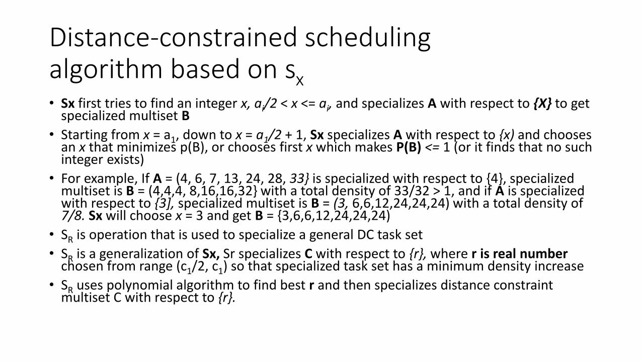
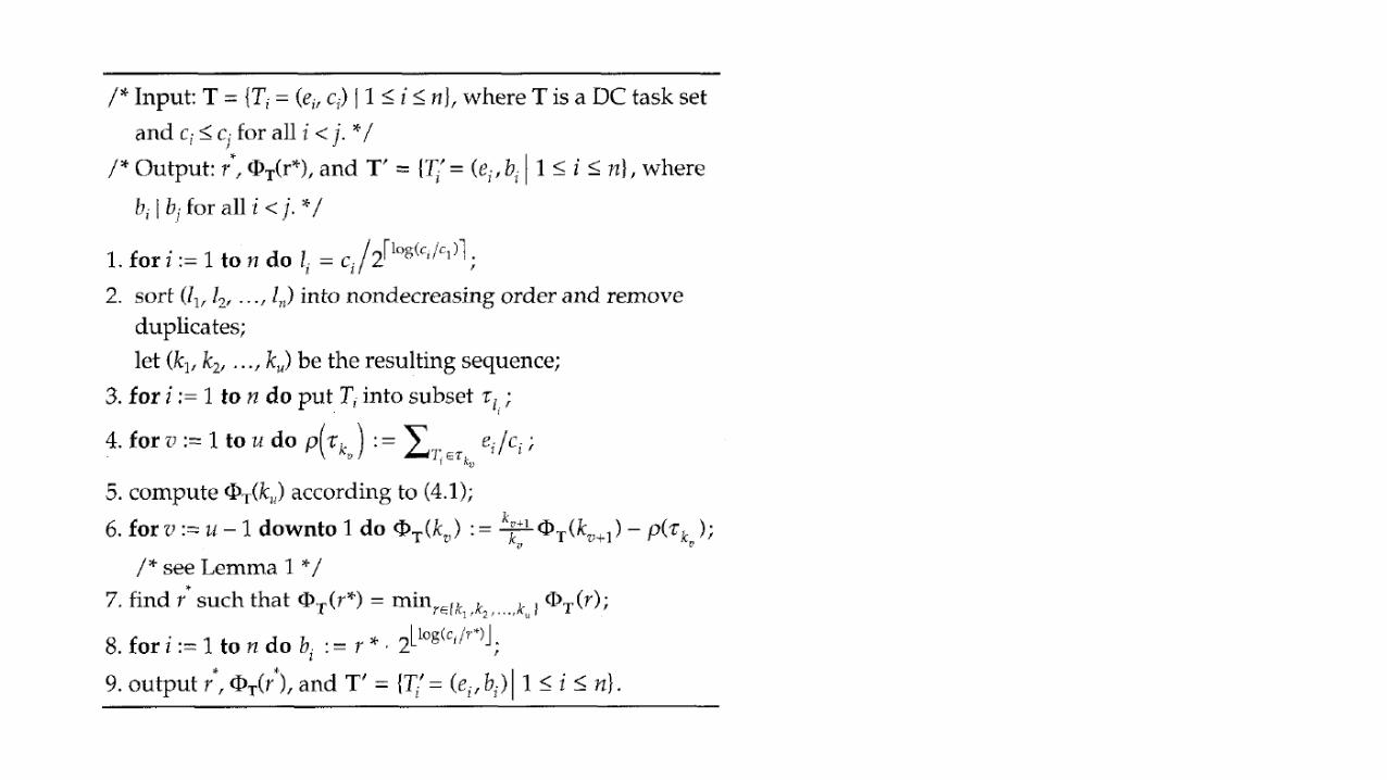
Distance-constrained schedulingalgorithm based on sx• Sx first tries to find an integer x, ai/2 < x <= ai, and specializes A with respect to {X} to get

specialized multiset B

• Starting from x = a1, down to x = a1/2 + 1, Sx specializes A with respect to {x) and chooses an x that minimizes p(B), or chooses first x which makes P(B) <= 1 (or it finds that no such integer exists)

• For example, If A = (4, 6, 7, 13, 24, 28, 33} is specialized with respect to {4}, specialized multiset is B = (4,4,4, 8,16,16,32} with a total density of 33/32 > 1, and if A is specialized with respect to {3], specialized multiset is B = (3, 6,6,12,24,24,24) with a total density of 7/8. Sx will choose x = 3 and get B = {3,6,6,12,24,24,24)

• SR is operation that is used to specialize a general DC task set

• SR is a generalization of Sx, Sr specializes C with respect to {r}, where r is real number chosen from range (c1/2, c1) so that specialized task set has a minimum density increase

• SR uses polynomial algorithm to find best r and then specializes distance constraint multiset C with respect to {r}.

Scheduling algorithms

• Scheduler Sr can schedule task sets with temporal distance constraints.• Distance-constrained task set with n tasks can be feasibly scheduled by

using Scheduler Sr as long as its total density is less than or equal to n(21/n

– 1)• Deterministic guarantee that all tasks will meet their deadlines as long as

total density is held within density threshold• If total density of a DC task set after specialization is less than or equal to 1,

DC task set can be feasibly scheduled by Scheduler Sr• Sr supports scheduling variable flow constraints required for Jitter

minimization in fronthaul• Multiprocessor scheduling will be explored to form schedules for large

number of switches in fronthaul

References

• Chan, MY.; Chin, Francis; Schedulers for larger classes of pinwheel instancesAlgorithmica9 (1993), no5, 425--462

• Mee Yee Chan, Francis YLChin; General schedulers for pinwheel problem based on double-integer reduction, IEEE Transactions on Computers, 41 (1992), 755--768

• Fishburn, PC.; Lagarias, JC.; Pinwheel scheduling: achievable densitiesAlgorithmica 34 (2002), 14--38

• Holte, Robert; Mok, A; Rosier, Louis; Tulchinsky, Igor; Varvel, Donald; pinwheel: A scheduling problem, Proc22nd Hawaii IntlConfSystems Sci., (1989), 693-702

• Holte, Robert; Rosier, Louis; Tulchinsky, Igor; Varvel, Donald; Pinwheel scheduling with two distinct numbersMathematical foundations of computer science 1989 (Por\polhkabka-Kozubnik, 1989), 281--290, Lecture Notes in ComputSci., 379, Springer, Berlin, 1989, and TheoretComputSci100 (1992), no1, 105--135

• Lin, Shun-Shii; Lin, Kwei-Jay; A pinwheel scheduler for three distinct numbers with a tight schedulability boundAlgorithmica 19 (1997), no4, 411--426

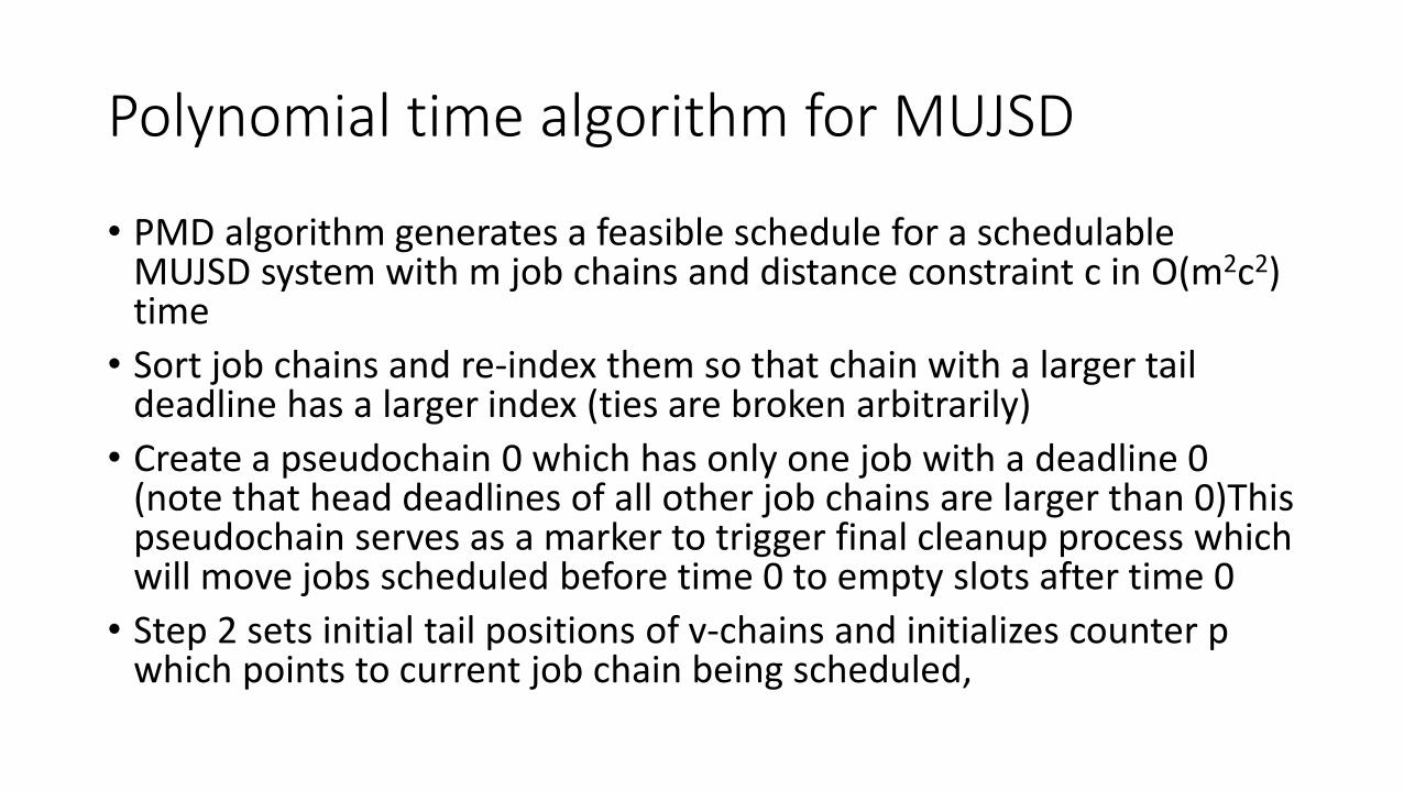
Polynomial time algorithm for MUJSD

• PMD algorithm generates a feasible schedule for a schedulable MUJSD system with m job chains and distance constraint c in O(m2c2) time

• Sort job chains and re-index them so that chain with a larger tail deadline has a larger index (ties are broken arbitrarily)

• Create a pseudochain 0 which has only one job with a deadline 0 (note that head deadlines of all other job chains are larger than 0)This pseudochain serves as a marker to trigger final cleanup process which will move jobs scheduled before time 0 to empty slots after time 0

• Step 2 sets initial tail positions of v-chains and initializes counter p which points to current job chain being scheduled,

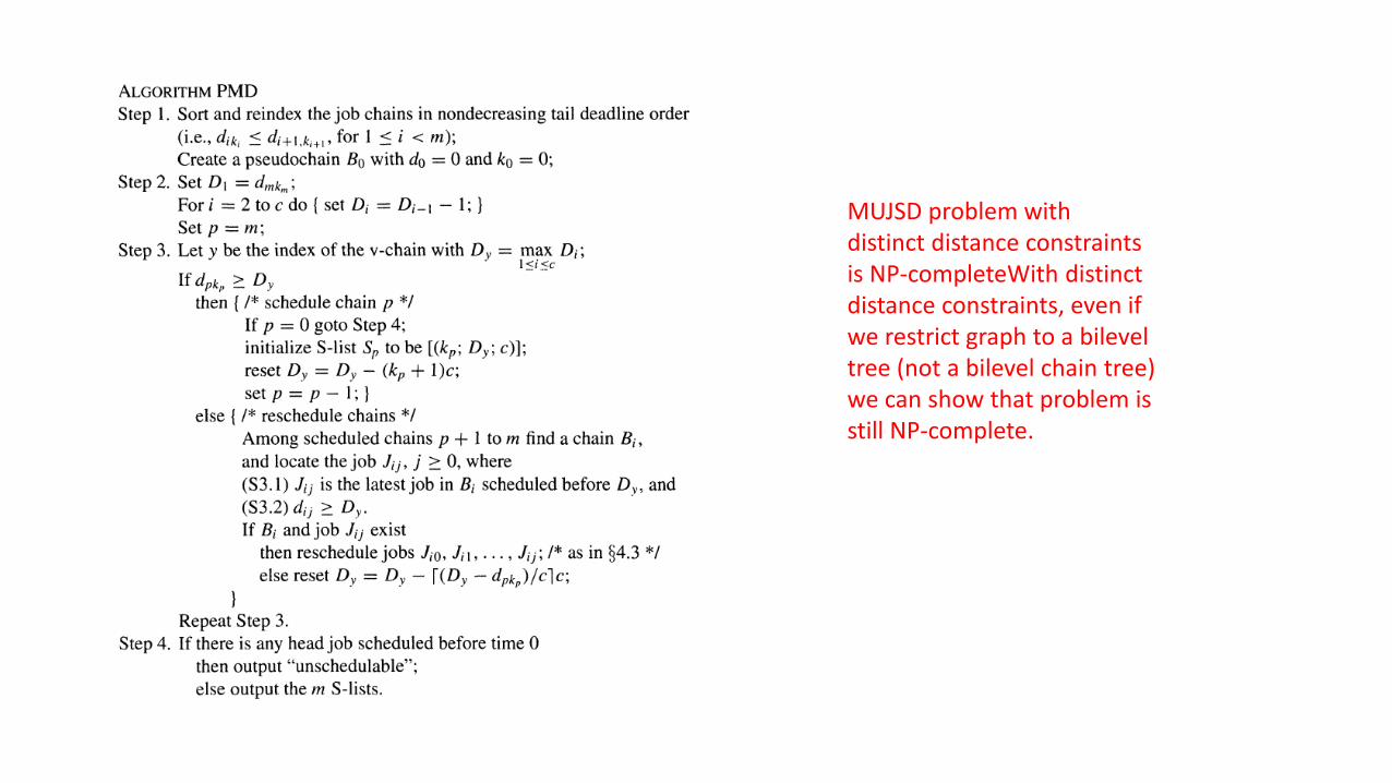
MUJSD problem withdistinct distance constraints is NP-completeWith distinct distance constraints, even if we restrict graph to a bileveltree (not a bilevel chain tree) we can show that problem isstill NP-complete.