Embed Size (px)
Citation preview

Department of Energy and Environment Institute of Aircraft Design
CHALMERS UNIVERSITY OF TECHNOLOGY UNIVERSITY OF STUTTGART
Gothenburg, Sweden 2015 Stuttgart, Germany 2015
SCADA-Data Analysis for Condition
Monitoring of Wind Turbines
Master’s thesis in Energy Engineering
Simon Letzgus


MASTER’S THESIS
SCADA Data Analysis for Condition Monitoring of Wind Turbine Components
Master’s Thesis within the Energy Engineering program
SIMON LETZGUS
EXAMINERS:
Prof. Dr. Po-Wen Cheng Ph.D. Jimmy Ehnberg
SUPERVISORS:
Lic. Pramod Bangalore Dipl. Ing. Kolja Müller
Department of Energy and Environment
Division of Electric Power Engineering
CHALMERS UNIVERSITY OF TECHNOLOGY
Gothenburg, Sweden 2015
Institute of Aircraft Design
Stuttgart Wind Energy (SWE)
UNIVERSITY OF STUTTGART
Stuttgart, Germany 2015


V
Abstract
Wind energy, the world’s fastest growing renewable energy technology, is developing
towards a major utility source. Turbines are growing in size and are located in more
remote sites, sometimes even offshore, to benefit from better wind conditions. These
developments help to maximize the output per turbine but come with challenges for
operation and maintenance (O&M). Unexpected failures result in longer downtimes and
consequently higher revenue losses. Hence, maintenance management promises consid-
erable cost saving potential and the analysis of data form the turbine inbuilt supervisory
control and data acquisition (SCADA) system can effectively support maintenance de-
cisions.
This thesis aims to investigate possibilities to utilize SCADA data for early failure de-
tection in critical wind turbines (WTs). Therefore, a condition monitoring approach is
further developed and applied. The method uses artificial neural networks to model tar-
get parameters under normal operating conditions and analyzes deviations from the
measured values with the help of statistical tools, such as the Mahalanobis distance
(MHD) measure. In order to increase the robustness and accuracy of the approach, the
development of several data pre-processing methods is presented. Two different anoma-
ly detection philosophies are investigated by building two different models. A gearbox
model which is monitoring local variables to indicate component malfunctions and a
power model which is predicting the turbine’s power output to indicate problems form a
system’s perspective.
Based on the available data both monitoring approaches were applied to investigate
gearbox failures for indirect drive WTs and generator bearing failures for direct drive
WTs. Furthermore, the power model was found to be an effective method for ice detec-
tion on WT blades. The successful detection of gearbox anomalies long before a final
component breakdown is presented. However, the model was not able to detect all gear-
related problems investigated. It was concluded that the availability of parameters
which are potentially affected by component malfunctions play a decisive role in this
approach. The power model application showed that a different anomaly detection ap-
proach might be better suited for the investigated cases. However, this approach is well
suited for the detection of icing and recommendations for further studies are derived.
Keywords: Artificial neural networks (ANN), condition monitoring, supervisory con-
trol and data acquisition (SCADA), failure detection, wind power, gearbox monitoring,
turbine monitoring, icing detection

VI
Zusammenfassung
Windenergie, die am schnellsten wachsende Technologie unter den erneuerbaren Ener-
gien, gewinnt weltweit an Bedeutung. Immer größere Anlagen werden an teilweise un-
zugänglichen Orten, beispielsweise Offshore, errichtet, um von guten Windbedingungen
zu profitieren und Energieerträge zu maximieren. Diese Entwicklung bringt jedoch Her-
ausforderungen für Betrieb und Wartung der Anlagen mit sich. Eine intelligente, kos-
tenminimale Wartungsstrategie ist daher besonders wichtig. Die Analyse der Daten aus
dem SCADA-System der Windkraftanlagen kann hierbei wertvolle Informationen zur
Unterstützung der Wartungsplanung liefern.
Im Rahmen dieser Arbeit werden Möglichkeiten zur Nutzung von SCADA-Daten für
die Fehlerfrüherkennung in Windkraftanlagen untersucht. Hierbei wird eine Monitoring
Methode weiterentwickelt und angewendet, die mithilfe von Neuronalen Netzen Anla-
genparameter unter Normalbedingungen modelliert und Abweichungen von gemesse-
nen Werten durch den Einsatz statistischer Methoden, wie beispielsweise der Mahala-
nobis Distanz, untersucht. Hierbei wird der Ansatz zum einen für das Monitoring einer
einzelnen Komponente und zum anderen für die Überwachung der kompletten Anlage
angewendet. Des Weiteren werden, um die Genauigkeit und Robustheit des Ansatzes zu
erhöhen, mehrere Methoden zur Daten-Aufbereitung vorgestellt.
Basierend auf den vorhandenen Daten konzentriert sich die Entwicklung und Anwen-
dung des komponentenbezogenen Ansatzes auf das Getriebe der Windkraftanlagen. Die
Analyse mehrerer Fehlerfälle zeigt, dass die Methode Getriebefehler, lange bevor diese
in einem kompletten Getriebeschaden resultieren, erkennen kann. Im Rahmen des Sys-
tem-Ansatzes wird die Anlagenperformance überwacht. Die Anwendung auf Anlagen
mit Fehlern in der Generator-Lagerung zeigt vor allem die Herausforderungen bei der
Beurteilung von Performance-Abweichungen. Des Weiteren wird gezeigt, dass mit die-
sem Ansatz Eisbildung an den Rotorblättern nachgewiesen werden kann.

VII
Acknowledgement
This research work has been carried out with support through the Professor Dr.-Ing.
Erich Müller-Stiftung. The financial support is gratefully acknowledged.
I would like to sincerely acknowledge my gratitude to my supervisor Pramod Banga-
lore, who has made my stay at Chalmers possible and has supported me throughout the
research project.
I would also like to thank both of my examiners Prof. Po Wen Cheng and Jimmy
Ehnberg as well as my supervisor at my home institute Kolja Müller for their support
and the uncomplicated arrangement of the research exchange.
Special thanks goes to the employees of the industrial partner Stena Renewables; espe-
cially to Thomas Svensson and Johannes Lundvall whose support through data and ex-
pertise in wind turbine operation has contributed substantially to the outcomes of this
work.
Furthermore, I want to thank Daniel Karlsson for the vivid discussions around the
common topic; Tobias Zengel, Sumit Kumar and especially Fabian Hufgard for proof-
reading parts of my report; and in addition all the fellow master thesis students for hav-
ing made the time in the office a good memory.
Finally, I would like to thank Katarzyna Leszek for the warm support during these last
busy weeks and my family for their loving support throughout my studies.
Stuttgart, 2015-08-11

VIII

IX
Declaration of Originality
I hereby certify that I am the sole author of this thesis and that no part of this thesis has
been published or submitted for publication.
Furthermore, I certify that, to the best of my knowledge, my thesis does not infringe
upon anyone’s copyright nor violate any proprietary rights and that any ideas, tech-
niques, quotations, or any other material from the work of other people included in my
thesis, published or otherwise, are fully acknowledged in accordance with the standard
referencing practices.
Stuttgart, 2015-08-11

X

XI
Table of Content
Abstract ........................................................................................................................... V
Zusammenfassung ........................................................................................................ VI
Acknowledgement ....................................................................................................... VII
Declaration of Originality ............................................................................................ IX
Table of Content ............................................................................................................ XI
Preface ........................................................................................................................... XV
List of Figures ............................................................................................................. XVI
List of Tables ........................................................................................................... XVIII
Abbreviations ............................................................................................................... XX
1 Introduction ......................................................................................................... 1
1.1 Background ............................................................................................................ 1
1.2 Task Description .................................................................................................... 2
1.3 WT Data and Project Partner ................................................................................. 2
2 Theoretical Background ..................................................................................... 3
2.1 Wind Turbines and SCADA .................................................................................. 3
2.1.1 The SCADA system .............................................................................................. 4
2.1.2 Gearbox ................................................................................................................. 5
2.2 Reliability and Maintenance in Wind Turbines ..................................................... 7
2.2.1 Wind Turbine Reliability ....................................................................................... 7
2.2.2 Maintenance Management in Wind Turbines ....................................................... 9
2.2.3 Condition Monitoring in Wind Turbines ............................................................. 11
2.2.4 SCADA based CM using Normal Behavior Models ........................................... 13
2.3 Artificial Neural Networks .................................................................................. 14
2.3.1 Building blocks of the Artificial Neural Network ............................................... 15
2.3.2 Network Training Methods ................................................................................. 17
2.3.3 Application of Artificial Neural Networks in Wind Turbines ............................. 19
2.3.4 Neural Networks in MATLAB ............................................................................ 20
2.4 Statistical Background ......................................................................................... 21
2.4.1 Basic Statistical Measures ................................................................................... 21
2.4.2 Distributions ........................................................................................................ 22
2.4.3 Mahalanobis Distance ......................................................................................... 25

XII
2.5 Gearbox Condition Monitoring Approach ........................................................... 26
2.5.1 Gearbox Model .................................................................................................... 26
2.5.2 Anomaly Detection Approach ............................................................................. 26
2.5.3 Anomaly Detection Application .......................................................................... 28
3 Model Development ........................................................................................... 29
3.1 Model Development Process ............................................................................... 29
3.2 Parameter selection .............................................................................................. 30
3.3 Model Architecture.............................................................................................. 31
3.4 Data Pre-Processing ............................................................................................. 32
3.5 Model Training .................................................................................................... 33
3.5.1 Training Period and Turbine Individual Networks .............................................. 33
3.5.2 ANN Training ...................................................................................................... 34
3.5.3 Inconsistencies in ANN Training ......................................................................... 34
3.5.4 Lag and Normalization Consideration ................................................................. 36
3.6 Model Evaluation and Validation ....................................................................... 36
3.6.1 Training Evaluation ............................................................................................. 37
3.6.2 Healthy Turbine Application ............................................................................... 37
3.6.3 Faulty Turbine Application .................................................................................. 38
4 Gearbox Model ................................................................................................... 39
4.1 Model Development and Training ....................................................................... 39
4.1.1 Parameter Selection ............................................................................................. 39
4.1.2 Data Pre-Processing ............................................................................................. 43
4.2 Validation and Comparison ................................................................................. 49
4.3 Model Application ............................................................................................... 53
4.3.1 Gearbox Study Case 1 .......................................................................................... 53
4.3.2 Gearbox Study Case 2 .......................................................................................... 58
4.4 Discussion ............................................................................................................ 61
5 Power Model ....................................................................................................... 63
5.1 Model Development and Training ....................................................................... 63
5.1.1 Parameter Selection ............................................................................................. 63
5.1.2 Data Pre-Processing ............................................................................................. 64
5.1.3 Data post-processing ............................................................................................ 67
5.1.4 Model Training .................................................................................................... 67
5.2 Validation and Comparison ................................................................................. 68
5.3 Model Application ............................................................................................... 71
5.3.1 Power Study Case Gearbox Failure ..................................................................... 71
5.3.2 Power Study Case Generator Bearing Failure ..................................................... 73
5.4 Discussion ............................................................................................................ 75

XIII
6 Closure ................................................................................................................ 78
6.1 Summary .............................................................................................................. 78
6.2 Discussion and Conclusions ................................................................................ 78
6.3 Future Work ......................................................................................................... 80
References ...................................................................................................................... 82

XIV

XV
Preface
The Swedish Wind Power Technology Centre (SWPTC) is a research centre for design
of wind turbines. The purpose of the Centre is to support Swedish industry with knowl-
edge of design techniques as well as maintenance in the field of wind power. The re-
search in the Centre is carried out in six theme groups that represent design and opera-
tion of wind turbines; Power and Control Systems, Turbine and Wind loads, Mechanical
Power Transmission and System Optimisation, Structure and Foundation, Maintenance
and Reliability as well as Cold Climate.
This Master’s Thesis was performed within the main project in Theme group 5.
SWPTC’s work is funded by the Swedish Energy Agency, by three academic and thir-
teen industrial partners. The Region Västra Götaland also contributes to the Centre
through several collaboration projects.

XVI
List of Figures
Figure 2-1: Cut-away view of a typical wind turbine (adopted from [9]) ........................... 4
Figure 2-2: Measurements available in a typical SCADA system [4] ................................ 5
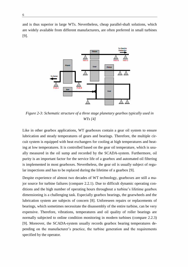
Figure 2-3: Schematic structure of a three stage planetary gearbox typically used in
WTs [4] ........................................................................................................... 6
Figure 2-4: Average number of failures per turbine and year by component and the
resulting downtimes ....................................................................................... 8
Figure 2-5: Contribution of each component to the annual turbine downtime.................... 9
Figure 2-6: ANN based CM approach [4] ......................................................................... 14
Figure 2-7: The sigmoid function plotted with varying shaping parameters .................... 16
Figure 2-8: Examples for different ANN architectures [4] ............................................... 16
Figure 2-9: Normal distribution with different parameter configurations ......................... 23
Figure 2-10: Weibull distribution with different parameter configurations ...................... 24
Figure 2-11: Mahalanobis distances based on a sample (white) with its center (red) ....... 25
Figure 2-12: The averaged MHD violates the threshold several days in advance to a
gearbox bearing failure in [4] ....................................................................... 28
Figure 3-1: Schematic flow chart of the iterative model development process ................ 29
Figure 3-2: Correlation matrix between different SCADA-parameters ............................ 30
Figure 3-3: Example for ‘correct’ prediction of abnormally high bearing temperature
by normal behavior model due to incorrect choice of input parameters ...... 31
Figure 3-4: Turbine specific behavior profile of gear bearing temperatures
throughout a year [4] .................................................................................... 33
Figure 3-5: Bearing temperature measured and modelled with different trainings for
healthy (top) and faulty (bottom) turbine ..................................................... 35
Figure 3-6: Structure of Model Training and Application ................................................ 35
Figure 4-1: Visualization of final gearbox model parameter configuration with inputs
(blue) and targets (violet) ............................................................................. 40
Figure 4-2: Gear bearing temperature depending on power output and rotor rpm ............ 41
Figure 4-3: Gearbox related parameter correlations averaged over more than 10
healthy turbine years .................................................................................... 41
Figure 4-4: Relative performance gear bearing model based on the MSE for different
model input configurations and indication of the model’s anomaly
detection ability. ........................................................................................... 42
Figure 4-5: Visualization of the different filters applied within the gearbox model ......... 44
Figure 4-6: Visualization of the General Boundary Filter ................................................. 45
Figure 4-7: Visualization of the General Cluster Filter ..................................................... 46
Figure 4-8: Temperature overestimation after large data gaps .......................................... 47
Figure 4-9: Visualization of the Skip Filter ....................................................................... 48
Figure 4-10: Performance of different configurations for skip filter and skip
parameter ...................................................................................................... 49
Figure 4-11: Measured versus modelled temperatures for a healthy turbine .................... 50

XVII
Figure 4-12: Training error histogram (100 bins) for the bearing temperature (left)
and the gear oil temperature (right) model .................................................. 51
Figure 4-14a: Gear bearing anomaly detection for healthy turbine .................................. 51
Figure 4-14b: Gear oil anomaly detection for healthy turbine .......................................... 52
Figure 4-15: Modelled and measured temperatures before gearbox failure ..................... 54
Figure 4-16: Anomaly detection of both models before gearbox failure .......................... 55
Figure 4-17: Output versus measured temperatures during the period of model alarm .... 56
Figure 4-18: Rotor RPM and power input signals and SCADA alarms during model
alarm ............................................................................................................ 56
Figure 4-19: Modelled and measured temperatures before gearbox failure ..................... 58
Figure 4-20: Anomaly detection of both models before gearbox failure in SC02 ............ 59
Figure 4-21: ANN input signals and their extreme values in the training data set for
the period when the model triggered alarms ................................................ 60
Figure 5-1: Visualization of final power model parameter configuration with inputs
(blue) and targets (violet) ............................................................................. 64
Figure 5-2: Curtailment data points filtered from a training set. ...................................... 66
Figure 5-3: Big deviation between model output and measured power due to
averaging before and after turbine shutdown. .............................................. 67
Figure 5-4: Measured versus modelled power output in February (left). Training data
(black) and measured power (magenta), right. ............................................ 68
Figure 5-5: Shift of power curve with seasons (left) towards less efficient power
production with lower temperatures (right). ................................................ 69
Figure 5-6: Modelled versus measured turbine power output over one day ..................... 70
Figure 5-7: Power model application for anomaly detection in a gearbox failure case .... 72
Figure 5-8: Modelled versus measured power for three threshold violation periods........ 72
Figure 5-9: Power curve of training and application dataset ............................................ 73
Figure 5-10: Shifted errors during application .................................................................. 73
Figure 5-11: MHD measure for both turbines until failure occurrence ............................ 74
Figure 5-12: Measured values in relation to training data set and model ......................... 75

XVIII
List of Tables
Table 2-1: Overview of CM techniques applied in WTs based on [7] .............................. 11
Table 2-2: Specification of the present gearbox model ..................................................... 26
Table 3-1: ANN architecture specification for all developed models ............................... 32
Table 4-1: Overview of filters of the gearbox model ........................................................ 43
Table 4-2: GBF-boundaries for parameters of the gearbox model .................................... 45
Table 4-3: Specification of parameters for clustering of data set and parameters used
for filtering with MHD ................................................................................. 46
Table 4-4: Model performance for healthy turbine application averaged over 20
ANNs in comparison with literature values. ................................................ 50
Table 4-5: Results of anomaly detection for LSS-bearing failure ..................................... 52
Table 4-6: Summary of gearbox model specifications ...................................................... 53
Table 4-7: Summary of gearbox study case 1 ................................................................... 57
Table 4-8: Summary of gearbox study case two ............................................................... 61
Table 4-9: Overview over investigated gearbox study cases............................................. 62
Table 5-1: Overview of filters of the power model ........................................................... 64
Table 5-2: GBF-boundaries for parameters of the power model ....................................... 65
Table 5-3: Model performance for healthy turbine application averaged over 20
ANNs in comparison with literature values. ................................................ 70
Table 5-4: Summary of power model specifications ......................................................... 71

XIX

Abbreviations
ANN Artificial Neural Network
CBM Condition Based Maintenance
CDF Cumulative Distribution Function
CM Condition Monitoring
COE Cost of Energy
GBF General Boundary Filter
LMA Levenberg-Marquard Algorithm
MAE Mean Average Error
MHD Mahalanobis Distance
MSE Mean Square Error
O&M Operation and Maintenance
PDF Probability Density Function
RMSE Root Mean Square Error
SC Study Case
SCADA Supervisory Control And Data Acquisition
WT Wind Turbine

XXI


1
1 Introduction
1.1 Background
Wind energy is currently the fastest growing renewable generation technology and is an
important pillar for the transition to more sustainable energy systems in many countries.
The global generation capacity reached 370 GW in 2014 which allows a supply of near-
ly 5 % of the world’s electricity demand [1]. In Europe wind is the leading technology
in terms of new power capacity installations, far ahead of conventionals. Today approx-
imately 10 % of the European electricity consumption is generated by wind power and
this share is expected to further grow in the coming years [2]. In other words, wind
power is developing towards a major utility source.
With this massive penetration wind energy has to compete with various generation
technologies and cost of energy (COE) has become an important issue. Therefore, dif-
ferent developments to cut down generation cost can be observed in recent years. Tur-
bine size is increasing steadily to maximize each turbine’s output. In addition, the tur-
bines are erected at sites with best possible wind conditions which are more and more
often found in remote locations, onshore or even offshore. These trends come with new
challenges in O&M. Due to difficult logistics unexpected failures can be costly to repair
and lead to long turbine downtimes, entailing production losses, which can have a sig-
nificant impact on the economics of a project [3].
Hence, maintenance management promises considerable cost saving potential and has
received increasing attention in recent years. Efforts have focused on early failure detec-
tion in critical components of the WT; see for example [4, 5, and 6]. Condition monitor-
ing (CM) concepts provide valuable information and can contribute significantly to in-
creasing turbine reliability. Hence, a smart integration of CM information in the O&M-
strategy, resulting in so called condition based maintenance (CBM), can help to mini-
mize O&M costs. Among the different CM approaches analysis of SCADA data with
appropriate algorithms has shown promising results [4, 7].
The intention of this thesis is to contribute to early failure detection by analyzing data
from the turbine‘s SCADA system. Therefore, the approach presented in [4] will be further
developed and applied to critical WT components.

2
1.2 Task Description
Wind industry has seen rapid growth in recent years with countries striving to have
more sustainable energy sources in the electric power system. One of the obstacles for
the growth of wind industry is high maintenance cost and long downtimes for WTs,
especially for offshore wind farms [8]. Hence, focus on early detection of failure of crit-
ical components in the WT and condition based maintenance has increased in recent
times. Traditional condition monitoring using vibration signals has proven to be a useful
tool for monitoring the health of components. Furthermore, use of information rich Su-
pervisory Control and Data Acquisition (SCADA) data has received increased attention
in recent years. This thesis aims to contribute to early failure detection by analyzing
data from the turbine’s SCADA system.
Within the framework for a wind power maintenance management tool, a methodology
based on artificial neural networks for anomaly detection in gearboxes was presented in
[4]. The gearbox is a critical component of the WT in terms of reliability and the ap-
proach has to be further developed and applied to new turbine data in study cases.
Moreover, the project will analyze the potentials of monitoring the overall turbine per-
formance to detect degradation in one of the subcomponents. In particular, the detection
of generator bearing failures in direct drive turbines is investigated.
1.3 WT Data and Project Partner
This master’s thesis project was carried out in cooperation with Stena Renewable as an
industrial partner. Stena Renewables operates multiple wind farms in Sweden and pro-
vided data extracted from their SCADA systems. Moreover, Stena Renewable contrib-
uted to the project through their expertise in wind farm O&M. The outcome of the pro-
ject relies both on the correct application of appropriate methods as well as the quality
of the input data. Thus the most promising data sets were carefully selected. With the
analysis of the provided data, we hope to be able to contribute to the understanding of
the recorded problems, as well as an early detection of future failures.
In addition, SCADA data was provided from a WT manufacturer for different failure
cases. Unfortunately not much additional information regarding the turbine’s condition
and maintenance activities was available for these data sets. However, the data has been
investigated and conclusions were drawn when possible.

3
2 Theoretical Background
This chapter provides the theoretical background knowledge which is required to un-
derstand and critically discuss the analysis conducted within this master’s thesis.
Therefore, the first chapter gives an introduction into WTs and the relevant components
followed by the chapters focusing on reliability and maintenance in WTs. Furthermore,
the concept of neural networks, the statistical tools used within this thesis and the ap-
proach for anomaly detection in WTs are presented. References are given, when a more
detailed explanation would exceed the scope of the chapter.
2.1 Wind Turbines and SCADA
WTs have long been used to utilize the kinetic energy of the wind. Nowadays mainly
three bladed horizontal axis WTs are used for power generation. The turbines consist of
typical sub components, which are briefly described below (based on [9]):
Rotor: consists of usually three blades flanged to the hub, which is mounted on
the front end of the rotor shaft outside the nacelle. The rotor converts the kinetic
energy of the wind into mechanical energy and transmits the rotation to the
shaft.
Mechanical Drive Train: describes all rotating mechanical components in be-
tween the rotor hub and the generator. Its design can vary significantly depend-
ing on the turbines drive concept. Direct drive turbines are able to operate with-
out the most complex drive train component, the gearbox, but come with special
requirements for the generator. The drive philosophy also influences the shaft
bearing concept.
Electrical System: Covers all components for the conversion of the mechanical
into electrical energy with the generator as the main component. Conventional
synchronous and asynchronous generators can be found in WTs depending on
the grid connection concept. A common configuration is a synchronous genera-
tor in combination with a converter, which decouples the generator and from the
grid.
Nacelle: protects the whole drive train and the electrical system against envi-
ronmental impacts. Can be turned by the yaw system so that the rotor is always
facing the main wind direction. Furthermore, the nacelle contains various auxil-
iary systems such as brakes, cooling system or measuring equipment to ensure a
safe operation.

4
Tower: The whole previously described configuration is mounted on top of a
tower to benefit from higher wind speeds above ground.
Figure 2-1 shows the typical arrangement of the described components.
Figure 2-1: Cut-away view of a typical wind turbine (adopted from [9])
2.1.1 The SCADA system
Contrary to conventional power plants, WTs are unmanned and often situated in remote
locations. Nevertheless, a wind power plant also needs to be controlled and monitored.
Therefore, the turbines are equipped with monitoring and data evaluation systems, so
called Supervisory Control and Data Acquisition (SCADA) systems. On one hand
SCADA enables to remote control the power plant. Turbines can be switched on or off,
power output can be curtailed and the power factor adjusted if necessary. On the other
hand the SCADA system collects measurements of various sensors placed all over the
WT. Technical parameters, such as bearing and lubrication oil temperatures, electric
quantities and power output are measured as well as environmental parameters like
wind speed, wind direction or ambient and nacelle temperature. In fact, each WT manu-
facturer has an individual concept of how to set up the SCADA system of their turbines.
Figure 2-2 gives an overview over the basic measurements typically collected.

5
Figure 2-2: Measurements available in a typical SCADA system [4]
Although highly individual, all of them have in common that large quantities of data are
extracted and stored in databases. Modern turbines store hundreds of data points every
ten minutes, which leads to a tremendous amount of data over the years. A complete
yearly SCADA data set of one of the turbines analyzed in this thesis, for example, con-
tained more than half a million single measurements. Extracting them from the database
for analysis can be time-consuming work, depending on the user-friendliness of the in-
terface and the available hardware.
The collected measurements give an insight into the turbine’s instantaneous operating
conditions and thus enable remote turbine monitoring. The SCADA system is, for in-
stance, able to automatically generate alarms and warnings, if a parameter exceeds a
pre-selected threshold value. However, the information about turbine condition which is
hidden in SCADA data is not fully utilized by turbine operators nowadays. This is par-
tially due to the fact that the system indicates impending failures too late and generates
a vast number of alarms and warnings giving operators a hard time to distinguish be-
tween serious and negligible error messages [4]. Nevertheless, information from
SCADA data can be extracted using more advanced mathematical and statistical meth-
ods.
2.1.2 Gearbox
A gearbox is typically used to increase the rotational speed of a WT’s rotor in order to
utilize it for a higher speed electrical generator. Modern gearboxes can perform gear
ratios of more than 1:100 and lose only a few percent of the transmitted power [9].
There are two main forms of toothed-wheel gearboxes: parallel-shaft systems and the
technically more advanced planetary gearing. WTs generally require multiple stage gear
systems and combined planetary-parallel-system can be found (compare Figure 2-3).
The integrated planetary solution shows clear advantages in size, mass and relative cost
6
and is thus superior in large WTs. Nevertheless, cheap parallel-shaft solutions, which
are widely available from different manufacturers, are often preferred in small turbines
[9].
Figure 2-3: Schematic structure of a three stage planetary gearbox typically used in
WTs [4]
Like in other gearbox applications, WT gearboxes contain a gear oil system to ensure
lubrication and steady temperatures of gears and bearings. Therefore, the multiple cir-
cuit system is equipped with heat exchangers for cooling at high temperatures and heat-
ing at low temperatures. It is controlled based on the gear oil temperature, which is usu-
ally measured in the oil sump and recorded by the SCADA-system. Furthermore, oil
purity is an important factor for the service life of a gearbox and automated oil filtering
is implemented in most gearboxes. Nevertheless, the gear oil is usually subject of regu-
lar inspections and has to be replaced during the lifetime of a gearbox [9].
Despite experience of almost two decades of WT technology, gearboxes are still a ma-
jor source for turbine failures (compare 2.2.1). Due to difficult dynamic operating con-
ditions and the high number of operating hours throughout a turbine’s lifetime gearbox
dimensioning is a challenging task. Especially gearbox bearings, the gearwheels and the
lubrication system are subjects of concern [8]. Unforeseen repairs or replacements of
bearings, which sometimes necessitate the disassembly of the entire turbine, can be very
expensive. Therefore, vibrations, temperatures and oil quality of roller bearings are
normally subjected to online condition monitoring in modern turbines (compare 2.2.3)
[9]. Moreover, the SCADA-system usually records gearbox bearing temperatures de-
pending on the manufacturer’s practice, the turbine generation and the requirements
specified by the operator.

7
2.2 Reliability and Maintenance in Wind Turbines
As shown in the previous sections, WTs contain conventional components and subas-
semblies of mechanical-electrical energy conversion, such as a shafts, bearings, gear-
boxes and generators. Like other technical systems, they have to undergo regular ser-
vice to guarantee their correct operation. Nevertheless, maintenance is particularly im-
portant for a wind power plant, because WTs have to stand harsh environmental condi-
tions where component failures can have a decisive impact on a project’s economic suc-
cess. The following sections will provide information about the reliability of modern
turbines and highlight the current state-of-art in WT O&M.
2.2.1 Wind Turbine Reliability
Once a WT is commissioned it has to operate properly for a design lifetime of at least
20 years. Unlike other technical systems the turbines operate for several thousand hours
each year while being exposed to a wide range of wind speeds and temperatures, includ-
ing extreme weather situations such as storms, lightning strikes and hail [9]. In fact, the
site location has a significant impact on turbine reliability through the prevailing climate
[10].These rough environmental conditions result in heavy dynamic loads, making WT
components prone to fatigue failures. In consequence, reliable turbine design and opera-
tion is a challenging task [9].
On a system level, reliability is often characterized by turbine availability which is
calculated by dividing the mean time to failure MTTF through the sum out of MTTF and
the mean down time MDT (compare equation 2-1)
(2-1)
Despite the rough operating conditions average availability of today’s onshore turbines
is usually above 95 % [11]. However, this high availability can only be guaranteed by a
costly maintenance organization [12].
When analyzing turbine reliability in greater detail, it has been observed that some
components of a WT fail more frequently than others, indicating that they are particu-
larly sensitive. The frequency of a specific failure’s occurrence is typically reported as
its average failure rate as failure per turbine and year. Therefore, the absolute
number of failures which occurred in a specific component is summed up over a
certain period and then divided by the observation time in turbine years (compare
equation 2-2) [13].
(2-2)

8
However, reliability of a turbine cannot be judged by looking at the failure frequency
only, because the measure does not indicate the severity of a failure. Therefore, the
average downtime per failure caused by a specific component is calculated by
summing up the individual downtimes and dividing them by the total number of
observed failures (compare equation 2-3) [13]. The result is a measure for the aver-
age severity and production loss related to a certain component’s failure.
(2-3)
Both measures, the average failure frequency of a component and the average down-
time of such a failure, are combined to calculate the average annual downtime caused
by the turbine component, which indicates the severity of a failure and corresponds to
the lost revenue due to a malfunction. This number is suggested as an indirect indica-
tor for the economic damage of a failure, in case no financial information is available
[5].
In this thesis, data presented in [14] containing data for more than 620 turbines be-
tween 1997 and 2005 as well as data from a database containing 28 additional WTs with
more actual data was used for the analysis of turbine reliability. Together, the data rep-
resents almost 3200 years of turbine operation. All of the turbines are located in Sweden
and their size ranges from several hundred kW up to multiple MW. The results are pre-
sented in Figure 2-4 in form of average number of failures per turbines and year
grouped by components and their subsequent average downtimes:
Figure 2-4: Average number of failures per turbine and year by component and the
resulting downtimes
The highest failure rate can be found in electrical components, the control system,
including sensors, and the hydraulic system. However, these failures can often be
9
fixed by a simple restart of the turbine system whereas other components cause much
longer downtimes due to repair work and maintenance logistics. Breakdowns of main
turbine components can lead to standstill periods of several weeks. That is why par-
ticularly gearbox failures cause long downtimes even though their average failure rate
is not exceptionally high.
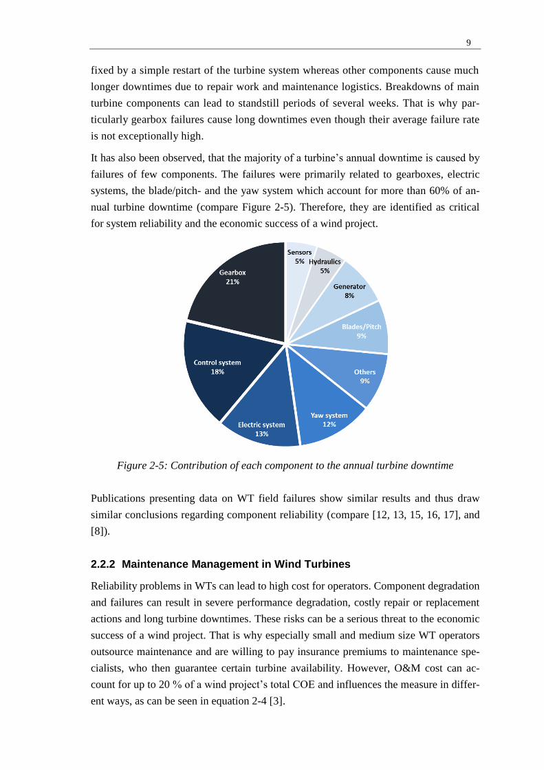
It has also been observed, that the majority of a turbine’s annual downtime is caused by
failures of few components. The failures were primarily related to gearboxes, electric
systems, the blade/pitch- and the yaw system which account for more than 60% of an-
nual turbine downtime (compare Figure 2-5). Therefore, they are identified as critical
for system reliability and the economic success of a wind project.
Figure 2-5: Contribution of each component to the annual turbine downtime
Publications presenting data on WT field failures show similar results and thus draw
similar conclusions regarding component reliability (compare [12, 13, 15, 16, 17], and
[8]).
2.2.2 Maintenance Management in Wind Turbines
Reliability problems in WTs can lead to high cost for operators. Component degradation
and failures can result in severe performance degradation, costly repair or replacement
actions and long turbine downtimes. These risks can be a serious threat to the economic
success of a wind project. That is why especially small and medium size WT operators
outsource maintenance and are willing to pay insurance premiums to maintenance spe-
cialists, who then guarantee certain turbine availability. However, O&M cost can ac-
count for up to 20 % of a wind project’s total COE and influences the measure in differ-
ent ways, as can be seen in equation 2-4 [3].

10
(2-4)
ICC represents the initial capital cost, usually the most important factor in the equa-
tion, which is multiplied with the fixed charge rate (FCR) and added to the levelized
replacement cost (LRC), which is determined by turbine reliability. Moreover, reliabil-
ity influences the COE directly through O&M costs as well as indirectly by affecting
the Annual Energy Production (AEP), which can be severely affected by failure
caused downtime. Therefore, reducing reliability related costs shows great overall cost
reduction potential and maintenance management aims to determine the optimal
maintenance strategy to minimize these costs [3].
In maintenance management two main strategies can be distinguished and goal of intel-
ligent maintenance management is to identify a cost optimal strategy between those two
traditional approaches [7] (compare Figure 2-1).
Figure 2-1: Costs associated with traditional maintenance strategies (Adopted from
[7])
Corrective, sometimes also called reactive maintenance is a run to failure con-
cept. Maintenance actions are initiated after failure occurrence and detection.
Thus, cost of repair is potentially high as only minimal failure prevention efforts
are made. Also, this concept can lead to long turbine downtimes, in case compo-
nents with a long lead time need to be replaced. However, a corrective mainte-
nance approach allows utilizing the component lifetime to its maximum.
Preventive maintenance on the other hand intends to prevent an equipment
breakdown through regular scheduled maintenance or condition based mainte-
Number of Failures
To
tal M
ain
ten
an
ce
Co
st
Total Cost
Prevention Cost
Repair Cost
Corrective
Maintenance
Preventive
Maintenance
optimum
Intelligent
Maintenance
11
nance (CBM) actions. CBM is a subcategory of preventive maintenance which
takes additional information about the turbine components into account. With
the knowledge about the component’s condition actions can be initiated to miti-
gate the consequences of a failure even before failure occurrence. Therefore, it is
necessary to detect the change in machinery condition on time and to be able to
interpret the observed change correctly [18]. However, preventive maintenance
aims for a reduction of repair cost which is partially compensated by the increas-
ing prevention efforts.
2.2.3 Condition Monitoring in Wind Turbines
For successful maintenance management, information about the turbine condition is
essential. Based on that, the appropriate maintenance actions can be arranged. Tradi-
tionally, the information was acquired through manual onsite inspections. However,
with the increasing number of installed turbines in remote sites frequent inspections
becomes more challenging and expensive. Therefore, new CM-strategies are developed,
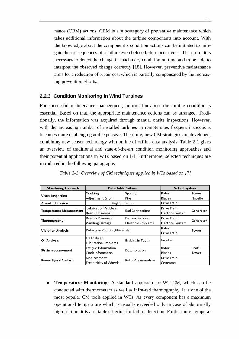
combining new sensor technology with online of offline data analysis. Table 2-1 gives
an overview of traditional and state-of-the-art condition monitoring approaches and
their potential applications in WTs based on [7]. Furthermore, selected techniques are
introduced in the following paragraphs.
Table 2-1: Overview of CM techniques applied in WTs based on [7]
Temperature Monitoring: A standard approach for WT CM, which can be
conducted with thermometers as well as infra-red thermography. It is one of the
most popular CM tools applied in WTs. As every component has a maximum
operational temperature which is usually exceeded only in case of abnormally
high friction, it is a reliable criterion for failure detection. Furthermore, tempera-
Monitoring Approach
Visual InspectionCracking
Adjustment Error
Spalling
Fire
Rotor
Blades
Tower
Nacelle
Acoustic Emission
Temperature Measurement Lubrication Problems
Bearing DamagesBad Connections
Drive Train
Electrical SystemGenerator
ThermographyBearing Damages
Winding Damage
Broken Sensors
Electrical Problems
Drive Train
Electrical SystemGenerator
Vibration AnalysisRotor
Drive TrainTower
Oil AnalysisOil Leakage
Lubrication ProblemsBraking in Teeth
Strain measurementFatigue Information
Crack InformationDeterioration
Rotor
Blades
Shaft
Tower
Power Signal AnalysisDisplacement
Eccentricity of WheelsRotor Assymmetries
WT subsystem
Drive Train
Detectable Failures
High Vibration
Drive Train
Generator
Gearbox
Defects in Rotating Elements

12
tures are rather slow changing measurements due to the thermal inertia of the
components. This can be an advantage when analyzing data with a low sample
rate, for example 10 minute average values stored in a SCADA system. For
temperature this can be a sufficient resolution for condition monitoring. On the
other hand, slow changing measures have only limited value in early failure pre-
diction because they simply indicate a failure too late. Nevertheless, tempera-
tures are often used as a secondary criterion in case, for example, the vibration
monitoring shows an alarm.
Vibration Monitoring: One of the well-established technologies for rotating
machinery is the analysis of vibration signals, since changes in mechanical
equipment can lead to abnormal vibration signals long before a failure occurs.
The vibration signals, recorded by different sensors, are usually transformed into
a frequency domain and then analyzed. In WTs vibration analysis is applied to
monitor shafts, bearings, gearboxes and blades. Shortcomings of this technology
are the requirement of additional equipment and difficulties in detecting low-
frequency faults.
Oil Analysis: Another broadly applied monitoring technique, especially in tur-
bines with gearboxes. As shown in 2.2.1, gearboxes are especially critical in
terms of reliability and therefore gear oil analysis commonly used for gearbox
monitoring, as it is the only method for detecting cracks inside the gearbox.
Usually the oil’s viscosity, oxidation, water content, particles and temperature
are recorded either through offline-sample analysis or online monitoring. Even
though modern on-line sensing methods, such as electromagnetic, flow or pres-
sure-drop and optical debris sensing, are available, offline sample monitoring is
often used due to the high cost for the online equipment.
Strain and Optical Monitoring: Recently, strain measurement and optical fiber
monitoring for WT structures has received increasing attention as the fatigue
loads the turbine is exposed to can be estimated. The measurements of strain
gauges, which can be placed randomly on the structure, are processed with the
help of finite element method to monitor the effects of the high dynamic loads.
However, strain gauges are not very long lasting and these techniques require
expensive measurement equipment. New approaches try to connect available
SCADA-data measurements and short term strain measurements to extrapolate
strain estimations. Such applications might help the technology to a broader ap-
plication in the future [19].
The technologies presented in the previous paragraphs are mainly used to monitor a
specific subsystem within the turbine. Other approaches widen the balance limits and
aim for monitoring the global WT system. Different mechanical and electrical faults for

13
example lead to disturbances in the mechanical as well as in the electrical energy flow.
Consequently mechanical torque oscillation can also be detected on the electrical side of
the power train through power signal analysis. That way blade or rotor imbalances can
be detected. A comparably simple method is the monitoring of process parameters.
There, the values and relationships of temperatures, power, wind and rotor speed or
blade angles are compared with specifications and limits determined by manufacturers.
For this kind of analysis for example SCADA-signals can be used. More advanced ap-
proaches based on parameter prediction and trending are not common today.
However, the importance of condition monitoring is expected to further increase in the
future, due to the earlier mentioned developments in the wind industry. The more ma-
ture the new techniques become, the cheaper their application gets. Also, the cost of
condition monitoring can be compensated with lower premiums for insurances reward-
ing such systems [9] Developing towards more reliable, cost effective, integrated and
smart solutions condition monitoring is about to become an integral part of modern
maintenance strategies [7]).
2.2.4 SCADA based CM using Normal Behavior Models
Today’s turbines are not necessarily equipped with sensors for stress, vibration or power
analysis, but with numerous units collecting data for the SCADA system (compare
2.1.1). The SCADA system collects information about the turbine key features, which
can be analyzed for condition monitoring purposes. Thus, the analysis of SCADA data
can be a cost effective integrated way to monitor several critical components of a WT
[5].
Different techniques, ranging from simple threshold checks to complex statistical
analyses are used to detect anomalies. A comprehensive overview of publications and
their proposed methods to analyze SCADA data for CM of WTs is provided by [20].
A common approach is the application of normal behavior models. Based on inputs
extracted from SCADA data the model should be able to predict a target parameter
under normal operating conditions. For anomaly detection the real time signal is com-
pared with the estimated model output. The success of the approach is determined by
the accuracy of the developed model. Here artificial intelligence methods have proven
to be a sufficient tool for modelling complex systems, such as WT components [21].
Among different approaches neural networks showed particularly good results and were
successfully applied in WT fault detection [22].

14
Figure 2-6: ANN based CM approach [4]
However, the utilization of SCADA data for CM comes with some challenges. Since
the SCADA system was not originally designed for CM, not all parameters for a full
turbine CM are available. Also, the data rate of 10 minute average values is too slow
for some condition monitoring techniques [7]. Moreover, it can be difficult to trace
back an anomaly in the data to its origin. Therefore, it is important to understand a
failure’s specific impact on SCADA data. This knowledge can be achieved either
through the analysis of data along with maintenance reports or with the help of data
mining approaches, depending on data availability [21]. Nevertheless, exploitation of
SCADA data for WT condition monitoring has successfully been demonstrated in
several studies; see [4, 5, 6, 21, 23, 24 and 25].
2.3 Artificial Neural Networks
Artificial neural networks (ANN) are a concept of computing inspired by the biologi-
cal structure brain. In analogy an ANN is able to acquire knowledge in a learning pro-
cess. After training it can recall the learned patterns and input/output relations. Since
the training data presented to the ANN can be theoretical, experimental empirical or a
combination of these, ANNs can be used for a broad range of applications [26]. More-
over, the network is able to generalize its knowledge to a certain extent and apply it to
new input data it has never seen before. This makes it a powerful tool, well suited to
model real world non-linear systems in engineering and science [27]. For problems,
which are too complex for an analytical approach, ANNs can deliver an almost perfect
approximation based on the experience drawn from the training data. However, this
lack of analytical background comes with difficulties in explaining and judging the
ANN’s output [26]. Even though the ANN is a black box model, it was demonstrated
to be a useful tool in various applications [27]. The following sections give a general
introduction into structure and functionality of ANNs based on [28].

15
2.3.1 Building blocks of the Artificial Neural Network
The fundamental information processing unit of an ANN is called a neuron. A neuron
generates an output based on its input signals and consists of three basic elements: A set
of synapses, an adder and an activation function (compare Figure 2-2).
Figure 2-2: Model of a neuron [4]
Synapses are characterized by a weight or strength, which is determined during model
training. A neuron’s input signal at synapse j is multiplied with the synaptic weight
. Subsequently, it is added to all other weighted input signals and a fixed bias value
by a linear combiner (compare equation 2-5). This sum is input for the activation
function which determines the neuron’s output then (compare equation 2-6).
(2-5)
(2-6)
There are two different types of activation functions: Threshold and sigmoid functions.
A threshold function is discontinuous and can assume a value of either 0 or 1 whereas a
sigmoid function can assume any value between 0 and 1. Sigmoid functions are well
balanced between linear and nonlinear behavior and the most common activation func-
tions used in neural networks. Their shape can be influenced by variation of the slope
parameter . Note that the sigmoid function becomes a threshold function for an infinite
(compare equation 2-7). Figure 2-7 shows the corresponding graph for different shape
parameters.
(2-7)

16
Figure 2-7: The sigmoid function plotted with varying shaping parameters
Neurons can be arranged in different architectures depending on the network’s purpose.
A single-layer network, as the name suggests, consists of only one single layer of neu-
rons which directly connect inputs and outputs. Multi-layer networks on the other hand
contain one or more hidden layers. Outputs of the previous layer are used as input for
the next layer. The elements of those layers, the hidden neurons, cannot be directly seen
from either input or output of the network. Through hidden layers the network is able to
model the higher order non-linearity in the input output relationship.
In general, feed-forward and recurrent networks can be distinguished. In contrary to a
feed-forward network a recurrent network has at least one feedback loop. Through
feedback loops, non-linear dynamic behavior can be implemented and the performance
of a network can be improved significantly. Figure 2-8 shows examples of different
network structures.
Figure 2-8: Examples for different ANN architectures [4]
-1 -0.8 -0.6 -0.4 -0.2 0 0.2 0.4 0.6 0.8 1
0
0.2
0.4
0.6
0.8
1
x
(
x)
a = infite
a = 100
a = 25
a = 5

17
Neural network design is a challenging task, because of the lack of well-developed the-
ory for network optimization. An architecture which is able to predict with accuracy
must be found through experimental studies for a specific case. Two approaches are
common to find the optimal network structure. The first option is to start with an over-
sized network and remove synapses or entire neurons, if they are not active or carry
only little weight. Starting with a small network and increasing the number of neurons
until satisfactory solutions are achieved is the second option. Both approaches include a
trial and error to find the network, which suits the application best. However, when
modelling real world non-linear relationships generally two hidden layers lead to suffi-
cient results [4].
2.3.2 Network Training Methods
ANNs are intelligent systems, which are able to learn from their environment.
Knowledge about input/output relations is acquired through a learning process and
stored in form of a network’s synaptic weights. After a successful training the ANN is
able to use this information to interpret and predict parameters in consistence with the
outside world. Depending on the network’s purpose, it can be trained for different tasks,
such as pattern association, pattern recognition, function approximation or control pur-
poses. There are two conceptual different learning methods for ANN training: super-
vised and unsupervised learning.
Supervised Learning
In supervised learning input/output examples are presented to the network. The training
data contains labeled data sets. Input parameters represent different environmental con-
ditions and output parameters their desired network responses. A vector of input varia-
bles is presented to the network and its actual response is compared with the optimal
response of the training data set. In an iterative process, the difference between actual
and desired response is minimized by adjusting the synaptic weights. Through this pro-
cess of error-correction learning, knowledge which was previously stored in the pre-
defined training data is transferred to the network. A scheme of supervised learning is
displayed in Figure 2-3.
Within supervised learning two classes of training methods are distinguished: batch and
online learning, in batch learning all training data samples are presented to the network
simultaneously, what is called an epoch. Multiple epochs are generated through random
shuffling for feedforward networks and through splitting for recurrent networks to also
train the weight of the feedback-synapsis. Once the performance shows no further im-
provement, the training is finished. Through this parallel learning process, batch learn-
ing is fast and ensures convergence to a local minimum. However, achievement of a
global minimum is not guaranteed. Online learning on the other hand optimizes the syn-

18
aptic weights sample by sample. Once all samples have been presented to the network,
one epoch is completed. Here the number of training epochs is also based on the per-
formance improvement from epoch to epoch. Online learning is slower than batch learn-
ing but simpler to implement and more responsive to redundancies.
Figure 2-3: Scheme of supervised learning [4]
Unsupervised Learning
In case no labeled examples of the function to be learned by the network are available,
unsupervised learning can be conducted. During the learning process a task independent
measure of the desired network quality is optimized using competitive learning rules to
adjust the synaptic weights. Consequently the network becomes tuned due to statistical
regularities of the input data.
Levenberg-Marquardt Algorithm
There are multiple algorithms available to optimize the synaptic weights during model
training. Within this thesis the Levenberg-Marquardt training algorithm (LMA) was
used due to the fact that it is Matlab’s fastest and at the same time most accurate algo-
rithm for networks of up to a few 100 weights [29]. The LMA updates the synaptic
weights according to equation 2-8.
(2-8)
The regularization parameter is used to combine Newton’s method (for and
Gradient descent method (for overpowering for a fast convergence. H is the ap-
proximated Hessian matrix, the identity matrix with the same dimensions and the
gradient vector of the cost function (compare equations 2.9 – 2.11).
(2-9)

19
(2-10)
(2-11)
is the training sample and the approximating function repre-
sents the network. For additional information about optimization algorithms for network
training refer to [28].
2.3.3 Application of Artificial Neural Networks in Wind Turbines
ANNs have the ability to model very complex non-linear relations and are therefore
well suited for applications in WTs. They are mainly used to analyze the large sets of
measurements from CM-sensors or the SCADA system. Also, they are applied to pre-
dict or optimize the power output and give information about turbine or component
condition. Some of these approaches are highlighted in the following paragraphs.
An approach for optimizing the power factor and production of a WT was presented
by [30]. A control approach based on different data mining algorithms was generated
to optimize settings of the blade pitch and yaw angle. ANNs with different configura-
tions were tested against a classification and regression tree as well as a support vector
machine regression. The ANN based model showed the best results and it was shown
that information drawn from historical SCADA data can significantly improve a tur-
bine’s power output.
A methodology analyzing SCADA data with four data mining algorithms to predict
turbine failures was presented in [31]. Here the turbine’s power curve was modelled
by each of algorithm and used to determine turbine health. Failures were classified by
occurrence, severity and the specific fault. The model was able to detect failures in
advance and the approach using ANNs was identified as the best. A similar team con-
secutively used ANN’s for normal behavior modelling of bearing temperatures in WT
[32].
An intelligent system for predictive maintenance for WT monitoring was subject of
[33]. Within this framework multilayer perceptron ANNs were used to create normal
behavior models for failure detection. This knowledge captured by the networks was
then combined with a fuzzy expert system for fault diagnosis and maintenance optimi-
zation for WTs. Based on this, an on-line health condition monitoring tool, called
SIMAP was developed and its application was presented for WT gearbox monitoring.
Following a similar method, an ANN based normal behavior model for gearbox- and
generator bearing temperatures was developed and presented in [21]. Gearbox bearing
temperature and generator winding temperature were predicted and used for fault de-
tection.

20
A comparative analysis of neural network and regression based condition monitoring
approaches for WT fault detection is conducted in [22]. The developed models are
applied to five real measured faults. The comparison between the approaches reveal
that ANN based models are best suited for failure detection, because they give earlier
and clearer indication of damages. Moreover, it was realized, that the investigated
bearing failures were easier to detect than the stator anomalies. The same authors de-
scribe the development and application of a method combining ANN based normal
behavior models and fuzzy logic in [23] and [34]. Such an adaptive neuro fuzzy infer-
ence system allows implementation of expert knowledge in addition to ANN data
analysis. A large number of normal behavior models is developed using 33 SCADA
standard signals. The comparison with an ANN model shows that the selected ap-
proach has advantages in model training speed and fault diagnosis can be conducted
using the fuzzy interference system.
2.3.4 Neural Networks in MATLAB
Within this thesis, the numerical computing environment MATLAB was used for data
processing and the ANN based analysis. Therefore, the WT data, which was extracted
from the SCADA-system in the txt-format, was converted into csv-files and then im-
ported into the MATLAB environment for processing and analysis. The following sec-
tions give a quick overview of the features and inbuilt functions used within this thesis.
MATLAB offers a so called Neural Network Toolbox, which contains functions and
apps for ANN-modelling and application. The program provides a graphical user inter-
face which facilitates model design and training through visualization and predefined
figures. However, all implemented functions can also be manually called and modified
within a MATLAB-script.
The toolbox supports different supervised and unsupervised network architectures,
ranging from relatively simple feedforward networks to complex dynamic or pattern
recognition networks and thus allows choosing the most suitable configuration for the
specific application. Also, several training algorithms are implemented, including gradi-
ent descent methods, conjugate gradient methods and the LMA. Moreover, the toolbox
features various pre- and post-processing tools [35].
Throughout the thesis the software was found to be a useful tool for data processing
and neural network analysis. The wide range of implemented functions facilitates the
application of complex mathematical concepts significantly. However, using these
pre-defined functions for a complex analysis still requires a complete understanding of
the theoretical background, to be able to appropriately assess and judge the corre-
sponding outcomes. The current and the following chapter should be seen in this con-
text.

21
2.4 Statistical Background
Statistics helps us to understand and learn from data with the ultimate goal to translate
data into knowledge [36].Within this thesis, large data sets are analyzed with the help of
statistical tools to gain knowledge about the condition of technical components of a
WT. The statistical tools which are hereby applied will be introduced in the following
sections.
2.4.1 Basic Statistical Measures
The following paragraphs give a short introduction of the statistical standard measures
which are used in this thesis either directly or as an input for more advanced analysis. If
not referenced otherwise, the explanations are based on [36].
Mean Absolute and Mean Square Error
For model performance evaluation two measures are used in this thesis: the mean abso-
lute error (MAE) and the mean squared error (MSE); both are commonly reported num-
bers in the evaluation of time series prediction [37]. The MAE is calculated as the aver-
age deviation of the predicted variable from the target value without taking their direc-
tion into account (compare equation 2-12) and it provides a vivid indication of the mod-
els quality. The MSE, however, is the most common performance function used to train
neural networks [29] and calculated as shown in equation 2-13. Both equations are used
for model assessment where fi represents the model’s output and yi the actual target
measurement for the time step i for a total number of n time steps.
(2-12) and
(2-13)
Variance and Standard Deviation
When the variability of a parameter is analyzed it is usually reported as a deviation from
the mean. Hereby the average of the squared deviation from the mean is called variance
(compare equation 2-14). Since the variance uses squared units it is much easier to
interpret its square root, the standard deviation (compare equation 2-15).
(2-14) and
(2-15)
In both equations n represents the number of points and is the mean of the sample x.
Looking at equation 2-15, it is obvious, that the larger the standard deviation, the higher
is the variance.

22
Covariance and Correlation
Also, the association between variables is of interest, especially when explanatory vari-
ables are required in modelling. The so called covariance and the correlation describe
the strength of the linear association between two quantitative variables. The covariance
can be calculated with equation 2-16. For multidimensional parameter associations, the
covariance matrix is a helpful tool, where matrix element of position m,n is c .
(2-16)
N represents the number of points and and are the means of the samples x and y.
The indicator commonly used to assess parameter relations is the correlation coefficient
, which is the normalized covariance. The correlation coefficient can be calculated by
equation 2-17.
(2-17)
Here, is the total number of elements, and and are the standard deviations and
and the means of the samples x and y. The correlation coefficient shows the following
properties:
r is always in the range of -1 to +1 and the stronger the linear association, the
closer it is to the absolute value of 1.
A negative r indicates a negative and a positive r a positive association.
r has no unit and is identical, not matter which one is the explanatory and which
the response variable.
In case two signals are strongly associated but shifted relatively to each other, caused by
a delay for example, a simple correlation analysis might not be able to detect the rela-
tion. Therefore, the correlation between two signals is calculated while one signal is
shifted step-by-step relative to the other. This so called cross-correlation analysis allows
identifying correlations even if the signals are shifted and is widely used in signal anal-
ysis.
2.4.2 Distributions
When analyzing the outcome of a model not only the absolute values, but also the fre-
quency of occurrence of these values can be important. A variable’s probability distri-
bution gives answers to both questions. This information can be used to separate more
frequent regular outcomes from rare irregular ones, for example by defining a threshold

23
based on a value’s frequency of occurrence. The theoretical background of distributions
used within this thesis is explained in the following sections based on [38] and [36].
The probability distribution of a variable is typically specified by a probability density
function (PDF), which determines the probability that a variate takes the value x (com-
pare equation 2-18). It is practical to normalize the PDF with the total area under the
curve. Then the area under the curve above any particular interval corresponds to the
intervals probability of occurrence and total area below the curve equals a probability of
1. The integration of the PDF results in the cumulative distribution function (CDF)
(compare equation 2-19). The CDF represents the probability that the variable takes a
value less than or equal to x.
(2-18)
(2-19)
Visualization of a variable’s distribution can be done with the help of histograms or by
an approximated continuous distribution functions. Within this thesis the normal distri-
bution and a two parameter Weibull distribution were used.
Normal Distribution
The normal distribution is the most important distribution in statistics, partially because
many variables appear to be normally distributed by nature but mainly because of the
central limit theorem. It says that the sampling distribution of the mean becomes ap-
proximately normal even if the original variable was not normally distributed. The nor-
mal distribution is characterized by a symmetric, bell-shaped curve and can be de-
scribed with two parameters – the mean µ and the standard deviation σ (compare equa-
tion 2-20).
(2-20)
Figure 2-9: Normal distribution with different parameter configurations
-2 -1.5 -1 -0.5 0 0.5 1 1.5 2 2.5 30
0.2
0.4
0.6
0.8
1
1.2
1.4
Values
De
ns
ity
= 0 and = 0.3
= 0 and = 1
= 1 and = 0.5

24
One of its important characteristics is that the probability of occurrence within any
number of standard deviations from the mean is identical for all normal distributions.
Also, it describes the distribution of continuous, random variables. Therefore, the error
is often assumed to be normally distributed in modelling applications.
Weibull Distribution
Another widely applicable distribution is the Weibull-distribution. It plays an important
role in reliability and it is also used to describe site wind resources. The Weibull is a
flexible distribution and its shape can be influenced by the shape parameter γ, its loca-
tion parameter μ and its scale parameter (compare equation 2-21) [38]. In case the
location parameter equals zero (μ=0) it results in the two parameter Weibull distribution
used in this thesis (compare
Figure 2-10). Also, it includes the Extreme Value Distribution ( and ) as
well as the Rayleigh distribution ( and ) as special cases [38].
(2-21)
The CDF for the two parameter Weibull distribution can be calculated following equa-
tion 2-22.
(2-22)
Within this thesis the parameters of the Weibull distribution function are estimated us-
ing the MATLAB inbuilt function wblfit, which uses the maximum likelihood method
for approximation. The parameters are then inputs for the MATLAB function wblcdf,
which calculates the CDF function based on the PDF-parameters.
Figure 2-10: Weibull distribution with different parameter configurations
0 0.5 1 1.5 2 2.5 30
0.1
0.2
0.3
0.4
0.5
0.6
0.7
0.8
0.9
1
Values
De
ns
ity
= 1 and = 1
= 1 and = 1.5
= 2 and = 3

25
2.4.3 Mahalanobis Distance
The anomaly detection methodology applied in this thesis is based on the MHD and a
good comprehension of the measure is therefore useful (based on [39]). The MHD is a
unit less, multidimensional distance. It is calculated similarly to the better known Eu-
clidean distance but takes the covariance of its values into account which allows captur-
ing the correlation between the variables (compare equation 2-23).
for i=1 to n (2-23)
Here, is the ith
vector from a total of n observations and is the
vector of its means.
The graphical interpretation of the MHD in a two-dimensional variable space shows
elliptic lines representing equivalent MHDs from the sample center. The shape of the
ellipses is influenced by the correlation between the variables (compare Figure 2-11)
Figure 2-11: Mahalanobis distances based on a sample (white) with its center (red)
Figure 2-11 shows relative MHDs based on a basis sample (white data points). It can be
observed, that the distance measure reacts much more sensitive to data points which are
not ‘in line’ with the basis sample. This feature makes the MHD useful for outlier detec-
tion, where it was successfully applied in many fields.
-4 -3 -2 -1 0 1 2 3 4
-3
-2
-1
0
1
2
3
X1
X2
Basis Sample Center
Ma
ha
lan
ob
is D
ista
nc
e
50
100
150
200
250

26
2.5 Gearbox Condition Monitoring Approach
Successful condition monitoring using normal behavior models consist of two main
parts. Firstly, a model is required that is able to predict the target variable with high ac-
curacy. And then an approach has to be developed which is able to reliably distinguish
model inaccuracies and abnormal conditions. Among others, a promising approach for
condition monitoring based on SCADA data was presented in [4] (compare 2.3.3). Be-
cause the present thesis aims to further develop and apply this approach, it will be
introduced more detailed in the following sections.
2.5.1 Gearbox Model
The present approach uses a NARX ANN to model the normal behavior of gearbox
bearing temperatures. The ANN contains 20 neurons with sigmoid activation functions
in the hidden and one neuron with a threshold function in the output layer. The tempera-
ture of the monitored bearing is modelled using the five input parameters displayed in
Table 2-2.
Table 2-2: Specification of the present gearbox model
ANN Type NARX
Layer Hidden Output
Neurons 20 1
Activation Function Sigmoid Threshold
Inputs
Power Rotor RPM
Nacelle Temperature
Gear Oil Temperature LSS Bearing Temperature
Outputs HSS Bearing Temperature
Also an automated approach for training data selection is presented in [4] to prevent
over fitting and speed up the training process. This training data selection procedure,
however, was not followed in this thesis, as over fitting did not occur and moderate
training times were achieved. Moreover, a basic pre-filtering was conducted, which
was found to be crucial to prevent false network training and thus was extended in the
present work.
2.5.2 Anomaly Detection Approach
One of the challenges in the application of ANNs for condition monitoring is the appro-
priate judgement of model output. When is a prediction error due to inaccurate model-
ling and when does a deviation from the measured value indicate a component failure?
As the ANN lacks of physical understanding of the modelled component, this questions,

27
has to be answered with the help of statistical tools. Therefore, the RMSE and the
Mahalanobis distance were compared in [4], in which the latter was found to be the
more robust and thus the more adequate measure to detect malfunctions in WT com-
ponents.
For calculating the MHD during condition monitoring stage the data set containing the
SCADA-measurements of the target variables and the corresponding model errors are
combined (compare equation 2-24). Afterwards their MHD values are calculated using
equation 2-25, where is the mean error during training and is the covariance
matrix for the healthy data during model training.
(2-24)
(2-25)
Threshold Definition
To decide whether a data point is reflecting abnormal behavior, an appropriate thresh-
old value has to be defined. As a prerequisite, the training data of the normal behavior
model has to be free of failures and represents the healthy component condition. Un-
der that assumption it can be concluded that errors during model training are due to
inaccuracies of the ANN model. This information is taken into account, when decid-
ing the threshold value for anomaly detection. That’s why the threshold value is calcu-
lated based on the model errors during training stage and data points in monitoring
stage which show a high MHD compared to the MHDs obtained during training stage
can be labeled as outliers
The MHD values during the healthy turbine state, namely during network training, is
calculated using equation 2-26 and 2-27. represents the model’s training
errors and the SCADA measurements of the target parameter during the
trining period.
(2-26)
(2-27)
(2-28)
The distribution of the MHD values during training was found to be accuratley
represented by a two-parameter Weibull probability distribution function (compare
2.4.2). Hence any data point during condition monitoring stage is defined as an outlier,
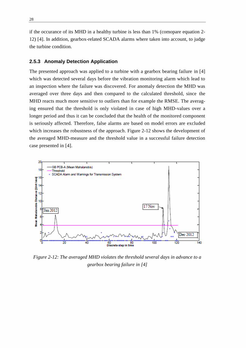
28
if the occurance of its MHD in a healthy turbine is less than 1% (comopare equation 2-
12) [4]. In addition, gearbox-related SCADA alarms where taken into account, to judge
the turbine condition.
2.5.3 Anomaly Detection Application
The presented approach was applied to a turbine with a gearbox bearing failure in [4]
which was detected several days before the vibration monitoring alarm which lead to
an inspection where the failure was discovered. For anomaly detection the MHD was
averaged over three days and then compared to the calculated threshold, since the
MHD reacts much more sensitive to outliers than for example the RMSE. The averag-
ing ensured that the threshold is only violated in case of high MHD-values over a
longer period and thus it can be concluded that the health of the monitored component
is seriously affected. Therefore, false alarms are based on model errors are excluded
which increases the robustness of the approach. Figure 2-12 shows the development of
the averaged MHD-measure and the threshold value in a successful failure detection
case presented in [4].
Figure 2-12: The averaged MHD violates the threshold several days in advance to a
gearbox bearing failure in [4]

29
3 Model Development
Against the presented background this thesis aims to further develop and apply the
anomaly detection methodology introduced in chapter 2.5. Therefore, the following
chapters describe the general model development process followed within this thesis
and explain its subtasks. Within the chapters 4 and 5 the described approach is applied
for CM of WTs.
3.1 Model Development Process
The process of developing an ANN based normal behavior model can be divided into
multiple subtasks which together represent an iterative development process. Before a
first model training the input and output parameters have to be selected according to the
desired application. Moreover, a suitable ANN architecture has to be specified. Lastly, a
data pre-processing approach has to be developed, to enable appropriate model training.
After completing these tasks the model can be trained and the result should be verified
during a testing and validation process, where the model is applied to healthy and faulty
WTs. When developing an ANN, it can be difficult to find the optimal network configu-
ration for a specific application, since the performance depends on all the previously
described factors and processes. Thus, finding a suitable ANN for an engineering appli-
cation is always an iterative process, where the pre-training configurations are varied
until a sufficient result is achieved (compare Figure 3-1) [26]. The following sections
describe the general approaches followed by this thesis in the development of the ANN
based normal behavior models.
Figure 3-1: Schematic flow chart of the iterative model development process

30
3.2 Parameter selection
The selection of appropriate input and output parameters is an essential part of ANN
development. In a first step the target parameter has to be selected. Potential component
failures should manifest themselves in the chosen measurement, to enable failure detec-
tion. This shows the importance of target parameter selection for successful anomaly
detection. In many cases there is only little choice because of the limited availability of
measurements addressing the malfunction. In fact, the applicability of the approach of-
ten depends on the availability of potential target measurements.
The selection of input parameters, on the other hand, is more complex. Relevant input
parameters have to be chosen in a way, so that the model is able to predict the target
parameter under normal operating conditions with sufficient accuracy. This ensures a
detectable deviation between the model output and the actual parameter measurement
during a malfunction in the corresponding component. In contrast to the target parame-
ter selection there usually is a big number of potential input measurements to choose
from. Here, the physical relations between the turbine components which result in cor-
relations between the corresponding parameters play a key role. However, only few
works have considered correlations between parameters of the SCADA system at the
stage of parameter selection [24]. In this thesis a comprehensive study of the correla-
tions between component related parameters has been conducted. Figure 3-2 shows the
correlation coefficients between selected parameters. Data representing almost 10 WT
years has been analyzed and the results have been taken into account when selecting the
model inputs.
Figure 3-2: Correlation matrix between different SCADA-parameters
1 2 3 4 5 6 7 8 9 10 11
WTG19_Generator Bearing Temp. Avg. (1)
WTG19_Generator Phase1 Temp. Avg. (2)
WTG19_Generator RPM Avg. (3)
WTG19_Hydraulic Oil Temp. Avg. (4)
WTG19_Gear Bearing Temp. Avg. (5)
WTG19_Gear Oil Temp. Avg. (6)
WTG19_Nacelle Temp. Avg. (7)
WTG19_Rotor RPM Avg. (9)
WTG19_Ambient Temp. Avg. (9)
WTG19_Ambient WindSpeed Avg. (10)
WTG19_Grid Production Power Avg. (11)
Average Correlation Between SCADA-Parameters
Avera
ge C
orr
ela
tion C
oeff
icie
nt
R
0.1
0.2
0.3
0.4
0.5
0.6
0.7
0.8
0.9
1

31
When choosing the model inputs and outputs, two main objectives were considered.
Firstly, the performance of the normal behavior model was optimized to achieve a suffi-
cient accuracy and secondly, the model has to correctly indicate failures as well as pre-
vent false alarms during the application stage. Both conditions were evaluated in the
validation process described in chapter 3.6.
It has been realized that the choice of input parameters should not be based on statistics
only. Even though an input parameter with a high correlation to the target parameter
will probably result in a performance improvement, it can lead to problems in anomaly
detection. This is especially critical if two parameters show high correlation and similar
behavior in case of a component failure. Due to the high correlation the input parameter
is likely to get highly weighted during model training. Thus the parameter will have a
big influence on the model output and improve the model’s performance significantly,
since it gives a clear indication of target parameter. In case of a failure however, this
results in a ‘correct‘ prediction of the abnormal target parameter behavior, which is then
labels as ‘normal’. Figure 3-3 gives an example of such a case. Hence, the turbine’s
physical system relations have to be taken into account during the selection process to
avoid such model behavior.
Figure 3-3: Example for ‘correct’ prediction of abnormally high bearing temperature
by normal behavior model due to incorrect choice of input parameters
3.3 Model Architecture
As mentioned earlier, there is no established standard method for neural network design
and thus a suitable and stable network has to be found in a trial and error process (com-
pare 2.3.1). After defining the input and output parameters, which in engineering appli-
cations are often defined by the technical problem itself, a network topology has to be
determined [26]. Within this thesis, the model architecture was selected based on find-
40
45
50
55
60
65
70
75
80
Tem
pera
ture
in
°C
Model Validation Gearbox
Measured Temperature
Modelled Temperture

32
ings of related projects. In [4] a NARX network with 20 hidden neurons was success-
fully applied for detection of a gearbox failure (compare 2.5.1). The same configura-
tion was found to be sufficient in [40] where parametric studies were carried out to find
the best model architecture for modelling the power output of a turbine. This is why
this configuration was chosen for both models presented later within this thesis. Table
3-1 sums up the selected ANN topology.
Table 3-1: ANN architecture specification for all developed models
ANN Type NARX
Layer Hidden Output
Neurons 20 1
Activation Function Sigmoid Threshold
3.4 Data Pre-Processing
After successful determination of model architecture and parameters, the network needs
to be trained. To build a functioning normal behavior model, the training data presented
to the ANN has to represent normal operating conditions of the turbine. This is especial-
ly important since the synaptic weights are decided solely based on the training data,
without any physical understanding of the system. If a model has been trained with er-
roneous data, it might not be able to identify abnormal behavior as such and thus fail its
purpose.
Unfortunately, data extracted from SCADA system is usually not ‘clean’. Malfunctions
in the SCADA communication system, sensor or signal processing errors and standstill
during maintenance and repair actions lead to missing and faulty data points, hidden in
the large data sets. Also it cannot be guaranteed, that the complete data set selected for
training does not contain any traces of minor errors during this period. To make sure
that the ANN training is not distorted by such measurements, faulty data is removed
from the training data set by applying an initial data screening and filtering process.
In general, it was realized that SCADA systems form different manufacturers report the
measurements with variable reliability. Some systems reported more than 95 % of the
yearly operational data points correctly, whereas in others only around 50 % of the data
sets were complete. This also depends on the recording philosophy. Some systems keep
recording measurements, when the turbine is out of operation, others do not. However,
sufficient model training was found to be possible also in cases with only half of the
training subsets available, provided that the training data set covers the whole range of
normal operation throughout the application period.

33
Since the data pre-processing is model specific, it is described in the corresponding
model sections (compare chapter 4.1.2 and 5.1.2).
3.5 Model Training
Model training is a crucial factor for the successful application of ANN based normal
behavior models, since the application performance highly relies on the training data
presented to the net. The data pre-processing ensures that unhealthy data is removed
from the training sets. However, it is not guaranteed that the training data covers the full
range of normal operating conditions. This is particularly important because at presence
ANNs are not good at extrapolating information beyond the training domain [26]. On
the other hand, too much training data leads to extensive training times and overfitting,
which again results in a decrease of the models application performance. This is why it
is important to select appropriate training periods.
3.5.1 Training Period and Turbine Individual Networks
For sufficient model training, it is very important, that the training data presented to the
network covers the complete scope of the relevant parameters as well as their combina-
tions and patterns for healthy turbine behavior. For the turbines located in Sweden, dis-
tinctive seasonal variations of operating parameters, especially temperatures, were ob-
served (compare Figure 3-4). Consequently, training data representing the period of a
whole year was used to train the networks, if available. 70 % out of this data is used for
model training, 15 % for testing and 15 % for an initial validation.
Figure 3-4: Turbine specific behavior profile of gear bearing temperatures throughout
a year [4]
Figure 3-4 also explains why it was decided to train one individual model for each tur-
bine instead of developing one general model which can be applied to several turbines.

34
It can be observed that the same parameter, in this case a gear bearing temperature,
shows significantly different behavior from turbine to turbine, even though all of them
are located in the same geographical area and are facing similar environmental condi-
tions. Therefore, individual models can approximate the selected operational parameters
more precisely and thus are better suited for accurate normal behavior modelling. Indi-
vidual turbine behavior can be modelled with the help of ANNs by training the network
with data from a particular turbine, resulting in a unique, turbine specific model.
3.5.2 ANN Training
The LMA, which is used within this thesis to train the ANNs, starts model training with
a random initialization of synaptic weights, which are then optimized (compare chapter
2.3.2). This means that networks which are exposed to the same training data sets get
slightly different synaptic weights assigned during the training process. In general, this
is not a problem, since the differences are marginal, but it is possible that the training
process gets stuck in a local minimum which leads to a relatively bad performing mod-
el. In order to prevent this, n-number of ANNs are trained with the same input data and
the model with the best performance is consecutively chosen. This ensures that the
model, which will later be applied for anomaly detection does not show particularly bad
performance. Within this thesis, the number of trainings to choose the best ANN from
was arbitrarily chosen as three. However, a larger number can be chosen but at cost of
computation time.
3.5.3 Inconsistencies in ANN Training
The random initialization of the synaptic weights at the beginning of the training pro-
cess leads to a unique ANN at the end of each training session. The best-of-three-
trainings practice, described in the previous paragraph, excludes the possibility of an
unusually bad training result. It has been observed that different trainings lead to net-
works which model the target parameter with only small variations, if the application
input is in the range the network has been trained for (compare top chart Figure 3-5).
Nevertheless, the random synaptic weight initialization can cause problems in anomaly
detection stage. In case data is presented to the network it has not seen during training,
which is a plausible scenario in case of a malfunction, since the network has been
trained with healthy turbine data only, the ANNs might have weaknesses in extrapolat-
ing beyond the training domain. That can lead to model responses, which differ signifi-
cantly from training to training in case of a malfunction (compare bottom chart Figure
3-5).

35
Figure 3-5: Bearing temperature measured and modelled with different trainings for
healthy (top) and faulty (bottom) turbine
This behavior can lead to inconsistent results in anomaly detection, since the model’s
response to unknown data can vary. Especially the dates of first alarms ahead to a fail-
ure can vary for different model trainings. Since time of failure detection is an important
criterion for successful CM, a more steady approach was developed, which allows re-
producible results. In the training-process 100 ANNs, instead of one, are trained with
identical data. Later on during the application process, all these 100 ANNs are used for
the anomaly detection and the average MHD of all 100 models is calculated to judge the
component condition. This approach for the model structure is visualized in Figure 3-6.
Figure 3-6: Structure of Model Training and Application
54
56
58
60
62
64
Te
mp
era
ture
[°C
]
Target Temperature
Modelled TemperaturesMultiple Trainings
54
56
58
60
62
64
Te
mp
era
ture
[°C
]

36
Following this methodology, model training becomes a computationally intensive task.
300 network trainings, 100 times the best of three, have to be conducted before the ap-
plication. The approach resulted in training times of several hours for the ANNs applied
in this thesis. Nevertheless, it was decided to be worth the effort, due to the increased
model quality and the fact that this is a nonrecurring process, which has to be performed
only once, before model application.
3.5.4 Lag and Normalization Consideration
Signals in WTs have usually different time constants to respond to certain operational
events. A ramp up of the wind speed, for example, results in an increased power pro-
duction as well as a higher loading of mechanical components, such as bearings and
gears. These increase in loading leads to higher temperatures within these components,
which are detected by the corresponding SCADA-sensors. However, the temperature
rise will follow the production increase with a certain delay; due to the component’s
thermal inertia [25]. When using feed-forward networks to model normal behavior this
has to be taken into account by implementing appropriate time lags between the input
signals. These lags can be identified by analyzing the cross-correlation between the in-
put parameters. This analysis has been conducted for the present models but did not
result in an improvement of the model’s performance. It is concluded, that the recurrent
network used in this study is able to account for delays through the implemented feed-
back loop.
Moreover, [26] points out that normalization of data presented to the network can sig-
nificantly increase the training speed. Therefore, training was conducted with all param-
eters normalized to values between 0 and 1 using equation 3-1:
(3-1)
With parameter normalization indeed higher training speeds were achieved. However,
due to the decrease in performance the ANN is trained and applied to absolute values.
3.6 Model Evaluation and Validation
Within the iterative development process the model is tested and evaluated after each
ANN training to judge the effects of the previously conducted adjustments. During
training, the model errors have been minimized for the training data set and the outputs
are usually close to the measured values of the target parameter. However, the net-
work’s generalization abilities have to be tested by applying it to data never seen before
[26]. Therefore, each model is applied to a healthy turbine data set to assess the model
performance under normal operating conditions. Furthermore, it is also applied to a
faulty turbine data set, to test the failure detection ability. Only if both validations where

37
conducted with sufficient results, the model is applied to study cases with this configu-
ration.
3.6.1 Training Evaluation
The training data set itself is divided into three subsets. 70 % of the data was used for
actual model training, meaning optimizing the synaptic weights of the ANN. The se-
cond subset, representing 15 % of the training data, is called validation subset. Its error
is monitored during the training process and once the performance decreases the model
training is stopped. The remaining 15 % of the data is the so called test data set. Since
the ANN hasn’t seen this data during training, it can be used to judge the networks gen-
eralization abilities [29].
During ANN training a problem called overfitting can occur. The network memorizes
the training examples and the training error is driven to a very small value. However,
the ANN is not able to generalize well which leads to bad performance in case it is pre-
sented to new data. If the test error increases significantly before the validation error
during training, overfitting might have occurred. Therefore, the errors are monitored to
ensure that no overfitting occurs [29].
Also, the training errors and their distribution have been analyzed. In case a model fits
the data correctly, a random and therefore normal distribution of the model errors can be
observed. Hence, it can be concluded that the model fits the data well if the errors are
normally distributed [38]. Therefore, histograms of the training errors are plotted and
evaluated.
3.6.2 Healthy Turbine Application
There are two main reasons for applying the trained model to a completely healthy tur-
bine. The first one is to test its generalization abilities, when it is exposed to data it has
not seen before and the second one is, to ensure that the anomaly detection approach
does not cause false alarms.
The trained model is applied to a healthy turbine for a full year, consecutive to the train-
ing period. Filtering processes are conducted for training as well as the application data
to ensure failure free data sets. Afterwards the trained ANN is applied to the unseen
data set, which consists of only healthy data. Several conclusions can be drawn from the
results. Firstly, the model performance is evaluated by calculating the MSE and the
RME over a full year of application. The errors give an indication of how precise the
model is able to predict the target parameter. The relative changes of errors were used to
evaluate the impact of a model modification.

38
Secondly, the model is tuned to avoid false alarms. Therefore, the anomaly detection
approach is applied to the healthy turbine (compare 2.5.3). The MHD-measure is sensi-
tive to outliers and is therefore well suited for their detection. However, it is desired to
prevent false alarms caused by inaccurate model prediction instead of a component
fault. This is why the MHD-measure is averaged over a certain time period, which will
damp the absolute MHD value in case the high MHD measure was caused by inaccurate
modelling. However, if the high MHD-value was caused by a component malfunction
the MHD will show high values over the whole period and thus indicate a failure de-
spite the averaging. The model presented in [4] averaged the MHD over a period of
three days (compare 2.5.3). Since the models presented in this thesis predict the target
parameter with a higher accuracy, an averaging period of only one day has been found
to be sufficient. This higher resolution provides comparable model robustness but al-
lows earlier alarms compared to the three day average. Moreover, it was decided to ne-
glect days where there is, in total, less than 6 hours of measurements available, since
this was considered to be insufficient information to judge the turbine condition.
3.6.3 Faulty Turbine Application
It has to be noted, that it is not always the most accurate model which delivers the best
results for anomaly detection. A model with a great performance and causing no false
alarms is worth nothing if it cannot detect component failures as desired. That’s why the
model application to a faulty WT data during validation is the most sensitive part. Pro-
vided the model was successfully validated with the healthy turbine, it can be used for
failure detection in case the failure is detected ahead of its occurrence.

39
4 Gearbox Model
As shown in chapter 2, gearboxes are among turbine’s most critical components in
terms of reliability. Therefore, successful gearbox condition monitoring can be benefi-
cial for turbine operators. The existing model presented in chapter 2.5.1 was able to
predict a gearbox bearing failure in advance. However, this model was not directly ap-
plicable to the turbines of Stena Renewables because input parameters are required,
which were not available in their SCADA-data system. Thus the current model was
modified and further developed accordingly. Its development and the application are
presented in the following sections.
4.1 Model Development and Training
In the previous chapter (compare chapter 3) the general model development process,
which is followed in the development of all subsequently presented models, was intro-
duced. In order to correctly interpret the results of the case studies presented later on, it
is necessary to specify the individual model configurations, which is the subject of the
following subchapters. Firstly, the selected input and target parameters will be dis-
cussed. Then, the conducted data processing will be described in detail. Finally, after
presenting its validation results, the developed gearbox model will be applied to differ-
ent study cases in chapter 4.3.
4.1.1 Parameter Selection
The selection of input and output parameters plays a crucial role in the development of
the ANN as well as the anomaly detection approach. As a first step the available
SCADA-data sets where screened to get an overview of the available parameters. It was
realized that not all parameters used in the presented gearbox model (compare chapter
2.5) were available and thus a new input/output selection process had to be conducted.
Here, the correlations between the parameters as well as their technical relations were
taken into account (compare chapter 3.2). The aim of the iterative selection process was
to achieve high model accuracy in combination with the models capability to success-
fully detect gearbox failures. These requirements lead to the final parameter configura-
tion, which can be seen in Figure 4-1. Moreover, the following subsections describe the
development process in detail.

40
Figure 4-1: Visualization of final gearbox model parameter configuration with inputs
(blue) and targets (violet)
Target Parameters
When monitoring the condition of a gearbox, it is an effective way to monitor its bear-
ings since the majority of gearbox failures actually come along bearing problems [8].
Even if the failure is not caused by the bearing itself, malfunctions in other gearbox
components often manifest themselves as bearing damages and thus can be detected
indirectly [9].
The gear oil acts as lubricant and cooling medium for gears and bearings. This means
that malfunctions which are causing an increased friction between the gear wheels or
the bearings will affect the gear oil temperature. Thus, selecting this parameter as a tar-
get is well suited for gearbox condition monitoring. This is why the gear oil temperature
is typically recorded and automatically compared to a preset threshold within the
SCADA alarm system. The advanced monitoring method developed within this thesis
aims to expand the potential of this approach.
The SCADA data sets of the WTs owned and operated by Stena Renewables contain
two gearbox related parameters and both were selected as input parameters: The tem-
perature of the high speed shaft bearing and the gear oil temperature each averaged over
10 minute intervals with a resolution of 1 °C steps.
Input Parameters
The study on which parameters mainly influence the selected target parameters has re-
vealed that high power output and rpm are likely to come with high bearing tempera-

41
tures. Figure 4-2 visualizes this relationship. Analogue behavior can be observed for the
gear oil temperature.
Figure 4-2: Gear bearing temperature depending on power output and rotor rpm
The correlation analysis shows that there is indeed a high correlation between rotor rpm
as well as power production and the target temperatures (compare Figure 4-3). The rotor
rpm correlation, averaged over more than 10 turbine years, was higher than 0.8 for both
target parameters and higher than 0.75 for the power output. Considering this fact, it
was concluded that these are good indicators for the mechanical loading of the gearbox.
For that reason they were selected as input parameters for both models.
Figure 4-3: Gearbox related parameter correlations averaged over more than 10
healthy turbine years

42
Figure 4-3 also shows that both target parameters are highly correlated. This suggests
that using one as an input to model the other might improve the models quality, since
the gear oil temperature gives a clear indication of the bearing temperature and vice
versa. A parameter study, where different input configurations were investigated con-
firmed that. Figure 4-4 shows the relative performance of the gear bearing model aver-
aged over 20 model trainings for different input configurations.
Figure 4-4: Relative performance gear bearing model based on the MSE for different
model input configurations and indication of the model’s anomaly detection ability.
However, it is not necessarily the most accurate model that is best suited for failure de-
tection, as Figure 4-4 shows. Even though the configuration including both gear-related
parameters shows by far the best performance, it is not able to detect a gearbox failure.
Through their high correlation the parameters are getting highly weighted during model
training and therefore strongly influence the model output. In case of a failure both tem-
peratures increase resulting in a 'correct' prediction of the abnormally high target tem-
perature. Due to this behavior, the parameters cannot be used as inputs for one and an-
other.
For the selection of the remaining input parameters the physical system behind the sta-
tistical numbers was taken into account. Nacelle and ambient temperature correlate only
little with the target parameters (compare Figure 4-3), which might lead to the conclu-
sion that they are not important for successful model application. Indeed, they seem not
to contribute very much to the model’s accuracy but anyway they are of big importance
for anomaly detection. Successful failure detection was possible only if both tempera-
tures were used as model inputs (compare Figure 4-4). The reason is that all four tem-

43
peratures, gear bearing, gear oil, nacelle and ambient temperature are coupled via heat
exchangers and cooling fans. In addition, nacelle and ambient temperature are highly
correlated (compare Figure 4-3). Therefore, a failure, which results in an increased fric-
tion within the gearbox, does not necessarily cause extreme temperatures within the
gearbox. The cooling mechanisms can keep the temperatures in the regular range, but
this will then disturb the normal association between nacelle and ambient temperature.
It was found to be essential to include both measurements as inputs into the model.
Since the gear bearing and the gear oil temperature are closely related, the respective
analysis for the gear oil model showed qualitatively identical results. Thus, the input
configuration marked in Figure 4-4 was chosen for both models.
4.1.2 Data Pre-Processing
After parameter selection the data pre-processing is net next step to discuss. Several
filter methods have been developed for the gearbox model to remove erroneous data
form the training set and prevent false alarms due to signal errors during application
stage. During the filtering process approximately 20-25 % of the data points are deleted
from the selected training data set. Most of the data loss is normally caused by the gen-
eral boundary filter (GBF). The GBF is responsible for removing abnormally high and
low values caused by communication errors as well the data sets recorded during tur-
bine standstill, when the turbine is not in operation. Table 4-1 gives an overview of the
filters and their application.
Table 4-1: Overview of filters of the gearbox model
Filter Purpose Data
Losses
Application
TR Set APP Set
General Missing Filter Filter missing values ~ 1-5 % x x
General Boundary Filter Filter high/low values
and standstill data ~ 10-20 % x x
General Cluster Filter Removes abnormal data
from training set 2.5 % x -
Skip Filter Filter values after missing ~ 1-2 % x x
Figure 2-1 visualizes their impact on the training data set. Looking at Figure 2-1 it has
to be noted that the skip filter does not cause a gap in the low range of the power curve.
This is just a visual impression since the filter data points were added to the plot after
the remaining data point and thus partially cover them. In the following paragraphs the
purpose, conditions and results of the individual filters are explained in detail.

44
Figure 4-5: Visualization of the different filters applied within the gearbox model
General Missing Filter
Since the model cannot be either trained or applied with incomplete data sets, the data
points had to be neglected whenever one of the parameters used by the model was miss-
ing. Therefore, the general missing filter screens the subsets consisting of all relevant
input and target parameters of all time steps for missing values and deletes the
whole subset from the training or application data set if one of the parameters is not
recorded (compare equation 4-1).
(4-1)
General Boundary Filter
SCADA communication problems and sensor malfunctions can lead to unreasonable
values reported by the SCADA system. The GBF aims to exclude these values from the
training data set as well as from the application data set, since wrongly reported parame-
ters should not lead to an alarm of the normal behavior model. Therefore, the relevant
parameters are filtered in case they exceed the operational boundaries specified in the
manufacturer’s technical documentation (compare equation 4-2).
(4-2)
Furthermore, the filtering of data subsets with a turbine production below zero guaran-
tees that only data sets which represent the turbine during operation are taken into ac-
count. The GBF typically excludes around 10 to 20 % of the initial data values, most of
them based on the power filtering. The boundaries applied within this thesis are pre-
sented in in Table 4-2 and Figure 4-6 visualizes its application to a data set. It can be
seen that mainly data points with a negative production are filtered.

45
Table 4-2: GBF-boundaries for parameters of the gearbox model
Gearbox Parameters Rated Value
Lower Bound
Upper Bound
Grid Production Power Avg. [kW] 2000 0 2000
Rotor RPM Avg. [rpm] 16.7 0 17
Gear Bearing Temp. Avg. [°C] - -20 90
Gear Oil Temp. Avg. [°C] - -20 80
Nacelle Temp. Avg. [°C] - -20 70
Ambient Temp. Avg. [°C] - -20 40
Figure 4-6: Visualization of the General Boundary Filter
General Cluster Filter
The training data sets for the normal behavior models consist of large spreadsheets con-
taining operational data records of multiple months. Even though there was no failure
documented for a specific turbine, it cannot be excluded that minor malfunctions have
left their traces in the SCADA data. Since these data points do not represent normal
behavior, they should be excluded from the training data. Removing these outliers from
the training set can improve a model significantly, if the data is not characteristic for the
problem domain [26]. Therefore, a filtering method introduced in [40] was applied in
this thesis. There, outliers in the training data set are found and filtered by clustering the
input data and using the MHD to define outliers.
Firstly, every training data subset is assigned to one of the clusters based on its average
wind speed, ambient temperature and pitch angle (compare Table 4-3). This is conduct-
ed using MATLAB’s clusterdata function, which bundles data points based on their

46
relative Euclidean distance. Afterwards the multidimensional MHD of each subset from
the cluster center is calculated (compare 2.4.3). The eight parameters taken into account
can be found in Table 4-3 and Figure 4-7 visualizes the effect of the cluster based filter-
ing.
Table 4-3: Specification of parameters for clustering of data set and parameters used
for filtering with MHD
Cluster Parameters Filtering Parameters
Power output avg./std.
Wind speed avg. Wind speed avg./std.
Ambient temperature avg. Pitch angle avg./std.
Pitch angle avg. Rotor RPM avg.
Ambient temperature avg.
Figure 4-7: Visualization of the General Cluster Filter
In some of the data sets the pitch angle information was incomplete. In that case these
values were not taken into account in the filtering approach and the number of clusters
was reduced to 12 following the logic of [40]. Sufficient filtering results were achieved.
Finally, the distances of all data points from their cluster centers are compared and the
subsets which show the top 2.5 % MHDs are considered to be outliers and are conse-
quently removed from the data set. The condition for deleting a subset is presented
in equation 4-3, where MHDxt represents the MHD of the subset from the cluster center

47
and CDFMHDxt the clusters cumulative distribution function of the MHDs, assuming a
log logistic distribution.
(4-3)
With the help of this method abnormal data points hidden in the large training data set
can effectively be identified and removed which leads to an improvement of model per-
formance.
Skip Filter
When evaluating the ANN’s abilities to model the target temperatures, it has been ob-
served that comparably big prediction errors occurred after periods where data is miss-
ing for a longer time. These data gaps can be caused either by turbine downtimes or by
data filtering. However, during the first few measurements after these periods the model
usually overestimated the target temperatures (compare Figure 4-8) resulting in false
alarms during the application stage.
Figure 4-8: Temperature overestimation after large data gaps
The explanation for this phenomenon is based on the fact that all data is presented to the
ANN as continuous measurements and the ANN has no indicator for the data interrup-
tions. During the times where data is missing, the turbine is most likely out of operation
and the gearbox substructures cool down over time. The turbine power output and RPM
as input parameters are the model’s only indicators for the gearbox loading. In case pro-
duction ramps up, the consequent temperature increase in gearbox components will fol-
low with a delay, due to the thermal inertia of the gearbox subsystems. This has two
negative effects on the model. Since the training algorithm tries to fit the training targets
Q1-14 Q2-14 Q3-14 Q4-140
0.5
1
1.5
2
2.5
3
3.5
4
Date
Ma
ha
lan
ob
is D
ista
nc
e
Gear Oil Model
Average Mahalanobis Distance
Normal Operation Limit
SCADA Alarms/Warnings
Data Missing

48
as good as possible, the combination of these low temperatures and high loading indica-
tors lead to a performance decrease in form of a slight temperature underestimation dur-
ing regular operation. Moreover, the model is still not able to predict the low tempera-
tures after turbine standstill and thus it overestimates the temperatures after these inac-
tive periods.
As a solution to this problem a dual approach has been followed. On one hand, the TSF
has been developed, which excludes the after downtime data from training and applica-
tion process. This results in a better performing ANN and prevents false alarms during
application stage. The filter was tuned due to analysis of the model output, which re-
vealed that the ANN had difficulties to model the target temperatures correctly mainly
during the hour following a long downtime (see Figure 4-8). Afterwards the tempera-
tures reached the normal operation range again and the model error returned to a tolera-
ble level. Moreover, it was decided to apply the filter only in case there was not a single
measurement for a period of at least three consecutive hours. Figure 4-9 visualizes the
effect of the TSF. The application resulted in a significant overall performance increase
(compare Figure 4-10).
Figure 4-9: Visualization of the Skip Filter
On the other hand, an indicator for discontinuous input data has been introduced and the
performance of the ANN model has been optimized in an iterative study. The general
idea is to introduce an additional input signal to the ANN model. This value of the input
signal is dependent on the length of missing data before the current data point. This is
conducted for both the training and the application data set. For the optimization differ-
ent configurations were run for ten times each and the performance was documented
(compare Figure 4-10).

49
Figure 4-10: Performance for different configurations for the skip filter and parameter
The best average and most consistent performance were achieved with the following
skip parameter configuration. The parameter was chosen to be:
zero, if there is no gap and the previous data point is available
one, if only the previous data point is missing which corresponds to a gap of 10
minutes
two in case that previous to the data point there was a gap of at least three con-
secutive hours without an available measurement
The output analysis as well as the skip parameter optimization came to qualitatively
identical results for both target parameters. This is why the both methods are applied
with the same configuration to the gear bearing temperature as well as the gear oil tem-
perature model.
4.2 Validation and Comparison
Healthy Turbine
For model development and verification the model with its presented configurations
was applied to one year of operational data from a turbine without any reported failures.
Figure 4-11 shows the model output in comparison to the measured values for a period
of three days. It can be observed that both models are able to predict the temperatures
accurately.

50
Figure 4-11: Measured versus modelled temperatures for a healthy turbine
The ANNs were able to model the gear bearing temperature with an average MSE/MAE
of 0.732/0.556 and the gear oil temperature with an average MSE/MAE of 0.956/0.580,
all measures in °C. Thus, a higher model accuracy was achieved than in comparable
studies, where bearing temperatures in WTs where modelled using ANNs (compare
Table 4-4). The reasons for the increased accuracy lay mainly the data pre-processing
and the data quality.
Table 4-4: Model performance for healthy turbine application averaged over 20 ANNs
in comparison with literature values.
Model Description MAE MSE Source
Gear Bearing Model Thesis
model with presented con-figuration
0.56 0.73 -
Gear Oil Model Thesis
model with presented con-figuration
0.58 0.99 -
Gear Bearing Model Zaher
ANN based gear bearing temperature modelling
- 1.51* [21]
Gear Oil Model Zaher
ANN based gear oil tempera-ture modelling
- 4.88* [21]
Generator Bearing Kusiak
ANN based generator bear-ing temperature modelling
0.69 - [32]
03/04/14-00:00 12:00 03/05-00:00 12:00 03/06-00:00 12:00 03/07-00:0035
40
45
50
55
60
65
Date
Te
mp
era
ture
in
°C
Gear Bearing Model
Measured Temperature
Modelled Temperture
03/04/14-00:00 12:00 03/05-00:00 12:00 03/06-00:00 12:00 03/07-00:0035
40
45
50
55
60
65
Date
Te
mp
era
ture
in
°C
Gear Oil Model
Measured Temperature
Modelled Temperture
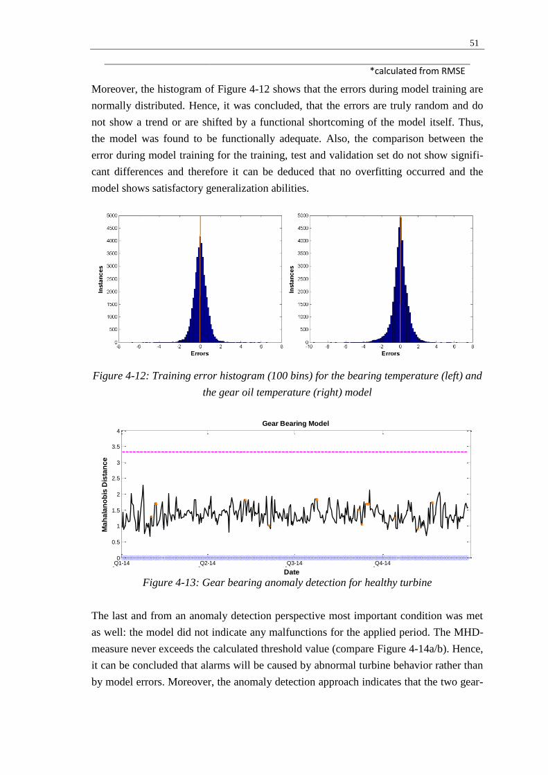
51
*calculated from RMSE
Moreover, the histogram of Figure 4-12 shows that the errors during model training are
normally distributed. Hence, it was concluded, that the errors are truly random and do
not show a trend or are shifted by a functional shortcoming of the model itself. Thus,
the model was found to be functionally adequate. Also, the comparison between the
error during model training for the training, test and validation set do not show signifi-
cant differences and therefore it can be deduced that no overfitting occurred and the
model shows satisfactory generalization abilities.
Figure 4-12: Training error histogram (100 bins) for the bearing temperature (left) and
the gear oil temperature (right) model
Figure 4-13: Gear bearing anomaly detection for healthy turbine
The last and from an anomaly detection perspective most important condition was met
as well: the model did not indicate any malfunctions for the applied period. The MHD-
measure never exceeds the calculated threshold value (compare Figure 4-14a/b). Hence,
it can be concluded that alarms will be caused by abnormal turbine behavior rather than
by model errors. Moreover, the anomaly detection approach indicates that the two gear-
Q1-14 Q2-14 Q3-14 Q4-140
0.5
1
1.5
2
2.5
3
3.5
4
Date
Ma
ha
lan
ob
is D
ista
nc
e
Gear Bearing Model
Q1-14 Q2-14 Q3-14 Q4-140
0.5
1
1.5
2
2.5
3
3.5
4
Date
Ma
ha
lan
ob
is D
ista
nc
e
Gear Oil Model
Average Mahalanobis Distance
Normal Operation Limit
SCADA Alarms/Warnings
Data Missing

52
related SCADA alarms do not reflect serious gearbox damages, since there is no model
alarm.
Figure 4-14b: Gear oil anomaly detection for healthy turbine
Faulty Turbine
Furthermore, the model was applied to a turbine with reported gearbox problems to val-
idate the anomaly detection abilities. Therefore, the turbine which is presented as study
case in [4] was selected since the cause of failure events is well documented and under-
stood. In this particular turbine a failure in the low speed shaft occurred. Temperature
measurements for the damaged bearing, the high speed shaft bearing and the gear oil are
available. With a slightly less aggressive filtering approach due to low data availability
around the failure the results listed in Table 4-6 were achieved.
Table 4-5: Results of anomaly detection for LSS-bearing failure
LSS-Bearing Model
Vibration CM-system
Inspection HSS-Bearing Model
Gear Oil Model
Alarm 17. Nov.
Alarm 23. Nov.
Discovery 28. Nov.
No Alarm No Alarm
The results confirm the model’s ability to detect failures in advance. The alarm was
issued the same day the model in [4] detected the failure. Moreover, the importance of
measurements from the damaged component itself can be seen. The models for HSS
Bearing and Gear oil did not indicate an error, which enables one to localize the prob-
lem in the gear box. However, all three models detected the final breakdown of the
gearbox.
Q1-14 Q2-14 Q3-14 Q4-140
0.5
1
1.5
2
2.5
3
3.5
4
Date
Ma
ha
lan
ob
is D
ista
nc
e
Gear Oil Model
Average Mahalanobis Distance
Normal Operation Limit
SCADA Alarms/Warnings
Data Missing

53
4.3 Model Application
This section presents the application of the proposed ANN model to data of turbines
operated by Stena Renewables. For the selected turbines gearbox problems were rec-
orded and thus they are well suited to investigate the model’s failure detection ability.
Table 4-6 summarizes the model configuration and training specifications used for the
anomaly detection.
Table 4-6: Summary of gearbox model specifications
NARX ANN Configuration
Layer Hidden Output
Activation Function Sigmoid Threshold
Neurons 20 1
Inputs Power
Rotor RPM Nacelle Temperature
Ambient Temperature
Outputs Gear HSS Bearing & Gear Oil Temperature
Training and Data Pre-processing
Training Algorithm Levenberg-Marquard
Training Period 1 failure free year of data
Filter Training Data Boundary Filter Cluster Filter
Skip Filter
Training Philosophy 100x best of 3 trainings
Application and Anomaly Detection
MHD Averaging Over one day
Data Sufficiency Limit At least 6h of data over one day
4.3.1 Gearbox Study Case 1
Case Description
In this particular turbine, which was commissioned in 2008, an IMS-bearing failure
resulted in a complete gearbox failure and the gearbox had to be replaced consequently.
The bearing failure was first discovered during an inspection which was conducted due
to an alarm of the vibration system on the 25th
of April 2014. A crack on the inner ring
of the IMS-bearing was discovered. Also, beginning of spalling was reported and a
bearing replacement was recommended. However, it was decided to further operate the
turbine, since long lead times would have caused production losses. The turbine was
operated for more than one more month with the damaged bearing until the complete
gearbox failed. Turbine operation was stopped on the 22nd
of May and the gearbox re-
placement was conducted from the 3rd
of June on.

54
Anomaly Detection
In Figure 4-15 the measured temperature values versus the ANN output for the gear
bearing and the gear oil are presented for the period previous to the failures. The meas-
ured temperature does not show abnormally high values until its steep increase immedi-
ately before the complete gearbox failure. It can be observed that both models are able
to predict the development of the temperatures quite accurately with two exceptions
(marked in Figure 4-15). Around the 20th
of March both models over-predict the tem-
peratures for a short period and the extremely high temperatures shortly before the
gearbox failure are not modelled correctly. The temperatures deviations suggest that
there are periods where the turbine is not operating normally.
Figure 4-15: Modelled and measured temperatures before gearbox failure
Figure 4-16 shows the MHD-measures versus the calculated threshold in the months
ahead of the gearbox failure. It can be observed that both models trigger an alarm on the
20th
March due to the overvaluation. Around the period where the IMS-problems are
documented neither the bearing model nor the oil model triggers an alarm. The period
of the inspection can be identified due to the missing data at the end of April. The final
model alarm occurred on the 22nd
of May, the day when the turbine was taken out of
operation. A closer look into the modelled versus the measured temperatures show, that
Mar Apr May30
40
50
60
70
80
Date
Te
mp
era
ture
in
°C
Gear Oil Model
Measured Temperature
Modelled Temperture
Mar Apr May30
40
50
60
70
80
Date
Te
mp
era
ture
in
°C
Gear Bearing Model

55
there is a sudden increase of both measured temperatures causing a significant deviation
between the modeled and measured parameters, which manifest themselves as high
MHD-values. That day also multiple gearbox-related SCADA-alarms were triggered,
which was probably the reason for the turbine shutdown.
Figure 4-16: Anomaly detection of both models before gearbox failure
Initial Alarm Analysis
The anomaly detection plots (Figure 4-16) show a clear violation of the threshold at the
end of March. As sudden as the increase occurs on the 20th
of March it decreases again
only one day later and the following period does not show any anomalies till the IMS-
bearing was discovered. To find the explanation of the high MHD value, a closer look
on the modelled versus the measured gear bearing and gear oil temperatures is helpful.
Figure 4-17 shows that both models overestimate the target values noticeably which
causes the threshold violation.
Mar Apr May0
2
4
6
8
10
12
Date
Ma
ha
lan
ob
is D
ista
nc
e
Gear Bearing Model
Average Mahalanobis Distance
Normal Operation Limit
SCADA Alarms/Warnings
Data Missing
Initial alarm
IMS-bearing inspection
Complete gearbox failure
Mar Apr May0
2
4
6
8
10
12
Date
Ma
ha
lan
ob
is D
ista
nc
e
Gear Oil Model
Initial alarm
IMS-bearing inspection
Complete gearbox failure
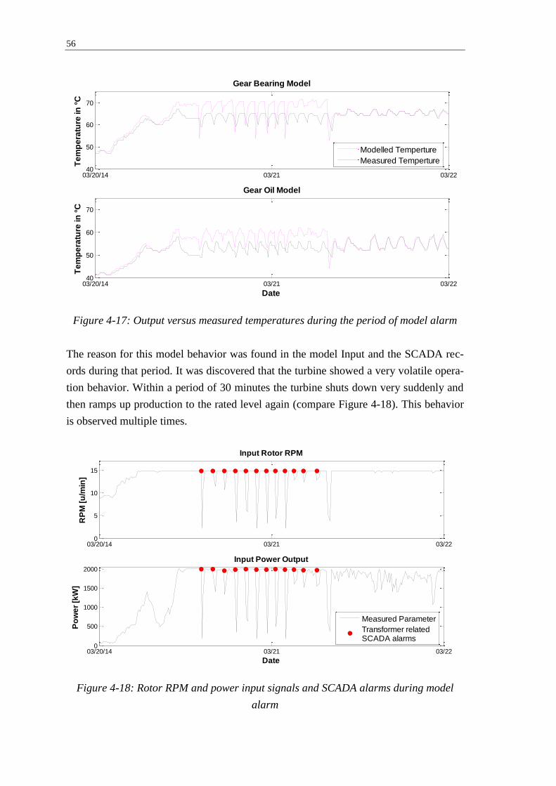
56
Figure 4-17: Output versus measured temperatures during the period of model alarm
The reason for this model behavior was found in the model Input and the SCADA rec-
ords during that period. It was discovered that the turbine showed a very volatile opera-
tion behavior. Within a period of 30 minutes the turbine shuts down very suddenly and
then ramps up production to the rated level again (compare Figure 4-18). This behavior
is observed multiple times.
Figure 4-18: Rotor RPM and power input signals and SCADA alarms during model
alarm
03/20/14 03/21 03/2240
50
60
70
Gear Bearing ModelT
em
pe
ratu
re in
°C
03/20/14 03/21 03/2240
50
60
70
Gear Oil Model
Date
Te
mp
era
ture
in
°C
Modelled Temperture
Measured Temperture
03/20/14 03/21 03/220
5
10
15
Input Rotor RPM
RP
M [
u/m
in]
03/20/14 03/21 03/220
500
1000
1500
2000
Input Power Output
Po
we
r [k
W]
Date
Measured Parameter
Transformer relatedSCADA alarms

57
A look into the SCADA records revealed that there were more than ten alarms caused
by very high temperatures in the converter, which lead to the automatic turbine shut-
downs. After a few minutes, when the temperatures returned to an acceptable level, tur-
bine operation was started again until the high temperatures occurred again. This behav-
ior was repeated every two hours until the operation was manually stopped by the oper-
ator. The models are not able to model predict their target parameters accurately under
these circumstances, since the models weren’t trained for these abnormal input signal
behavior.
Therefore, it was concluded that the initial alarm was not related to the later failure of
the IMS-bearing, even though it cannot be excluded that the volatile behavior contribut-
ed to the bearing degradation. Taking the absence of gear-related SCADA-alarms and
the transformer alarms into account, the operator can conclude that the alarm of the
gearbox model was not connected to the gearbox itself. In fact, the model might draw an
operator’s attention to the turbine and the manual operation stop with an inspection
could have been conducted earlier.
Summary and Conclusion
Table 4-7 summarizes the failure description and the model’s anomaly detection results:
Table 4-7: Summary of gearbox study case 1
Inspection Reports SC01
Date Source Description
25.04.2014 Vibration-System CMS-alarm
25.04.2014 Inspection IMS-bearing damage discovered
22.05.2014 SCADA alarm Turbine operation stopped
03.06.2014 Maintenance Gearbox replacement
Anomaly Detection SC01
20.03.2014 Bearing Model Alarm caused by abnormal operation
20.03.2014 Oil Model Alarm caused by abnormal operation
22.05.2014 SCADA Alarm caused by high temperatures
22.05.2014 Bearing Model Alarm caused by high temperatures
22.05.2014 Oil Model Alarm caused by high temperatures
In the presented study case the gearbox model issued an alarm due to abnormal turbine
operation and finally before the complete breakdown of the gearbox. The IMS-bearing
malfunction itself was not detected. It is concluded, that the bearing problems didn’t
affect any of the monitored variables significantly enough to allow detection. However,
the model was able to detect the severe damage of the gearbox that resulted from the
IMS-bearing failure and gives an additional indicator to pay increased attention to the
multiple SCADA-alarms that were triggered that day.

58
4.3.2 Gearbox Study Case 2
Case Description
The turbine of this study case was installed in November 2006. After 5 years of opera-
tion, from the 19th
November 2011 on, the turbine was standing still although high wind
speeds were measured on site. An inspection two days later revealed that the whole
gearbox was completely stuck and the gearbox was completely broken. The gear oil,
which was changed only 8 days before, showed severe signs of degradation. The gear
wheels were damaged, the rear IMS bearing crashed and debris with tooth-pieces was
found in the gearbox. The complete gearbox had to be changed in consequence.
Anomaly Detection
The measured temperatures of the gear bearing and the gear oil show similar behavior
like in the previous study case. Exceptionally high temperatures occur only right before
the complete gearbox breakdown. However, the comparison with the output of the nor-
mal behavior models shows a difference. The model output starts deviating from the
measurements from the mid of September on (compare Figure 4-19). Both models esti-
mate the temperatures lower than measured. The difference can be observed more clear-
ly for the gear oil model than for the gear bearing model. In addition, the very high tem-
peratures in the last two days are not modelled as normal behavior by the ANNs.
Figure 4-19: Modelled and measured temperatures before gearbox failure
The anomaly detection methodology helps to judge these deviations. A constantly in-
creasing MHD measure can be observed for both models, caused by an increasing devi-
Jul Aug Sep Oct Nov30
40
50
60
70
80
Te
mp
era
ture
in
°C
Gear Bearing Model
Jul Aug Sep Oct Nov30
40
50
60
70
80
Date
Te
mp
era
ture
in
°C
Gear Oil Model
Measured Temperature
Modelled Temperture

59
ation between normal behavior model output and measurement. This development indi-
cates a malfunction with a gradually increasing influence on the gearbox-system. This
development peaks in threshold violations in both models. The gear oil model shows the
first threshold violation on the 13th
of September and the gear bearing model on the 05th
of October. From October on the MHD measure lay above the threshold for most of the
days in both models. Even though there is no gear-related SCADA-alarm, such model
results should be taken serious and a detailed inspection should be initiated. Two days
ahead of the failures the first SCADA-alarms occur together with extremely high MHD-
measures indicating the near complete breakdown of the gearbox. However, the reasons
for the deviation between the ANN output and the temperature measurement have to be
analyzed before a final conclusion can be derived from the results.
Figure 4-20: Anomaly detection of both models before gearbox failure in SC02
Anomaly Detection Analysis
One potential source for ANN errors is an insufficient range of the training data. Then
the ANN would not be able to predict accurately for input data exceeding the range for
which it was trained. Such a situation would result in increased errors in the model and
subsequently a false alarm. It is important to exclude the possibility that the temperature
under estimation presented in Figure 4-18 is not due to short comings in the ANN mod-
el. Therefore, the input signals provided to the ANN model at application stage are
compared to the range of input signals provided during training. In Figure 4-21 all four
input signals are plotted against their training minimums and maximums.
Jul Aug Sep Oct Nov0
5
10
15
Gear Bearing Model
Ma
ha
lan
ob
is D
ista
nc
e
Jul Aug Sep Oct Nov0
5
10
Date
Ma
ha
lan
ob
is D
ista
nc
e
Gear Oil Model
Average Mahalanobis Distance
Normal Operation Limit
SCADA Alarms/Warnings
Data Missing
Gearbox breakdown 19. Nov.
Gearbox breakdown 19. Nov.
First alarm - 13. Sept.
First alarm - 05. Okt.

60
Figure 4-21: ANN input signals and their extreme values in the training data set for the
period when the model triggered alarms
It can be observed, that only the rotor RPM reaches values below its training minimum,
but only for a few instances and in times when the model was actually not triggering
alarms. Therefrom it is concluded that the training data covered a sufficient range.
Moreover, no strange operation behavior, as for example observed in gearbox study
case 1, occurred during the condition monitoring period. It is concluded that the model
alarms are indeed triggered by a malfunction in the gearbox, which lead to a system
imbalance which the model detected successfully. It is assumed that the gearbox mal-
function resulted in an increased friction and heat production in the gearbox. An in-
creased activity of the cooling system would have been able to keep the temperatures
within the gearbox in an acceptable range but has potentially disturbed the relation be-
tween the highly correlated nacelle and ambient temperature, since the failure was only
detectable in case both parameters were selected as ANN inputs.
Summary and Conclusion
In gearbox study case two a successful application of the developed gearbox-model was
demonstrated. This information is especially valuable, since the turbine was equipped
with a vibration CM system which was not able to detect the malfunction at all. Also,
10. Sep/11 Oct Nov 19.Nov10
20
30
40
Te
mp
era
ture
[°C
]
Input Nacelle Temperature
10. Sep/11 Oct Nov 19. Nov0
10
RP
M [
u/m
in]
Input Rotor RPM
10. Sep/11 Oct Nov 19. Nov-20
0
20
Te
mp
era
ture
[°C
]
Input Ambient Temperature
10. Sep/11 Oct Nov 19. Nov0
1000
2000
Date
Po
we
r [k
W]
Input Power Output

61
the SCADA alarms were triggered only two days before the breakdown, due to the ex-
treme temperatures which occurred in the gearbox by that time. The model triggered the
first alarm more than two months before the final gearbox collapsed, sending early sig-
nals of a malfunction. A detailed inspection at that time could have limited the failure
propagation which resulted in the final gearbox breakdown. Table 4-7 summarizes the
failure description and the model’s anomaly detection results:
Table 4-8: Summary of gearbox study case two
Inspection Reports SC02
Date Source Description
19.11.2014 Turbine stuck Turbine operation stopped
22.11.2014 Inspection Gearbox replacement necessary
Anomaly Detection SC02
13.09.2014 Oil Model First malfunction alarm
05.10.2014 Bearing Model First malfunction alarm
17.11.2014 SCADA Alarms caused by high temperatures
4.4 Discussion
The development and application of an ANN based normal behavior model for gear box
condition monitoring was presented in this chapter. In addition to the reported infor-
mation, the discussion of experiences, challenges and future work will conclude this
chapter.
The presented ANNs showed good performance when modelling the target parameters.
This was achieved by selecting appropriate model input parameters, suitable training
configuration, quality of the provided data and last but not least the developed data pre-
processing methods. The data processing can be a work intensive task, but contributes
significantly to the models accuracy by identifying the data points which the ANN has
problems to model and excluding them from the data set with the help of systematic
rules. When it comes to failure detection based on ANN outputs, data pre-processing is
a sensitive issue. Through a too aggressive approach relevant data can be deleted from
the training set and potentially detectable data from the application set. An approach
which is too lose, on the other hand, will have a negative impact on the models perfor-
mance and make failure detection more difficult. It has to be pointed out that it can be a
decisive factor for failure detection with ANN based normal behavior models.
Although efforts were made to improve the data pre-processing, not all investigated
gearbox problem could be detected. From six available complete data sets only the two

62
presented cases showed successful failure detection. Table 4-9 gives an overview of the
investigated failures and the results.
Table 4-9: Overview over investigated gearbox study cases
From Table 4-9 it can be concluded, that the model can only detect severe gearbox fail-
ures and failures in components where an actual temperature measurement is available.
This brings us to the next decisive factor for successful failure detection - the availabil-
ity of suitable measurements. The presented gearbox model used a set of standard vari-
ables which are available in almost all SCADA systems of turbines with gearboxes. The
model quality in terms of failure detection can be improved if more of the subcompo-
nents were covered by SCADA measurements. This is confirmed by the model verifica-
tion with a turbine with failure in the LSS bearing. In that case the HSS bearing model
and gear oil model were not able to detect the LSS bearing failure, which however, was
detected by the LSS bearing model (compare Table 4-9). In addition, measurements
regarding the gearbox cooling system could improve the modelling of gearbox compo-
nent temperatures. A more detailed thermal gearbox model can be developed using in-
formation like the flow rate of cooling mediums or fan activity. With such a detailed
model it might be possible to detect failure in other parts of the gearbox via the cooling
medium temperature.
On the other hand, study case two showed that the model can be very beneficial for op-
erators. A severe gearbox failure was detected approximately two months in advance
without any additional condition monitoring equipment. Thus SCADA data analysis can
be a cost effective way to complement existing CM methods like vibration monitoring.
Validation
Healthy
Validation
FaultySC01/1 SC01/2 SC02 SC03 SC04 SC05
Description -LSS-Bearing
Fault
IMS-Bearing
Fault
Gearbox
Fault
Gearbox
Fault
LSS Tooth
Fault
IMS Bearing
Fault
IMS Bearing
Fault
LSSB
Modelyes
HSSB
model
OIL
model
no
no yes no no no
yes
yes
no yes no nono no
no no

63
5 Power Model
In the previous chapters the anomaly detection methodology for SCADA-based condi-
tion monitoring in WTs was introduced and applied to the gearbox. In the gearbox
model component-related, local variables were monitored. In this chapter the applica-
tion of the approach to a global variable, the turbines’ power production, is investigat-
ed to draw conclusions regarding system conditions. This allows a bigger spectrum of
potentially detectable failures but comes with challenges in identification of their
source. The model development and characteristics are described as well as the appli-
cation to different failure cases and their evaluation. Challenges and chances of the
approach are presented.
5.1 Model Development and Training
Modelling the power output comes with different challenges compared to the tempera-
ture predictions. This applies to the development of the ANN as well as the anomaly
detection approach. In contrast to the temperatures modelled in the gearbox investiga-
tion a turbines power production is a very volatile measure and the SCADA resolution
of 10 minute average values is rather low to model such a quick changing parameter.
This has a major impact on the input parameter selection of the ANN.
In the development of the power model a dual approach was followed. On one hand the
results presented in [40] were taken into account. There, ANN’s were optimized to
model a turbines output as accurate as possible. The study achieved good results and
within this thesis the utilization of the approach for anomaly detection is investigated.
On the other hand, the necessary adjustments, which result from the different applica-
tion purpose, were conducted following the general model development approach de-
scribed in chapter 3. The process is described in the following sections.
5.1.1 Parameter Selection
As mentioned above, the target parameter of the model is the turbine’s power output.
Input parameter selection was conducted based on [40]. The wind speed is essential
since it defines the energy that can be converted into electricity. In addition, it was re-
ported that adding the standard deviation of the wind speed as an input improves the
model significantly. In some data sets there was no wind speed standard deviation
available. In those cases the wind speed minimum and maximum were used as input
variables as a substitute. In addition, the ambient temperature was taken as an input pa-
rameter since it influences the air density and therefore the convertible energy at a cer-

64
tain wind speed. Finally the nacelle direction can influence the power production
through potential obstacles and is thus selected as last input [41]. The system frequency,
which was also suggested as an input in [40], was not taken into account there was no
evidence of a significant model improvement. Figure 5-1 visualizes the final parameter
configuration of the power model.
Figure 5-1: Visualization of final power model parameter configuration with inputs
(blue) and targets (violet)
5.1.2 Data Pre-Processing
For the power model an appropriate data processing methodology was investigated.
Similar approaches like for the gearbox model were found to be suitable, but most of
them had to be modified as described in the following paragraphs. For a detailed presen-
tation of their development, please refer to chapter 4.1.2. Table 5-1 gives an overview
of the applied filters.
Table 5-1: Overview of filters of the power model
Filter Purpose Data
Losses Application
TR Set APP Set
General Missing Filter Filter missing values 10-50 % x x
General Boundary Filter Filter high/low values
and standstill data 5-20 % x x
Curtailment Filter Filter curtailment data form
training set < 1 % x -
Skip Filter Filter values after missing 1-5 % x x
General Cluster Filter Removes abnormal data
from training set 2.5 % x -

65
General Missing Filter
For the power model investigations data subsets, where one or more of the required pa-
rameters were missing, were deleted from the training and application data. Since the
power model was applied to turbines from different manufactures the amount of data
losses differed significantly from turbine to turbine, depending on the reliability of the
corresponding SCADA system. Some systems reported only about half of the chosen
period correctly. However, ANN training was conducted with sufficient results, if the
available complete data sets covered the whole range of the application data.
General Boundary Filter
In analogy to the gearbox model a general boundary filter was applied to exclude
SCADA-communication errors form the data sets as well as ensure that the power is
only modelled for time steps where the turbine is actually in operation. The selected
boundary values are shown in Table 5-2.
Table 5-2: GBF-boundaries for parameters of the power model
Gearbox Parameters Lower Bound
Upper Bound
Grid Production Power Avg. [kW] 0 Prated
Wind Speed Avg. [m/s] 0 25
Wind Speed Std. [m/s] 0 10
Ambient Temp. Avg. [°C] -20 40
Nacelle Direction [°] -360/-720 360/720
Curtailment Filter
The most important input parameter for the power model is the ambient wind speed.
Based on this measure, accompanied by the other inputs, the model is able to estimate
the turbine’s power production. In some cases, however, the turbine output is deliberate-
ly limited by the operator, for example due to grid requirements. Consequently, it is not
the wind alone that determines the turbine’s output and a maximum value of power pro-
duction is set. Since the curtailment data-points show a power output which is below the
normal power output they would decrease the models quality in normal operation pre-
diction and are thus removed from the training data set, using the curtailment filter.
Consequently, curtailment data also has to be removed from the application data-set to
avoid false model alarms (compare 5.1.3). In both cases this is done by using the cur-
tailment indicator if available. In case this data was part of the SCADA-data set, cur-
tailment data was not excluded. Figure 5-2 visualizes the data points excluded from the
training data set with the help of the curtailment filter.

66
Figure 5-2: Curtailment data points filtered from a training set.
Cluster Filter
The cluster filter was originally introduced in [40] to remove data which was affected
by minor malfunctions from the data set (compare 4.1.2). The filter has proven to in-
crease the model’s accuracy and is used for the power model as well.
Skip Filter
The skip filter presented in chapter 4.1.2 was originally developed to take the thermal
inertia and therefore the slower developing temperature into account. However, it was
realized that a modified version is able to improve the power model as well. Since the
SCADA systems shows only 10 minute average values for the power output, the model
had problems to predict the values in the time step before turbine operation was
stopped, mainly due to low wind speeds or maintenance. The model has no indication at
what time within these 10 minutes interval the turbine shut down exactly and thus these
time steps were prone to show larger errors than usual (compare Figure 5-3). To exclude
the possibility that these prediction error cause alarms during anomaly detection stage,
one subset ahead to a shutdown of more than 30 minutes and one subset afterwards
were deleted.

67
Figure 5-3: Big deviation between model output and measured power due to averaging
before and after turbine shutdown.
5.1.3 Data post-processing
In contrast to the gearbox model, post processing was conducted for the power model.
This is possible because the range of a turbine’s power output is defined much more
clearly than component temperatures. During condition monitoring stage significant
deviation between the ANN’s output and the actual turbine power production will lead
to alarms of the model. But this would be the case when, for example, curtailment is
conducted. By the definition of curtailment, the power output is deliberately limited
even though the turbine would produce more in normal operation. Since the power
model has no indicator of such an action it would over-estimate the power output for
these occasions and the model would erroneously trigger alarms. Therefore, the calcu-
lated model output was set to the power limitation, which was available for some tur-
bines, in case it was exceeding this externally set limit. As a result, the output was also
automatically set to the rated power output in case it exceeded the same which resulted
in a performance improvement.
5.1.4 Model Training
The data situation for the non-gearbox turbines was less comfortable and not always
data for 18 months (one year for training plus 6 months before failure occurrence) in
advance to a failure was available. In those cases as much data as available ahead of the
failure was taken for training. However, it was ensured that the training data was never
closer than 4 months before the failure date to make sure the failure event is not part of
the training data.
12/15/14-06:00 12:00 18:00 12/16-00:00 06:00 12:00
0
500
1000
1500
2000
Date
Po
we
r in
[k
W]
Power Model
Measured Power
Modelled Power

68
5.2 Validation and Comparison
The first validation of the model with the failure free turbine which is sited in Sweden
showed surprising results. Even though the training error was normally distributed and
model performance was comparable to those found in literature (compare Table 5-3),
there were multiple threshold violations observed for the anomaly detection validation.
It was realized that all of those violations occurred during winter months. A comparison
between the actually measured power and the model prediction showed a significant
over-estimation during these periods. It was noticed that this behavior occurred during
cold periods after the turbine was standing still for a while. Figure 5-4 shows an exam-
ple for this behavior. The modelled power versus the measured power for a cold period
in February is displayed. It can be seen that there was a standstill period of more than
24 h with temperatures between -5 °C and 0 °C. When production ramps up after this
period, there is a clear difference between the measured and the modeled power. The
reason for this discrepancy is shown on the right side of Figure 5-4. The black training
data does not cover the range of the application data, although it contains the data set of
one full year of operation. It is concluded that the relation between the wind speed and
power produced which the model has learned during the training is disturbed due to
icing. This disturbance leads to consequent alarms in the model.
Figure 5-4: Measured versus modelled power output in February (left). Training data
(black) and measured power (magenta), right.
Based on these observations it was assumed that the deviation between the model output
and the measured power was due to icing in the turbines. The investigation of all avail-
able data sets showed that this phenomenon occurred only on Swedish turbines during
winter, which confirmed the icing-assumption. Based on these findings, the power
curves of the Swedish turbines were analyzed and a clear difference between the sum-
mer and the winter power curve can be observed (compare Figure 5-5 left). The low

69
power production occurs only during periods with low temperatures even though low
temperatures should come with higher production due to increased air density (compare
Figure 5-5- right)
Figure 5-5: Shift of power curve with seasons (left) towards less efficient power produc-
tion with lower temperatures (right).
This observation has consequences for the application of the power model to turbines in
locations with a risk of icing. It was realized that in order to construct a reliable model
for turbine power it is important to ensure that the abnormal operating data due to icing
is removed from the training as well as the application data set. In order to validate the
model, it was applied for the period of summer months only, since the validation turbine
without a failure was sited in Sweden. However, the model was trained using the data
from one year of operation.
Furthermore, these findings suggest that the power model is well suited for icing detec-
tion. Icing is a serious issue for wind turbines, since it can lead to significant power
production losses and exceptionally high loads on the structure. Therefore the applica-
tion of the power model for icing detection is discussed more detailed in chapter 5.4.
Healthy Turbine
As justified in the previous paragraphs, the validation was conducted for a healthy tur-
bine, located in Sweden for the months April to October to avoid a distortion of the re-
sult by potential icing. The model’s output versus the measured value for a day during
this period is shown in Figure 5-6.
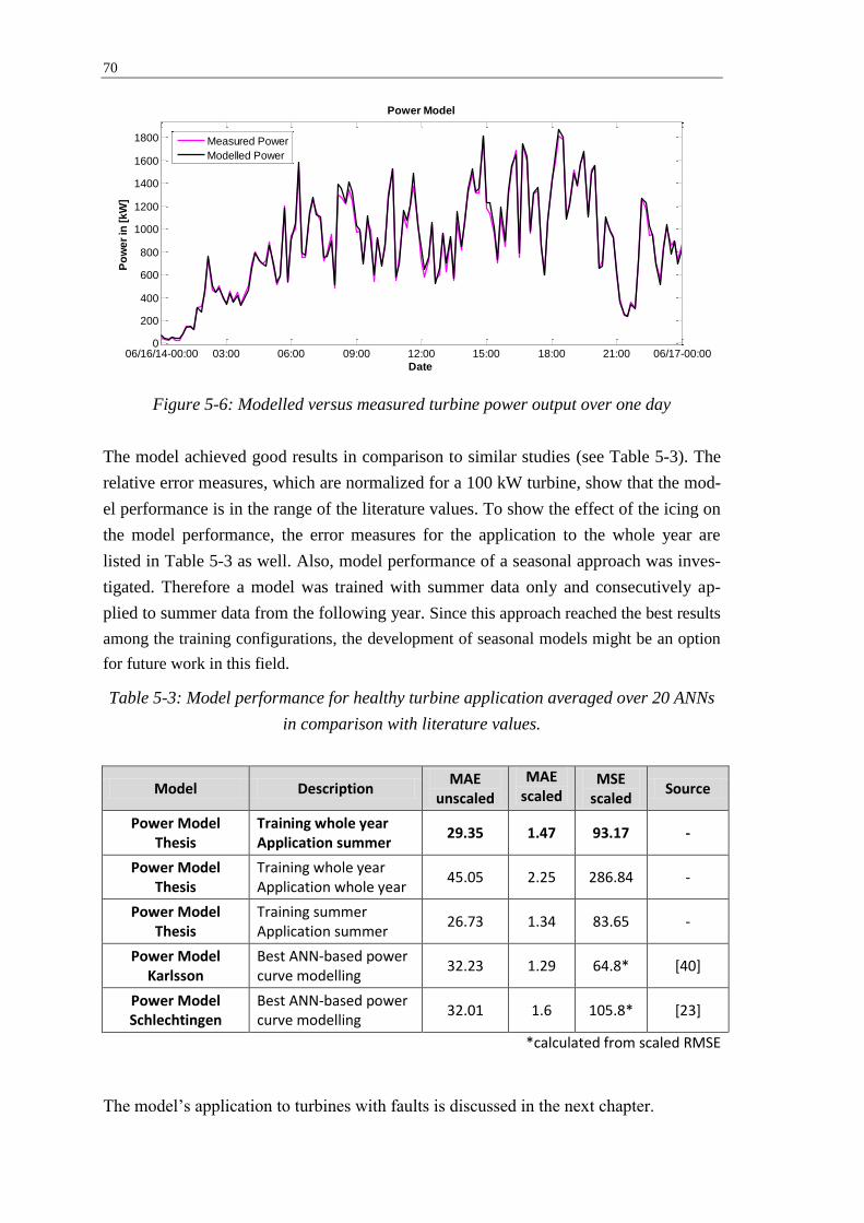
70
Figure 5-6: Modelled versus measured turbine power output over one day
The model achieved good results in comparison to similar studies (see Table 5-3). The
relative error measures, which are normalized for a 100 kW turbine, show that the mod-
el performance is in the range of the literature values. To show the effect of the icing on
the model performance, the error measures for the application to the whole year are
listed in Table 5-3 as well. Also, model performance of a seasonal approach was inves-
tigated. Therefore a model was trained with summer data only and consecutively ap-
plied to summer data from the following year. Since this approach reached the best results
among the training configurations, the development of seasonal models might be an option
for future work in this field.
Table 5-3: Model performance for healthy turbine application averaged over 20 ANNs
in comparison with literature values.
Model Description MAE
unscaled
MAE scaled
MSE scaled
Source
Power Model Thesis
Training whole year Application summer
29.35 1.47 93.17 -
Power Model Thesis
Training whole year Application whole year
45.05 2.25 286.84 -
Power Model Thesis
Training summer Application summer
26.73 1.34 83.65 -
Power Model Karlsson
Best ANN-based power curve modelling
32.23 1.29 64.8* [40]
Power Model Schlechtingen
Best ANN-based power curve modelling
32.01 1.6 105.8* [23]
*calculated from scaled RMSE
The model’s application to turbines with faults is discussed in the next chapter.
06/16/14-00:00 03:00 06:00 09:00 12:00 15:00 18:00 21:00 06/17-00:000
200
400
600
800
1000
1200
1400
1600
1800
Date
Po
we
r in
[k
W]
Power Model
Measured Power
Modelled Power

71
5.3 Model Application
The model presented above is applied to different failure cases. Firstly, the application
to the gearbox failure case 02 presented in the previous chapter is conducted. Then the
model is applied to turbines which are not sited in Sweden and showed different prob-
lems during operation. The aim is to investigate failure detectability from a system point
of view with the presented approach and draw conclusions for future applications. The
specifications of the power model which was applied in the case studies are summarized
in the table below:
Table 5-4: Summary of power model specifications
NARX ANN Configuration
Layer Hidden Output
Activation Function Sigmoid Threshold
Neurons 20 1
Inputs Wind Speed Avg. Wind Speed Std.
Nacelle Direction Ambient Temperature
Outputs Turbine Power Production
Training and Data Pre-processing
Trainings Algorithm Levenberg-Marquard
Trainings Period data available before failure
Filter Training Data Boundary Filter Cluster Filter
Skip Filter Curtailment (if available)
Training Philosophy best of 3 trainings / seasonal if necessary
Application and Anomaly Detection
MHD Averaging over one day
Data Sufficiency Limit at least 6h of data over one day
5.3.1 Power Study Case Gearbox Failure
Case Description
It was decided to investigate the gear failure case presented as study case two in the
previous chapter with the power model. The turbine got stuck after five years of opera-
tion and the gearbox was found to be responsible for that breakdown (compare chapter
4.3.2). The impact of the icing risk on the power model application can be studied in
this case because the turbine is located in Sweden. Therefore, the model was trained
with a full year of healthy data and then applied for the consecutive year, where the
failure occurred in the end of November.

72
Anomaly Detection
The familiar model application diagram shows high MHD values during the cold half of
the year. Three threshold violations can be noted in February/March and one just before
the gearbox breakdown in November (compare Figure 5-7).
Figure 5-7: Power model application for anomaly detection in a gearbox failure case
To be able to judge these model alarms, the predicted versus the measured power out-
puts responsible for the threshold violations are analyzed. They are shown in Figure 5-8.
Figure 5-8: Modelled versus measured power for three threshold violation periods
It can be observed that for each of the indicated malfunctions the power is predicted
below the actual power output. Before the model was applied it was expected that a
failure would manifest itself as a power over-estimation because it was assumed that
energy which is converted into power under normal conditions is dissipated due to an
increased mechanical friction in the gearbox during the failure. However, the result can
be explained when looking at the training and the application data-set. Figure 5-9 dis-
Jan/11 Feb Mar Apr May Jun Jul Aug Sep Oct Nov0
1
2
3
4
5
6
Date
Ma
ha
lan
ob
is D
ista
nc
e
Average Mahalanobis Distance
Normal Operation Limit
SCADA Alarms/Warnings
Data Missing
03/04/11 03/05 03/060
200
400
600
800
1000
1200
1400
1600
1800
2000
Date
Po
we
r in
[k
W]
Power Model
Measured Power
Modelled Power
02/11/11 02/12 02/130
200
400
600
800
1000
1200
1400
1600
1800
2000
Date
Po
we
r in
[k
W]
Power Model
Measured Power
Modelled Power
11/14/11 11/150
200
400
600
800
1000
1200
1400
1600
1800
2000
Date
Po
we
r in
[k
W]
Power Model
Measured Power
Modelled Power

73
plays both data sets. It can be observed, that the training data set covers a larger range of
parameters than the application data set. The reason therefore is the variable power
curve characteristics for the Swedish turbines. Since the model was trained to fit the
magenta input data it predicts on average lower value in comparison to the black appli-
cation data set which basically represents only the upper part of the training range. This
is confirmed by a look on the error distribution. In comparison to the training data set it
was shifted towards underestimation (compare Figure 5-10).
Figure 5-10: Shifted errors during application
Summary and Conclusion
This study case illustrates the challenges that come with variable ranges of parameters
and the limitations of ANNs. Under these conditions it is very difficult to judge whether
an alarm is issued due to abnormal turbine behavior or due to a shift in the range of pa-
rameters. A better method needs to be created to analyze the errors due to such skewed
input parameters, which change the distribution of the errors from the model.
5.3.2 Power Study Case Generator Bearing Failure
Case Description
The second study case analyzes two turbines which showed generator bearing failures.
Both turbines, direct drive concepts from a different manufacturer, showed both failures
in the generator bearing in February 2014. More detailed information, such as the
SCADA alarm records for example, were unfortunately not available. Also, there is no
generator bearing measurement available. Hence the possibility of detecting irregulari-
ties by applying the power model is investigated.
-1000 -500 0 500 10000
1000
2000
3000
4000
5000
6000
7000
Ins
tan
ce
s
Errors
Figure 5-9: Power curve of train-
ing and application dataset

74
The turbines come with a different SCADA system. On one hand the set of parameters
is a bit different and instead of the standard deviation of the ambient wind speed the min
and max values were used as a substitute. Moreover, there were many instances where
the SCADA data was missing. Therefore, the skip filtering was done slightly less ag-
gressively, removing only the data points directly before and after standstills of more
than three hours instead of 30 minutes. Lastly, these turbines do not report a curtailment
parameter in their SCADA system. Thus, it was not possible to reliably exclude the cur-
tailment data from the input and target sets. Moreover, the two turbines show consistent
power curves throughout the year. The anomaly detection results are presented next.
Anomaly Detection
Figure 5-11: MHD measure for both turbines until failure occurrence
The anomaly detection plots look very similar for both turbines. The MHD measure
says constantly beneath the threshold until about one month before the failure. Multiple
MHD peaks can be observed, each resulting in a threshold violation. It looks like a clear
failure indication and the amplitude of the peaks is surprisingly high. A closer look into
the data behind the peaks and the measured versus the modelled power output explain
the sudden increase of the MHD.
Oct/13 Nov Dec Jan/14 Feb0
2
4
6
8
10
12
Date
Ma
ha
lan
ob
is D
ista
nc
e
Average Mahalanobis Distance
Normal Operation Limit
SCADA Alarms/Warnings
Data Missing
Oct/13 Nov Dec Jan/14 Feb0
2
4
6
8
10
12
Date
Ma
ha
lan
ob
is D
ista
nc
e
Average Mahalanobis Distance
Normal Operation Limit
SCADA Alarms/Warnings
Data Missing

75
Figure 5-12: Measured values in relation to training data set and model
On the left side of Figure 5-12, the training power curve in relation to the data points
causing the high MHD values are shown. The location and arrangement of these data
points immediately remind of how curtailment manifests itself in the power curve, with
distinctly lower power output than the wind conditions would allow. On the right side of
Figure 5-12 the real measured turbine output in comparison to the modeled output is
presented. This behavior is observed for all the MHD peaks. It strongly suggests that the
power output was limited by an external source. Since there is no further information or
a curtailment indicator available, it is assumed, that the MHD peaks were caused by
manual power limitation.
Summary and Conclusion
From the behavior of both turbines it can be concluded that they are located on the same
site. The fact that the model alarms were triggered at the same dates confirms this. Since
there is no additional information available it can only be speculated whether the near
failure forced the operator to limit the power output, the power output limitation caused
the bearing failures through the volatile operation mode or both events have nothing to
do with each other. However, it is conspicuous that the failures occurred at the same
time for both turbines after being exposed to several of those sharp limitations of the
power output. To reliably judge these outcomes, further information, for example the
SCADA records, are required.
5.4 Discussion
The results from model validation and the study cases of Swedish turbines show that the
power approach is able to detect icing. Therefore, the training data should cover one
whole year, preferably where only little icing occurred. The data points in the training
set which are affected by the icing, will be filtered by the cluster filter, since they show

76
a clearly different relation between wind speed and power output. Consequently, the
model will issue alarms in application stage if the power output deviates from the model
output due to icing. This can be beneficial for operators, since icing is not easily detect-
able and can negatively influence a turbine’s performance and health. In fact, these re-
sults reveal that the power model is able to detect performance degradations due to
changes in the aerodynamic profile of the blade. This could mean that major blade fail-
ures, which have a corresponding impact on the aerodynamic blade performance, could
be potentially detected by the power model as well. However, this conclusion has to be
verified through further investigations.
The application of the power model in study cases has also shown that modelling a
global variable for component monitoring comes with several challenges. In general, it
can be said that additional information complementing the SCADA data itself is strong-
ly required for an appropriate judgement of the model output. This is also true for the
gearbox approach, but tracking the failure origin is much more challenging for the pow-
er approach, since there are much more potential sources from different parts of the tur-
bine that can make the measured power output deviate from the modelled one. Without
additional information it is very difficult to draw conclusions about the origin of the
deviation. Furthermore, the application of the power model to the Swedish turbines
showed the shortcomings of the presented method in terms of operating conditions that
deviate from the training year.
Also, the applied anomaly detection approach was originally developed to detect irregu-
larities in a local variable on which a failure has a relatively large impact. Consequently
the power model is able to detect anomalies with a comparable big influence on the
power output, such as for example icing. However, the method seems to be less suited
for indicating malfunctions that have only a small impact on power output but could
result in detectable energy losses over time. In other words, the power dissipated in a
bearing or a gear failure might be too small to be detected with the current approach,
especially when taking into consideration that the model’s mean absolute error is
around 30 kW (compare chapter 5.2). Therefore, an approach is suggested which identi-
fies deviations in the cumulated energy production over time.
It was shown, that the model’s error is normally distributed in the training year. This
means that a sum over all errors will always oscillate around zero in the training year. It
is assumed that a failure in one of the turbine components can disturb this balance, lead-
ing to a small shift of the failure distribution, which can be made visible by accumulat-
ing the errors. They would not sum up to zero but to a value below. However, it has
been observed that such a shift can also be caused by operating conditions that deviate
from the training year. Thus, a trend in the cumulated error could result from the operat-
ing conditions and cannot automatically be interpreted as sign of malfunction. But if

77
data from multiple turbines from the same site is available, their cumulated errors can
be compared, provided that they were trained with data from the same year. If the com-
parison of the cumulated errors reveals that one turbine behaves differently than the
majority it can be concluded that energy is somewhere dissipated, where it shouldn’t
and thus an inspection can be initiated. This approach is not applicable in case the pow-
er curves of the turbines are influenced by, for example icing, as it was the case for the
Swedish turbines. Thus, it was not able to modify this method, but the approach seems
promising and could help to identify failures with the help the power model.

78
6 Closure
This final chapter gives an overview of the thesis outcome, and wraps up the lessons
learned during the master’s thesis project. Various conclusions regarding the require-
ments and the key challenges for successful SCADA-based CM can be drawn from the
conducted analyses. They are presented and discussed in the following paragraphs.
Moreover, the method and outcomes are critically discussed to present a complete pic-
ture of the presented approaches. Finally, ideas for future work or further development
in the investigated field are presented.
6.1 Summary
To investigate the possibilities of SCADA data usage for component condition monitor-
ing in WTs, an ANN based normal behavior model was developed and applied to six
different gearbox failure cases. Two successful cases of failure detection were present-
ed, one indicating a malfunction long before the final component breakdown. This
shows that the analysis of SCADA data can be a helpful tool in component condition
monitoring.
In addition, the same methodology was applied to monitor a turbine by its performance.
The model was applied to two direct drive turbines with generator bearing failures.
Model alarms can be observed before failure occurrence, but more information com-
plementing the SCADA data is necessary to appropriately judge the model alarms.
Moreover, the model was found to be an effective tool for ice-detection on turbine
blades.
6.2 Discussion and Conclusions
Firstly, it has to be noted that for every investigation of SCADA data it is the data itself
that is the most decisive factor. Through the available parameters, the available failure
cases and additional information data determines the analysis like no other factor does.
In addition, the success of a CM approach relies on the data handling and the correct
application of the appropriate methods.
Based on the available data, the developed models were successfully applied for condi-
tion monitoring of WT components. The gearbox model was able to trigger alarm long
before the final component breakdown. This information can draw the operator’s atten-
tion to a developing malfunction and an appropriate maintenance strategy can be fol-
lowed. However, it has to be mentioned that the model was not able to issue alarms for

79
all available failure cases, but the method offers a cost effective supplement to existing
CM systems. Also, the power model can deliver useful information about turbine condi-
tion. Especially its application in the field of icing detection was discovered. The inves-
tigations revealed challenges of the approach, but also showed promising promise po-
tentials.
From a methodical point of view, it has been realized that the appropriate definition of
training and application data is a crucial point of the presented CM approach. Especially
since ANN output highly relies on the training input data. Firstly, training data has to be
free of failures so that the model is able to emulate normal operating conditions accu-
rately. Filtering approaches can be developed to ensure failure free training data, but at
the same time the whole range of normal operating conditions has to be covered to
avoid false alarms. This balance can be tricky to achieve and well suited data selection
and processing is the key. Defining the appropriate range of training data was found to
be much easier for the local variables than for the global power output, because local
variables are influenced by a limited amount of factors which can be overseen during
the selection process.
Data selection is not only critical for the training data set, but also the application data
has to be screened for data that would cause false alarms, such as for example SCADA-
communication errors. Moreover, any normal operation data that the model was not
trained for can be pro-actively excluded from the application set. An example would be
excluding curtailment data from the application data set. But this requires in depth
knowledge about the system since potential operating conditions which are not covered
by the training data have to be identified and excluded proactively. In addition, this
comes with the risk of excluding data that contains detectable traces of malfunctions. To
sum it up, the strong dependence of ANNs on the training data causes challenges in the
field of anomaly detection.
Furthermore, the availability of potential input and target parameters was identified as a
central point. This applies especially when modelling a local variable for component
monitoring. In general, it can be said that the more component related parameters avail-
able, the higher the chances to detect a component failure. More parameters simply in-
crease the probability that a malfunction manifests itself detectably in one of the addi-
tional measurements. It was observed that SCADA systems are using several measure-
ments for an internal monitoring approach which generates alarms and warnings based
on a comparison between the actual measurement and pre-set threshold. However, some
of these parameters were not extractable from the system. The availability of these
measurements would truly increase the possibilities for component monitoring. The
development of SCADA-systems in recent years shows a trend towards a wider range of
measurements which comes with new chances for SCADA based monitoring approach-

80
es. In addition, technological development has made it possible to store and analyze big
data without any major investments in the hardware infrastructure. The use of cloud
storage and parallel computing approaches can enable the storage and analysis of in-
creased amounts of data with multiple new measurements.
It was noticed that it is essential to have as much information as possible complement-
ing the raw data. Information about the turbine, its operating conditions and its failure
case is crucial when developing the anomaly detection approach. A close cooperation
with the operator is required and insights into maintenance SCADA records and
maintenance reports are very helpful. If this information is missing, it is difficult to
judge the model outcome and no effective feedback for a model adjustment is possible.
The exchange with operators has shown that there is a general interest in investigating
SCADA data for condition judgement. But generalization and commercialization of
such approaches is challenging due to several factors. Firstly, each turbine shows indi-
vidual operational behavior and thus it is difficult to develop a general model, which
can be applied to all turbines. Here lays the strength of the ANN application. Models
can adapt individual turbine behavior quite easily by using the turbines data for training.
Nevertheless, the application of one model to different turbines is still not easily possi-
ble in many cases. The work with SCADA systems from different operators has shown
that there is no specification of a standard set of measurements recorded by every tur-
bine. As long as this is the case, the CM based on SCADA will stay a highly individual
discipline and the development of generally applicable models is very difficult.
However, the positive results which were achieved, especially of the gearbox model,
show that operators can benefit from analyzing the SCADA data of their turbines. This
analysis does not aim to replace any of the existing CM systems but it is a cost effective
and elegant way to complement them. Further research and a parallel development of
the SCADA systems can help to realize the potentials of this approach. Such SCADA
analysis can definitively help operators to cope with the big amount of alarms and warn-
ings of standard SCADA systems. The models can indicate which ones to prioritize and
which ones to ignore. At the end of the day it is the operator’s duty to decide whether to
initiate maintenance actions or not and SCADA based models can support them.
6.3 Future Work
Based on the findings of this work further investigations might be interesting, including
the following:
The further development of the gearbox model under consideration of additional
thermal parameters, for example cooling specifications, could additionally in-

81
crease the quality of the presented model. Then, it would be worth investigating
the application of the model to different gearbox failure cases.
For successful early failure detection with the power model its anomaly detec-
tion method has to be adjusted. A possible solution could be the approach sug-
gested in chapter 5.4. The applicability then would have to be verified in differ-
ent in analyzing failures of different turbine components.
The implementation of the developed models in an integrated maintenance
scheme could utilize their potential benefit for turbine operators.
Hopefully the findings of this thesis can contribute to one of the suggested future fields.

82
References
[1] S. Gsänger; G. Hareli: New Record in Worldwide Wind Installations: More than 50 GW Additional Wind Power Capacity, Wind Power Worldwide Close to 370 GW. Bonn, 05.02.2015. URL http://www.wwindea.org/new-record-in-worldwide-wind-installations/ – Last check 2015-03-03
[2] EWEA (2014). EWEA: Wind in power: 2014 European statistics. URL http://www.ewea.org/fileadmin/files/library/publications/statistics/EWEA-Annual-Statistics-2014.pdf – Last check 2015-03-03
[3] Walford C. A. (2006). Sandia National Laboratories: Wind Turbine Relia-bility: Understanding and Minimizing Wind Turbine Operation and Maintenance Costs. URL http://prod.sandia.gov/techlib/access-control.cgi/2006/061100.pdf – Last check 2015-03-03
[4] P. Bangalore (2014). Chalmers University of Technology: Load and Risk Based Maintenance Management of Wind Turbines. [Online] Available: http://publications.lib.chalmers.se/records/fulltext/196744/196744.pdf
[5] K. Kim, G. Parthasarathy O. Uloyol W. Foslien S. Sheng P. Fleming (2011). NREL: Use of SCADA Data for Failure Detection in Wind Tur-bines. URL http://www.nrel.gov/docs/fy12osti/51653.pdf – Last check 2015-02-19
[6] Borchersen, Anders; Larsen, Jesper; Stoustrup, Jakob: Predicting Faults in Wind Turbines using SCADA Data. In: 51st AIAA Aerospace Sciences Meeting including the New Horizons Forum and Aerospace Exposition.
[7] P. Takoutsing et al.: Wind Turbine Condition Monitoring: State-of-the-Art Review, New Trends, and Future Challenges, Bd. 7. In: Energies: Open-access journal of related scientific research, technology development and studies in policy and management. Basel: MDPI, 2014, S. 2595–2630
[8] K. Fischer; F. Besnard; L. Bertling: Reliability-Centred Maintenance for Wind Turbines Based on Statistical Analysis and Practical Experience. In: IEEE transactions on energy conversion: A publication of the IEEE Power Engineering Society. 1. Aufl. New York, NY: IEEE, 2011 (27), S. 184–195
[9] Hau, Erich, 2014: Windkraftanlagen: Grundlagen, Technik, Einsatz, Wirt-schaftlichkeit. 5., neu bearb. Aufl. 2014. Berlin, Heidelberg: Springer Vie-weg, 2014 (SpringerLink: Bücher)
[10] Tavner P; Gindele R; Faulstich S; Whittle M; Greenwood D; Hahn B: Stu-dy of effects of weather & location on wind turbine failure ratesIn: Euro-pean Wind Energy Conference & Exhibition 2010: EWEC 2010: Warsaw, Poland, 20-23 April 2010, 2010, S. 255–258
[11] L. Bertling; P. Wennerhag; P (2012): Wind Turbine Operation and Maintenance: Survey of the Development and Research Needs. URL http://elforsk.se/Rapporter/?download=report&rid=12_41_ – Last check 2015-02-19

83
[12] B. Hahn; M. Durstewitz; K. Rohrig (2007). Institut für Solare Energieversorgungstechnik: Reliability of Wind Turbines: Experiences of 15 years with 1,500 WTs. URL http://www.researchgate.net/profile/Kurt_Rohrig/publication/46383070_Reliability_of_wind_turbines_Experiences_of_15_years_with_1500_WTs/links/0deec517c0f71963a0000000.pdf – Last check 2015-03-05
[13] Pérez; Márquey; Tobias; Papaelias: Wind turbine reliability analysis. In: Renewable Sustainable Energy Review (2013), Nr. 23, S. 463–472. URL http://ac.els-cdn.com/S1364032113001779/1-s2.0-S1364032113001779-main.pdf?_tid=5c6cd024-c320-11e4-8e07-00000aacb361&acdnat=1425550628_9c360e07521c8048370f18fea3edaa0c – Last check 2015-03-05
[14] Ribrant, Johan; Bertling, Lina Margareta: Survey of Failures in Wind Power Systems With Focus on Swedish Wind Power Plants During 1997–2005. In: IEEE Transactions on Energy Conversion 22 (2007), Nr. 1, S. 167–173
[15] Michael Wilkinson, Keir Marman Ben Hendriks (2011): Measuring Wind Turbine Reliability - Results of the Reliawind Project. – Aktualisierungsdatum: 2011-03-22. URL http://www.gl-garradhassan.com/assets/downloads/Measuring_Wind_Turbine_Reliability_-_Results_of_the_Reliawind_Project.pdf – Last check 2015-02-19
[16] J. Ribrant; L. Bertling (2006): Reliability performance and maintenance: A survey of failures in wind power systems. URL http://faculty.mu.edu.sa/public/uploads/1337955836.6401XR-EE-EEK_2006_009.pdf – Last check 2015-02-19
[17] F. Spinato; P.J. Tavner; G.J.W. van Bussel; E. Koutoulakos: Reliability of wind turbine subassemblies, Bd. 3. In: IET Renewable power generation. London: IET, 2009, S. 1–15
[18] E. Wiggelinkhuizen; Verbruggen, T.; Braam, H.; Rademakers, L.; Xiang, J.; Watson, S.; Giebel, Gregor; Norton, E.; Tipluica, M. C.; MacLean, A.; Christensen, A. J.; Becker, E.; D. Scheffler: CONMOW: Condition Moni-toring for Offshore Wind Farms. In: European Wind Energy Conference & Exhibition 2007. Milan: EWEA, 2007, S. 118–122
[19] Smolka, Ursula; Cheng, Po Wen: On the Design of Measurement Cam-paigns for Fatigue Life Monitoring of Offshore Wind Turbines. In: Chung, Jin S. (Hrsg.): The proceedings of the Twenty-third (2013) International Offshore and Polar Engineering Conference: Anchorage, Alaska, June 30-July 5, 2013: ISOPE-2013 Anchorage. [Cupertino, Calif.]: International Society of Offshore and Polar Engineers, 2013
[20] Ke-Sheng Wang; Vishal S. Sharma; Zhen-You Zhang: SCADA data based condition monitoring of wind turbines. In: Advances in manufactoring 2 (2014), Nr. 1, S. 61–69. URL http://link.springer.com/article/10.1007%2Fs40436-014-0067-0
[21] A. Zaher et. al.: Online Wind Turbine Fault Detection through Automated SCADA DataAnalysis, Bd. 12. In: Wind Energy. Chichester: Wiley, 2009 (12), S. 574–593

84
[22] Schlechtingen, Meik; Ferreira Santos, Ilmar: Comparative analysis of neural network and regression based condition monitoring approaches for wind turbine fault detection. In: Mechanical Systems and Signal Pro-cessing 25 (2011), Nr. 5, S. 1849–1875
[23] Schlechtingen, Meik; Santos, Ilmar Ferreira; Achiche, Sofiane: Wind tur-bine condition monitoring based on SCADA data using normal behavior models. Part 1: System description. In: Applied Soft Computing 13 (2013), Nr. 1, S. 259–270
[24] Yan, Yonglong; Li, Jian; Gao, David: Condition Parameter Modeling for Anomaly Detection in Wind Turbines. In: energies 7 (2014), Nr. 5, S. 3104–3120
[25] J. Xiang, S. Watson Y. Liu: Smart Monitoring of Wind Turbines Using Neural Networks, SEB'09. In: Howlett, Robert J.; Jain, L. C.; Lee, Shaun H. (Hrsg.): Sustainability in energy and buildings: Proceedings of the In-ternational Conference in Sustainability in Energy and Buildings (SEB'09). Berlin, Heidelberg: Springer-Verlag, ©2009, S. 1–8
[26] Rafiq, M.Y; Bugmann, G.; Easterbrook, D.J: Neural network design for engineering applications. In: Computers & Structures 79 (2001), Nr. 17, S. 1541–1552
[27] Müller, Berndt; Reinhardt, J.; Strickland, M. T., 1995: Neural networks: An introduction. 2nd updated and corr. ed. Berlin, New York: Springer, 1995 (Physics of neural networks)
[28] S. Haykin, 2009: Neural networks and learning machines. 3. Aufl. Upper Saddle River, N.J: Pearson, 2009 (Pearson International Edition)
[29] Beale, Mark; Hagan, Martin; Demuth, Howard (2015). The MathWorks, Inc.: Neural Network Toolbox™: User's Guide. URL http://www.mathworks.com/help/pdf_doc/nnet/nnet_ug.pdf – Last check 2015-06-26
[30] Kusiak, Andrew; Zheng, Haiyang: Optimization of wind turbine energy and power factor with an evolutionary computation algorithm. In: Energy 35 (2010), Nr. 3, S. 1324–1332
[31] Kusiak, Andrew; Li, Wenyan: The prediction and diagnosis of wind tur-bine faults. In: Renewable Energy 36 (2011), Nr. 1, S. 16–23
[32] Kusiak, Andrew; Verma, Anoop: Analyzing bearing faults in wind turbines: A data-mining approach. In: Renewable Energy 48 (2012), S. 110–116
[33] Garcia, Mari Cruz; Sanz-Bobi, Miguel A.; del Pico, Javier: SIMAP: Intelli-gent System for Predictive Maintenance. In: Computers in Industry 57 (2006), Nr. 6, S. 552–568
[34] Schlechtingen, Meik; Santos, Ilmar Ferreira: Wind turbine condition moni-toring based on SCADA data using normal behavior models. Part 2: Ap-plication examples. In: Applied Soft Computing 14 (2014), S. 447–460
[35] The MathWorks, Inc.: Neural Network Toolbox: Create, train, and simu-late neural networks. URL http://www.mathworks.com/products/neural-network/ – Last check 2015-07-01

85
[36] Agresti, Alan; Franklin, Christine A., 2014: Statistics: The art and science of learning from data. Third edition. [United Kingdom]: Pearson, 2014
[37] Paliwal, Mukta; Kumar, Usha A.: Neural networks and statistical tech-niques: A review of applications. In: Expert Systems with Applications 36 (2009), Nr. 1, S. 2–17
[38] NIST (2003). NIST: Engineering Statistics: Handbook. URL http://www.itl.nist.gov/div898/handbook/index.htm – Last check 2015-07-15
[39] De Maesschalck, R., Jouan-Rimbaud, D. & Massart, D. L., 2000. The
Mahalanobis Distance. Chemometrics and Intelligent Laboratory Sys-
tems, 50(1), pp. 1-18.
[40] Karlsson, Daniel (2015). Chalmers University of Technology: Wind Tur-bine Performance Monitoring using Artificial Neural Networks: With a Mul-ti-Dimensional Data Filtering Approach. Master’s thesis in Sustainable Energy Systems
[41] Friis Pedersen, T.; Gjerding, S.; Ingham, P.; Enevoldsen, P.; Kjær Han-sen, J.; Kanstrup Jørgensen, H., 2002: Wind turbine power performance verification in complex terrain and wind farms, 2002 (Contract ENS-51171/97-0045)