ce RADC-TR4140In-House ReportMarch 1981

SBASIC DESIGN PRINCIPLES OFSELECTROMAGNETIC SCATTERING

MEASUREMENT FACILITIES

Richard B. Mack

APPROVED FOR PUBLIC RELEASE; DISTRIBUTION UNLIMITED

D C_F_-CTE~

ROME AIR DEVELOPMENT CENTER ' SEP9 198 j;Air Force Systems Command

*' Griffiss Air Force Base, New York 13441 D

o4

, -

This report has been reviewed by the RADC Public Affairs Office (PA)and is releasable to the National Technical Information Service (NTIS). AtNTIS it will be releasable to the general public, including foreign nations.

RADC-TR-81-40 has been reviewed and is approved for publication.

APPROVED:

PHILIPP BLACKSMITH, Branch ChiefEM Techniques BranchElectromagnetic Sciences Division

APPROVED: P 0

C. SCHELL, ChiefElectromagnetic Sciences Division

FOR THE COMMANDER:

JOHN P. HUSSActing Chief, Plans Office

If your address has changed or if you wish to be removed from the RADC mailinglist, or if the addressee is no longer employed by your organization, pleasenotify RADC (EEC), Hanscom AFB MA 01731. This will assist us in maintaininga current mailing list.

Do not return this copy. Retain or destroy.

'5

UnclassifiedSMCIRITY CLASS'IICAT ION Of THg I% 41E (Wy,., Dera, .trd)___________________

REPOT DCUMNTATON AGEREAD INSTRUCTIONSREPOT__________NPAG BEFORE COMPLETING FORM

1 JPRAD .T 8-4D n2.G V A jSSION NO. 3. RECIerJTS CATALOG NUMBER

S. TYFE OF REPORT & PERIOD COVERED

SIC arSIGN & NCIPLES OF EJCTRO- In-House Report

C:7 6. PERFORMINO ORO. REPORT NUMBER

Richard 13. lackNI

Hanscom Air Force Base 44Massachusetts 01731 3A 4

9 ~ Unclassified

16 DISTRIOUTION STATEMENT (of this ~oU /

Approved for public release; distribution unlimited.

17 DISTRIBUTION STATEMENT (of th. abstract entered In Block 20, #1 different from, Report)

is. SUPPLEMENTARY NOTES

*Formerly RADC

RADC Project Engineer: R~onald G. Newburgh (EEC)'9 KEY WORDS (ConIlnue an reverse aide it noc..ary and Identify by block number)

Elect romagnetic scatteringRadar cross sections

40 AVTRACT (Continue on tao.,. side if necessary and Identify by block nuat bet)

_..rypical experimental configurations that are used for measuring radarscattering are analyzed with simplified forins of basic elect romagnet ic prin-ciples to show how the experimental facility design affects measurementcapability and the accuracy of the measured results. The discussion includeseffects of a nonuniform field over the model space, the measurement distancefrom the scattering model, multiple reflections from walls of a chamber orfrom nearby objects, interference from mnodel support structures, and thle

DD I JAN 73 1473 EDITION OF I NOV 65 1S OBSOLETE Unclassified ~~'SSECURITY CLASSIFICATION OF THIS PAGE (I*bon, Data Entere)\(,

" ' " UnclassifiedSrCU M CASSFICAIONOF HISPAGE(I7,.n Date 5nteuod)

20. Abstract (Continued)

-- effects of forward scattering. Guiding principles are developed for choosingand designing the important components of a scattering measurement facilitysuch as the transmit/receive antennas, the rf power sources, model supportstructures, and transmission line component assemblies so that measurementaccuracy is maximized. Simple experimental procedures are given forevaluating a given measurement setup. Emphasis in the report is placed onillustrating the principles with numerical examples.

II

I

i 1 Unclassified

SLOO LtS A1%O G K-01

- r

A-+ocosallon ?or

?PT!S GRA IDTC TAB "T"Unannounced ,T++ ustification U ,

By SEP 9 1981'Distribution/

Availability Codes WAvail and/or D

Dist spobcal

Contents 41. INTRODUCTION 7

2. BASIC EM SCATTERING PRINCiPLES 92. 1 Electromagnetic Similitude 102.2 The Far Field of the Model 122.3 The Incident Field Over the 111odel Space 172.4 Cancellation of the Background Signal 212.5 Model Range Power Relations 24

3. THE CHAMBER 283. 1 Antenyta/RF Components Shield 283.2 Removable Access Ports for Shielding Wall 313.3 Chamber Reflections 313.4 Reflections from Back Wall 36

3.4. 1 Power Reflected to the Receiver With NoScatterer Present 36

3.4. 2 Fields Over the Model Space, No Scatterer 3V,3. 4. 3 Power at the Receiving Antenna Due to Forward

Scattering by Model 3')3. 5 Estimated Interference from Multipath Signals 4'3. 6 Absorber Characteristics 43

4. TRANSMIT/RECEIVE ANTENNAS 484. 1 Practical Approximations to the Optimum Antenna 50

'4.2 Tunnel Antennas .53

5. MODEL SUPPORT STRUCTURES 545. 1 The Mount 565.2 Basics of Polyfoam Columns 56

5.2. 1 Column Diameter vs Model Weight 585.2.2 Backscatter-Cylindrical Column 58

3

I . .

Contents

5. 2.3 Backscatter-Truncated Cone Column 605. 2.4 Forward Scattering from Polyfoam Columns 60

6. RF POWER SOURCES 63

6. 1 Cancellation Requirements 636. 2 Frequercy Stability Requirements 64

7. TRANSMISSION LINE COMPONENTS 69

8. TYPICAL FACILITY PERFORMANCE 76

REFERENCES 79

Illustrations

1. Geometry for Determining Phase Error Due to FiniteMeasurement Distance 14

2. Backscatter Pattern of 10. Square Plate at VariousMeasurement Distances '6

3. Backscatter Pattern of 10X Square Plate in VariousField Tapers 2

4. Antenna/RF Equipment Shielding Options 305a. Port Arrangemei.t of Full Wall Shielding 325b. Port Arrangement for Tapered Chamber 326. Details of Port Sections 337. Geometry Illustrating Forward Scattering 40

8. Geometry for Estimating Yultipath Reflections 41

9. Theoretical Pattern-Circular Aperture, UniformIllumination 43

10. Pyramidal Absorber Reflectivity (Normal Incidence) 4511. Wideangle Reflectivity-Pyramidal Absorber 46

12. Lateral Field Variation at R = 2D 2 /X 1,,013. Three Antenna Approximation to Optimum 5214. Hall Power Distances at Model Space for 3 Antenna

Approximation to Optimum 5215. Results of Using Tunnel to Reduce Far Out Radiation 5416. Typical Model Support Structure 5517. Variations of Power Over Model Space Due to Forward

Scatter from Absorber Shield 6218. Single Antenna Backscatter Equipment 70

4

Illustrations

19. Dual Transmit/Receive Antenna Scattering Equipment 72

20. Equipment Racks 74

21. Mlnimum Measurable Cross Sections with :b1 dB ErrorWith Typical Backscatter Facility 78

22. Maximum Model Size, Maximum Antenna Size, and HalfPower Beam Distances for I = I GHz to 40 GHz atVarious Measurement Distances 78

Tubles

1. Error in Maximum of Backscatter Pattern Due to FiniteMeasurement Distance 17

2. Scattering Pattern Errors for Various Cancellation Levels 23

3. RCS Error vs Background Cancellation 24

4. Forward Scatter to Backscatter Ratios for a Sphere 35

5. Approximate Pyramidal Absorber Reflection Coefficientsat I GHz 47

6. Normal Incidence Frequoncy Behavior, Pyramidal Absorber 47

7. List of Transmission Line Components 75

8. Assumed Typical Equipment Parameters and MinimumMeasurable Cross Sections 76

£]

V?

i$

V

NPAGE

~Basic Design Principles of ElectromagneticScattering Measurement Facilities !

1. INTRODUCTION

The purpose of this technical report is to examine the basic electromagnetic

principles that govern the design of electromagnetic scattering measurement facil-ities. Special emphasis is placed on the practical application of the principles andon their practical meaning in determining the effects of the facility design on meas-urement accuracy. Although the discussions are not specifically restricted to any

frequency range, they are implicitly directed toward the frequency range of 1 GI-12to 40 GHz,

Likewise, most of the discussions apply to short pulse or other types of scat-

tering measurements but are implicitly directed toward CW cancellation systems.The principles discussed apply equally to measurements made on an outdoor facil-ity or to measurements on an indoor range where the free space environment is

approximated by a microwave anechoic chamber. Ideally, the overall design param-

eters of the facility would be dictated by the types of measurements anticipated, themodel sizes, frequency ranges. cross section levels, the degree of automation

desired. etc. In reality. such parameters can rarely be specified in advance.

When the facility is to be used in an R & D environment t.he anticipation of futuredesirable projects is even less precise. In such a situation it is well to recall that

~an arbitrarily imposed set of design parameters is in fact an advanced statement

~(Received for publication 19 February 1981)

7I* .

4xNI

Z, df what the facility will never be capablt of measuring. The importance o! thisconsideration is that a specified set of ,e'jign parameters can frequently be met

by restrictive designs that largely prohibit the facility's even occasional use for

projects that fall outside of the origina . parameters.

The alternative approach is to design the facility for maximum versatility, and

this design philosophy is generally followed in the present discussion.

There are some implications of the "design for maximum versatility" philos-

ophy. For example, the advantages in terms of minimum measurable cross sec-

tions of being able to measure a model at the shortest range consistent with being

in the model's far field are discussed in the next section. If the chamber design is

focused on producing a quiet zone of some limited volume centered at one spot of

the chamber, the advantages of optimizing the measurement range for each scat-

terer are lost. Similarly, if cheaper absorber of lower quality or having polariza-

tion sensitivity is used on side walls of the chamber, the ability to make measuwe-

ments at bistatic angles or with other than horizontal and vertical polarizations

may be severaly limited. The net result is that a versatile chamber to be used forelectromagnetic (EM) scattering measurements cannot take full advantage of recent

advances in chamber design.Note that in this respect, the requirements for a scattering measurement range

and, in particular, for an anechoic chamber to be used for scattering measurements,differ from those of an antenna measurement range or chamber. The antenna caseinvolves one way propagation paths, generally much higher power levels at the

receiver, and never requires bistatic measurements. Hence, the quiet zone ap-

proach to design of an antenna range or chamber can lead to a very versatile facil-

ity.

The frequency range is another fundamental consideration. The discussion

herein is directed toward operation over tl,e band of 1 GHz to 40 GHz. The general

guides for these limits are that smaller targets can be measured without modeling

at L-Band, while larger real system targets, such as airplanes viewed with an

L-Band radar, require high model measurement frequencies if the scaled model isto be of a convenient size. For example, since scaling is linear with wavelength,

a 40 ft target at 1 GHz becomes a Itt model at 40 GHz.The required far field measurement distance is proportional to the square of

the maximum dimension of the model and inversely proportional to the wavelength

and, hence, only 1/40 of that required for the full scatterer in the above example.

An additional consideration in choosing the general frequency range is that,based on the manufacturer's literature, pyramidal absorber with reflectivity levels

specified at 1 GHz first improves as the frequency is increased, but then deterio-

rates in performance as the frequency is raised, until, at 40 GHz its reflectivity

is approximately the same as at 1 GHz. In addition, a -40 dB reflectivity level

8

specified at I GHz still permits useful but lower quality measurements in thechamber down to 300 MHz.

An electromagnetic scattering measurement facility can be divided into the

following set of subsystems:

1. The range (or chamber)

2. Model mounts

3. Transmit/Receive antennas

4. RF transmitting sources

5. RF plumbing

6. Receiving equipment

7. Data handling equipment

Each subsystem has its own set of technical requirements and design tradeoffswithin the constraints of the overall facility parameters. An understanding of the

Individual subsystem tradeoffs will frequently permit a combination of them to be

played against each other to yield more accurate results, or even to perrit reliable

measurements of scatters that could not be accommodated by a given facility if a

rigid application of fixed criteria were made.

Section 2 gives a brief review of the basic laws governing the accuracy of radar

scattering measurements, and of the laws that define the measurement capability of

a given facility. The following sections contain detailed discussions of each subsys-

tem except the receiving equipment and the data handling equipment. Choice ofreceiving and data handling equipment are basically not electromagnetic concerns

and are determined primarily by state of the art commercial products that are

available within budgetary constraints. Primary requirements of the receiver arethat it be stable and very sensitive. Typical commercial receivers currently avail-

able have minimum detectable signal levels of -70 dBm at 40 Gi-z improving to

-110 to -120 dBrn at 1.0 GHz and these are very suitable. The receiver also shouldbe capable of measuring phase as well as power or amplitude, and should have out-

puts that are compatible with existing analog recorders for recording both phase

and amplitude. It is also highly desirable that the receiving equipment have a cap-ability of at least digitally storing the input data on tape for later computer process-

ing, because nearly all measured scattering data is relative data and frequently

requires normalization and scaling to actual operational frequencies.

2. BASIC EM SCAflERING PRINCIPLES

The production of high quality measured data from a given scattering measure-ment facility requires the careful application of only a few relatively simple rules,

but these basic rules must be applied with understanding if good results are to be

9

iFw

obtained with even the highest quality facility. These basic principles, in turn,impinge on the facility design becr.use the facility should be designed, insofar as

possible, within limitations of physical and budgeting restraints to enhance the

measured results.

The basic principles tnat govern scattering measurements are summarizedbelow and discussed in the following subsections. Examples given are specificallyfor free space backscatter facilities but appropriate versions of the principles

apply to all types of EM scattering facilities.

The principles are:1. Linear passive electromagnetic systems can be scaled up or down in fre-

quency, with linear dimensions scaled directly proportional to the wavelength orinversely as the frequency. Areas scale as the square of the wavelength or in-

versely as the square of the frequency.

2. Measure..ents of the scattered fields must be made in the far field of thescattering target.

3. The incident field over the space to be occupied by the scatterer must be aclose approximation to a plane wave.

4. Background signals from wall reflections, leakage, etc., must be reducedby some means to levels that do not introduce unacceptable errors into the lowestcross sections to be measured. The reduced levels of background signal must bemaintained during the course of a measurement.

5. Power relationships in EM scattering measurements are governed by theradar equation. For a given experimental setup this equation defines the smallest*.ross section that can be measured with a specified error.

2.1 Electromagnetic Sindlitude

The laws of electromagnetic similitude say that electromagnetic systems willgive equivalent results at an, frequency as long as all linear dimensions of the

system are scaled in an inverse proportion to the frequency. In air, linear dimen-sions are simply directly proportional tk, the wavelength.

This simple property of electromagnetic systems makes possible the use ofmodel measurement ranges. For example, a real radar target having a maximumdimension of 40 ft will yield the same relative scattering pattern at L-Band (I GHz)as an accurately constructed model having I ft maximum dimensions and measuredat 40 GHz. Similarly, a 4 ft model could be used at 10 GHz or a 20 ft model at2 GHz. The relationship is

p

1. Blacksmith, P., Hiatt, R. E., and Mack, R. B. (1965) Introduction to radar

cross section measurements, Proc. IEEE 53:901-920.

10

L2 (X2 / 1 )Ll (f1/f 2)Ll (1)

where L2 represents linear model dimensions at frequency f 2 and wavelength X2,

and Li represents linear model dimensions at frequency f1 and X1. Clearly,linear media and linear materials are assumed.

The word "accurately" is underlined because it is an important key to measur-

ing the same scattering pattern with different models scaled to represent different

real operating frequencies. Accurately means all of the details including the in-

terior of openings, gaps, stores, and any surface over which surface fields can

exist and contribute to the reradiated field. Accurately also means tolerances and

these also scale according to Eq. (1). Thus, it the model is to represent a real

scatterer within X/20, tolerances of an X-Band (10 Gliz) model must be -0. 050 in.

and tolerances of a 40 GHz model must be no poorer than *0. 0125 in.

The costs of constructing a model are at least inversely proportional to the

tolerances. Hence, it is common practice to make estimates of details that are

too small to affect the scattering pattern, and to estimate the effects of reduced

tolerances on major features of the scattering pattern prior to specifying the

model's tolerances.

Real radar targets at UHF, VHF, and HF have many details that do not con-

tribute significantly to the scattering pattern, and can therefore be represented by

very simple models. However, at L-Band and higher frequencies, nearly all de-

tails contribute and must be included in the model If the model is to be an accurate

representation of the real target.

A statement commonly made is that there is generally poor agreement between

the relative scattering patterns frcm a model measurement and those from the real

scatterer. The differences are very frequenly caused by failure to include suf-

ficient details and accuracy in the model.

As applied to i adar scattering measurements, Eq. (1) is used three ways.

First, if a fixed :..odel measurement frequency is available, Eq. (1) defines the

model size to represent a full size system at a given full size radar frequency.

Secondly, if a model is available, Eq. (1) defines the measurement frequency torepresent a given full size target and radar. Thirdly, it model measureme:nt re-

suits are already available from a model of given size me..ured at a given model

frequency, Eq. (1) defines the Null system target size and radar frequency to which

the results apply.

The absolute radar cross section of a scatterer is an area and hence, varies

as the square of the wavelength or inversely, as the square of !be frequency for

scaled systems,

a 2 22 =(2/'Y) al 1 f/Y ) al (2)

where 2 is the radar cross section at frequency f2 and wavelength Nt and a is the2 2' X212(tE 2

w iradar cross section at frequency f1 and wavelength 21 Note that while scaling EMscattering systems for measurements to higher frequencies offers the advantage of

smaller models, the higher frequency model range must be capable of measuringsmaller cross sections. For example, a low cross section target at L-Band (I GHz)

might have an radar cross section (RCS) of 0. 1 m 2 at some aspect. At X-Band(10 GHz) its model's RCS at this aspect would be 10"3 i 2 , and at 40 GHz an appro-

priately scaled model would have an RCS of 0.25 (10 " ) m2 . An airplane might

have an RCS of 400 M2 at some aspect. Its X-Band model would have an RCS of

4 m2 at the same aspect and its 40 GHz model an RCS of 0. 25 m .

2.2 The Far Field of the Model

The relative scattering patterns and the radar cross sections of the model mustbe measured at a sufficient distance H from the model to insure that the measuredresults are Independent of R. This is commonly referred to as being in the far

field of the model.Mathematical statements of the far field requirements are easily derived from

the Kirchoff-Huygens formulation for calculating the scattered fields. 2 ' 3 In this

formulation the scattered magnetic field is given by

HS T- f 16XioXVe' irlrdS (3)s

where the surface of integration is the surface of the scatterer and a closed surface

at infinity (over which the integral is zero), fi is a unit normal to the surface, Httis the total tangential field on the surface of the scatterer, and r is the distance

from the observation of measurement point, the transmit/receive antenna of a

model backscattering range, to a current element on the surface of the scatterer.Equation (3) contains no approximations, it gives the scattered field everywhere

outside of a perfectly conducting scatterer.

2. Silver, S. (1949) Microwave Antenna Theory and Design, Vol. 12, RadiationLaboratory Series, McGraw-Hill Book Company, Chap. 6.

3. Kerr, D. E. (1951) Propagation of Short Radio Waves, Vol. 13, RadiationLaboratory Series, McGraw-Hill Book Cbmpany, Chapts. 4 and 6.

12

Consider the gradient:

V- eikr no k - (4)

and the scattered field becomes

ils f . f X (fiX it(r + 1)ekrdS (5)s tS

Since we are interested in the field at relatively large distances from thescatterer, little error is introduced by replacing r by R, the distance from the

measurement point to the center of the scatterer, in the amplitude. R is i.depen-dent of the integration so that

s I'k 1e-ikr]=- [+Li 1 f to X(iXt) dS . (6)

R SI

Thus, In general there exist two components of the scattered field which differ

In phase by 900.The phase requires a more delicate treatment, From Figure 1 the difference

in path length to a measurement point located a distance R from the center of thescatterer between a current element at the center of the scatterer and one at x' is I

so that

r + I = (RI +x12)12 = l(1+ x 2 /R 2) 1 2 = R(I+x'2 /2R 2 ) (7a)

= R + x 2 /2R . (7b)

Then the field becomes

ffs 2s . (ik + I/R) f [no X (fi X )J ekx/2R dS (7c)

8

Since the scattered field at any measurement point is complex with both an

amplitude and a phase, separate conditions must be placed on each to insure thatthe measurement distance from the scatterer is sufficient to guarantee that there is

13

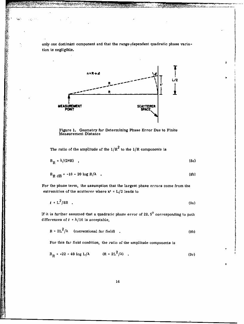
only one dominant component and that the range:dependent quadratic phase varia-

tion is negligible.

- na+* --- - - -- -L/2

- - - - """I

MEASUREMENT SCATTERERPOINT SPACE

Figure 1. Geometry for Determining Phase Error Due to FiniteMeasurement Distance

The ratio of the amplitude of the 1/fl to the 1/R components is

F R e /reR) (8a)

RR d=-16 - 20 log R/X. (8b)

For the phase term, the assumption that the largest phase errors come from theextremities of the scatterer where x' = L/2 leads to

I = L 2 /8R (9a)

If it is further assumed that a quadratic phase error of 22. 5 corresponding to pathdifferences of I = X/16 is acceptable,

R = 2L2 / A (conventional far field) . (9b)

For this far field condition, the ratio of the amplitude components is

RR = -22-40 log L/( 2L2/= ) 2 (9c)

14

Except-in cases where the conventional far field criterion is applied to scat-

terers that are small compared to the wavelength, its application generally insures2that the 1/R components are negligible compared to the 1/R components of the

field. For example, if I/X = 1, R = -22 dB and the error created in the measured

cross section is (see Blacksmith, et al, Figure 3) approximately *0. 75 dB; for

L/X 2, RR = -34 dB and the possible error in measured cross sections is approx-Imately ±0. 2 dB. If the scatterer has three or more wavelengths in its maximum

dimension, measurements at distances specified by the conventional criteria will

result in errors of *0. 1 dB or less in measured cross sections due to the neglected

field components.

Whether the criterion of Eq. (9b) is sufficient to keep the quadratic error with-

in acceptable limits depends on how heavily the scatter in question weights the cur-

rent elements at its extremities. For a given scatterer this also is a function of Ithe orientation of the scatterer, In general. A

Figure 2 shows examples of quadratic phase error due to finite measurementdistances in the backscatter pattern of a square flat metal plate of IOX on a side.

2,3Patterns in Figure 2 were calculated from physical optics ' for distances R = pwith p = 1/2, 1, 2, 4, and infinity. As can be seen from Figure 2 the largest

errors are introduced near the first null and first side lobe of the scattering pat-

terns. Even at substantially reduced distances, the error effects decrease atangles away from the broadside direction, even though the overall pattern levels

are lower at the SE angles. Also, doubling of the measurement distance increasesthe null depths by approximately 6 dB.

Beyond the center of the first side lobe through the third side lobe the pattern

at R 2L /X gives a pattern that is within 0.5 dB of the ideal one except very nearthe nulls; at angles beyond the third side lobe the approximation is better. Sim-

ilarly, the criterion R = L2 /X gives a pattern within approximately I dB of theideal one at and beyond the first side lobe the approximation is better. Similarly,

2the criterion R L /2X gives a pattern within approximately 1 dB of the idealone at and beyond the first side lobe except near the nulls. Effects of the quad-

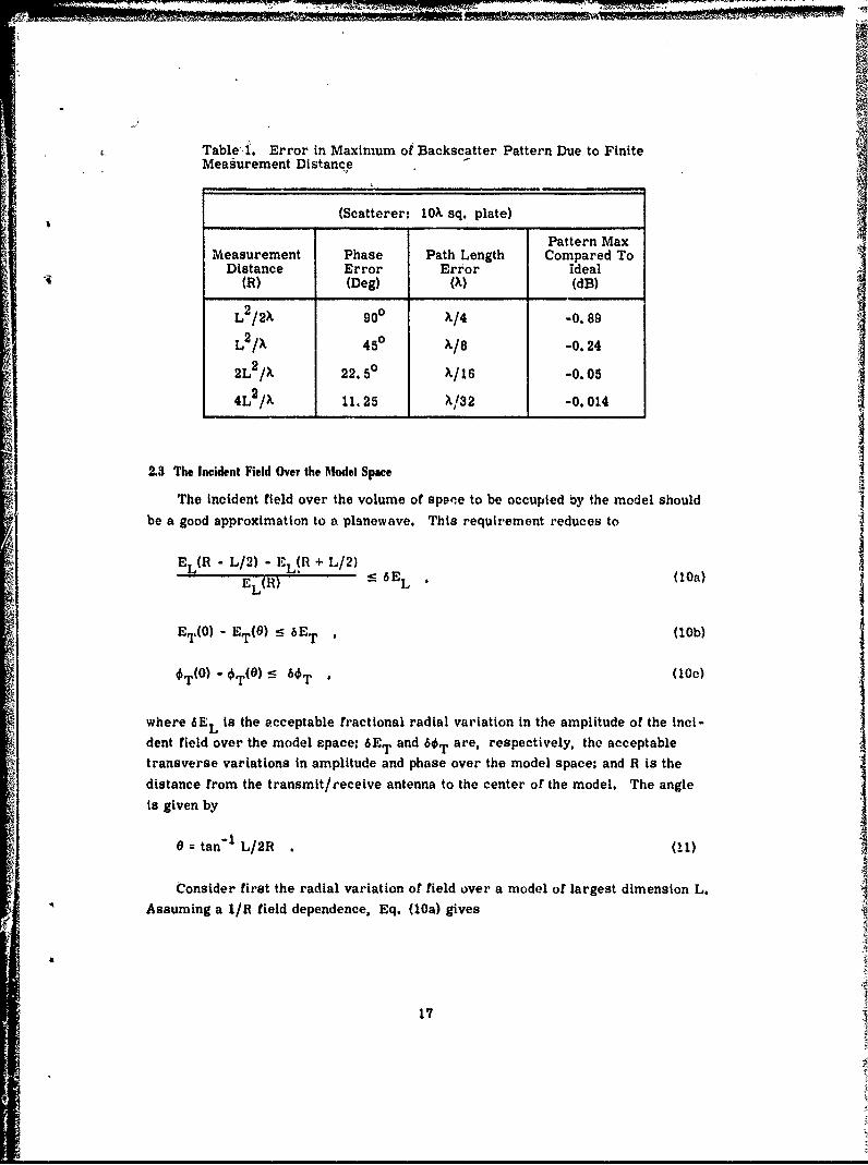
ratic error on the pattern broadside maximum are summarized in Table I.Note that the preceding discussion of backscatter from a square plate assumes

the incident field to be a planewave and only the receiving distance to be finite.

Experimentally, it is usually very simple to determine if a given measurementdistance R is sufficient to obtain a scattering pattern within a desired error toler-

ance. The procedure is to measure the pattern at a chosen distance, move thescatterer toward or away from the transmit/receive antenna and remeasure the

pattern. If pattern differences are within acceptable limits, the closer distance isadequate. This procedure is especially useful when scattering patterns must be

15

measured over a *wide power range and the lower powers are too close to thereceiver noise leveY to permit use of the conventional far field criterion.

0

-12-14

-18

.W -20

'0C -24

-,26. R.4L2A

.3 -2

~-38

-42 --4-36

0ID 1* 20 30 5* 6* 7* so SP t

DEGREES FROM BROADSIDE

]Figure 2. Backscatter Pattern of lOX Square Plate at Various Measure-ment Distances

16

10

Table 1. Error in Maximum of Backscatter Pattern Due to FiniteMeasurement Distance

(Scatterer: 10k sq. plate)

Pattern MaxMeasurement Phase Path Length Compared To

Distance Error Error ideal(R) (Deg) (X) (dB)

L2 /2X 900 X/4 -0.89

L 2 /. 450 X/8 -0.24

2L 2 /x 22.50 X/16 -0.05

4L2 /X 11.25 X132 -0. 014

2.3 The Incident Field Over the Model Space

The Incident field over the volume of spen'e to be occupied by the model should

be a good approximation to a planewave. This requirement reduces to

EL(M - L/2) - ELR + L/2)EL(fl) - 6 EL (1Oa)

L*

ET(O) - ET(O) E- 6E T , (10b)

OT(0) - OT(0) _ 6 6T * (10c)

where 6EL is the acceptable fractional radial variation in the amplitude of the inci-

dent field over the model rpace: 6 ET and 60T are, respectively, the acceptabletransverse variations In amplitude and phase over the model space. and R is thedistance from the transmit/receive antenna to the center of the model. The angle

Is given by

0 = tan "I L/211 (t

Consider first the radial variation of field over a model of largest dimension L.

Assuming a 1/11 field dependence, Eq. (10a) gives

17

6 E _ 1/(R - L/2) - 1/(R + L/2) = Lli,6EL I (12a)hR 1 - (L/2R) 2 (2a

L/R (12b)

The-transverse field is given by the antenna pattern of the transmit/receive

antenna. For a circular aperture and uniform illumination the pattern is given by

Skolnik (Chapter 7)4

ETC = (D sin=) (13)

Using small angle formulas,

-I1sin 0 A 0 = tan 1 L/2R 1 0

so that

ETC T (circular aperture uniform illumination) (14a)

6 ETc= I -ETc (14b)

Half power beamwidths are given by

0 1/2C - (58. 5 A/D) ° (circular aperture uniform illumination) (14)

A useful series for Jl(x)/x is

J1 (x ) x2 +x 4 x +(5: 8 8-4 2.24. 48 + .... (15)

4. Skolnik, M. 1. (1962) Introduction to Radar Systems, McGraw-Hill Book

Company, Chapts. 1 and 7.

18

The phase Is typically nearly constant ac re.Ss the main beam out to the, halt

power points. Hence, if the amplitude illumination is smooth-over the scatterer

: space the phase will also be smooth.,Many combinations can be used to satisfy Eqs.- (10a) to (10c) and all are legit-

imate as long as the far field distances of the scattering model are not violated.These include measuremcnts in the nea-' field of the antenna if the model is small,

or the antenna focused in the near field with the scattering m-idel located at the

focal region.

The actual criteria for Eqs. (10a) to (10c) -,re difficult to speify for a given

model because final effects on the measured results depend on the model's weighting

of the field. Even for a given model weights will depend upon the orientation uf the

model with respect to the transmit/receive antenna.

A great deal has been written on this subject. the objective of most has been to

establish universal criteria for automatically insuring adequate fields over the

model space. The problem with such universal criteria is that they are either too

restrictive in any individual case and actually degrade results by requiring excessive

R's, or they introduce errors in the measurements by ignoring the radial changes

of the field.

The most widely accepted criterion is that the measurements should be in the

far field of the transmit/receive antenna. Under this restriction, the minimum dis-

tance from the transmit/receive antenna for measurements is

R = Rmin = 2D2 /A (16)

where D is the maximum dimension of the antenna. With Eq. (16) ETC becomes

E TD (circular aperture uniform illumination) (17)

G.M(R 2D2/X)j

The radial condition becomes

EL 2 D 2

An appreciation of tne magnitude of Eqs. (17) and (18) is best obtained by several

examples:

1. A 12 In. model is to be measured at 10 GHz ( = 1. 18 in.) with a 12 in.

antenna.

19

R 2D 2 /X 20.3 ft

12 (1. 18) 0.049 -44 dB6 E L - - .4 -4d2(12)2

6E c --- 0. 08 0.68dBz"C

2. A 12 in. model is to be measured at 10 GHz with a 24 in. antenna.

R 2D 2 /X 1.4 ft

E 12(1.18 0.012 -0. 11 dBEL 2

2(24)

J 0t/8)6E 1- 0.019 -0.17dB

3. A 12 in. model is to be measured at 10 GHz with a 24 in. antenna but atthe reduced range of R = D2/2

R = ID 244.1 in. 20.3 ft.

From Eqs. (14a) to (14c),

S(IWL/D) i OT/2)6 ET 1 f.2A w/)=I- 0. 278 :-2. 83 dB

E L L/R r2L = 0.0492 -0.44 dB

In this casae the model barely fits within the 3 dB points of the antenna beam,although the radial condition is well satisfied. In general the condition R = 2D 2 /X issufficient to insure sin; l field changes over the model space but may not be neces-sary.

As a final point concerning the antenna fields consider the beamwidths,

Eq.. Q14b) of Skomk (Chapter 7) 4

20

0 - 58. 5 X/D 1. 02 X/D radians1/2C--

At a distance R from the antenna the 3 dB point of the beam covers a lateral extent

A of

I 2R tan 0/2 2R0/2 R X/d (19a)

With R 2D 2 /)I

I = (2D2 /?')(?'/D) = 2D (1 9b)

That is, at a distance of R 2D2/A from the antenna, the lateral distancebetween the 3 dB half power points of the beam is twice the antenna diameter.

Similarly, at R = D2/X the half power points cover a lateral distance equal to the

antenna diameter. Note that this relation holds for uniform illumination; for

tapered illumination the beams are wider.

Figure 3 illustrates the effects of placing a scatterer in a nonuniform incident

field. The scatterer is a square metal plate of 10X on a side and the results are

calculated from physical optics. 2,3 The amplitude taper of the incident field of

Figure 3 was assumed to be parabolic of the form

f(x) 1-(1-a). x 2

where x is the coordinate along one centerline of the plate, and the backscatter

patterns are shown for values of a from 1 to 0. 5. Principal effects of an incidentfield taper for this model are that the side lobes are reduced from the uniform caseby approximately I dB for each I dB in total field taper, and the principal lobe is

reduced by approximately 0.3 dB for each dB of field taper which also results in a

slight broadening of the principal lobe.

2.4 Cancellation of the Background Signal

With all fields adjusted for minimum errors, the signal that arrives at the

receiver with a scattering model in place consists of two parts. One part is the

true signal reflected from the model while the second part is the sum of all back-

ground reflections, leakage signals, etc. Clearly. the second part is an error sig-

nal and should be much smaller than the true signal from the scatterer if reliable

results are to be obtained.

After background signals have been reduced to a minimum by arrangement of

the equipment, walls, mount, etc., the common practice is to introduce a signal

21

0

-4

.6

-10 FIELD TAPER

- -12 0J4 .9 (.9241B)

S 8 (1.94dB)S-t6 .707 (3d1)

1 A (4A4d6)*IB 5(6dm)

0-20-22-24

Z -28

--30

-32 "

.34-36

-480 1.0 2.0 3.0 40 50 6.0 70 80 9.0 10.0 11.0

DEGREES FROM BROADSIDE

Figure 3, Backscatter Pattern of 10 Square Plate in Various Field Tapers

directly from the transmitter into the receiving branch of the equipment and to ad-

just the phase and amplitude of this signal to cancel any remaining background sig-

nal. This step is carried out with the model removed from its mount and the can-cellation must hold during the entire course of a measurement. Therefore, in the

design of an experiment or facility, premium must be placed on rigidity of thewalls, antennas, etc., and on the speed with which an individual measurement can

be carried out. The transmitting source must also be stable. It is difficult to

overemphasize the importance of short term mechanical stability of all parts of

the anechoic chamber, the model mount, the transmit/receive antennas, all wave-guide components, and the supporting structure for the transmission line compo-

nents. The experiment must be designed to enable rapid placement and removal ofthe scatterer on its mount, and this should be carried out without moving the

22

SNei" W-

structures such as ladders, etc. In other words, nothing in the chamber should

move at all during the course of a measurement and standard reference measure-

ment.

Letting subscript m represent the measured signal, t the true signal, and e

the background error signal,

em et + ee et [1 + seh (20)

where

SeeO = ee/et (21)

The cross section Is proportional to the square of the measured signal. Therefore,

o kem e m :et e 1+ 2 se cos + s . (22)

In dB

a 0 + (23)dB tdB edB

where

a 10log(1+2s ".08 2 (24)

2.in Eq. (24), R Is usually negligible compared to the other two terms and the

middle term fluctuates between ±2 so, introducing an error in the measured results,

Eq. (23).

A graph of Eq. (24) showing the error introduced into measured results as a

function of the ratio of background signal to the true signal, Eq. (21), ia given in

Reference 1.

T.ble 2. Scattering Pattern Errors for Various Cancellation Levels

(All values in dB)Cancellation Level

Pattern Level -50 -60 -70 -40

0 0.1 0. 1 0.1 -0. I

-10 ±0.1 0.1 0.1 ±0.3-20 ±0.3 :0. 1 0.1 ±1. 0-30 ±1. 0 ±0.3 ±0. 1 ±3.2

-40 ±3.3 ±1.0 ±0. 3 ±7.2

23

For the following RCS errors, the cancellation level should be the indicated

amount below the RCS level as given below:

Table 3. RCS Error vs Background Cancellation

(All values in dB)

Cancellation Level atError Completion of Measurement

*0.25 -30

*0. 5 -24

*1. 0 -20

*2.0 -14

2. Model Range Power Relations

The power relationships on a model scattering range are governed by the radarequation, 4 which can be conveniently written as

Pt a rG 2 X 2

Pr 3 (25)(4r)3 R4

where

Pr power received

Pt power tranomitted

0t = attenuation of transmission line path

ar = attenuation of receiving line path

G = antenna gain (assuming a single antenna for transmitting and e'eceiving)

X = wavelength

R = antenna-to-model distance

a = radar cross section.

If a single transmit/receive antenna is used with a typical backscatter range,there will be a 3 dB loss on transmission and a 3 dB loss on reception through the

24

hybrid tee, and at least another dB of miscellaneous losses throughout the trans-

mission line for a total of at least 8 dB.

The question that usually arises with regard to a model range is whether a

given cross section level can be measured with an acceptable error using an avail-

able equipment. To answer this question, Eq. (25) is better solved for a,

P 3

a Pr (4)3 R4 (26)

Pt rtG "

If Pr is taken to be the minimum measurable power, Eq. (26) defines the

smallest cross section that can be measured with a given set of equipment param-

eters. Equation (26) is conveniently expressed in dB.

dB :32.98 + (PrdBm - PtdBm) -TdB " 2 Gdf +40 log R - 20 log#\

(27)

where Pr dBm and Pt dBm are expressed in dB relative to one mW, a t dB is the

sum of the total transmission line losses (etdB + rdB = aTdB), GdB is the anten-

na gain with respect to an isotropic radiator, and a is in dB relative to I m2 . In

the remainder of this report, PrdBm will be taken as the receiver sensitivity as

stated by manufacturer's literature.

Equation (27) will) be called the system sensitivity equation. It can readily be

used to determine the minimum cross section that can be measured with a given

arrangement.

A commonly used error tolerance in the measured cross section is *-1 dB;hence, when determining $min' 20 dB (see Table 3) will be added to the right side

of Eq. (27) so that amin will be understood to mean the minimum measurable cross

section with an error of :1 dB. In this form

I min = 53 + (PrdBm - Pt dBm) "cTdB - 2 GdB - 40 log R - 20 log X (28)

(system sensitivity equation) (*1 dB error)

As an example of the magnitudes involved, consider the 1ollowing example,

what is aminfor a system with the following parameters:

f = 10GHz (X 1.18 in. =0.02997 m)

R =10m

25

IfN,

G 30dB

at = -8 dB

Pt = 10 dBm

Pr-100 dBm

Solution

a min 53- 100- 10 + 8- 60 + 40 log 10 -20 log (2. 997 X10 2

Y:: = -38.6 dBSM = 1.395 (10 " ) m2

The importance of minimizing R is clear from Eq. (28). Reducing R by afactor of 2 improves the minimum measurable cross section by 12 dB; doubling Rraises the minimum measurable cross section by 12 dB. Decreasing R by approx-imately 19 percent doubles the minimum measurable cross section.

There are fundamental differences between transmitter power levels andreceiver sensitivities that are required for scattering measurements and those that

are required for antenna testing. These differences make the scattering measure-ments much more difficult and are worth noting with a typical example of each.

Let the transmit antenna and the center of a quiet zone be separated by a dis-tance R. The power density at the test space Is (see Skolnik, Chapt. I4)

Pt GtP Z = . (29)O1R

A receiving antenna under test has an effective capture area A that absorbs part ofthis power. The antenna's capture area is related to its gain by

Ar =Gr (30)r 41

The power at the receiver of an antenna under test is

Pt G GR t2

P a ()2 R2 (antenna test case) . (31)(41)2 R

26

A scattering target reflects part of the incident energy, Eq. (29), back to thetransmit antenna. The power received in the scattering case is

Pt G2 X 2aPr t3 4 (scattering measurement case) (32)

(4 7) RI

Typical values tor the antenna case might be

P 10 mW

Gt =300 , G R 300

0.02998 m (10 GHz)

R lo1m

(lo-2)(9)(104)!. 998)2110' 4)

Pra 2 102(410)1(antenna case)

= 0.51 (l0"4 W

For the scattering case typically a might be 10-2 m 2 . Therefore, using the otherparameters as for the antenna case,

S (10 219)(104)(2. 998%.2(10 4)(10 2rs (4) 104

(scattering measurement case)

=0.41(10 - IIt the scatterers were an 8 in. model and located at its minimum far field distance

of

= 2D2/) 2(64) 9 ft 3m

81 (10 .)r= 0. 50 (10- 7) WPrs 413 11

(4r) (81)

27

3. THE CHAMBER

The fundamental purpose of a microwave anechoic chamber is to simulate free

space conditions by reducing or eliminating reflections that otherwise would beencountered from walls, ceilings, floors, and similar obstacles in an indoor meas-

urement space and from buildings, trees, utility lines, etc., in an outdoors meas-urement space. Even though interior walls are lined with high quality microwave

absorber there are still residual reflections that ultimately tend to limit the accu-racy of EM measurements that are carried out in a chamber. These residual re-

flections come about because all microwave. absorber has limited absorbabilityand because the effectiveness of the absorber generally decreases at grazingreflection angles.

Current practices in chamber design arrange the chamber shape and absorber

to minimize residual reflections over some limited volume of space within thechamber. This volume of space is called the quiet zone. With this type of chamber

design the transmit/receiver antenna is always located at the same place and the

model is always placed within the quiet zone. While this practice is effective for

much antenna testing, it is severely limiting for EM scattering measurements thatmay encounter a wide range of model sizes, a wide range of cross section levels,

and requirements for bistatic as well as monostatic cross section measurements.In the quiet zone approach to chamber design, the distance R between the

transmit/receive antenna and model location within the quiet zone miust remainrelatively fixed. Hence. there is no opportunity to optimize R for smaller scat-

terers. As a result, either additional errors are introduced into the measurements

because power levels at the receiver due to the scatterer are so close to the ulti-

mate receiver sensitivity that adequate separation between the target signal andthe cancelled background signals cannot be obtained, or high additional costs are

incurred to provide low noise, stable power amplifiers for each frequency band.

A fixed relatively large value of R easily increases the required transmitter powerby 30 dB to 40 dB to preserve a given accurpcy in the measured cross sections

compared to the power required if R could be chosen as the minimum far field

distance for a smaller scatterer. (See, for example, Eq. (28).)

3.1 Antenna/RF Components Shield

Nearly all methods of EM scattering measurements require and achieve very

high cancellation of background signals. In the CW measurement method, back-ground cancellation of -80 dB to -120 dB are typical. At these cancellation levelsthe equipment becomes very sensitivie to all levels of rf leakage, coupling, and

reflections that normally are ignored in other types of EM measurements.

28

In particular, the antennas transmit some small power directly behind their

reflectors, or. along the waveguide or coaxial lines of horn antennas. They are

also sensitive to any power emanating from the transmission line components.

The antennas are, in fact, quite tightly coupled to the space immediately behind

their reflectors. Any motion in this space Including that of a hand near the trans-

mission line components changes the fields in this region and especially the amount

of these fields that is reflected to the antennas, thereby upsetting the background

cancellation.

It Is common practice for an operator to stand in this space to adjust attenua-

tors, phase shifters, and matching devices in order to cancel the background sig-

nals. Without adequate shielding between the antennas and operator space, the

final cancellation becomes a function of the position of the operator's hand, arm,

or head.

If high degrees of cancellation are to be achieved and maintained during a

measurement time, It is essential that sufficient shielding is provided between the

antennas and operator space for an operator to approach the rf components, make

adjustments, and dep-irt without upsetting the cancellation. In effect, the antennas

must become a part of the chamber only, and the operator space at the rf components

must be isolated completely from the interior of the chamber.

Several options for achieving this separation of the antennas and the transmis-

sion line, rf power sources, and receiver are sketched in Figure 4. One additional

restraint is that the transmission line connecting the principal transmission/com-

ponents assembly and the antennas should be kept as short as possible. Hence, for

higher frequency assemblies, it may be advantageous to include provision for using

thinner absorber immediately behind the transmit/ receive antennas.

From the view of operational convenience the most attractive arrangement is

shown in Figure 4a. It is a full wall with direct access to the chamber, the main

building corridor, and the equipment and storage room. In the arrangement of

Figure 4a as well as that of Figure 4c, the rf equipment space could be shielded at

reasonable cost and this would be desirable. The partial wall shown in Figure 4b

will afford somewhat less effective shielding of the operator space but if the wall is

quite large compared to the antennas this arrangement should provide adequate

separation of the spaces.

In general, the actual arrangement will be largely dictated by the particular

space available and the existing building structure so that Figure 4 is intended to

provide some guidance in points to consider both in obtaining adequate separation

of the spaces and in providing operational ease.

For removal and installation of measurement setups at different frequencies

small removable sections that fit within the shielding are very convenient and a

design for such sections is outlined in the next section. 4

N

29

".'MIN -EQUIPMENT R I

SAND SHIELDINSSTORAGE |EQUIP SHIE WLIN* STRMEJ SPACE IdI' WALL

ROOM CHAMBER

MAIN HALLWAY

a. Full Shielding Wall

EQUIPMENT R .0"AND EQUIP SHIELDING

STORAGE SPACE It ' WALLROOM SPC CHAMBER

MAIN HALLWAY

b. Partial Shielding Wall

EQUIPMENT R -AND E. ,<SHIELDING

STORAGE WEQIROOM SPACE I WALL CHAMBER

MAIN HALLWAY

c. Tapered Shielding Wall

Figure 4. Antenna/RF Equipment Shielding Options

30

3.2 Removable Access Ports for Shielding Wall

This subsection outlines a relatively simple but sturdy design for removable

access ports in the shielding wall. Inclusion of an array of removable, interchange-

able access ports in the original chamber planning will greatly facilitate setting up

experiments In the future. The design that is outlined has proven effective in use.This basic port design consists of a piece of plywood nailed and glued to the I

narrow side of 2 X 4's that form the frame. The frame is flush or slightly larger

than the plywood. Corners of the frame should be nailed and glued. The plywood jshould be at least 5/8 in. thick and 3/4 In. or thicker would be preferable. Adja-

cent ports are bolted together with the wide sides of the 2 X 4's frames mating.

Tolerances must be held closely for the pieces to be interchangeable and remov-

able. To facilitate removal, mating sides of the frame should be sanded smooth

and finished with a hard nontacky finish. Several extra ports are useful so that

antennas for each frequency band can be fitted to their own supporting port. Suf-ficlent removable sections to completely fill the port space should be covered on

the chamber side with the chamber absorber so that experiments can be set up in

the chamber with no reflections from antennas on the working ports.

An array of removable sections that should be adequate for a full shielding 4wall is shown in Figure 5a. An optional additional port at the lower right is indi-

cated by the dashed line. The inclusion of this additional section permits a large

area to be opened In case large equipment needs to be moved into the rf equipmentspace. Note that the wall surrounding the removable sections must also contain

the 2 X 4 framing, nailed and glued to the plywood of the wail. The removablesections are also bolted to this framing.

Figure 5b shows such an array of removable sections for the tapered chamber

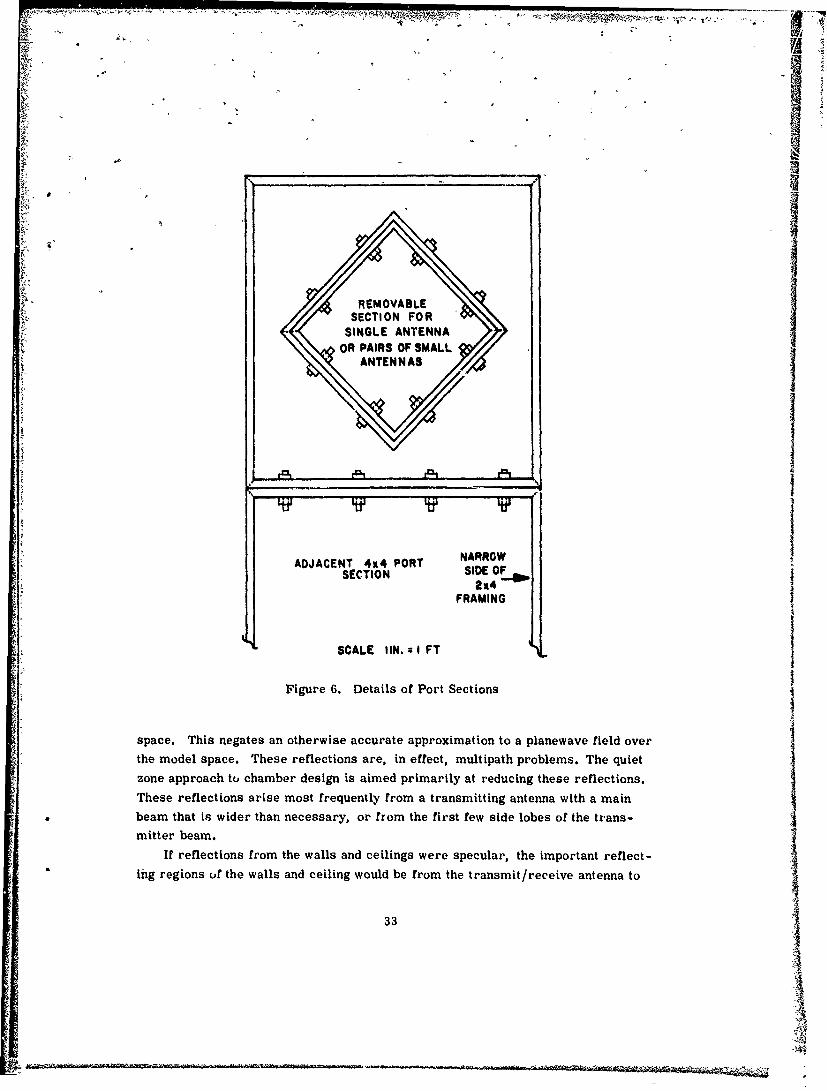
end. Details of the framing are shown in Figure 6. As suggested by Figure 6, the4 X 4 ft sections are large and may be inconvenient for smaller antennas. Hence,

smaller removable sections can be provided within these larger sections.

3.3 Chamber Reflectiomn

Serious reflections within a microwave anechoic chamber all originate fromthe transmitting antenna either through its main beam or side lobes. There are

three classes of serious reflections within a chamber. Each class introducessomewhat different errors and each class is susceptible to different cures.

The first class of reflections is comprised of energy reflected from the walls,

floor, and ceiling that passes through the space to be occupied by the model, the

model space. If these reflections are sufficiently strong so that the reflected

fields on the model space have an amplitude that is significant compared to the

amplitude of the direct radiation, an interference pattern is created over the model

31 "1

7N

I E---WIDTH OF WALL

HEIGHTOFWALL

Figure 5a. Port Arrangement of Full Wall Shielding. Dashedsection indicates optional additional port for access to RFequipment space for large equipment

I"WIDTH AT END-04

HEIGHT

Figure 5b. Port Arrangementfor Tapered Chamber

32

''' 4 Q

t REMOVABLE

i , SECTION FORr SINGLE ANT¢ENNA

OR PAIRS OF SMALL

SANTENNAS

NARROWADJACENT 4x4 PORT SIDROFSECTION SIDE OF, $

FRAMING

SCALE IIN. I FT

Figure 6. Details of Port Sections

space. This negates an otherwise accurate approximation to a planewave field over

the model space. These reflections are, in effect, multipath problems. The quiet

zone approach to chamber design is aimed primarily at reducing these reflections.

These reflections arise most frequently from a transmitting antenna with a main

beam that is wider than necessary, or from the first few side lobes of the trans-mitter beam.

In reflections from the walls and ceilings were specular, the important reflect-

Ing regions or the walls and ceiling would be from the transmit/receive antenna to

33

4

a point approximately midway of the chamber. This corresponds to incidence

angles at the walls from about 900 to an angle 0 given by:

0 = 57.3 tan 1 R/A (33)

where I is the total width of the room and R is the antenna to scatterer distance.Assuming as an illustrative example an effective finished room length of about

10 m with widths of 18 ft = 5.49 m yields

-=57.3 tan "1 10/5.49 = 61.20

Since scattering from the absorber-covered wall will be largely diffuse, important0Ireflections will occur out to perhaps 750.

A second class of reflections are potentially more serious for scatteringmeasurements. This class is comprised of those reflections that come from walls,

floor, and ceiling directly back to the receiving antenna. These reflections fre-quently are a significant part of the background signal that must be canceled in aCW system. the larger such reflections are, the more difficult it Is to maintaincancellation of the background signals during a measurement. The more serious

of these reflections occur through the far out side lobes of the antenna and there-

fore come from reflecting obstacles that are located physically close to the antennaso that little relief is provided by 1/R spatial attenuation. Since such reflections

may be a significant part of the background signal that must be canceled in CW

measurement systems, the structures giving rise to these reflections must beparticularly rigid and free from vibrations or other short term motions. Even

minute movements will upset low cancellation levels of the background signals

and thereby limit the measurement accuracy. It is to reduce the effects 'if suchreflections that tunnel antennas are highly recommended for radar scattering

measurements. The use of antenna tunnels readily reduce far out side lobes by15 to 20 dB and, therefore, the net sensitivity of a system to such reflections by30 dB to 40 dB. The reflectors used with reflector antennas for indoor scattering

measurements tend to be relatively small, accentuating spillover from conventional

feeds. An alternative antenna might be some form of the Bell horn if a proper

holding design could be found to permit ceitral axis feeding. The latter is very

useful because it permits ready rotation of the antenna for measurements at dif-ferent polarizations.

The third kind of serious chamber reflections come from the back wall, atwhich the transmit/receive antenna looks, and are due to two related causes, Thefirst is the obvious one which is that all of the transmitting beam that is not inter-

cepted by the scatter strikes the back wall and is reflected back toward the receiver.

34

This can alsq create a standing wave over the model space as well as provide asignificant contribution to the background signal. The best cure is to use high

quality absorber on the back wall,*The second source of backwall reflection error is a little more subtle. It is

due to forward scattering by the scatterer under investigation. The forward

scatter of an object is generally much larger than the backscatter, and this con-

centrated beam strikes the backwall directly in line with the transmit /receive

antenna and scattering model. For a sphere in the optics region of scattering, 5

for example

a (ka) 2(ira)2 (33a)~forward 2 '3a

"back - ( a2) (33b)

resulting in such forward to backscatter ratios as given in Table 4.

Table 4. Forward Scatter to Backscatter Ratios for a Sphere

! ar a118 °) .(ka) 2

r a(O°)

Sphere Size ar Sphere Size r(ka) (dB) (ka) (dB)

3.0 9.5 15.0 23.5

5.0 14.0 20.0 26.0

7.5 17.5 25.0 28.0

10.0 20.0 30.0 29.5

This edergy strikes the back wall and is partially reflected to the model whereit is again enhanced by forward scattering and returned to the transmit/receiveantenna, resulting in an error signal that can be relatively large under adverse

chamber arrangements and which is difficult to separate from the true signal that

is backscattered from the model.

*5. Van De Hulst, H. C. (1957) Light Scattering by Small Particles John Wiley& Sons, Inc., New York, Chapt. 9.

35

The following analysis of signal strength at the receiving antenna due to the

forward scattered signal is approximate, but provides a simple estimate of errorsfrom this source.

3.4 Reflnctions from Back Wall

Three distinct properties of reflections from the back wall can have serious

effects on measurements of scattered fields, and the three will be examined in-dividually in this section, The properties of concern are the amount of powerreflected to the receiving antenna with no scatter present, the field distortion

caused over the model space by backwall reflections, and the power returned tothe receiver from the back wall by way of forward scattering of the model.

3.4.1 POWER REFLECTED TO THE RECEIVER WITH

NO SCATTERER PRESENT

From Figure 7. the power density from the transmitter incidence on the back-

wall Is

P P : R2 )2 (power incident on back wall) (34a)

where Pt is the total transmitter power radiated by the antenna, Gt is the gain ofthe antenna, R1 is the distance from the transmit/receive antenna to the center ofthe space to be occupied by the model, and R2 is the distance from the center of

the model space to the backwall. Let the area of the backwall that is illuminatedby the incident beam be assumed to be elliptical. Then the axes of the ellipse aregiven by (HI + R2)MA and (R + R2 )0B where 0A and #B are the elevation and

azimuth heamwidths of the antenna. Generally. half power beam angles providesufficient accuracy but 1/10 beam angles may be used for better results. The area

of the wall that is illuminated is

(wall area illuminated) = 1. (R1 + )2 .AB 2 (34b)

Power reflected by the wall to the receiving antenna is

P Pt Gt (

rw (4)2(R + R2 )4 1 2 A#B w

Pt Gt (power density at transmit/2 OAB rw receive antenna from (34c)

16(42)(Rl + 1 2 ) back wall)

36

where r w Is the power reflection coefficient per unit area of the wall. The power

absorbed by the antenna is

Pt G2 X2

r 16(4s)2 (R 1 + R2)2 'AB (3

and

Pr G2 A2 (received power from back wall, (

F 16(4 1)2 (Ri + R 2) 2 'A Brw ' no scatterer) e

Note the i/R 2 behavior that is a direct consequence of the wall's acting as an

extended scatterer instead of a point scatterer.

Reflections of this kind from the back wall are one of the principal couplingmechanisms between the transmitting and receiving paths of a cw cancellation

scattering measurement systems, and the power described by Eq. (34e) is a

principal component of the background and leakage signal that must be canceled or

reduced. To obtain a feeling for the magnitudes involved in Eq. (34e) consider the

following example, namely a chamber with a total working length of (HI + R2)

10 m be used for measurements at 3 GHz () = 0. 1 m). Let the transmit/receive

antenna be circular and the largest one for which the conventional far field cri-

terion can be satisfied in the chamber. Thus,

/X (R1 +R 2)X

R1 +R2 2D2 /X 0 D= 1 2 ) - 0.707 m

Also, let the antenna be 60 percent efficient. As will be shown subsequently,G 0.3 12(H I + R2)/\. For simplicity, let the beamwidths be equal and given by0 A = OB X/D. Eq. (34e) becomes

Pr 0.9T4 (R1 + R2 )2X2 2

.- 16(4s)2(R1 + R22 (34f)

(0,31)2 - w (34g)

pr 10.3 1-- 9 )r

N? Pt \16 \ 5 w '~ w

37

If 40 dB absorber is used on the backwall, then Pr/Pt 6.94(108); for 20 dB

absorber the result is 6. 94(106). It is interesting to compare this result tothe

power returned by a sphere of ka 20 placed at R 8 m and also measured at

f = 3 GHz with the same antenna. Inserting the appropriate numbers in Eq. (32)yields Pr/Pt = 3.43(105). Hence, power received from the wall covered with

40 dB absorber would not contribute significant error to measurement of a ka = 20sphere with no additional cancellation; however, if 20 dB absorber were used at *

least 10 dB of cancellation would be required to insure no more than ±1 dB error

in the measured results.

3.4.2 FIELDS OVER THE MODEL SPACE, NO SCATTERER

The incident power density at the model space due to the direct wave from the

transmitting antenna is given by Eq. (34a) with (RI + R2 ) replaced by RI. The

power density due to reflections from the back wall is given by Eq. (34c) with

(RI + R 2 ) replaced by R2 . These fields are traveling in opposite directions and

produce an interference pattern over the model space with a standing wave ratio

(SWR) given by

Pt Gt + lt t 0A B "w

S'rR2 (34i)

FIR 24R 16(4w)R 2

or

SWRm _ 1/R 2) w (34j)1 - 1/4(R1 /R 2 ) B OA rw

where variations of 1/R 2 over the model space have been ignored and a subscript

on SWR is added to designate the model space. Equations (34j) and (34c) assume

the point where the power is to be determined to be in the far field of the illuminated

area of the wall. The most common situation occurs with the model space veryclose to the wall. For this case a more accurate model is obtained simply by ig-

noring the spherical spreading and assuming the wave from the wall to be reflected

to the model space simply as a planewave. In this case,

38

SWR •

=W I -..Lr (34k)m 1. *

In this case, if 40 dB absorber is used rw 10- 4 and w 10 "2 so that

SWRm = 1.01 17 dB. If 20.dB absorber were used, r w 10- 2 and

SWRm = 1. 222 = 1. 74 dB.

3.4.3 POWER AT RECEIVING ANTENNA DUE TO FORWARDSCATTERING BY MODEL

Let a scattering model be located in the model space at a distance RI from thetransmit/receive antenna, and a distance R2 from the wall (Figure 7). The power

density from the transmitter is given by Eq. (34a) with RI replacing (R1 + R2 ).

The power returned from the model directly to the receiving antenna is

(power density at antenna .t Gt aB (35a)from model backscatter) = (0)2 2

where aB designates backscatter cross section. The power density at the wall due

to forward scatter of the model is

(power density at wall PtGtOFdue to forward scatter) (4)2 2 (35b)

Again, since the model may be quite close to the wall and hence not in the far fieldof that patch of the wall that is illuminated by the forward scatter lobe of the mode,simple plane wave reflection is assumed, Hence, the power density at the modeldue to reflection of the forward scatter by the wall is

(power density at model Pt GtF (after reflection from wall) 2 2 2 (35c)(4 70 R RR2

This wave again undergoes forward scattering, this time toward the receivingantenna. The power density at the receiving antenna due to this source is

(power density at antenna F rv (3 5d)due to forward scattering) - 3 R4R2

39

- -1-- R - 04

SCATTERER

TRANSMIT/RECEIVE ANTENNA

BACK WALL

Figure 7. Geometry Illustrating Forward Scattering

The ratio Pr of this power density to the desired power density from the model

backacatter is

PtGt 2Frw (40)2Rl F

P r °r2 t toB B 4R 2

As an example, consider the scattering model to be a sphere of ka 20 located atR2 I m from the wall. From table 4, F = 400 a, and if the measurements areto be made at 3 GHz, B = l1 . Therefore,

-1600 a 1 r" 40. 53 r

For this example, 30 dB absorber would be sufficient to insure errors from thissource to be no larger than *1 dB. For a more general scatterer, that may have

higher ratios of aF to aB even 40 dB absorber may be marginal. The importance

of measuring the model at minimum values of R2 is clear from Eq. (35e). Also,

the desirability of using the best possible absorber near the center of the back wall

where illumination by forward scatter is strongest is clear.

Two methods of minimizing errors due to reflections from the wall are con-

tained in Eq. (35e). They are to reduce r and increase R2. An additional methodw 2that is also related to reducing Pw has been used with varying reported degrees of

success.

This method is to tilt the back wall so that the reflected energy misses themodel and antenna. In effect a null of the scattering pattern of the wall is directed

40

along the central axis of the experiment. In fact, the success of this method de-

pends on the" reflection from the back wall being largely specular instead of diffuse.The additional cost of including a tiltingwall will be substantial because a movable

i* wall must have an independent supporting structure that is absolutely rigid and

vibration free, and the wall must have a mechanism for precisely controlling itsmotion. Any. vibrations introduced by the wall will limit cancellation levels that

can be maintained and the reduced cancellation levels that can be maintained can

easily introduce error limitations that outweigh reduced back wall reflections.Also, the movable wall will not be useful for measurements that are to be madeover a program controlled set of frequencies.

A much cheaper alternative to the movable wall is to preserve the capabilityof measurements with the experimental axis skewed with respect to the longitudinalaxis of the chamber, this is, with the model placed to one side of the other of the

center of the chamber.

3.5 Estimated Interference from Multipath Signals

This section contains a zeroth order approximate estimate of the maximum

strength to be expected at the central axis of the chamber from signals that are"7 reflected from the walls, floor, and ceiling, and traverse the model space.

R The estimate can be made quite accurate by using bistatic scattering pattern

of the actual absorber chosen, and by using the actual antenna patterns at the fre-quency of interest; the basic technique will be the same as used herein.

The appropriate geometry is sketched in Figure 8 where R is the direct dis-tance from antenna to model, the wall-to-wall chamber width is w, the antennapattern angle is 6, and the angle at which offending rays strike the absorber is 0.

Because of Snell's Law, the most prominent offending reflections will always occurat points along the wall midway between the antenna and model, even when accountis taken of the actual diffuse nature of scattering by the absorber. For simplicity,

it is assumed that reflections take place from the base of the absorber.

SI (wn "i'IW/2 Il

I IW/2I I

I I lw/aI

Figure 8. Geometry for Estimating Multipath Reflections

41

If E is the maximum field just in front of the antenna, the direct held at the0

model space is

E /mo = Eo!R (36)

The reflected field at the model is approximately

s a o (7

Eml= RI

where a s is the ratio of the antenna field in direction to the field in the direction

of the main beam; a is the reflection coefficient of the absorber at angle 0; and

R 1 is twice the distance from the antenna to the point of reflection, the distance

traveled by the reflected ray. The ratio of the fields at the model is

ER Eml/Eo a aHsaa/1 / (38)

From Figure 8

R 1 - I + (w/R)2 (39)

(57.3 tan- 1 w/1lo (40)

0 90 - (57.3 tan- I /) (41)

Therefore

1 (42)' wR) 2

and

S 11E - sa (43)H 1 + (w/R) ": '

In dB

ERdB ' sdB+aadB 20 log + (w/) 2 (44)

42

where asdB is simply the value in dB of the antenna pattern at angle 4 and aadB is

the absorber reflection coefficient in dB at angle 0 = 900 -

The theoretical pattern of a circular antenna with uniform illumination is givenby Eq. (13). In dB,

as 20 logEc 20 log L rD/. sin . (45)

For convenience this function is graphed in Figure 9.

-10

-20I-30LL1

Figure 9. Theoretical Pattern-CircularAperture Uniform Illumination

In the worst case, reflections from both walls, the ceiling, and floor would

all arrive in phase at the model. In this case Eq. (43) is multiplied by 4 and Eq.(44) becomes

E RdB 12+ asdB + a dE 10 og(l+(w/R) (46)

43

As a function of R the worst case will occur when R is largest because this is whenthe angle 4 corresponds to the closer-in side lobes that are higher, and when the

angle of incidence on the absorber is furthest from normal.

For the following examples, R = 30 ft and w = 18 ft. The attenuator factorsare taken from the following section. With these values of R and w, for all of the

calculations,

* tan 1 18/30 310, sin = 0.5150

000=90 - = 59'

20 log 1 + -(w/R)2 =1. 34dB

Equation (46) is used for the examples.

Examples:

1. f= 1GHz, D=3ft

VD-- sin = 4.85 asdB =-19 dB, aadB -25 dB, ERdB -33.3 dB

2. f= 2GHz, D =3 ft, = 0.492 ft

-- sin =9.86 asdB =-28dB, ad -42dB, E =-51.3 dB

3. f =4GHz, D= 1.5ft, = 0.246 ft

Dsin= 9.86 asdB -28 dB, aadB = -42 dB, ERdB -59.3 dB

4. = 10GHz, D= 1.0ft, A= 0.0983 ft

sin 16.46 asdB -35 dB, aadB -48 dB, ERdB -72.3 dB

Even under conditiuns of relatively diffuse scattering from the absorber thereshould be combinations of R for which 0 is at the antenna pattern nulls and for

which ERdB is very low. This may be an especially important consideration for *

obtaining high quality results with relatively large, low cross section scatterers

at frequencies near 1 GHz.

4

44

3.6 Absorber Characterstig

If the use of sophisticated chamber design for scattering measurement systemsis ruled out by arguments of versatility, the remaining questions center on thechoice of absorber to be used to line the floor, ceiling, and walls of the chamber.To provide a basis for these choices the characteristics of current state of the art

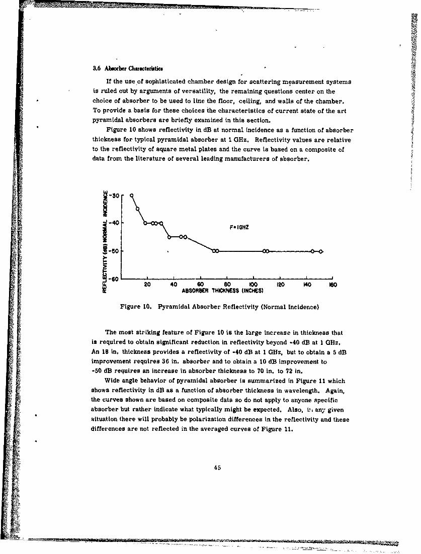
pyramidal absorbers are briefly examined in this section.Figure 10 shows reflectivity in dB at normal incidence as a function of absorber

thickness for typical pyramidal absorber at 1 GHz. Reflectivity values are relativeto the reflectivity of square metal plates and the curve is based on a composite of

data from the literature of several leading manufacturers of absorber.

350

5K -40F IOHZ

5 -

F Igr (NorI , Inciece

20 40 60 80 1O0 120 140 160ABSORBER THICKNESS (INCHES)

Figure 10. Pyramidal Absorber Reflectivity (Normal Incidence)

The most striking feature of Figure 10 Is the large Increase in thickness that

is required to obtain significant reduction In reflectivity beyond -40 dB at 1 GHz.An 18 In. thickness provides a reflectivity of -40 dB at 1 GHz, but to obtain a 5 dBimprovement requires 36 in. absorber and to obtain a 10 dB improvement to-50 dB requires an increase in absorber thickness to 70 in. to 72 in.

Wide angle behavior of pyramidal absorber is summarized in Figure 11 whichshows reflectivity in dB as a function of absorber thickness in wavelength. Again,the curves shown are based on composite data so do not apply to anyone specificabsorber but rather indicate what typically might be expected. Also, I-, any givensituation there will probably be polarization differences in the reflectivity and these

differences are not reflected in the averaged curves of Figure 11.

45

. . .+ . + . + . + , . . . . . . . . , . . + . . .

L. .... .. + .+ + + +

-10

-20 - INCIDENCE ANGLE(DEG FROM NORMAL)

-- 30

.- 50

-60

o-

o ~q 0QQ QO OQOq

ABSORBER THICKNESS IN WAVELENGTHS

Figure 11. Wideangle Reflectivity-Pyramidal Absorber

As might be expected the greatest deterioration in reflectivity with angle occursat lower frequencies for a given absorber thickness. Thus, the reflectivity at

1. 0 GHz with 18 in. absorber changes from -40 dB at normal incidence to about

-16 dB at 700 incidence.

As shown previously, serious reflections from walls and floors in a chamberof about 10 m length and 6 m width would occur at angles of incidence to about 600and allowing for diffuse reflections, to about 700. Based on Figure 11, the use of24 in. absorber on the walls, ceiling, and floor would insure reflectivity no higherthan -30 dB for frequencies of higher than approximately 3.0 GHz, and reflectivity

of -40 dB or better for frequencies higher than approximately 7.4 GHz.

For convenience, reflection coefficients for 18, 24, and 36 in. absorber atincident angles of 00, 500, 600, and 700, for 1. 0 GHz are summarized in Table 5and typical values at normal incidences for a range of frequencies are summarized

in Table 6.

46

Table 5. Approximate Pyramidal Absorber ReflectionCoefficients at 1 GHz

Reflection CoefficientsIncidence (in dB)

Angle 18 in. 24 in. 36 in.

V00° (normal) -40 -40 -45

500 -25 -30 -40

600 -22 -25 -30

700 -15 -18 -22

At higher frequencies where a given absorber contains more wavelengths, reflec-tion coefficients remain good out to even 700. At X-band where the wavelength is

approximately an Inch, the reflection coefficient would be approximately -40 dB at070.

Table 6. Normal Incidence Frequency Behavior, Pyramidal Absorber

AbsorberThickness Frequency Band (dB)

(in.) K KU X C S L

18 -50 -50 -50 -50 -45 -40

24 -50 -50 -50 -50 -50 -40

36 -50 -50 -50 -50 -50 -45

There are several additional basic considerations in absorber choices. Thefirst is that use of thick absorber with improved reflectivity levels also reduces

the usable measurement space in a chamber of finite size. and by moving the wallscloser to the scatter, the advantages of path length attenuation are reduced. Theend result can well be no better han having a thinner absorber placed further fromthe scatterer.

The second consideration is that significant improvement in wide angle reflec-

tivity might be achieved by mounting the absorber at 45° angles to the horizontal orvertical. That is, instead of aligning the standard 2 X 2 ft sections with their edgesparallel to the walls and floor as is common practice, align them at 450 to these

47

7777,.

surfaces. When radiation from the antenna falls on the pyramids from other thannormal incidence, the energy tends to strike the flat surface of the pyramids in the

usual mounting configuration. These flat surfaces are noe particularly goodabsorbers and multiple absorbing reflections are discouraged with this orientation

of the absorber. If the absorber iS mounted at 450 orientation, energy incident at

wide angles will tend to strike the corners of the pyramids and be absorbed byadditional multiple reflections between the pyramids.

444. TRANSMIT/RECEIVE ANTENNAS

The gain of a reflector type of antenna is given by4 (Chap. 7)

4rAe

G e (47)

where Ae is the effective area of the reflector and X is the wavelength. Typically,reflector antennas are about 60 percent efficient because of spillover from the

feeds and power tapers across the apertures to Improve side lobes. Assuming

60 percent efficiency,

4(0. 6)A (48)

where A Is the physical area of the reflector. For a circular reflector of diameterD,

wD2

A - (49)

and the gain becomes

G = 0. 6w2 (D/ )2 (circular antenna 60 percent efficient) (50)

The antenna far field is given by the same relation as the conventional scattering

far field,

R =2D/x (51)

Based on the conventional far field criterion, the largest antenna that can be uti-lized over a range R is, from E4 . (51)

48

D . (52)

Inserting this value of D into Eq. (50) yields

G = 0.3f 2 (R/X) . (53)

The point is that if the antenna must be a distance R from a scattering model

to measure in the far field of the model, the largest antenna that can be used,

subject to the usual far field criterion, is given by Eq. (52) and has a gain given by

Eq. (53) or Eq. (50).

Since the far field criterion of the antenna and the scatterer are the same, it

follows that the antenna defined by Eq. (52) is equal in size to the scattering model.

An antenna equal in size to the scattering model is also an optimum antenna to

be used for scattering measurements under conventional far field criteria. The

reason is that f a larger antenna were chosen, R must be increased beyond the

minimum required by the model and the received power. Eq. (25), will be reduced4by a factor of k where the far field distance, R, required by the larger antenna is

given R- kR. If a smaller antenna is used, the receiver power will be reduced

through the G' term by a factor of k2 where the smaller antenna is related to the

optimum only by DI = kD because R in this case is determined by the model and

cannot be reduced by use of the smaller antenna. The optimum antenna, equal in

size to the scattercr, in effect minim'zes R, the most sensitive term in the power

relation.

Equation (19) shows that for a uniformly illuminated circular reflector antenna

having a diameter D equal to the maximum model dimension L, the lateral distance

between half power points of the beam in I = 2 L, twice the model's maximum

dimension. With the aid of Eq. (15) it is easy to show that for a model perfectlyxcentered in the antenna beam so that it extends between I = ±i: where x = uDO/X,

the incident field will be down by -0. 71 dB at the ends of the model for a total

variation over the model of ±0.35 dB.

An expanded graph showing the first 3 dB region of the pattern of the uniformly

illuminated aperture of Figure 9 is shown in Figure 12 to illustrate the field varia-

tion to be expected in the central region of the beam. In effect, Figure 12 defines

Zthe accuracy with which a model must be located within the beam. For example,

for a variation no greater than ±1/2 dB of field over the model space, the model

must be included in a region of approximately ±0.6 D of the center of the beam.

Similarly, for the field to be constant within ±1 dB, the model must be within

*0.84 D of the beam center.

49

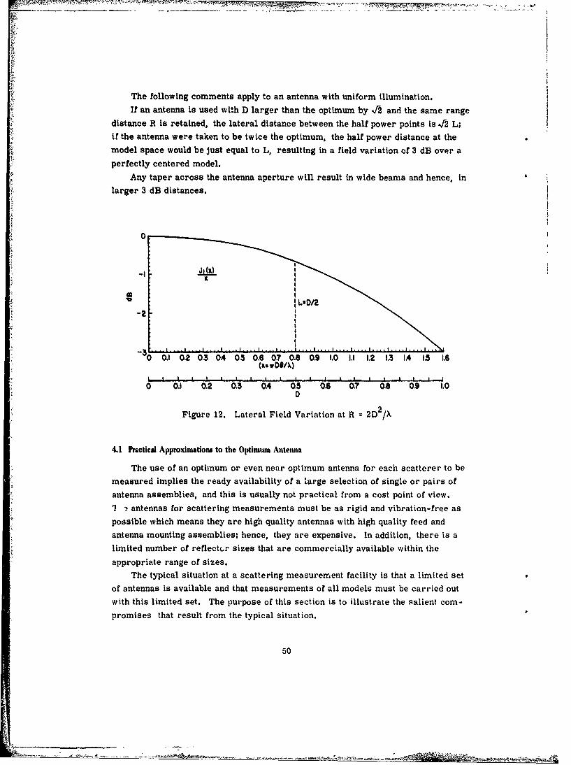
The following comments apply to an antenna with uniform illumination.If an antenna is used with D larger than the optimum by %/2 and the same range

distance R is retained, the lateral distance between the half power points is 2 L;if the antenna were taken to be twice the optimum, the half power distance at themodel space would be just equal to L, resulting in a field variation of 3 dB over aperfectly centered model.

Any taper across the antenna aperture will result in wide beams and hence, inlarger 3 dB distances.

; -I

o 0.1 0.2 03 04 0.5 0.6 07? O. 0.9 1.0 1.1 1.2 1.3 1.4 IA 1.6(x, vDt/))p I I p p p p p p p p p p I P P I

0 0.1 0.2 0.3 0.4 0.5 0. 0.? 0.8 09 1,00

Figure 12. Lateral Field Variation at R 2D2/X

4.1 Prmctical Approximations to the Optimum Antenna

The use of an optimum or even near optimum antenna for each scatterer to bemeasured implies the ready availability of a large selection of single or pairs ofantenna assemblies, and this is usually not practical from a cost point of view.

'I '! antennas for scattering measurements must be as rigid and vibration-free as

possible which means they are high quality antennas with high quality feed andantenna mounting assemblies; hence, they are expensive. In addition, there is a

limited number of reflectr sizes that are commercially available within the

appropriate range of sizes.The typical situation at a scattering measurement facility is that a limited set

of antennas is available and that measurements of all models must be carried out

with this limited set. The purpose of this section is to illustrate the salient com-promises that result from the typical situation.

50

Consider a facility operating from 1 GHz to,40 GHz with a chamber having amaximum usable range of R = 32 ft and focus attention on maximum model sizes

that can be handled. Let the optimum antenna be approximated by three sets of

reflector antennas having diameters of 36, 18, and 12 in. respectively. These

three antenna approximation to the Ideal is shown in Figure 13 over the 1 to 40 GHz

frequency band. Note that the curve for the optimum antenna of Figure 13 is also

the curve for the largest model that canbe used with a variation of no more than

*0.35 dB In the Incident field over the model.The principal question is how the use of a limited set of antennas of fixed size

affects the lateral working distance at the model space, in this example, at a meas-

urement distance of R = 32 ft. Assuming circular apertures with uniform illumina-tion, half power beamwldths are given by Eq. (19a) which becomes

I - R/(fD) (54a)

with lengths and distances in ft and frequency f in GHz. For the present example

I = 32/(fm) . (54b)

For the optimum antenna I = 2 D as shown by Eq. (19b).Lateral half power distances calculated from Eq. (54b) for the three antennas

of 36, 18, and 12 in., diameters and for the optimum antenna are shown in Fig-

ure 14.

In general it is advantageous to choose matched antenna and feed sets so thatthe feeds for various frequency ranges can be easily used in any of the reflectors.

Thus, for example, the smaller antennas are useful at lower frequencies forsmaller scattering models that can be measured at shorter ranges. Again it is

emphasized that the antenna reflector, the feed, and the mounting arrangementshould be absolutely rigid and vibration free. Although the above discussion hasbeen in terms of reflector antennas, lens antenna, and horn lens combinations are

also very useful for scattering measurements. The results as outlined generallyapply to these types as well. Once specific antennas have been chosen the actual

beamwidths of the chosen antennas can be utilized to construct a graph such as

Figure 14.A properly designed set of reflectors and feeds offers the possibility of varying

the focus, and this feature can sometimes be quite useful. For example, defocusing

will result in a wider beam and hence a larger region with less field variatio1 overthe model space. Similarly, for small models with low cross sections, focusing

the larger antennas at short measuring ranges in their near fields can sometimes

be advantageous by increasing the field concentration over the model space.

51

I

4.0 l IIIII I

36 INCH ANTENNA3.0

PTIMUM ANTENNA V(F, R /2) 7-

2.0I8 INCH ANTENNA

1.0 R a 2 T 12 INCH ANTENIA - - - - - -

01 12.0 118.0 26.01.0 2.0 3.0 4.0506.0 8.0 100 15.0 20.0 30 40

F(GHZ)

Figure 13. Three Antenna Approximation to Optimum

9

36ISINCHHDISH

41 OPTIMUM

4

3

2

I Rv32FT

01.0 aO 30 4050 60 10 100 150 20 30 40F(GH.Z)

Figure 14. Half Power Distances at Model Space forThree Antenna Approximation to Optimum (UniformIllumination, Ri 32 ft)

52

4.2 Tunnel Antennas

Significant improvement in the performance of all of the smaller antennas can

be achieved by fitting them with tunnels, and it is recommended that this be done.

The tunnels should be electromagnetically sealed at the rear, either to the rim or

rear of the reflector or, in case of centrally fed antennas, to the waveguide feed.

The principal effect of the tunnel is to reduce spillover. Thus, the use of a tunnel

significantly improves ability to maintain background cancellation. The reason is

that the spillover energy corresponds to far out side lobes in the far field antenna

pattern. These far out side lobes extend to 900 and frequently further from the

main beam direction. When the antenna is used for scattering measurements, thisenergy in the far out directions strikes nearby objects and is at best partially re-

flected back to the antenna. Since these reflecting objects are nearby, the 1/Rlosses are small compared to those from the scatterer under investigation. The

antenna Is therefore tightly coupled to these nearby objects through its far out side

lobes and the slightest movement of these scatterers relative to the antenna destroysthe background cancellation. Reduction of the far out side lobes reduces the im-

portance of nearby reflections to the balance.

A cheap method of constructing antenna tunnels for small round antennas con-sists of using thin absorber of the AN/75 family and purchasing sections of chimneyor vent pipe equal in diameter to the reflector diameter plus twice the absorberthickness. The absorber and reflector are then fitted inside the pipe. The reflec-

tor can be held in place by screws or longer bolts passing through the pipe and therim of the reflector. The pipe can be sealed at the rear with heavy duty aluminumfoil and conducting aluminum tape. Interior supports for the aluminum toil, or a

metal cover that is stiffer than the aluminum foil is recommended. The distancethat the tunnel extends beyond the antenna face depends on the diameter of the

antenna and the particular absorber that is used, and is best determined experi-mentally because the actual extension chosen usually represents a compromisebetween reduction of the far out radiation and slight decreases of gain and slightbeam broadening that also occur. Typical useful extensions have been found to beapproximately 7 to 8 in. for a 12 in. dish diameter and 4 to 5 in. for a 6 in. dish

diameter at 10 GHz.Typical results of using a tunnel of the type described above with a 6 in. dish

and double dipole feed at 10 GHz are shown in Figure 15 for the tunnel extending

about 4 in. beyond the reflector face. For the H-Plane patterns that are shown,this extension results in approximately a I dB loss of gain and an increase of

approximately 25 percent in the 3 dB beamwidth but significantly reduces all rad-

iation at angles greater than approximately :k600 from the main beam.

53

t t-10 -

20

II\NOTUNNEL

-J,le,', 1 rW %I

6 INCH, DOUBLE DIPOLEFEED

H, PLANE PATTERNF a 10 0HZ

I I I I I I00' 144 108" 720 36' 0' 36' ?2" lOS' 144' IO0 216"

AZIMUTH ANGLE (DEG)

Figure 15. Results of Using Tunnel to Reduce Far Out Radiation (H-planepattern, 6 in. reflector with double dipole feed, f = 10 GHz)

5. MODEL SUPPORT STRUCTURES

The model support structure consists of three parts: the mount, the polyroam

column, and the mounting saddle. Model supports other than polyfoam columns

are used, 6 particularly for very heavy or very small models, but polyfoam columns

are so common and convenient that the present discussion will be confined to them.

A typical model support structure as it might be used for radar scattering meas-

urements is shown in Figure 16.

In order to accommodate a wide variety of model sizes and weights conveniently

as well as experiments at widely differing frequencies, a multisection column with

interchangeable sections is suggested by Figure Ila. For example, a 4 ft model

for I GHz measurements might easily weight 100 lb and require measurement at

the chamber center height of 9 to 11 ft, whereas a 4 in. model for measurement

at 10 GHz to 40 GHz is more likely to weigh less than I lb and be more conveniently

6. Freeny, C. C. (1966) Target support parameters associated with radar reflec-tivity measurements, Proc. IEEE 53:929-936.

54

MAIN BEAM REMOVABLE

a-MODEL SUPPORTS/0 .SECTION

l4l (POLYFOAM)

REPLACEABLE- CIRCULAR

CYLINDRICAL SECTION(POLYFOAM)

lOFT MOUNT ASE

BASE SHIELD - BASE/ u,"-TRUNCATED CONEI \(POLYFOAM)

/ /\METAL ORWOOD PLATE

U LBASEELYMOUNT&I I SELYSL

Figure 16. Typical Model Support Structure

measured at a height of 4 to 5 ft. In addition, flat surfaces of polyfoam must bekept to a minimum in the immediate vicinity of the model for reasons to be dis-cussed shortly. The sectional column approach permits measurements at allfrequencies to benefit from the relatively large investment that is required for aprecision mount and its controls. If measurements are anticipated involving veryheavy models as well as small ones, the additional cost of acquiring two mounts ofdifferent size and capability will usually be rapidly recovered in convenience thatleads to reduced measurement times. The average reduction in time per measure-ment may be only 2 to 3 min, but it typically involves at least two people and isrepeated many times each year so that the cost saving rapidly multiplies.

Sections of the polyfoam column can generally be fitted together by turningthe cavity and extensions of adjoining sections in a lathe. The fit must be goodand it is a high wear connection but changes are not made very frequently.

The overriding requirement of the entire model support structure is that it befree of random wobbles if the system is to be used for measurements of phase. At10 GHz, for example, the wavelength is 1. 18 in. and one degree of phase corre-sponds to 1.18/360 = 0.0033 in. While a random wobble of :*1/16 in. will have nomeasurable effect on power or amplitude measurements at 10 GHz, it would intro-duce an error of *2 (0.0625/0.0033) = :*380 in measurements of phase. The factorof 2 is introduced because of the two way path. At 40 GHz, the phase error intro-duced by a 1/16 in. wobble is four times as great or :1:1520.

55

5.1 The Mount

The principal requirements of the mount are (1) that it be capable of handlingthe heaviest models to be measured, (2) that it be capable of precision control ofat least 0. 1 in azimuth, (3) that it be fitted with wheels or castors for easy move-ments in at least two orthogonal directions, (4) that it be rock steady when lockedin position, and (5) that it be compatible with control and data processing equipment

that will be used. A number of commercially available antenna testing mounts ful-fill these accuracy requirements and are available in a wide range of sizes. Inaddition they are designed to interface with a wide assortment of data handlingequipment from traditional analog pattern recorders to sophisticated computersthat provide both programmed control of the mount motion and programmed realtime manipulation of the data. Generally, the more automated mounts are mostcost effective when a large number of basically repetitive measurements are antic-ipated.

The precision rotation capability is required for measurements at high fre-quencies and measurements of phase. Consider, for example, the measurementof a 1 ft scatterer at 40 GHz. The scatterer will be essentially uniformily illum-inated. If the scatterer is a circular metal disk the half power beamwidth of itsprincipal backscatter lobe will be given approximately by 1/2 of the beamwidth ofa circular antenna with uniform illumination, Eq. (14b). With f = 40 GHz, X =X = 0. 295 In., and /1/2 0.72. This is the totE) angle between half powerbeamwidths of the principal backscattered lob. Clearly, a mount with azimuthcontrol accuracy of 0. 10 is barely adequate for such measurements. The phasetends to be relatively constant across principal lobes but to change rapidly near theedges of the beam. If the phase is to be sensibly tracked at all through these re-gions the mount accuracy must be at least 0. 10.

5.2 Buics of Polyfoam Columns

Columns of foamed polystyrene are the most widely used supports for scatter-ing models of up to a few hundred pounds in weight. Foamed polystyrene has avery low relative dielectric constant ranging from about 1. 02 to 1. 10 therefore lowbackscattering, although as will be shown, the backscatter is by no meansnegligible.

If experiments are centered vertically in the chamber, the required columnsupports could easily be as much as 7 ft long to extend from the top of the mount

to the vertical center of the chamber less half the models vertical thickness sothat the model is centered in the antenna beam. In addition, columns of severaldifferent thicknesses would be convenient to accommodate both large and smallmodels. Unless a completely new column is to be used for each different model,

56

a section of about 1 ft in height should be replaceable because the top of the column

will generally require special shaping to hold each different model.

Thin foamed polystyrene columns tend to bend even under their own weight if

they are more than 18 to 24 in. in length. Therefore, the complete column might

be fabricated in sections to permit a sturdy low cross section base and use of a

thinner upper section for small models. Several designs are possible of which a

typical one is shown in Figure 16. Ultimately, having several columns that can be

Interchanged on the mount base for different classes of measurements will prove

to be very convenient.

The foamed material generally comes in blocks and the columns must be cut

and turned from the blocks and planks. Procedures have included rough cutting

with a saw and final turning on a lathe with sandpaper as the cutter, and cutting with

a hot wire saw. The material generally dulls regular lathe cutting tools too rapidly

to make their use practical. Also, the columns tend to bend away from the force

of a cutting tool.

The columns must be absolutely circularly symmetric and mounted in the cen-

ter of rotation of the mount. One method of achieving centering of a smaller column

has been a series of guy strings attached to the column and a broad mount base at

1200 angular Intervals, The reason for the required centering care is that even

through backscatter from the column is small, it eventually becomes the dominant

term in the background signal as other sources of background scattering are can-

celed. Any forward or backward motion of the column as it revolves through a

pattern can disturb seriously the cancellation level. A digital cancellation scheme

that subtracts the background signal from the target signal might reduce these

tolerances and would be feasible if the facility were equipped for storing the signal

phase and amplitude on tape for later computer processing, or if the facility were

equipped for real time data manipulation with sufficient storage.

In so far as practical it is recommended that experiments be centered vertically

below the vertical center of the chamber if vertical centering requires a ladder or

steps to reach to model. This might be practical at frequency bands from about

8 GHz to 12 GHz and higher. The lower centering of the experiment simplifies

fabrication of the column and significantly reduces the physical effort of placing the

model on the mount and removing it from the mount, if the experiment permits the

model change without the use of steps. In the course of a good day of data taking

the process of placing the model on the mount, removing it, placing a reference

scatterer on the mount, may be repeated several hundred times and climbing even

three or four steps to reach the top of the mount each time is very tiring by the

end of the day.

57

5.2. 1 COLUMN DIAMETER VS MODEL WEIGHT

A conservative relation that defines the diameter of a polyfoam column of

height h to support a weight W is 7

d = 8(h/w)1/2(W/1E)1/ 4 (54)

where E is the elastic modulus and a factor of 2 has been added for safety. A con-

servative value of tl'e elastic modulus for styrofoam is 1500 psi.

As an example, W = 25 1b, h = 8 ft

d = 8(96/W)1/2 ( 25 5-I1/4 11,9 In.

5.2.2 BACKSCATTER-CYLINDRICAL COLUMN

The following argument is very approximate but it is simple and works quite

well. Polyfoam has very low losses. Therefore a plane wave incident on a column

of polyfoam is reflected from both the front and back surfaces and the reflections

are about equal in amplitude but the reflection from the back surface has a phase

lag approximately equal to the total electrical path through the material. Assume

the front and back surfaces to be planar. Then8

o(o) I kdh 2 I-j ej2kd, 12 IR(o) 12

where d is the column diameter, h is the length, and R is the reflection coefficient

for planar surfaces at normal incidence,

R = 1 " "/4(c - 1) (56)

sincej A 1 and (e - 1) << 1.

kdh2 2(7Q(o) = kd(2 - 1)2 (1 + 2 sin [2kd./r} . (57)

7. Knott, E. F. and Senior, T. B. A. (1964) Studies of Scattering by Cellular PlasticMaterials, Report No. 5849 -1 -F. Tfe Radiation Laboratory, Univ. of Mich.,Ann Arbor, Mich.

8. Senior, T. B. A., Plonus, M. A., and Knott, E. F. (1964) Designing foamedplastic target supports, Microwaves, 38-43.

58

Note that Eq. (57) has a maximum of

lh (C 1)2

'max 8 )2 (58)

when

2kdl= (4n + 1) ?/2 (59)

max 3O. 3(4n + 1); fmax (60)

8d%

where fmax is the frequency in GHz corresponding to a maximum, and d is the

column diameter in meters.

Equation (57) also has a minimum of zero when

2kd.,/c = (4n - 1) 1/2 (61)

or

-0.n 3n -1)mIn d.l (62)

Typical amax for columns are given in the following examples:

h = 8 ft, e = 1.05, d = 14 in. 2I,max = 10.39 GHz, armax = 0. 14 m2 = -8.42 dBSM

with the same column but lower dielectric = 1. 02,

,max = 10.55 GHz, amax 11. 8 dBSM

The most significant point from Eqs. (57), (60), and (62), is that the column can

be tuned to yield a minimum backscatter cross section at an infinite set of fre-

quencies, and at higher frequencies successive values of 'mi are reasonably close

together. Several of the adjacent minima of the preceding example, for example,

are (from Eq. (62))

fmn= 8.73, 9.36, 9.57, 9.99, 10.41. 10.83 GHz'min

59

/

I.

Although Eq. (57) was derived for normal incidence, it holds approximately

over a small angular interval near normai-so that it generally applies to all of the

column that is within the antenna beam.

The values of fmin' calculated or measured, are those values at which back-

scatter contributions from the column will be an insignificant part of the total

background signal.

5.2.3 BACKSCATTER-TRUNCATED CONE COLUMN

For heavier models, the truncated cone is very useful form of column. It is

also a useful column form for the bottom portion of a sectional column. The ques-

tion becomes what cone angle to choose. A very approximate analysis yields sim-

ple and useful results. If the backscatter from the finite cylinder is considered

not more than (for example) 300 from normal, the backscatter can be represented

reasonably in product form. That is, the broadside backscatter of the column is

multiplied by a pattern factor. Using the worst case of a broadside maximun,

Eq. (58), and the standard column scattering factor

0() -kdh (C-_ 1)2 sin (kh sin 0)2 (63)8 - (kh sin ) J

This function has zeros, or minimum in practice, when

0 -snl[I .2 (64)

Thus, in addition to tuning its thickness, backscatter from the column could be

reduced by tilting the column. Tilting the column is not practical but the next best

thing is to tilt the forward surface that is in immediate contact with the wave.

Doing this over 3600 leads to the truncated cone. Scattering from the sido of the

cone can be further reduced by serrating the sides of the cone.

5.2.4 FORWARD SCATTERING FROM POLYFOAM COLUMNS

Although polyfoam has very low relative dielectric constants at microwave

frequencies and low backscatter, the specular forward scattering near grazing

incidence is very large, a condition frequently overlooked in the use of polyfoam

as supports both in antenna experiments and in scattering experiments. The

result is that often more polyfoam is better than less.

Consider the Fresnel reflection formulas for a plane surface. Let 0. be theI

angle of incidence measured from normal, and assume perfect dielectrics. Then,

see Kerr, Chapt. 43

60

1!I

I I

ER = c os i - JC/C sin

-E =r l (65b)

C2 cos 0i + 4C 2 /c- sin 2 i

Let medium 1 be air and medium 2 be polyfoam. Let 0 - 900, grazing incidence.

Then

r - . (65c)

Note that Eq. (65c) is independent of E and, therefore, at these grazing angles, the

polyfoam might just as well be a sheet of metal (in at least one polarization). Also

note that Eq. (65c) extends over a small range of angles near 900.

From a practical view for scattering measurements, Eq. (65c) means two

things. The first is more bad news about reflections from the back wail. The

second is that a flat surface of polyfoam of even a few square inches should never

be permitted near the scattering model if there is any possibility of forward scat-

tering at grazing incidence falling on the model. Worst case examples include

conespheres, ogives, prolate spheroids, or even spheres placed on flat column

tops or slightly buried in flat sheets of polyfoam. The interfering results are

easily measured at X-Band with spheres below ka's of about I to 2 where measured

cross sections vary by I to 2 dB depending where the sphere is placed on columns

having top diameters of 4 to 5 in.

The preceding discussion has been carried out in terms of polyfoam but all

materials have a similar behavior. An absorber, for example, is commonly usedto prevent reflections from the metal parts of the mount base as shown in Figure 16.The absorber is typically mounted on a thick plywood base that is fitted with legs

to facilitate adjustments. In situations where the model is mounted only 4 to 5 ft

above the floor or where the model has supporting structural pieces that must beshielded from the incident field, particular care must be exercised to insure that

flat surfaces of the absorber pyramids do not forward scatter onto the model space.

This is a siutation where even a crude probing of the field with the shield in place

can pay high dividends by resolving mysteries of variations in the measured data.

Figure 17 shows the results of such a field probing when a shield of 18 in.

pyramidal absorber was placed about 2 in. below the column top where a small

61

A

12.0

)11.0

9.0

8.0

6.- -

4.0

H-PLANE 0-4-43.0- H-PLANE • "0

F'I0 GHZSCATTERERa 5/S1N. SPHERE

2.0-

1.0-

o q o ? oo qo

do

Figure 17. Variation of Power Over Model Space Dueto Forward Scatter from Absorber Shield

model was to be located for measurement. The objective was to cover a small

motor that was used to vibrate the model. The measurement frequency was 10 GHz

and the scattering probe was a 5/8 in. diameter metal sphere. The sphere was

suspended on a thin monofilament fishing line that in turn was hung over a polyfoam

block setting atop the column. Half-inch spaces were marked in black crayon on

the line and a corner of the polyfoam block was used as a position reference. With-

out the shield in place there was essentially no variation in the field over the region

that was measured. As can be seen from Figure 17, the presence ofThe shield

caused vat iations of as much as 8 dB even at distances of 8 in. or more above the

shield.62

'Miz

6. RF POWER SOURCFS

The principal requirements of an rf power source for a CW scattering meas-

urement facility are that (1) it cover the correct frequency range, (2) it producesufficient power, and (3) it have sufficient frequency stability and a sufficiently

pure spectrum to permit useful cancellation levels to be maintained over the meas-

urement times. In addition to the above, there are many applications for which an

automated capability is advantageous and this imposes an additional requirement

that the power source be compatible with the control equipment and other equipment

with which it must interface.The power requirements for a given set of measurements are easily determined

from Eqs. (25), (28), or (32). The frequency stability requirements are not soeasily stated, but the basis can be found from examining the CW cancellation proc-ess.

6.1 Cancellation Requirements

Let two signals that have traveled over different paths and through different

components but that originate from the same source be brought together at the

junction of a hydrid tee and their difference be observed in the difference arm of

the tee. In general, each path has a different number of wavelengths and compo-

nents whose rate of change of phase and attenuation with frequency differ for even

small changes in frequency.Let the two signals be represented as

eA = A cos (tot +

eB = B cos (wt + 0B ) (66)

where A and B designate, respectively, the two different paths. The net difference

signal is€

e --A cos (wt + A) -B cos (tot + OB) 167a)

= A [cos (tot + A)- B/A cos (wt + 4B) . (67b)

Let the amplitude of the B-path signal be adjusted so that it differs from A byonly a small amount L. Then

B- A + (68a)A

63]

and

[cos (t + OA) -cos (Wt + OB) - cos (t + OB)] (68b)

-[2 sin 1/2 M2,t si+ n 1/2 ~ B o w B].(68c)

For e to remain below some desired level over a measurement time, the difference

(A ) and the ratio.X must remain less than levels determined by Eq. (68c)for the measurement times. The maximum value of the coefficient of each is 1.Using this maximum or worstcase value and small angle approximations.

ed 20 log1 ~ 20 log I( B ~ ~(69)

To illustrate the magnitudes Involved In Eq. (69) consider the following examples.

For simplicity, first consider A 0. Then If it is desired that edB remain below-100 dB over a measurement time, the phase difference ( must remain

less than 0.00001 radian or 0.000580 over this time period. Similarly for edB toremain less than -80 dB. #A " ) must remain less than 0.0001 radian or

0.0058°. (If = 0, for a cancellation level of -100 dB L must be less than

10- 5 and for a cancellation level of -80 dB A must remain less than 10 " .

6.2 Frequency Stability Requirements

In a typical CW cancellation system the components of background signal coverthe complete range between two extremes. On the one hand, there are directly

coupled signals of relatively high amplitude but having a path length nearly equal to

the path length of the signal used for cancellation. On the other hand, there are

signals of much lower amplitude but that have traveled to the back wall and backand therefore have path lengths much greater than that of the canceling signal. Forthe latter components, long line effects increase frequency stability requirements

as will be shown.The fundamental concern with frequency stability is that it be sufficiently good

that it is not the limiting factor in achieving and maintaining cancellation levels.

The following discussion is aimed at cancellation at rf. Let two signals bederived from the same transmitter at a directional coupler. A subscript A denotes

the signal that has traveled through the transmission path and OA designates thetotal phase of this signal from the separation point. Similarly. a subscript B

designates the reference cancellation signal that travels over a controlled path athrough an attenuator and phase shifter that introduces an adjustable "trimming'

64

ARO

phase OC" The total phase of signal B except that introduced by the phase shifter

is OB"

At the difference terminal of a hybrid the net signal is

6A =Acos(w t+OA) , =Bco s (wt + 3 + C ) (70a)

e =A cos (wt+OA) -Bcos (wt(+B + C ) " (70b)

Adjust the attenuator so that B = A. Then

e = A (cos (wt + OA) - cos (wt + 0B + OC) ] (70c)

= 2A sin 1/2 (wt + OA + OB + OC) sin 1/2 (OA "13 C) (70d)

Clearly, e = o when

OA -B - OC = 2nrt (70e)

The phase terms are

fwX = 21 f (7lb)

OB =' :7- c (b

where for simplicity an "adjusted" length X has been introduced to represent the

free space path plus an adjusted path through transmission lines so that the free

space propagation constant, c = 3 X 108 m/sec can be applied to the entire path.

The frequency is f.

Let the frequency be changed slightly from f to f + Af. The new phases become

2ir,,R22rrA 66 A =.c (f + f) 'f+ At (72a)

+ F A (72b)

65

Similarly,

(720)

~Atf Md)

0 .' O -q3 k =1(OA- O -OC) + (OA" OB" C) "T

With adjustments as originally set for complete cancellation, Eq. (70) gives

Oh - O 2nir + 2n~r (3gI

Note that in Eq. (73) the integer n functions as a counter that counts the num-

ber of phase cycles by which and OB differ since OC is a trimming phase that is

adjusted to make the -". ) difference in integral multiple of 27r.

The question now is how much the Af frequency upsets the cancellation level.

From Eq. (70d),

sin 1/2 1#A- O- OC)= sin (nw + ns ,f) (74a)

i sim (n, .A (74b)

: k (n, At/f) (for small angles) (74c)

At maximum uncanceled condition

e 4A2 Pc (75)

where P is the power to be canceled. The second factor in Eq. (70d) is time de-

pendent with a maximum of *1. Therefore

e! e2= Pc sin 1/2 ( )2 (76a)

=e PC sinl=AC/f)J. (76b)

66

Let

2dB 20log eI

Then

6dB PcdB + 20 logj sin (n'AF/f)I (77a)

SPcdB + 20 log (n f/f) . (77b)

Consider three extreme examples:

1. Let paths A and B be essentially the same, R 1, but the power to becanceled quite high, Pc = 5 mW, assumed to be hall the transmitted power of

10 mW (10 dBm).

.. R I , = 5X10 3 w -23 dBw = 7dBm

edB = 17 + 20 log At/f

4f/' dBm

10"S -83

10"6 -103

I0 "7 -123

In this casp, a short term stability of 10 7 for Wf/ would be at the limits of

sensitivity of typical receivers. It the transmitter were I W this stability level

woul. insure cancellation levels of -93 dBm instead of -123 dBm.2. For this example let path A correspond to a signal that has traveled the

length of the chamber and returned, ' = 75 ft and 2 ft. Also let I - 10 GHz,and the power level Pc = Pt - 30 dB. Aesuming Pt 10 dBm* Pc -2G dBm.

2 -2w(75)(12)

#A = .1 4792.260

2- - 2 u24) 127.794

B =7

67

OC = 0.373(2t) = 2.343 rads.

n = 742

8dB -20 + 20 log (7427r 6f/t)

Af/f 9dB10-5 -52.65106 -72.65

10- 6 -92.65

10-8 -112.65

10-9 -132.65

Thus, even though the power to be canceled Is much lower, the long line effects

Impose more stringent stability conditions.3. The frequency is I GHz, with other conditions as in (2).

OA = 2r(75) 471.239

OB = 21r(2) 12. 566

#A =458. 673

0 = 0. 673(21) = 4.266 rads.

VdB = 23.2 + 20 log f/f

dBdB

-510 -76.8

10"6 -96.8-710 -116.8

10.8 -136.8

Thus, the wavelength that is larger by roughly an order of magnitude, relaxesstability requirements by roughly an order of magnitude.

68

7. TRANSMISSION LINE COMPONENTS

Even with most expensive rf power sources, receivers, and mount equipmentthe complete key to accurate, repeatable, and efficient radar scattering measure-

ments is in proper assembly of high quality transmission line components. Here

efficiency is important. A good assembly of transmission line components permits

rapid and sure adjustment of the cancellation level whereas a poor assembly makesachievement of the cancellation levels slow and tedious. This is a process that willbe carried out tens of thousands of times over the life cycle of an equipment assem-bly, and the difference between 1 to 2 min vs 10 to 15 min is very significant in

terms of long term operation costs. In addition, inability to easily achieve goodcancellation tends to lead to relaxed standards overall for measurement results.

The above holds true even If digital cancellation techniques are used and be-

cause these techniques assume absolutely no change in phase or amplitude through

the transmission line paths during the measurement times. In addition, mostreceivers have saturation levels that are below the initial uncanceled levels of the

signals to be canceled. Hence, initial cancellation will probably be necessaryeither at the it or rf levels and this adjustment must remain constant during the

measurement time.Block diagrams showing the components required for both single transmit/

receive antenna and dual transmit/receive antenna operation are given in Figures

18 and 19. These are more or less standard setups for such operation and varia-

tions are possible.

The components should be high quality and free of transmission changes dueto vibration and small shock. The assembly for each frequency band should be

firmly mounted on a base. Although the base can be metal, a thick plywood baseis preferable because it reduces conduction paths. The plywood should be at least

3/4 in. thick and preferable I in. thick (formed by gluing together 2-1/2 in.

thicknesses).All joints between individual waveguide or coaxial components should be sealed:

waveguide joints should be always choke to flange. However, even these leak somerf and should be further sealed. One technique that provides an effective sealing

procedure for waveguide junctions consists of coating both flange and choke withthin coats of silver conducting paint, waiting until the paint is tacky, and then

9bolting the junction together. The silver conducting paint used was Dupont SilverPreparation Electronic Grade 4922. Upon disassembly and reassembly, junctionsso treated must be completely cleaned of the paint and the paint reapplied to insure

9. Mack, R.B., Wojctcki, A.W., and Andriotakis, J.J. (1973) An Implementationof Conventional Methods of Measuring the Amplitude and Phase of Backscat-,tered Fields, AFCRL-TR-73-0418, AD 770 015.

69

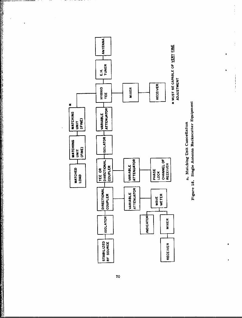
z

zz

w z

44

4 0

w wm co

W m ,

w 4

z -4

'70

w 4

wLza:

m X J

a.

w-

71

4%zZ4

zzp

-x4

w±z

z

uJ

o >

CL- x

0 0n

u4)

ww

z) V) z

27

LI __

a good seal. For this reason the assembly should be first put together with regular

bolted joints until final arrangement of the pieces is settled.

Avoid flexible coaxial line and, insofar as possible, flexible waveguide. At

2 GHz and above all rf lines from the transmitter output should be rigid coaxial

line or waveguide with connecting pieces fabricated to fit. Even short sections

should be adequately supported so that they are vibration free. Flexible coaxial

lines from the mixers to receivers have not been found to cause any problems as

long as they are within loss tolerances specified by the receiver manufacturer.

It is assumed that the assembly for each frequency band will be permanentlyassembled on Its own base and for use slide into equipment racks located in the rf

equipment space (Figure 4). These racks must be very solid with no motion or

vibration and rock steady. For the lowest frequencies at least, the experiments

will be centered vertically in the chamber, so the racks must be perhaps 10 ft tall.

Because of the desirability of operating at lower heights whenever possible, it isrecommended that the racks be of modular construction with top sections removable.

The equipment assemblies on their base could slide into grooves in the racks, held

In place securely by spring tensional rubber rollers. A personnel stand and stairs

with railings to permit comfortable working height and meeting safety requirements

will also be required. It Is recommended that this stand be completely separate

from the equipment rack so that motion by personnel on the stand cannot cause

even the slightest movement of the equipment rack.The transmitting source should be located close to the transmission line assem-

bly and could well be located in the lower portion of the equipment rack, thereby

helping to provide stability for the rack.

As meritioned earlier, if slide-in capability for several transmission linie

assemblies is provided in the rack, it might be possible to leave several assemblies

including their antennas permanently in place. In some cases, at least, antennas

will be mounted separately from the equipment and the possibility of small vertical

movements of the equipment assemblies should be provided for purposes of align-

ment. For assemblies not in current use, slide-in storage racks should be pro-

vided in the rf equipment space. A sketch of one possible general form of the

equipment rack is given in Figure 20.In addition to the components shown in Figures 18 and 19, a bench test setup

will be needed for each frequency band. At a minimum this should consist of aslotted line, probe, SWR meter, waveguide to coaxial adaptors, and at least one

extra matched load. A power meter with thermistor or other appropriate heads for

each band should be available.Also, in addition to the components identified in Figures 18 and 19, a number

of E and H plane 900 bends will be necessary along with several feet of waveguideand separate flanges and chokes so that sections of connecting waveguide can be

S THREADED KNURLED

RINGS

o o o o SLIDE-IN HOLDER FOR

EQUIPMENT BASES0 0 0 0 (SPRING-LOADED ROLLERS)

HOLLOW PIPES

STEEL THREADED SECTION

w EXTENDS APPROX. IFTINTO HOLLOW PIPES

L BOTTOM SECTION TOCONTAIN RF TRANSMITTINGSOURCE

48 ol- HOLLOW STEEL PIPES

Figure 20. Equipment Racks

74

fabricated as necessary to connect the components, and to connect the rf source

to the assembly.

A coaxial assembly will be the most convenient for frequencies from I GHz to

4 GHz and may be usable to 8 GHz. However, use beyond 4 GHz is unlikely.Therefore, waveguide assemblies will probably be needed for 4 to 8 GHz and8 to 12 GHz but use of coaxial components to 8 GHz is worth trying, provided suf-

ficient bandwidth can be found in all of the necessary components.

The following list includes sufficient components for any of the assemblies of

Figures 18 or 19. The components are listed in terms of waveguide but in most

cases direct coaxial line equivalents can be found. In the case of tees and bends,

fewer coaxial ones would be needed because there Is no E or H plane distinction.

Table 7. List of Transmission Line Components

Quantity Item

3 Isolators

4 Directional couplers (I to 10 dB, I to 20 dB, 2 to 40 dB)

2 Variable attenuators (0 to 50 dB or 0 to 100 dB, uncalibrated)

I Variable attenuator, calibrated (0 to 50 dB)

2 Rotary Vane Precision Attenuator (1 - 0 to 100 dB,I - 0 to 10 dB preferred)

2 Rotary vane precision phase shifters

2 E.H. tuners

1 1800 hybrid (very high quality, solid)

2 Matching units, very fine adjustments (3 or 4 preferable forhigher frequencies)

4 Matched loads (3 needed, 1 optional)

5 E-Plane 900 bends

5 H-Plane 900 bends Some number of these will berequired for assembly. If a

E-Plane tees laboratory stock is available,3 H-Plane tees these components can be1 3 ft section waveguide danfo htsok

12 ea flanges and chokes

Optional but Needed for Occasional Use

1 Slotted line with probe (or network analyzer)

2 Waveguide to coaxial adaptors

1 Matched load

I SWR meter

1 Power meter

75

A1

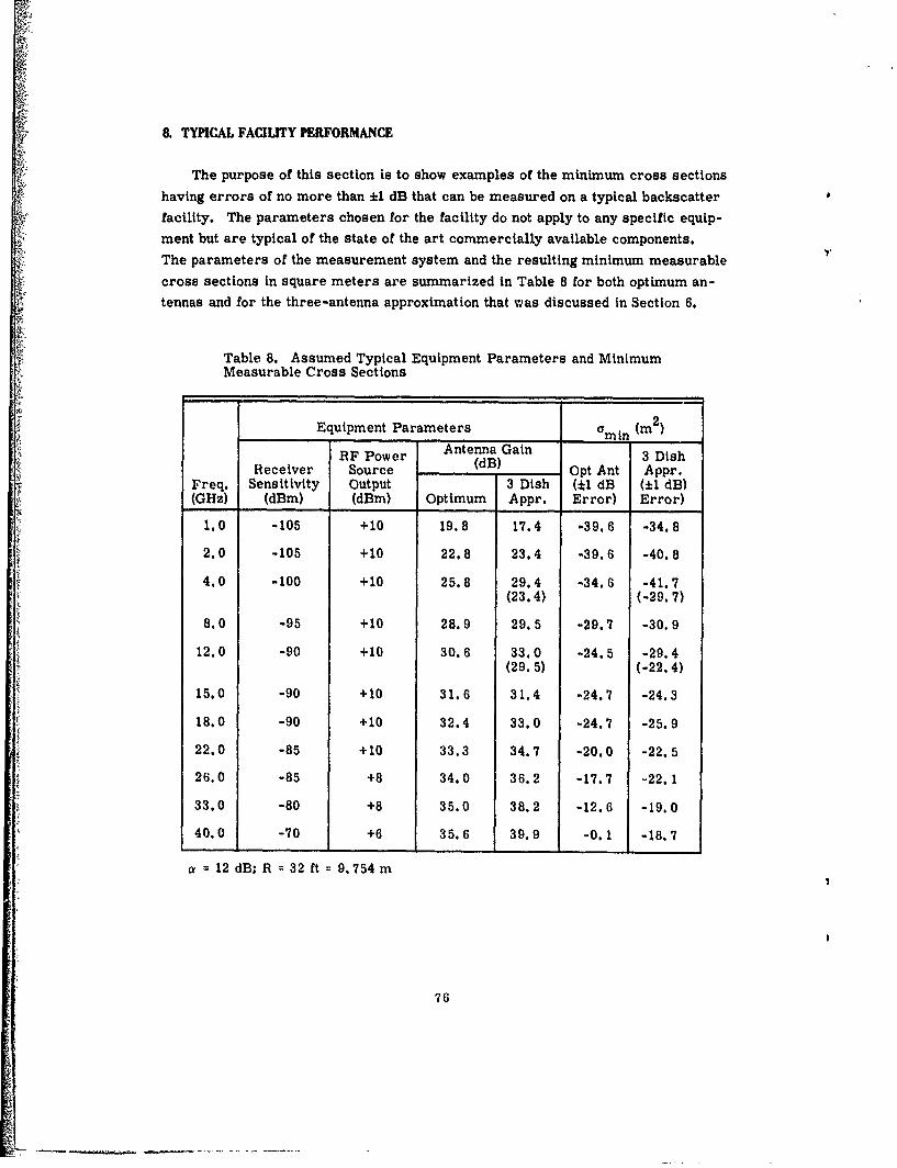
8. TYPICAL FACILITY PERFORMANCE

The purpose of this section is to show examples of the minimum cross sections

having errors of no more than ±1 dB that can be measured on a typical backscatterfacility. The parameters chosen for the facility do not apply to any specific equip-

ment but are typical of the state of the art commercially available components.

The parameters of the measurement system and the resulting minimum measurable

cross sections in square meters are summarized in Table 8 for both optimum an-tennas and for the three-antenna approximation that was discussed in Section 6.

Table 8. Assumed Typical Equipment Parameters and MinimumMeasurable Cross Sections

Equipment Parameters amIn (m2

RF Power Antenna Gain 3 DishReceiver Source (dB) Opt Ant Appr.

Freq. Sensitivity Output 3 Dish (-1 dB (±1 dB)(GHz) (dBm) (dBm) Optimum Appr. Error) Error)

1.0 -105 +10 19.8 17.4 -39.6 -34.8

2.0 -105 +10 22.8 23.4 -39.6 -40.8

4.0 -100 +10 25.8 29.4 -34.6 -41.7(23.4) (-29.7)

8.0 -95 +10 28.9 29.5 -29.7 -30.9

12.0 -90 +10 30.6 33.0 -24.5 -29.4(29.5) (-22.4)

15.0 -90 +10 31.6 31.4 -24.7 -24.3

18.0 -90 +10 32.4 33.0 -24.7 -25.9

22.0 -85 +10 33.3 34.7 -20.0 -22.5

26.0 -85 +8 34.0 36.2 -17.7 -22.1

33.0 -80 +8 35.0 38.2 -12.6 -19.0

40.0 -70 +6 35.6 39.9 -0.1 -18.7

a 12 dB; R 32 ft = 9.754 m

76

Assumptions underlying the calculations are:

1. The measurement system is a backscatter facility with a single transmit/

receive antenna.

2. The maximum useful range for measurements is R = 32 ft (9.754 m) and

all measurements are made at this range.

3. The antennas are 60 percent efficient with gains given by Eqs. (50) and (53).

4. There is a total loss of 12 dB in the transmission line components. This

is composed of a 6 dB loss in the hybrid tee, a 5 dB loss in the detecting or mixing

crystal, and 1 dB of miscellaneous losses.

5. The minimum detectable signal of the receiver and the output of the signal

generator vary over the frequency band of I GHz to 40 GHz approximately as shown

in Table 8.

6. Miscellaneous background reflections and the uniformity of the incident

field over the model space are not the factors limiting measurement accuracy.

7. The minimum measurable reflected signal must be 20 dB greater than the

minimum detectable signal of the receiver, resulting in a ±1 dB uncertainty in the

measured results.

The resulting minimum measurable cross sections, amin' in square meters

are shown in Figure 21 as a function of frequency for both optimum antennas and

for the three-antenna approximation. As can be seen from Table 8, the decrease

in minimum measurable cross sections at the higher frequencies is due to the

assumed decrease in the receiver sensitivity and output of the signal source at the

higher frequencies. The use of stable amplifiers to boost the output of the signal

source would improve amin at these frequencies in a direct relation to the gain of

the amplifier.

The scale factor from 1 GHz to 40 GHz is 40, or 1600 in area, and equivalent

to 32 dB. Hence, with the 12 in. dish, cross sections of about 13.3 dBSM or

2.14 m 2 at L-Band could be scaled to 40 GHz and measured with a ±1 dB error.

Similarly, with the 18 in. dish, L-Band cross sections of about 0. 1 m2 could be

measured at 10 GHz, while L-Band cross sections as low as -35 dBSM could be

measured at L-Band directly.

In Figure 22 the maximum antenna size, the maximum model size, and the

working distance between half power points of the beam at the model space are

shown as a function of frequency for measurement ranges from R = 32 ft to

R = 72 ft. These curves are based on the conventional far field criterion. If half

of this distance is to be used for measurements, R = D2 /k instead of R = 2D 2 /X, the

resulting antenna size is multiplied by a factor of approximately 1. 4. This value

can be obtained from Figure 22 by choosing the antenna size corresponding to a

value of R that is twice as large at the desired frequency.

77

0

5.0I

-10 IOPTIMUM 4

-15 ANTENNAS ,/

-20 -22

25 -ISIN. / P 2IN.b DISH DS

.30 -

361N1-40 - -- DISHI

-45-

-501o 1 I I I I I a h 1 1 !II

0 Q q000 q 0 0O0 0 i 010

FCGHZ)

Figure 21. Minimum Measurable Cross Sections with*1l dB Error with Typical Backscatter Facility (forfacility parameters see Section 8)

6.0., ,* 12.0

R(F'T)

5.0 64 10.056 uss/X

484.0- 40 81.0

~3.0 - 2 6.0E

2o 4.OQO 00

1- 2.01 S

F(WO~

Figure 22. Maximum Model Size, Maximum AntennaSize, and Half Power Beam Distances for f 1 GHzto 40 GHz at Various Measurement Distances

78

References

1. Blacksmith, P., Hiatt. R. E., and Mack, R. B. (1965) Introduction to radarcross section measurements, Proc. IEEE 53:901-920.

2. Silver, S. (1949) Microwave Antenna Theory and Design, Vol. 12, RadiationLaboratory Series, McGraw-Hill Book Company, Chap. 6.

3. Kerr, D. E. (1951) Propagation of Short Radio Waves, Vol. 13, RadiationLaboratory Series, McGraw-11ill Book Company, Chapts. 4 and 6.

4. Skolnik, M. I. (1968) Introduction to Radar Systems, McGraw-Hill BookCompany, Chapts. 1 and 7.

5. Van De Hulst, 11. C. (1957) Light Scattering by Small Particles, John Wiley& Sons, Inc., New York, Chapt. 9.

6. Freeny, C.C. (1966) Target support parameters associated with radar reflec-tivity measurements, Proc. IEEE 53:929-93 6.

7. Knott, E. F. and Senior, T. B. A. (1964) Studies of Scattering by Cellular PlasticMaterials, Report No. 5849 -1 -F. The Radiation L.aboratory, Univ. of Mich.,Ann Arbor, Mich.

8. Senior, T.B.A., Plonus, M.A., and Knott, E.F. (1964) Designing foamedplastic target supports, Microwaves, 38-43.

9. Mack, R.B., Wojcicki, A.W., and Andriotakis, J.J. (1973) An Imelementationof Conventional Methods of Measuring the Amplitude and Phase of Backscatotered Fields, AFCRL-TR-73-0418, AD 770 015.

IA

79J