Embed Size (px)
Citation preview

In: Outsourcing, Team Work and Business Management ISBN: 978-1-60692-073-2Editors: J.E. Moran et al, pp. 1-31 © 2008 Nova Science Publishers, Inc.
Chapter 1
THE IMPORTANCE OF CONTEXT IN DETERMININGCONSUMER RESPONSE TO FOOD SAFETY EVENTS:THE CASE OF MAD COW DISEASE DISCOVERY IN
CANADA, JAPAN AND THE UNITED STATES1
Sayed Saghaian, Leigh Maynard and Michael ReedUniversity of Kentucky
Abstract
Introduction
No food safety threat inspires more dread than variant Creutzfeldt - Jakob disease(vCJD), an irreversible brain wasting disease contracted from eating beef infected withBovine Spongiform Encephalopathy (BSE). Consumers often refer to vCJD and BSEinterchangeably as “mad cow disease,” which can induce fear through uncertainidentification, long incubation periods, and devastating symptoms. Even though most
1 This chapter is Journal Paper Number 08-04-028 of the Kentucky Agricultural Experiment Station.
Sayed Saghaian, Leigh Maynard and Michael Reed2
countries have experienced very few BSE cases, such as Japan, the United States, andCanada, and the risk may be exceedingly low, previous studies found conflicting consumerresponses to BSE in these low-incidence countries. This chapter helps reconcile disparities inprevious findings by demonstrating the importance of context in determining consumerreactions to a BSE scare. The results help focus attention on strategic risk managementoptions that agribusiness managers can use to guard against shocks to retail beef demand ifand when future BSE events occur.
This chapter consists of three parts that present two complementary statistical analyses.In the first part, we show consumer reactions to BSE in Japan using Directed Acyclic Graphsand historical price and quantity decompositions. The Japanese beef markets faced twosubsequent cases of BSE discoveries in 2001, eroding consumer confidence in beef supplychannels with huge economic losses to the Japanese beef industry. In the second part, we lookat BSE’s impact along the U.S. supply chain using similar contemporary time-series methods.The U.S. beef industry faced BSE in 2003, which led to differential impacts on farm,wholesale, and retail markets. Relative to the U.S., Japanese consumers have a strongpreference for domestically produced beef, encouraged by retail country-of-origin labelingand BSE media coverage critical of imported beef. Consistent with these differences inpreferences, marketing, and information, we observe more negative and more nuancedreactions to BSE in Japan versus the U.S.
The third part highlights contextual differences in Canada. A double-hurdle model ofCanadian fast food beef purchases shows no significant BSE impacts on the likelihood orquantity of fast food beef item purchases. When applied to Canadian supermarket beefpurchases, however, a striking pattern emerges. After the initial BSE event in 2003, whenmedia coverage focused mainly on the plight of ranchers, beef demand increasedsignificantly. Moreover, demand increased the most in Alberta, the center of Canada’s beefindustry. Following two later BSE events, beef demand fell significantly. The results illustratethe importance of context along at least five dimensions: the food purchase venue, thegeographic proximity of consumers to BSE events, the ordering of BSE events, the role ofsupplier behavior, and the nature of media coverage.
Part I: BSE Discoveries in Japan
The first case of BSE in Japan was reported in September 2001. BSE is a fatalneurological disease which typically occurs in adult animals. BSE is primary transmitted byfeeding of diseased animal products. Consumption of contaminated beef by humans issuspected to cause vCJD. BSE discovery in Japan caused considerable economic damage tothe Japanese beef and food service industries, in part due to the actions of Japanese officialsthat eroded consumer confidence (McCluskey, et al. 2004). The Japanese government’sresponse to the crisis was an aggressive marketing campaign promoting the safety of Japanesebeef, which had salient impacts on Japanese consumer reactions (Fox and Peterson, 2002).
The impact of food safety scares has been extensively investigated in the literature. Thesestudies generally show that food safety scares affect prices and demand adversely, and thatconsumers are willing to pay higher premiums for safety and quality assurance (e.g., Marsh,Schroeder and Mintert, 2004; Piggott and Marsh, 2004; McCluskey, et al., 2004; Peterson andChen, 2005; Livanis and Moss, 2005; and Chopra and Bessler, 2005). Increased awareness of

The Importance of Context in Determining Consumer Response… 3
food safety problems appears to create opportunities for branding, labeling, and productdifferentiation through traceability and beef quality. Labeling of credence attributes for beefreduces information costs to consumers and can result in increased demand for quality-assured products. Beef producers and retailers can differentiate their beef products to earnhigher premiums, by using beef safety and quality as a strategic response to consumers’ beefsafety concerns.
We investigated the impact of BSE events on Japanese retail meat demand with beefdifferentiated by quality and country of origin. We used a cointegrated vector error correction(VEC) model, directed acyclic graphs, and historical decomposition to find Japaneseconsumer responses to the sudden, unexpected beef safety scares. Directed graphs allow theerrors among the endogenous variables to be incorporated into the forecasted effects of thesemeat market shocks over time. We traced the dynamic effects of these shocks on retail-levelmeat prices and quantities over time to see if these changes were consistent with well-informed consumer behavior.
The Data
Fish, poultry, and four beef types differentiated by type and country of origin, namely,U.S., Australian, Japanese wagyu, and Japanese dairy beef, were evaluated. The sample datafor fish and poultry were not distinguished by source of origin. The sample contained 105observations from April 1994 to December 2002. Retail beef prices and quantities wereobtained from Agriculture and Livestock Industries Corporations (ALIC) data. Beef priceswere the weighted prices of four cuts (chuck, loin, round and flank) reported by ALIC basedon Nikkei Point-of-Sales data. Retail prices and quantities for fish and poultry were obtainedfrom the Retail Price Survey by the Statistical Bureau Ministry of Public Management, HomeAffairs, Post and Telecommunications. Fish prices were the weighted average of tuna, horsemackerel, flounder, yellow tail and cuttlefish. The fish types selected are composed of high,medium and low-end fish types and reflect the most representative fish series for which datawere available and complete.
The Empirical Model
Empirical models applied to food safety events cover a wide range, from the commonlyused Almost Ideal Demand System, the Rotterdam demand system, and related variations, tomodels of contingent valuation, experimental auctions and conjoint analysis. Themethodological approach used in this study includes a VEC model, directed acyclic graphs,and historical decomposition to investigate the dynamics of price and quantity changes. TheVEC model not only allows estimates of short-run relationships for the price and quantityseries, but it also preserves the long-run relationships among the variables. Historicaldecompositions aid in providing a visual explanation of the shock’s impact on price andquantity series in the neighborhood of each incident. Orthogonal innovations are constructedusing graph theory to determine causal patterns behind the correlation in contemporaneousinnovations of the VEC model.

Sayed Saghaian, Leigh Maynard and Michael Reed4
The first step is stationarity testing of each series using the Augmented Dickey-Fuller(ADF) test. The test involves running a regression of the first difference of the series against theseries lagged one period, lagged difference terms, and a constant. The stationarity test checksthe series for unit roots. The non-stationary series are integrated of order one or I(1) with thefirst differences being stationary or I(0). Johansen’s co-integration test is performed todetermine whether the series are co-integrated. Having a co-integrating equation captures thelong-run relationship among the variables. In this process, a matrix is found to capture the long-run relationship among the variables. That matrix is decomposed into two matrices, α and β,where the matrix β contains the co-integrating vectors representing the underlying long-runrelationship, and the α matrix describes the speed of adjustment at which each variable movesback to its long-run equilibrium (Johansen and Juselius, 1992; Schmidt, 2000).
The VEC model’s covariance matrix helps when investigating the causal relationshipamong the variables with directed acyclic graphs (Bessler and Akleman, 1998; Saghaian,Hasan, and Reed, 2002). With this method, an algorithm determines the causal structurebehind the correlation in the errors of the variables (Swanson and Granger, 1997). Finally,historical decompositions break down the price/quantity series into historical shocks in eachseries to determine their responses in a time interval neighborhood of the BSE events.
The Results
Table 1 presents the OLS estimation results of the unit-root tests. The second column ofthe table shows the tests failed to reject the null hypothesis of zero first-order autocorrelationat the 5% level of significance except for fish price, poultry price, US quantity, and dairyquantity. The right-most column of Table 1 gives the results of the ADF test for the firstdifference transformation of the series. The null hypothesis is rejected for all variables afterfirst differencing.
Table 1. Augmented Dickey-Fuller (ADF)a Test Results.
Variable Test Results for Variablesin Levels
Test Results for Variablesafter First-Differencing
US Beef Price 2.64 9.47**AUS Beef Price 2.39 11.60**Wagyu Beef Price 2.13 11.11**Dairy Beef Price 1.64 13.05**Fish Price 3.02* 7.45**Poultry Price 4.01** 9.40**US Beef Quantity 3.40* 10.09**AUS Beef Quantity 0.90 12.37**Wagyu Beef Quantity 1.40 11.48**Dairy Beef Quantity 2.76* 12.86**Fish Quantity 2.30 4.44**Poultry Quantity 1.98 4.14**
Note: ** 1% significance level, * 5% significance level.a Test statistics are in absolute value and compared to MacKinnon (1996) one-sided p-value.Source: Saghaian and Reed (2007).

The Importance of Context in Determining Consumer Response… 5
Table 2 presents the results of co-integration tests for the price and quantity series. Thenull hypothesis that 0=r , 1≤r , and 2≤r was rejected at the 5% level for the price series,but the null hypothesis of 3≤r could not be rejected at the 5% level. For quantity, the nullhypothesis that 0=r and 1≤r was rejected at the 5% level, but the null of 2≤r could notbe rejected. Thus there are long-term relationships among the variables and the VEC model isappropriate in order to determine the directed graphs and causal patterns for prices andquantities.
Table 2.
Johansen Cointegration Test Results for Prices
Null Hypothesisa Trace Statistics 5% CriticalValue Eigenvalue
0=r * 185.46 95.75 0.531≤r * 109.64 69.82 0.412≤r * 56.34 47.86 0.263≤r 25.44 29.80 0.15
Johansen Cointegration Test Results for Quantities
Null Hypothesisa Trace Statistics 5% CriticalValue Eigenvalue
0=r * 170.37 95.75 0.611≤r * 75.10 69.82 0.272≤r 43.86 47.86 0.19
a r is the cointegrating rank, MacKinnon-Haug-Michelis (1999) p-value. * 5% significance level.Source: Saghaian and Reed (2007).
The residual correlation matrix of the VEC models provided the contemporaneousinnovations (errors) that show how errors among the endogenous variables are related. Theresults show that the strongest correlation exists between the Japanese wagyu and dairy prices(0.68). This makes sense as pricing policies for Japan’s beef industry are consistently appliedto wagyu and dairy beef. The results show the residuals associated with the two importorigins are slightly correlated with dairy, but U.S. residuals are more strongly correlated toresiduals from Japanese wagyu than Australian beef. Finally, there is little correlation inresiduals for U.S. and Australian beef prices or among fish, chicken, and beef prices.However, there is much more correlation among the residuals from the quantity model.Correlations between US and wagyu, US and dairy, and wagyu and dairy are all high amongthe beef quantities. Fish and poultry consumption residuals are also highly correlated. Mostcorrelation coefficients among the quantity errors are 0.40 or above, much higher than forprices.
A formal test of contemporaneous causal structures is performed by orthogonalizinginnovations to obtain the historical decomposition functions. The TETRAD IV software isapplied to the correlation matrix to generate the causal patterns among the price and quantityseries on innovations from the endogenous variables in each system (Spirtes et al., 1999). Thehistorical decompositions include a 12-month horizon for each endogenous variable.

Sayed Saghaian, Leigh Maynard and Michael Reed6
The BSE Impact in Japan
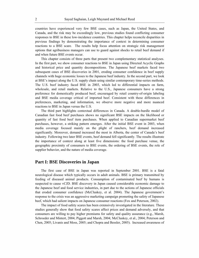
Imported beef prices in Japan fell immediately in response to the BSE discovery, butdomestic beef prices actually increased. However, ultimately all beef prices were adverselyimpacted by the BSE discovery. U.S. beef import prices fell the most dramaticallyimmediately after the BSE discovery and saw the widest difference between the actual andforecasted prices. U.S. beef prices rebounded after the first two months, but they took anotherquick dive after December, reaching their lowest point in May, approximately seven monthsafter the outbreak (Figure 1).
USA Beef Price (BSE01)
July 2001 - June 2002
(Yen
/gra
m)
Jul Aug Sep Oct Nov Dec Jan Feb Mar Apr May Jun2001 2002
0.800
0.816
0.832
0.848
0.864
0.880
0.896
0.912
0.928
Aus Beef Price (BSE01)
July 2001 - June 2002
(Yen
/Gra
m)
Jul Aug Sep Oct Nov Dec Jan Feb Mar Apr May Jun2001 2002
0.50
0.55
0.60
0.65
0.70
JW Price (BSE01)
July 2001 - June 2002
(Yen
/Gra
m)
Jul Aug Sep Oct Nov Dec Jan Feb Mar Apr May Jun2001 2002
1.60
1.62
1.64
1.66
1.68
1.70
1.72
1.74
JD Price (BSE01)
July 2001 - June 2002
(Yen
/Gra
m)
Jul Aug Sep Oct Nov Dec Jan Feb Mar Apr May Jun2001 2002
1.14
1.16
1.18
1.20
1.22
1.24
1.26
1.28
Actual Price: ______________Forecasted price before the event: ----------------------Vertical line is the Event of interest: |Source: Saghaian, Maynard, and Reed (2007)
Figure 1. Impact of BSE 2001 on Beef Prices in Japan.
Australian beef prices had a similar pattern to U.S. prices, but during the first month therewas no dramatic drop. Japanese wagyu and dairy beef prices rose after the BSE outbreak;
The Importance of Context in Determining Consumer Response… 7
certainly not what one would expect, but by December, those prices began to fall absolutelyrelative to what they would have been without an outbreak. The pattern for these beef pricesis explained by the way Japanese authorities handled the news of the BSE discovery. Theimmediate negative responses observed for U.S beef prices is attributed to the publishedremarks of a Japanese meat company who blamed imported beef as the most likely source ofBSE in Japan, as explained by McCluskey, et al. (2004). Two weeks after publiclyannouncing the first confirmed case, a second case contradicted the government’s assurancesof healthy domestic animals, prompting anxiety among consumers and leading to furtherdecline in all beef prices.
The reliability of suppliers and perceived differences among suppliers may explain theimpact of a food safety incident on consumers and their loss of confidence or trust (Bockerand Hanf, 2000). When it comes to food safety and reliability, consumers differentiate amongproduct brands and origins, and trust in suppliers and retailers plays a major role in theirpurchasing decisions. Because consumers are unaware of unsafe food, a priori, and rely onsupplier credibility and reputation; any news of a food safety scare involving a particularsupplier impacts their perceptions and judgments regarding the reliability of that supplier.Becker et al (1996) showed that ‘trust/safety’ was one of the main factors influencing Germanconsumer choice of a particular meat-product retailer. In an experimental study, Bocker(2002) tested the hypothesis that consumer reaction to a food safety scare could be explainedby differences among perceived reliability of suppliers.
The results indicate Japanese consumers reacted to the differentiation between suppliersin terms of their riskiness, increasing their confidence in the domestically produced beef;Japanese consumers’ beef purchase decision was impacted by the perception of reliability ofbeef suppliers. Customers did not abandon all beef, but differentiated beef by perceivedriskiness of the source. Bocker and Hanf (2000) showed that with BSE in Germany,consumers switched to local butcheries that they trusted more for safer products. With thesecond announcement of a BSE discovery and the perceived discrepancy in the news andamong suppliers, all beef prices were adversely impacted, indicating erosion of consumertrust and confidence in the entire beef industry.
Our results show that the negative effects of the first BSE shock on beef prices dissipatedafter a few months, but the second wave of the scare had a stronger impact on beef prices.Mazzocchi (2005) found similar results regarding two instances of BSE crises in Italy. Ourresults show that while there was concern about all beef in Japan, Japanese domestic beefprices fell less than imported prices, which suggests that despite the BSE outbreaks, Japaneseconsumers still had more confidence in domestic beef production. Yet after twelve months,consumption of all types of beef was markedly lower than the predictions without a BSEincident.
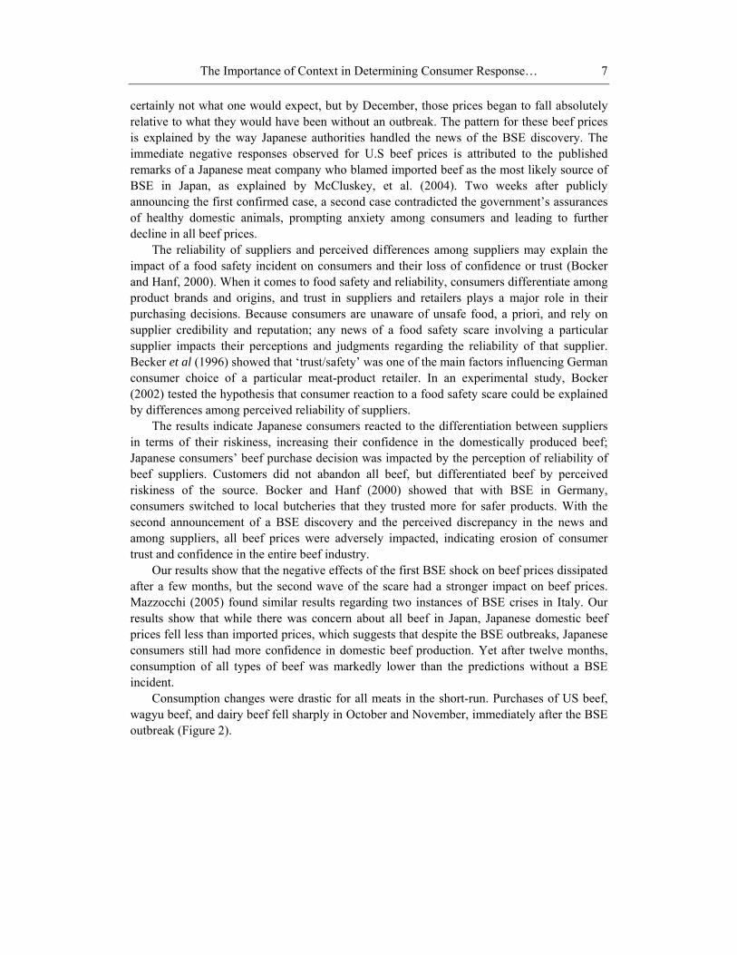
Consumption changes were drastic for all meats in the short-run. Purchases of US beef,wagyu beef, and dairy beef fell sharply in October and November, immediately after the BSEoutbreak (Figure 2).

Sayed Saghaian, Leigh Maynard and Michael Reed8
BSE impact on cosumption of US
Log
Per
Cap
ita
Apr May Jun Jul Aug Sep Oct Nov Dec Jan Feb Mar Apr May Jun2001 2002
1.8
2.1
2.4
2.7
3.0
3.3
3.6
3.9
4.2
BSE impact on cosumption of WAGYU
Log
Per
Cap
ita
Apr May Jun Jul Aug Sep Oct Nov Dec Jan Feb Mar Apr May Jun2001 2002
2.00
2.25
2.50
2.75
3.00
3.25
3.50
3.75
BSE impact on cosumption of DAIRY
Log
Per
Cap
ita
Apr May Jun Jul Aug Sep Oct Nov Dec Jan Feb Mar Apr May Jun2001 2002
3.25
3.50
3.75
4.00
4.25
4.50
4.75
Source: Saghaian and Reed (2007).
Figure 2. The BSE impact on per capita consumption of U.S., wagyu, and dairy beef in log-form.
In contrast, consumption of grass fed Australian beef, fish, and poultry increased sharplyduring the same period (Figure 3).

The Importance of Context in Determining Consumer Response… 9
BSE impact on cosumption of AUS
Log
Per
Cap
ita
Apr May Jun Jul Aug Sep Oct Nov Dec Jan Feb Mar Apr May Jun2001 2002
3.85
3.92
3.99
4.06
4.13
4.20
4.27
4.34
4.41
BSE impact on cosumption of FISH
Log
Per
Cap
ita
Apr May Jun Jul Aug Sep Oct Nov Dec Jan Feb Mar Apr May Jun2001 2002
5.65
5.70
5.75
5.80
5.85
5.90
5.95
6.00
BSE impact on cosumption of POULTRY
Log
Per
Cap
ita
Apr May Jun Jul Aug Sep Oct Nov Dec Jan Feb Mar Apr May Jun2001 2002
5.4
5.5
5.6
5.7
5.8
5.9
6.0
6.1
Source: Saghaian and Reed (2007).
Figure 3. The BSE impact on per capita consumption of fish, poultry, and Australian beef in log-form.
The impact clearly indicates that consumers were mostly suspicious of US beef comparedto other beef and had much greater trust in fish and poultry, where consumption drasticallyincreased. This shows consumers switched to meats considered to be free of a BSE threat.

Sayed Saghaian, Leigh Maynard and Michael Reed10
These results indicate that Japanese consumer’s purchasing decisions were consistent with theinformation they were given. While in the short-run consumption of beef decreased, in thelonger run, all meat consumption levels were close to the predictions without a BSE incident;but prices, and consequently profit margins, were lower. These results showed that Japaneseconsumers first reacted negatively to the beef safety scares and changed their buying andconsumption habits accordingly, and over time, as the concerns dissipated and beef safetyworries diminished, they reverted back to their previous consumption pattern. These resultsare consistent with discussions made by Mazzocchi (2005).
These insights into the habits of consumers and the changing purchasing patterns formeat consumers faced with food safety concerns have strategic implications for supply chainmanagers and practitioners. It is very important for food firms to be active in providinginformation to consumers because such information is used in purchasing decisions. Yet theinformation conveyed must be reliable if trust is to be retained between producers andconsumers. Baker (1998) shows consumers are demanding more food safety information; helists several private, as well as government policy, options (such as labeling, increasedproduction standards and regulatory monitoring) that can help address those concerns.
Remarks
The effects of food safety scares are part of a dynamic process, where consumers changeconsumption during the scare and often return to their past behavior afterward. This studyfinds that consumers over-react initially to the shock with decreased consumption of thesuspect food item, but concern gradually dissipates, leading to the establishment of a newequilibrium. Japanese consumers understood the differences in the two beef safety scares andreacted differently to them. Prices of all beef products were lower twelve months after theBSE discovery, a clear indication that the news of the BSE discovery adversely affectedconsumers’ perceptions of beef quality and lowered profit margins. Yet, the price decrease forthe two imported beef types were more than the price decrease for the two domesticallyproduced beef categories. This indicates that Japanese consumers have a more positive viewof their own beef products and this keeps the price of their domestic beef products fromfalling as much as imported products. Japanese consumers moved away from beef that useshigh levels of concentrated feeds (US beef, wagyu beef, and dairy beef) and flocked towardgrass fed Australian beef and fish and poultry.
These results provide incentives for beef producers and retailers to proactively informconsumers about ongoing beef safety measures, and can potentially provide policy makers abasis for countermeasures and compensations. Beef safety crises have increased the need forrobust information technologies in the food marketing system. Time and experience provide ametric for consumers to recalibrate their risk perception and require beef producers andmarketers to pay greater attention to beef safety issues and employ quality assurancemeasures and traceability schemes to address consumer concerns. The BSE situation hascertainly created opportunities for producers that have traceable production systems and havequality assurance programs that involve branding and labeling.
Proactive information provision in the food marketing systems reduces the impacts of thefood scare. Safe food seems to be largely a public good, so industries have an interest todevelop protocols together to provide greater safety assurances. A BSE case or salmonella

The Importance of Context in Determining Consumer Response… 11
outbreak impacts everyone; one incidence of ‘bad strawberries’ hurts the whole strawberryindustry and even related fruits. The U.S. government and the food industry must continue toinvest heavily into procedures that will reduce food safety scares in these areas and intoinformation systems that minimize the impacts of food safety shocks.
Part II: BSE Discovery in the U.S.
While discovering BSE in other countries such as the United Kingdom and Japan resultedin considerable economic damage to beef producers as well as food service industries, thenotable impact of the BSE discovery in the U.S was mostly on the export sector; Japan, amajor export market for U.S. beef and beef products stopped all imports. Quickly after theU.S. BSE discovery in December 2003, USDA announced additional beef safety proceduresthat banned specified risk material (SRM), such as brain, spinal tissue, etc., for cattle over 30months of age from food supply.
This part focuses on the short-run dynamics of price adjustment and transmission to seehow the beef safety scare affected the price margins along the U.S. beef supply channel.Research on vertical and spatial price transmission is vast, expanding in different directionsfrom asymmetric price transmission, price stickiness and incomplete pass through, to marketefficiency and integration, to concentration and market power. Given recent structuralchanges in the U.S. beef industry and its high market concentration, an important researchquestion is the extent that the BSE shock was transmitted through the supply chain andimpacted prices at the feedlot, packer, and retail levels. Factors such as product heterogeneity,long-term contracts, and market concentration can potentially influence the degree anddynamics of price transmission, leading to differential price effects along the marketing chain.Differing transmissions for the shock have welfare implications with respect to the efficiencyand equity of the marketing system.
There are many research articles on market integration and price transmission along theagricultural marketing channels. Early models were primarily static linear equilibriummodels, assuming perfectly competitive markets. An important example of this literature isthe work of Gardner (1975). Market integration and price transmission theory has evolvedextensively since Gardner’s seminal work, expanding the literature in different directions.Heien (1980) added dynamic analysis to address short-run disequilibrium price adjustments.Tiffin and Dawson (2000) found that UK lamb prices were determined in the retail market,and then passed upward along the supply chain. Goodwin and Holt (1999) and Goodwin andHarper (2000) found that retail market shocks were confined to retail markets, but farmmarkets adjusted to shocks in wholesale markets. Yet, Ben-Kaabia, et al. (2002) found bothsupply and demand shocks were fully passed through the marketing channel; i.e., they foundcomplete price transmission.
The literature on price stickiness and incomplete price transmission provides a detailedexplanation for asymmetric price behavior. Price transmission can be asymmetric when thereexits different speeds of price adjustment across vertically linked markets. Price asymmetrycan exist with respect to magnitude, speed, or a combination of the two. It is important to notethat there are different definitions of price asymmetry. In this research the focus is on thedifferent speeds of price adjustment along the beef marketing channel in the feedlot,wholesale and retail markets affecting price margins. The traditional definition of price

Sayed Saghaian, Leigh Maynard and Michael Reed12
asymmetry refers to a situation where producer price increases are passed forward quickerand more completely to consumers than price reductions (Pelzman, 2000; Bakucs and Ferto,2005).
In an efficient market prices are transmitted fully and completely. The fact that pricedynamics may differ under competitive and noncompetitive market conditions can lead tomarket inefficiency. McCorrison et al. (1998) demonstrated the role of oligopoly power indetermining the price transmission elasticity following a supply shock. Other studies havesupported the hypothesis that market concentration and imperfect competition can be thecause of asymmetric price transmission (Miller and Hayenga, 2001; Lloyd, et al., 2003).Luoma, et al. (2004) has argued that market power is the most likely explanation forasymmetric price transmission in the long run. Retailers may keep price levels relatively fixedfor long periods when markets are imperfectly competitive, or oligopolies may react quickerto declining margins by utilizing their market power. They do this to maintain market shares,keeping long-run rather than short-run profits in mind. Hence, market power can reduce pricetransmission along the marketing chain.
The Data, the Model, and the Empirical Results
Weekly data for feedlot, wholesale, and retail prices were assembled from the LivestockMarketing Information Center (LMIC) for 1/5/1991 to 7/2/2005. The vertical structure of thedata set begins with feeder cattle followed by live cattle, wholesale, and retail levels. Allprices are in dollar per hundred weights ($/cwt). The feedlot price used in this analysis is theKansas live cattle price. A 1000 lb steer is assumed, and multiplied by this Kansas price, toderive a live steer value. The total wholesale value is the sum of the boxed beef value and thebyproduct value -- both are USDA prices from the LMIC. From this assumed 1000 lb steer, adressing percentage of 63% and a retail yield of 42.7% from the live animal weight are usedto calculate the retail value, which is the monthly USDA reported retail price multiplied bythe estimated retail yield. The beef prices are the average for all grades.
The assumption is that the BSE discovery reported by the news outlets affects qualityperception of all beef, consistent with other research in this area (e.g., Piggott and Marsh,2004). While the beginning date of the BSE scare is well known, there is no way to knowexactly how long the beef safety scare will impact on consumer perceptions of safety. In thisresearch we concentrate on the short-run dynamics of price adjustment and price transmissionat different market levels in a neighborhood around the BSE shock specified by the historicaldecomposition graphs, though price transmission patterns could be different before and afterthe BSE scare.
In this part, we closely followed the contemporary non-stationary time-series modelingparadigm of the previous section. First, the temporal properties of the three price series wereanalyzed using ADF tests. We failed to reject the null hypothesis of a unit root for thesevariables with two terms, a constant and a trend. Each series was then first differenced and theADF regressions were re-estimated with a constant but no trend. In each case, we rejected thenull hypothesis of a unit root at the 1% level of significance.
Second, Johansen’s cointegration tests were employed to determine if a long-runrelationship existed among the three variables in the system. These results suggested there aretwo long-run equilibrium relationships between the three price series (Table 3).

The Importance of Context in Determining Consumer Response… 13
Table 3. Johansen Cointegration Test Results
Null Hypothesisa TraceStatistics
5% CriticalValue Eigenvalue
0=r * 80.56 29.80 0.081≤r * 17.63 15.49 0.022≤r 2.03E-05 3.81 0.051
a r is the cointegrating rank.*Denotes rejection of the hypothesis at the 5% level.Source: Saghaian (2007).
Next, we estimated a VEC model and conducted hypothesis testing within thisframework. The VEC model analysis of dynamic adjustments provided a precise measure ofprice transmission speeds. The empirical estimates of the adjustment speeds are summarizedin the top portion of Table 4. The adjustment speeds for wholesale and retail prices werestatistically significant at the 1% level. The adjustment speed for feedlot prices was notstatistically significant. The dynamic adjustment speed for wholesale prices was much higher,0.13, (in absolute value) than retail prices, 0.02. This is an interesting result suggesting thatwith the beef safety shock, wholesale prices must adjust much more and do it faster than retailprices to restore the long run equilibrium. These results indicate that the speeds of priceadjustment vary by market and prices in the wholesale market adjust more than six timesfaster to the BSE shock than prices in the retail market.
Table 4. The Empirical Estimates of Speeds of Adjustment and Diagnostics
Variable ftPΔ wtPΔ rtPΔSpeeds of Adjustment -0.01 -0.13* -0.02*Model Diagnostics 2R 0.14 0.39 0.13 AIC -4.79 -5.38 -7.17 Schwarz Criterion -4.70 -5.29 -7.08
* 1% significance level.Source: Saghaian (2007).
Some explanations given in the literature for the causes of price asymmetry are productheterogeneity, long term contracts, and adjustment or menu costs (e.g., Goodwin and Holt,1999; Zachariasse and Bunte, 2003), which may explain the differential speeds of priceadjustment along the U.S. beef marketing channel. Originally, Hicks (1974) and Okun’s(1975) works showed that prices in some sectors of the economy were sticky while prices inother sectors were flexible. According to their arguments, prices of most goods and servicesare not free to respond to changes in demand in the short run. Bordo (1980) showed someprices respond slowly to policy shocks due to long-term contracts.
We employed Granger causality tests and directed acyclic graphs to investigate the causalpatterns among the variables. The covariance matrix of the VEC model was used toinvestigate the causal relationship among the variables by directed acyclic graphs. The resultsshow that innovations in feedlot and wholesale, and in wholesale and retail price variables
Sayed Saghaian, Leigh Maynard and Michael Reed14
affect residuals in each other, but there are no arrows to indicate direct causality. Also, thereexists no residual relationship between feedlot and retail beef prices. The relationshipbetween feedlot and retail beef price residuals is through wholesale prices.
Since directed graph results from the residuals did not provide a clear causality direction,we used pairwise Granger causality tests (with four lags) to investigate causal directions. Theresults are summarized in Table 5. F-test results indicate that the hypothesis, retail prices donot Granger-cause feedlot prices, is the only one that cannot be rejected. The results show thedirection of causality runs especially strong from feedlot to wholesale to retail prices.However, this relationship is not unique (i.e., uni-directional); there are causality relationshipsgoing upstream, from retail to wholesale to feedlot prices, as well.
Table 5. The Results of Pairwise Granger Causality Tests
Null Hypothesis F-Statistic
Feedlot Price does not Granger Cause Wholesale Price 41.94**Wholesale Price does not Granger Cause Feedlot Price 7.01**Wholesale Price does not Granger Cause Retail Price 17.07**Retail Price does not Granger Cause Wholesale Price 4.88*Feedlot Price does not Granger Cause Retail Price 12.49**Retail Price does not Granger Cause Feedlot Price 1.73
** 1% significance level, * 5% significance level.Source: Saghaian (2007)
The results rejected the hypothesis that price transmission in the U.S. beef sector flowsonly downward along the supply chain with the direction of causality running from producerto retail prices. These results suggest that prices in the U.S. beef sector are not determined atone end and then passed down or up along the supply channel; pricing patterns in the U.S.beef sector are not just cost or demand driven. Prices are determined simultaneously throughbidirectional interaction between the different stages (likely through contracts).
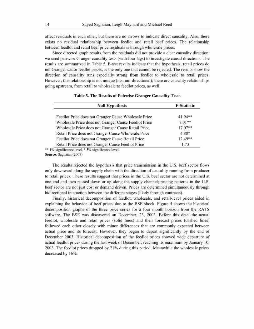
Finally, historical decomposition of feedlot, wholesale, and retail-level prices aided inexplaining the behavior of beef prices due to the BSE shock. Figure 4 shows the historicaldecomposition graphs of the three price series for a four month horizon from the RATSsoftware. The BSE was discovered on December, 23, 2003. Before this date, the actualfeedlot, wholesale and retail prices (solid lines) and their forecast prices (dashed lines)followed each other closely with minor differences that are commonly expected betweenactual price and its forecast. However, they began to depart significantly by the end ofDecember 2003. Historical decomposition of the feedlot prices showed wide departure ofactual feedlot prices during the last week of December, reaching its maximum by January 10,2003. The feedlot prices dropped by 21% during this period. Meanwhile the wholesale pricesdecreased by 16%.

The Importance of Context in Determining Consumer Response… 15
Historical Decomposition of FEEDLOT
Lo
g o
f P
rice
8 15 22 29 6 13 20 27 3 10 17 24 31 7 14 21 28November December January February
6.60
6.65
6.70
6.75
6.80
6.85
6.90
6.95
Historical Decomposition of W HOLESALE
Log
of P
rice
8 15 22 29 6 13 20 27 3 10 17 24 31 7 14 21 28November December January February
6.75
6.80
6.85
6.90
6.95
7.00
7.05
7.10
7.15
Historical Decomposition of RETAIL
Lo
g o
f P
rice
8 15 22 29 6 13 20 27 3 10 17 24 31 7 14 21 28November December January February
7.48
7.50
7.52
7.54
7.56
7.58
7.60
7.62
Actual Price including the BSE shock: ______________Forecasted price before the event: ---------------------Source: Saghaian (2007)
Figure 4. The BSE impact on U.S. feedlot, wholesale and retail prices in log-form.

Sayed Saghaian, Leigh Maynard and Michael Reed16
In contrast, the largest negative impact of the BSE shock on retail prices was only about6%. These results, consistent with the results for adjustment speeds, showed that the beef-safety scare impacts on producers and retailers were quite different. The impact of the BSEshock on feedlot prices (21%), within almost identical time-periods, was more than threetimes that of retail prices (6%). Also, the effect of the beef safety scare on wholesale prices(16%) was more than twice the effect on retail prices, a clear indication of asymmetric priceeffects.
Overall, the historical decompositions showed, as expected, that the BSE discoveryimpacted beef prices negatively, but the magnitudes of price effects were substantiallydifferent for the three price series, resulting in widened producer-retail price margins. Also,the effect of the shock on the three price series immediately after the event had a one weeklag between the stages. Since the BSE discovery was covered by the media and electronicnews outlets rather quickly, the estimated one week lag of the beef safety impact along thesupply channel may reflect the role of contracts and the fact that, typically, cattle are boughtone week before they are slaughtered, rather than reflecting problems with the flow ofinformation through the chain.
Concluding Remarks
In this section we investigated how the U.S. BSE discovery affected feedlot, wholesale,and retail beef prices along the U.S. beef supply channel. First, our results indicated that beefprice causality at different stages of the supply channel were bi-directional, influencing andbeing influenced by each other. Second, the results of the cointegrated VEC model showedthat wholesale prices were actually more flexible than retail prices, and the short-run speed ofadjustment at the wholesale level was much faster than at the retail level.
Third, the historical decomposition results corroborated the results of the dynamic speedsof adjustment showing the BSE shock was distributed unevenly, with the feedlot andwholesale levels taking most of the impact of the negative shock, falling by more than threetimes and double, respectively, compared to the fall in retail prices. The differential effects ofthe BSE discovery on the supply channel widened the gross margins between farm andwholesale and wholesale and retail, changing income distribution along the U.S. beefmarketing channel.
Part III: BSE Discoveries in Canada
BSE was first identified in a Canadian-born cow on May 20, 2003, abruptly ending mostbeef exports to Canada’s main beef trading partners. On December 23, 2003, United Statesauthorities discovered BSE in a Canadian-born cow in Washington State, and two additionalBSE diagnoses occurred in Canada on December 30, 2004 and January 11, 2005. All fourdiscoveries involved animals born in Alberta, Canada’s leading beef-producing province, andStatistics Canada (2006a) estimated that BSE cost Canadian beef producers about $5.3billion.
The present analysis focuses on consumer-level impacts of BSE. Unlike farm-levelimpacts, less consensus exists on the severity of domestic reductions in demand, but concern

The Importance of Context in Determining Consumer Response… 17
remains high among industry members and government agriculture agencies. Unlike theEuropean experience, where 163 vCJD deaths occurred in the United Kingdom alone(NCJDSU, 2008), no deaths have been linked to the Canadian-born BSE events.
Maynard, Goddard, and Conley (2008) reviewed prior studies demonstrating substantialretail-level BSE impacts in Europe and Japan (Burton and Young, 1996; Peterson and Chen,2005), but modest BSE impacts on beef demand in North America (Piggott and Marsh, 2004;Vickner, Bailey, and Dustin, 2006; Peng, McCann-Hiltz, and Goddard, 2005). In addition tothe limited human health impact to date, the Canadian government’s response was viewed bymany as proactive and transparent, and much media coverage after the May, 2003 BSEdiscovery focused on the ranchers’ plight (Boyd and Jardine, 2007). Concurrently, however,Canadian consumers expressed serious concern about meat safety, with BSE leading the listof meat-related threats (de Jonge et al., 2006).
Maynard, Goddard, and Conley (2008) evaluated the impact of BSE newspaper coverageon fast food beef purchases in Alberta and Ontario. Consumers in Ontario were significantlymore likely to stop purchasing fast food beef entrées in months following a surge of BSEmedia coverage, but those who purchased beef entrées did not reduce their consumption level,on average. Alberta fast food consumers did not appear to respond significantly to BSEmedia coverage.
The analysis presented here builds on Maynard, Goddard, and Conley (2008) byaddressing BSE impacts on beef purchased for at-home consumption in Alberta and Ontario.The results imply conflicting event-specific impacts, suggesting that an undifferentiatedmedia index might understate consumer BSE responses by averaging out conflictingreactions. Accordingly, the analysis of fast food beef purchases is updated here to distinguishamong BSE events. The fast food analysis is also expanded to the national level. Takentogether, the results present a broad view of Canadian consumer response to BSE in bothfood-at-home and food-away-from-home markets.
Canadian BSE Impacts on Food-at-Home Beef Purchases
Regression models were developed to test whether Alberta and Ontario consumersreacted to BSE either by boycotting or reducing beef purchases. Alberta was selectedbecause Canada’s BSE cases during the study period were all discovered in Alberta-bornanimals. Alberta is Canada’s leading beef-producing province, and consumers might beexpected to support the interests of producers to greater extent than in other provinces.Ontario was selected because it is Canada’s most populous province, and is geographicallydistant from the source of the BSE discoveries.
The data used in the food-at-home analysis were AC Nielsen Homescan data, purchasedby the Consumer and Market Demand Agricultural Policy Research Network, hosted at theUniversity of Alberta’s Department of Rural Economy. The data represented household-levelmeat purchases during calendar years 2002 – 2005. In each year, 9,000 – 10,000 Alberta andOntario households participated in the panel, often for multiple years.
Each observation provided data on a household’s individual meat purchase, including ahousehold ID number, province, primary language, household size, age and presence ofchildren, age of the household head, income, household head education level, purchase date,which of 45 meat types was purchased, quantity purchased, price paid, and codes allowing

Sayed Saghaian, Leigh Maynard and Michael Reed18
distinctions among supermarkets, mass merchandise stores, warehouse stores, and other storetypes. Selected variable means appear in Table 6, illustrating considerable similarity betweenAlberta and Ontario, with the exception that average beef consumption was relatively higheramong Alberta consumers.
Table 6. Selected Variable Means from Food-at-Home Scanner Data, 2002-2005
Alberta Ontario# beef purchases / month 2.13 2.11# pork purchases / month 1.18 1.25# poultry purchases / month 1.11 1.59Beef expenditure / month $39.95 $30.27Beef expenditure share 36% 31%Household size 2.6 2.6Age: 18-34 9% 7%Age: 35-44 25% 25%Age: 45-54 28% 25%Age: 55-64 20% 21%Age: 65+ 18% 23%Education: < High school 12% 13%Education: High school 17% 16%Education: Some college 15% 15%Education: College 27% 23%Education: Some university 8% 8%Education: University 22% 24%
While the data were rich in number of observations, shortcomings include generalproduct designations that prevented distinctions among beef cuts, and a lack of weight dataallowing standardization of quantity units, which in turn prevented calculation of meaningfulunit prices. To compensate for these ambiguities, the analysis was performed on multiplemeasures of beef purchases. Analyses of beef units purchased and beef expenditure share arereported here, but we obtained qualitatively similar results from analyses of beef purchasefrequency, beef expenditure, beef unit share, and beef frequency share.
The 45 meat type codes were first aggregated into the broader categories of beef, pork,poultry, frozen poultry products, and frozen seafood products. The few remaining meats weregame products with exceedingly low purchase frequencies. To provide a temporal basis forcomparison across households, purchases were aggregated by household ID and by month,producing over 45,000 Alberta observations, and almost 96,000 Ontario observations.
Households may have reacted to BSE discoveries either by ceasing beef purchasesentirely, or by altering their level of beef consumption. In many applications, the datagenerating process for zero observations differs from that of positive observations, typified bydistributions with relatively greater probability mass at zero. For example, consumers whonever buy beef would produce zero observations, but so might beef consumers who happenedto choose a zero quantity during a given period (Burton, Dorsett, and Young, 1996). Double-hurdle models are often used to test for systematic differences between determinants of“participation” (whether or not to buy beef) and “consumption” (how much beef to buy).
The Importance of Context in Determining Consumer Response… 19
The number of beef units purchased each month are count data left censored at zero,while beef expenditure share is a continuous variable bounded by the unit interval. Cragg(1971) proposed modeling the participation decision as a binary choice model, and theconsumption decision as a truncated tobit model. For the current application, a logit modelwas used to describe the participation decision, a truncated Poisson model was used forquantity (count data) consumption decisions, and a truncated tobit specification was used forexpenditure share (continuous data) consumption decisions. Mullahy (1986), Yen (1999),and Maynard et al. (2004) provide examples of count data double-hurdle models.
The general likelihood function for the double-hurdle model is:
[ ]∏ ∏= >
>>==0 0
)0|Pr()0Pr()0Pr(i iq q
iiii qqqqL ,
where qi denotes quantity of beef entrees purchased by the ith household.The specific likelihood function for the count data double-hurdle model is:
[ ] ⎟⎟⎠
⎞⎜⎜⎝
⎛−⎟⎟
⎠
⎞⎜⎜⎝
⎛+⎟⎟
⎠
⎞⎜⎜⎝
⎛+
= ∏∏>= !
)exp()exp(1exp)exp(1
)exp()exp(1
100 i
iii
q i
i
q i qxqx
xx
xL
ii
ββα
αα
,
where α and β are conformable parameter vectors describing participation and consumptionbehavior, respectively. In the case of the continuous double-hurdle model used to explainexpenditure share wi, the likelihood function is:
( ),
,)exp(1
)exp()exp(1
1 2
00⎟⎟⎠
⎞⎜⎜⎝
⎛ −⎟⎟⎠
⎞⎜⎜⎝
⎛+⎟⎟
⎠
⎞⎜⎜⎝
⎛+
= ∏∏>= i
iii
q i
i
q i Fxwf
xx
xL
ii
σβα
αα
where fi and Fi are respectively the pdf and cdf of the standard normal distribution evaluatedat xiβ / σ2 (Maddala, 1983, p. 152). Explanatory power of participation models was evaluatedusing the likelihood ratio index (LRI) measured as one minus the ratio of the unconstrainedand intercept-only log-likelihood function values. Explanatory power in the consumptionmodels was evaluated by the R2
p statistic for the truncated Poisson model (Greene, 2000, p.882), while the standard R2 is used for the truncated tobit model.
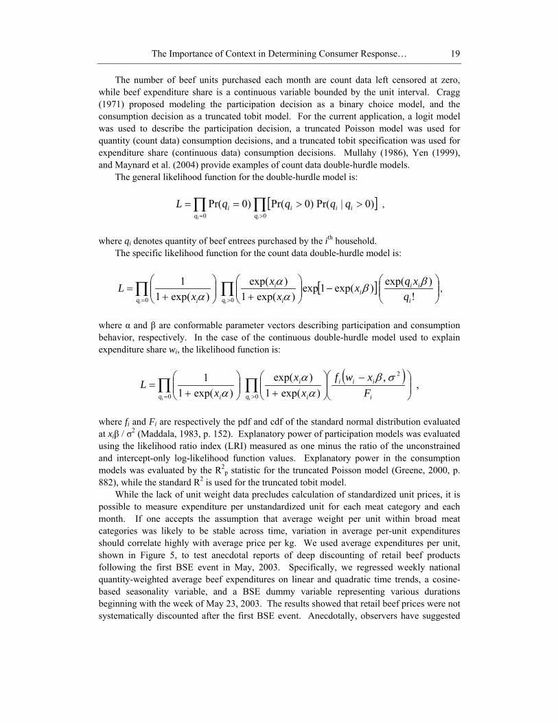
While the lack of unit weight data precludes calculation of standardized unit prices, it ispossible to measure expenditure per unstandardized unit for each meat category and eachmonth. If one accepts the assumption that average weight per unit within broad meatcategories was likely to be stable across time, variation in average per-unit expendituresshould correlate highly with average price per kg. We used average expenditures per unit,shown in Figure 5, to test anecdotal reports of deep discounting of retail beef productsfollowing the first BSE event in May, 2003. Specifically, we regressed weekly nationalquantity-weighted average beef expenditures on linear and quadratic time trends, a cosine-based seasonality variable, and a BSE dummy variable representing various durationsbeginning with the week of May 23, 2003. The results showed that retail beef prices were notsystematically discounted after the first BSE event. Anecdotally, observers have suggested
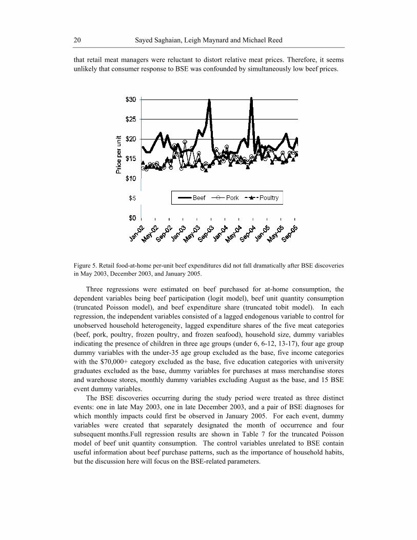
Sayed Saghaian, Leigh Maynard and Michael Reed20
that retail meat managers were reluctant to distort relative meat prices. Therefore, it seemsunlikely that consumer response to BSE was confounded by simultaneously low beef prices.
Figure 5. Retail food-at-home per-unit beef expenditures did not fall dramatically after BSE discoveriesin May 2003, December 2003, and January 2005.
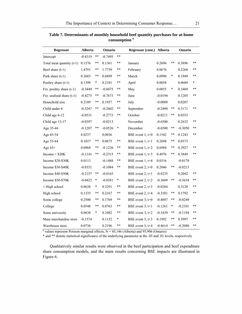
Three regressions were estimated on beef purchased for at-home consumption, thedependent variables being beef participation (logit model), beef unit quantity consumption(truncated Poisson model), and beef expenditure share (truncated tobit model). In eachregression, the independent variables consisted of a lagged endogenous variable to control forunobserved household heterogeneity, lagged expenditure shares of the five meat categories(beef, pork, poultry, frozen poultry, and frozen seafood), household size, dummy variablesindicating the presence of children in three age groups (under 6, 6-12, 13-17), four age groupdummy variables with the under-35 age group excluded as the base, five income categorieswith the $70,000+ category excluded as the base, five education categories with universitygraduates excluded as the base, dummy variables for purchases at mass merchandise storesand warehouse stores, monthly dummy variables excluding August as the base, and 15 BSEevent dummy variables.
The BSE discoveries occurring during the study period were treated as three distinctevents: one in late May 2003, one in late December 2003, and a pair of BSE diagnoses forwhich monthly impacts could first be observed in January 2005. For each event, dummyvariables were created that separately designated the month of occurrence and foursubsequent months.Full regression results are shown in Table 7 for the truncated Poissonmodel of beef unit quantity consumption. The control variables unrelated to BSE containuseful information about beef purchase patterns, such as the importance of household habits,but the discussion here will focus on the BSE-related parameters.
The Importance of Context in Determining Consumer Response… 21
Table 7. Determinants of monthly household beef quantity purchases for at-homeconsumption a
Regressor Alberta Ontario Regressor (cont.) Alberta Ontario
Intercept -0.4319 ** -0.7495 **
Total meat quantity (t-1) 0.1576 ** 0.1361 ** January 0.2696 ** 0.3896 **
Beef share (t-1) 1.4791 ** 1.7739 ** February 0.0676 0.2268 **
Pork share (t-1) 0.3603 ** 0.6899 ** March 0.0990 * 0.1949 **
Poultry share (t-1) 0.1399 * 0.2181 ** April 0.0058 0.0689 *
Frz. poultry share (t-1) -0.3449 ** -0.6075 ** May 0.0855 * 0.3469 **
Frz. seafood share (t-1) -0.4275 ** -0.7673 ** June -0.0194 0.1205 **
Household size 0.2189 ** 0.1957 ** July -0.0009 0.0207
Child under 6 -0.3247 ** -0.2602 ** September -0.2498 ** 0.3171 **
Child age 6-12 -0.0531 -0.2773 ** October -0.0211 ** 0.0353
Child age 13-17 -0.0397 -0.0213 November -0.6500 0.2632 **
Age 35-44 -0.1207 ** -0.0526 * December -0.6500 ** -0.3050 **
Age 45-54 0.0237 0.0036 BSE event 1, t+0 0.1542 ** 0.1243 **
Age 55-64 0.1037 ** 0.0875 ** BSE event 1, t+1 0.2698 ** 0.0573
Age 65+ 0.0968 ** -0.1226 ** BSE event 1, t+2 0.6984 ** 0.3927 **
Income < $20K -0.1141 ** -0.2315 ** BSE event 1, t+3 0.4976 ** 0.3849 **
Income $20-$30K 0.0113 -0.1488 ** BSE event 1, t+4 0.0316 -0.0178
Income $30-$40K -0.0331 -0.1084 ** BSE event 2, t+0 0.2046 ** -0.0213
Income $40-$50K -0.2157 ** -0.0165 BSE event 2, t+1 -0.0235 0.2042 **
Income $50-$70K -0.0422 * -0.0281 * BSE event 2, t+2 -0.3609 ** -0.3634 **
< High school 0.0638 * 0.3291 ** BSE event 2, t+3 -0.0284 0.3120 **
High school 0.1335 ** 0.2167 ** BSE event 2, t+4 -0.3381 ** 0.1792 **
Some college 0.2500 ** 0.1769 ** BSE event 3, t+0 -0.4887 ** -0.0249
College 0.0548 ** 0.0763 ** BSE event 3, t+1 -0.1261 * -0.2101 **
Some university 0.0638 * 0.1082 ** BSE event 3, t+2 -0.3439 ** -0.1194 **
Mass merchandise store -0.1574 0.1152 * BSE event 3, t+3 0.1992 ** 0.3997 **
Warehouse store 0.0736 0.2196 ** BSE event 3, t+4 -0.4614 ** -0.2080 **a values represent Poisson marginal effects, N = 45,146 (Alberta) and 95,906 (Ontario)* and ** denote statistical significance of the underlying parameter at the .05 and .01 levels, respectively
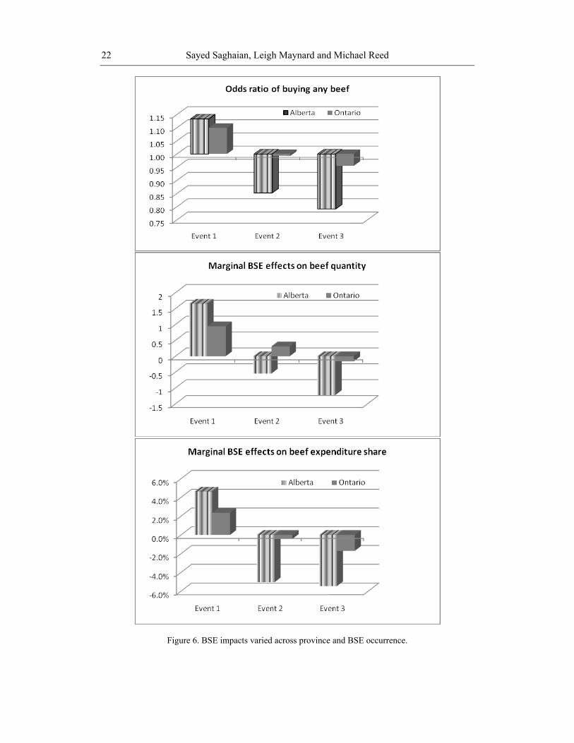
Qualitatively similar results were observed in the beef participation and beef expenditureshare consumption models, and the main results concerning BSE impacts are illustrated inFigure 6.
Sayed Saghaian, Leigh Maynard and Michael Reed22
Figure 6. BSE impacts varied across province and BSE occurrence.

The Importance of Context in Determining Consumer Response… 23
One of the main results, and an unexpected one, is that consumers reacted to the first BSEevent by significantly increasing beef purchases. Increases were observed in all measures:likelihood of buying beef, quantity of beef units purchased, and beef expenditure sharerelative to other meats. Comparing the magnitude of quantity marginal effects in Table 7(e.g., 0.15 to 0.70 units in Alberta) to average monthly purchase quantities (e.g., 2.13 units inAlberta), the results suggest economically significant increases in beef purchases attributableto the first BSE event. Positive impacts were stronger and more immediate in Alberta than inOntario, perhaps reflecting Albertans’ proximity to the struggling ranching sector. Combinedwith Boyd and Jardine’s (2007) findings that media coverage following the first BSE eventemphasized trade impacts over food safety concerns, our results suggest that many Canadiansinitially rallied to support ranchers.
Consumer perception appeared to change following the second and third BSE events,with negative impacts dominating. As with the first event, the impacts were statistically andeconomically significant and substantially stronger in Alberta than in Ontario. The resultssuggest that food safety fears began to mount as multiple cases of BSE were discovered. Adetailed analysis of media coverage following the second and third events has not yet beenperformed. Given the active involvement of government agencies’ in supplying publicinformation about BSE, sometimes in concert with beef industry organizations, it would bepolicy-relevant to test if the nature of media coverage correlated highly with consumerresponses. Overall, the results demonstrate a need to evaluate BSE events individually, ratherthan measuring an average or net consumer response to BSE.
Canadian BSE Impacts on Food-away-from-Home Beef Purchases
The possibility exists that BSE concerns were expressed more strongly in food away-from-home purchases, where consumers delegate food sourcing and preparation torestaurants. Consumers receive little information about the safety of beef purchased inrestaurants. Fast food beef purchases are of special interest due to the prominence of groundbeef products, which are the most likely vehicle for BSE-infected nerve tissue.
Building on the context-dependent results of the food-at-home analysis described above,this section reports an extension of an analysis by Maynard, Goddard, and Conley (2008).The original analysis evaluated average responses to BSE media coverage in Alberta andOntario, while the present analysis uses nationwide data and evaluates responses specific toeach BSE discovery.
The analysis was performed on the NPD Group, Inc. Consumer Report on Eating ShareTrends (CREST) dataset describing Canadian food away-from-home purchases for the periodfrom May, 2000 to May, 2005. The dataset was purchased by the Consumer and MarketDemand Agricultural Policy Research Network, and contains individual meal records fromapproximately 4,000 households per quarter. We restricted our attention to non-breakfast,fast food purchases, and aggregated each household’s purchases by month, producing 44,246observations.
Variables include a household ID number, codes for up to eight items purchased by eachindividual, the price paid by the entire party, a wide range of socio-economic anddemographic variables describing households and individual diners, and detailed data on thetime, location, and context of each meal. Table 8 shows descriptive statistics of variables

Sayed Saghaian, Leigh Maynard and Michael Reed24
used in the analysis. Specific food codes were categorized into 23 subcategories, of which 14referred to entrées. Following estimation of entrée unit prices (described below), the entréesubcategories were further aggregated into beef, chicken, pizza, and “other” designations foruse in the primary analysis. Beef entrees such as hamburgers were the most commonlyreported and most numerous entrée, followed closely by chicken.
Table 8. Descriptive Statistics of Canadian Fast Food Purchases, May 2000 – May 2005
Mean Std. Dev.Beef entree (0/1) 0.37 0.48Chicken entree (0/1) 0.34 0.47Pizza entree (0/1) 0.28 0.45Other entree (0/1) 0.44 0.50Number of beef entrees 1.10 1.79Number of chicken entrees 0.75 1.47Number of pizza entrees 0.74 1.54Number of other entrees 0.98 1.62Promotional deal (0/1) 0.37 0.43Price of beef entrée ($) 2.83 0.42Price of chicken entrée ($) 3.42 0.48Price of pizza entrée ($) 5.49 0.52Price of other entrée ($) 4.20 0.31Age of household head 48.23 14.31Married (0/1) 0.69 0.46Children (0/1) 0.36 0.48College degree (0/1) 0.28 0.45Female head works full time (0/1) 0.36 0.48English second language (0/1) 0.26 0.44Restaurant within 5 minutes (0/1) 0.47 0.44Came from work (0/1) 0.20 0.35Came from home (0/1) 0.33 0.41
N = 44,246, where each observation represents a household's purchases in a given month
As in the preceding analysis of beef purchased for at-home consumption, a double-hurdlemodel was used to distinguish between participation and consumption decisions. Thedetailed data set offered dozens of potential regressors. Consumer demand theory suggestedthe inclusion of several variables in the double-hurdle model, and other variables wereincluded when they correlated highly with beef entrée purchases and did not induce severemulticollinearity. Variables relating to the household head refer to the female household headwhen both genders were present.
Following Maynard, Goddard, and Conley (2008), the dependent variable in theparticipation model was a dummy variable for beef entrée purchases, and in the consumptionmodel the dependent variable was the number of beef entrées purchased by a given householdin a given month. Regarding independent variables, a dummy variable called “promotionaldeal” indicated meals purchased under a special price, coupon, or other offer. Demographicvariables included the age of the household head, whether the household heads were married,whether children under age 18 lived in the household, whether the household head had a
The Importance of Context in Determining Consumer Response… 25
university degree, whether the female household head worked full time outside the home, andwhether English was a second language for the household head. Travel time to the restaurantand the diner’s location prior to the meal were included as regressors. As in the Canadianfood-at-home analysis, household habits were controlled using the most recent laggeddependent variables.
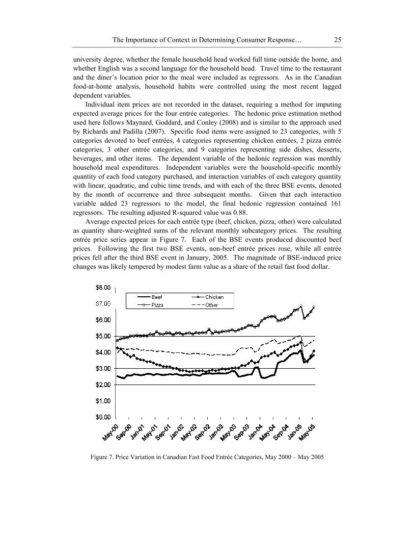
Individual item prices are not recorded in the dataset, requiring a method for imputingexpected average prices for the four entrée categories. The hedonic price estimation methodused here follows Maynard, Goddard, and Conley (2008) and is similar to the approach usedby Richards and Padilla (2007). Specific food items were assigned to 23 categories, with 5categories devoted to beef entrées, 4 categories representing chicken entrées, 2 pizza entréecategories, 3 other entrée categories, and 9 categories representing side dishes, desserts,beverages, and other items. The dependent variable of the hedonic regression was monthlyhousehold meal expenditures. Independent variables were the household-specific monthlyquantity of each food category purchased, and interaction variables of each category quantitywith linear, quadratic, and cubic time trends, and with each of the three BSE events, denotedby the month of occurrence and three subsequent months. Given that each interactionvariable added 23 regressors to the model, the final hedonic regression contained 161regressors. The resulting adjusted R-squared value was 0.88.
Average expected prices for each entrée type (beef, chicken, pizza, other) were calculatedas quantity share-weighted sums of the relevant monthly subcategory prices. The resultingentrée price series appear in Figure 7. Each of the BSE events produced discounted beefprices. Following the first two BSE events, non-beef entrée prices rose, while all entréeprices fell after the third BSE event in January, 2005. The magnitude of BSE-induced pricechanges was likely tempered by modest farm value as a share of the retail fast food dollar.
Figure 7. Price Variation in Canadian Fast Food Entrée Categories, May 2000 – May 2005
Sayed Saghaian, Leigh Maynard and Michael Reed26
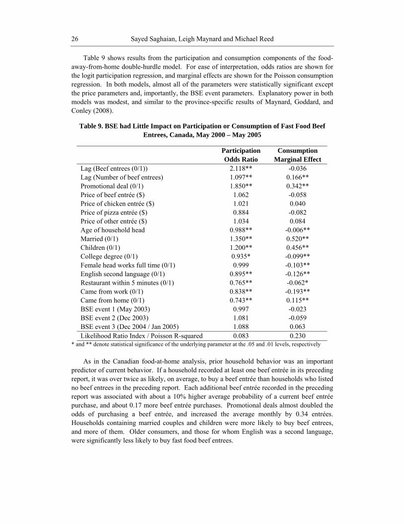
Table 9 shows results from the participation and consumption components of the food-away-from-home double-hurdle model. For ease of interpretation, odds ratios are shown forthe logit participation regression, and marginal effects are shown for the Poisson consumptionregression. In both models, almost all of the parameters were statistically significant exceptthe price parameters and, importantly, the BSE event parameters. Explanatory power in bothmodels was modest, and similar to the province-specific results of Maynard, Goddard, andConley (2008).
Table 9. BSE had Little Impact on Participation or Consumption of Fast Food BeefEntrees, Canada, May 2000 – May 2005
ParticipationOdds Ratio
ConsumptionMarginal Effect
Lag (Beef entrees (0/1)) 2.118** -0.036Lag (Number of beef entrees) 1.097** 0.166**Promotional deal (0/1) 1.850** 0.342**Price of beef entrée ($) 1.062 -0.058Price of chicken entrée ($) 1.021 0.040Price of pizza entrée ($) 0.884 -0.082Price of other entrée ($) 1.034 0.084Age of household head 0.988** -0.006**Married (0/1) 1.350** 0.520**Children (0/1) 1.200** 0.456**College degree (0/1) 0.935* -0.099**Female head works full time (0/1) 0.999 -0.103**English second language (0/1) 0.895** -0.126**Restaurant within 5 minutes (0/1) 0.765** -0.062*Came from work (0/1) 0.838** -0.193**Came from home (0/1) 0.743** 0.115**BSE event 1 (May 2003) 0.997 -0.023BSE event 2 (Dec 2003) 1.081 -0.059BSE event 3 (Dec 2004 / Jan 2005) 1.088 0.063Likelihood Ratio Index / Poisson R-squared 0.083 0.230
* and ** denote statistical significance of the underlying parameter at the .05 and .01 levels, respectively
As in the Canadian food-at-home analysis, prior household behavior was an importantpredictor of current behavior. If a household recorded at least one beef entrée in its precedingreport, it was over twice as likely, on average, to buy a beef entrée than households who listedno beef entrees in the preceding report. Each additional beef entrée recorded in the precedingreport was associated with about a 10% higher average probability of a current beef entréepurchase, and about 0.17 more beef entrée purchases. Promotional deals almost doubled theodds of purchasing a beef entrée, and increased the average monthly by 0.34 entrées.Households containing married couples and children were more likely to buy beef entrees,and more of them. Older consumers, and those for whom English was a second language,were significantly less likely to buy fast food beef entrees.

The Importance of Context in Determining Consumer Response… 27
The finding that prices were not significant determinants of beef entrée purchases is notentirely surprising when considering the context of fast food purchases. As shown in Figure7, the relative ordering of fast food entrée prices is stable over time, i.e., beef products aregenerally less expensive than chicken products, which in turn are less expensive than pizza.Awareness of typical fast food prices is likely to be high among most consumers, and fewlower-cost, low-preparation alternatives are available. Convenience and product attributepreferences are likely to be among the most important demand determinants.
The failure of BSE events to influence the likelihood or quantity of beef entrée purchasesis more surprising, as it conflicts with the statistically and economically significant impactsfrom the food-at-home analysis. The results correspond roughly with those of Maynard,Goddard, and Conley (2008), who found limited evidence that BSE media coverage affectedthe likelihood of purchasing fast food beef entrees, but not the quantity, among Ontarioconsumers. Based on the food-at-home results, we hypothesized that distinguishing amongBSE events would also be important in the fast food context, but the results do not supportthis hypothesis, or challenge the validity of the undifferentiated media index used byMaynard, Goddard, and Conley (2008). The results also fail to support the hypothesis thatconsumers would perceive greater food safety threats from fast food beef products than frombeef products purchased for at-home consumption.
The two Canadian analyses presented here were each based on extremely large samplesthat appeared to be demographically representative of Canada’s general population, based on2001 Census figures (Statistics Canada, 2006b). It is therefore interesting that responses toBSE would be so different across the food-at-home and food-away-from-home venues.Given the prominence of food safety issues in recent regulatory and trade policy debates,exploring the reasons for divergent behavior across market venues is a useful topic for furtherstudy.
Summary
In the first section, we examined the impact of two beef safety scares on retail-level percapita meat consumption and prices in Japan. The objective was to investigate Japaneseconsumer reactions to the news of BSE discoveries at the retail level to better understandconsumer responses to beef safety scares, and help the industry restore consumer confidenceafter food safety crises. This in turn, provides opportunities for national-level productdifferentiation based on beef quality and traceability.
Consumers account for the nature of the contamination and respond to informationregarding the origin and type of contaminated beef products with their purchasing decisions.Beef exporters and producer groups can use the study’s findings as a rationale for effectiveand transparent communication with consumers, and provide credible quality assurances. Thefindings emphasize the need for beef industry representatives to be immediately involved inproviding accurate information when a safety crisis arises. Consumers consider food safetyan entitlement, and most are unlikely to pay large premiums for safety assurance unless crisesare frequent or locally prominent. Credible efforts that raise consumer confidence in an entirenation’s beef supply may be justified in order to reduce erosion of demand and market sharewhen safety crises do occur.

Sayed Saghaian, Leigh Maynard and Michael Reed28
In the second part of this study, we addressed the dynamic impact of the 2003 BSEdiscovery on the U.S. beef sector. Time-series analysis and historical decomposition ofweekly feedlot, wholesale, and retail beef prices were used to address the dynamics of priceadjustment and causality along the U.S. beef marketing channel. The results showed that pricetransmission was bi-directional, determined through interaction between the different stages,and price adjustment was asymmetric with respect to speed and magnitude. The resultsrevealed a differential impact of the exogenous shock on producers and retailers, leading towidening of price margins and pointing to imperfect price transmission, specifically at theretail level, which could have consequences for the efficiency and equity of the U.S. beefmarketing channel.
In the third part, two large, household-level datasets were used to evaluate the impact ofBSE on retail beef purchases in grocery stores and fast food restaurants. Each datasetencompassed the first four Canadian-born cases of BSE, occurring between May, 2003 andJanuary, 2005. Double-hurdle models were estimated to identify BSE impacts onhouseholds’ monthly probability of purchasing beef, and monthly frequency, quantity, and/orexpenditure share of beef purchases. Consumers in Alberta and Ontario purchased more beeffollowing the initial BSE discovery, even after controlling for other factors, but respondednegatively to subsequent BSE events. Consumer response was stronger in Alberta than inOntario. BSE did not appear to systematically affect Canadian fast food beef purchases.
References
Agriculture and Livestock Industries Corporations (ALIC). ALIC Monthly Statistics. Tokyo,ALIC, Various Issues, 1994-2002.
Babula, R., Bessler, D., & Payne, W. (2004). Dynamic relationships among U.S. wheat-related markets: Applying directed acylic graphs to a time series model. Journal ofAgricultural and Applied Economics, 36, 1, 1-22.
Baker, G.A. (1998). “Strategic implications of consumer food safety preferences.”International Food and Agribusiness Management Review, 1, 4, 451-463.
Bakucs, L.Z. & Ferto, I. (2005). Marketing margins and price transmission on the Hungarianpork meat market. Agribusiness, 21, 2, 273-286.
Becker, T., Benner, E. and Glitsch, K. (1996). Wandel des Verbraucherverhatens bei Fleisch.Agrarwirtschaft, 45, 267-277.
Ben-Kaabia, M, Gill, J.M., & Boshnjaku, L. (2002). Price transmission asymmetries in theSpanish lamb sector. Paper presented at the X. Congress of European Association ofAgricultural Economists, Zaragoza, Spain, 28-31, August.
Bessler, D.A. & Akleman, D.G. (1998). “Farm prices, retail prices and directed graphs:Results for pork and beef.” American Journal of Agricultural Economics, 80, 1144-1149.
Bocker, A. (2002). Consumer response to a food safety incident: exploring the role ofsupplier differentiation in an experimental study. European Review of AgriculturalEconomics, 29, 1, 29-50.
Bocker, A. & Hanf, C.-H. (2000). Confidence lost—partially—regained: consumers’response to food scares. Journal of Economic Behavior and Organization, 43, 471-485.
Bordo, M. D. (1980). The effects of monetary change on relative commodity prices and therole of long-term contracts.” Journal of Political Economy, 88, 6, 1088-1109.
The Importance of Context in Determining Consumer Response… 29
Boyd, A.D. and C.G. Jardine. (2007). Public risk perceptions of BSE and vCJD: An Albertanperspective. Presented at the meetings of the Agricultural Institute of Canada, Edmonton,Alberta.
Brown, D.J. and L.F. Schrader. (1990). Cholesterol information and shell egg consumption.American Journal of Agriculture Economics 72: 548-555.
Burton, M., R. Dorsett, and T. Young. (1996). Changing preferences for meat: evidence fromUK household data, 1973-93. European Review of Agricultural Economics 23: 357-370.
Burton, M. and T. Young. (1996). The impact of BSE on the demand for beef and other meatsin Great Britain. Applied Economics 28: 687-693.
Cameron, A.C. and P.K. Trivedi. (1986). Econometric models based on count data:comparisons and applications of some estimators and tests. Journal of AppliedEconometrics 1:29-53.
Chopra, A. & Bessler, D.A. (2005). “Impact of BSE and FMD on beef industry in U.K.”Paper presented at the NCR-134 Conference on Applied Commodity Price Analysis,Forecasting, and Market Risk Management, St. Louis, Missouri, April 18-19.
Cragg, J.G. (1971). Some statistical models for limited dependent variables with applicationto the demand for durable goods. Econometrica 39:829-844.
de Jonge, J., H. van Trijp, E. Goddard, and L. Frewer. (2006). The reciprocal relationshipbetween public policy making and consumer confidence in food safety: a cross-nationalperspective. working paper, Wageningen University, Marketing and ConsumerBehaviour Group.
Fearne, A., Hornibrook, S. & Dedman S. (2001). “The management of perceived risk in thefood supply chain: A comparative study of retailer-led beef quality assurance schemes inGermany and Italy.” Imperial College at Wye Research Paper. University of London,Wye, Ashford, Kent. TN255AH.
Fox, J.A. & Peterson, H.H. (2002). “Bovine Spongiform Encephalopathy (BSE): Risk andimplications for the United States.” Paper presented at the NCR-134 Conference onApplied Commodity Price Analysis, Forecasting, and Market Risk Management, St.Louis, MO, April, 22-23.
Gardner, B.L. (1975). The farm-retail spread in a competitive food industry. AmericanJournal of Agricultural Economics, 57, 399-409.
Goodwin, B.K. & Harper, D.C. (2000). Price transmission, threshold behavior, andasymmetric adjustment in the U.S. pork sector. Journal of Agricultural and AppliedEconomics, 32, 3, 543-553.
Goodwin, B.K. & Holt, M.T. (1999). Price transmission and asymmetric adjustment in TheU.S. beef sector. American Journal of Agricultural Economics, 81, 3, 630-637.
Greene, W.H. 2000. Econometric Analysis, 4th Edition. Upper Saddle River, N.J.: PrenticeHall.
Heien, D.M. (1980). Markup pricing in a dynamic model of the food industry. AmericanJournal of Agricultural Economics, 62, 10-18.
Hicks, J. (1974). The crisis in Keynesian economics. Basic Books, New York.Johansen, S., & Juselius, K. (1992). “Testing structural hypothesis in a multivariate co-
integration analysis of the PPP and UIP for the UK.” Journal of Econometrics, 53, 211-244.
Sayed Saghaian, Leigh Maynard and Michael Reed30
Livanis, G. & Moss, C.B. (2005). “Price transmission and food scares in the U.S. beefsector.” Paper presented at the American Agricultural Economics Association Meetings,Providence, RI.
Lloyd, T., McCorriston, S., Morgan, W., & Rayner, T. (2003) Food scares, market power andrelative price adjustment in the UK. Discussion Papers in Economics, University ofNottingham, Discussion Paper No. 03/18.
Luoma, A., Luoto, J. & Taipale, M. (2004). Threshold cointegration and asymmetric pricetransmission in Finish beef and pork markets. Pellervo Economic Research Instituteworking paper No. 70, November.
Maddala, G.S. 1983. Limited-Dependent and Qualitative Variables in Econometrics.Cambridge, U.K.: Cambridge University Press.
Marsh, T.L., Schroeder, T.C. & Mintert, J. (2004). “Impacts of meat product recalls onconsumer demand in the USA.” Applied Economics, 36, 897-909.
Maynard, L.J., E. Goddard, and J. Conley. (2008). Impact of BSE on Beef Purchases inAlberta and Ontario Quick-Serve Restaurants. Canadian Journal of AgriculturalEconomics 55,3: forthcoming.
Maynard, L.J., J.G. Hartell, A.L. Meyer, and J. Hao. (2004). An experimental approach tovaluing new differentiated products. Agricultural Economics, 31: 317-325.
Mazzocchi, M. (2005). “Modeling consumer reaction to multiple food scares.” Department ofAgricultural and Food Economics Research Paper. The University of Reading.
McCluskey, J.J., Grimsrud, K.M., Ouchi, H. & Wahl, T.I. (2004). “BSE in Japan:Consumers’ perceptions and willingness to pay for tested beef.” Washington StateUniversity Research Paper, TWP-111.Miller, J.D. & Hayenga, M.L. (2001). Price cyclesand asymmetric price transmission in the U.S. pork market. American Journal ofAgricultural Economics, 83,551-561.
Mullahy, J. (1986). Specification and testing of some modified count data models. J.Econometrics 33: 341-365.
NCJDSU (National Creutzfeldt-Jakob Disease Surveillance Unit). (2008). CJD Statistics.Western General Hospital, Edinburgh, Scotland.
Okun, A. (1975). Inflation: Its mechanics and welfare costs. Brooking Papers on EconomicActivity, 2, 351-390.
Paarlberg, P. L., Lee, J. G. & Seitzinger, A. H. (2003). “Measuring welfare effects of an FMDoutbreak in the United States.” Journal of Agricultural and Applied Economics, 35, 1,53-65.
Pelzman, S. (2000). Prices rise faster than they fall. Journal of Political Economy, 108, 3,446-502.
Peng, Y., D. McCann-Hiltz, and E. Goddard. (2005). Consumer demand for meat in Alberta,Canada: Impact of BSE. Presented at the 2005 meetings of the American AgriculturalEconomics Association, Denver, Co..
Peterson, H.H. & Chen, Y.J. (2005). “The impact of BSE on Japanese retail meat demand.”Agribusiness: an international journal, 21, 3, 313-327.
Piggott, N.E. & Marsh, T.L. (2004). “Does food safety information impact U.S. meatdemand?” American Journal of Agricultural Economics, 86, 154-174.
Pritchett, J. and D. Thilmany. (2005). The cow that stole Christmas? Exploring the role ofmedia coverage in recent BSE outbreaks. Western Economics Forum 4(2): 24-28.
RATS (2004) User’s Guide, version 6, Estima.

The Importance of Context in Determining Consumer Response… 31
Richard, T.J. and L. Padilla. (2007). Promotion and fast food demand: Where’s the beef?Consumer and Market Demand Agricultural Policy Research Network Project ReportCMD-07-03, Edmonton, Alberta.
Saghaian, S. (2007). “Beef Safety Shocks and Dynamics of Vertical Price Adjustment: TheCase of BSE Discovery in the U.S. Beef Sector.” Agribusiness: An International Journal,Vol. 23, Issue No. 3, 333-348.
Saghaian, S., Hasan, M.F. and Reed, M. (2002). “Overshooting of agricultural prices in fourAsian economies. Journal of Agricultural and Applied Economics, 34,1, 95-109.
Saghaian, S., Maynard, L., & Reed, M. (2007). “The effect of E. Coli 0157:H7, FMD andBSE on Japanese retail beef prices: A historical decomposition.” Agribusiness: AnInternational Journal, 23, 1, 131-147.
Saghaian, S, and Reed, M. (2007). “Consumer Reaction to Beef Safety Scares.” InternationalFood and Agribusiness Management Review, Vol. 10, Issue No. 1, 18-35.
Schmidt, M. B. (2000). “The dynamic behavior of wages and prices: Co-integration testswithin a large macroeconomic system.” Southern Economic Journal, 67, 123-138.
Spirtes, P., Scheines, R., Meek, C., Richardson, T., Glymour, C., Boomsam, A., & Hoijtink,H. (1999). TETRAD II-Version 3.1 Tools for Causal Modeling. Pittsburgh PA. CarnegieMellon University.
Spirtes, P., Glymour, C. & Scheines, R. (2000). Causation, Prediction, and Search. NewYork: Springer-Verlag.
Statistics Canada. (2006a). Canada’s beef industry and BSE. accessed October 5, 2006, Lastmodified June 28, 2006, http://www41.statcan.ca/0920/ceb0920_001_e.htm .
Statistics Canada. (2006b). 2001 Census of Canada. accessed September 21, 2006,http://www12.statcan.ca/english/census01/home/Index.cfm .
Swanson, N.R., & Granger, C.W.J. (1997). “Impulse response functions based on a causalapproach to residual orthogonalization in vector autoregressions.” Journal of AmericanStatistical Association. 92, 357-367.
Tiffin, R. & Dawson, P.J. (2000). Structural breaks, cointegration and the farm retail pricespread for lamb. Applied economics, 32,1281-1286.
Vickner, S.S., D. Bailey, and A. Dustin. (2006). Estimating the market demand for value-added beef: Testing for BSE announcement effects using a nested PIGLOG modelapproach. Presented at the 2006 meetings of the American Agricultural EconomicsAssociation, Long Beach, Ca.
Yen, S.T. (1999). Gaussian versus count-data hurdle models: Cigarette consumption bywomen in the U.S. Applied Economics Letters 6: 73-76.
Zachariasse, L.C. & Bunte, F.H.J. (2003). How are farmers faring in the changing balancedimensions of the food economy: Exploring the policy issues. Den Haag, 6-7, February.