Submitted for publication (Paper id: 226) INCOSE International Symposium, 20-23 June 2011, Denver CO, U.S.A

Satellites to Supply Chains, Energy to Finance — SLIM for Model-Based Systems Engineering

Part 2: Applications of SLIM

Copyright © 2011 InterCAX LLC and Georgia Institute of Technology. Published and used by INCOSE with permission.

Manas Bajaj1*, Dirk Zwemer1, Russell Peak2, Alex Phung1, Andrew Scott1, Miyako Wilson2

1. InterCAX LLC 75 5th Street, Suite 213, Atlanta GA 30308 USA

www.intercax.com

2. Georgia Institute of Technology Model-Based Systems Engineering Center,

MARC, 813 Ferst Drive, Atlanta GA 30318 USA www.mbse.gatech.edu

Abstract Development of complex systems is a collaborative effort spanning disciplines, teams,

processes, software tools, and modeling formalisms. Increasing system complexity, reduction in available resources, globalized and competitive supply chains, and volatile market forces necessitate that a unified model-based systems engineering environment replace ad-hoc, document-centric and point-to-point environments in organizations developing complex systems.

To address this challenge, we envision SLIM—a collaborative, model-based systems

engineering workspace for realizing next-generation complex systems. SLIM uses SysML to represent the front-end conceptual abstraction of a system that can “co-evolve” with the underlying fine-grained connections to models in discipline-specific tools and standards. With SLIM, system engineers can drive automated requirements verification, system simulations, trade studies and optimization, risk analyses, design reviews, system verification and validation, and other key systems engineering tasks from the earliest stages of development directly from the SysML-based system model. SLIM provides analysis tools that are independent of any systems engineering methodology, and integration tools that connect SysML with a wide variety of COTS and in-house design and simulation tools.

We are presenting SLIM and its applications in two papers. In Part 1 paper—Motivation and Concept of SLIM—we presented the motivation and challenges that led to SLIM, the conceptual architecture of SLIM, and SLIM tools available for production and evaluation usage. In Part 2 (this paper), we present the applications of SLIM tools to a variety of domains, both in traditional as well as non-traditional domains of systems engineering. Representative SysML models and results of trade studies, risk analysis, and other system engineering tasks performed using SLIM tools are presented for the following domains—space systems, energy systems, infrastructure systems, manufacturing and supply chain systems, military operations, and bank systems.

* Corresponding author: Manas Bajaj, manas.bajaj@intercax.com, phone: +1-404-592-6897. Preferred citation:

Bajaj, M., Zwemer, D., Peak, R., Phung, A., Scott, A. and Wilson, M. (2011). Satellites to Supply Chains, Energy to Finance — SLIM for Model-Based Systems Engineering, Part 1: Motivation and Concept of SLIM. 21st Annual INCOSE International Symposium, Denver, CO, June 20-23, 2011.

1

1 Introduction In this paper, we present applications of SLIM for model-based systems engineering in a

variety of domains (Sections 2-7). For each domain we present an overview of the representative SysML model, the analyses performed using SLIM tools, and the results of analyses. These SysML models are extensive but not all diagrams or details are presented in this paper. The purpose of the models and the analyses presented in this paper is to introduce the reader to the application of SysML and SLIM tools in these traditional and non-traditional domains of systems engineering.

2 Space Systems The application of model-based systems engineering to space systems is growing. In this

section, we present the application of SLIM tools to the space system domain using the FireSat model being developed as part of the INCOSE Space Systems Working Group challenge team. Figure 1 below shows a SysML block definition diagram of the FireSat domain. Development of complex space systems requires modeling not only the spacecraft but the mission and the supporting systems that influence the design and operation of the spacecraft. As shown in the figure, this includes the ground station, communication networks, space mission, and even celestial bodies such as the Earth and Sun.

Figure 1: Block definition diagram for the FireSat domain

2

The objective of a FireSat satellite is to detect forest fires on Earth and communicate information to the ground station which can forward this to local emergency services for timely rescue and response. Figure 2 shows a SysML parametric model that is used to compute the performance metrics (daily coverage, resolution), and the annual operating cost of a FireSat satellite from its design and operational parameters. The performance metrics and the cost variable are highlighted in red in the parametric diagram. The parametric model also shows constraints to verify requirements. The ResolutionReqt constraint block is used for the rR1 constraint property (bottom right corner of the parametric diagram) and is a mathematical representation of a text-based requirement concerning FireSat scan resolution. It compares the scan resolution to the required value (30m) and computes the ScanResVerify property that represents the result of verifying the resolution requirement (1 for pass and 0 for fail).

Figure 2: SysML parametric model for computing coverage, scan resolution, and flight cost of the FireSat Figure 3 and Figure 4 show the results of a trade study and requirement verification conducted using ParaMagic®—Parametric solver tool for MagicDraw—for 1 and 2 FireSats respectively. The rows correspond to trade study scenarios, while the columns correspond to the key variables computed and verified against requirements in these trade studies. Cells highlighted in red in Figure 3 and Figure 4 indicate requirements that failed for specific scenarios. The cost requirement fails if a FireSat operates at lower altitudes, while the resolution requirement fails when it operates at higher altitudes. The coverage requirement failed for all scenarios with 1 FireSat (Figure 3). The green-colored rows in Figure 4 indicate all scenarios for which all three requirements passed.

3

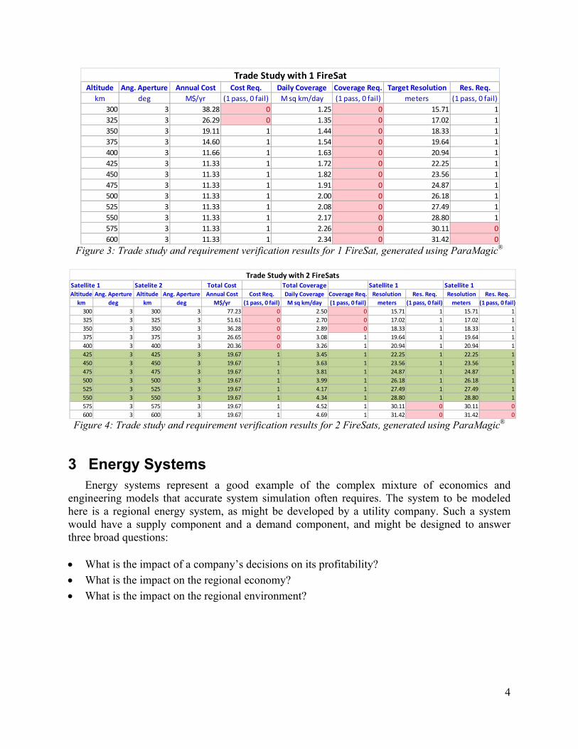
Figure 3: Trade study and requirement verification results for 1 FireSat, generated using ParaMagic®

Altitude Ang. Aperture Annual Cost Cost Req. Daily Coverage Coverage Req. Target Resolution Res. Req.km deg M$/yr (1 pass, 0 fail) M sq km/day (1 pass, 0 fail) meters (1 pass, 0 fail)

300 3 38.28 0 1.25 0 15.71 1325 3 26.29 0 1.35 0 17.02 1350 3 19.11 1 1.44 0 18.33 1375 3 14.60 1 1.54 0 19.64 1400 3 11.66 1 1.63 0 20.94 1425 3 11.33 1 1.72 0 22.25 1450 3 11.33 1 1.82 0 23.56 1475 3 11.33 1 1.91 0 24.87 1500 3 11.33 1 2.00 0 26.18 1525 3 11.33 1 2.08 0 27.49 1550 3 11.33 1 2.17 0 28.80 1575 3 11.33 1 2.26 0 30.11 0600 3 11.33 1 2.34 0 31.42 0

Trade Study with 1 FireSat

Figure 4: Trade study and requirement verification results for 2 FireSats, generated using ParaMagic®

Satellite 1 Total Cost Total CoverageAltitude Ang. Aperture Altitude Ang. Aperture Annual Cost Cost Req. Daily Coverage Coverage Req. Resolution Res. Req. Resolution Res. Req.

km deg km deg M$/yr (1 pass, 0 fail) M sq km/day (1 pass, 0 fail) meters (1 pass, 0 fail) meters (1 pass, 0 fail)300 3 300 3 77.23 0 2.50 0 15.71 1 15.71 1325 3 325 3 51.61 0 2.70 0 17.02 1 17.02 1350 3 350 3 36.28 0 2.89 0 18.33 1 18.33 1375 3 375 3 26.65 0 3.08 1 19.64 1 19.64 1400 3 400 3 20.36 0 3.26 1 20.94 1 20.94 1425 3 425 3 19.67 1 3.45 1 22.25 1 22.25 1450 3 450 3 19.67 1 3.63 1 23.56 1 23.56 1475 3 475 3 19.67 1 3.81 1 24.87 1 24.87 1500 3 500 3 19.67 1 3.99 1 26.18 1 26.18 1525 3 525 3 19.67 1 4.17 1 27.49 1 27.49 1550 3 550 3 19.67 1 4.34 1 28.80 1 28.80 1575 3 575 3 19.67 1 4.52 1 30.11 0 30.11 0600 3 600 3 19.67 1 4.69 1 31.42 0 31.42 0

Trade Study with 2 FireSatsSatelite 2 Satellite 1 Satellite 1

3 Energy Systems Energy systems represent a good example of the complex mixture of economics and

engineering models that accurate system simulation often requires. The system to be modeled here is a regional energy system, as might be developed by a utility company. Such a system would have a supply component and a demand component, and might be designed to answer three broad questions:

• What is the impact of a company’s decisions on its profitability? • What is the impact on the regional economy? • What is the impact on the regional environment?

4

Figure 5: Block definition diagram (partial) showing the Regional Energy Model

In our example, detailed models are packaged as MATLAB functions. In addition to wrapping these functions as SysML constraint blocks, certain properties, including price, cost, environmental cost, supply and demand, must be rolled up from lower to higher levels of the system model and exchanged between models via parametric relationships. The SysML block definition diagram containing all the major elements is shown in Figure 5.

Parametric models capture relationships between properties of the structural elements of a SysML model. In this example, we use these relationships (constraints) in three ways:

• To wrap external models (MATLAB functions) • To capture equation-based relationships between properties • To share properties between models

Figure 6 shows an example of the first type. The constraint property EnIM1:EnvirImpact contains the constraint

envimp = xfwExternal(matlab, function, environimpact, p, ec)

5

which calls the MATLAB function “environimpact.m” with input arguments p and ec that match the function inputs and returns a value for the environmental impact. Other legacy MATLAB models are treated in the same way.

Figure 6: Energy Model parametric diagram – external MATLAB function call

Finally, some parametric diagrams show how models are tied together through equalities. The parametric diagram in Figure 7 belongs to the top level block, Regional Energy Model. The properties of this block, shown at the bottom, are tied to equivalent properties in the Profitability, Economic Impact and Environmental Impact sub-models. For example, the property Supply, which is calculated in the Regional Energy Supply block, is tied to Supply in the Regional Energy Model (not shown), where it is further tied to Supply in the other sub-models, where it is used as an input for calculating profitability, economic impact, and so forth. This is not the only way to organize the model, but it helps keep the different sub-models more modular.

Figure 7: Parametric model relating properties of environmental, economic, and profitability models

6

Our instance model of the energy system contains three generating plants: Coal, Nuclear, and Solar. With SLIM’s Parametric solver, we can explore the impact of choice in the energy mix by performing trades studies using the parametric models shown above. Reducing output increases cost on a per kW-hr basis (because fixed and capacity costs are spread over a smaller base). Increased cost and price reduce demand and system profitability. All these factors have a negative impact on the local economy. However, as shown in Figure 8, environmental impact is positive for reducing either coal or nuclear output (more positive for nuclear cutbacks) because these plants are assigned higher environmental costs than solar.

Figure 8: Results for trade study performed using ParaMagic® – Economic and Environmental Impact

4 Environmental Infrastructure Systems Man-made systems designed to control environmental resources, e.g. watershed management

projects, can take advantage of model-based systems engineering, where both the general principles governing the system behavior and the specific configuration of a particular installation can be captured in the same simulation model. Any particular body of water is subject to a standard set of processes (evaporation, consumption, etc.) following parametric conservation equations, as shown in Figure 9. A specific implementation of a network of water bodies and the gates that control flow between them is shown in Figure 10 (concept sketch) and Figure 11 (SysML Internal Block Diagram).

7

Figure 9: Watershed processes Figure 10: Network of water bodies and gates

Figure 11: SysML internal block diagram of the network of water bodies and gates The parametric model shown in Figure 12 captures the relationships in Figure 9. Another set

of parametric relationships is needed to link the input and output flows of the elements in Figure 10. A final set of parametric relationships for the gates holds the control algorithm the watershed managers will use to regulate flows through the gates. When these are completed, the SysML model can simulate the changes in water height over time for the control algorithm chosen.

8

Figure 12: SysML parametric diagram (single channel), representing the math relationships in Figure 9

5 Military Operations While modeling languages such as DoDAF and UPDM (the UML profile that supports

DoDAF) are valuable for high-level descriptions of defense system architectures, simulation of specific operational scenarios may be more easily done with SysML parametrics. In this example, a defense system based on UAV detection of time-sensitive threats such as mobile missile launchers was modeled in both UPDM and SysML. The high-level UPDM OV-1 diagram of the system is shown in Figure 13.

9

Figure 13: UPDM OV-1 diagram

Figure 14: Block definition diagram for LittleEyeMC model in Rational Rhapsody Specific elements in one scenario, detection by the LittleEye UAV and attack by joint

land/air forces is captured in the SysML block definition diagram in Figure 14. The objective of this simulation is to calculate 1) the probability that the missile launcher will fire a missile before being destroyed and 2) the probability that the missile launcher will be destroyed. The success of the defense, in this model, depends on response time and reaching the launcher before it fires a missile or returns to concealment.

10

Figure 15: Parametric diagram for Mission block in Rational Rhapsody

The response time is the sum of: 1. UAV detection time, which depends on the number of UAVs deployed 2. Intelligence analysis plus command decision time 3. Special Forces and F-18 travel time to launch site, which depends on the number of each

deployed.

Performance is not only a function of system architecture; it is also a function of resources. The high level parametric diagram for this model is shown in Figure 15. For our example, we will choose four input variables:

• MinFiringTime (TST) • MaxFiringTime (TST) • StdDetectionTime (GlobalHawk) • StdTravelTime (SpecialForces)

11

The first two capture uncertainty in the time behavior of the threat. The last two reflect location uncertainty, i.e. how far the UAV or troops must travel to reach the threat. The output variables are

• ResponseTime • ProbabilityMissileFired • ProbabilityTargetDestroyed

We set up and run a Monte Carlo study using Melody™—SLIM’s Parametric solver for Rational Rhapsody. We will assume each of the input variables follows a normal distribution with a given mean and standard deviation. Results generated by Melody for this example are shown in Figure 16. The blue bars of the histogram plot show the Response Time mean value a little over 3.5 hours. The mean probability of the missile being fired by the TST is computed as 0.9 and of the TST being destroyed is 0.78, as reported in Figure 16.

Figure 16: Histogram plot of response time from Monte Carlo simulation performed using Melody™

6 Manufacturing Systems and Supply Chains Classically, systems engineers have studied manufacturing, considered mainly as vertically

integrated factories. Increasingly, manufacturing relies on supply chains, often global in scope, and the need for models that can respond to rapidly changing customer demand, part availability and transport capacity is critical. The SysML supply chain model that we have created is shown, in a block definition diagram, in Figure 17.

12

The supply chain includes the central Company that is driving the model, the “manufacturer” as well as its customers, suppliers and transportation channels. The Company has both final production sites (install sites) and subassembly sites. Many of the composition relationship arrows are labeled with 1..*, multiplicity one to many, which is a powerful feature of SysML. It denotes that the number of elements of this type is not defined at the block definition level. The number of elements of this type is defined at the block instance level, making it easier to vary the number of suppliers, product models, projects, etc.

Figure 17: Block definition diagram of the Supply Chain system model

The goal of building this SysML model is to answer specific stakeholder questions by calculating specific properties (parameters) of the supply chain system. In our example, these properties are:

• Revenue • Value at Risk • Cost of Goods Sold (COGS) • Transportation Cost • Delay Cost

We choose to calculate these parameters by adding up these same properties at the Project

(InstallSite) level. These aggregation relationships are captured in a SysML Parametric Diagram, as shown in Figure 18. The tan boxes show the properties of the system elements, while the green boxes show the constraints or mathematical relationships between the properties. This parametric diagram shows how the total transportation cost and total cost-of-goods-sold for a company is rolled up from the transportation costs and COGS for different installation sites and

13

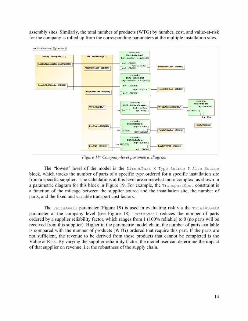
assembly sites. Similarly, the total number of products (WTG) by number, cost, and value-at-risk for the company is rolled up from the corresponding parameters at the multiple installation sites.

Figure 18: Company-level parametric diagram

The “lowest’ level of the model is the DirectPart_X_Type_Source_I_Site_Source block, which tracks the number of parts of a specific type ordered for a specific installation site from a specific supplier. The calculations at this level are somewhat more complex, as shown in a parametric diagram for this block in Figure 19. For example, the TransportCost constraint is a function of the mileage between the supplier source and the installation site, the number of parts, and the fixed and variable transport cost factors.

The PartsAvail parameter (Figure 19) is used in evaluating risk via the TotalWTGVAR

parameter at the company level (see Figure 18). PartsAvail reduces the number of parts ordered by a supplier reliability factor, which ranges from 1 (100% reliable) to 0 (no parts will be received from this supplier). Higher in the parametric model chain, the number of parts available is compared with the number of products (WTG) ordered that require this part. If the parts are not sufficient, the revenue to be derived from those products that cannot be completed is the Value at Risk. By varying the supplier reliability factor, the model user can determine the impact of that supplier on revenue, i.e. the robustness of the supply chain.

14

Figure 19: Parametric diagram to compute total number of parts, availability, part COGS, and part transportation costs for a given type of part arriving at a given installation site from multiple suppliers

Parametric calculations are performed on instances of the SysML model. An instance of the supply chain is built from a series of Excel worksheets listing the suppliers, installation sites, and subassembly sites and related data. Creating and analyzing the instance requires five steps:

1. Create an instance 2. Read supplier, part, and installation site data from Excel spreadsheets into the instance

using ParaMagic® (Excel integration tool) 3. Use ParaMagic® to execute parametric models for the instance 4. Write results from the instance to Excel spreadsheet(s) using ParaMagic® (Excel

integration tool) for reporting and visualization

Figure 20 shows sample results obtained from executing the parametric models and writing them to spreadsheets using ParaMagic®. The bar graph shows project value and cost in (thousands of dollars) for each installation site.

By adding additional parametric relationships, other questions may be answered, such as the

financial effects of local content regulations. Integration of the SysML model with an optimization engine offers the potential to rapidly realign supplier shipments in the face of market changes.

15

Figure 20: Sample results showing project value and cost by product installation sites

‐20,000 40,000 60,000 80,000 

100,000 120,000 140,000 

1 6 11 16 21 26 31

Project Value ($000)

‐

5,000 

10,000 

15,000 

20,000 

1 6 11 16 21 26 31

Project Costs ($000)Parts Cost

Tranport Cost

Delay Cost

7 Financial Risk Assessment The on-going turmoil in the world economy has highlighted the need for financial institutions

(we’ll refer to them as banks for brevity) to accurately evaluate the value and risk of their portfolios. The Basel-III Capital Accords, published in 2010, provide a framework of standards for this purpose and financial regulators in many countries are pushing their banks to report their status frequently using these standards. Given that a bank is a complex system and is part of a much larger system of markets and other institutions, SysML with parametric execution offers a promising approach to modeling institutional risk.

Risk, in a very practical sense, correlates to the level of capital reserves that an institution

must maintain to protect against negative eventualities, so it makes sense to express risk in terms of dollars (or the institution’s currency of choice). Basel-III recognizes three types of risk:

• Market Risk – the impact of reduction in equity values and/or an increase in interest rates on

the bank’s holdings. • Counterparty Risk – the impact of failure or default by an external institution (e.g. the issuer

of a bond or the other party in an option contract). • Operational Risk – the impact of all other types of negative events: government or legal

decisions, employee malfeasance, information technology failures, etc.

The evaluation of asset values, especially for the complex options and derivatives being traded today, is the core of the new field of “financial engineering”. Extremely sophisticated mathematical models have been developed to support trading desks using engineering tools like

16

MATLAB and it makes sense to integrate these pre-existing models into our SysML model for risk evaluation. In our simple example, we use some relatively simple Black-Scholes models of option pricing encapsulated as external Mathematica functions, but this principle can be extended much further.

In our example, we will be modeling the system from the bank’s point of view, i.e. the bank

at the center. See Figure 21, the high-level block definition diagram of the system.

Figure 21: SysML block definition diagram of a Bank system

Internal‐ Bank policies‐ Locations 

External Trading Partner Data‐ Assets, Debts, ExposureInternal Bank HoldingsExternal Market Data

‐ Stocks,. Bonds, Options

It may help to think about the parametric calculations in our model in two categories:

• The complex “financial engineering” calculations to evaluate the value and risk of the assets and the default probabilities of the counterparties. These are typically captured in external programs written in different computer languages and may represent core proprietary intellectual property of the bank.

• The simpler “housekeeping” calculations that, for example, sum the portfolio values over all

positions or convert foreign currency holdings to the bank’s home currency. These are expressed as simple equations inside the constraint blocks.

17

Figure 22 shows an example of the first type for evaluating the price of a European call option based on the Black-Scholes model.

Figure 22: European Call Option parametric diagram

Parametric calculations are applied to instances of the SysML model. For purposes of

illustration, we assume a (very small) bank with three positions in one portfolio: common stock in Corporation A, bonds from Corporation B, and a European put option on stock in Corporation C. The results from executing the parametric models for this bank using ParaMagic® are shown in Figure 23. Values written to the spreadsheet are shown in red in order to distinguish them.

Cash 

Balance  Exposure  Total Market Value  Total Value at Risk 

71  20  5085  ‐1438 

Equity  # Units  Date Opened  Market Value 

Corp A  25  20091001  2500  625 

Debt 

Corp B  20  20070101 1811  694 

European Put Options 

Corp C  100  20091101  704  ‐2756 

Figure 23: Results for initial input parameter set – calculated using ParaMagic®

Euro_Call Euro_Call[Block] par [ ]

«constraint»varprice : black_scholesCall

{price = cMathematica( Userfn2, S, K ,r, tau, d1, d2 )}

d1 : Real d2 : RealK : Real price : Realr : Real

S : Real

tau : Real

«constraint»callprice : black_scholesCall

{price = cMathematica( Userfn2, S, K ,r, tau, d1, d2 )}

d1 : Real d2 : RealK : Real price : Real

r : Real

S : Real

tau : Real

«constraint»call_gamma : bsgamma

{gamma =cMathematica( Userfn3, S, sigma, tau, d1 )}

d1 : Realgamma : Real

S : Real

sigma : Realtau : Real

newpricevar : Real

implied_vol : Real

price : Real

underlying : Equity

«constraint»call_delta : bscalldelta

{delta = cMathematica( Userfn4, d1)}

d1 : Realdelta : Real

time_to_maturity : Real

interest_rate : Real

risk_free : Rate

newpricevar : Real

gamma : Real

Strike : Real

vard2 : Real

vard1 : Real

price : Real

delta : Real

d2 : Real

d1 : Real

e44e43

e42

e40

e41

e45

e36

e27

e38

e8

e31

e28

e37

e32

e29

e9

e35

e33

e30

e34

e39

18

8 Summary & Future Work In this paper, we have presented the application of SysML and SLIM to a variety of

domains—Space systems, Energy systems, Environmental infrastructure systems, Military operations, Manufacturing and supply chain system, and Bank systems. The examples highlight the potential for using SysML and SLIM for integrated design, analysis, verification, and deployment of advanced systems in these domains. While SysML offers a powerful alternative to diagramming tools and spreadsheets for representing different aspects of a complex system in an integrated manner, SLIM provides a rich suite of SysML-based analysis and integration tools for parametric analysis, trade studies, risk analysis, optimization, and connections to externally-defined design and simulation models.

Several key components of the SLIM framework are available for production usage, as

described in section 3 of Part 1 paper. Other important capabilities are under-development. In section 2 of Part 1 paper, we have presented the key systems engineering use cases that define the roadmap for SLIM. We invite interested users and organizations to help shape this roadmap, use existing SLIM tools and provide feedback, and contribute to the development of SLIM.

We continue to demonstrate applications of SLIM to other domains. Effort is underway to

model Smart Grid energy systems using SysML as part of the INCOSE Smart Grid MBSE challenge team.

References AGI (2010). "STK." Retrieved Oct 24, 2010, from http://www.stk.com/. Atego (2010). "Artisan Studio." Retrieved Oct 24, 2010, from http://www.atego.com/products/artisan-studio/. Bajaj, M. (2008). Knowledge Composition Methodology for Effective Analysis Problem Formulation in Simulation-based Design. G.W.Woodruff School of Mechanical Engineering, PhD, Georgia Institute of Technology; PhD Dissertation: http://hdl.handle.net/1853/26639. Dassault Systèmes SIMULIA (2010). "Isight." Retrieved Oct 24, 2010, from http://www.simulia.com/products/isight.html. Georgia Tech - MyroMagic (2011). "MyroMagic Plugin for Mobile Rovers." Retrieved Mar 28, 2011, from http://www.buzztoys.gatech.edu/buzztoys/index.html. Georgia Tech - Panorama (2011). "Panorama Plugin for MagicDraw." Retrieved Mar 28, 2011, from http://www.buzztoys.gatech.edu/buzztoys/index.html. IBM (2010). "Rational Rhapsody." Retrieved Oct 24, 2010, from http://www-01.ibm.com/software/rational/products/rhapsody/designer/. INCOSE. "Space Systems Working Group (SSWG) and Challenge Team." 2010, from http://www.omgwiki.org/MBSE http://www.incose.org/practice/techactivities/wg/sswg/.

19

InterCAX - Apogee (2011). "Apogee plugin for SysML- STK / AGI Components integration." Retrieved Mar 30, 2011, from www.intercax.com/sysml. InterCAX - Melody (2010). "Melody - SysML Parametric Solver and Integrator for Rational Rhapsody." Retrieved Oct 24, 2010, from http://www.intercax.com/melody. InterCAX - ParaMagic (2010). "ParaMagic® - SysML Parametric Solver and Integrator for MagicDraw." Retrieved Oct 24, 2010, from http://www.intercax.com/sysml http://www.magicdraw.com/paramagic. InterCAX - ParaSolver (2011). "Artisan Studio ParaSolver ". Retrieved Jan 31, 2011, from www.atego.com/products/artisan-studio-parasolver/ www.intercax.com/sysml. InterCAX - Shape (2011). "Shape plugin for MagicDraw." Retrieved Mar 30, 2011, from www.intercax.com/sysml. InterCAX - Solvea (2011). "SolveaTM - SysML Parametric Solver and Integrator for MagicDraw." Retrieved Mar 28, 2011, from www.intercax.com/solvea. Microsoft (2010). "PowerPoint." Retrieved Oct 24, 2010, from http://office.microsoft.com/en-us/powerpoint/. Microsoft (2010). "Visio." Retrieved Oct 24, 2010, from http://office.microsoft.com/en-us/visio/. NASA (2007). Systems Engineering Handbook, NASA/SP-2007-6105 Rev 1. Washington, D.C. 20546. No Magic (2010). "MagicDraw SysML modeling tool, version 16.9." Retrieved Oct 24, 2010, from http://www.magicdraw.com/sysml. Object Management Group (2010). "SysML and Modelica Integration." Retrieved Oct 24, 2010, from http://www.omgwiki.org/OMGSysML/doku.php?id=sysml-modelica:sysml_and_modelica_integration. OSMC (2010). "OpenModelica 1.5." Retrieved Oct 24, 2010, from www.openmodelica.org. Peak, R., Paredis, C. J. J., Tamburini, D. R., Bajaj, M., Kim, I. and Wilson, M. (2005). The Composable Object (COB) Knowledge Representation: Enabling Advanced Collaborative Engineering Environments (CEEs), COB Requirements & Objectives (v1.0). The Georgia Institute of Technology, Oct 31, 2005. http://www.eislab.gatech.edu/projects/nasa-ngcobs/COB_Requirements_v1.0.pdf Peak, R. S., Burkhart, R. M., Friedenthal, S. A., Wilson, M. W., Bajaj, M. and Kim, I. (2007). Simulation-Based Design Using SysML Part 1: A Parametrics Primer. The Seventeenth International Symposium of the International Council on Systems Engineering, San Diego, California, USA, June 24 -28, 2007. http://eislab.gatech.edu/pubs/conferences/2007-incose-is-1-peak-primer/2007-incose-is-1-peak-primer.pdf. Peak, R. S., Burkhart, R. M., Friedenthal, S. A., Wilson, M. W., Bajaj, M. and Kim, I. (2007). Simulation-Based Design Using SysML Part 2: Celebrating Diversity by Example. The Seventeenth International Symposium of the International Council on Systems Engineering, San Diego, California, USA, June 24 -28, 2007. http://eislab.gatech.edu/pubs/conferences/2007-incose-is-1-peak-primer/2007-incose-is-1-peak-primer.pdf.

20

Phoenix Integration (2010). "ModelCenter." Retrieved Oct 24, 2010, from http://www.phoenix-int.com/software/phx_modelcenter.php. PTC (2010). "Windchill." Retrieved Oct 24, 2010, from http://www.ptc.com/products/windchill/. Siemens PLM (2010). "NX." Retrieved Oct 24, 2010, from http://www.plm.automation.siemens.com/en_us/products/nx/. Siemens PLM (2010). "Teamcenter." Retrieved Oct 24, 2010, from http://www.plm.automation.siemens.com/en_us/products/teamcenter/. The MathWorks (2010). "MATLAB." Retrieved Oct 24, 2010, from http://www.mathworks.com/products/matlab/. Wolfram Research (2010). "Mathematica." Retrieved Oct 24, 2010, from http://www.wolfram.com/products/mathematica/index.html.

Biography Manas Bajaj, PhD is the Chief Systems Officer at InterCAX (www.InterCAX.com). He has successfully led several government and industry-sponsored projects, including prestigious SBIR awards from NIST and NASA. Dr. Bajaj’s research interests are in the realm of SysML and model-based systems engineering (MBSE), computer-aided design and engineering (CAD/CAE), advanced modeling and simulation methods, and open standards for product and systems lifecycle management (PLM/SLM). He is the originator of the Knowledge Composition Methodology for simulation-based design of complex variable topology systems. At INCOSE, he is a core team member of three MBSE Challenge Teams – Space Systems, Modeling and Simulation, and Smart Grid. He has authored several publications and won best paper awards. Dr. Bajaj earned his PhD (2008) and MS (2003) in Mechanical Engineering from the Georgia Institute of Technology, and B.Tech. (2001) in Ocean Engineering and Naval Architecture from the Indian Institute of Technology (IIT), Kharagpur, India. He has been actively involved in the development, implementation, and deployment of the OMG SysML standard and the ISO STEP AP210 standard for electronics. He is a Content Developer (author) for the OMG Certified Systems Modeling Professional (OCSMP) certification program, and coaches organizations on SysML and MBSE. Dr. Bajaj is a member of INCOSE and a contributor in OMG and PDES Inc. working groups. Dirk Zwemer, PhD is President and CEO of InterCAX (www.InterCAX.com). Dr. Zwemer has over thirty years experience in the electronics industry with Bell Labs, Exxon, ITT, SRI Consulting and other organizations. He is the author of three patents and multiple technical papers, trade journal articles, and market research reports. Prior to joining InterCAX, he held positions as VP Technology, VP Operations, and President of AkroMetrix LLC, a leader in mechanical test equipment and services for the global electronics industry, where he was actively engaged in market channel development, advertising and tradeshows, and licensing. He received a PhD in Chemical Physics from UC Berkeley and an MBA from Santa Clara University. Dr. Zwemer provides strategic consulting for customers and shows how to apply SysML in a wide variety of domains. He is certified systems modeling professional (OCSMP Model Builder Advanced) and a member of the Smart Grid Challenge Team within the INCOSE MBSE Initiative. Russell Peak, PhD is a Senior Researcher at the Georgia Institute of Technology where he serves as Director of the Modeling & Simulation Lab (www.msl.gatech.edu) and Associate Director of the Model-

21

22

Based Systems Engineering Center (MBSE-C) (www.mbse.gatech.edu). Dr. Peak specializes in knowledge-based methods for modeling & simulation, standards-based product lifecycle management (PLM) frameworks, and knowledge representations that enable complex system interoperability. Dr. Peak originated the multi-representation architecture (MRA)—a collection of patterns for CAD-CAE interoperability—and composable objects (COBs)—a non-causal object-oriented knowledge representation. Dr. Peak leads the INCOSE MBSE Challenge Team for Modeling & Simulation Interoperability† with applications to mechatronics (including mobile robotics testbeds) as a representative complex systems domain. He is a Content Developer (author) for the OMG Certified Systems Modeling Professional (OCSMP) program, and coaches organizations on SysML and MBSE. Dr. Peak earned his Ph.D., M.S., and B.S. in Mechanical Engineering from Georgia Institute of Technology. Alex Phung is a senior research engineer at InterCAX LLC. He has 12 years of experience in a wide range of software development technologies. Mr. Phung is a certified systems modeling professional (OCSMP Model Builder Intermediate) and has over five years of experience in UML and SysML software development. Mr. Phung earned his M.S. and B.S. in Mechanical Engineering from Texas A&M University. Andrew Scott is a research engineer at InterCAX LLC. He is an experienced SysML modeler and software developer. Mr. Scott earned his B.S. in Mechanical Engineering at Georgia Institute of Technology. Miyako Wilson is a research engineer at the Manufacturing Research Center at Georgia Institute of Technology. She specializes in object-oriented software development. Ms. Wilson earned her M.S. in Mechanical Engineering at Georgia Institute of Technology and B.S. in Mechanical Engineering at Arkansas State University.

† http://www.omgwiki.org/MBSE/doku.php?id=mbse:modsim