Embed Size (px)
Citation preview
Satellite Altimeter Remote
Sensing of Ice Caps
Eero Rinne
Doctor of Philosophy
University of Edinburgh
2011

2

This thesis is dedicated to those people who have ever taken the
time to teach me something. Foremost, naturally, to my parents
who have been pushing me forward in my life for more than three
decades. Academically, my two supervisors, Professors Pete
Nienow and Andy Shepherd as well as my advisor Dr. Anthony
Newton, have made writing this thesis possible. Nevertheless I feel
part of the thanks should go to my other past teachers too. In
addition I would like to acknowledge the priceless working
environment created by my fellow icy students in Lower Lewis
suite. Finally, big thanks to my wife Paula who gave me countless
hours of scientific, grammatical and psychological support as well
as love during my PhD. project. I could not have done this without
you.
3
Abstract
This thesis investigates the use of satellite altimetry techniques for measuring surface elevationchanges of ice caps. Two satellite altimeters, Radar Altimeter 2 (RA-2) and Geoscience LaserAltimeter System (GLAS) are used to assess the surface elevation changes of three Arctic icecaps. This is the first time the RA-2 has been used to assess the elevation changes of icecaps - targets much smaller than the ice sheets which are the instrument’s primary land icetargets. Algorithms for the retrieval of elevation change rates over ice caps using data acquiredby RA-2 and GLAS are presented. These algorithms form a part of a European Space Agency(ESA) glacier monitoring system GlobGlacier. A comparison of GLAS elevation data to thoseacquired by the RA-2 shows agreement between the two instruments. Surface elevation changerate estimates based on RA-2 are given for three ice caps: Devon Ice Cap in Arctic Canada(−0.09± 0.29 m/a), Flade Isblink in Greenland (0.03± 0.03 m/a) and Austfonna on Svalbard(0.33 ± 0.08 m/a). Based on RA-2 and GLAS measurements it is shown that the areas ofFlade Isblink below the late summer snow line have been thinning whereas the areas above thelate summer snow line have been thickening. Also GLAS observed dynamic thickening ratesof more than 3 m/a are presented. On Flade Isblink and Austfonna RA-2 measurements arecompared to surface mass balance (SMB) estimates from a regional atmospheric climate modelRACMO2. The comparison shows that SMB is the driver of interannual surface elevationchanges at Austfonna. In contrast the comparison reveals areas on Flade Isblink where icedynamics have an important effect on the surface elevation. Furthermore, RACMO2 estimatesof surface mass budget at Austfonna before the satellite altimeter era are presented. Thisthesis shows that both traditional radar and laser satellite altimetry can be used to quantifythe response of ice caps to the changing climate. Direct altimeter measurements of surfaceelevation and, in consequence volume change of ice caps, can be used to improve their massbudget estimates.
This work has been undertaken as part of the ESA GlobGlacier project (21088/07/I-EC)http://globglacier.ch/
4
Contents
Abstract 4
1 Introduction 9
1.1 Aims of This Study . . . . . . . . . . . . . . . . . . . . . . . . . . . . . . . . . . . 91.2 Motivation . . . . . . . . . . . . . . . . . . . . . . . . . . . . . . . . . . . . . . . 101.3 Introduction to Glaciers and Ice Caps . . . . . . . . . . . . . . . . . . . . . . . . 11
1.3.1 Mass Balance of an Ice Cap . . . . . . . . . . . . . . . . . . . . . . . . . . 121.3.2 Surface Elevation of an Ice Cap . . . . . . . . . . . . . . . . . . . . . . . . 12
1.4 Target Ice Caps of This Study . . . . . . . . . . . . . . . . . . . . . . . . . . . . . 131.4.1 Devon Ice Cap . . . . . . . . . . . . . . . . . . . . . . . . . . . . . . . . . 141.4.2 Flade Isblink Ice Cap . . . . . . . . . . . . . . . . . . . . . . . . . . . . . 151.4.3 Austfonna Ice Cap . . . . . . . . . . . . . . . . . . . . . . . . . . . . . . . 16
2 Satellite Altimeter Systems 18
2.1 Basics of Altimeter Remote Sensing . . . . . . . . . . . . . . . . . . . . . . . . . 182.2 Surface Tracking and Retracking . . . . . . . . . . . . . . . . . . . . . . . . . . . 202.3 Corrections for Altimeter Measurements . . . . . . . . . . . . . . . . . . . . . . . 22
2.3.1 Satellite Orbit . . . . . . . . . . . . . . . . . . . . . . . . . . . . . . . . . 222.3.2 Instrument Attitude . . . . . . . . . . . . . . . . . . . . . . . . . . . . . . 232.3.3 Atmospheric Delay . . . . . . . . . . . . . . . . . . . . . . . . . . . . . . . 232.3.4 Solid Earth Tides . . . . . . . . . . . . . . . . . . . . . . . . . . . . . . . . 252.3.5 Waveform Saturation . . . . . . . . . . . . . . . . . . . . . . . . . . . . . 252.3.6 Surface Slope . . . . . . . . . . . . . . . . . . . . . . . . . . . . . . . . . . 25
2.4 Radar Altimeter Systems . . . . . . . . . . . . . . . . . . . . . . . . . . . . . . . 262.4.1 EnviSAT Radar Altimeter 2 . . . . . . . . . . . . . . . . . . . . . . . . . . 27
2.5 Laser Altimeter Systems . . . . . . . . . . . . . . . . . . . . . . . . . . . . . . . . 282.5.1 ICESat Geoscience Laser Altimeter System . . . . . . . . . . . . . . . . . 28
2.6 Brief History of Spaceborne Altimeters . . . . . . . . . . . . . . . . . . . . . . . . 29
3 Surface Elevation Change and Mass Balance of Land Ice 34
3.1 Non-Altimeter Methods for Measuring Ice Cap Mass Balance . . . . . . . . . . . 343.1.1 Direct Measurements . . . . . . . . . . . . . . . . . . . . . . . . . . . . . . 343.1.2 Surface Flow Measurements . . . . . . . . . . . . . . . . . . . . . . . . . . 353.1.3 Elevation Measurements . . . . . . . . . . . . . . . . . . . . . . . . . . . . 36
3.2 Surface Elevation Change Retrieval from Altimeter Data . . . . . . . . . . . . . . 373.2.1 Radar Altimeter Methods . . . . . . . . . . . . . . . . . . . . . . . . . . . 383.2.2 Laser Altimeter Methods . . . . . . . . . . . . . . . . . . . . . . . . . . . 40
3.3 Previous Altimeter Studies of Ice Sheet Elevation Changes . . . . . . . . . . . . . 423.4 Previous Altimeter Studies of Ice Cap and Glacier Elevation Changes . . . . . . 46
4 A Comparison of Recent Elevation Change Estimates of the Devon Ice Cap
as Measured by the ICESat and EnviSAT Satellite Altimeters 49
4.1 Abstract . . . . . . . . . . . . . . . . . . . . . . . . . . . . . . . . . . . . . . . . . 504.2 Introduction . . . . . . . . . . . . . . . . . . . . . . . . . . . . . . . . . . . . . . . 504.3 Methodology . . . . . . . . . . . . . . . . . . . . . . . . . . . . . . . . . . . . . . 52
5
4.3.1 The Radar Altimeter 2 . . . . . . . . . . . . . . . . . . . . . . . . . . . . . 534.3.2 The Geoscience Laser Altimeter System . . . . . . . . . . . . . . . . . . . 56
4.4 Results and discussion . . . . . . . . . . . . . . . . . . . . . . . . . . . . . . . . . 584.4.1 Comparison of RA-2 and GLAS . . . . . . . . . . . . . . . . . . . . . . . 584.4.2 Spatial distribution of RA-2 data . . . . . . . . . . . . . . . . . . . . . . . 604.4.3 Surface elevation change rates from RA-2 . . . . . . . . . . . . . . . . . . 604.4.4 North-west sector of DIC . . . . . . . . . . . . . . . . . . . . . . . . . . . 634.4.5 South Croker Bay Glacier . . . . . . . . . . . . . . . . . . . . . . . . . . . 64
4.5 Conclusions . . . . . . . . . . . . . . . . . . . . . . . . . . . . . . . . . . . . . . . 654.6 Acknowledgements . . . . . . . . . . . . . . . . . . . . . . . . . . . . . . . . . . . 66
5 On the Recent Elevation Changes at the Flade Isblink Ice Cap, Northern
Greenland 67
5.1 Abstract . . . . . . . . . . . . . . . . . . . . . . . . . . . . . . . . . . . . . . . . . 685.2 Introduction . . . . . . . . . . . . . . . . . . . . . . . . . . . . . . . . . . . . . . . 685.3 Methodology . . . . . . . . . . . . . . . . . . . . . . . . . . . . . . . . . . . . . . 71
5.3.1 ICESat GLAS . . . . . . . . . . . . . . . . . . . . . . . . . . . . . . . . . 715.3.2 EnviSAT RA-2 . . . . . . . . . . . . . . . . . . . . . . . . . . . . . . . . . 735.3.3 RACMO2 climate model . . . . . . . . . . . . . . . . . . . . . . . . . . . . 74
5.4 Results and discussion . . . . . . . . . . . . . . . . . . . . . . . . . . . . . . . . . 755.5 Conclusions . . . . . . . . . . . . . . . . . . . . . . . . . . . . . . . . . . . . . . . 81
6 Surface Elevation and Mass Fluctuations of the Austfonna Ice Cap 82
6.1 Abstract . . . . . . . . . . . . . . . . . . . . . . . . . . . . . . . . . . . . . . . . . 836.2 Introduction . . . . . . . . . . . . . . . . . . . . . . . . . . . . . . . . . . . . . . . 836.3 Data and Methods . . . . . . . . . . . . . . . . . . . . . . . . . . . . . . . . . . . 856.4 Results . . . . . . . . . . . . . . . . . . . . . . . . . . . . . . . . . . . . . . . . . . 866.5 Discussion . . . . . . . . . . . . . . . . . . . . . . . . . . . . . . . . . . . . . . . . 886.6 Conclusions . . . . . . . . . . . . . . . . . . . . . . . . . . . . . . . . . . . . . . . 91
7 Discussion and Conclusions 93
7.1 Summary of Main Conclusions . . . . . . . . . . . . . . . . . . . . . . . . . . . . 937.1.1 Devon Ice Cap . . . . . . . . . . . . . . . . . . . . . . . . . . . . . . . . . 937.1.2 Flade Isblink Ice Cap . . . . . . . . . . . . . . . . . . . . . . . . . . . . . 947.1.3 Austfonna Ice Cap . . . . . . . . . . . . . . . . . . . . . . . . . . . . . . . 94
7.2 Remaining Challenges . . . . . . . . . . . . . . . . . . . . . . . . . . . . . . . . . 947.2.1 Limited Time-span of Available Satellite Measurements . . . . . . . . . . 957.2.2 Radar Penetration . . . . . . . . . . . . . . . . . . . . . . . . . . . . . . . 957.2.3 Contribution of Ice Caps to the Global Sea Level Rise . . . . . . . . . . . 97
7.3 Future work . . . . . . . . . . . . . . . . . . . . . . . . . . . . . . . . . . . . . . . 987.4 Current and Future Satellite Altimeters . . . . . . . . . . . . . . . . . . . . . . . 99
7.4.1 Radar Altimeter 2 During EnviSAT extension . . . . . . . . . . . . . . . . 997.4.2 CryoSat-2 SIRAL-2 . . . . . . . . . . . . . . . . . . . . . . . . . . . . . . 1007.4.3 Sentinel-3 SRAL . . . . . . . . . . . . . . . . . . . . . . . . . . . . . . . . 1007.4.4 ICESat-2 ATLAS . . . . . . . . . . . . . . . . . . . . . . . . . . . . . . . . 101
7.5 Wider Implications and the Importance of Results . . . . . . . . . . . . . . . . . 1027.6 Concluding Remarks . . . . . . . . . . . . . . . . . . . . . . . . . . . . . . . . . . 103
A GlobGlacier Project 120
A.1 GlobGlacier Processors and Data Products . . . . . . . . . . . . . . . . . . . . . 121A.2 GlobGlacier Software . . . . . . . . . . . . . . . . . . . . . . . . . . . . . . . . . . 122
A.2.1 Common functions for RA-2 and GLAS . . . . . . . . . . . . . . . . . . . 124A.2.2 RA-2 specific functions . . . . . . . . . . . . . . . . . . . . . . . . . . . . . 124A.2.3 ICESat GLAS specific functions . . . . . . . . . . . . . . . . . . . . . . . 125
6
Nomenclature
∆h Change in elevation
ǫ Permittivity
a Altitude
c Speed of light in vacuum (299 792 458 m/s)
h Elevation
r Range
t Time
v Speed of signal in media
AIC Austfonna Ice Cap
ASTER Advanced Spaceborne Thermal Emission and Reflection Radiometer
ATLAS Advanced Topographic Laser Altimeter System
Bs Backscatter Coefficient
CryoVEx Cryosat Validation and Calibration Experiment
CTFP Crossing Track Footprint Pair
DEM Digital Elevation Model
DGPS Differential Global Positioning System
DIC Devon Ice Cap
DORIS Doppler Orbitography and Radiopositioning Integrated by Satellite
ECV Essential Climate Variable
EM Electromagnetic
EnviSAT Environmental Satellite
EO Earth Observation
erf Error Function
ERS-1 European Remote Sensing satellite
ERS-2 European Remote Sensing satellite 2
ETM+ Enhanced Thematic Mapper Plus
FIIC Flade Isblink Ice Cap
GLAS Geoscience Laser Altimeter System
7

GMES Global Monitoring for Environment and Security
GPR Ground Penetrating Radar
GPS Global Positioning System
GrIS Greenland Ice Sheet
ICESat Ice, Cloud and land Elevation Satellite
IEEE Institute of Electrical and Electronics Engineers
InSAR Interferometric Synthetic Aperture Radar
IPCC Intergovernmental Panel on Climate Change
LeW Leading Edge Width
LIDAR Light Detection And Ranging
MWR ENVISAT-1 Microwave Radiometer
NASA National Aeronautics and Space Administration
NSIDC National Snow and Ice Data Center
OCOG Offset Center Of Gravity
PIG Pine Island Glacier
RA Radar Altimeter
RA-2 Radar Altimeter 2
RACMO2 Regional Atmospheric Climate Model 2
RADAR Radio Detection And Ranging
RF Radio Frequency
RSL Resolution Selection Logic
RTFP Repeat Track Footprint Pair
SAR Synthetic Aperture Radar
SIRAL-2 SAR/Interferometric Radar Altimeter 2
SLA Shuttle Laser Altimeter
SLA-2 Shuttle Laser Altimeter 2
SOW Statement of Work
SRAL Synthetic Aperture Radar Altimeter
SRTM Shuttle Radar Topography Mission
TE Trailing Edge slope
TMR TOPEX/Poseidon Microwave Radiometer
UHF Ultra High Frequency
VHF Very High Frequency
w.e. Water equivalent
WP Work Package
8
Chapter 1
Introduction
The key components of this thesis are three chapters written in scientific journal article format,
investigating the surface elevation changes of three large ice caps in the Arctic as measured by
satellite altimeters. These chapters are supported by three introductory chapters which cover
the aims of the work, the motivation, an overview of the study areas, a short history of satellite
altimetry relevant to the thesis, as well as an introduction to different techniques and past
research. In the discussion chapter, the importance of the results is evaluated and placed in
the context of future altimeter missions. This work has been performed as a part of the ESA
project GlobGlacier (see Appendix A). The aim of the GlobGlacier project was to establish a
service for glacier monitoring from space.
1.1 Aims of This Study
The aim of this thesis is to investigate the use of satellite altimetry techniques for measuring
the surface elevation changes of ice caps. At the start of the research, it was not certain if
traditional radar altimetry could be used to measure the surface elevation of ice caps. I show
that existing altimetry data from the European Space Agency’s (ESA) Environmental Satellite
(EnviSAT) and National Aeronautics and Space Administration’s (NASA) Ice, Cloud and land
Elevation Satellite (ICESat) add to the knowledge of ice caps. This thesis endeavours to provide
solutions for the challenges relating to satellite altimeter remote sensing of ice caps. Where
applicable, observed ice cap surface elevation changes are explained by climatic or glaciological
forcing mechanisms. Three ice caps (Devon Ice Cap (DIC), Flade Isblink Ice Cap (FIIC) and
Austfonna Ice Cap (AIC)) are investigated in detail and light is shed on the drivers of the
surface elevation change of these ice caps. Algorithms and tools presented in this work can
9
be directly applied across a large number of other ice caps, as a broader study would provide
better estimates for the contribution of the ice caps to a rise in global sea level.
1.2 Motivation
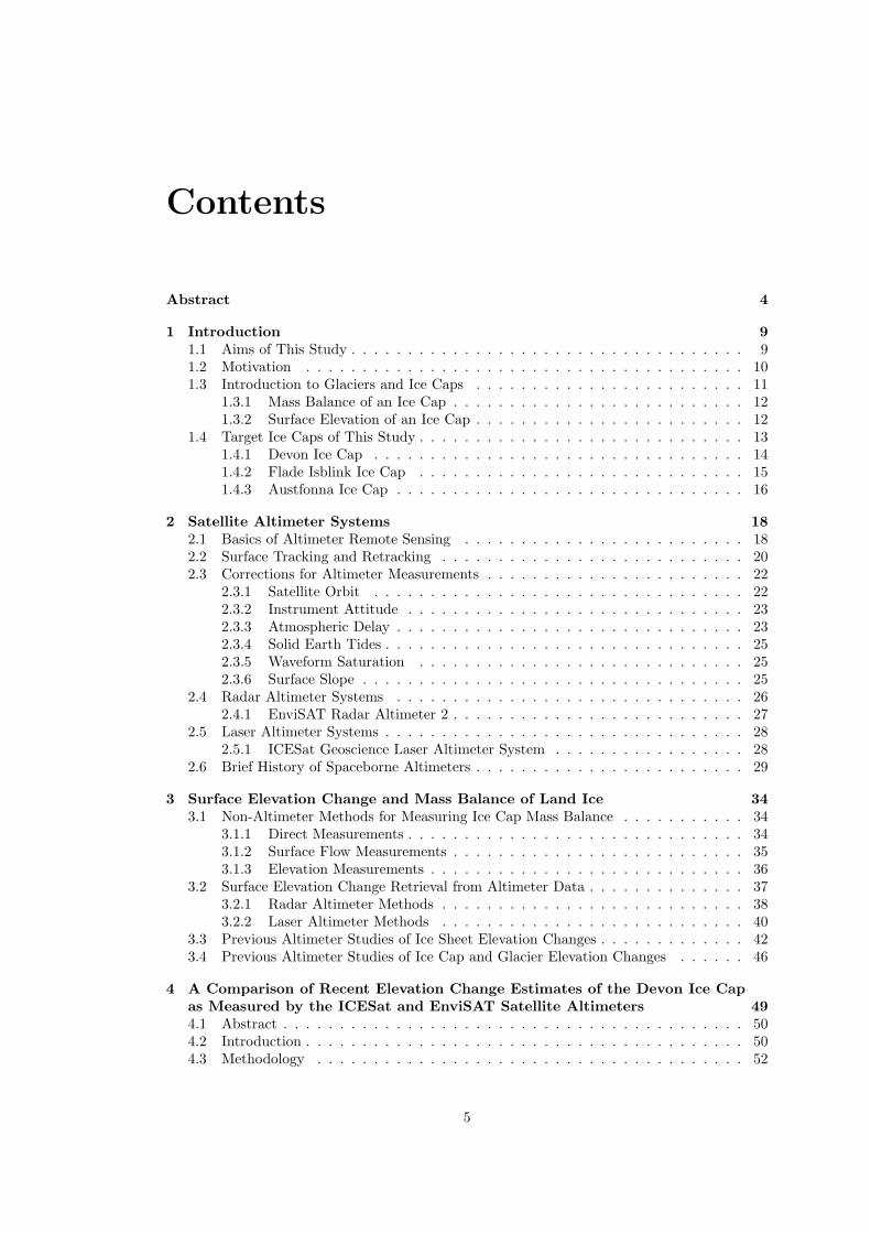
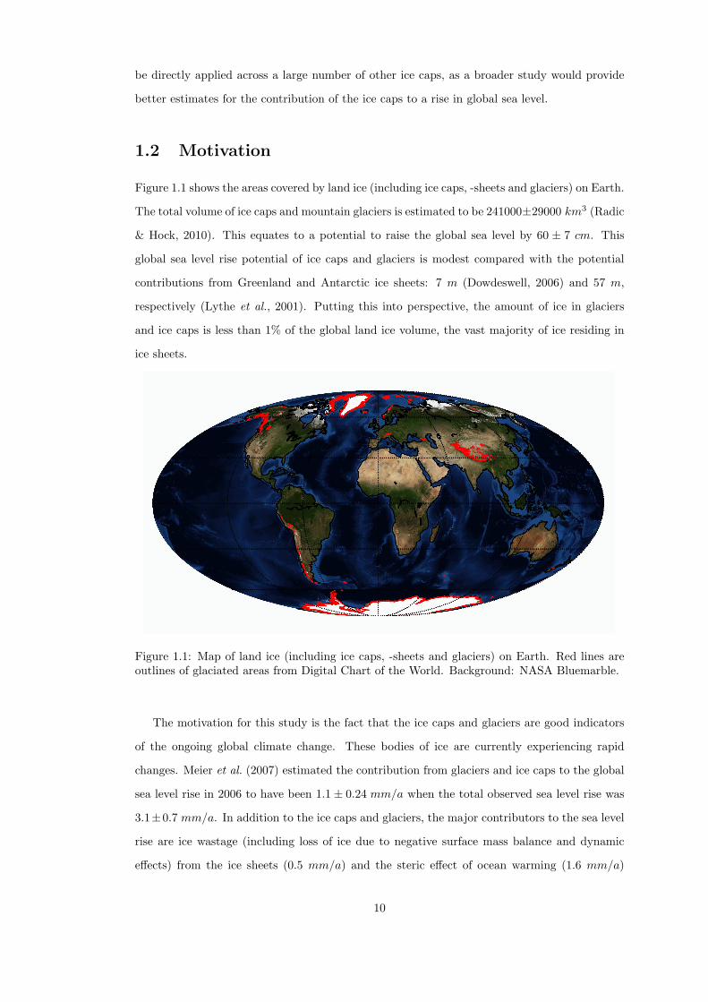
Figure 1.1 shows the areas covered by land ice (including ice caps, -sheets and glaciers) on Earth.
The total volume of ice caps and mountain glaciers is estimated to be 241000±29000 km3 (Radic
& Hock, 2010). This equates to a potential to raise the global sea level by 60 ± 7 cm. This
global sea level rise potential of ice caps and glaciers is modest compared with the potential
contributions from Greenland and Antarctic ice sheets: 7 m (Dowdeswell, 2006) and 57 m,
respectively (Lythe et al., 2001). Putting this into perspective, the amount of ice in glaciers
and ice caps is less than 1% of the global land ice volume, the vast majority of ice residing in
ice sheets.
Figure 1.1: Map of land ice (including ice caps, -sheets and glaciers) on Earth. Red lines areoutlines of glaciated areas from Digital Chart of the World. Background: NASA Bluemarble.
The motivation for this study is the fact that the ice caps and glaciers are good indicators
of the ongoing global climate change. These bodies of ice are currently experiencing rapid
changes. Meier et al. (2007) estimated the contribution from glaciers and ice caps to the global
sea level rise in 2006 to have been 1.1± 0.24 mm/a when the total observed sea level rise was
3.1±0.7 mm/a. In addition to the ice caps and glaciers, the major contributors to the sea level
rise are ice wastage (including loss of ice due to negative surface mass balance and dynamic
effects) from the ice sheets (0.5 mm/a) and the steric effect of ocean warming (1.6 mm/a)
10
(Meier et al., 2007). Future projections predict significant rates of volume loss from ice caps
and glaciers for the next century: according to a multi-model study by Radic & Hock (2010),
the sea level rise from glaciers and ice caps will amount to 12.4± 3.7 cm by 2100. This equates
to loss of one fifth of the total volume of ice in glaciers and ice caps today.
As mentioned earlier, the total sea level rise potential of glaciers and ice caps is an order
of magnitude smaller than that of ice sheets. The ice loss rate from the Greenland ice sheet
is increasing (Velicogna, 2009), and in fact may already have exceeded the ice loss rate from
glaciers and ice caps (Rignot et al., 2011). However, the sea level rise contribution of ice caps
and glaciers will remain significant during the next century. Also, because systems of different
sizes will possibly react differently to rising global temperatures, the study of all land ice bodies
is vital in the context of global warming.
This thesis investigates a satellite remote sensing method to assess the mass balance of
ice caps and glaciers. In contrast, past studies are heavily dependent on modelled data (e.g.
Radic & Hock (2011) and Meier et al. (2007)), relying on just a few direct observations for
calibration. Direct measurements of ice cap mass balance are point measurements by nature.
It is not feasible to cover a large ice cap with point measurements; ice caps can span thousands
of square kilometres of inhospitable terrain. Some past studies have utilised airborne data of
surface elevation. Alas, although spatially more extensive than point measurements, airborne
studies are usually limited to few transects over the target (e.g. Abdalati et al. (2004)). As
airborne campaigns are costly, they are also infrequent – at the very best one or two campaigns
per location per year. In contrast, satellite remote sensing provides near-global data with
reasonable revisit times. Even with the accuracy of satellite measurements poorer than that of
in-situ measurements, satellite studies are a valuable addition to the knowledge of the states of
and changes in the ice caps today.
1.3 Introduction to Glaciers and Ice Caps
A glacier is a perennial ice mass which moves over land. An ice cap is a dome-shaped body of ice
and snow that covers a mountain peak or a large area, and spreads out under its own weight. Ice
caps are in this sense a special case of glaciers. Ice often flows out from ice caps through outlet
glaciers, tongues of ice that extend from the main ice cap. Ice caps are often distinguished
from ice sheets by defining ice caps as being smaller than 50 000 km2 in size. Due to this
distinction, according to the American Meteorological Society, the Greenland and Antarctic
Ice Sheets should not be referred to as ice caps (Glickman, 2000). Ice caps are sometimes also
11
referred to as glacier caps. Historically they have also been called “plateu glaciers”, “island
ices” or “highland ices” (Sharp, 1956). The word “ice cap” has also been used to denote sea ice
in the Arctic Mediterranean. However, as the sea ice is largely seasonal this use of the word is
now considered improper (Glickman, 2000).
1.3.1 Mass Balance of an Ice Cap
The mass balance of an ice cap (the gain or loss of snow and ice due to accumulation and
ablation) is usually determined by the climate. An ice cap gains mass by percipitation of snow
at the ice cap surface. Ablation refers to processes that remove mass from the ice cap. These
include melting and evaporation, as well as different calving processes. As the ice cap flows
under its own weight, ice is transported out from the system by dynamic processes. Ice caps
can lose mass through breakaway of ice at their margins. Ice breaking into icebergs at water-
terminating glaciers is known as iceberg calving, whereas calving of land-terminating glaciers is
called dry calving. Advance of a land-terminating outlet glacier will not always affect the total
mass of an ice cap – it is possible that only the shape of the ice mass changes. The mass of
an ice cap can also change by basal melting, which can be significant locally (e.g. Dowdeswell
et al. (1999)), but was considered negligible at a global or large regional scale by the IPCC
(IPCC, 2007).
Many estimates of the global ice cap and glacier mass change are based on the surface mass
balance component only (for example Radic & Hock (2011)). Nevertheless, there are individual
glaciers where the dynamic component has been observed to dominate the mass balance over
surface effects (Arendt et al., 2006). Studies of glacier or ice cap mass changes due to changes in
ice dynamics are rare (Meier et al., 2007). Most importantly, the relative importance of surface
mass balance and ice dynamics can be only roughly estimated globally.
1.3.2 Surface Elevation of an Ice Cap
The surface elevation of an ice cap is a variable connected with, but different from, the mass
balance of an ice cap. A change in surface elevation can result from a change in mass, but it
can also be due to a change in the density or geometry of the ice cap. Ways of measuring ice
cap surface elevation are introduced along with ways of measuring mass balance in Section 3.1,
but the distinction between the two should be borne in mind. A negative elevation change does
not necessarily lead to a negative mass balance of the ice cap and consequential sea level rise.
The usefulness of surface elevation measurements lies in their being directly related to ice cap
volume. If the density of lost or gained material is known, mass change can be calculated from
12
volume change.
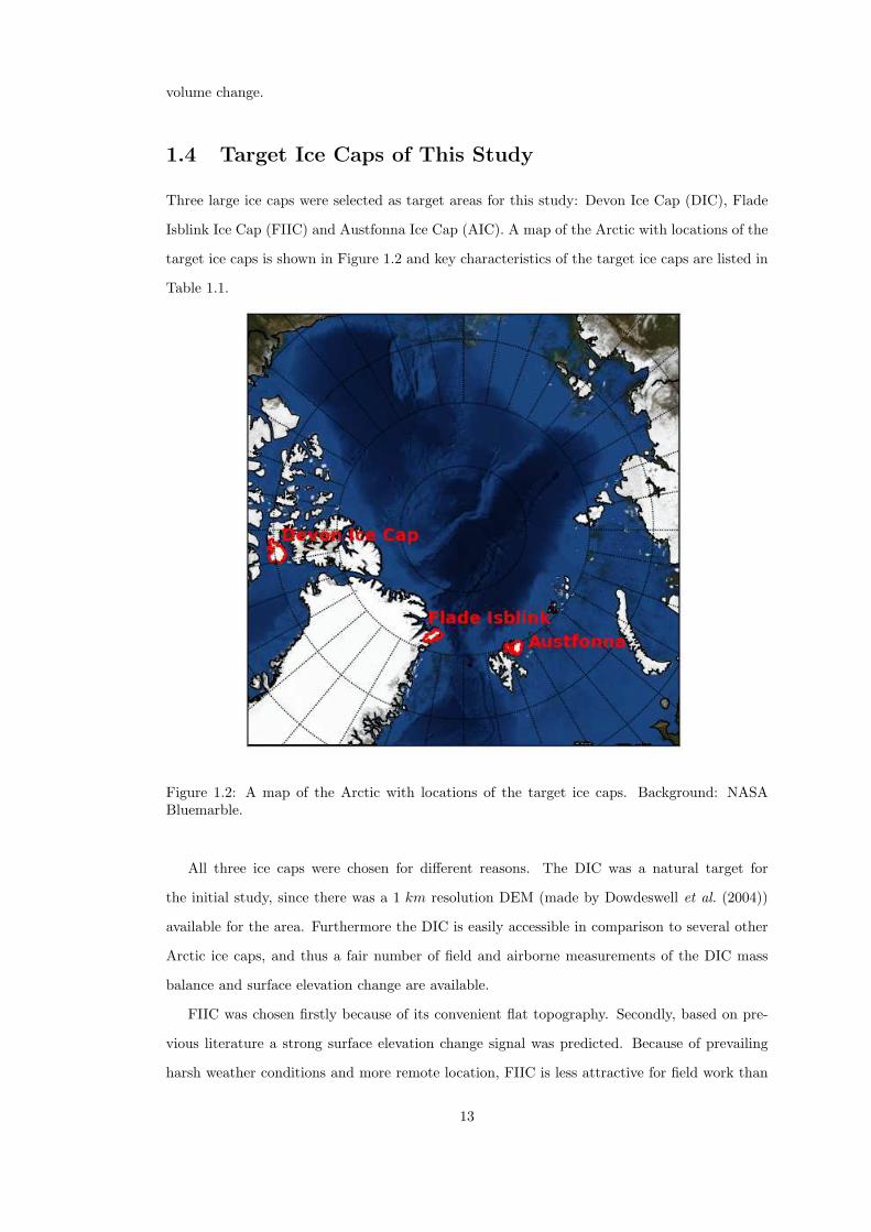
1.4 Target Ice Caps of This Study
Three large ice caps were selected as target areas for this study: Devon Ice Cap (DIC), Flade
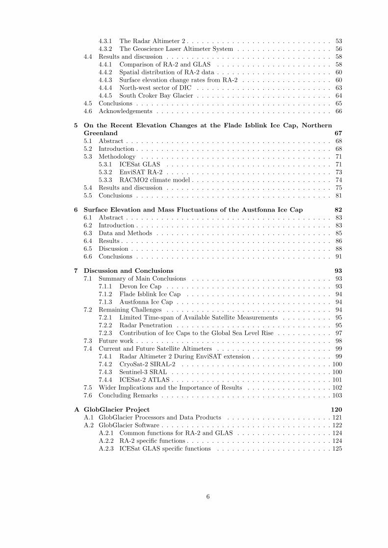
Isblink Ice Cap (FIIC) and Austfonna Ice Cap (AIC). A map of the Arctic with locations of the
target ice caps is shown in Figure 1.2 and key characteristics of the target ice caps are listed in
Table 1.1.
Figure 1.2: A map of the Arctic with locations of the target ice caps. Background: NASABluemarble.
All three ice caps were chosen for different reasons. The DIC was a natural target for
the initial study, since there was a 1 km resolution DEM (made by Dowdeswell et al. (2004))
available for the area. Furthermore the DIC is easily accessible in comparison to several other
Arctic ice caps, and thus a fair number of field and airborne measurements of the DIC mass
balance and surface elevation change are available.
FIIC was chosen firstly because of its convenient flat topography. Secondly, based on pre-
vious literature a strong surface elevation change signal was predicted. Because of prevailing
harsh weather conditions and more remote location, FIIC is less attractive for field work than
13
the DIC. Nevertheless, some field campaigns have been conducted in the FIIC (e.g. an echo
sounding campaign in 2006 (Laing, 2009)).
AIC was included to broaden the geographical extent of the study. Also, like in the case of
FIIC, a strong surface elevation signal was expected for AIC. There have been several studies
(in-situ by Pinglot et al. (2001), airborne by Bamber et al. (2004) and satellite altimeter by
Moholdt et al. (2010a)) of AIC mass balance. Both DIC and AIC are also target areas for the
Cryosat Validation and Calibration Experiment (CryoVEx).
The three three ice caps were the best candidates from their areas. The DIC because of
the data supporting our study available, the FIIC for its topography and the AIC for its large
size and multitude of past field campaigns. Other ice caps such as the ice caps on the Russian
Arctic islands of Novaya Zemliya, Severniya Zemliya and Franz Josef Land could had been
chosen as targets for closer study. They were not included in this study because of the lack of
previous elevation change studies and the limited access to the data collected during past field
campaigns.
Table 1.1: Key characteristics of the three target ice capsName Abbreviation Centre Coordinates Area [km2] Volume [km3]
Devon Ice Cap DIC 75 N 82 W 13700 3980Flade Isblink Ice Cap FIIC 81 N 16 W 8500 Not availableAustfonna Ice Cap AIC 79 N 24 E 8100 1900
1.4.1 Devon Ice Cap
DIC is a large ice cap on Devon Island in Nunavut, Arctic Canada, at 75oN and 82oW . Covering
an area of 13700 km2, the DIC is one of the largest ice caps on Earth. The DIC consists of
an 11700 km2 dome-shaped main ice cap and a 2000 km2 western arm that is stagnant and
dynamically separate (Dowdeswell et al., 2004). The main ice cap has a maximum elevation
of 1921 m and a maximum ice thickness of 880 m. The volume of the DIC is estimated to be
3980 km3 , which corresponds to about 10 mm of the global sea level rise potential.
There have been several studies on the mass balance of DIC. Accumulation rates have been
obtained from ice cores for example by Koerner (1977), Mair et al. (2005) and Colgan et al.
(2008). The Geological Survey of Canada has maintained a DIC surface mass balance stake
measurement network since 1961. Many studies have also utilized extrapolated weather data
and remote sensed ice velocity fields (e.g. Shepherd et al. (2007) and Burgess & Sharp (2008)).
Abdalati et al. (2004) used repeat airborne altimetry and estimated the surface elevation change
of DIC during 1995-2000. Although there is some disagreement about the absolute rate, all of
14
past studies agree that the DIC has been losing mass and contributing to global sea level rise
in recent decades.
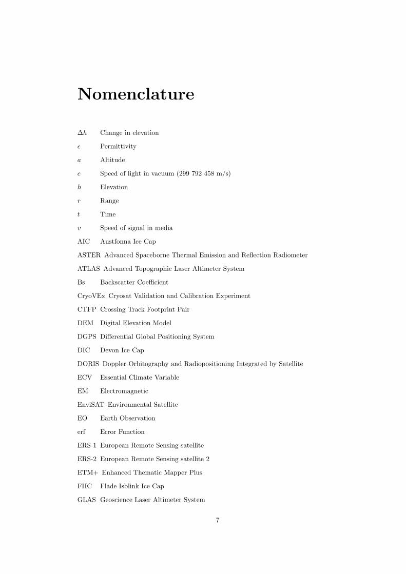
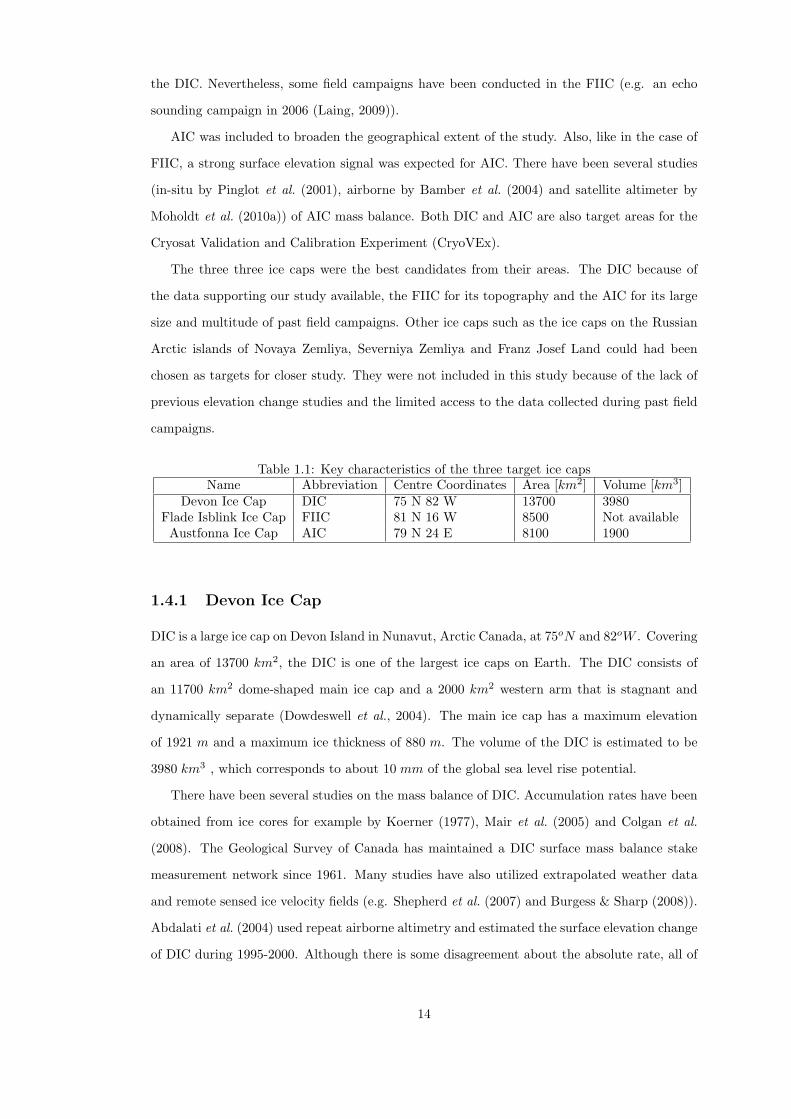
Map of the DIC by Burgess & Sharp (2008), showing locations and the extent of past
studies, is presented in Figure 1.3. The sparseness and limited coverage of measurements of
the DIC is striking: for example, the western arm has been excluded from past surface mass
balance studies. This underlines the need for efficient satellite altimeter studies of ice caps, a
task undertaken by this thesis.
Figure 1.3: Map of Devon Ice Cap from Colgan et al. (2008) showing locations and extentof past studies. Black lines are NASA altimetry flight lines (Abdalati et al., 2004). Contourspacing is 100 m with the 1200 m contour highlighted with a dashed line. Squares and circlesare shallow firn cores by Mair et al. (2005) and Colgan & Sharp (2008), respectively.
1.4.2 Flade Isblink Ice Cap
FIIC is a large ice cap in North East Greenland. Covering 8500 km2, it is the largest ice cap
in Greenland separate from the continental ice sheet (Kelly & Lowell, 2009). The aptly named
FIIC (“flade” stands for flat in Danish language) is characterized by low surface slopes in its
north-east part. The south-west part, which overlays the Princess Elisabeth Alps has steeper
slopes as well as some nunataks (exposed parts of underlying mountains). The maximum
elevation of the FIIC is approximately 960 m and ice thickness close to the central summit is
535 m. It is estimated that the FIIC may be a young ice cap of only a few thousand years
of age, much like the nearby Hans Tausen icecap (Lemark, 2009). The mass balance of the
15
FIIC is connected with the polynia (area of open water surrounded by sea ice) east of the ice
cap and the cold air available from the ice-covered ocean to the north and west of the ice cap
(Rasmussen, 2004).
There have been two previous studies describing surface elevation changes at the FIIC
(Krabill et al. (2000) and Pritchard et al. (2009)). Both of the studies have concentrated on the
Greenland Ice Sheet, but have also included elevation change estimates for the FIIC. Krabill
et al. (2000) conducted aircraft laser altimeter studies on Greenland for the years 1994 and
1999. Pritchard et al. (2009) included the FIIC in their study of Greenland ice sheet elevation
change using ICESat measurements during 2003-2008. Both studies agreed that the western
half of the FIIC was thickening at the rate of about 50 cm/a, whereas some areas near the
eastern margin were thinning.
FIIC was chosen as a target ice cap because of the large elevation change signal reported
by Krabill et al. (2000) and Pritchard et al. (2009). The flat topography suitable for satellite
altimetry also made the FIIC an interesting target area, and a high precision DEM by Palmer
et al. (2010) was available. In comparison to the two other target ice caps, the FIIC is relatively
little studied: for example there are no reliable estimates of its volume due to the lack of
extensive ice thickness measurements. The echo sounding campaign of 2006 covered only a
small fraction of the FIIC.
1.4.3 Austfonna Ice Cap
AIC is an ice cap in Nordaustlandet (“North-East -land”) in the Svalbard archipelago, Norway.
With a volume of 1900 km3 and an area of 8105 km2 (Dowdeswell, 1986), the AIC is the
fourth largest ice cap on Earth and the largest on Svalbard. AIC has been subject to keen
scientific study during the past decades. Extensive research on its mass balance using ice cores
was performed by Pinglot et al. (2001). According to this study, annual accumulation of snow
on AIC is 0.25% of its total mass. Such a high level of turnover renders studies of the ice
cap mass balance problematic, because there is considerable natural variability at seasonal and
inter-annual time scales.
According to an assessment (Hagen et al., 2003) of glaciological records the estimated mass of
AIC did not change significantly between 1963 and 1997. However, a series of more recent, short-
period surveys have reached markedly different conclusions. Repeat aircraft laser altimeter
measurements (Bamber et al., 2004) have shown that the central accumulation area thickened
significantly between 1996 and 2002. Bamber et al. (2004) suggested this to be due to a decline
of sea ice in the adjacent Barents Sea. Bevan et al. (2007) surveyed the ice cap mass budget
16

during the 1990s. Based on satellite-derived velocities, they detected an overall mass gain of
the ice cap. However, studies of mass balance of AIC by Dowdeswell et al. (2008) and Moholdt
et al. (2010a) found a negative mass change rate since the year 2000.
The main motivation for choosing AIC as one of the target areas was this large variation
of its past mass balance estimates. If all the past estimates of the AIC mass balance are valid,
the mass balance of AIC has recently changed sign. This makes AIC an interesting target for
any study.
17
Chapter 2
Satellite Altimeter Systems
This chapter presents altimeter systems that measure surface elevation. Basic altimeter op-
erating principles, surface tracking and retracking procedures, necessary corrections and the
difference between radar and laser altimeter systems are explained. Finally, a brief history of
satellite altimeters is included.
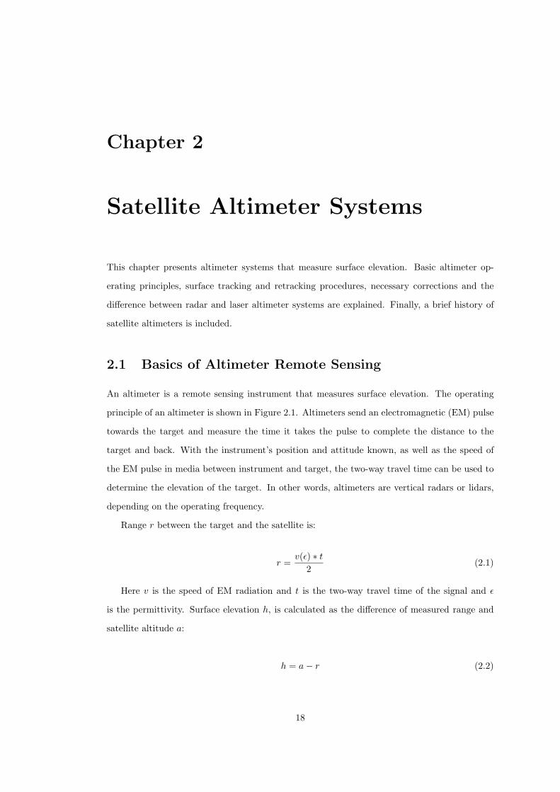
2.1 Basics of Altimeter Remote Sensing
An altimeter is a remote sensing instrument that measures surface elevation. The operating
principle of an altimeter is shown in Figure 2.1. Altimeters send an electromagnetic (EM) pulse
towards the target and measure the time it takes the pulse to complete the distance to the
target and back. With the instrument’s position and attitude known, as well as the speed of
the EM pulse in media between instrument and target, the two-way travel time can be used to
determine the elevation of the target. In other words, altimeters are vertical radars or lidars,
depending on the operating frequency.
Range r between the target and the satellite is:
r =v(ǫ) ∗ t
2(2.1)
Here v is the speed of EM radiation and t is the two-way travel time of the signal and ǫ
is the permittivity. Surface elevation h, is calculated as the difference of measured range and
satellite altitude a:
h = a− r (2.2)
18
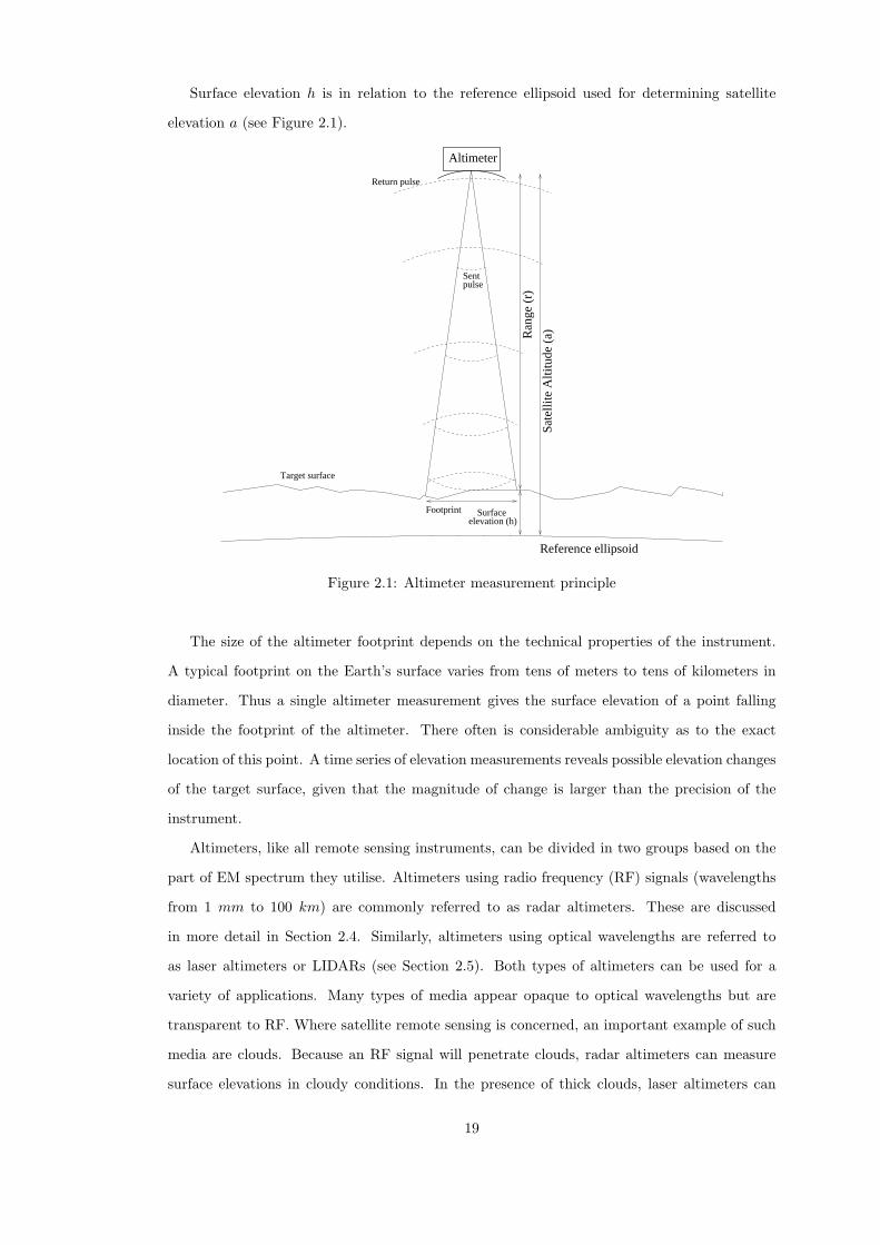
Surface elevation h is in relation to the reference ellipsoid used for determining satellite
elevation a (see Figure 2.1).
Return pulse
Sentpulse
Altimeter
Target surface
Footprint
Sat
ellit
e A
ltitu
de (
a)
Surface elevation (h)
Reference ellipsoid
Ran
ge (
r)
Figure 2.1: Altimeter measurement principle
The size of the altimeter footprint depends on the technical properties of the instrument.
A typical footprint on the Earth’s surface varies from tens of meters to tens of kilometers in
diameter. Thus a single altimeter measurement gives the surface elevation of a point falling
inside the footprint of the altimeter. There often is considerable ambiguity as to the exact
location of this point. A time series of elevation measurements reveals possible elevation changes
of the target surface, given that the magnitude of change is larger than the precision of the
instrument.
Altimeters, like all remote sensing instruments, can be divided in two groups based on the
part of EM spectrum they utilise. Altimeters using radio frequency (RF) signals (wavelengths
from 1 mm to 100 km) are commonly referred to as radar altimeters. These are discussed
in more detail in Section 2.4. Similarly, altimeters using optical wavelengths are referred to
as laser altimeters or LIDARs (see Section 2.5). Both types of altimeters can be used for a
variety of applications. Many types of media appear opaque to optical wavelengths but are
transparent to RF. Where satellite remote sensing is concerned, an important example of such
media are clouds. Because an RF signal will penetrate clouds, radar altimeters can measure
surface elevations in cloudy conditions. In the presence of thick clouds, laser altimeters can
19
only measure the height of the upper surface of clouds, and provide no information of Earth’s
surface.
2.2 Surface Tracking and Retracking
Initial coarse range processing is done on-board the satellite. An altimeter will have an on-board
waveform tracker. This is a system that will adjust the location of the range window, trying
to keep the waveform (power received by the altimeter as a function of time) centered on the
tracking point. In some applications it is enough to use the coarse delay information from the
tracking loop to estimate range, and thus elevation, of the target. However, when measuring
topographical targets such as land ice, the on-board tracker often fails to keep the waveform
centered. If the waveform moves outside the range window, the altimeter loses lock and is not
able to measure elevations until lock is regained. If the waveform is offset from the tracking
point and a high accuracy is called for, it is necessary to apply a range estimate refinement
procedure known as waveform retracking (Martin et al., 1983).
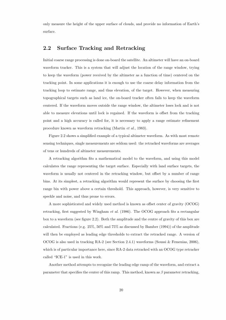
Figure 2.2 shows a simplified example of a typical altimeter waveform. As with most remote
sensing techniques, single measurements are seldom used: the retracked waveforms are averages
of tens or hundreds of altimeter measurements.
A retracking algorithm fits a mathematical model to the waveform, and using this model
calculates the range representing the target surface. Especially with land surface targets, the
waveform is usually not centered in the retracking window, but offset by a number of range
bins. At its simplest, a retracking algorithm would represent the surface by choosing the first
range bin with power above a certain threshold. This approach, however, is very sensitive to
speckle and noise, and thus prone to errors.
A more sophisticated and widely used method is known as offset center of gravity (OCOG)
retracking, first suggested by Wingham et al. (1986). The OCOG approach fits a rectangular
box to a waveform (see figure 2.2). Both the amplitude and the centre of gravity of this box are
calculated. Fractions (e.g. 25%, 50% and 75% as discussed by Bamber (1994)) of the amplitude
will then be employed as leading edge thresholds to extract the retracked range. A version of
OCOG is also used in tracking RA-2 (see Section 2.4.1) waveforms (Soussi & Femenias, 2006),
which is of particular importance here, since RA-2 data retracked with an OCOG type retracker
called “ICE-1” is used in this work.
Another method attempts to recognize the leading edge ramp of the waveform, and extract a
parameter that specifies the center of this ramp. This method, known as β parameter retracking,
20
was used by Martin et al. (1983) on Seasat waveforms from ice sheets. In addition to the OCOG
tracker mentioned above, RA-2 waveforms are also retracked using the ICE-2 retracker, which
is a β parameter retracker. The ICE-2 retracking of RA-2 waveforms is performed for all target
surfaces. Thus the choice of which retracker to use is left to the user. In the work at hand,
the ICE-1 retracker was chosen. This choice was made because the ICE-2 is optimized for
large flat ice sheets (Soussi & Femenias, 2006) and thus does not necessarily perform well with
topographic surfaces like the ice caps. However, the use of the ICE-2 is a configurable option
in the UCL altimeter processing software and thus ICE-2 could have been used.
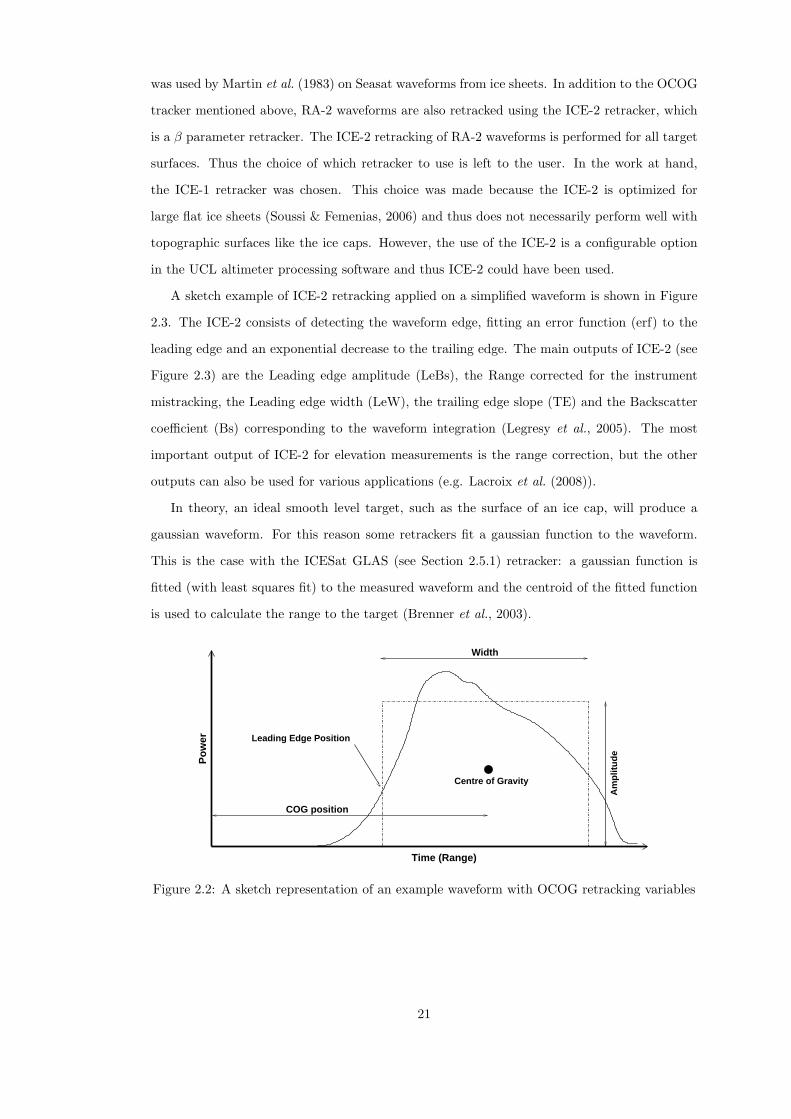
A sketch example of ICE-2 retracking applied on a simplified waveform is shown in Figure
2.3. The ICE-2 consists of detecting the waveform edge, fitting an error function (erf) to the
leading edge and an exponential decrease to the trailing edge. The main outputs of ICE-2 (see
Figure 2.3) are the Leading edge amplitude (LeBs), the Range corrected for the instrument
mistracking, the Leading edge width (LeW), the trailing edge slope (TE) and the Backscatter
coefficient (Bs) corresponding to the waveform integration (Legresy et al., 2005). The most
important output of ICE-2 for elevation measurements is the range correction, but the other
outputs can also be used for various applications (e.g. Lacroix et al. (2008)).
In theory, an ideal smooth level target, such as the surface of an ice cap, will produce a
gaussian waveform. For this reason some retrackers fit a gaussian function to the waveform.
This is the case with the ICESat GLAS (see Section 2.5.1) retracker: a gaussian function is
fitted (with least squares fit) to the measured waveform and the centroid of the fitted function
is used to calculate the range to the target (Brenner et al., 2003).
Time (Range)
Po
wer Leading Edge Position
Centre of Gravity
Width
Am
plit
ud
e
COG position
Figure 2.2: A sketch representation of an example waveform with OCOG retracking variables
21
2.3 Corrections for Altimeter Measurements
There are several variables that have effect on the range, and therefore surface elevation mea-
sured by a satellite altimeter. To achieve the best possible accuracy, the effect of these variables
must be compensated for.
2.3.1 Satellite Orbit
An altimeter is only able to measure the range r between the target and the altimeter itself (see
Figure 2.1. Any uncertainty in satellite elevation (also known as radial uncertainty) will carry
to altimeter elevation measurement making the radial uncertainty a major error source. In fact
the radial uncertainty has been the largest error source in recovering sea surface height or ice
sheet elevation from ERS altimeter measurements (Scharroo, 2002). Uncertainties in satellite
orbits result from uncertainties in Earth gravity models. Gravity anomalies of the Earth, as well
as the gravity of the sun and the moon, affect the orbit of any satellite. At the high altitudes
where EO satellites usually fly, air drag is low but at the same time highly variable and hard
to predict. Both gravity and air drag have an effect on the orbit.
Modern satellites measure their location with different positioning systems, such as Global
Positioning System (GPS) (used by ICESat (Zwally et al., 2002)) and Doppler Orbitography
and Radiopositioning Integrated by Satellite (DORIS) system (used by EnviSAT (Willis et al.,
2006)). In addition to GPS and DORIS, satellite orbit can be monitored by laser ranging from
the ground (e.g. Wingham et al. (2006)). Used in tandem, these systems allow the radial
component of satellite orbit to be determined with an accuracy of better than 5 cm which is
Time (Range)
Po
wer
Fitted model
Trailing edge slope (TE)
RangeBackscatter coefficient (Bs)
Leading egde width (LeW)
Lea
din
g e
gd
e am
plit
ud
e (L
eBs)
Figure 2.3: A sketch representation of an example waveform with ICE-2 retracking outputs andfitted function (red)
22
still one of the major components of the surface elevation measurement error budget.
In addition to the radial component, the cross-track and along-track offsets of the orbit may
also have an effect on the altimeter measurement. The actual orbit of a satellite is never the
exact nominal orbit but a cross-track offset is present. For EnviSAT, before the orbit change
in 2010, the target was to keep actual ground track within 1 km distance from the nominal
ground track. This was achieved 94% of the time as reported by Bargellini et al. (2006). If the
target geometry is not flat but there is a slope present, the altimeter measures the elevation of
“wrong” position on Earth’s surface due to the orbit uncertainty. With the DORIS system the
position of a satellite can be tracked with uncertainties of few tens of centimetres in along-track
and cross-track directions (Tavernier et al., 2003). The error due to this uncertainty is thus
negligible for the relatively flat surfaces relevant for this thesis.
2.3.2 Instrument Attitude
Even the most stable satellites oscillate for various reasons. For example, satellites carrying
adjustable solar panel arrays, like ICESat (see subsection 2.5.1), will oscillate due to solar array
motions. In case of ICESat, these oscillations produced tens of meters of cross-track motion of
the laser spot on the Earth’s surface (Schutz et al., 2005). A common way to measure satellite
attitude is to use star trackers. These instruments record the stars visible to the satellite,
and compare them to known star atlases to determine instrument attitude (Liebe, 1995). Star
tracker systems are complemented by gyroscope attitude control systems. For example, the
pointing uncertainty of GLAS onboard ICESat (which utilized both star trackers and gyroscope
attitude control) was less than 2 arcseconds, resulting into a geolocation uncertainty of less than
6 m (Schutz et al., 2005).
When measuring sloping surfaces, this instrument pointing error will transform into an
elevation error. This is due to instument measuring an elevation of the “wrong” location on
the Earth’s surface. Again using ICESat as an example, an uncertainty of one arcsecond in
pointing an instrument at 600 km altitude will result in 5 cm error in inferred elevation, if the
target surface slope is 1o (Schutz et al., 2005). This is an order of magnitude larger source
of uncertainty than what is introduced bu the cross-track and along-track orbit uncertainties
discussed in subsection 2.3.1.
2.3.3 Atmospheric Delay
In altimeter measurements it is essential to know the speed of signal in the media between the
target and the instrument. Whereas the speed of EM radiation in a vacuum, c (speed of light),
23
is a constant of exactly 299792458 m/s (SI Brochure, 2006) this is not the case for the speed
of light in the atmosphere v. The speed of EM radiation in a dielectric medium is a function
of the complex permittivity. Permittivity in turn is a function of the electric polarisability.
Thus v depends on both the frequency of the EM radiation and the density of charged particles
(electrons and ions) and dipoles in air. This is of particular importance to satellite altimeter
remote sensing: as the signal travels through the atmosphere, any ambiguity in v will carry
over to the elevation measurement.
The typical electric dipole in the atmosphere is the water molecule. Variable water quantities
in the troposphere can contribute errors of up to 45 cm to the radar altimeter measurement
(Keihm et al., 1995). Therefore a correction for the delay induced by water, or wet atmosphere
correction, has to be included in altimeter measurements. Water content in the atmosphere
needed for this correction can be estimated from passive microwave data (Keihm et al., 1995).
Ideally the wet atmosphere correction is derived from a radiometer flying with the same satellite
as the altimeter, like the ENVISAT-1 Microwave Radiometer (MWR) (Resti et al., 1999a) or
the TOPEX/Poseidon Microwave Radiometer (TMR) (Keihm et al., 1995).
Other gas molecules in the atmosphere also have an effect on the path delay of an altimeter
signal. This component is usually referred to as dry atmosphere correction. The magnitude of
the dry atmosphere correction is large – more than two metres. However, its temporal variation
is small, of the order of a few centimetres. Dry atmospheric correction can be estimated by
the Saastamoinen formula, the only variables needed being latitude and sea level pressure
(Saastamoinen, 1971). Pressure and other atmospheric variables for altimeter corrections are
often estimated from different atmosphere models (e.g. Resti et al. (1999a) and Wingham et al.
(2006)).
The free electrons in the ionosphere also will have an effect on the v of altimeter signal. As
the ionospheric delay is frequency-dependent, difference in the delays of two different frequency
pulses can be exploited in estimating the ionospheric range correction. This is one of the main
reasons why most modern satellite altimeters have two channels. Magnitude of the ionospheric
correction is from a few millimeters to 40 cm (Scharroo, 2002). If dual frequency measurements
are not available, the ionospheric correction can also be derived from the DORIS network (this
is the case for example with EnviSAT (Soussi & Femenias, 2006)) or from different models (e.g.
CryoSat, (Wingham et al., 2006)). The uncertainty of the ionospheric correction is a major
contributor to the uncertainty of the altimeter measurement. Scharroo (2002) estimated the
random error of the altimeter correction for the ERS-1 RA to have been 3 cm, which is of the
same magnitude as the radial uncertainty of the satellite orbit.
24
2.3.4 Solid Earth Tides
The solid earth exhibits tides due to the gravity pull of the moon and the sun. Furthermore, the
variations of Earth’s rotation axis, known as polar motion, cause deformation within the Earth
surface. Both of these deformations are well known (Cartwright & Edden (1973) and Wahr
(1985), respectively) and can be compensated for in altimeter measurements. Peak-to-peak
variations in polar motion are typically 10− 20mm over a year (Wahr, 1985). The magnitude
of solid earth tides and, in consequence, the correction needed to compensate for them is ±1m
(Scharroo, 2002).
2.3.5 Waveform Saturation
If the pulse returning to the altimeter has a higher energy than expected, the detector may
saturate. Saturation results in the peak of the waveform being cut off, which will cause signifi-
cant difficulties for retracking. For instance, the OCOG retracking will not work with saturated
waveforms. Waveform saturation is a known problem with ICESat GLAS (see subsection 2.5.1)
waveforms. For saturated waveforms (waveforms of which total energy is more than the “sat-
uration threshold energy”), the standard Gaussian fit processing of GLAS is biased toward
longer ranges, leading to low elevation estimates (Fricker et al., 2005). An empirical correction
is applied to all GLAS measurements where saturation is present. The GLAS saturation cor-
rection is significant and can be more than 20 cm for bright targets such as land ice covered
by fresh snow (Fricker et al., 2005). Similar bright target possibly resulting in the saturation
of radar altimeters is the flat sea surface. Saturated waveforms can be easily recognised and
either compensated for or discarded.
2.3.6 Surface Slope
The altimeter antenna is pointed at nadir, and the diameter of a beam-limited footprint can be
of the order of tens of kilometres. The first part of the reflected echo will come from that part of
the surface within the field of view that is closest to the satellite. Over flat surfaces, the closest
point on the surface is at the nadir point (the point directly under the satellite). Over sloping
or rough terrain this is not the case. Over sloping surface the retracked range is actually slant-
range to a point offset from nadir. If an external elevation model is available, measurement can
be corrected for slant range and re-located to the real point of first return (Bamber, 1994). For
example the RA-2 data for Antarctic and Greenland ice sheets (but not for other land areas) are
corrected using surface slope models (Soussi & Femenias, 2006). The sloping surface will also
25
decrease the total power received by the altimeter. Yet another separate difficulty connected
with measuring sloping surfaces is the uncertainty resulting from the instrument pointing error
on a slope (discussed in Section 2.3.2).
2.4 Radar Altimeter Systems
Radar altimeters are altimeters operating at radio and microwave frequencies. The vast majority
of satellite altimeters have been radar altimeters. The names of the frequency bands used in
this work are the ones described in IEEE Standard Letter Designations for Radar-Frequency
Bands (IEEE Frequency Bands, 2003). Frequency band names originate from military radars
in the second world war but the IEEE naming standard is in common usage in civilian radar
applications today.
A drawback of using traditional radar altimeters for ice cap observations is the instru-
ment’s relatively large ground footprint. The antenna field of view of RA-2 (introduced in
subsection 2.4.1), for example, is 1.3o in the Ku-band channel. This results in a circa 18 km
beam-limited ground footprint, although the instrument’s pulse-limited ground footprint is con-
siderably smaller (Soussi & Femenias, 2006). A simple way to limit the antenna field of view is
to increase the physical antenna size. In space instruments, upper antenna size is limited by the
mass budget and the size of the launcher payload bay. For example, the RA-2 antenna is 1.2 m
in diameter (Resti et al., 1999a). Using a higher frequency (shorter wavelength) would also lead
to a smaller footprint, but the highest practical frequency is limited by the attenuation in the
atmosphere, which increases rapidly with shortening wavelength. Furthermore, there are but
a few narrow frequency bands reserved for spaceborne altimetry above the Ku band (ITU-R
Radio Regulations, 2004)
In addition to the general error sources (see Section 2.3) there is an uncertainty source
specific to radar altimeter measurements over ice. This is the penetration of the radar signal
into the snow pack. If the snow is dry, a radar altimeter will measure an elevation below the
snow-air interface. In the case of wet snow, the instrument will measure the elevation of the
snow-air interface. A technique for estimating the amount of radar penetration is to consider
the received power. If the signal penetrates into the snow pack, part of the transmitted power
will be scattered back via volume scattering. More penetration will result in more volume
scattering, and thus more received power. When a thick dry snow pack is to be expected, as
in accumulation areas of the Antarctica, a power correction can be applied (Wingham et al.,
1998). If the power correction is not applied, the ambiguous penetration must be taken into
26
account by other means when interpreting any radar altimeter measurements. Also, if intending
to measure the snow surface, it is desirable to perform measurements at times when the snow
surface is wet. This approach is used in Chapters 5 and 6. Similarly, if measuring a target
under the snow, measurements are best limited to times when the snow layer is expected to be
dry. This is the reason why Laxon et al. (2003) used only winter measurements when measuring
the thickness of sea ice.
2.4.1 EnviSAT Radar Altimeter 2
The Radar Altimeter 2 (RA-2) is a nadir-looking pulse-limited radar altimeter, based on the
heritage of the ERS-1 RA. The RA-2 utilises a main nominal frequency of 13.575 GHz (Ku-
band) to measure the elevation of the ground surface. In addition to the Ku-band channel,
the RA-2 had a 3.2 GHz (S-band) channel for the compensation of the delay caused by the
ionospheric electron density (see Section 2.3.3). The S-band channel of RA-2 stopped working
on 17 January 2008 (ESA Online News Bulletin, 2008) and ionospheric corrections have since
been based on models. The primary target of the RA-2 is sea surface topography mapping, but
the altimeter has also been shown to be capable of mapping the elevation of polar ice sheets
(Brenner et al., 2007)) and the thickness of sea ice (Laxon et al., 2003).
The RA-2 flies on board ESA’s EnviSAT satellite, launched in March 2002. From the start
of the science mission until October 2010, EnviSAT operated in a 35-day repeat cycle orbit
with a high inclination of 98o. In late 2010 EnviSAT had already exceeded its original 5-year
nominal lifetime by almost 4 years. To save on-board hydrazine, EnviSAT was lowered to a
30-day repeat cycle orbit 17 km below the original orbit and the inclination corrections were
discontinued. This leads to the extension orbit drift in inclination. At the time of writing the
RA-2 is operating normally, and is expected to do so for up to another three years (ESA Online
News Bulletin, 2010a).
All previous satellite radar altimeters (see section 2.6) suffered data dropouts over areas
with difficult terrain. To tackle this problem, RA-2 has a different tracker philosophy (Roca
et al., 2009). The surface tracking system of the RA-2 is designed to be more robust than its
predecessors, comprising an onboard autonomous resolution selection logic (RSL) (Resti et al.,
1999a). Over rough terrain (coastal zones, land and ice), where data dropouts might occur,
RSL changes the instrument into a coarser resolution mode (Resti et al., 1999a). Legresy et al.
(2005) showed that the RSL extends the use of RA-2 to areas where past altimeters have failed.
Most importantly, work of Legresy et al. (2005) suggested that RA-2 is able to measure the
surface elevation of ice caps, in addition to ice sheets. The main objective of this thesis is to
27
establish the use of RA-2 for the mapping of ice cap surface elevation change.
2.5 Laser Altimeter Systems
Laser altimeters are altimeters operating at optical wavelengths. The most significant difference
(usually advantageous) of laser over radar altimeters is the small ground footprint. The footprint
of a satellite laser altimeter can be less than a hundred meters in diameter (Zwally et al., 2002),
in contrast to that of several kilometres for radar altimeters.
Forward scattering is a problem specifically for laser altimeters (for general sources of error,
see Section 2.3). In the presence of clouds or aerosols in the atmosphere, part of the signal can
be scattered. These scattered photons travel a longer path than photons that pass directly to
and from the target. Therefore the mean travel time of the return pulse is lengthened, and the
centroid of the pulse is shifted toward a later time (Duda et al., 2001). A method to avoid errors
due to forward scattering is to identify the presence of forward scattering from the waveform.
Forward scattering causes a long tail in the waveform (Fricker et al., 2005), and measurements
with such a tail can later be discarded.
Although airborne laser altimeters are widely used remote sensing instruments, there have
been only a few of them orbiting the Earth. This is due to laser altimeters being electrically
and mechanically more complicated than radar altimeters, making the space environment par-
ticularly harsh for them (Ott et al., 2006). However, satellite altimetry has been widely used in
measuring the surface topography of celestial bodies like the moon (Kaula et al., 1974), Mars
(Smith et al., 1998) and Mercury (Zuber et al., 2008), as well as the asteroids Eros (Cole et al.,
2001) and Itokawa (Mukai et al., 2007). In addition to general topography, the Mars Orbiter
Laser Altimeter (MOLA) has succesfully measured surface elevation changes due to the annual
cycle of snow on Mars (Smith et al., 2001) – a feat curiously close to the topic of this thesis,
albeit on a different planet.
2.5.1 ICESat Geoscience Laser Altimeter System
The Geoscience Laser Altimeter System (GLAS) was a beam-limited laser altimeter flying on
board NASA’s ICESat. The main objective of ICESat was to measure the elevation changes of
the Greenland and Antarctic ice sheets. ICESat also monitored cloud height and structure, sea
ice roughness, sea ice thickness and ocean surface elevation (Zwally et al., 2002). ICESat was
launched in January 2003 into a 600 km orbit with a high inclination of 94o, making it the first
satellite to carry a laser altimeter in a polar orbit around the Earth.
28
GLAS consisted of three separate lasers and was originally planned to operate continuously
for three to five years. Sadly, laser 1 failed after only 37 days of operation (Schutz et al., 2005).
Fearing a similar failure for lasers 2 and 3, measurements were limited to three operation periods
of approximately 30 days per year (Schutz et al., 2005). The ICESat was put into a 91-day
repeat orbit in October 2003. Each 30 day operation period corresponds to approximately 35%
of one repeat orbit cycle. From spring 2003 to fall 2009, ICESat completed 17 such operation
periods: one every spring and fall, as well as three additional summer periods (years 2004, 2005,
and 2006). ICESat ended its science mission in February 2010 with the failure of the last of its
three lasers. The spacecraft was successfully decommissioned from operations 14 August 2010
and debris from the ICESat spacecraft fell into the Barents Sea on 30 August 2010. GLAS
level-1B elevation data is available free of charge online from the National Snow and Ice Data
Center (NSIDC) (NSIDC GLAS data page, 2011).
Single shot error of a GLAS measurement was estimated pre-launch to be about 14 cm
(Zwally et al., 2002). Shuman et al. (2006) presented repeat track and crossover analysis of
GLAS/ICESat L2 Antarctic and Greenland Ice Sheet Altimetry Data (GLA12). They showed
these elevation data to have a relative accuracy of ±13.8 cm and a precision of just over 2 cm,
satisfying the pre-launch estimate. The role of GLAS data in this work is to validate the RA-2
derived elevation change estimates in Chapter 4. GLAS data is also used to assess the elevation
change of FIIC in Chapter 5.
2.6 Brief History of Spaceborne Altimeters
Both radar and laser altimeters have measured the topography of the Earth from space. The
first satellite altimeter in orbit was S-193, flying with the NASA’s Skylab space station launched
in 1973 (Figure 2.4). S-193 was a microwave Earth observing system that consisted of active
and passive instruments. One of the parts of S-193 was a simple radar altimeter operating at
13.9 GHz nominal frequency. S-193 had two major shortcomings: it could be operated for only
short periods at a time, and it needed an astronaut to operate the system. Its measurements
were thus limited to the reasonably short periods when Skylab was manned. The biggest feat
of the S-193 was to conduct nearly continuous radar altimeter measurements for one revolution
around the world (on 31 January 1974). S-193 was a groundbreaking experiment in many ways:
it demonstrated satellite altimeters to be technologically feasible, and it provided a dataset for
geodesic and oceanography research. (McGoogan et al., 1974)
The first satellite altimeter mapping land ice was the GEOS-3 altimeter. This was a Ku-
29
band radar altimeter designed to demonstrate the capability for directly measuring or inferring
geodetic, oceanographic and geophysical parameters (Stanley, 1979). The GEOS-3 satellite was
launched in April 1975 and ended its mission in December 1978. The main objective of GEOS-3
was the mapping of ocean geoids, and it was not anticipated that the altimeter would maintain
lock over topographical terrain. Happily GEOS-3 proved to provide valuable measurements
on land surfaces too: it was the first satellite altimeter to map the elevation profiles of the
Greenland Ice Sheet. Encouraged by the success of the GEOS-3 on Greenland, Brooks et al.
(1978) suggested that a satellite altimeter mission designed to measure land ice be placed in
polar orbit. This mission was realised 13 years later, in 1991, with the launch of the European
Remote Sensing satellite (ERS-1) carrying the Radar Altimeter.
There have been several satellites carrying radar altimeters since S-193 and GEOS-3. Seasat
(Figure 2.5), launched in 1978, was a short-lived satellite (105 days of glory). It carried a Ku-
band radar altimeter, largely built on the design of S-193 and GEOS-3, but with unprecedented
accuracy of better than 10 cm (MacArthur, 1976). Seasat altimeter, like its more modern
successors Geosat (McConathy & Kilgus, 1987), TOPEX (Fu et al., 1994), Jason-1 (Menard
et al., 2000) and Jason-2 (Bannoura et al., 2005), was designed to measure the world’s oceans.
For this reason it flew at a reasonably low inclination orbit of 66o, not reaching most of the
land ice on Earth. Satellites in low inclination orbits are generally of limited use for cryospheric
research. Seasat and Geosat both reached latitudes up to 72o, and thus did measure southern
parts of Greenland and part of the East Antarctic Ice Sheet. Combined dataset from Seasat
and Geosat satellite altimeters has been used to determine land ice elevation changes of these
areas (Zwally et al. (1989) and Davis et al. (2001)).
The ERS-1 was the European Space Agency’s first Earth-observing satellite. It was launched
on 12 July 1991 into a sun synchronous polar orbit at a height of 780 km. ERS-1 failed on
March 10, 2000, far exceeding its expected lifespan. The successor of ERS-1, ERS-2, was
launched on 21 April 1995. ERS-2 is still operational, despite many of the satellite’s hardware
systems (most notably the attitude control gyroscopes and the on-board tape recorder) having
failed. Both ERS satellites carried an array of Earth observation instruments, among them a
radar altimeter (RA). These are single frequency nadir-pointing radar altimeters operating in
the Ku-band. ERS-2, like its predecessor, is flying in a high inclination orbit of 98.2o. The high
inclination allowed RAs on board the ERS satellites to map surface elevation changes of Arctic
and Antarctic land ice. These studies are discussed in more detail in Section 3.2
The space shuttle has carried a laser altimeter on two missions: the Shuttle Laser Altimeter
(SLA) and Shuttle Laser Altimeter 2 (SLA-2) missions on board flights STS-72 in 1996 and
30
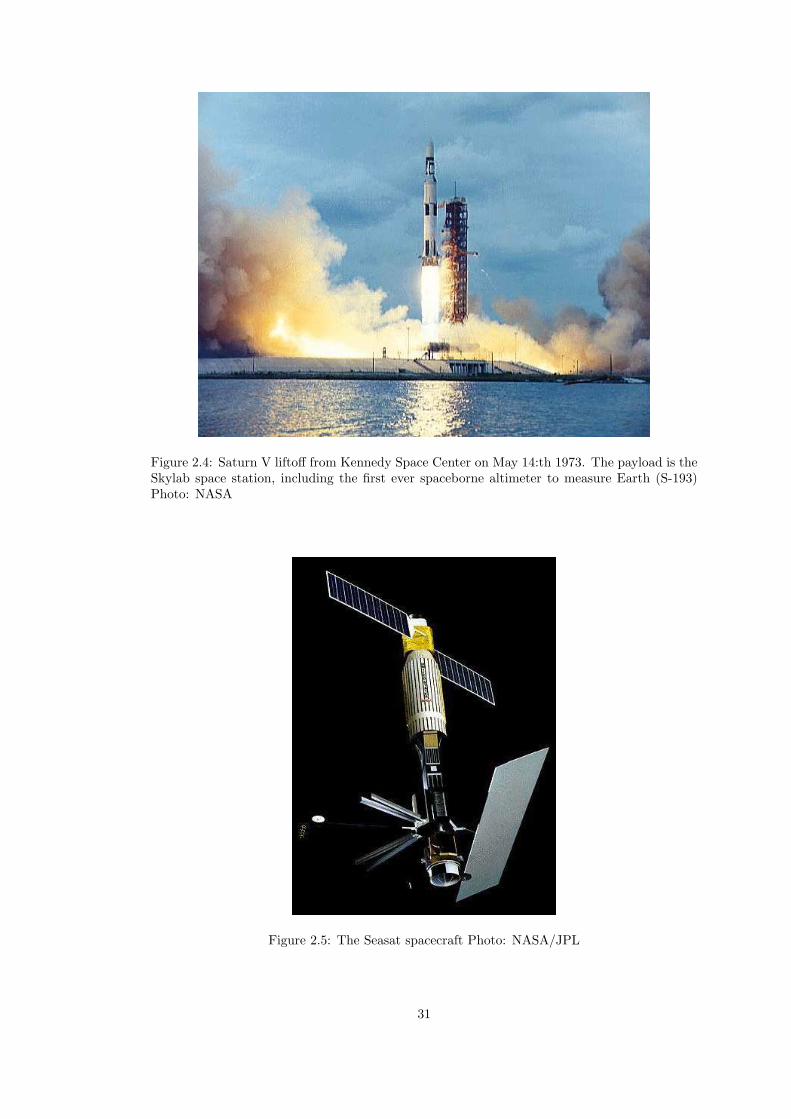
Figure 2.4: Saturn V liftoff from Kennedy Space Center on May 14:th 1973. The payload is theSkylab space station, including the first ever spaceborne altimeter to measure Earth (S-193)Photo: NASA
Figure 2.5: The Seasat spacecraft Photo: NASA/JPL
31

STS-85 in 1997, respectively (Garvin et al., 1998). Like all space shuttle missions, STS-72 and
STS-85 flew on a relatively low inclination orbit, and the SLA data has little value for mapping
land ice. However, the SLA experiments laid the groundwork for GLAS, which is one of the
two instruments utilised in this study. A summary of satellite altimeter missions is presented
in table 2.1.
32
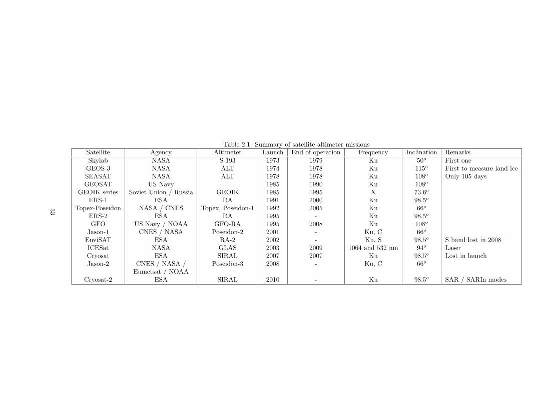
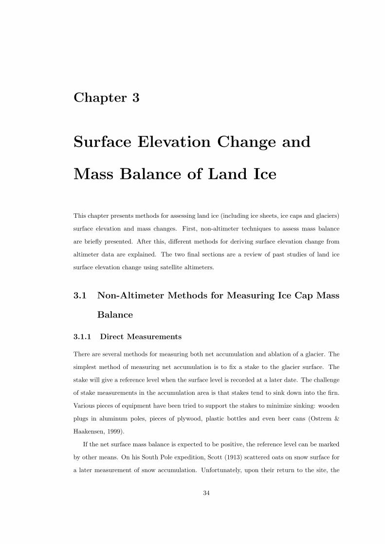
Table 2.1: Summary of satellite altimeter missionsSatellite Agency Altimeter Launch End of operation Frequency Inclination RemarksSkylab NASA S-193 1973 1979 Ku 50o First oneGEOS-3 NASA ALT 1974 1978 Ku 115o First to measure land iceSEASAT NASA ALT 1978 1978 Ku 108o Only 105 daysGEOSAT US Navy 1985 1990 Ku 108o
GEOIK series Soviet Union / Russia GEOIK 1985 1995 X 73.6o
ERS-1 ESA RA 1991 2000 Ku 98.5o
Topex-Poseidon NASA / CNES Topex, Poseidon-1 1992 2005 Ku 66o
ERS-2 ESA RA 1995 - Ku 98.5o
GFO US Navy / NOAA GFO-RA 1995 2008 Ku 108o
Jason-1 CNES / NASA Poseidon-2 2001 - Ku, C 66o
EnviSAT ESA RA-2 2002 - Ku, S 98.5o S band lost in 2008ICESat NASA GLAS 2003 2009 1064 and 532 nm 94o LaserCryosat ESA SIRAL 2007 2007 Ku 98.5o Lost in launchJason-2 CNES / NASA / Poseidon-3 2008 - Ku, C 66o
Eumetsat / NOAACryosat-2 ESA SIRAL 2010 - Ku 98.5o SAR / SARIn modes
33
Chapter 3
Surface Elevation Change and
Mass Balance of Land Ice
This chapter presents methods for assessing land ice (including ice sheets, ice caps and glaciers)
surface elevation and mass changes. First, non-altimeter techniques to assess mass balance
are briefly presented. After this, different methods for deriving surface elevation change from
altimeter data are explained. The two final sections are a review of past studies of land ice
surface elevation change using satellite altimeters.
3.1 Non-Altimeter Methods for Measuring Ice Cap Mass
Balance
3.1.1 Direct Measurements
There are several methods for measuring both net accumulation and ablation of a glacier. The
simplest method of measuring net accumulation is to fix a stake to the glacier surface. The
stake will give a reference level when the surface level is recorded at a later date. The challenge
of stake measurements in the accumulation area is that stakes tend to sink down into the firn.
Various pieces of equipment have been tried to support the stakes to minimize sinking: wooden
plugs in aluminum poles, pieces of plywood, plastic bottles and even beer cans (Ostrem &
Haakensen, 1999).
If the net surface mass balance is expected to be positive, the reference level can be marked
by other means. On his South Pole expedition, Scott (1913) scattered oats on snow surface for
a later measurement of snow accumulation. Unfortunately, upon their return to the site, the
34
expedition could not find the oats, thus providing a splendid example of the shortcomings of a
marker that will be covered completely by snow. Stakes fixed into the ice can also be used to
measure negative surface mass balance in ablation areas. A free-sliding horizontal arm is fixed
to two stationary stakes and placed on the ice surface. The vertical displacement due to ablation
is measured at a later time (Lewkowicz, 1985). Such ablation measurements will require two
visits to the field site for one measurement, but can be used to measure other timespans than full
years. Overall, in-situ measurements of surface mass balance are work-intensive and therefore
costly.
Net accumulation in the accumulation area can measured by identifying annual layers in a
firn sample. These layers can be characterized by changes in grain size or density. A dirt layer
representing summer ablation may also be present. Sometimes radioactive layers resulting from
human activities (e.g. nuclear tests or the Chernobyl accident) are present and can be utilised
(Pinglot et al., 2001). Reference layers resulting from known volcanic eruptions (Brandt et al.,
2005) as well as layers of high algae cell consentration (interpreted as annual summer layers)
have been used (Kohshima et al., 2007). Completely artificial markers, like the oats used by
Scott (1913), can also be used. The thickness of each layer multiplied by average density of the
snow corresponds to mean snow accumulation during the identified period. If annual layers are
resolved and identified, net accumulation estimates for individual years can be obtained from a
single firn core. If the net accumulation is negative (measurement is made in the ablation zone),
no new annual layers are generated and the current net mass balance cannot be measured by
coring.
Ground penetrating radar (GPR) provides yet another method to assess net accumulation.
A GPR is a low frequency (usually UHF or VHF band) radar with a signal that penetrates
into the snow pack. A GPR mounted on a sleigh can be used to obtain radar measurement
transects of the accumulation area. Internal reflection horizons visible in the radar echo can
be interpreted as previous summer surfaces (Kohler et al., 1997). GPR measurements are less
work-intensive than coring. However, the dielectric properties of the snow vary, which affects
the speed of the radar signal passing through snow pack. Therefore some coring is still needed
to calibrate the GPR. GPR is one of the standard techniques to measure snow accumulation
on glaciers today (Woodward & Burke, 2007).
3.1.2 Surface Flow Measurements
If ice velocity and thickess are known, the dynamic factor of the glacier mass balance can be
inferred. In practice, only the surface velocity of ice can be measured, and the internal velocity
35
has to be estimated from surface velocities. The surface flow of an ice cap can be remotely
measured using two fundamentally different techniques. The simpler of these is called feature
tracking. The key idea of feature tracking is to recognize features on ice cap surface in images
from two different datum. Observed difference in feature’s position can be used to determine
the glacier surface velocity (Lucchitta & Ferguson, 1986). Feature tracking of glacier flow has
been shown to be effective with optical data (Lucchitta & Ferguson, 1986) as well as Synthetic
Aperture Radar (SAR) amplitude and phase images (Strozzi et al., 2002). A more complicated
way to measure ice flow from space is by an interferometric synthetic aperture radar (InSAR)
(used for example by Palmer et al. (2010)), which is discussed in subsection 3.1.3. Ice velocity
can also be measured in situ by placing Global Positioning System (GPS) receivers on the ice.
3.1.3 Elevation Measurements
Before the satellite era, surface elevations had to be measured either terrestrially or with air-
borne studies. Traditional terrestrial methods include combined angle and distance measure-
ments, as well as optical levelling. These are very work-intensive by nature, and thus poorly
suited for large scale studies of ice caps spanning thousands of square kilometers.
Airborne stereophotogrammetry is a technique well suited to mapping elevations of large
areas (Kaab, 2005). It is possible to identify common features in two overlapping photographs
taken from different locations. Elevation of these features can be determined by triangulating
the lines of sight from the camera to the target. Stereophotogrammetry is not limited to airborne
studies; satellite instruments with forward- and backward-looking channels can be used as
well. The Advanced Spaceborne Thermal Emission and Reflection Radiometer (ASTER) is an
instrument currently flying with NASA’s Terra satellite. ASTER has forward- and backward-
looking channels, and thus ASTER images can be used to obtain digital elevation models
(DEMs) (Reuter et al., 2009). Unfortunately recognizing features on white flat ice caps in
ASTER imaginery is challenging. Combined with problems in cloud masking, this renders
ASTER DEM’s of poor quality over this study’s targets of interest.
Elevation models of ice caps and glaciers (as well as any other kind of terrain) can also be ac-
quired with interferometric synthetic aperture radar (InSAR). The basis of the InSAR techique
is a radar image pair of the same target from slightly different positions. Phase information of
the two images is interferred producing a phase difference map or an interferogram. The phase
difference is a function of target displacement and relative topography. If more than two radar
images are available, the topography is separable from the surface displacement field (Kwok &
Fahnestock, 1996). The relative elevations from InSAR can be tied to absolute elevations using
36
points of known absolute elevation (also known as ground control points or GCPs). In addition
to the DEM, InSAR also produces the velocity field of the target.
The Shuttle Radar Topography Mission (SRTM) created an extensive DEM of Earth surface
using an interferometric radar system flying onboard the space shuttle Endeavour in 2000.
SRTM utilised a radar with two antennas 60 m apart to acquire two radar images. Thus the
SRTM was a special case of InSAR radar, with two antennas acquiring images simultaneously.
Simultaneous acquisition eliminates the displacement field and thus only the topographic signal
is present in the interferogram. Endeavour flew at an orbit with an inclination of 57 degrees.
This allowed SRTM’s radar to cover the part of Earth’s surface lying between 60o north and 56o
south of latitude (Rabus et al., 2003). Most of the Earth’s land ice bodies lie at higher latitudes
than those covered by SRTM, and thus the SRTM DEM has only limited use in ice research.
However, (Sauber et al., 2005) employed SRTM to study the elevation change of Malaspina
glacier in southeastern Alaska (see Section 3.4).
Finally, land ice surface elevations can also be measured with the Global Positioning System
(GPS). This is an in-situ technique utilizing navigational satellite system. A GPS receiver is
mounted on a sleigh (or other moving platform) and dragged over the target. Accuracy of surface
elevation measurements of Arctic glaciers can be as good as 10 cm when using differential GPS
(DGPS) enhancement (Eiken et al., 1997), which utilises a reference GPS receiver at a well-
known location.
If DEM’s from different epochs in time are available, they can be used to assess the elevation
change and thus the mass balance of an ice cap. This technique is called DEM differencing. The
DEMs can be either in-situ measured or remote sensed. Point measurements from an altimeter
can also be compared to a DEM, resulting in point elevation change information (Kaab, 2005).
It is crucial to note that mass changes can be inferred from elevation change only when the
density of firn is known. Variance of firn density is recognized as one of the major causes of
uncertainty in measuring land ice mass balance with altimeters (Wingham, 2000).
3.2 Surface Elevation Change Retrieval from Altimeter
Data
Satellite altimeter data can be used in two different ways in assessing the elevation change
of the target. Elevation measured at an earlier date by other means can be subtracted from
satellite altimeter measured elevations, which will result in net elevation change between the two
measurements. The advantage of this approach is that it yields an estimate of mean elevation
37
change over periods longer than the relatively short lifespans of satellite missions. The downside
is that the accuracy of the elevation change estimate is dependent on the accuracy of both
measurements, and not only the precision of the satellite instrument.
To obtain the best results, both the DEM and the later elevation measurement should
be made using similar methods. For example, laser altimeter data should ideally only be
compared to DEMs based on laser altimeter measurements. Subtracting a DEM based on
radar measurements (such as SRTM) from elevation measured by GLAS will introduce an
uncertainty due to radar penetration into snow. In practice this has been done, because of the
scarcity of laser altimeter derived DEMs. For example Sauber et al. (2005) and Nuth et al.
(2010) have compared GLAS measurements to historic DEMs. Their results will be discussed
further in Section 3.4.
Another way of estimating the surface elevation change of a target from satellite altimetry is
to create a time series of elevation measurements from just one instrument. In addition to the
mean elevation change, this method allows one to reconstruct the surface elevation development
during the observation period. Precisely this approach is used in this thesis (Chapters 4, 5 and
6).
When surface elevation has been determined by waveform retracking (see Section 2.2) and
all the necessary corrections (see Section 2.3) have been applied, altimeter measurements can
be used for elevation change analysis in the two manners discussed above. Because of the
difference in footprint size, slightly different approaches have been used for laser and radar
altimeters. The most common elevation change retrieval methods are mentioned in Sections
3.2.1 and 3.2.2. Results from applying these methods to map the elevation change of land ice
bodies are presented in Sections 3.3 and 3.4.
3.2.1 Radar Altimeter Methods
Before my work on the DIC presented in Chapter 4, traditional radar altimeters had never
been used to map elevation changes of ice caps. However, a well-established methodology to
map elevation changes of ice sheets with radar altimeters does exist, and has been in use since
the late 1980’s (Zwally et al., 1989). All land ice elevation change studies are based on the
same methodology, referred to as the dh/dt-method by Zwally et al. (1989). The dual crossover
method (a special case of dh/dt-method, using only crossovers with two pairs of tracks), was first
used by Wingham et al. (1998) to define Antarctic elevation changes from ERS-1 measurements.
The foundation of the dual crossover method is to define the change in elevation, ∆h(x, t, tref ),
in orbital crossover points x between times t and tref . The change in elevation is measured in
38
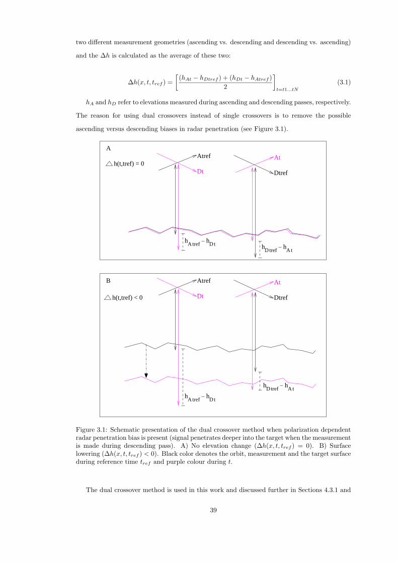
two different measurement geometries (ascending vs. descending and descending vs. ascending)
and the ∆h is calculated as the average of these two:
∆h(x, t, tref ) =
[
(hAt − hDtref ) + (hDt − hAtref )
2
]
t=t1...tN
(3.1)
hA and hD refer to elevations measured during ascending and descending passes, respectively.
The reason for using dual crossovers instead of single crossovers is to remove the possible
ascending versus descending biases in radar penetration (see Figure 3.1).
At
Dtref
Atref
Dt
At
Dtref
Atref
Dt
Atrefh
Dth
Dtrefh
Ath
Dtrefh
AthAtref
hDt
h
h(t,tref) < 0
h(t,tref) = 0
A
B
Figure 3.1: Schematic presentation of the dual crossover method when polarization dependentradar penetration bias is present (signal penetrates deeper into the target when the measurementis made during descending pass). A) No elevation change (∆h(x, t, tref ) = 0). B) Surfacelowering (∆h(x, t, tref ) < 0). Black color denotes the orbit, measurement and the target surfaceduring reference time tref and purple colour during t.
The dual crossover method is used in this work and discussed further in Sections 4.3.1 and
39
5.3.2. The development of radar altimeter methodology is presented alongside its results in
Section 3.3.
3.2.2 Laser Altimeter Methods
The only satellite laser altimeter so far, that has provided surface elevation data on significant
land ice targets, has been the GLAS. A method of deriving elevation change from residuals
at crossover points (similar to the methodology of Wingham et al. (1998)) was used by Smith
et al. (2005). The crossover point method is shown in Figure 3.2 A. However, all algorithms
building on crossover residuals will only provide information on elevation change at crossover
points. To map the elevation change between the crossover points, a different approach is
needed. Unfortunately, as the satellite track cannot be controlled to exactly coincide with the
nominal orbit, there is a spacing of up to hundreds of meters in repeat ICESat ground tracks.
If the target measured is not flat, and the consequent measurements are not from the exact
same location, an error due to local topography is introduced to the elevation change estimate.
Figure 3.2: Three methods to calculate elevation changes from GLAS data by Moholdt et al.(2010b). (A) linear interpolation of neighbour footprints to crossover pointss (dh = HA−HB),(B) cross-track DEM projection (HDREF = HD2 + dHDEM) and linear interpolation tocompare two repeat-tracks (dh = HDREF−HCREF ), and (C) fitting least-squares regressionplanes to repeat-track observations to estimate slopes and average dh/dt.
Slobbe et al. (2008) used elevations from overlapping GLAS footprint pairs to assess the
elevation change of the Greenland Ice Sheet. They used an external DEM to correct for bias
caused by the centre points of footprints not exactly coinciding. Overlapping footprints can
occur either in crossover locations (CTFP) or somewhere along track (RTFP) (see Figure 3.3).
Using overlapping footprints brings many more data points to the study than using crossovers
only.
Elevation change along-track can be estimated even when the footprints do not overlap.
Two techniques to achieve this are shown in Figure 3.2 B and C. The first one, referred to by
40
Moholdt et al. (2010b) as DEM-projected repeat-tracks, needs an external DEM which is used
to compensate for the effect of topography. This is similar to the approach of Slobbe et al.
(2008). GLAS method used in this study to assess the elevation change of FIIC is also a type
of DEM-projected repeat-track algorithm, and will be discussed in detail in Section 5.3.1.
If an external DEM is not available, or if the analysis is to be kept as independent from
external data as possible, the cross-track slope can be estimated by a surface fitted to elevations
measured during repeat-tracks (see Figure 3.2 C). In the study of the Greenland and Antarctic
ice sheets, Pritchard et al. (2009) fitted a triangular plane to three elevation observations, and
used the plane as the reference for measurements falling inside this triangle. Howat et al. (2008),
Moholdt et al. (2010a) and Moholdt et al. (2010b) used rectangular reference planes determined
by least squares fitting to segments of repeat-track GLAS data. Regardless of the shape of the
plane fitted, this approach eliminates the need for an external DEM. The disadvantage of the
plane fitting method is that the potential elevation change signal between the two repeat tracks
is present in the reference plane. However, Moholdt et al. (2010b) showed that both along-
track methods discussed here yield consistent results, and agree well with the elevation changes
calculated with crossover point method.
Figure 3.3: Schematic presentation by Slobbe et al. (2008) of two kinds of overlapping footprintpairs: Crossing Track Footprint Pairs (CTFPs) and Repeat Track Footprint Pairs (RTFPs).
41
3.3 Previous Altimeter Studies of Ice Sheet Elevation Changes
Altimeters such as GLAS, RA-2 and its predecessor RA have been used in mapping elevation
change of land ice bodies. Because all of the mentioned altimeters were designed and optimized
for large ice sheets, it is not suprising that most of the published work concentrates on Greenland
and Antarctic Ice Sheets.
Target of the first satellite altimeter elevation change study was the southern part of the
Greenland Ice Sheet. Zwally (1989) used Geosat and Seasat altimeter data and arrived at an
average thickening rate of 0.23± 0.04m/a. Due to low inclination of the satellites, measurements
were only available south of 72oN . Thickening was found at all elevations of the ice sheet, both
in ablation and accumulation zones. Measured elevation change rates by Zwally (1989) are
presented in Figure 3.4.
Figure 3.4: Average Greenland Ice Sheet surface elevation changes by elevation bands by Zwally(1989)
The RAs onboard ESA’s ERS-1 and ERS-2 satellites have been used to measure elevation
change of Antarctic ice sheet during years 1992-1996 (Wingham et al., 1998) (see Figure 3.5),
1995-2000 (Davis & Ferguson, 2004) and most recently 1992-2003 (Davis et al., 2005). All of
these studies have based their analysis on elevation change values measured at orbital crossover
points (earlier referred to as the dh/dt -method). All three studies agree on the general elevation
change pattern: the East Antarctic Ice Sheet has a small positive elevation trend, whereas the
42
West Antarctic Ice Sheet has a negative one.
Figure 3.5: The change in elevation from 1992 to 1996 (expressed in cm/a) of the Antarctic IceSheet by Wingham et al. (1998)
Similar studies, using data from the same altimeters and a data processing scheme based
on orbital crossover points, have also been undertaken for the Greenland Ice Sheet (Johan-
nessen et al., 2005) (see Figure 3.6). Another study combining RA data from the Greenland
and Antarctic ice sheets to estimate their contribution to global sea level rise was made by
Zwally et al. (2005). They combined ERS-1 and ERS-2 radar altimeter data from 1992-2002
to modelled firn densities (most importantly variations in density) and estimated the overall
contribution of ice sheets to be near zero at 0.05 ± 0.03 mm/a, the West Antarctic Ice Sheet
losing mass while the East Antarctic and Greenland Ice Sheets are gaining it (Zwally et al.,
2005).
ICESat GLAS measured elevations of the Greenland Ice Sheet have been compared with
earlier airborne laser altimeter elevation measurements by Thomas et al. (2006). They show
the same overall pattern of Greenland Ice Sheet elevation change as reported by Zwally et al.
(2005). Both studies agree on low altitude areas near ice sheet margins having negative elevation
trends, and high altitude areas having small positive elevation trends. The study by Thomas
et al. (2006) also shows that the GLAS data has good enough spatial resolution to measure small
areas of fast thinning, such as Jakobshavn Isbrae, Kangerlussuaq and Helheim glaciers and their
drainage areas. An even finer resolution study of southeast Greenland mass loss, using GLAS
43
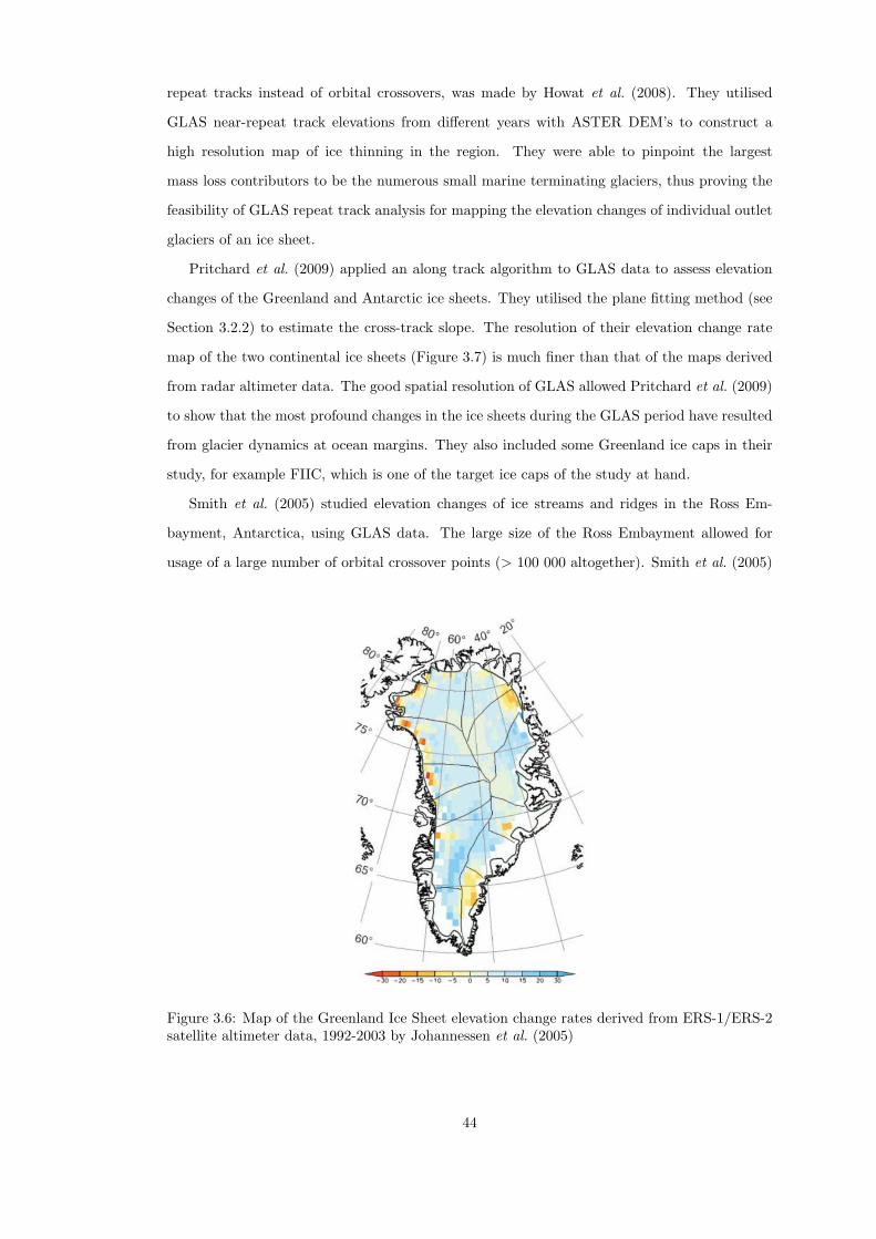
repeat tracks instead of orbital crossovers, was made by Howat et al. (2008). They utilised
GLAS near-repeat track elevations from different years with ASTER DEM’s to construct a
high resolution map of ice thinning in the region. They were able to pinpoint the largest
mass loss contributors to be the numerous small marine terminating glaciers, thus proving the
feasibility of GLAS repeat track analysis for mapping the elevation changes of individual outlet
glaciers of an ice sheet.
Pritchard et al. (2009) applied an along track algorithm to GLAS data to assess elevation
changes of the Greenland and Antarctic ice sheets. They utilised the plane fitting method (see
Section 3.2.2) to estimate the cross-track slope. The resolution of their elevation change rate
map of the two continental ice sheets (Figure 3.7) is much finer than that of the maps derived
from radar altimeter data. The good spatial resolution of GLAS allowed Pritchard et al. (2009)
to show that the most profound changes in the ice sheets during the GLAS period have resulted
from glacier dynamics at ocean margins. They also included some Greenland ice caps in their
study, for example FIIC, which is one of the target ice caps of the study at hand.
Smith et al. (2005) studied elevation changes of ice streams and ridges in the Ross Em-
bayment, Antarctica, using GLAS data. The large size of the Ross Embayment allowed for
usage of a large number of orbital crossover points (> 100 000 altogether). Smith et al. (2005)
Figure 3.6: Map of the Greenland Ice Sheet elevation change rates derived from ERS-1/ERS-2satellite altimeter data, 1992-2003 by Johannessen et al. (2005)
44
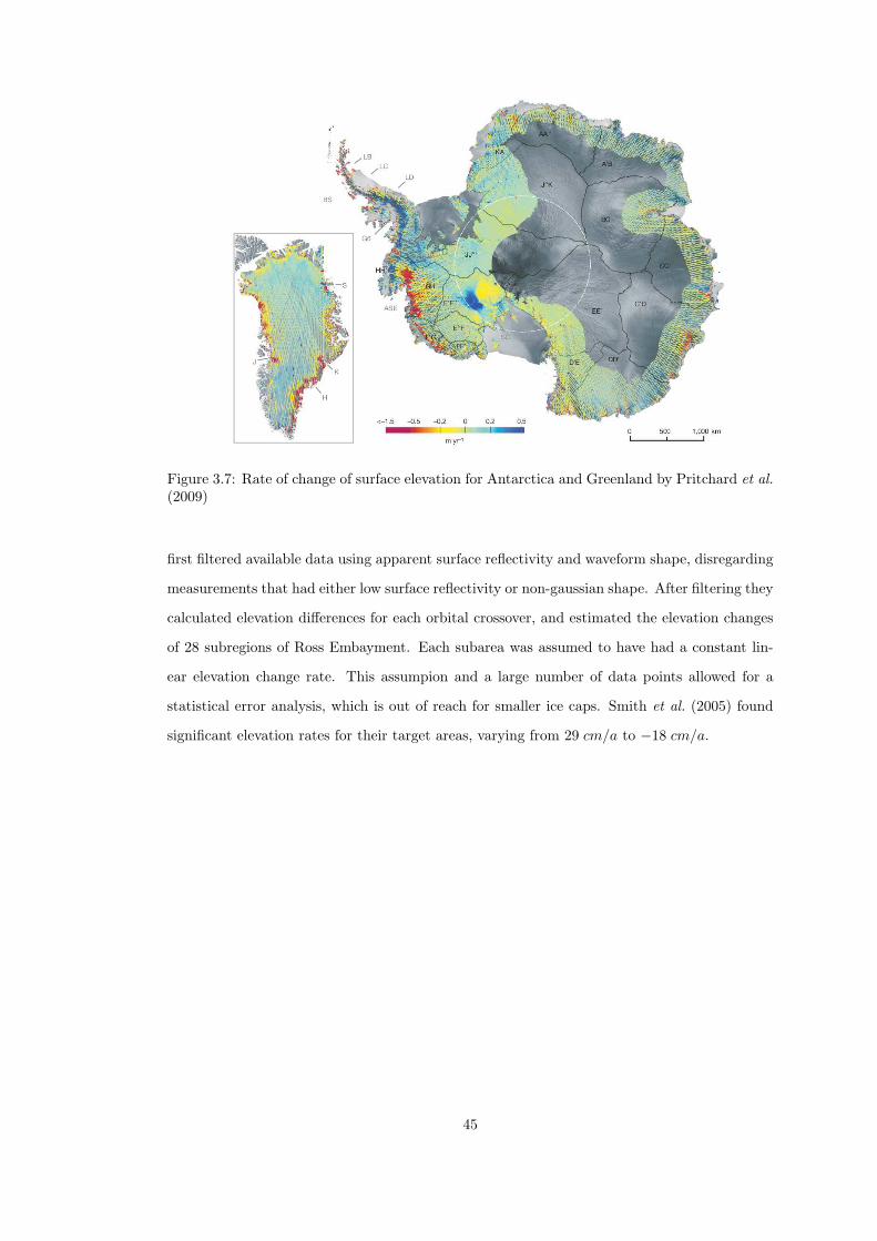
Figure 3.7: Rate of change of surface elevation for Antarctica and Greenland by Pritchard et al.(2009)
first filtered available data using apparent surface reflectivity and waveform shape, disregarding
measurements that had either low surface reflectivity or non-gaussian shape. After filtering they
calculated elevation differences for each orbital crossover, and estimated the elevation changes
of 28 subregions of Ross Embayment. Each subarea was assumed to have had a constant lin-
ear elevation change rate. This assumpion and a large number of data points allowed for a
statistical error analysis, which is out of reach for smaller ice caps. Smith et al. (2005) found
significant elevation rates for their target areas, varying from 29 cm/a to −18 cm/a.
45
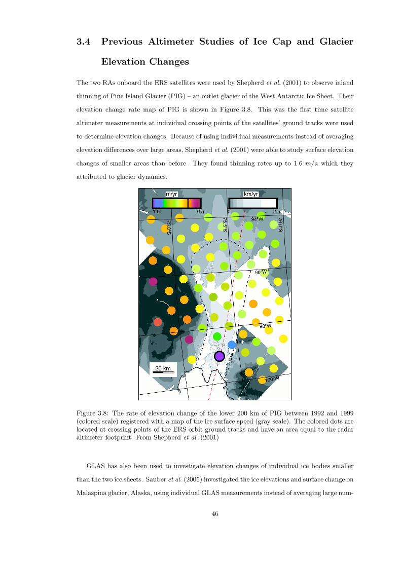
3.4 Previous Altimeter Studies of Ice Cap and Glacier
Elevation Changes
The two RAs onboard the ERS satellites were used by Shepherd et al. (2001) to observe inland
thinning of Pine Island Glacier (PIG) – an outlet glacier of the West Antarctic Ice Sheet. Their
elevation change rate map of PIG is shown in Figure 3.8. This was the first time satellite
altimeter measurements at individual crossing points of the satellites’ ground tracks were used
to determine elevation changes. Because of using individual measurements instead of averaging
elevation differences over large areas, Shepherd et al. (2001) were able to study surface elevation
changes of smaller areas than before. They found thinning rates up to 1.6 m/a which they
attributed to glacier dynamics.
Figure 3.8: The rate of elevation change of the lower 200 km of PIG between 1992 and 1999(colored scale) registered with a map of the ice surface speed (gray scale). The colored dots arelocated at crossing points of the ERS orbit ground tracks and have an area equal to the radaraltimeter footprint. From Shepherd et al. (2001)
GLAS has also been used to investigate elevation changes of individual ice bodies smaller
than the two ice sheets. Sauber et al. (2005) investigated the ice elevations and surface change on
Malaspina glacier, Alaska, using individual GLAS measurements instead of averaging large num-
46
ber of measurements. They found a thinning of five metres on the lower reaches of Malaspina
glacier, when comparing GLAS measurements from years 2003 and 2004 to the SRTM DEM
from February 2000. Work by Sauber et al. (2005) showed that GLAS data from glaciers can be
valuable, especially when there is an independent DEM available to support the analysis. The
challenge of near-repeat tracks not coinciding was tackled by differencing the ICESat along-
track measured elevations and the 2-dimensional SRTM DEM. The study shows that all of
the elevation differences of different tracks have similar long-wavelength features, and the two
tracks temporally close to each other also have similar short-wavelength features.
Nuth et al. (2010) compared GLAS elevation measurements to old topographic maps and
DEMs of the Svalbard archipelago. They were able to relate elevation changes to glacier dy-
namics, by showing that the glaciers that had surged were thickening in the ablation areas and
thinning in the accumulation areas.
The surface elevation and mass changes of Svalbard glaciers and ice caps were also investi-
gated by Moholdt et al. (2010b), using only GLAS data. Their elevation change rate map of land
ice in Svalbard is presented in Figure 3.9. Moholdt et al. (2010b) applied two different along-
track GLAS methods to assess the elevation changes. They concluded that the most glaciated
regions on Svalbard have experienced low-elevation thinning combined with high-elevation bal-
ance or thickening during the GLAS period 2003-2009. Moholdt et al. (2010b) also conpared
two different along track methods discussed in subsection 3.2.2. Finally, they estimated a total
mass loss rate of −4.3 ± 1.4 Gt/a for all the glaciers and ice caps on Svalbard. The study by
Moholdt et al. (2010b) was the first published study of the ice cap elevation changes using only
GLAS data. In the work at hand, the GLAS data is used for assessing the elevation changes of
FIIC (Chapter 5), as well as validating the RA-2 measurements on DIC (Chapter 4).
47
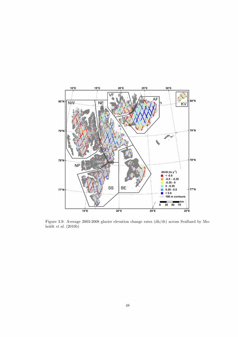
Figure 3.9: Average 2003-2008 glacier elevation change rates (dh/dt) across Svalbard by Mo-holdt et al. (2010b)
48
Chapter 4
A Comparison of Recent
Elevation Change Estimates of
the Devon Ice Cap as Measured
by the ICESat and EnviSAT
Satellite Altimeters
This chapter describes the comparison of measurements from two satellite altimeters on Devon Ice Cap
in Arctic Canada. This chapter has been published as “A Comparison of Recent Elevation Change
Estimates of the Devon Ice Cap as Measured by the ICESat and EnviSAT Satellite Altimeters”
Authors: Rinne, E.; Shepherd, A.; Muir, A.; Wingham, D.
Appears in: IEEE Transactions on Geoscience and Remote Sensing
Digital Object Identifier: 10.1109/TGRS.2010.2096472
Date of Publication: 06 January 2011
I processed the altimeter data from GLAS level 2 and RA-2 crossover elevation differences onwards.
The RA-2 crossover processing was done by Muir. I interpreted the results and wrote the manuscript.
Shepherd provided the original research idea, assisted with the interpretation of the data and writing
the manuscript.
49
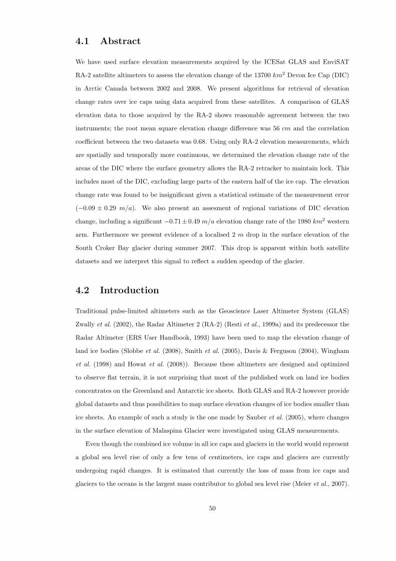
4.1 Abstract
We have used surface elevation measurements acquired by the ICESat GLAS and EnviSAT
RA-2 satellite altimeters to assess the elevation change of the 13700 km2 Devon Ice Cap (DIC)
in Arctic Canada between 2002 and 2008. We present algorithms for retrieval of elevation
change rates over ice caps using data acquired from these satellites. A comparison of GLAS
elevation data to those acquired by the RA-2 shows reasonable agreement between the two
instruments; the root mean square elevation change difference was 56 cm and the correlation
coefficient between the two datasets was 0.68. Using only RA-2 elevation measurements, which
are spatially and temporally more continuous, we determined the elevation change rate of the
areas of the DIC where the surface geometry allows the RA-2 retracker to maintain lock. This
includes most of the DIC, excluding large parts of the eastern half of the ice cap. The elevation
change rate was found to be insignificant given a statistical estimate of the measurement error
(−0.09 ± 0.29 m/a). We also present an assesment of regional variations of DIC elevation
change, including a significant −0.71±0.49 m/a elevation change rate of the 1980 km2 western
arm. Furthermore we present evidence of a localised 2 m drop in the surface elevation of the
South Croker Bay glacier during summer 2007. This drop is apparent within both satellite
datasets and we interpret this signal to reflect a sudden speedup of the glacier.
4.2 Introduction
Traditional pulse-limited altimeters such as the Geoscience Laser Altimeter System (GLAS)
Zwally et al. (2002), the Radar Altimeter 2 (RA-2) (Resti et al., 1999a) and its predecessor the
Radar Altimeter (ERS User Handbook, 1993) have been used to map the elevation change of
land ice bodies (Slobbe et al. (2008), Smith et al. (2005), Davis & Ferguson (2004), Wingham
et al. (1998) and Howat et al. (2008)). Because these altimeters are designed and optimized
to observe flat terrain, it is not surprising that most of the published work on land ice bodies
concentrates on the Greenland and Antarctic ice sheets. Both GLAS and RA-2 however provide
global datasets and thus possibilities to map surface elevation changes of ice bodies smaller than
ice sheets. An example of such a study is the one made by Sauber et al. (2005), where changes
in the surface elevation of Malaspina Glacier were investigated using GLAS measurements.
Even though the combined ice volume in all ice caps and glaciers in the world would represent
a global sea level rise of only a few tens of centimeters, ice caps and glaciers are currently
undergoing rapid changes. It is estimated that currently the loss of mass from ice caps and
glaciers to the oceans is the largest mass contributor to global sea level rise (Meier et al., 2007).
50
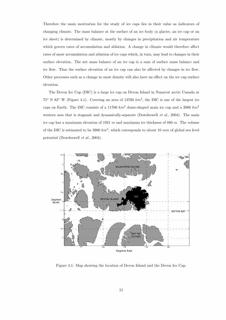
Therefore the main motivation for the study of ice caps lies in their value as indicators of
changing climate. The mass balance at the surface of an ice body (a glacier, an ice cap or an
ice sheet) is determined by climate, mostly by changes in precipitation and air temperature
which govern rates of accumulation and ablation. A change in climate would therefore affect
rates of snow accumulation and ablation of ice caps which, in turn, may lead to changes in their
surface elevation. The net mass balance of an ice cap is a sum of surface mass balance and
ice flow. Thus the surface elevation of an ice cap can also be affected by changes in ice flow.
Other processes such as a change in snow density will also have an effect on the ice cap surface
elevation.
The Devon Ice Cap (DIC) is a large ice cap on Devon Island in Nunavut arctic Canada at
75o N 82o W (Figure 4.1). Covering an area of 13700 km2, the DIC is one of the largest ice
caps on Earth. The DIC consists of a 11700 km2 dome-shaped main ice cap and a 2000 km2
western arm that is stagnant and dynamically-separate (Dowdeswell et al., 2004). The main
ice cap has a maximum elevation of 1921 m and maximum ice thickness of 880 m. The volume
of the DIC is estimated to be 3980 km3, which corresponds to about 10 mm of global sea level
potential (Dowdeswell et al., 2004).
Figure 4.1: Map showing the location of Devon Island and the Devon Ice Cap.
51
Previous literature exists on net mass balance, surface mass balance and surface elevation
change of the DIC. Estimates of mass and volume changes of the DIC have mainly relied on
snapshots of satellite or airborne data acquired with long (annual to decadal) time intervals.
Burgess & Sharp (2008), for example, estimated the volume loss of the DIC to have been
76.8 ± 7 km3 water equivalent between the years 1960 and 1999. They used a wide range
of data, including in-situ observations of surface mass balance, snow accumulation and ice
velocity, satellite measurements of ice velocity as well as modelled estimates of iceberg calving
and melting in the ablation zone. This volume change corresponds to an average deflation rate of
1.9±0.2 km3/a w.e. Other estimates of the DIC volume loss are smaller: for example, Shepherd
et al. (2007) estimated that the DIC was losing mass at the rate of 1.08 ± 0.67 km3/a w.e.
based on InSAR measured ice velocities from year 1996, interpolated snow accumulation rates
(measured at weather stations around DIC) and modelled runoff. Mair et al. (2005) compared
net accumulation rates determined from shallow cores to modelled runoff and estimated the
DIC to have lost on average 1.6± 0.7 km3/a w.e. between 1963-2000. Although there is some
disagreement about the absolute rate, all of these studies agree that the DIC has been a net
contributor to global sea level rise over recent decades. The only previous study on the surface
elevation change of the DIC was done by Abdalati et al. (2004). Using repeat airborne altimetry,
they estimated the surface elevation change to have been near-zero or slightly negative during
1995-2000. Here, we use repeat elevation measurements acquired by the GLAS and RA-2
satellite altimeters to estimate surface elevation change between 2002 and 2008. This is the
first time the surface elevation change over most of the DIC has been resolved at monthly time
intervals.
4.3 Methodology
In this study we utilise direct surface elevation measurements from two satellite altimeter mis-
sions (ICESat GLAS and EnviSAT RA-2) to estimate surface elevation changes of the DIC.
Our method differs from previous studies of the DIC by Mair et al. (2005), Shepherd et al.
(2007), Burgess & Sharp (2008) and Colgan et al. (2008), based on estimates of ice velocity and
surface mass balance. These estimates have been sparse in both space and time and have relied
upon regionally extrapolated measurements of accumulation and runoff estimates from different
models. Mair et al. (2005), Shepherd et al. (2007), Burgess & Sharp (2008) and Colgan et al.
(2008) have also estimated the mass balance of the DIC, a quantity related to but different
than surface elevation change. Instead of combining several sources of information, we rely
52
on direct measurements of surface elevation. Although NASA airborne altimeter campaigns in
1995 and 2000 at Canadian Arctic ice caps allowed elevation changes to be determined at the
DIC (Abdalati et al., 2004), the data were limited to just two flight lines and to two epochs in
time. It is difficult to assess the extent to which they are representative of changes across the
remainder of the DIC. Our method employs data that are distributed more widely in space and
time, and allow us to produce the first time-series of surface elevation with both good temporal
resolution and a reasonable spatial spread over the ice cap.
The current extent of the DIC has been derived within the framework of the European
Space Agency (ESA) GlobGlacier project (Paul et al., 2008) using Landsat ETM+ satellite
data acquired in 2000 and semi-automated mapping techniques (Paul & Kaab, 2005). The
same ETM+ images have been previously used by Burgess & Sharp (2004) to assess the extent
of the DIC using different delineation techniques. Only the elevation measurements falling
inside the GlobGlacier DIC outline are used in this study.
We used separate approaches in constructing elevation change estimates from RA-2 and
GLAS data. For both datasets, we endeavoured to minimize the use of external data, such as
digital elevation models (DEM). For the RA-2 data, we have chosen a dual crossover method
similar to that employed in previous studies utilising the RA-2 predecessor, the European Re-
mote sensing Satellite (ERS) Radar Altimeter (Wingham et al. (1998) and Johannessen et al.
(2005)). The method works well given populous time-series of data and our processing chain is
independent of external datasets. Although the GLAS provides surface elevation measurements
similar to those of the RA-2, the data are temporally sparse (typically 0-3 GLAS elevation mea-
surements per crossover location per year depending on clouds, in contrast to 11 per crossover
location per year from the RA-2) and so we adopted a different approach in processing GLAS
data. Instead of dual crossovers we use single-cycle crossovers from each period of GLAS oper-
ations. A consequence of this approach is that an external DEM was required to compensate
for the effects of surface slope on the GLAS elevation measurements.
4.3.1 The Radar Altimeter 2
The RA-2 is a nadir-looking, pulse-limited radar altimeter, based on the heritage of the ERS-1
RA. RA-2 utilises a main nominal frequency of 13.575 GHz (Ku Band) to measure the elevation
of the ground surface. In addition to the Ku-band channel, RA-2 has a 3.2 GHz (S-band) channel
for compensation of the delay due to ionospheric electron density. Sea surface topography
mapping is the primary target of RA-2, but the instrument is also able to map the elevation
of sea ice and polar ice sheets (Resti et al., 1999a). RA-2 flies onboard the ESA EnviSAT
53
-satellite, launched in March 2002. EnviSAT operates in a 35-day repeat cycle orbit, and
provides observations of most of the Earth surface between 81.5o N and 81.5o S. Whereas
previous radar altimeters have suffered data dropouts over areas with difficult terrain, the
surface tracking system of RA-2 is designed to be more robust. The RA-2 provides valuable
data for applications involving ice edges, land, lakes, wetlands and coastal zones (Benveniste
et al., 2008). The autonomous resolution selection of RA-2 has been shown to work on land and
ice surfaces like the DIC, circumstances where its predecessor (RA) failed (Roca et al., 2009).
The RA-2 has delivered a continuous dataset of global elevation measurements since 2002.
A major advantage of radar altimetry (as opposed to laser altimetry) is that the data are
not dependent on clear sky conditions. Microwave instruments can measure through clouds,
unlike optical instruments such as the GLAS. A drawback of the RA-2 for application to ice
caps is the instrument’s relatively large ground footprint; the antenna bandwidth (1.3o in
the Ku-band channel) results in a circa 18 km beam-limited ground footprint (although the
instrument’s pulse-limited ground footprint is considerably smaller (Soussi & Femenias, 2006)).
Another potential difficulty is caused by ambiguous penetration of radar signals into the snow
surface; for example, if the snow is dry, the RA-2 will measure an elevation below the the snow-
air interface, whereas if the snow is wet, the RA-2 will measure an elevation of the snow-air
interface. (Legresy et al., 2005)
The foundation of our processing chain is to define the change in elevation, ∆h(x, t1, t2), in
orbital crossover points x between times t1 and t2. An orbital crossover point is a point where
ascending and descending satellite ground tracks meet. We compare elevation measurements
from pairs of orbital cycles, acquired at times t1 and t2. Instead of combining ascending
and descending tracks from a single orbital cycle, we pair ascending track from cycle 1 with
descending track from cycle 2, and vice versa. In this manner we get two pairs of elevations:
ascending track elevation hAt1 (measured during orbit cycle 1 at time t = t1) and descending
track elevation hDt2 (measured during orbit cycle 2 at time t = t2), as well hAt2 (ascending
track, orbit cycle 2) and hDt1 (descending track, orbit cycle 1). The change in elevation between
two orbital cycles at each point is defined:
∆h(x, t1, t2) =(hAt1 − hDt2)− (hAt2 − hDt1)
2(4.1)
We assume the elevation change during one orbit cycle (maximum of 35 days) to be neglible.
Elevations at orbital crossover points were interpolated from the two nearest measured eleva-
tions h to the crossover point. To see how the surface elevation changes over time, we choose
one of the orbital cycles as a reference cycle. Pairing all other orbital cycles with the reference
54
cycle we obtain a time series of values of surface elevation ∆h(x, t, tref ) relative to the the
surface elevation measured during reference orbital cycle:
∆h(x, t, tref ) =
[
(hAt − hDtref ) + (hAtref − hDt)
2
]
t=t1...tN
(4.2)
To reduce noise, values of ∆h(x, t, tref ) are binned into 10 km cells and then averaged. To
study average elevation changes of larger areas the size of the data bin can be varied. The
resulting time series is affected by the choice of the reference cycle: each single cycle may have
missing data or other anomalies. Instead of choosing only one reference cycle we have created
multiple time series of ∆h using different suitable tref . These time series were further processed
by subtracting an average of ∆h over time from values of ∆h, producing the variation relative
to mean elevation at each point:
∆h(x, t, tref ) = ∆h(x, t, tref )−
∑ni=1
∆h(x, ti, tref ))
n(4.3)
Finally, a set of such time series was combined for trend analysis.
We discarded ∆h values deviating by more than 3 standard deviations of ∆h over time in
each bin. After this 3-sigma clipping, a first degree polynomial P∆h was fitted to the time
series of ∆h in each bin; the slope of this function represents the elevation trend dh/dt. Overall
trend is acquired from the slope of a first degree polynomial, even if the elevation change of an
ice cap is not always linear. We could have used the difference of the first and last elevation
measurement (being analoguous to two altimeter campaigns at different times) but our chosen
method is less sensitive to error in single measurement or anomalous circumstances during
one of the measurements times. In addition to overall trend, the resulting time series yields
information on surface elevation development through the study period. We discuss this further
in subsections 4.4.4 and 4.4.5.
The most relevant error sources contributing to the radar altimeter measurement are radar
speckle, noise introduced by sub-footprint surface topography and penetration of the radar
signal into the snow-pack. All of these error sources are functions of time and place and, in
general, are poorly known - especially so on an ice surface with non-zero slopes. In the absence
of formal estimates of error for the RA-2 over ice caps,we have derived an error estimate from
residuals between measured ∆h and a linear polynomial. Our error estimate edh/dt for elevation
trend dh/dt(x) over the observation period is defined as:
edh/dt =
∑ni=1
|∆h(ti)− P∆h(ti)|
n ∗ (max(t)−min(t))(4.4)
55
Forming an error estimate based on variations of the elevation measurements is supported
by an earlier study of Radar Altimeter data, which compared the measured elevation change
error covariance and the estimated covariance of different error contributions (Wingham et al.,
1998). The study showed that the two agree, and so the error of elevation changes can be
approximated from the variance of the elevation measurements.
4.3.2 The Geoscience Laser Altimeter System
The ICESat Geoscience Laser Altimeter System (GLAS) is a pulse-limited laser altimeter flying
on board NASA’s ICESat satellite. The main objective of the ICESat mission is to measure
the elevation changes of the Greenland and Antarctic ice sheets. ICESat also monitors cloud
height and structure, sea ice roughness, sea ice thickness and ocean surface elevation (Zwally
et al., 2002). ICESat was launched in January 2003 into a 600 km orbit with inclination of 94o,
making it the first satellite to carry a laser altimeter in a polar orbit around the Earth (Schutz
et al., 2005). The GLAS system consists of three separate lasers, and was originally planned to
operate continuously for three to five years. Unfortunately laser 1 failed after only 37 days of
operation (Kichak, 2003). Fearing a similar failure of lasers 2 and 3, measurements were limited
to three operations periods of approximately 30 days per year (Schutz et al., 2005). ICESat
was put into 91 day repeat orbit in October 2003. Each operations period thus corresponds
to approximately 35% of one repeat orbit cycle or about 500 orbit revolutions. From fall 2003
to spring 2008 ICESat completed 13 such operations periods, one each spring and fall and
three summer periods (years 2004, 2005 and 2006). At the time of writing, the latest publicly
available ICESat data were from spring 2008. The ICESat data used in this paper are the
GLAS/ICESat L1B Global Elevation Dataset or GLA06, available free of charge online from
the National Snow and Ice Data Center (NSIDC) (Zwally et al., 2003).
GLAS has a footprint measuring 60 m in diameter on the Earth’s surface. Successive
measurements are sampled with an along track spacing of 172 m (Zwally et al., 2002). If a snow
layer is present, the GLAS pulse reflects from the air-snow interface. This is a feature specific
to laser altimeter measurements - radar altimeter pulses penetrate a considerable distance into
dry snow (Legresy et al., 2005) and, in consequence, the surface of which elevation is measured
will be somewhere below the snow surface. In the case of wet snow, radar altimeters measure
a surface closer to the air-snow interface. Although there is no ambiguity in the location of
the scattering surface sampled by GLAS, the measured ice elevations are sensitive to seasonal
and inter-annual changes in snow cover. The accuracy of GLAS measured surface elevations
over the Antarctic Ice Sheet have been assessed by Shuman et al. (2006), who investigated
56
crossover residuals (differences of elevation recorded at two intersecting profiles) during the
same operating period of laser 2A. These measurements were found to have a relative accuracy
of about 14 cm, a result which agrees well with the pre-launch assessment (Zwally et al.,
2002). The precision of GLAS measured surface elevations over the Antarctic ice sheet was also
estimated to be just over 2 cm. Accuracy was found to be a function of surface slope, both
accuracy and precision declining with increasing slope. (Shuman et al., 2006)
Data points with no saturation elevation correction or large receiver gain values (greater
than 100) were discarded. Saturation correction was added to the elevations. Geolocations
in the GLA06 dataset were used without additional corrections. The elevation values h(x, t)
representing the surface elevation at each point x, where ascending and descending tracks meet
at each operation period time t, were calculated from these data. We assume the elevation
change between the ascending and descending passes during one operations period (maximum
of 36 days) to be negligable. Elevations at crossover points were linearly-interpolated from the
two closest elevation measurements recorded in both ascending and descending tracks during
the same operations period. If the difference between the two was more than one meter, the
data were considered erroneous and discarded. Otherwise, h(x, t) was calculated as the average
of the two elevation measurements hA(x, t) (elevation measured during ascending pass) and
hD(x, t) (elevation measured during descending pass).
GLAS data are typically temporally sparse, because surface elevation measurements are only
available during the cloud free days of the already limited operations periods. It is challenging
to use such a data set in mapping any elevation change. With so few data points, it is often
hard to distinguish between actual surface elevation changes (due to ice flow, snow fall or
melting) and data artefacts. Another major challenge when using GLAS data is the wide
spacing between repeat tracks acquired during different operation periods. Even at a latitude
of 75o N where the orbits converge, repeat ground tracks over the DIC have a typical separation
of hundreds of meters. Such wide separation of orbit ground tracks introduces the possibility
of substantial physical differences in the elevation of the target, that may be falsely interpreted
as temporal changes in elevation. For example, a slope of 2% and a separation of crossover
points of 200 m due to ground-track spacing are both typical for the DIC. A worst case of slope
direction between the two crossover points will result in 4m difference in the measured elevation.
This value is considerably larger than expected temporal fluctuations in surface elevation. We
therefore introduced a slope correction to remove the effects of local topography. The absolute
ice surface elevation (hDEM ) was determined from a digital elevation model (DEM) based on
an airborne radar study in 2000 (Dowdeswell et al., 2004), and subtracted from the GLAS
57
elevation estimates:
∆h(x, t) =hA(x, t) + hD(x, t)
2− hDEM (x) (4.5)
If the DEM can resolve all the local features present in GLAS data, the remaining relative
elevation signal ∆h is the sum of physical changes in surface elevation between the airborne
study in 2000 and GLAS measurement, error in DEM and GLAS instrument error. We found
that slopes derived from the DEM by Dowdeswell et al. (2004) were not accurate enough to
derive topographic corrections for GLAS data beyond a relatively small region of high-altitude
terrain with slopes less than 3%. Thus we do not use GLAS measurements outside this region.
To estimate changes in the surface elevation we constructed a time series of slope corrected
GLAS surface elevation change estimates. We discarded ∆h values deviating by more than
3 standard deviations from the mean at a given crossover point. The points where surface
elevation estimates correlated with crossover locations (the distance between crossover points
and the mean of all of the crossovers in each time series), suggesting a failure of slope correction,
were also discarded. To allow comparison with RA-2 data the mean surface elevation over time
in place x was subtracted from the DEM corrected surface elevation change estimates. The
general elevation change rate can be estimated from GLAS ∆h time series in a manner similar
to the RA-2. A first degree polynomial can be fitted to each time-series of relative elevations.
The slope of this function represents the elevation trend dh/dt.
4.4 Results and discussion
4.4.1 Comparison of RA-2 and GLAS
We investigated the extent to which there is agreement between independent estimates of the
DIC elevation change derived from the RA-2 and the GLAS satellite altimeter datasets. The
RA-2 and GLAS comparison is presented in Figure 4.2 and Table 4.1. To compare GLAS and
RA-2 results, we paired the GLAS crossovers with RA-2 data acquired in nearby or overlapping
bins. We then interpolated RA-2 measured relative elevations in time from the time-series to
match GLAS operations periods. There were five crossover points in the high elevation area of
the DIC, where surface geometry was flat enough to allow use of a 1 km x 1 km resolution DEM
(Dowdeswell et al., 2004) for slope correction. Surface elevation ∆h(t) at time t relative to the
mean surface elevation over time can also be understood as surface elevation change between
a fixed time and t. Figure 4.2 illustrates the effect of the slope correction on the GLAS data.
58
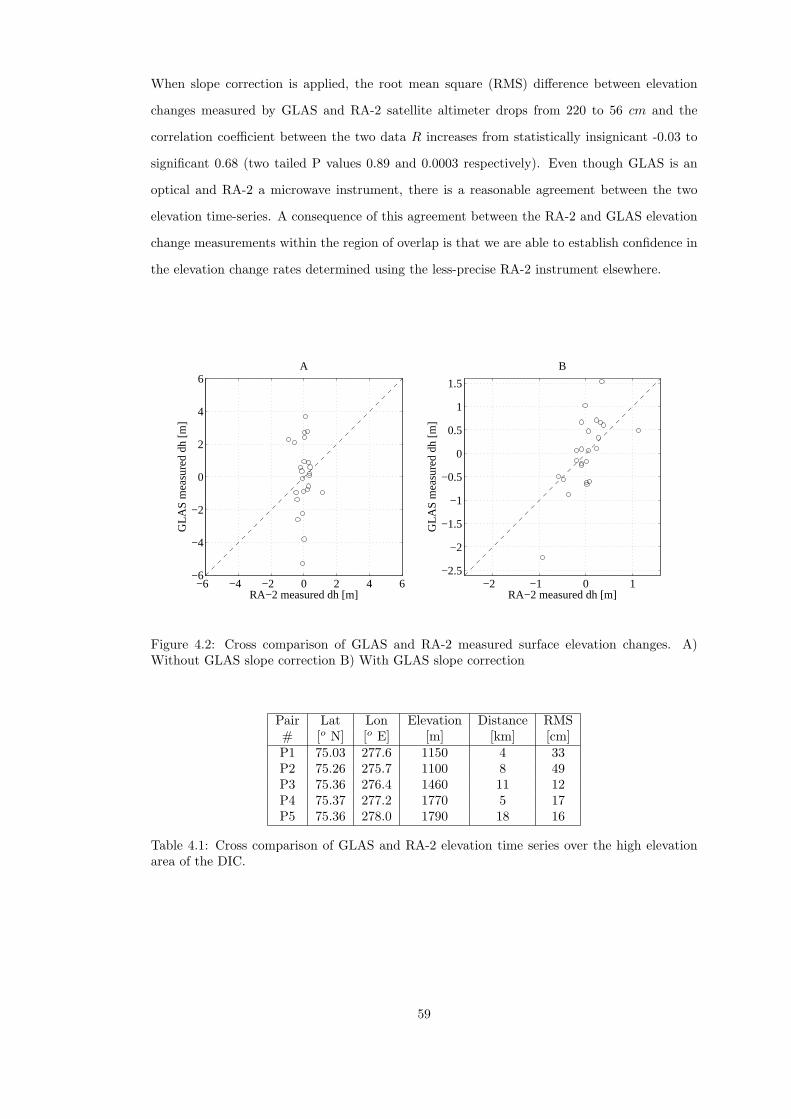
When slope correction is applied, the root mean square (RMS) difference between elevation
changes measured by GLAS and RA-2 satellite altimeter drops from 220 to 56 cm and the
correlation coefficient between the two data R increases from statistically insignicant -0.03 to
significant 0.68 (two tailed P values 0.89 and 0.0003 respectively). Even though GLAS is an
optical and RA-2 a microwave instrument, there is a reasonable agreement between the two
elevation time-series. A consequence of this agreement between the RA-2 and GLAS elevation
change measurements within the region of overlap is that we are able to establish confidence in
the elevation change rates determined using the less-precise RA-2 instrument elsewhere.
−2 −1 0 1−2.5
−2
−1.5
−1
−0.5
0
0.5
1
1.5
RA−2 measured dh [m]
GLA
S m
easu
red
dh [m
]
B
−6 −4 −2 0 2 4 6−6
−4
−2
0
2
4
6
RA−2 measured dh [m]
GLA
S m
easu
red
dh [m
]
A
Figure 4.2: Cross comparison of GLAS and RA-2 measured surface elevation changes. A)Without GLAS slope correction B) With GLAS slope correction
Pair Lat Lon Elevation Distance RMS# [o N] [o E] [m] [km] [cm]P1 75.03 277.6 1150 4 33P2 75.26 275.7 1100 8 49P3 75.36 276.4 1460 11 12P4 75.37 277.2 1770 5 17P5 75.36 278.0 1790 18 16
Table 4.1: Cross comparison of GLAS and RA-2 elevation time series over the high elevationarea of the DIC.
59
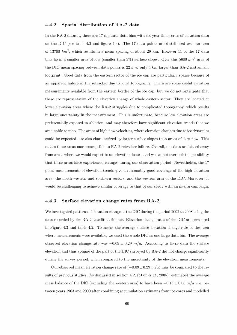
4.4.2 Spatial distribution of RA-2 data
In the RA-2 dataset, there are 17 separate data bins with six-year time-series of elevation data
on the DIC (see table 4.2 and figure 4.3). The 17 data points are distributed over an area
of 13700 km2, which results in a mean spacing of about 29 km. However 11 of the 17 data
bins lie in a smaller area of low (smaller than 3%) surface slope . Over this 5600 km2 area of
the DIC mean spacing between data points is 22 km: only 4 km larger than RA-2 instrument
footprint. Good data from the eastern sector of the ice cap are particularly sparse because of
an apparent failure in the retracker due to local topography. There are some useful elevation
measurements available from the eastern border of the ice cap, but we do not anticipate that
these are representative of the elevation change of whole eastern sector. They are located at
lower elevation areas where the RA-2 struggles due to complicated topography, which results
in large uncertainty in the measurement. This is unfortunate, because low elevation areas are
preferentially exposed to ablation, and may therefore have significant elevation trends that we
are unable to map. The areas of high flow velocities, where elevation changes due to ice dynamics
could be expected, are also characterized by larger surface slopes than areas of slow flow. This
makes these areas more susceptible to RA-2 retracker failure. Overall, our data are biased away
from areas where we would expect to see elevation losses, and we cannot overlook the possibility
that these areas have experienced changes during our observation period. Nevertheless, the 17
point measurements of elevation trends give a reasonably good coverage of the high elevation
area, the north-western and southern sectors, and the western arm of the DIC. Moreover, it
would be challenging to achieve similar coverage to that of our study with an in-situ campaign.
4.4.3 Surface elevation change rates from RA-2
We investigated patterns of elevation change at the DIC during the period 2002 to 2008 using the
data recorded by the RA-2 satellite altimeter. Elevation change rates of the DIC are presented
in Figure 4.3 and table 4.2. To assess the average surface elevation change rate of the area
where measurements were available, we used the whole DIC as one large data bin. The average
observed elevation change rate was −0.09 ± 0.29 m/a. According to these data the surface
elevation and thus volume of the part of the DIC surveyed by RA-2 did not change significantly
during the survey period, when compared to the uncertainty of the elevation measurements.
Our observed mean elevation change rate of (−0.09±0.29 m/a) may be compared to the re-
sults of previous studies. As discussed in section 4.2, (Mair et al., 2005). estimated the average
mass balance of the DIC (excluding the western arm) to have been −0.13± 0.06 m/a w.e. be-
tween years 1963 and 2000 after combining accumulation estimates from ice cores and modelled
60
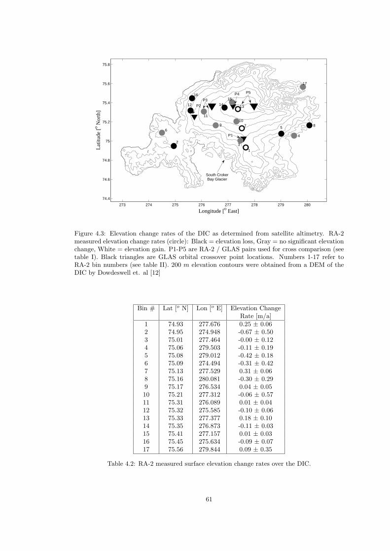
Longitude [o East]
Latit
ude
[o Nor
th]
1
23
4
56
7 8910
11
12 1314
1516
17
273 274 275 276 277 278 279 280
74.4
74.6
74.8
75
75.2
75.4
75.6
75.8
P1
P4
P3
P5
P2
South CrokerBay Glacier
Figure 4.3: Elevation change rates of the DIC as determined from satellite altimetry. RA-2measured elevation change rates (circle): Black = elevation loss, Gray = no significant elevationchange, White = elevation gain. P1-P5 are RA-2 / GLAS pairs used for cross comparison (seetable I). Black triangles are GLAS orbital crossover point locations. Numbers 1-17 refer toRA-2 bin numbers (see table II). 200 m elevation contours were obtained from a DEM of theDIC by Dowdeswell et. al [12]
Bin # Lat [o N] Lon [o E] Elevation ChangeRate [m/a]
1 74.93 277.676 0.25 ± 0.062 74.95 274.948 -0.67 ± 0.503 75.01 277.464 -0.00 ± 0.124 75.06 279.503 -0.11 ± 0.195 75.08 279.012 -0.42 ± 0.186 75.09 274.494 -0.31 ± 0.427 75.13 277.529 0.31 ± 0.068 75.16 280.081 -0.30 ± 0.299 75.17 276.534 0.04 ± 0.0510 75.21 277.312 -0.06 ± 0.5711 75.31 276.089 0.01 ± 0.0412 75.32 275.585 -0.10 ± 0.0613 75.33 277.377 0.18 ± 0.1014 75.35 276.873 -0.11 ± 0.0315 75.41 277.157 0.01 ± 0.0316 75.45 275.634 -0.09 ± 0.0717 75.56 279.844 0.09 ± 0.35
Table 4.2: RA-2 measured surface elevation change rates over the DIC.
61
melt of the ice cap. Shepherd et al. (2007) combined model estimates of surface mass balance
with ice surface velocities derived from InSAR data from 1996, and estimated that the mass
balance of the main DIC was −1.08±0.66 km3/a w.e. (equivalent to an average elevation change
rate of −0.09±0.05 m/a w.e.). (Burgess & Sharp, 2008) estimated the average mass balance of
the DIC to have been −76.8 ± 7km3 between 1963 and 2000 corresponding to mean elevation
change rate of −0.17 ± 0.02 m/a w.e. Their estimate was based on a study similar to Mair
et al. (2005) and Shepherd et al. (2007) but they also utilized ice velocity measurements from
multiple sources including in-situ stake measurements and InSAR. Although our estimate of
the DIC elevation change is biased due to limited coverage and equivocal, given the large degree
of uncertainty, it is consistent with the findings of the previous studies which have concluded
that the ice cap is losing mass. Factors, such as potential fluctuations in the ice cap density,
data omission and temporal sampling of the data, may also contribute towards differences be-
tween the observed elevation trend and the results of previous studies. Good RA-2 data, for
example, were scarce in the eastern sector of the DIC – a region that previous studies (Mair
et al. (2005) and Burgess & Sharp (2008)) have consistently found to be losing mass – and so
our measurement of changes in the ice cap elevation may underestimate the overall trend. Our
estimate of the overall elevation change rate is biased towards sampling flat areas which exhibit
little or no significant elevation change. Finally, our study period was 2002-2008, whereas all
of the previous studies of the DIC mass change based their estimate either completely (Mair
et al., 2005) or partially (Colgan et al. (2008), Shepherd et al. (2007) and Burgess & Sharp
(2008)) on data acquired during the late 20th century.
The RA-2 data (Figure 4.3) also show considerable regional variation in the rate of elevation
change across the ice cap. According to our data, the elevation of the high altitude area (bins
13, 14 and 15) and north-western sector (bins 9, 11, 12 and 16, see also subsection 4.4.4) did
not change substantially during our observation period. The eastern sector (bin 5) and the
western arm (bin 2 and 6) decreased in elevation whereas the southern sector (bins 1, 3, 7 and
10) gained elevation. Our data from high-elevation areas agree well with the previous estimates.
Colgan et al. (2008) found a near-zero net elevation change of 0.01± 0.12 m/a w.e. for regions
above 1200 m. NASA repeat airborne laser survey by Abdalati et al. (2004), the only previous
study of DIC directly comparable with ours, found a near-zero or a small positive trend across
the high elevation area between 1995 and 2000. Our observation that the eastern sector was
losing elevation between 2002 and 2008 is in good agreement with the findings of Mair et al.
(2005), Shepherd et al. (2007), Burgess & Sharp (2008) and Colgan et al. (2008), which all agree
this sector is losing mass. Our observed elevation change of north-western sector is discussed
62
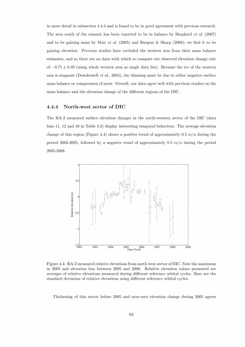
in more detail in subsection 4.4.4 and is found to be in good agreement with previous research.
The area south of the summit has been reported to be in balance by Shepherd et al. (2007)
and to be gaining mass by Mair et al. (2005) and Burgess & Sharp (2008); we find it to be
gaining elevation. Previous studies have excluded the western arm from their mass balance
estimates, and so there are no data with which to compare our observed elevation change rate
of −0.71 ± 0.49 (using whole western arm as single data bin). Because the ice of the western
arm is stagnant (Dowdeswell et al., 2004), the thinning must be due to either negative surface
mass balance or compression of snow. Overall, our data agree well with previous studies on the
mass balance and the elevation change of the different regions of the DIC.
4.4.4 North-west sector of DIC
The RA-2 measured surface elevation changes in the north-western sector of the DIC (data
bins 11, 12 and 16 in Table 4.2) display interesting temporal behaviour. The average elevation
change of this region (Figure 4.4) shows a positive trend of approximately 0.5 m/a during the
period 2002-2005, followed by a negative trend of approximately 0.5 m/a during the period
2005-2008.
2002 2003 2004 2005 2006 2007 2008 2009−1.5
−1
−0.5
0
0.5
1
Time [Year]
Rel
ativ
e el
evat
ion
[m]
Figure 4.4: RA-2 measured relative elevations from north west sector of DIC. Note the maximumin 2005 and elevation loss between 2005 and 2008. Relative elevation values presented areaverages of relative elevations measured during different reference orbital cycles. Bars are thestandard deviation of relative elevations using different reference orbital cycles.
Thickening of this sector before 2005 and near-zero elevation change during 2005 agrees
63
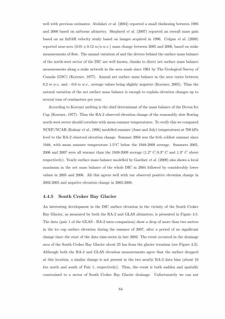
well with previous estimates: Abdalati et al. (2004) reported a small thickening between 1995
and 2000 based on airborne altimetry. Shepherd et al. (2007) reported an overall mass gain
based on an InSAR velocity study based on images acquired in 1996. Colgan et al. (2008)
reported near-zero (0.01± 0.12 m/a w.e.) mass change between 2005 and 2006, based on stake
measurements of flow. The annual variation of and the drivers behind the surface mass balance
of the north-west sector of the DIC are well known, thanks to direct net surface mass balance
measurements along a stake network in the area made since 1961 by The Geological Survey of
Canada (GSC) (Koerner, 1977). Annual net surface mass balance in the area varies between
0.2 m w.e. and −0.6 m w.e., average values being slightly negative (Koerner, 2005). Thus the
natural variation of the net surface mass balance is enough to explain elevation changes up to
several tens of centimeters per year.
According to Koerner melting is the chief determinant of the mass balance of the Devon Ice
Cap (Koerner, 1977). Thus the RA-2 observed elevation change of the reasonably slow flowing
north-west sector should correlate with mean summer temperatures. To verify this we compared
NCEP/NCAR (Kalnay et al., 1996) modelled summer (June and July) temperatures at 700 hPa
level to the RA-2 observed elevation change. Summer 2004 was the 6:th coldest summer since
1948, with mean summer temperature 1.5oC below the 1948-2009 average. Summers 2005,
2006 and 2007 were all warmer than the 1949-2009 average (1.2o C, 0.3o C and 1.3o C above
respectively). Yearly surface mass balance modelled by Gardner et al. (2009) also shows a local
maximum in the net mass balance of the whole DIC in 2004 followed by considerably lower
values in 2005 and 2006. All this agrees well with our observed positive elevation change in
2002-2005 and negative elevation change in 2005-2008.
4.4.5 South Croker Bay Glacier
An interesting development in the DIC surface elevation in the vicinity of the South Croker
Bay Glacier, as measured by both the RA-2 and GLAS altimeters, is presented in Figure 4.5.
The data (pair 1 of the GLAS - RA-2 inter-comparison) show a drop of more than two meters
in the ice cap surface elevation during the summer of 2007, after a period of no significant
change since the start of the data time-series in late 2003. The event occurred in the drainage
area of the South Croker Bay Glacier about 25 km from the glacier terminus (see Figure 4.3).
Although both the RA-2 and GLAS elevation measurements agree that the surface dropped
at this location, a similar change is not present in the two nearby RA-2 data bins (about 10
km north and south of Pair 1, respectively). Thus, the event is both sudden and spatially
constrained to a sector of South Croker Bay Glacier drainage. Unfortunately we can not
64
constrain the extent of the event in the East-West direction with available RA-2 data. Shepherd
et. al estimated the accumulation in this region to be approximately 0.30 m/a w.e. (Shepherd
et al., 2007) – an order of magnitude smaller than our observed elevation drop. This suggests
that the decrease is not likely related to an accumulation shortfall. The signal is more easily
explained as a rapid dynamic process. Because similar behaviour is not seen in the nearby
data bins we propose that the drop is connected with a local change in the ice cap dynamics.
Although verification of this hypothesis would require independent velocity measurements from
the area (either in-situ or from satellite observations) from early- and late-2007, there is some
evidence of rapid dynamic changes in this sector of the DIC. Burgess and Sharp measured
considerable thinning up to 2 m/a at elevations lower than 400 m at the South Croker Bay
Glacier during 2004 and 2005 (Burgess & Sharp, 2008), and they also suggest the thinning is
probably driven by recent changes in ice dynamics.
2002 2003 2004 2005 2006 2007 2008 2009−2.5
−2
−1.5
−1
−0.5
0
0.5
1
1.5
Time [Year]
Rel
ativ
e el
evat
ion
[m]
ICESat GLAS
EnviSAT RA−2
Figure 4.5: Surface elevation development of RA-2 / GLAS comparison pair 1, South CrokerBay drainage area. RA-2 error estimates are the standard deviations of relative elevations usingdifferent reference orbital cycles. GLAS error estimate is the 14 cm pre-launch RSS single-shoterror estimate by Zwally et al. (2002).
4.5 Conclusions
For the first time, we have combined satellite laser and radar altimeter data to assess the surface
elevation change of an ice cap – the Devon Ice Cap in northern Canada – an ice body consider-
ably smaller than the continental ice sheets where such methods traditionally have been applied
65
(Slobbe et al. (2008), Smith et al. (2005), Davis & Ferguson (2004), Wingham et al. (1998) and
Howat et al. (2008)). Despite the small target size, we have obtained results that are in line
with previous research (Mair et al. (2005), Shepherd et al. (2007), Burgess & Sharp (2008),
Colgan et al. (2008) and Abdalati et al. (2004)). What’s more, where coincident laser and
radar altimeter measurements from independent satellites are available, they agree to a satis-
factory extent (RMS difference = 56 cm and R = 0.68.). We have shown the average elevation
change trend of the parts of the DIC covered by RA-2 measurements (the high elevation area,
western arm, north-western and southern sectors as well as some parts of the eastern sector)
to have been −0.09± 0.29 m/a between the years 2002 and 2008. There are, however, detailed
differences between sub-basins of the ice cap: some are thickening and some thinning.
The DIC western arm is shown to have thinned, most likely due to a negative surface mass
balance. We have observed a change in sign of the ice cap elevation trend in the north-western
sector: according to our data, this area – previously estimated to be in balance (Colgan et al.,
2008) or thickening (Abdalati et al. (2004) and Shepherd et al. (2007)) – was thinning between
years 2005 and 2008. This thinning is likely due to high melt induced by warm summers in the
area during these years.
We have observed a sudden 2 m drop in the elevation of the South Croker Bay Glacier
drainage area during the summer 2007. The drop is apparent in both the GLAS and RA-2
satellite altimeter datasets and is an order of magnitude greater than the annual accumulation
rate, suggesting its origins are more likely related to a dynamic event. This is the first time
that RA-2 has been employed to observe such a spatially small event.
Our algorithms for processing elevation changes using both RA-2 and GLAS satellite altime-
ter data can be readily adapted to study elevation changes of other large ice caps. In addition,
the RA-2 algorithm is automatic, and does not require additional data. Due to certain limita-
tions of the GLAS dataset, including the lack of overlapping ground tracks in different years, an
external DEM of the target substantially improves the certainty of estimates of ice cap elevation
change.
4.6 Acknowledgements
The authors would like to thank the anonymous reviewers for their valuable comments to
improve the manuscript.
66
Chapter 5
On the Recent Elevation Changes
at the Flade Isblink Ice Cap,
Northern Greenland
This chapter describes the recent surface elevation changes of the Flade Isblink Ice Cap and compares
altimeter measurements to modelled SMB values. This chapter has been published as “On the Recent
Elevation Changes at the Flade Isblink Ice Cap, Northern Greenland”
Authors: Rinne, E.; Shepherd, A.; Palmer, S.; van den Broeke M.R.; Muir A.; Ettema J.; Wing-
ham D.
Appears in: Journal of Geophysical Research – Earth Surface
Digital Object Identifier: 10.1029/2011JF001972
Date of Publication: 21 September 2011
I processed the altimeter data from GLAS level 2 and RA-2 crossover elevation differences onwards.
The RA-2 crossover processing was done by Muir. I compared the altimeter data to modelled SMB
values. I interpreted the results and wrote most of the manuscript. Shepherd provided the original
research idea, assisted with the interpretation of the data and writing the manuscript. Palmer provided
the DEM required for GLAS slope correction and assisted with writing the manuscript. Both Van den
Broeke and Ettema provided the RACMO2 SMB data and Van den Broeke wrote the text concerning
RACMO2 in the methodology section of the manuscript.
67
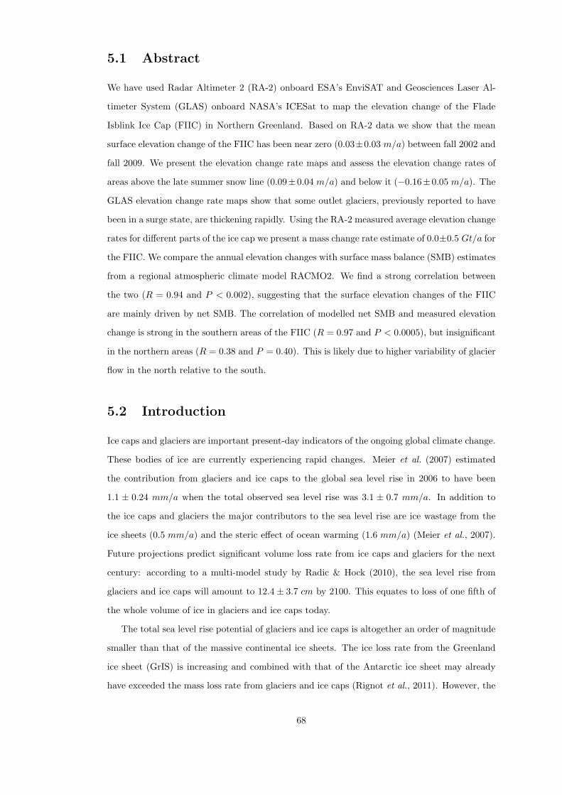
5.1 Abstract
We have used Radar Altimeter 2 (RA-2) onboard ESA’s EnviSAT and Geosciences Laser Al-
timeter System (GLAS) onboard NASA’s ICESat to map the elevation change of the Flade
Isblink Ice Cap (FIIC) in Northern Greenland. Based on RA-2 data we show that the mean
surface elevation change of the FIIC has been near zero (0.03±0.03 m/a) between fall 2002 and
fall 2009. We present the elevation change rate maps and assess the elevation change rates of
areas above the late summer snow line (0.09±0.04 m/a) and below it (−0.16±0.05 m/a). The
GLAS elevation change rate maps show that some outlet glaciers, previously reported to have
been in a surge state, are thickening rapidly. Using the RA-2 measured average elevation change
rates for different parts of the ice cap we present a mass change rate estimate of 0.0±0.5 Gt/a for
the FIIC. We compare the annual elevation changes with surface mass balance (SMB) estimates
from a regional atmospheric climate model RACMO2. We find a strong correlation between
the two (R = 0.94 and P < 0.002), suggesting that the surface elevation changes of the FIIC
are mainly driven by net SMB. The correlation of modelled net SMB and measured elevation
change is strong in the southern areas of the FIIC (R = 0.97 and P < 0.0005), but insignificant
in the northern areas (R = 0.38 and P = 0.40). This is likely due to higher variability of glacier
flow in the north relative to the south.
5.2 Introduction
Ice caps and glaciers are important present-day indicators of the ongoing global climate change.
These bodies of ice are currently experiencing rapid changes. Meier et al. (2007) estimated
the contribution from glaciers and ice caps to the global sea level rise in 2006 to have been
1.1 ± 0.24 mm/a when the total observed sea level rise was 3.1 ± 0.7 mm/a. In addition to
the ice caps and glaciers the major contributors to the sea level rise are ice wastage from the
ice sheets (0.5 mm/a) and the steric effect of ocean warming (1.6 mm/a) (Meier et al., 2007).
Future projections predict significant volume loss rate from ice caps and glaciers for the next
century: according to a multi-model study by Radic & Hock (2010), the sea level rise from
glaciers and ice caps will amount to 12.4± 3.7 cm by 2100. This equates to loss of one fifth of
the whole volume of ice in glaciers and ice caps today.
The total sea level rise potential of glaciers and ice caps is altogether an order of magnitude
smaller than that of the massive continental ice sheets. The ice loss rate from the Greenland
ice sheet (GrIS) is increasing and combined with that of the Antarctic ice sheet may already
have exceeded the mass loss rate from glaciers and ice caps (Rignot et al., 2011). However, the
68
contribution of ice caps and glaciers will stay significant during the next century. Also, because
systems of different size will react differently to rising global temperatures, the study of all land
ice bodies is vital in the context of global warming.
The surface mass balance (SMB) of an ice cap is determined by climate, mostly by pre-
cipitation and surface energy balance. These govern the rates of accumulation and ablation,
respectively. A change in climate affects the rates of snow accumulation and ablation of the
ice caps which, in turn, may lead to changes in their surface elevation. Other processes, such
as iceberg calving and changes in ice and snow density, will also have an effect on the ice cap
surface elevation.
Recent satellite altimeters, such as the Radar Altimeter 2 (RA-2) (Resti et al., 1999b) and
the Geosciences Laser Altimeter System (GLAS) (Zwally et al., 2002), provide near-global data
sets of surface elevation. These data can be applied to surface elevation change studies of
land ice masses. Satellite measurements provide extensive spatial and temporal coverage of the
remote and rarely visited areas, that in practice cannot be monitored by other means.
Flade Isblink Ice Cap (FIIC) is located in North-East Greenland (Figure 5.1). It covers
an area of 8500 km2, which makes it the largest ice cap in Greenland separate from the GrIS
(Kelly & Lowell, 2009). The FIIC is characterized by low surface slopes in its north-east
part, and steeper slopes as well as some nunataks in the south-west part, which overlays the
Princess Elisabeth Alps. The maximum elevation of the FIIC is approximately 960 m and
the ice thickness close to the central summit is 535 m. The weather patterns of the FIIC are
controlled by moisture and heat from the ice-free ocean to the east, and cold dry winds from the
north-west (Rasmussen, 2004). The FIIC forces the cold north-westerly air mass upwards into
the warmer moist air mass originating from the ice-free eastern side. When these air masses
meet, precipitation falls on the western side of the FIIC, while the eastern side is sheltered and
receives less snow (Rasmussen, 2004).
The outlet glaciers of the FIIC have experienced several advances and retreats. Radiocarbon
dating of glacially overrun sediments show that the FIIC glaciers advanced sometime after 7800
BP, but have retreated since (Hjort, 1997). Some model studies suggest the present-day FIIC
to be a young ice mass – only some thousands of years old, much like the Hans Tausen Ice
Cap to the west of the FIIC (Lemark, 2009). Plant remains dated to 1510-1600 AD were also
found to have been overrun by the margin of the FIIC, suggesting that the FIIC has advanced
as recently as during the Little Ice Age (Hjort, 1997).
There have been two previous studies describing surface elevation changes at the FIIC
[Krabill et al. (2000) and Pritchard et al. (2009)]. Both of these studies concentrated on the
69
Figure 5.1: Location and map of the FIIC. South and North domes combined are the flat areaof surface slopes < 3%
GrIS, but they also included elevation change estimates for the FIIC. Krabill et al. (2000)
conducted aircraft laser altimeter campaigns in Greenland for the years 1994 and 1999. Their
repeat measurements along two intersecting flight lines over the FIIC show a thickening of
0.4− 0.6 m/a across most of the ice cap surface, with a small area of thinning near the eastern
margin. The fastest thickening was observed in the south-western part of the FIIC (Krabill
et al., 2000). Pritchard et al. (2009) used the GLAS to examine elevation changes of the GrIS,
but also included the FIIC in their study domain. They found that between 2003 and 2007, the
western half of the FIIC thickened by around 0.5 m/a and the eastern half thinned by around
0.2 m/a. Because the main target of both studies was the GrIS, the chosen spatial resolution of
their elevation change maps did not resolve the details of the FIIC elevation changes [Pritchard
et al. (2009) and Krabill et al. (2000)].
In this paper we assess the elevation change of the FIIC for the years 2002 to 2009 using
two satellite altimeters: RA-2 and GLAS. Maps of the elevation change rates of the FIIC
are presented for the time period 2004-2008. We also compare annual RA-2 elevation change
measurements with the modelled net SMB estimates from the regional climate model RACMO2.
This way we can assess the recent mass changes of FIIC, as well as the role and importance of
SMB in the evolution of FIIC surface elevation.
70
5.3 Methodology
To assess the elevation change of FIIC we used two independent satellite altimeters: GLAS
that flew with NASA’s Ice, Cloud and land Elevation satellite (ICESat) (Zwally et al., 2002),
and RA-2 flying onboard ESA’s Environmental satellite (EnviSAT) (Resti et al., 1999b). The
two altimeters operate at different frequencies, GLAS being a laser altimeter and RA-2 a radar
altimeter. They complement each other in both temporal and spatial resolution. The RA-2
has a large beam-limited footprint of 19 km (Resti et al., 1999b). Although the pulse-limited
ground footprint of RA-2 is considerably smaller than this (Soussi & Femenias, 2006), the
spatial resolution of RA-2 is still two orders of magnitude poorer than that of GLAS, which
has a footprint of only about 70 m (Zwally et al., 2002). The advantage of RA-2 is that it
provides measurements independent of cloud conditions, whereas clouds limited the GLAS data
aquisition. Furthermore, GLAS only obtained measurements during two or three periods per
year. At a given point under an ICESat ground track on the FIIC, there were on average 4.1
successful GLAS measurements during 2004-2008. For the same period, the RA-2 provided an
average of 31.9 successful measurements per crossover point on the FIIC.
5.3.1 ICESat GLAS
GLAS provided near global (86oN to 86oS latitude) surface elevation measurements from Febru-
ary 2003 until the failure of the last laser in October 2009. One of the major challenges in
obtaining elevation change estimates from GLAS data is the local cross-track slope estimate
requirement. The ground tracks of ICESat from different years may have a spacing of up to
100 m at the FIIC. As a result, even a reasonably small cross-track slope of 2% creates a 2 m
difference in elevations measured during different tracks. This is larger than the expected ele-
vation change signal, and therefore the effect of the cross-track slope has to be removed from
the measured elevation values.
A method to estimate the cross-track slope, known as plane fitting, was used by Pritchard
et al. (2009). They calculated the average cross-track slope for all measured track pairs during
2003, and used this to compensate for surface slope in later measurements. For our slope
correction we use a high precision (better than 10 cm) digital elevation model (DEM), formed
using interferometric synthetic aperture radar (InSAR) data acquired by the European Remote
Sensing (ERS) satellite in winter 1996 (Palmer et al., 2010). As InSAR-derived height maps
contain relative values only, absolute surface elevation can only be retrieved with the use of tie-
points of known elevation (Nielsen et al., 1997). For the FIIC DEM this retrieval is achieved by
71
applying a least-squares fit of the unwrapped phase at 500 points of known elevation, measured
by GLAS in 2007 (Palmer et al., 2010). Thus the FIIC DEM we utilize is not independent of
the GLAS data used in this study. However, in our analysis of GLAS data we only use the
slope information from the DEM and not the absolute height. Therefore the dependence of
FIIC DEM on GLAS data does not impede the quality of our elevation change estimates.
The GLAS data used in this paper is the GLAS/ICESat L1B Global Elevation Dataset or
GLA06, available free of charge online from the National Snow and Ice Data Center (NSIDC)
(Zwally et al., 2003). Saturation correction was added to the elevations. Data points with no
saturation elevation correction or large receiver gain values (greater than 150) were discarded.
Geolocations in the GLA06 dataset were used without additional corrections.
To assess the elevation change of the ice surface, we calculated the difference (∆h(x, t))
between GLAS measured elevations h(x, t) and our DEM (hDEM ). Both the GLAS measured
and DEM elevations were in reference to the ICESat/GLAS geoid. We calculated the average
∆h(x, t) for x inside 1km2 data bins for each operations period:
∆h(x, t) =
∑ni=1
hi(x, t)− hDEM (x)
n(5.1)
If the local features present in the GLAS data are resolved by the DEM, the ∆h is the
sum of three factors: error in DEM (for example due to radar penetration), GLAS instrument
error, and actual physical changes in surface elevation between the time of the InSAR study
and the GLAS measurement. To obtain an elevation trend, we fitted a first degree polynomial
to these elevation differences, so that the slope of the polynomial represents the elevation trend
in the data bin. For the elevation trend map, the elevation trends were then interpolated by a
bicubic spline method (Sandwell, 1987) to obtain elevation trends between ICESat tracks where
no measurements were available. Average elevation trends for large areas were calculated from
non-interpolated measurements.
We did not calculate a formal error estimate for each elevation measurement, because too
many of the contributory factors (surface roughness, change of the surface topography since
the DEM was measured, etc.) are poorly known. Instead we use the 1-σ confidence interval
provided by the regression of the trend. Similar error estimate based on variation of the elevation
measurements has been used in the past for example by Wingham et al. (1998). There is a
known GLAS inter-campaign bias that adds a systematic error to measured elevation change
rates. Magnitude of the trend of this bias has been estimated to be of the order of 0.006 m/a
by Zwally et al. (2011). Due to this error contribution, we added 0.01 m/a to our GLAS
uncertainty estimates.
72
5.3.2 EnviSAT RA-2
To assess the elevation change rate from RA-2, we employed the dual crossover method pre-
viously used to assess the elevation change of the Antarctic Ice Sheet (Wingham et al., 1998),
GrIS (Thomas et al., 2008) and the Devon Ice Cap (Rinne et al., 2011). The method is based
on the dh/dt -method introduced by Zwally et al. (1989). In the dual crossover method only
crossovers with two pairs of tracks (see Equation 5.2) are used.
The foundation of our RA-2 processing is to define the change in elevation, ∆h(x, t, tref ),
in orbital crossover points x between times t and tref :
∆h(x, t, tref ) =
[
(hAt − hDtref )− (hAtref − hDt)
2
]
t=t1...tN
(5.2)
hAt and hDt refer to elevations measured during ascending and descending passes, respec-
tively. Using the average of two different geometry crossovers removes the possible ascend-
ing versus descending biases in radar penetration. In this manner, we get a time series of
∆h(x, t, tref ). To reduce noise, values of ∆h(x, t, tref ) are binned into 10 km by 10 km cells
(data bins) and then averaged.
The choice of the reference time tref affects the resulting time series ∆h(x, t, tref ). As we are
calculating the change in elevation, and not the absolute elevation, we can choose an arbitrary
point in time (within our measurement period) as our reference. In practice a choice of one
reference point in time is not enough, as a measurement from a certain point in time may lack
some coverage over the study area. Also there are errors inherent in every measurement, and
choosing just one reference point may introduce bias into the resulting time series.
Instead, we used ten different time periods (ten orbital cycles of 35 days) as references. We
assume the elevation change during one orbital cycle to be negligible. Every chosen reference
cycle yields a slightly different time series of ∆h(x, t, tref ). The time series using different
reference cycles were finally combined into one, which reduces the uncertainty and leads to a
better coverage of the study area.
The individual time series, in reference to different orbital cycles, have a different placement
regards to the level of zero elevation change. Before their combination, a constant value was
added to each time series. Adding this constant (which assumed a different value for each time
series) adjusted each time series so that it was in reference to the same level of zero elevation
change. The value of this constant was optimized so that the square sum of differences between
the time series (after adding the constant) and the time series with most data points was
minimized.
73
Finally, a first degree polynomial P∆h was fitted to the combined time series of ∆h(x, t)
in each bin. The slope of P∆h represents the elevation change rate dh/dt. The overall trend
is determined from the slope of a first degree polynomial, even if the elevation change of the
ice surface is not always linear. Although we could have used the difference of the first and
last elevation measurement (being analogous to two altimeter campaigns at different times),
our chosen method is less sensitive to error in single measurements or anomalous circumstances
during one of the measurements times.
The largest error sources contributing to the radar altimeter measurement are radar speckle
(associated with sub-footprint surface topography) and time-variant penetration of the radar
signal into the snow-pack (Arthern et al., 2001). To minimize the variation of radar penetration,
we only use RA-2 measurements from times when the snow surface is wet and the radar pene-
tration is negligible. Hall et al. (2008) compared satellite-based Moderate Resolution Imaging
Spectroradiometer (MODIS) measurements of surface temperature to in situ observations and
found that there was no variation in surface temperature with elevation on 3 July 2001 and on
23 June 2004, suggesting that the entire ice surface of the FIIC was at or near to melting on
these dates. We only use RA-2 measurements made between late summer and early fall (start
of July and mid-September).
Because we compared RA-2 measurements with other RA-2 measurements only, we did
not apply a slant-range correction. Furthermore, we chose not to apply the re-location of
measurement. Due to this, the actual location of radar echo is upslope from the nadir point.
In consequence, we can’t measure the very lowest elevations of the ice cap. All of the error
sources are functions of time and location and, in general, are poorly known – especially on an
ice surface with non-zero slopes. Analogously to GLAS, in the absence of formal estimates of
error for the RA-2 over ice caps, we use the 1-σ confidence interval provided by the regression
of the trend as our error estimate edh/dt.
5.3.3 RACMO2 climate model
The Regional Atmospheric Climate Model (RACMO2/GR) was applied over a domain that in-
cludes the GrIS and its surrounding oceans and islands at high horizontal resolution of 11 km.
For use over Greenland, RACMO2 has been coupled to a physical snow model that explicitly
treats properties of snow, firn and ice, meltwater percolation, retention and refreezing [Bouga-
mont & Bamber (2005) and Ettema et al. (2009)]. The atmospheric part of the model is forced
at the lateral boundaries and the sea surface by the interim-reanalysis of the ECMWF (Euro-
pean Centre for Medium-Range Weather Forecasts, ERA-Interim, 1989-2009). Ettema et al.
74
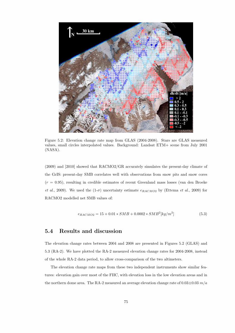
Figure 5.2: Elevation change rate map from GLAS (2004-2008). Stars are GLAS measuredvalues, small circles interpolated values. Background: Landsat ETM+ scene from July 2001(NASA).
(2009) and [2010] showed that RACMO2/GR accurately simulates the present-day climate of
the GrIS: present-day SMB correlates well with observations from snow pits and snow cores
(r = 0.95), resulting in credible estimates of recent Greenland mass losses (van den Broeke
et al., 2009). We used the (1-σ) uncertainty estimate eRACMO2 by (Ettema et al., 2009) for
RACMO2 modelled net SMB values of:
eRACMO2 = 15 + 0.01 ∗ SMB + 0.0002 ∗ SMB2[kg/m2] (5.3)
5.4 Results and discussion
The elevation change rates between 2004 and 2008 are presented in Figures 5.2 (GLAS) and
5.3 (RA-2). We have plotted the RA-2 measured elevation change rates for 2004-2008, instead
of the whole RA-2 data period, to allow cross-comparison of the two altimeters.
The elevation change rate maps from these two independent instruments show similar fea-
tures: elevation gain over most of the FIIC, with elevation loss in the low elevation areas and in
the northern dome area. The RA-2 measured an average elevation change rate of 0.03±0.03 m/a
75
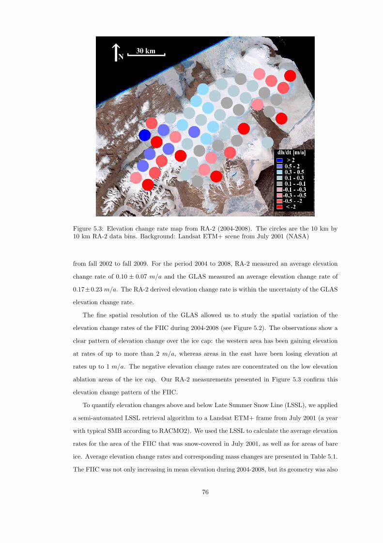
Figure 5.3: Elevation change rate map from RA-2 (2004-2008). The circles are the 10 km by10 km RA-2 data bins. Background: Landsat ETM+ scene from July 2001 (NASA)
from fall 2002 to fall 2009. For the period 2004 to 2008, RA-2 measured an average elevation
change rate of 0.10 ± 0.07 m/a and the GLAS measured an average elevation change rate of
0.17±0.23 m/a. The RA-2 derived elevation change rate is within the uncertainty of the GLAS
elevation change rate.
The fine spatial resolution of the GLAS allowed us to study the spatial variation of the
elevation change rates of the FIIC during 2004-2008 (see Figure 5.2). The observations show a
clear pattern of elevation change over the ice cap: the western area has been gaining elevation
at rates of up to more than 2 m/a, whereas areas in the east have been losing elevation at
rates up to 1 m/a. The negative elevation change rates are concentrated on the low elevation
ablation areas of the ice cap. Our RA-2 measurements presented in Figure 5.3 confirm this
elevation change pattern of the FIIC.
To quantify elevation changes above and below Late Summer Snow Line (LSSL), we applied
a semi-automated LSSL retrieval algorithm to a Landsat ETM+ frame from July 2001 (a year
with typical SMB according to RACMO2). We used the LSSL to calculate the average elevation
rates for the area of the FIIC that was snow-covered in July 2001, as well as for areas of bare
ice. Average elevation change rates and corresponding mass changes are presented in Table 5.1.
The FIIC was not only increasing in mean elevation during 2004-2008, but its geometry was also
76
changing: accumulation areas of the FIIC increased in elevation and ablation areas decreased in
elevation. Our elevation change rate map (Figure 5.2) agrees with the map of elevation change
rates by Pritchard et al. (2009) (using the same dataset but a different algorithm), but has a
better spatial resolution. Elevation change rates mapped by GLAS are also similar to those
mapped by a repeat airborne altimetry study in 1994 and 1999 (Krabill et al., 2000).
Closer inspection of the GLAS-measured elevation change reveals that three outlet glaciers
north-east of Station Nord gained elevation faster than the surrounding areas. Based on a study
of satellite measured velocities from 2000-2001 and 2005-2006, Joughin et al. (2010) reported
a large (from 300 m/a to 60 m/a) slowdown of the largest two of these glaciers. Several large
longitudinal crevasses and digitate termini, both characteristics of a surging glacier (Copland
et al., 2003), are visible in the Landsat ETM+ image acquired in July 2001. This implies that
the glaciers were in surge state during 2000, and that the surge had ended by 2005. Thickening
of these glaciers could be explained by slowdown in the glacier flow.
The drainage area of the northernmost glacier (northern dome) is also a notable exception
to the general pattern of increasing elevation at areas above the LSSL. Both GLAS and RA-2
measure an elevation loss in this area. The airborne study by Krabill et al. (2000) found this
area to have been thickening during 1994-1999, in a similar manner to other high elevation areas
of the FIIC. We suggest that the 2004-2008 decrease in the northern dome surface elevation
results from increased ice flow from the upper areas to the lower areas of the glacier after a
surge of the outlet glacier.
Based on the GLAS observations the thickening of some parts of the FIIC is among the
fastest in Greenland. The largest observed thickening rate on FIIC was 3.4 ± 0.7 m/a. In
addition to the peak thickening rate, a 1800 km2 area thickened faster than 0.5 m/a. Thick-
ening rates of this magnitude are not common on GrIS. Pritchard et al. (2009) found dynamic
thickening rates similar to those we have observed on FIIC only on two quiescent phase outlet
glaciers, Storsstrommen and L. Bistrup Brae, both in North-East Greenland. In contrast, thin-
ning rates we observe below the LSSL of FIIC are common in the margins of GrIS (Pritchard
et al., 2009).
To estimate the net mass change rate of the FIIC, we first calculated the average elevation
change rate for the area above the LSSL (5848 km2) and for the area below it (3001 km2)
(see Table 5.1). These rates were 0.09 ± 0.04 m/a and −0.16 ± 0.05 m/a, respectively. We
assume the elevation gain above the LSSL to be due to thickening firn (average density of
660± 250 kg/m3), and elevation loss below the LSSL to be due to loss of ice (average density
of 900 ± 10 kg/m3). The same density values were used by Gardner et al. (2011) to derive
77
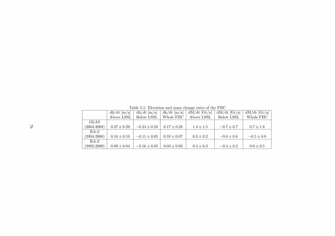
Table 5.1: Elevation and mass change rates of the FIICdh/dt [m/a] dh/dt [m/a] dh/dt [m/a] dM/dt [Gt/a] dM/dt [Gt/a] dM/dt [Gt/a]Above LSSL Below LSSL Whole FIIC Above LSSL Below LSSL Whole FIIC
GLAS(2004-2008) 0.27± 0.29 −0.24± 0.23 0.17± 0.28 1.4± 1.5 −0.7± 0.7 0.7± 1.8
RA-2(2004-2008) 0.16± 0.10 −0.11± 0.05 0.10± 0.07 0.3± 0.2 −0.8± 0.6 −0.5± 0.8
RA-2(2002-2009) 0.09± 0.04 −0.16± 0.05 0.03± 0.03 0.4± 0.3 −0.4± 0.2 0.0± 0.5
78
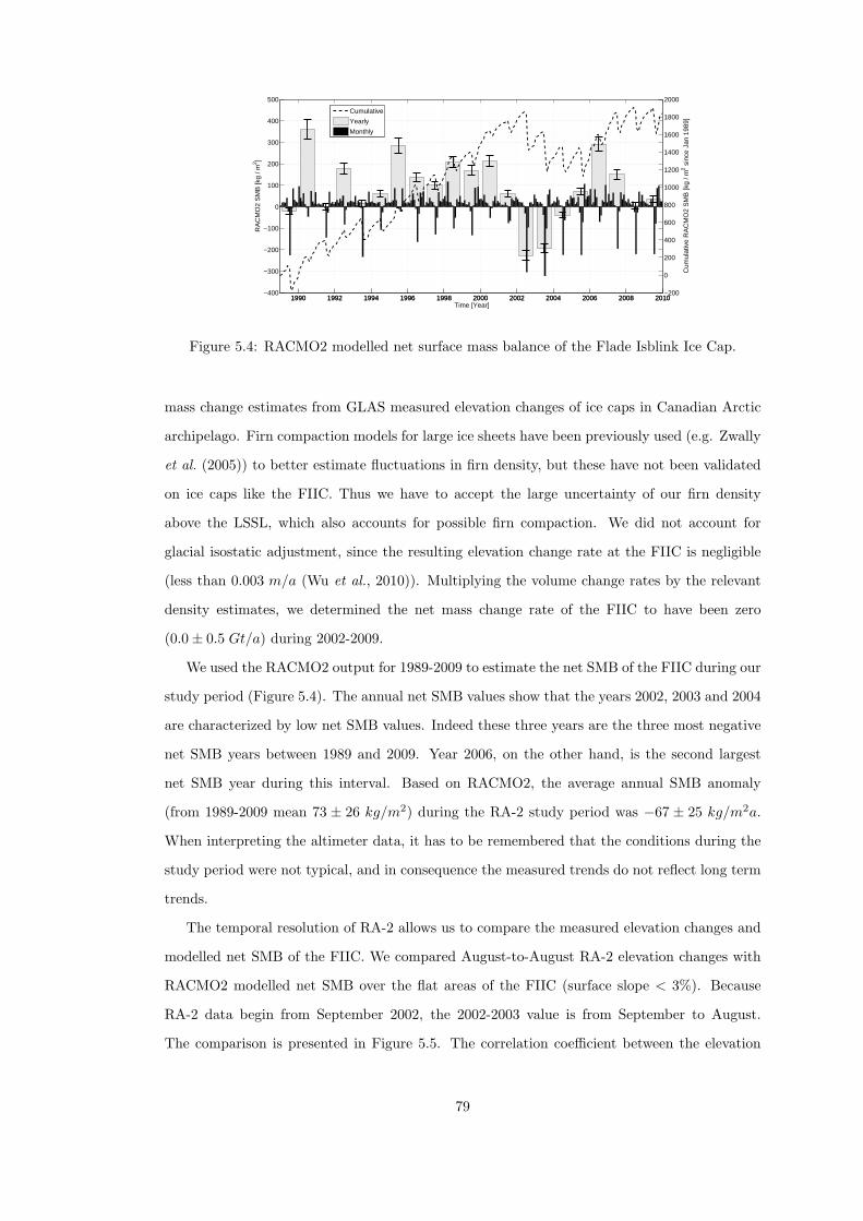
1990 1992 1994 1996 1998 2000 2002 2004 2006 2008 2010−400
−300
−200
−100
0
100
200
300
400
500
Time [Year]
RA
CM
O2
SM
B [k
g / m
2 ]
1990 1992 1994 1996 1998 2000 2002 2004 2006 2008 2010−200
0
200
400
600
800
1000
1200
1400
1600
1800
2000
Cum
ulat
ive
RA
CM
O2
SM
B [k
g / m
2 sin
ce J
an 1
989]
Cumulative
Yearly
Monthly
Figure 5.4: RACMO2 modelled net surface mass balance of the Flade Isblink Ice Cap.
mass change estimates from GLAS measured elevation changes of ice caps in Canadian Arctic
archipelago. Firn compaction models for large ice sheets have been previously used (e.g. Zwally
et al. (2005)) to better estimate fluctuations in firn density, but these have not been validated
on ice caps like the FIIC. Thus we have to accept the large uncertainty of our firn density
above the LSSL, which also accounts for possible firn compaction. We did not account for
glacial isostatic adjustment, since the resulting elevation change rate at the FIIC is negligible
(less than 0.003 m/a (Wu et al., 2010)). Multiplying the volume change rates by the relevant
density estimates, we determined the net mass change rate of the FIIC to have been zero
(0.0± 0.5 Gt/a) during 2002-2009.
We used the RACMO2 output for 1989-2009 to estimate the net SMB of the FIIC during our
study period (Figure 5.4). The annual net SMB values show that the years 2002, 2003 and 2004
are characterized by low net SMB values. Indeed these three years are the three most negative
net SMB years between 1989 and 2009. Year 2006, on the other hand, is the second largest
net SMB year during this interval. Based on RACMO2, the average annual SMB anomaly
(from 1989-2009 mean 73 ± 26 kg/m2) during the RA-2 study period was −67 ± 25 kg/m2a.
When interpreting the altimeter data, it has to be remembered that the conditions during the
study period were not typical, and in consequence the measured trends do not reflect long term
trends.
The temporal resolution of RA-2 allows us to compare the measured elevation changes and
modelled net SMB of the FIIC. We compared August-to-August RA-2 elevation changes with
RACMO2 modelled net SMB over the flat areas of the FIIC (surface slope < 3%). Because
RA-2 data begin from September 2002, the 2002-2003 value is from September to August.
The comparison is presented in Figure 5.5. The correlation coefficient between the elevation
79
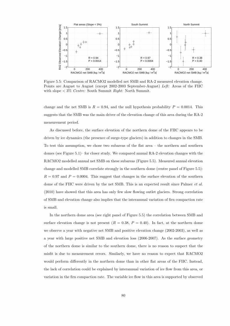
0 200 400−2
−1.5
−1
−0.5
0
0.5
1
1.5
RACMO2 net SMB [kg / m3a]
RA
2 O
bser
ved
Ele
vatio
n C
hang
e [m
/a] Flat areas (Slope < 3%)
R = 0.94P = 0.0014
0 200 400−2
−1.5
−1
−0.5
0
0.5
1
1.5
RACMO2 net SMB [kg / m3a]
South Summit
R = 0.97P = 0.0004
0 200 400−2
−1.5
−1
−0.5
0
0.5
1
1.5
RACMO2 net SMB [kg / m3a]
North Summit
R = 0.38P = 0.40
Figure 5.5: Comparison of RACMO2 modelled net SMB and RA-2 measured elevation change.Points are August to August (except 2002-2003 September-August) Left: Areas of the FIICwith slope < 3% Centre: South Summit Right: North Summit.
change and the net SMB is R = 0.94, and the null hypothesis probability P = 0.0014. This
suggests that the SMB was the main driver of the elevation change of this area during the RA-2
measurement period.
As discussed before, the surface elevation of the northern dome of the FIIC appears to be
driven by ice dynamics (the presence of surge-type glaciers) in addition to changes in the SMB.
To test this assumption, we chose two subareas of the flat area – the northern and southern
domes (see Figure 5.1)– for closer study. We compared annual RA-2 elevation changes with the
RACMO2 modelled annual net SMB on these subareas (Figure 5.5). Measured annual elevation
change and modelled SMB correlate strongly in the southern dome (centre panel of Figure 5.5):
R = 0.97 and P = 0.0004. This suggest that changes in the surface elevation of the southern
dome of the FIIC were driven by the net SMB. This is an expected result since Palmer et al.
(2010) have showed that this area has only few slow flowing outlet glaciers. Strong correlation
of SMB and elevation change also implies that the interannual variation of firn compaction rate
is small.
In the northern dome area (see right panel of Figure 5.5) the correlation between SMB and
surface elevation change is not present (R = 0.38, P = 0.40). In fact, at the northern dome
we observe a year with negative net SMB and positive elevation change (2002-2003), as well as
a year with large positive net SMB and elevation loss (2006-2007). As the surface geometry
of the northern dome is similar to the southern dome, there is no reason to suspect that the
misfit is due to measurement errors. Similarly, we have no reason to expect that RACMO2
would perform differently in the northern dome than in other flat areas of the FIIC. Instead,
the lack of correlation could be explained by interannual variation of ice flow from this area, or
variation in the firn compaction rate. The variable ice flow in this area is supported by observed
80
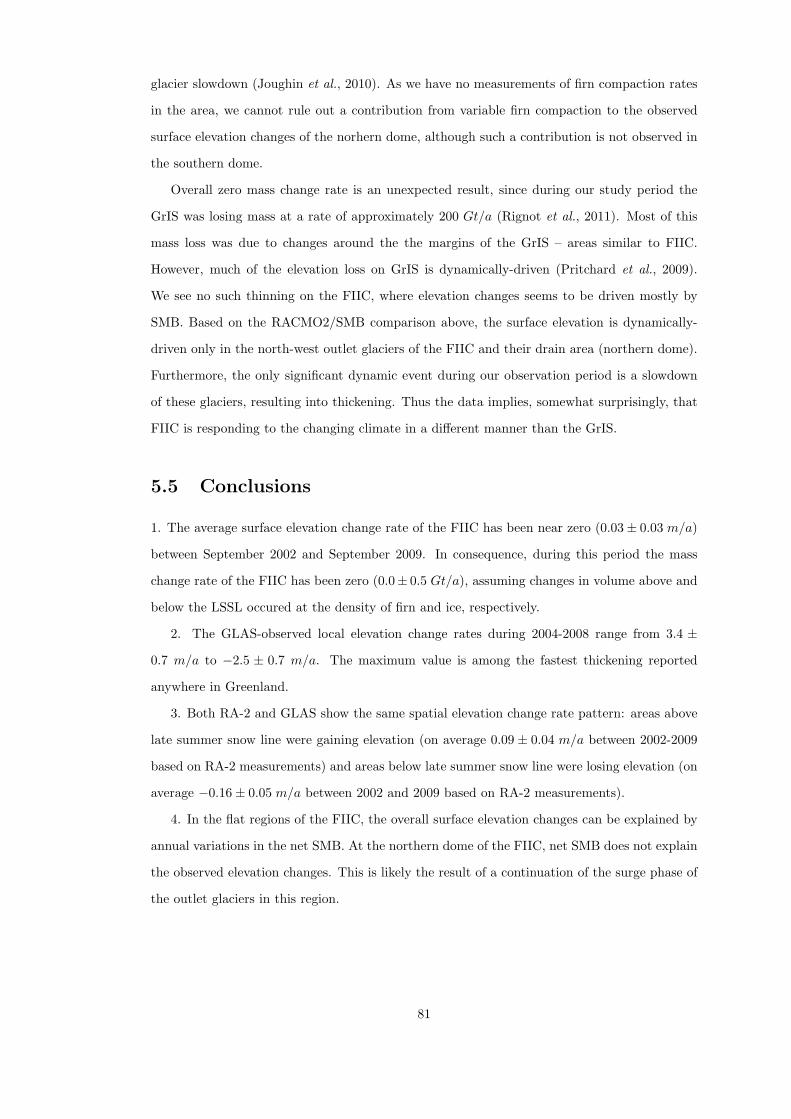
glacier slowdown (Joughin et al., 2010). As we have no measurements of firn compaction rates
in the area, we cannot rule out a contribution from variable firn compaction to the observed
surface elevation changes of the norhern dome, although such a contribution is not observed in
the southern dome.
Overall zero mass change rate is an unexpected result, since during our study period the
GrIS was losing mass at a rate of approximately 200 Gt/a (Rignot et al., 2011). Most of this
mass loss was due to changes around the the margins of the GrIS – areas similar to FIIC.
However, much of the elevation loss on GrIS is dynamically-driven (Pritchard et al., 2009).
We see no such thinning on the FIIC, where elevation changes seems to be driven mostly by
SMB. Based on the RACMO2/SMB comparison above, the surface elevation is dynamically-
driven only in the north-west outlet glaciers of the FIIC and their drain area (northern dome).
Furthermore, the only significant dynamic event during our observation period is a slowdown
of these glaciers, resulting into thickening. Thus the data implies, somewhat surprisingly, that
FIIC is responding to the changing climate in a different manner than the GrIS.
5.5 Conclusions
1. The average surface elevation change rate of the FIIC has been near zero (0.03± 0.03 m/a)
between September 2002 and September 2009. In consequence, during this period the mass
change rate of the FIIC has been zero (0.0± 0.5 Gt/a), assuming changes in volume above and
below the LSSL occured at the density of firn and ice, respectively.
2. The GLAS-observed local elevation change rates during 2004-2008 range from 3.4 ±
0.7 m/a to −2.5 ± 0.7 m/a. The maximum value is among the fastest thickening reported
anywhere in Greenland.
3. Both RA-2 and GLAS show the same spatial elevation change rate pattern: areas above
late summer snow line were gaining elevation (on average 0.09 ± 0.04 m/a between 2002-2009
based on RA-2 measurements) and areas below late summer snow line were losing elevation (on
average −0.16± 0.05 m/a between 2002 and 2009 based on RA-2 measurements).
4. In the flat regions of the FIIC, the overall surface elevation changes can be explained by
annual variations in the net SMB. At the northern dome of the FIIC, net SMB does not explain
the observed elevation changes. This is likely the result of a continuation of the surge phase of
the outlet glaciers in this region.
81
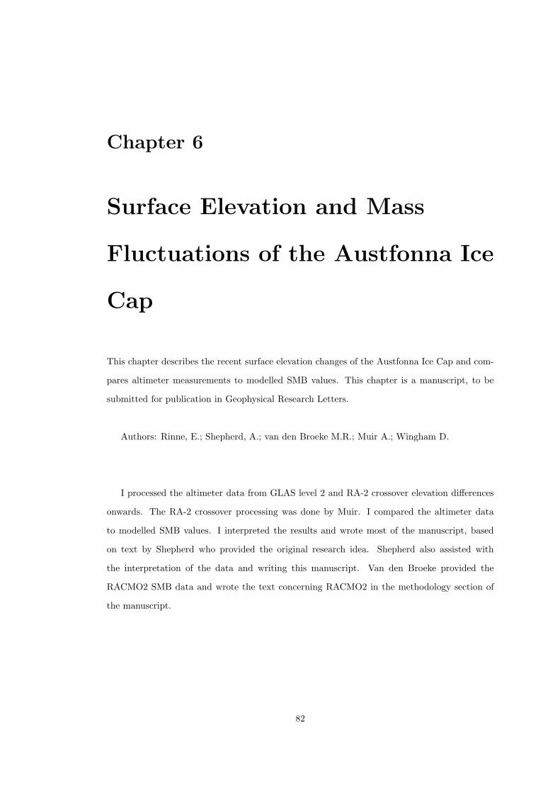
Chapter 6
Surface Elevation and Mass
Fluctuations of the Austfonna Ice
Cap
This chapter describes the recent surface elevation changes of the Austfonna Ice Cap and com-
pares altimeter measurements to modelled SMB values. This chapter is a manuscript, to be
submitted for publication in Geophysical Research Letters.
Authors: Rinne, E.; Shepherd, A.; van den Broeke M.R.; Muir A.; Wingham D.
I processed the altimeter data from GLAS level 2 and RA-2 crossover elevation differences
onwards. The RA-2 crossover processing was done by Muir. I compared the altimeter data
to modelled SMB values. I interpreted the results and wrote most of the manuscript, based
on text by Shepherd who provided the original research idea. Shepherd also assisted with
the interpretation of the data and writing this manuscript. Van den Broeke provided the
RACMO2 SMB data and wrote the text concerning RACMO2 in the methodology section of
the manuscript.
82
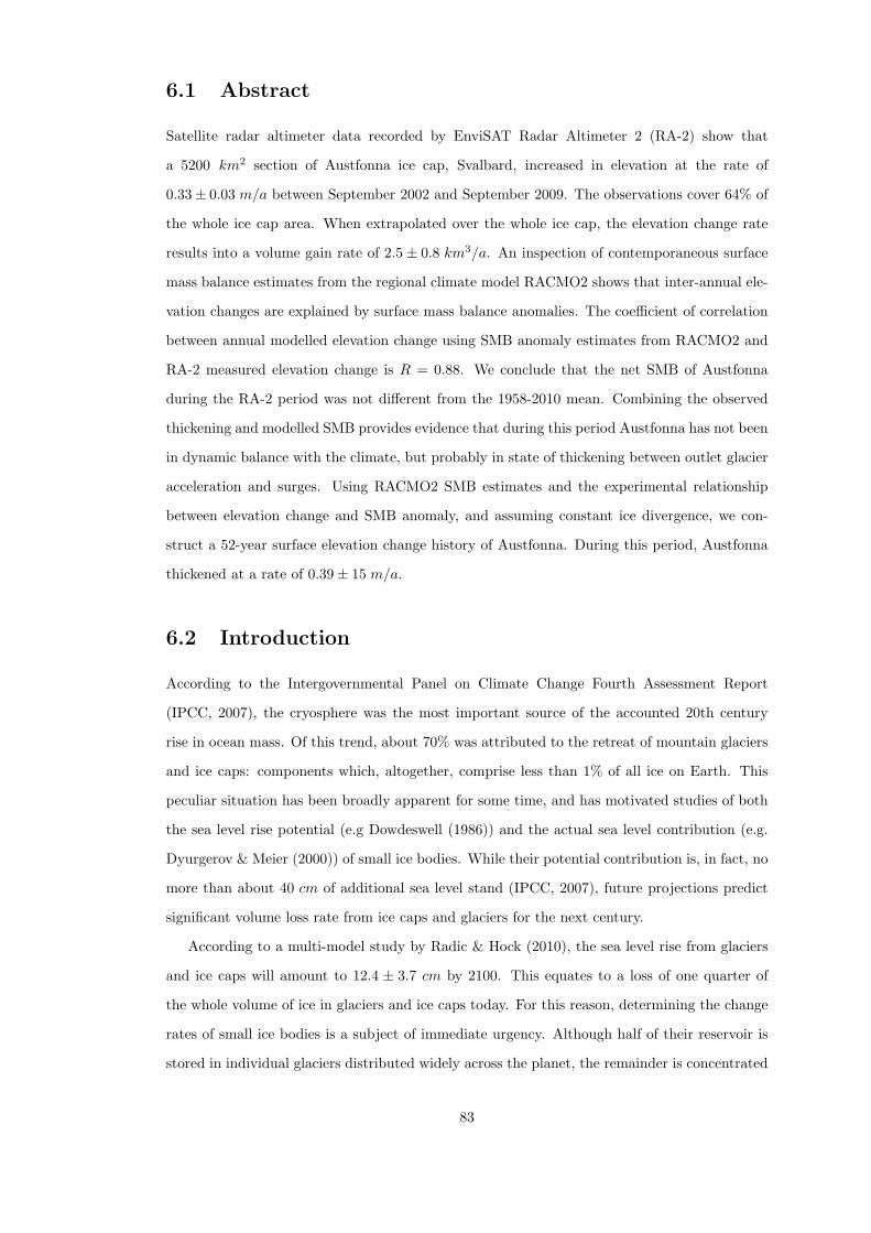
6.1 Abstract
Satellite radar altimeter data recorded by EnviSAT Radar Altimeter 2 (RA-2) show that
a 5200 km2 section of Austfonna ice cap, Svalbard, increased in elevation at the rate of
0.33± 0.03 m/a between September 2002 and September 2009. The observations cover 64% of
the whole ice cap area. When extrapolated over the whole ice cap, the elevation change rate
results into a volume gain rate of 2.5± 0.8 km3/a. An inspection of contemporaneous surface
mass balance estimates from the regional climate model RACMO2 shows that inter-annual ele-
vation changes are explained by surface mass balance anomalies. The coefficient of correlation
between annual modelled elevation change using SMB anomaly estimates from RACMO2 and
RA-2 measured elevation change is R = 0.88. We conclude that the net SMB of Austfonna
during the RA-2 period was not different from the 1958-2010 mean. Combining the observed
thickening and modelled SMB provides evidence that during this period Austfonna has not been
in dynamic balance with the climate, but probably in state of thickening between outlet glacier
acceleration and surges. Using RACMO2 SMB estimates and the experimental relationship
between elevation change and SMB anomaly, and assuming constant ice divergence, we con-
struct a 52-year surface elevation change history of Austfonna. During this period, Austfonna
thickened at a rate of 0.39± 15 m/a.
6.2 Introduction
According to the Intergovernmental Panel on Climate Change Fourth Assessment Report
(IPCC, 2007), the cryosphere was the most important source of the accounted 20th century
rise in ocean mass. Of this trend, about 70% was attributed to the retreat of mountain glaciers
and ice caps: components which, altogether, comprise less than 1% of all ice on Earth. This
peculiar situation has been broadly apparent for some time, and has motivated studies of both
the sea level rise potential (e.g Dowdeswell (1986)) and the actual sea level contribution (e.g.
Dyurgerov & Meier (2000)) of small ice bodies. While their potential contribution is, in fact, no
more than about 40 cm of additional sea level stand (IPCC, 2007), future projections predict
significant volume loss rate from ice caps and glaciers for the next century.
According to a multi-model study by Radic & Hock (2010), the sea level rise from glaciers
and ice caps will amount to 12.4 ± 3.7 cm by 2100. This equates to a loss of one quarter of
the whole volume of ice in glaciers and ice caps today. For this reason, determining the change
rates of small ice bodies is a subject of immediate urgency. Although half of their reservoir is
stored in individual glaciers distributed widely across the planet, the remainder is concentrated
83
in about 102 ice caps sited at polar latitudes. In consequence, establishing a mechanism to
determine fluctuations in the volume of ice caps with adequate accuracy offers an effective
means to reduce the present uncertainty in estimates of global sea level trend.
Austfonna is an ice cap covering 8120 km2 of Nordauslandet, the northernmost island of
the Svalbard archipelago. With a volume of 1900 km3 (Dowdeswell, 1986), corresponding to
0.75% of all ice beyond Antarctica and Greenland, Austfonna is the fourth largest ice cap on
Earth today (Dowdeswell & Hagen, 2004). According to accumulation studies by Pinglot et al.
(2001), Austfonna receives about 4 km3 w.e. of snow each year, or 0.25 % of its current mass.
Such a high level of turnover renders studies of the ice cap mass balance problematic, because
there is considerable natural variability at seasonal and inter-annual time scales. Nevertheless,
a number of studies have considered the mass balance of Austfonna.
According to an assessment of glaciological records collected during the late 20th century,
the estimated mass of Austfonna did not change significantly between 1963 and 1997 (Hagen
et al., 2003). However, a series of more recent, short-period surveys have reached markedly
different conclusions. Repeat aircraft laser altimeter measurements have shown that the central
accumulation area thickened by about 0.5 m/a between 1996 and 2002 (Bamber et al., 2004).
Bamber et al. (2004) and Raper et al. (2005) both labeled this thickening anomalous, attributing
it to an increasing precipitation trend associated with the decline of sea ice in the adjacent
Barents Sea. A survey of the ice cap mass budget during the 1990s, based on satellite-derived
velocities, detected a mass gain of 0.5 ± 0.2 Gt/a (Bevan et al., 2007). Finally, Moholdt et al.
(2010a) estimated the surface elevation changes of Austfonna using a combination of in-situ GPS
as well as airborne- and satellite altimetry. For the period of 2002-2008 they found an overall
mean elevation change rate of 0.05 ± 0.02 m/a and a total mass balance of −1.3 km3/a w.e.,
the majority of which they attributed to marine retreat loss.
In this work, we combine repeat measurements from the European Space Agency’s Environ-
mental Satellite (EnviSAT) radar altimeter (RA-2) and surface mass balance (SMB) estimates
from the Regional Atmospheric Climate Model (RACMO2). Our objective is to quantify the
volume change of Austfonna during the RA-2 period 2002-2009, and to characterize the origins
of the ice cap’s surface elevation fluctuations over the past five decades.
Even with spatial resolution coarser than that of laser altimeter, the RA-2 has been shown
to provide elevation change estimates of ice caps – targets previously considered to be too small
for radar altimeters. Importantly the RA-2 provides a longer time series and a better temporal
resolution than ICESat GLAS. Even if short time series of satellite altimeters does not allow
to determine long term surface elevation trends, combined with longer time series of modelled
84
SMB values it can improve our understanding of long term ice cap mass balance.
6.3 Data and Methods
We analysed elevation measurements from the EnviSAT RA-2 to determine the volume change
of the Austfonna ice cap between 2002 and 2009. To assess the elevation change rate from
RA-2, we employed the dual crossover method previously used to assess the elevation change
of the Antarctic Ice Sheet (Wingham et al., 1998), GrIS (Thomas et al., 2008), Flade Isblink
Ice Cap (Paul et al., 2011) and the Devon Ice Cap (Rinne et al., 2011). The method is based
on the dh/dt -method introduced by Zwally et al. (1989).
The Flade Isblink and Devon ice caps are targets of size and surface slopes similar to
Austfonna. The surface tracking system of the RA-2 is designed to be more robust than its
predecessors (Resti et al., 1999a). The autonomous resolution selection, part of the surface
tracking system, of the RA-2 has been shown to work on targets where previous altimeters
have failed (Legresy et al., 2005). To obtain ice surface elevation, the altimeter range mea-
surements were adjusted for perturbations in the satellite orbit and the effects of atmospheric
propagation delays. We did not apply any correction for co-varying changes in the elevation
and backscattered power observed elsewhere, because in regions of such high firn density the
degree of radar penetration is small (Shepherd et al., 2003). To quantify uncertainty introduced
by time-variant penetration, we compared the elevation change rates derived from late summer
(when the ice cap surface is expected to be wet and radar penetration is negligible) to elevation
change rates derived using all of the RA-2 measurements. The RMS difference of the two was
only 13 cm, which is smaller than our average trend uncertainty estimate. Furthermore, in the
RA-2 / RACMO2 comparison we used only data collected in August.
Our RA-2 method and its accuracy are discussed in detail by Rinne et al. (2011). To recap
briefly, the foundation of the method is to define the change in elevation over time in orbital
crossover points. Several of these elevation change measurements are combined into a time
series of relative elevation, and the elevation trend (and its 1-σ uncertainty) are determined by
linear regression.
The largest error sources contributing to the radar altimeter measurement are radar speckle
(associated with sub-footprint surface topography) and time-variant penetration of the radar
signal into the snow-pack (Arthern et al., 2001). These error sources are, in general, poorly
quantified. In the absence of formal estimates of error for RA-2 over ice caps, we use the 1-σ
confidence interval provided by the regression of the trend as our uncertainty estimate.
85
To assemble time series of elevation change, we used 10 different orbit repeat cycles as
references. In total we were able to form 51 separate time series of elevation change for 10x10 km
data bins, encompassing 64% of the Austfonna ice cap. From these data, we computed the
average elevation change rate at each data bin on the ice cap, elevation change rates for different
elevation bands, as well as the average elevation change rate of the whole ice cap.
To account for the elevation trend due to fluctuations in SMB, we examined monthly SMB
data from the RACMO2 at 11km horizontal resolution. Ettema et al. (2009) and Ettema et al.
(2010) showed that RACMO2 accurately simulates the present-day climate of the Greenland
Ice Sheet: present-day SMB correlates well with observations from snow pits and snow cores.
The atmospheric part of the model is forced at the lateral boundaries and the sea surface by the
interim-reanalysis of the European Centre for Medium-Range Weather Forecasts (ECMWF),
ERA-Interim for the years 1989-2009. For the period 1958-1988 ERA40 is used for forcing.
Although originally built for the Greenland Ice Sheet, RACMO2 also yields SMB estimates
for the Svalbard archipelago. The Austfonna ice cap lies close to the margin of RACMO2
domain and approximately 1000 km from the validation areas. Thus the RACMO2 SMB
values we use are not formally validated on Austfonna and they may include biases and other
errors. Our RACMO2 SMB estimates span a 52-year period 1958-2009. To allow comparison
of RA-2 observed elevation changes and RACMO2 SMB estimates, we calculated the annual
August to August elevation change for the RA-2. Since the first RA-2 data available are from
September 2002, the annual value for 2002-2003 is from September to August.
6.4 Results
The elevation change rate map of Austfonna measured by RA-2 is presented in Figure 6.1.
Our RA-2 measurements cover an area of 5100 km2 (64 % of the whole ice cap). Gaps in the
RA-2 data are usually due to “loss of lock” due to steep surface geometry. Missing data can
also be due to missing orbits or unsuccessful altimeter corrections. Between 2002 and 2009,
the section measured by RA-2 of the Austfonna ice cap gained elevation at the average rate
of 0.33 ± 0.08 m/a. The only area thinning according to our study is near the ice margin in
the south-east part of the ice cap. The negative rates at two data bins in the western part
of the ice cap are zero within the uncertainty. The area undergoing thinning is at one of the
few fast-flowing outlet glaciers of Austfonna. The map suggests an altitudinal pattern of the
elevation change rates: the largest thickening has taken place in the high elevation centre parts
of the ice cap.
86
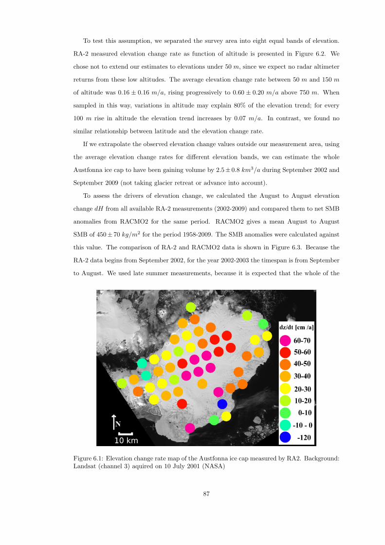
To test this assumption, we separated the survey area into eight equal bands of elevation.
RA-2 measured elevation change rate as function of altitude is presented in Figure 6.2. We
chose not to extend our estimates to elevations under 50 m, since we expect no radar altimeter
returns from these low altitudes. The average elevation change rate between 50 m and 150 m
of altitude was 0.16 ± 0.16 m/a, rising progressively to 0.60 ± 0.20 m/a above 750 m. When
sampled in this way, variations in altitude may explain 80% of the elevation trend; for every
100 m rise in altitude the elevation trend increases by 0.07 m/a. In contrast, we found no
similar relationship between latitude and the elevation change rate.
If we extrapolate the observed elevation change values outside our measurement area, using
the average elevation change rates for different elevation bands, we can estimate the whole
Austfonna ice cap to have been gaining volume by 2.5± 0.8 km3/a during September 2002 and
September 2009 (not taking glacier retreat or advance into account).
To assess the drivers of elevation change, we calculated the August to August elevation
change dH from all available RA-2 measurements (2002-2009) and compared them to net SMB
anomalies from RACMO2 for the same period. RACMO2 gives a mean August to August
SMB of 450± 70 kg/m2 for the period 1958-2009. The SMB anomalies were calculated against
this value. The comparison of RA-2 and RACMO2 data is shown in Figure 6.3. Because the
RA-2 data begins from September 2002, for the year 2002-2003 the timespan is from September
to August. We used late summer measurements, because it is expected that the whole of the
Figure 6.1: Elevation change rate map of the Austfonna ice cap measured by RA2. Background:Landsat (channel 3) aquired on 10 July 2001 (NASA)
87
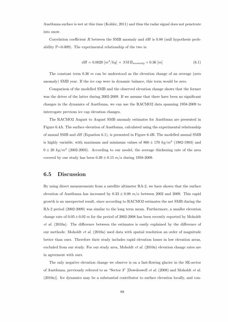
Austfonna surface is wet at this time (Kohler, 2011) and thus the radar signal does not penetrate
into snow.
Correlation coefficient R between the SMB anomaly and dH is 0.88 (null hypothesis prob-
ability P=0.009). The experimental relationship of the two is:
dH = 0.0020 [m3/kg] ∗ SMBanomaly + 0.36 [m] (6.1)
The constant term 0.36 m can be understood as the elevation change of an average (zero
anomaly) SMB year. If the ice cap were in dynamic balance, this term would be zero.
Comparison of the modelled SMB and the observed elevation change shows that the former
was the driver of the latter during 2002-2009. If we assume that there have been no significant
changes in the dynamics of Austfonna, we can use the RACMO2 data spanning 1958-2009 to
interrogate previous ice cap elevation changes.
The RACMO2 August to August SMB anomaly estimates for Austfonna are presented in
Figure 6.4A. The surface elevation of Austfonna, calculated using the experimental relationship
of annual SMB and dH (Equation 6.1), is presented in Figure 6.4B. The modelled annual SMB
is highly variable, with maximum and minimum values of 860 ± 170 kg/m2 (1982-1983) and
0 ± 20 kg/m2 (2002-2003). According to our model, the average thickening rate of the area
covered by our study has been 0.39± 0.15 m/a during 1958-2009.
6.5 Discussion
By using direct measurements from a satellite altimeter RA-2, we have shown that the surface
elevation of Austfonna has increased by 0.33 ± 0.08 m/a between 2002 and 2009. This rapid
growth is an unexpected result, since according to RACMO2 estimates the net SMB during the
RA-2 period (2002-2009) was similar to the long term mean. Furthermore, a smaller elevation
change rate of 0.05±0.02 m for the period of 2002-2008 has been recently reported by Moholdt
et al. (2010a). The difference between the estimates is easily explained by the difference of
our methods: Moholdt et al. (2010a) used data with spatial resolution an order of magnitude
better than ours. Therefore their study includes rapid elevation losses in low elevation areas,
excluded from our study. For our study area, Moholdt et al. (2010a) elevation change rates are
in agreement with ours.
The only negative elevation change we observe is on a fast-flowing glacier in the SE-sector
of Austfonna, previously referred to as “Sector 3” [Dowdeswell et al. (2008) and Moholdt et al.
(2010a)]. Ice dynamics may be a substantial contributor to surface elevation locally, and con-
88
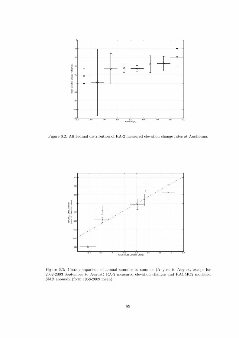
100 200 300 400 500 600 700 800 900−0.8
−0.6
−0.4
−0.2
0
0.2
0.4
0.6
0.8
1
Elevation [m]
Mea
n E
leva
tion
Cha
nge
Rat
e [m
/a]
Figure 6.2: Altitudinal distribution of RA-2 measured elevation change rates at Austfonna.
−0.4 −0.2 0 0.2 0.4 0.6 0.8 1 1.2
−500
−400
−300
−200
−100
0
100
200
300
RA2 Observed Elevation Change
RA
CM
O2
SM
B A
nom
aly
(kg/
m2 o
ff 19
58−
2010
mea
n)
Figure 6.3: Cross-comparison of annual summer to summer (August to August, except for2002-2003 September to August) RA-2 measured elevation changes and RACMO2 modelledSMB anomaly (from 1958-2009 mean).
89
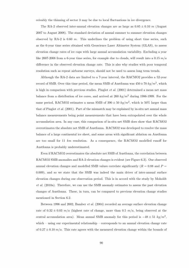
ceivably the thinning of sector 3 may be due to local fluctuations in ice divergence.
The RA-2 observed inter-annual elevation changes are as large as 0.85 ± 0.10 m (August
2007 to August 2008). The standard deviation of annual summer to summer elevation changes
observed by RA-2 is 0.60 m. This underlines the problem of using short time series, such
as the 6-year time series obtained with Geoscience Laser Altimeter System (GLAS), to assess
elevation change rates of ice caps with large annual accumulation variability. Excluding a year
like 2007-2008 from a 6-year time series, for example due to clouds, will result into a 0.15 m/a
difference in the observed elevation change rate. This is also why studies with poor temporal
resolution such as repeat airborne surveys, should not be used to assess long term trends.
Although the RA-2 data are limited to a 7-year interval, the RACMO2 provides a 52-year
record of SMB. Over this time period, the mean SMB of Austfonna was 450± 70 kg/m2, which
is high in comparison with previous studies. Pinglot et al. (2001) determined a mean net mass
balance from a distribution of ice cores, and arrived at 260 kg/m2 during 1986-1999. For the
same period, RACMO2 estimates a mean SMB of 390 ± 50 kg/m2, which is 50% larger than
that of Pinglot et al. (2001). Part of the mismatch may be explained by in-situ net annual mass
balance measurements being point measurements that have been extrapolated over the whole
accumulation area. In any case, this comparison of in-situ net SMB does show that RACMO2
overestimates the absolute net SMB of Austfonna. RACMO2 was developed to resolve the mass
balance of a large continental ice sheet, and some areas with significant ablation on Austfonna
are too small for 11 km resolution. As a consequence, the RACMO2 modelled runoff for
Austfonna is probably underestimated.
Even if RACMO2 overestimates the absolute net SMB of Austfonna, the correlation between
RACMO2 SMB anomalies and RA-2 elevation changes is evident (see Figure 6.3). Our observed
annual elevation changes and modelled SMB values correlate significantly (R = 0.88 and P =
0.009), and so we state that the SMB was indeed the main driver of inter-annual surface
elevation changes during our observation period. This is in accord with the study by Moholdt
et al. (2010a). Therefore, we can use the SMB anomaly estimates to assess the past elevation
changes of Austfonna. These, in turn, can be compared to previous elevation change studies
mentioned in Section 6.2.
Between 1996 and 2002, Bamber et al. (2004) recorded an average surface elevation change
rate of 0.32 ± 0.03 m/a (highest rate of change, more than 0.5 m/a, being observed at the
central accumulation area). Mean annual SMB anomaly for this period is −48 ± 51 kg/m2,
which – using our experimental relationship – corresponds to an annual elevation change rate
of 0.27± 0.10 m/a. This rate agrees with the measured elevation change within the bounds of
90
the experimental error. We conclude that the growth reported by Bamber et al. (2004) was not
anomalous but, in fact, similar to that of the long time mean.
As for the limitations of deriving surface elevation changes using RACMO2, we assume the
net effect of all of the factors contributing to elevation change not due to SMB to be constant
every year. In other words, we assume that the inter-annual variation of both firnification and
ice flow is negligible. As outlet glaciers surges have been reported in the past, the most recent
being the surge of Brasvellbreen in 1938 (Schytt, 1969), this assumption is not valid for long
term. However, several studies (e.g. Moholdt et al. (2010a) and Bevan et al. (2007)) have
concluded Austfonna to be in a quiescent phase of a surge cycle, and thus flow velocities are
both small and constant. Unfortunately, no studies of firn density fluctuations are available
for Arctic ice caps, and therefore we cannot quantitatively evaluate our assumption of constant
firnification rate.
6.6 Conclusions
1. The RA-2 observed elevation change rate of Ausfonna during 2002-2009 is 0.33 ± 0.08m/a,
resulting in volume gain of 2.6± 0.6 km3/a (not taking glacier retreat or advance into account)
when extrapolated over the whole ice cap surface. The RA-2 observed thickening provides
evidence that Austfonna is not in dynamic balance with the current climate, but probably in
state of thickening between outlet glacier surges.
2. The inter-annual variability of Austfonna’s surface elevation – and, in consequence,
volume – is driven by anomalies in surface mass balance.
3. For the first time, we have shown that satellite altimeter observations, combined with
SMB estimates from a regional climate model, can be used to assess past elevation changes
of an ice cap. Based on RACMO2 modelled SMB anomalies, we present an average elevation
change rate estimate of 0.39± 0.15 m/a for our study area during the period 1959-2009.
4. For the third time, the RA-2 has been used to succesfully survey the surface elevation
change of an ice cap. We establish that targets of this size are not too small for the resolution
attained by traditional radar altimeters.
5. Knowing that mass loss from ice caps is a significant contributor to present-day sea level
rise, an accurate estimate of its magnitude is an important goal of today’s cryospheric research.
Our technique offers a very real prospect of reducing the current uncertainty in the volume
change rate of ice caps.
91
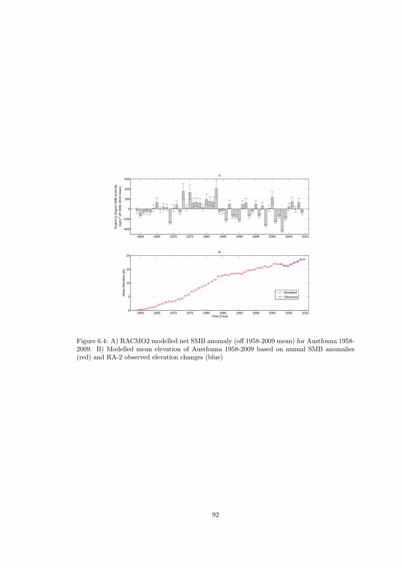
1960 1965 1970 1975 1980 1985 1990 1995 2000 2005 20100
5
10
15
20
Time [Year]
Mea
n E
leva
tion
[m]
B
1960 1965 1970 1975 1980 1985 1990 1995 2000 2005 2010
−400
−200
0
200
400
600
Aug
ust t
o A
ugus
t SM
B a
nom
aly
(kg/
m2 o
ff 19
58−
2010
mea
n)
A
ModelledObserved
Figure 6.4: A) RACMO2 modelled net SMB anomaly (off 1958-2009 mean) for Austfonna 1958-2009. B) Modelled mean elevation of Austfonna 1958-2009 based on annual SMB anomalies(red) and RA-2 observed elevation changes (blue)
92
Chapter 7
Discussion and Conclusions
This chapter summarises the findings of this thesis as presented in Chapters 4, 5 and 6 and
discusses their wider importance. The remaining challenges of altimeter ice cap elevation change
measurements are presented. Significance of the results are also discussed with respect to current
and future satellite missions.
7.1 Summary of Main Conclusions
The three main results chapters 4, 5 and 6 form a continuum of research work specifically demon-
strating the use of satellite altimetry for measuring surface elevation changes of ice caps. First,
in Chapter 4, the suitability of our technique is secured by cross-comparison of two independent
data sets on DIC. Next, the technique is applied to FIIC, and supported by independent SMB
estimates in Chapter 5. Finally, the satellite altimeter observations of current elevation change
of AIC are combined with a long time-series of SMB estimates, in order to assess past elevation
changes of the ice cap in Chapter 6.
7.1.1 Devon Ice Cap
The RA-2 and GLAS measured elevation changes on the DIC agree (RMS = 56 cm and
R = 0.68). GLAS has been previously used on ice caps, but this is the first study of a target
this size using a satellite radar altimeter like RA-2. The mean elevation change of the areas
of the DIC, that the RA-2 is able to measure, is zero within the uncertainty. Based on RA-2
measurements, the western arm of the DIC was thinning at a rate of 0.71± 0.49 m/a between
2002-2008. Furthermore, evidence of a localised 2 m drop in the surface elevation of the South
Croker Bay Glacier during summer 2007 was presented. This drop is apparent within both
93
satellite data sets, and was interpreted to reflect a speedup of the glacier.
7.1.2 Flade Isblink Ice Cap
The average surface elevation and mass change rates of the FIIC has been zero within the
uncertainty (0.03 ± 0.03 m/a and 0.0 ± 0.5 Gt/a, respectively) between September 2002 and
September 2009. However, the areas above late summer snow line were gaining elevation (on
average 0.09±0.04 m/a) and areas below it were losing elevation (on average −0.16±0.05 m/a)
between 2002 and 2009. The GLAS-observed local elevation change rates during 2004-2008
range from 3.4 ± 0.7 m/a to −2.5 ± 0.7 m/a. The maximum value is among the fastest
thickening reported anywhere in Greenland.
In the flat regions of the FIIC with only few slow and steady flowing outlet glaciers, the
annual surface elevation changes can be explained by annual variations in the net SMB. A
strong correlation (R = 0.97 and P = 0.0004) between the two is found. In the vicinity of
glaciers that have recently surged, net SMB does not explain the observed elevation changes,
and no correlation is found between the two (R = 0.38, P = 0.40).
7.1.3 Austfonna Ice Cap
The RA-2 observed elevation change rate of AIC was 0.33 ± 0.08m/a during 2002-2009. This
corresponds to a volume gain rate of 2.6 ± 0.6 km3/a (not taking glacier retreat or advance
into account) when extrapolated over the whole ice cap surface. The RA-2 observed thickening
provides evidence that AIC is not in dynamic balance with the current climate, but probably
in a state of thickening between outlet glacier surges.
During the observation period, the inter-annual variability of AIC’s surface elevation – and,
in consequence, volume – was driven by anomalies in SMB. Based on RACMO2 modelled SMB
anomalies, the average elevation change rate was estimated at 0.39±0.15 m/a during the period
1959-2009. Of the three ice caps studied, significant average changes were observed only on
AIC.
7.2 Remaining Challenges
A major remaining challenge in satellite altimeter remote sensing of ice caps is how to interpret
the trends derived from data measured during a relatively short limited time-span. Another
challenge, characteristic of radar altimeters, is the varying signal penetration to the snow pack,
which can introduce errors in the elevation change estimates. In addition, the RA-2 still suffers
94
from loss of tracking lock, and thus provides no measurements from the low elevation areas of
ice caps, with typically high surface slopes as well as high ablation rates. This is problematic,
because the largest elevation changes are expected to occur in these areas. However, a new
generation satellite altimeter flying with the CryoSat-2 is already able to measure areas with
high surface slopes (see Section 7.4.2)
As discussed in Section 1.1, in the context of climate change, the global sea level rise
contribution of the ice caps is of acute interest. Reliable quantification of this contribution calls
for more accurate and extensive snow and firn density estimates than are currently available.
7.2.1 Limited Time-span of Available Satellite Measurements
The currently available satellite altimeter data covers only a relatively short time-span. The
first ever satellite altimeter to measure land ice surface elevations was ALT onboard Seasat
in 1978 (see Section 2.6). GLAS data is only available for 2003-2009, and RA-2 data spans
from September 2002 to the present. It must be understood that the surface elevation change
rate measured by GLAS or RA-2 can not yet represent the long term trend. It is tempting
to make projections of the future change rates based on the GLAS or RA-2 data. However,
depending on the measurement period, the observed trend can be either negative or positive
(see for example Figure 4.4, the RA-2 measured relative elevations from the north-west sector
of the DIC).
Nevertheless, satellite altimeter data can – and should – be used when assessing different
theories and models discussing the drivers of the elevation changes, like was done in Chapters 5
and 6 where the annual elevation changes were shown to follow anomalies in SMB or, in other
areas, dynamic events. These theories can in turn be used when estimating past and future
elevation changes; In Section 6.4 the relationship between modelled SMB and observed elevation
change during the RA-2 period 2002-2009 was used to derive elevation change estimates during
1958-2002 from SMB values. In this manner, using satellite altimeter observations in tandem
with suitable models, like the RACMO2, they add to the knowledge of changes in ice caps even
outside the satellites’ lifetime.
7.2.2 Radar Penetration
As discussed in Chapters 4, 5 and 6, the variability of radar signal penetration into the target
surface introduces an uncertainty to RA-2 elevation change rate measurements. Penetration
corrections based on the backscattered power for radar altimeters do exist (Arthern et al., 2001),
and they have been utilised with RA measurements on continental ice sheets (e.g. Zwally et al.
95
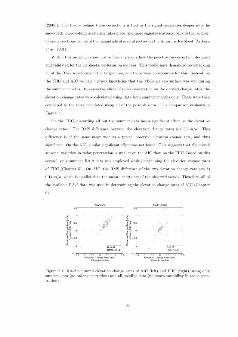
(2005)). The theory behind these corrections is that as the signal penetrates deeper into the
snow-pack, more volume scattering takes place, and more signal is scattered back to the receiver.
These corrections can be of the magnitude of several metres on the Antarctic Ice Sheet (Arthern
et al., 2001).
Within this project, I chose not to formally study how the penetration correction, designed
and validated for the ice sheets, performs on ice caps. This would have demanded re-retracking
all of the RA-2 waveforms in the target area, and there were no resources for this. Instead, on
the FIIC and AIC we had a priori knowledge that the whole ice cap surface was wet during
the summer months. To assess the effect of radar penetration on the derived change rates, the
elevation change rates were calculated using data from summer months only. These were then
compared to the rates calculated using all of the possible data. This comparison is shown in
Figure 7.1.
On the FIIC, discarding all but the summer data has a significant effect on the elevation
change rates. The RMS difference between the elevation change rates is 0.39 m/a. This
difference is of the same magnitude as a typical observed elevation change rate, and thus
significant. On the AIC, similar significant effect was not found. This suggests that the overall
seasonal variation in radar penetration is smaller on the AIC than on the FIIC. Based on this
control, only summer RA-2 data was employed while determining the elevation change rates
of FIIC (Chapter 5). On AIC, the RMS difference of the two elevation change rate sets is
0.14 m/a, which is smaller than the mean uncertainty of the observed trends. Therefore, all of
the available RA-2 data was used in determining the elevation change rates of AIC (Chapter
6).
−1.5 −1 −0.5 0 0.5 1 1.5−1.5
−1
−0.5
0
0.5
1
1.5
Elevation Change Rate [m/a] All available data
Ele
vatio
n C
hang
e R
ate
[m/a
] S
umm
er d
ata
only
Austfonna
−1.5 −1 −0.5 0 0.5 1 1.5−1.5
−1
−0.5
0
0.5
1
1.5
Elevation Change Rate [m/a] All available data
Ele
vatio
n C
hang
e R
ate
[m/a
] S
umm
er d
ata
only
Flade Isblink
R=0.51RMS = 0.39
R=0.91RMS = 0.14
Figure 7.1: RA-2 measured elevation change rates of AIC (left) and FIIC (right), using onlysummer data (no radar penetration) and all possible data (unknown variability in radar pene-tration)
96
On the DIC (Chapter 4), RA-2 measurements without penetration correction were utilised.
The variation of radar penetration was accepted as one of the factors contributing to the
mismatch of GLAS and RA-2 elevation change measurements. The agreement of the GLAS
and RA-2 measurements is still reasonable (Section 4.4.1) – suggesting that the variability of
radar penetration on the DIC is relatively small.
Even with the existing penetration corrections applied, Thomas et al. (2008) presented
possible errors in the elevation change estimates of the Greenland Ice Sheet derived from radar
altimeter measurements. These possible errors are caused by the radar penetration progressively
becoming smaller as the increasing temperatures affect the surface snow characteristics (seasonal
melt extent increases). If there are similar progressive changes in the seasonal melt extent on
an ice cap, similar errors might be present in ice cap surface elevation change rate estimates
derived from RA-2 data. On ice caps such as AIC and FIIC this not an issue, because melt
extends over the whole ice cap area even during a typical summer.
Overall, the feasibility of existing penetration range corrections to ice caps should be fur-
ther validated in the realm of ice caps. If found to perform well, these corrections should be
implemented in the future versions of RA-2 ice cap elevation change rate processors. Further-
more, ground-based radar studies similar to that of Scott et al. (2006) would be useful when
quantifying the penetration depths of radar signals to ice caps. Several campaigns would be
needed to quantify the variation of the radar penetration. In the meantime, the effect of us-
ing only summer data should be quantified before interpreting the change rates. If the use of
summer data only leads into markedly different results than the use of all-year data, variation
in penetration depth is probably present. In such cases, only the summer data should be used,
given that the whole ice cap surface is known to be wet during summer.
7.2.3 Contribution of Ice Caps to the Global Sea Level Rise
The main goal of this study, as stated in Section 1.2, was to add to the knowledge of the state
and change of the ice caps today. In case of surface elevation and volume changes, this goal
was reached. For DIC and AIC, no mass change estimates were derived. However, to assess
the contribution of ice caps to the global sea level rise, volume changes must be converted
into mass changes. For this, an estimate of ice cap density is required. If one has no a priori
knowledge of the density, the estimates will necessarily have large uncertainties that translate
into large uncertainties in the net mass change estimates. In Section 5.4, this uncertainty in
the firn density (660± 250 kg/m3) is accepted. In other words, it is accepted that the density
of the firn can be anything between that of typical first year snow (410 kg/m3) and pure ice
97
(910 kg/m3). Using this estimate, a FIIC mass change rate estimate of 0.0 ± 0.5 Gt/a was
derived. This zero mass change, naturally, corresponds to zero (0.000 ± 0.001 mm/a) change
in global sea level.
The same firn density estimate with the large uncertainty (660 ± 250kg/m3) was used by
Gardner et al. (2011) to convert GLAS measured surface elevation changes of Canadian ice
caps (including DIC) to mass changes. In addition to altimeter measurements, they also used
modelled mass balance and gravimetry and arrived at a total mass loss of 368 ± 41 Gt(or
1.01 ± 0.11 mm of sea-level rise) from the Canadian ice caps between the years 2004 to 2009.
Because 85% of the volume losses observed by Gardner et al. (2011) occurred below the firn
area, the large uncertainty in firn density had relatively small impact (±2Gt) on overall mass
loss estimates. This was not the case with the FIIC, where significant volume gain was observed
in the firn area (area above the LSSL) and the large uncertainty in firn density resulted in large
uncertainty in the mass change estimate.
For the large ice sheets, firn densities are derived from temperature-dependent snow models,
which have been shown to yield good results (e.g. Zwally et al. (2005) and Arthern et al. (2010)).
If the surface elevation changes derived from altimetry are to be converted to mass changes,
similar models must be validated at ice caps. Before that, the large uncertainty in the firn
density has to be accepted.
7.3 Future work
This thesis covers but three of the several hundreds of ice caps on Earth. The most important
outcome of the thesis lies in the demonstration that ice caps are feasible targets for traditional
radar altimetry. As a part of this project, 189 GlobGlacier WP4 (elevation change) products
have been created. More importantly, the processing software for RA-2 and GLAS data were
written and are available for further development.
The next logical step would be to use this software and extend a similar study across a large
number of ice caps. This would yield mean surface elevation (and volume) change estimates
for the target ice caps. Combined with validated density estimates from a suitable model, the
volume change estimates can be converted to mass change estimates.
The surface elevation change of an ice cap is mainly driven by the SMB and the dynamics
of the ice cap, but often it is unclear which one is the primary driver. If one has information on
the SMB (estimate of the long term mean from ice cores, fine resolution climate model, etc.)
drivers of the surface elevation can be assessed. A good example of this is our study on the
98
South Croker Bay Glacier on the DIC (Section 4.4.5). Two independent altimeters measured
a surface drop of approximately 2 m, that could not be explained by melt. It is likely that the
drop is due to ice dynamics, and the South Croker Bay Glacier would provide an interesting
target for future study. In case the of FIIC, the SMB estimates from RACMO2 were used to
assess the relationship of SMB and surface elevation change. Areas where SMB alone is the
driver of the elevation change, as well as areas where it is not, could be distinguished from each
other by quantitative means. As discussed in Section 1.3.1, there is a need for a geographically
extensive study on relative importance of the SMB and dynamic effects. The work on the FIIC
presented in Chapter 5 of this thesis can be considered as a pilot study for such a geographically
extensive study.
The ability to observe whether a part of an ice cap is experiencing rapid dynamic effects,
would provide valuable information for the glaciological community. Searching for significant
thinning or thickening in all of the available RA-2 elevation time series would be reasonably easy
to automate. This, combined with an estimate for SMB of the area, and a simple threshold filter
(for example dh > 2∗SMB), could reveal surge-like behaviour and pinpoint areas of interest. A
more detailed study of velocity change could then be undertaken using InSAR derived surface
velocities. If ice caps with widespread dynamic thinning due to accelerated glacier flow would
be found, the trigger of this acceleration could be further studied. This, in turn, would result
in better estimates what magnitude of changes in boundary conditions of an ice cap would be
needed to trigger large scale dynamic mass losses that would result into sharp increase in the
rate of the global sea level rise.
7.4 Current and Future Satellite Altimeters
At the time of writing, there are two satellite altimeters suitable for remote sensing of land
ice in orbit: RA-2 and SIRAL-2. Two more satellite altimeters, that will provide altimeter
measurements similar to those discussed in this thesis, are planned: ATLAS and SRAL.
7.4.1 Radar Altimeter 2 During EnviSAT extension
In late 2010, the orbit of EnviSAT was changed to save the remaining hydrazine fuel on-board
the satellite. The change allows extension of the mission until the end of 2013, exceeding the
5-year nominal lifetime of the satellite by nearly 7 years (ESA Earthnet, 2010). Currently RA-2
is measuring surface elevations from the extension orbit.
As the RA-2 method described in this thesis relies on orbital crossover points, the orbit
99
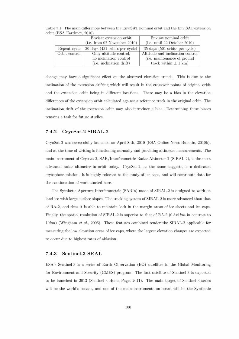
Table 7.1: The main differences between the EnviSAT nominal orbit and the EnviSAT extensionorbit (ESA Earthnet, 2010)
Envisat extension orbit Envisat nominal orbit(i.e. from 02 November 2010) (i.e. until 22 October 2010)
Repeat cycle 30 days (431 orbits per cycle) 35 days (501 orbits per cycle)Orbit control Only altitude control, Altitude and inclination control
no inclination control (i.e. maintenance of ground(i.e. inclination drift) track within ± 1 km)
change may have a significant effect on the observed elevation trends. This is due to the
inclination of the extension drifting which will result in the crossover points of original orbit
and the extension orbit being in different locations. There may be a bias in the elevation
differences of the extension orbit calculated against a reference track in the original orbit. The
inclination drift of the extension orbit may also introduce a bias. Determining these biases
remains a task for future studies.
7.4.2 CryoSat-2 SIRAL-2
CryoSat-2 was successfully launched on April 8:th, 2010 (ESA Online News Bulletin, 2010b),
and at the time of writing is functioning normally and providing altimeter measurements. The
main instrument of Cryosat-2, SAR/Interferometric Radar Altimeter 2 (SIRAL-2), is the most
advanced radar altimeter in orbit today. CryoSat-2, as the name suggests, is a dedicated
cryosphere mission. It is highly relevant to the study of ice caps, and will contribute data for
the continuation of work started here.
The Synthetic Aperture Interferometric (SARIn) mode of SIRAL-2 is designed to work on
land ice with large surface slopes. The tracking system of SIRAL-2 is more advanced than that
of RA-2, and thus it is able to maintain lock in the margin areas of ice sheets and ice caps.
Finally, the spatial resolution of SIRAL-2 is superior to that of RA-2 (0.3x1km in contrast to
10km) (Wingham et al., 2006). These features combined render the SIRAL-2 applicable for
measuring the low elevation areas of ice caps, where the largest elevation changes are expected
to occur due to highest rates of ablation.
7.4.3 Sentinel-3 SRAL
ESA’s Sentinel-3 is a series of Earth Observation (EO) satellites in the Global Monitoring
for Environment and Security (GMES) program. The first satellite of Sentinel-3 is expected
to be launched in 2013 (Sentinel-3 Home Page, 2011). The main target of Sentinel-3 series
will be the world’s oceans, and one of the main instruments on-board will be the Synthetic
100
Aperture Radar Altimeter (SRAL). SRAL will be a dual frequency (Ku and C-band) radio
altimeter, capable of synthetic aperture measurements for improved spatial resolution, much
like CryoSat-2’s SIRAL-2. However SRAL will lack the SARIn mode that would be most useful
for studying ice caps.
Sentinel-3 will provide operational observations for a multitude of applications, some of
which are time-critical. Thus some Sentinel-3 products will be available to users only hours
after the measurement, in contrast to the considerably longer processing times of data from
science satellites. ESA has also declared that the data from the Sentinel missions, including
the SRAL data, will be free (ESA Online News Bulletin, 2009).
Sentinel-3 satellites will fly in a high-inclination (98.5o), sun-synchronous polar orbits, so
they will provide potentially valuable altimeter measurements on polar land ice (Aguirre et al.,
2007). Even while lacking the SARIn mode, SRAL will provide data much like that of RA-
2. The work on RA-2 presented in this thesis is directly applicable to SRAL, even if the
measurements on ice caps would be made in a low resolution mode. If the EnviSAT can provide
RA-2 data until the end of the planned extension phase, SRAL will continue the time series of
elevation measurements with at least some overlap. When SRAL data becomes available, there
is no reason why it could not be utilised in ice cap elevation change studies.
7.4.4 ICESat-2 ATLAS
The Ice, Cloud, and land Elevation Satellite-2 (ICESat-2), scheduled for launch in 2016 (ICESat-
2 WWW page, 2011), is the follow-up of the ICESat mission. The main payload of the ICESat-2
will be the Advanced Topographic Laser Altimeter System (ATLAS). ATLAS will be a multi-
beam laser system loosely based on the GLAS, but with two major differences. Instead of a
single laser beam, ATLAS will have six beams in a 3x2 configuration (see Figure 7.2). Additional
measurements from both sides of the ground track will provide an estimate of cross-surface slope
– a source of uncertainty in GLAS measurements, discussed in Section 3.2.2. ATLAS will also
have a lower transmit energy and higher pulse repetition rate (PRF) than GLAS. This design
is known as the micropulse laser altimetry approach. High PRF will result in dense along-track
sampling. The proposed PRF for ATLAS is 10 kHz, resulting in along-track spacing of less
than one metre (Yu et al., 2010), in contrast to the 170 m spacing of GLAS.
ICESat-2, if successful, will provide data suitable for ice cap surface elevation change studies.
Combining ATLAS data with GLAS measurements will provide elevation change estimates for
the 13 year period between start of the GLAS measurements (2003) and the ATLAS measure-
ments (2016 onwards). Unfortunately, the mission is still in phase A, at least half of a decade
101
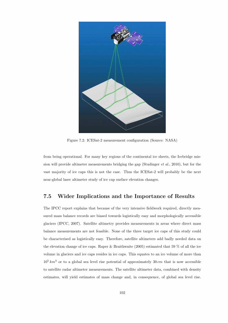
Figure 7.2: ICESat-2 measurement configuration (Source: NASA)
from being operational. For many key regions of the continental ice sheets, the Icebridge mis-
sion will provide altimeter measurements bridging the gap (Studinger et al., 2010), but for the
vast majority of ice caps this is not the case. Thus the ICESat-2 will probably be the next
near-global laser altimeter study of ice cap surface elevation changes.
7.5 Wider Implications and the Importance of Results
The IPCC report explains that because of the very intensive fieldwork required, directly mea-
sured mass balance records are biased towards logistically easy and morphologically accessible
glaciers (IPCC, 2007). Satellite altimetry provides measurements in areas where direct mass
balance measurements are not feasible. None of the three target ice caps of this study could
be characterised as logistically easy. Therefore, satellite altimeters add badly needed data on
the elevation change of ice caps. Raper & Braithwaite (2005) estimated that 59 % of all the ice
volume in glaciers and ice caps resides in ice caps. This equates to an ice volume of more than
105 km3 or to a global sea level rise potential of approximately 30 cm that is now accessible
to satellite radar altimeter measurements. The satellite altimeter data, combined with density
estimates, will yield estimates of mass change and, in consequence, of global sea level rise.
102
The accuracy of the mass change estimate is largely subject to the uncertainty of the density
estimate like discussed in Section 7.2.3.
Work presented in this thesis shows that the RA-2 data are valuable in measuring ice cap
surface elevation change. Previously this has been uncertain, and subject to debate. The
accumulation rates of Greenland, measured by satellite radar altimeters, were questioned in the
late 1990’s because “radar altimeter data are subject to large errors” (Benn & Evans, 1998).
Altimetry has since developed into a recognised tool for cryospheric research (see Sections 3.3
and 3.4). The work presented in this thesis is a continuation of this development, pushing the
size limit of the target smaller, and the resolution of elevation change rate maps finer. This
development can be seen by comparing Figures 3.6 (RA elevation change rate map of Greenland,
spatial resolution 100 km) and 5.3 (RA-2 elevation change rate map of FIIC, spatial resolution
10 km).
The demonstration of the feasibility of traditional radar altimetry for measuring ice cap ele-
vation changes is an important result. Laser altimeters have been previously used in measuring
ice cap elevation changes, and the GLAS data is widely accepted to be good (e.g. Moholdt et al.
(2010b), Gardner et al. (2011)) but at the time of writing there are no laser altimeters in orbit.
However, the RA-2 is still flying, and the results presented in this thesis show that it is able to
measure similar targets as GLAS, especially the large, flat ice caps. Thus we can continue to
monitor these ice caps with the RA-2, as well as the radar altimeters on-board future Sentinel-3
satellites.
The processors for RA-2 and GLAS data, written as part of this research project, now
form a part of the GlobGlacier system for monitoring glacier and ice caps changes from space.
Consequently, the work presented in this thesis will continue to contribute to ESA altimeter
data processing in the future.
7.6 Concluding Remarks
The work in this thesis shows that a traditional radar altimeter (namely the RA-2) can measure
elevation changes of ice caps. The elevation change estimates from RA-2 and GLAS are in
agreement, thus validating the RA-2 estimates. When radar altimetry had been previously
used on large ice sheets, the feasibility of RA-2 to measure ice caps was uncertain and subject
to debate prior to this work. The results of this thesis are a continuation of the development
of satellite remote sensing of the cryosphere. As an outcome of my work, elevation change
estimates of areas previously unmeasured can be obtained.
103

I have presented elevation change estimates, derived from both GLAS and RA-2, for ice
cap areas where no previous elevation change estimates existed. I have also shown that these
estimates, used in conjunction with modelled SMB estimates, can shed light on the drivers
of the elevation change. Given the importance of ice caps to the global sea level rise, this
knowledge will result in better quantification and understanding of the ongoing effects of global
climate change.
104
Bibliography
Abdalati, W., Krabill, W., Frederick, E., Manizade, S., Martin, C., Sonntag, J.,
Swift, R., Thomas, R., Yungel, J., & Koerner, R. 2004. Elevation changes of ice caps
in the Canadian Arctic Archipelago. JOURNAL OF GEOPHYSICAL RESEARCH-EARTH
SURFACE, 109(F4).
Aguirre, M., Berruti, B. Bezy, J-L., Drinkwater, M., Heliere, F., Klein, U., C.,
Mavrocordatos, & P., Silvestrin. 2007 (AUG). Sentinel-3 The Ocean and Medium-
Resolution Land Mission for GMES Operational Services. ESA Bulletin. ESTEC.
Arendt, A., Echelmeyer, K., Harrison, W., Lingle, C., Zirnheld, S., Valentine,
V., Ritchie, B., & Druckenmiller, M. 2006. Updated estimates of glacier volume
changes in the western Chugach Mountains, Alaska, and a comparison of regional extrapola-
tion methods. JOURNAL OF GEOPHYSICAL RESEARCH-EARTH SURFACE, 111(F3).
Arthern, RJ., Wingham, DJ., & Ridout, AL. 2001. Controls on ERS altimeter measure-
ments over ice sheets: Footprint-scale topography, backscatter fluctuations, and the depen-
dence of microwave penetration depth on satellite orientation. JOURNAL OF GEOPHYSI-
CAL RESEARCH-ATMOSPHERES, 106(D24), 33471–33484.
Arthern, RJ., Vaughan, DG., Rankin, AM., Mulvaney, R., & Thomas, ER. 2010.
In situ measurements of Antarctic snow compaction compared with predictions of models.
JOURNAL OF GEOPHYSICAL RESEARCH-EARTH SURFACE, 115(JUL 29).
Bamber, J., Krabill, W., Raper, V., & Dowdeswell, J. 2004. Anomalous recent growth
of part of a large Arctic ice cap: Austfonna, Svalbard. GEOPHYSICAL RESEARCH LET-
TERS, 31(12).
Bamber, JL. 1994. Ice-Sheet Altimeter Processing Scheme. INTERNATIONAL JOURNAL
OF REMOTE SENSING, 15(4), 925–938.
105
Bannoura, WJ., Wade, A., & Srinivas, DN. 2005. NOAA Ocean Surface Topography
Mission Jason-2 project overview. Pages 2155–2159 of: OCEANS 2005, VOLS 1-3. IEEE.
Bargellini, P., Garcia Matatoros, MA., Ventimiglia, L., & Suen, D. 2006. Envisat
attitude and orbit control in-orbit performance: An operational view. In: 6th International
ESA Conference on Guidance, Navigation and Control Systems, held 17-20 October 2005 in
Loutraki, Greece. ESA SP-606.
Benn, DI., & Evans, DJA. 1998. Glaciers & glaciation. Arnold Publishing.
Benveniste, J, Roca, M, Levrini, G, Vincent, P, Baker, S, Zanife, O, Zelli, C, &
Bonbaci, O. 2008 (NOV 9). The Radar Altimetry Mission: RA-2, MWR, DORIS and LRR.
ESA Bulletin. ESRIN.
Bevan, S., Luckman, A., Murray, T., Sykes, H., & Kohler, J. 2007. Positive mass
balance during the late 20th century on Austfonna, Svalbard, revealed using satellite radar
interferometry. Pages 117–122 of: ANNALS OF GLACIOLOGY, vol. 46. IGS.
Bougamont, M., & Bamber, JL. 2005. A surface mass balance model for the Greenland ice
sheet. JOURNAL OF GEOPHYSICAL RESEARCH-EARTH SURFACE, 110(F4).
Brandt, O., Bjornsson, H., & Gjessing, Y. 2005. Mass-balance rates derived by mapping
internal tephra layers in Myrdalsjokull and Vatnajokull ice caps, Iceland. ANNALS OF
GLACIOLOGY, vol. 42. IGS.
Brenner, AC., Zwally, HJ., Bentley, CR., Csatho, BM., Harding, DJ., Hofton,
MA., Minster, J-B., Roberts, LA., Saba, JL., Thomas, RH., & Yi, D. 2003 (Septem-
ber). Geoscience Laser Altimeter System (GLAS) Algorithm Theoretical Basis Document.
Derivation of Range and Range Distributions From Laser Pulse Waveform Analysis for Sur-
face Elevations, Roughness, Slope, and Vegetation Heights. Version 4.1.
Brenner, AC., DiMarzio, JP., & Zwally, HJ. 2007. Precision and accuracy of satellite
radar and laser altimeter data over the continental ice sheets. IEEE TRANSACTIONS ON
GEOSCIENCE AND REMOTE SENSING, 45(2), 321 –331.
Brooks, RL., Campbell, WJ., Ramseier, RO., Stanley, HR., & Zwally, HJ. 1978.
Ice Sheet Topography by Satellite Altimetry. NATURE, 274(5671), 539–543.
Burgess, D., & Sharp, M. 2008. Recent changes in thickness of the Devon Island ice cap,
Canada. JOURNAL OF GEOPHYSICAL RESEARCH-SOLID EARTH, 113(B7).
106
Burgess, DO., & Sharp, MJ. 2004. Recent changes in areal extent of the Devon Ice Cap,
Nunavut, Canada. ARCTIC ANTARCTIC AND ALPINE RESEARCH, 36(2), 261–271.
Cartwright, DE., & Edden, AC. 1973. Corrected tables of tidal harmonics. Geophysical
journal of the royal astronomical society, 33(3), 253–264.
Cole, TD., Maurer, R., & Kinnison, J. 2001. Performance of the NEAR laser altimeter
at the asteroid, 433 Eros, after 5 years in space. Pages 21–30 of: Berghmans, F and
Taylor, EW (ed), PHOTONICS FOR SPACE AND RADIATION ENVIRONMENTS II.
PROCEEDINGS OF THE SOCIETY OF PHOTO-OPTICAL INSTRUMENTATION EN-
GINEERS (SPIE), vol. 4547. 2nd Conference on Photonics for Space and Radiation Envi-
ronments, TOULOUSE, FRANCE, SEP 17-18, 2001.
Colgan, W., & Sharp, M. 2008. Combined oceanic and atmospheric influences on net
accumulation on Devon ice cap, nunavut, Canada. JOURNAL OF GLACIOLOGY, 54(184),
28–40.
Colgan, W., Davis, J., & Sharp, M. 2008. Is the high-elevation region of Devon Ice Cap
thickening? JOURNAL OF GLACIOLOGY, 54(186), 428–436.
Copland, L., Sharp, MJ., & Dowdeswell, JA. 2003. The distribution and flow charac-
teristics of surge-type glaciers in the Canadian High Arctic. ANNALS OF GLACIOLOGY,
vol. 36. IGS.
Davis, CH., & Ferguson, AC. 2004. Elevation change of the Antarctic ice sheet, 1995-2000,
from ERS-2 satellite radar altimetry. IEEE TRANSACTIONS ON GEOSCIENCE AND
REMOTE SENSING, 42(11), 2437–2445.
Davis, CH., Belu, RG., & Feng, G. 2001. Elevation change measurement of the East
Antarctic Ice Sheet, 1978 to 1988, from satellite radar altimetry. IEEE TRANSACTIONS
ON GEOSCIENCE AND REMOTE SENSING, 39(3), 635–644.
Davis, CH., Li, YH., McConnell, JR., Frey, MM., & Hanna, E. 2005. Snowfall-driven
growth in East Antarctic ice sheet mitigates recent sea-level rise. SCIENCE, 308(5730),
1898–1901.
Dowdeswell, JA. 1986. Drainage-Basin Characteristics Of Nordaustlandet Ice Caps, Sval-
bard. JOURNAL OF GLACIOLOGY, 32(110), 31–38.
Dowdeswell, JA. 2006. Atmospheric science - The Greenland Ice Sheet and global sea-level
rise. SCIENCE, 311(5763), 963–964.
107
Dowdeswell, JA., & Hagen, JO. 2004. Mass balance of the cryosphere. Cambridge Uni-
versity Press. Pages 527–557.
Dowdeswell, JA., Unwin, B., Nuttall, AM., & Wingham, DJ. 1999. Velocity structure,
flow instability and mass flux on a large Arctic ice cap from satellite radar interferometry.
EARTH AND PLANETARY SCIENCE LETTERS, 167(3-4), 131–140.
Dowdeswell, JA., Benham, TJ., Gorman, MR., Burgess, D., & Sharp, MJ. 2004.
Form and flow of the Devon Island Ice Cap, Canadian Arctic. JOURNAL OF GEOPHYSI-
CAL RESEARCH-EARTH SURFACE, 109(F2).
Dowdeswell, JA., Benham, TJ., Strozzi, T., & Hagen, JO. 2008. Iceberg calving flux
and mass balance of the Austfonna ice cap on Nordaustlandet, Svalbard. JOURNAL OF
GEOPHYSICAL RESEARCH-EARTH SURFACE, 113(F3).
Duda, DP., Spinhirne, JD., & Eloranta, EW. 2001. Atmospheric multiple scattering
effects on glas altimetry. i. calculations of single pulse bias. IEEE TRANSACTIONS ON
GEOSCIENCE AND REMOTE SENSING, 39(1), 92 –101.
Dyurgerov, MB., & Meier, MF. 2000. Twentieth century climate change: Evidence from
small glaciers. PROCEEDINGS OF THE NATIONAL ACADEMY OF SCIENCES OF THE
UNITED STATES OF AMERICA, 97(4), 1406–1411.
Eiken, T., Hagen, JO., & Melvold, K. 1997. Kinematic GPS survey of geometry changes
on Svalbard glaciers. ANNALS OF GLACIOLOGY, vol. 24. IGS.
ERS User Handbook. 1993. ERS User Handbook (ESA Publication SP-1148).
ESA Earthnet. 2010. Implementation of Envisat extension orbit in October 2010
(http://earth.esa.int/object/index.cfm?fobjectid=6999).
ESA Online News Bulletin. 2008 (Jan). ENVISAT RA-2 S-band anomaly 23 January 2008
(http://earth.esa.int/object/index.cfm?fobjectid=5483).
ESA Online News Bulletin. 2009 (Nov). ESA Member States approve full and open Sentinel
data policy principle, (http://www.esa.int/esaEO/SEMXK570A2G environment 0.html).
ESA Online News Bulletin. 2010a (Dec). ENVISAT Altimetry RA2 Data
(http://earth.esa.int/object/index.cfm?fobjectid=7363).
ESA Online News Bulletin. 2010b (Apr). Successful Launch for ESAs CryoSat-2 Ice Satel-
lite (http://www.esa.int/SPECIALS/Cryosat/SEMH5ZZNK7G 0.html).
108
Ettema, J., van den Broeke, MR., van Meijgaard, E., van de Berg, WJ., Bamber,
JL., Box, JE., & Bales, RC. 2009. Higher surface mass balance of the Greenland ice sheet
revealed by high-resolution climate modeling. GEOPHYSICAL RESEARCH LETTERS,
36(JUN 16).
Ettema, J., van den Broeke, M., van Meijgaard, E., van de Berg, WJ., JE., Box,
& Steffen, K. 2010. Climate of the Greenland ice sheet using a high-resolution climate
model Part 1: Evaluation. The cryosphere, 4, 561–602.
Fricker, HA., Borsa, A., Minster, B., Carabajal, C., Quinn, K., & Bills, B. 2005.
Assessment of ICESat performance at the Salar de Uyuni, Bolivia. GEOPHYSICAL RE-
SEARCH LETTERS, 32(21).
Fu, LL., Christensen, EJ., Yamarone, CA., Lefebvre, M., Menard, Y., Dorrer,
M., & Escudier, P. 1994. TOPEX/POSEIDON MISSION OVERVIEW. JOURNAL OF
GEOPHYSICAL RESEARCH-OCEANS, 99(C12), 24369–24381.
Gardner, AS., Sharp, MJ., Koerner, RM., Labine, C., Boon, S., Marshall, SJ.,
Burgess, DO., & Lewis, D. 2009. Near-Surface Temperature Lapse Rates over Arctic
Glaciers and Their Implications for Temperature Downscaling. JOURNAL OF CLIMATE,
22(16), 4281–4298.
Gardner, AS., Moholdt, G., Wouters, B., Wolken, GJ., Burgess, DO., Sharp,
MJ., Cogley, JG., Braun, C., & Labine, C. 2011. Sharply increased mass loss from
glaciers and ice caps in the Canadian Arctic Archipelago. NATURE.
Garvin, J., Bufton, J., Blair, J., Harding, D., Luthcke, S., Frawley, J., & Row-
lands, D. 1998. Observations of the earth’s topography from the shuttle laser altime-
ter (sla): Laser-pulse echo-recovery measurements of terrestrial surfaces. PHYSICS AND
CHEMISTRY OF THE EARTH, 23(9-10), 1053 – 1068.
Glickman, TS. 2000. Glossary of meteorology, second edition. American Meteorological
Society.
Globglacier SOW. 2006 (NOV 27). GlobGlacier Statement of Work. ESA Document.
ESRIN.
Hagen, JO., Melvold, K., Pinglot, F., & Dowdeswell, JA. 2003. On the net mass
balance of the glaciers and ice caps in Svalbard, Norwegian Arctic. ARCTIC ANTARCTIC
AND ALPINE RESEARCH, 35(2), 264–270.
109
Hall, DK., Box, JE., Casey, KA., Hook, SJ., Shuman, CA., & Steffen, K. 2008.
Comparison of satellite-derived and in-situ observations of ice and snow surface temperatures
over Greenland. REMOTE SENSING OF ENVIRONMENT, 112(10), 3739–3749.
Hjort, C. 1997. Glaciation, climate history, changing marine levels and the evolution of the
Northeast Water Polynya. JOURNAL OF MARINE SYSTEMS, 10(1-4), 23–33. Northeast
Water Polynya Symposium, HELSINGOR, DENMARK, MAY 01-05, 1995.
Howat, IM., Smith, BE., Joughin, I., & Scambos, TA. 2008. Rates of southeast Green-
land ice volume loss from combined ICESat and ASTER observations. GEOPHYSICAL
RESEARCH LETTERS, 35(17).
ICESat-2 WWW page. 2011 (May). ICESat-2 Mission Home Page
(http://icesat.gsfc.nasa.gov/icesat2/).
IEEE Frequency Bands. 2003. Ieee standard letter designations for radar-frequency bands.
Ieee std 521-2002, revision of ieee std 521-1984, 1–3.
IPCC. 2007. Climate change 2007 - the physical science basis: Working group i contribution to
the fourth assessment report of the ipcc (climate change 2007). Cambridge University Press.
ITU-R Radio Regulations. 2004. The Radio Regulations, edition of 2004. Tech. rept.
International Telecommunications Union.
Johannessen, OM., Khvorostovsky, K., Miles, MW., & Bobylev, LP. 2005. Recent
ice-sheet growth in the interior of Greenland. SCIENCE, 310(5750), 1013–1016.
Joughin, I., Smith, BE., Howat, IM., Scambos, T., & Moon, T. 2010. Greenland flow
variability from ice-sheet-wide velocity mapping. JOURNAL OF GLACIOLOGY, 56(197),
415–430.
Kaab, A. 2005. Remote sensing of mountain glaciers and permafrost creep. Vol. 48. Ge-
ographisches Institut der Universitt Zrich.
Kalnay, E., Kanamitsu, M., Kistler, R., Collins, W., Deaven, D., Gandin, L.,
Iredell, M., Saha, S., White, G., Woollen, J., Zhu, Y., Chelliah, M., Ebisuzaki,
W., Higgins, W., Janowiak, J., Mo, KC., Ropelewski, C., Wang, J., Leetmaa,
A., Reynolds, R., Jenne, R., & Joseph, D. 1996. The NCEP/NCAR 40-year reanalysis
project. BULLETIN OF THE AMERICAN METEOROLOGICAL SOCIETY, 77(3), 437–
471.
110
Kaula, WM., Schubert, G., Lingenfelter, RE., Sjogren, WL., & Wollenhaupt,
WR. 1974. Apollo laser altimetry and inferences as to lunar structure. Pages 3049–3058 of:
Lunar and planetary science conference proceedings. Lunar and Planetary Science Conference
Proceedings, vol. 5.
Keihm, SJ., Janssen, MA., & Ruf, CS. 1995. Topex/poseidon microwave radiometer (tmr).
iii. wet troposphere range correction algorithm and pre-launch error budget. IEEE TRANS-
ACTIONS ON GEOSCIENCE AND REMOTE SENSING, 33(1), 147 –161.
Kelly, MA., & Lowell, TV. 2009. Fluctuations of local glaciers in greenland during latest
pleistocene and holocene time. Quaternary science reviews, 28(21-22), 2088 – 2106. Holocene
and Latest Pleistocene Alpine Glacier Fluctuations: A Global Perspective.
Kichak, R. 2003. Independent GLAS Anomaly Review Board Executive Summary,
http://icesat.gsfc.nasa.gov/docs/IGARB.pdf. Tech. rept. NASA.
Koerner, RM. 1977. Devon Island Ice Cap - Core Stratigraphy and Paleoclimate. SCIENCE,
196(4285), 15–18.
Koerner, RM. 2005. Mass balance of glaciers in the Queen Elizabeth Islands, Nunavut,
Canada. ANNALS OF GLACIOLOGY, vol. 42.
Kohler, J., Moore, J., Kennett, M., Engeset, R., & Elvehoy, H. 1997. Using ground-
penetrating radar to image previous years’ summer surfaces for mass-balance measurements.
ANNALS OF GLACIOLOGY, vol. 24.
Kohler, Jack. 2011. personal communication.
Kohshima, S., Takeuchi, N., Uetake, J, Shiraiwa, T., Uemura, R., Yoshida, N.,
Matoba, S., & Godoi, MA. 2007. Estimation of net accumulation rate at a Patagonian
glacier by ice core analyses using snow algae. GLOBAL AND PLANETARY CHANGE,
59(1-4), 236–244.
Krabill, W., Abdalati, W., Frederick, E., Manizade, S., Martin, C., Sonntag,
J., Swift, R., Thomas, R., Wright, W., & Yungel, J. 2000. Greenland ice sheet:
High-elevation balance and peripheral thinning. SCIENCE, 289(5478), 428–430.
Kwok, R., & Fahnestock, MA. 1996. Ice sheet motion and topography from radar inter-
ferometry. IEEE TRANSACTIONS ON GEOSCIENCE AND REMOTE SENSING, 34(1),
189 –200.
111
Lacroix, P., Dechambre, M., Legresy, B., Blarel, F., & Remy, F. 2008. On the use
of the dual-frequency ENVISAT altimeter to determine snowpack properties of the Antarctic
ice sheet. REMOTE SENSING OF ENVIRONMENT, 112(4), 1712–1729.
Laing, C. 2009. personal communication.
Laxon, S., Peacock, N., & Smith, D. 2003. High interannual variability of sea ice thickness
in the Arctic region. NATURE, 425(6961), 947–950.
Legresy, B., Papa, F., Remy, F., Vinay, G., van den Bosch, M., & Zanife, OZ. 2005.
ENVISAT radar altimeter measurements over continental surfaces and ice caps using the
ICE-2 retracking algorithm. REMOTE SENSING OF ENVIRONMENT, 95(2), 150–163.
Lemark, Andreas. 2009. personal communication.
Lewkowicz, AG. 1985. Use of an ablatometer to measure short-term ablation of exposed
ground ice. CANADIAN JOURNAL OF EARTH SCIENCES, 22(12), 1767–1773.
Liebe, CC. 1995. Star trackers for attitude determination. AEROSPACE AND ELECTRONIC
SYSTEMS MAGAZINE, IEEE, 10(6), 10 –16.
Lucchitta, BK., & Ferguson, HM. 1986. Antarctica - Measuring Glacier Velocity from
Satellite Images. SCIENCE, 234(4780), 1105–1108.
Lythe, MB, Vaughan, DG, & BEDMAP Consortium. 2001. BEDMAP: A new ice
thickness and subglacial topographic model of Antarctica. JOURNAL OF GEOPHYSICAL
RESEARCH-SOLID EARTH, 106(B6), 11335–11351.
MacArthur, J. 1976 (sept.). Design of the seasat-a radar altimeter. Pages 222 –229 of:
Oceans ’76.
Mair, D., Burgess, D., & Sharp, M. 2005. Thirty-seven year mass balance of Devon Ice
Cap, Nunavut, Canada, determined by shallow ice coring and melt modeling. JOURNAL
OF GEOPHYSICAL RESEARCH-EARTH SURFACE, 110(F1).
Martin, TV., Zwally, HJ., Brenner, AC., & Bindschadler, RA. 1983. Analysis and
Retracking of Continental Ice-Sheet Radar Altimeter Waveforms. JOURNAL OF GEO-
PHYSICAL RESEARCH-OCEANS AND ATMOSPHERES, 88(NC3), 1608–1616.
McConathy, DR., & Kilgus, CC. 1987. The Navy Geosat Mission - An Overview. JOHNS
HOPKINS APL TECHNICAL DIGEST, 8(2), 170–175.
112
McGoogan, JT., Miller, LS., Brown, GS., & Hayne, GS. 1974. S-193 Radar Altimeter
Experiment. PROCEEDINGS OF THE IEEE, 62(6), 793–803.
Meier, MF., Dyurgerov, MB., Rick, UK., O’Neel, S., Pfeffer, W., Anderson, RS.,
Anderson, SP., & Glazovsky, AF. 2007. Glaciers dominate Eustatic sea-level rise in the
21st century. SCIENCE, 317(5841), 1064–1067.
Menard, Y., Escudier, P., Fu, L., & Kunstmann, G. 2000. Cruising the ocean from
space with Jason-1. Eos transactions, 81, 381–381.
Moholdt, G., Hagen, J-O., Eiken, T., & Schuler, TV. 2010a. Geometric changes and
mass balance of the Austfonna ice cap, Svalbard. CRYOSPHERE, 4(1), 21–34.
Moholdt, G., Nuth, C., Hagen, J-O., & Kohler, J. 2010b. Recent elevation changes of
Svalbard glaciers derived from ICESat laser altimetry. REMOTE SENSING OF ENVIRON-
MENT, 114(11), 2756–2767.
Mukai, T., Abe, S., Hirata, N., Nakamura, R., Barnouin-Jha, OS., Cheng, AF.,
Mizuno, T., Hiraoka, K., Honda, T., Demura, H., Gaskell, RM., Hashimoto, T.,
Kubota, T., Matsuoka, M., Scheeres, DJ., & Yoshikawa, M. 2007. An overview of
the LIDAR observations of asteroid 25143 Itokawa. ADVANCES IN SPACE RESEARCH,
40(2), 187–192.
Nielsen, CS., Forsberg, R., Ekholm, S., & Mohr, JJ. 1997. Merging of elevations from
SAR interferometry, satellite altimetry, GPS and laser altimetry in Greenland. Pages 415–420
of: THIRD ERS SYMPOSIUM ON SPACE AT THE SERVICE OF OUR ENVIRONMENT,
VOL 1. ESA SPECIAL PUBLICATIONS, vol. 414. ESA.
NSIDC GLAS data page. 2011 (Apr). Description of ICESat/GLAS Data Releases
(http://nsidc.org/data/icesat/data releases.html).
Nuth, C., Moholdt, G., Kohler, J., Hagen, J-O., & Kaab, A. 2010. Svalbard
glacier elevation changes and contribution to sea level rise. JOURNAL OF GEOPHYSI-
CAL RESEARCH-EARTH SURFACE, 115(MAR 2).
Ostrem, G., & Haakensen, N. 1999. Map comparison or traditional mass-balance measure-
ments: Which method is better? GEOGRAFISKA ANNALER: SERIES A, PHYSICAL
GEOGRAPHY, 81(4), 703–711.
Ott, MN., Coyle, DB., Canham, JS., & Leidecker, HW. 2006. Qualification and issues
with space flight laser systems and components - art. no. 61001V. Page V1001 of: Hoffman,
113
HJ and Shori, RK (ed), Solid State Lasers XV: Technology and Devices. PROCEEDINGS
OF THE SOCIETY OF PHOTO-OPTICAL INSTRUMENTATION ENGINEERS (SPIE),
vol. 6100. 1000 20TH ST, PO BOX 10, BELLINGHAM, WA 98227-0010 USA: SPIE-INT
SOC OPTICAL ENGINEERING. Conference on Solid State Lasers XV, San Jose, CA, JAN
23-26, 2006.
Palmer, SJ., Shepherd, A., Sundal, A., Rinne, E., & Nienow, P. 2010. InSAR obser-
vations of ice elevation and velocity fluctuations at the Flade Isblink ice cap, eastern North
Greenland. JOURNAL OF GEOPHYSICAL RESEARCH-EARTH SURFACE, 115(DEC
21).
Paul, F., & Kaab, A. 2005. Perspectives on the production of a glacier inventory from
multispectral satellite data in Arctic Canada: Cumberland Peninsula, Baffin Island. ANNALS
OF GLACIOLOGY, vol. 42.
Paul, F., Kaab, A., Rott, H., Shepherd, A., Strozzi, T., & Volden, E. 2008.
GlobGlacier: A New ISA Project to Map the World’s Glaciers and Ice Caps from Space.
Pages 11–25 of: EARSeL eProceedings 8, vol. 8. European Association of Remote Sensing
Laboratories.
Paul, F., Frey, H., LeBris, R., Kaab, A., Casey, K., Bippus, G., Nagler, T., Rott,
H., Rinne, E., Shepherd, A., & Strozzi, T. 2011. GlobGlacier Product Validation Report
(PVR). ESA Document. ESRIN.
Pinglot, JF., Hagen, JO., Melvold, K., Eiken, T., & Vincent, C. 2001. A mean
net accumulation pattern derived from radioactive layers and radar soundings on Austfonna,
Nordaustlandet, Svalbard. JOURNAL OF GLACIOLOGY, 47(159), 555–566.
Pritchard, HD., Arthern, RJ., Vaughan, DG., & Edwards, LA. 2009. Extensive
dynamic thinning on the margins of the Greenland and Antarctic ice sheets. NATURE,
461(7266), 971–975.
Rabus, B., Eineder, M., Roth, A., & Bamler, R. 2003. The shuttle radar topography
mission - a new class of digital elevation models acquired by spaceborne radar. ISPRS
JOURNAL OF PHOTOGRAMMETRY AND REMOTE SENSING, 57(4), 241–262.
Radic, V., & Hock, R. 2010. Regional and global volumes of glaciers derived from statistical
upscaling of glacier inventory data. JOURNAL OF GEOPHYSICAL RESEARCH-EARTH
SURFACE, 115(MAR 11).
114
Radic, V., & Hock, R. 2011. Regionally differentiated contribution of mountain glaciers and
ice caps to future sea-level rise. NATURE GEOSCIENCE.
Raper, SCB, & Braithwaite, RJ. 2005. The potential for sea level rise: New estimates from
glacier and ice cap area and volume distributions. GEOPHYSICAL RESEARCH LETTERS,
32(5).
Raper, V., Bamber, J., & Krabill, W. 2005. Interpretation of the anomalous growth of
Austfonna, Svalbard, a large Arctic ice cap. ANNALS OF GLACIOLOGY, vol. 42. IGS.
Rasmussen, L. 2004. Set fra oven: Et hjorne af gronland. VEJRET, 17–20.
Resti, A., Benveniste, J., Roca, M., & Levrini, G. 1999a (JUN). The Envisat Radar
Altimeter System (RA-2). ESA Bulletin. ESTEC.
Resti, A., Benveniste, J., Roca, M., & Levrini, G. 1999b (JUN 6). The Envisat Radar
Altimeter System (RA-2). ESA Bulletin. ESTEC.
Reuter, HI., Nelson, A., Strobl, P., Mehl, W., & Jarvis, A. 2009 (6). A first assess-
ment of aster gdem tiles for absolute accuracy, relative accuracy and terrain parameters. Pages
V–240 –V–243 of: Geoscience and remote sensing symposium,2009 ieee international,igarss
2009, vol. 5.
Rignot, E., Velicogna, I., van den Broeke, MR., Monaghan, A., & Lenaerts, J.
2011. Acceleration of the contribution of the Greenland and Antarctic ice sheets to sea level
rise. GEOPHYSICAL RESEARCH LETTERS, 38(MAR 4).
Rinne, E., Shepherd, A., Muir, A., & Wingham, D. 2011. A comparison of recent
elevation change estimates of the devon ice cap as measured by the icesat and envisat satellite
altimeters. IEEE TRANSACTIONS ON GEOSCIENCE AND REMOTE SENSING, 49(6),
1902 –1910.
Roca, M., Laxon, S., & Zelli, C. 2009. The EnviSat RA-2 Instrument Design and Track-
ing Performance. IEEE TRANSACTIONS ON GEOSCIENCE AND REMOTE SENSING,
47(10), 3489–3506.
Saastamoinen, J. 1971. Atmospheric Correction for Troposphere and Stratosphere in Radio
Ranging of Satellites. TRANSACTIONS-AMERICAN GEOPHYSICAL UNION, 52(6), 485–
&.
Sandwell, DT. 1987. Biharmonic Spline Interpolation of GEOS-3 and Seasat Altimeter Data.
GEOPHYSICAL RESEARCH LETTERS, 14(2), 139–142.
115
Sauber, J., Molnia, B., Carabajal, C., Luthcke, S., & Muskett, R. 2005. Ice eleva-
tions and surface change on the Malaspina Glacier, Alaska. GEOPHYSICAL RESEARCH
LETTERS, 32(23).
Scharroo, R. 2002. A decade of ers satellite orbits and altimetry (thesis for the degree of
doctor, technical university of delft). DUP Science.
Schutz, BE., Zwally, HJ., Shuman, CA., Hancock, D., & DiMarzio, JP. 2005.
Overview of the ICESat Mission. GEOPHYSICAL RESEARCH LETTERS, 32(21).
Schytt, V. 1969. Some Comments On Glacier Surges in Eastern Svalbard. CANADIAN
JOURNAL OF EARTH SCIENCES, 6(4P2), 867–&.
Scott, JBT., Nienow, P., Mair, D., Parry, V., Morris, E., & Wingham, DJ. 2006.
Importance of seasonal and annual layers in controlling backscatter to radar altimeters across
the percolation zone of an ice sheet. GEOPHYSICAL RESEARCH LETTERS, 33(24).
Scott, RF. 1913. Scott’s last expedition vol. i, the journals of captain r.f. scott. Oxford
University Press.
Sentinel-3 Home Page. 2011 (May). Sentinel-3 Mission Home Page
(http://www.esa.int/esaLP/SEMTST4KXMF LPgmes 0.html).
Sharp, RP. 1956. Glaciers in the arctic. ARCTIC, 9(1 and 2).
Shepherd, A., Wingham, DJ., Mansley, JAD., & Corr, HFJ. 2001. Inland thinning of
Pine Island Glacier, West Antarctica. SCIENCE, 291(5505), 862–864.
Shepherd, A., Wingham, D., Payne, T., & Skvarca, P. 2003. Larsen ice shelf has
progressively thinned. SCIENCE, 302(5646), 856–859.
Shepherd, A., Du, Z., Benham, T., Dowdeswell, J., & Morris, E. 2007. Mass balance
of Devon ice cap, Canadian arctic. ANNALS OF GLACIOLOGY, vol. 46. IGS.
Shuman, CA., Zwally, HJ., Schutz, BE., Brenner, AC., DiMarzio, JP., Suchdeo,
VP., & Fricker, HA. 2006. ICESat Antarctic elevation data: Preliminary precision and
accuracy assessment. GEOPHYSICAL RESEARCH LETTERS, 33(7).
SI Brochure. 2006. The International System of Units (SI). Organisation Intergouvernemen-
tale de la Convention du Metre.
116
Slobbe, DC., Lindenbergh, RC., & Ditmar, P. 2008. Estimation of volume change rates
of Greenland’s ice sheet from ICESat data using overlapping footprints. REMOTE SENSING
OF ENVIRONMENT, 112(12), 4204–4213.
Smith, BE., Bentley, CR., & Raymond, CF. 2005. Recent elevation changes on the
ice streams and ridges of the Ross Embayment from ICESat crossovers. GEOPHYSICAL
RESEARCH LETTERS, 32(21).
Smith, DE., Zuber, MT., Frey, HV., Garvin, JB., Head, JW., Muhleman, DO.,
Pettengill, GH., Phillips, RJ., Solomon, SC., Zwally, HJ., & Banerdt, WB.
1998. Topography of the northern hemisphere of Mars from the Mars orbiter laser altimeter.
SCIENCE, 279(5357), 1686–1692.
Smith, DE., Zuber, MT., & Neumann, GA. 2001. Seasonal variations of snow depth on
Mars. SCIENCE, 294(5549), 2141–2146.
Soussi, B, & Femenias, P. 2006 (JUN 20). ENVISAT RA-2 / MWR Level 2 User Manual.
ESA User Manual. ESA.
Stanley, HR. 1979. GEOS-3 Project. JOURNAL OF GEOPHYSICAL RESEARCH,
84(NB8), 3779–3783.
Strozzi, T., Luckman, A., Murray, T., Wegmuller, U., & Werner, CL. 2002. Glacier
motion estimation using sar offset-tracking procedures. IEEE TRANSACTIONS ON GEO-
SCIENCE AND REMOTE SENSING, 40(11), 2384 – 2391.
Studinger, M, Koenig, L, Martin, S, & Sonntag, J. 2010. Operation IceBridge: Using
Instrumented Aircraft to Bridge the Observational Gap Between ICESat And ICESat-2. IEEE
International Symposium on Geoscience and Remote Sensing IGARSS. IEEE International
Geoscience and Remote Sensing Symposium, Honolulu, HI, JUN 25-30, 2010.
Tavernier, G, Granier, J.P, Jayles, C, Sengenes, P, & Rozo, F. 2003. The current
evolutions of the doris system. Advances in space research, 31(8), 1947 – 1952. Integrated
Space Geodetic Systems and Satellite Dynamics.
Thomas, R., Frederick, E., Krabill, W., Manizade, S., & Martin, C. 2006. Progres-
sive increase in ice loss from Greenland. GEOPHYSICAL RESEARCH LETTERS, 33(10).
Thomas, R., Davis, C., Frederick, E., Krabill, W., Li, Y., Manizade, S., & Mar-
tin, C. 2008. A comparison of Greenland ice-sheet volume changes derived from altimetry
measurements. JOURNAL OF GLACIOLOGY, 54(185), 203–212.
117
van den Broeke, M., Bamber, J., Ettema, J., Rignot, E., Schrama, E., van de
Berg, WJ., van Meijgaard, E., Velicogna, I., & Wouters, B. 2009. Partitioning
Recent Greenland Mass Loss. SCIENCE, 326(5955), 984–986.
Velicogna, I. 2009. Increasing rates of ice mass loss from the Greenland and Antarctic ice
sheets revealed by GRACE. GEOPHYSICAL RESEARCH LETTERS, 36(OCT 13).
Wahr, JM. 1985. Deformation Induced by Polar Motion. JOURNAL OF GEOPHYSICAL
RESEARCH-SOLID EARTH AND PLANETS, 90(NB11), 9363–9368.
Willis, P., Jayles, C., & Bar-Sever, Y. 2006. Doris: From orbit determination for
altimeter missions to geodesy. COMPTES RENDUS GEOSCIENCES, 338(14-15), 968 –
979.
Wingham, DJ. 2000. Small fluctuations in the density and thickness of a dry firn column.
JOURNAL OF GLACIOLOGY, 46(154), 399–411.
Wingham, DJ., Rapley, CG., & Griffiths, H. 1986. New techniques in satellite altimeter
tracking systems. In: Esa proceedings of the 1986 international geoscience and remote sensing
symposium (igarss ’86) on remote sensing: Today’s solutions for tomorrow’s information
needs, volume 3 p 1339-1344.
Wingham, DJ., Ridout, AJ., Scharroo, R., Arthern, RJ., & Shum, CK. 1998. Antarc-
tic elevation change from 1992 to 1996. SCIENCE, 282(5388), 456–458.
Wingham, D.J., Francis, C.R., Baker, S., Bouzinac, C., Brockley, D., Cullen, R.,
de Chateau-Thierry, P., Laxon, S.W., Mallow, U., Mavrocordatos, C., Phalip-
pou, L., Ratier, G., Rey, L., Rostan, F., Viau, P., & Wallis, D.W. 2006. Cryosat:
A mission to determine the fluctuations in earth’s land and marine ice fields. ADVANCES
IN SPACE RESEARCH, 37(4), 841 – 871. Natural Hazards and Oceanographic Processes
from Satellite Data.
Woodward, J., & Burke, MJ. 2007. Applications of ground-penetrating radar to glacial
and frozen materials. JOURNAL OF ENVIRONMENTAL AND ENGINEERING GEO-
PHYSICS, 12(1), 69–85. Conference on Geophysics and Glacial Materials, Newcastle upon
Tyne, ENGLAND, SEP 14-16, 2005.
Wu, X., Heflin, MB., Schotman, H., Vermeersen, BLA., Dong, D., Gross, RS.,
Ivins, ER., Moore, A., & Owen, SE. 2010. Simultaneous estimation of global present-day
water transport and glacial isostatic adjustment. NATURE GEOSCIENCE, 3(9), 642–646.
118
Yu, AW., Stephen, MA., Li, SX., Shaw, GB., Seas, A., Dowdye, E, Troupaki, E,
Liiva, P, Poulios, D, & Mascetti, K. 2010. Space Laser Transmitter Development
for ICESat-2 Mission. In: Clarkson, WA and Hodgson, N and Shori, RK (ed),
SOLID STATE LASERS XIX: TECHNOLOGY AND DEVICES. Proceedings of SPIE-The
International Society for Optical Engineering, vol. 7578. SPIE.
Zuber, MT., Smith, DE., Solomon, SC., Phillips, RJ., Peale, SJ., Head, JW.,
Hauck, SA., McNutt, RL., Oberst, J., Neumann, GA., Lemoine, FG., Sun, X.,
Barnouin-Jha, O., & Harmon, JK. 2008. Laser altimeter observations from MESSEN-
GER’s first Mercury flyby. SCIENCE, 321(5885), 77–79.
Zwally, HJ. 1989. Growth of Greenland Ice-Sheet - Interpretation. SCIENCE, 246(4937),
1589–1591.
Zwally, HJ., Brenner, AC., Major, JA., Bindschadler, RA., & Marsh, JG. 1989.
Growth of Greenland Ice-Sheet - Measurement. SCIENCE, 246(4937), 1587–1589.
Zwally, HJ., Schutz, B., Abdalati, W., Abshire, J., Bentley, C., Brenner, A.,
Bufton, J., Dezio, J., Hancock, D., Harding, D., Herring, T., Minster, B.,
Quinn, K., Palm, S., Spinhirne, J., & Thomas, R. 2002. ICESat’s laser measure-
ments of polar ice, atmosphere, ocean, and land. JOURNAL OF GEODYNAMICS, 34(3-4),
405–445.
Zwally, HJ., R., Schutz, C., Bentley, J., Bufton, T., Herring, J., Minster, J.,
Spinhirne, & R., Thomas. 2003, updated 2009. GLAS/ICESat L1B Global Elevation Data
V018, 15 October to 18 November 2003. Boulder, CO.
Zwally, HJ, Giovinetto, MB., Li, J., Cornejo, HG., Beckley, MA., Brenner, AC.,
Saba, L., & Yi, D. 2005. Mass changes of the Greenland and Antarctic ice sheets and shelves
and contributions to sea-level rise: 1992-2002. JOURNAL OF GLACIOLOGY, 51(175), 509–
527.
Zwally, HJ., Li, J., Brenner, AC., Beckley, M., Cornejo, HG., Dimarzio, J.,
Giovinetto, MB., Neumann, TA., Robbins, J., Saba, JL., Yi, D., & Wang, W.
2011. Greenland ice sheet mass balance: distribution of increased mass loss with climate
warming; 2003-07 versus 1992-2002. JOURNAL OF GLACIOLOGY, 57(201), 88–102.
119
Appendix A
GlobGlacier Project
This work forms a part of a larger ESA project GlobGlacier. The aim of this project was to
build a service for glacier monitoring from space. Such a service is necessary for establishing
a global picture of glaciers and ice caps and assessing their role as Essential Climate Variables
(ECV). Particular objectives of the GlobGlacier project were to:
• Define Earth Observation (EO) services for glacier monitoring based on the user require-
ments
• Integrate latest EO technology with state-of-the-art ground-based observations
• Demonstrate and implement the services for the members of the user group
• Validate the services
• Maintain a database of GlobGlacier products through the Global Land Ice Measurements
from Space (GLIMS) database
• Thereby contribute to new scientific results in the domain of climate change detection,
sea level contribution, climate modelling and hydrological modelling.
(Globglacier SOW, 2006)
GlobGlacier was split into several work packages (WP) listed in table A.1, scientifically
important WPs being 1-5. Work presented in this thesis is part of the elevation change work
package (WP4). Goal of WP4 was to create a large number of glacier and ice cap surface ele-
vation change products for the use of the scientific community. In the words of the GlobGlacier
Statement of Work document (SOW), the work of WP4 was set out to be:
120
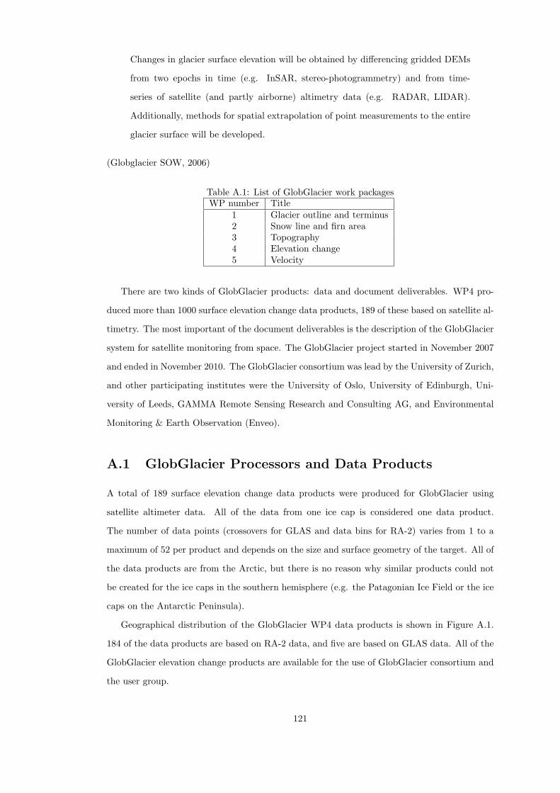
Changes in glacier surface elevation will be obtained by differencing gridded DEMs
from two epochs in time (e.g. InSAR, stereo-photogrammetry) and from time-
series of satellite (and partly airborne) altimetry data (e.g. RADAR, LIDAR).
Additionally, methods for spatial extrapolation of point measurements to the entire
glacier surface will be developed.
(Globglacier SOW, 2006)
Table A.1: List of GlobGlacier work packagesWP number Title
1 Glacier outline and terminus2 Snow line and firn area3 Topography4 Elevation change5 Velocity
There are two kinds of GlobGlacier products: data and document deliverables. WP4 pro-
duced more than 1000 surface elevation change data products, 189 of these based on satellite al-
timetry. The most important of the document deliverables is the description of the GlobGlacier
system for satellite monitoring from space. The GlobGlacier project started in November 2007
and ended in November 2010. The GlobGlacier consortium was lead by the University of Zurich,
and other participating institutes were the University of Oslo, University of Edinburgh, Uni-
versity of Leeds, GAMMA Remote Sensing Research and Consulting AG, and Environmental
Monitoring & Earth Observation (Enveo).
A.1 GlobGlacier Processors and Data Products
A total of 189 surface elevation change data products were produced for GlobGlacier using
satellite altimeter data. All of the data from one ice cap is considered one data product.
The number of data points (crossovers for GLAS and data bins for RA-2) varies from 1 to a
maximum of 52 per product and depends on the size and surface geometry of the target. All of
the data products are from the Arctic, but there is no reason why similar products could not
be created for the ice caps in the southern hemisphere (e.g. the Patagonian Ice Field or the ice
caps on the Antarctic Peninsula).
Geographical distribution of the GlobGlacier WP4 data products is shown in Figure A.1.
184 of the data products are based on RA-2 data, and five are based on GLAS data. All of the
GlobGlacier elevation change products are available for the use of GlobGlacier consortium and
the user group.
121
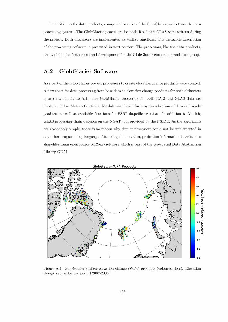
In addition to the data products, a major deliverable of the GlobGlacier project was the data
processing system. The GlobGlacier processors for both RA-2 and GLAS were written during
the project. Both processors are implemented as Matlab functions. The metacode description
of the processing software is presented in next section. The processors, like the data products,
are available for further use and development for the GlobGlacier consortium and user group.
A.2 GlobGlacier Software
As a part of the GlobGlacier project processors to create elevation change products were created.
A flow chart for data processing from base data to elevation change products for both altimeters
is presented in figure A.2. The GlobGlacier processors for both RA-2 and GLAS data are
implemented as Matlab functions. Matlab was chosen for easy visualization of data and ready
products as well as available functions for ESRI shapefile creation. In addition to Matlab,
GLAS processing chain depends on the NGAT tool provided by the NSIDC. As the algorithms
are reasonably simple, there is no reason why similar processors could not be implemented in
any other programming language. After shapefile creation, projection information is written to
shapefiles using open source ogr2ogr -software which is part of the Geospatial Data Abstraction
Library GDAL.
Figure A.1: GlobGlacier surface elevation change (WP4) products (coloured dots). Elevationchange rate is for the period 2002-2008.
122
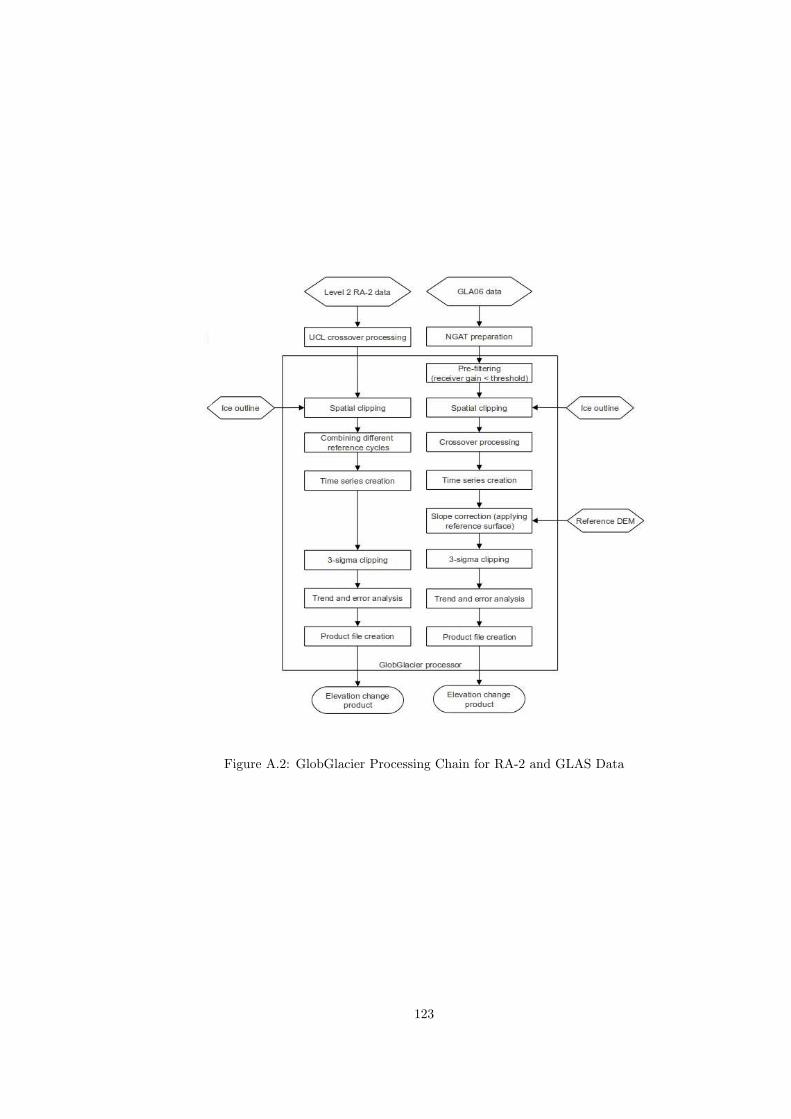
Figure A.2: GlobGlacier Processing Chain for RA-2 and GLAS Data
123
To constrain the elevation change estimates to an ice surface both processors need an ice
outline from an external source. Convenient sources for the outlines are GlobGlacier WP1 and
GLIMS. However, due to large footprint of the RA-2, also coarse outlines from other sources
can be used. A large number of RA-2 products were created with outlines from the Digital
Chart of the World (DCW).
A.2.1 Common functions for RA-2 and GLAS
3-sigma clipping
Elevation points that deviate more than three times the standard deviation from the mean
elevation are discarded.
Spatial clipping
Elevation points falling outside given ice outline are discarded.
Time series creation
All of the elevation measurements from single point in space are combined into one time series
of elevations.
Trend and error analysis
A first degree polynomial is fitted to the time series of elevations. The slope of this polynomial
represents the elevation trend during the observations period. An estimate for uncertainty of
the elevation change is calculated from the sum of residuals between the linear fit and measured
elevations.
Product file creation
Time and elevation vectors, elevation change trend and error estimates are written into an ESRI
shapefile.
A.2.2 RA-2 specific functions
EnviSAT RA2 data as used for GlobGlacier is processed by University College of London (UCL)
Centre for Polar Observation and Modelling from RA2 GDR format Level-2 data.
124
UCL Crossover analysis
The elevations measured by the RA-2 are compared to elevations measured during an orbital
cycle that is chosen as the reference cycle. This method is commonly known as the dual
crossover method. The elevation values are interpolated to orbital crossover points from two
nearest measurements. This produces time series of elevation differences at all orbital crossover
points relative to the reference cycle.
Combining different reference cycles
Elevation difference time series using different reference cycles are combined in to one time
series. This is be done by removing the mean elevation difference from each time series.
A.2.3 ICESat GLAS specific functions
Data used for Ice, Cloud, and land Elevation Satellites (ICESat) Geoscience Laser Altimeter
System (GLAS) elevation change product is the GLAS/ICESat L1B Global Elevation Dataset or
”GLA06” available free of charge online from the National Snow and Ice Data Center (NSIDC).
Pre-filtering
Elevation measurements with elevation gain values larger than given threshold are discarded.
Crossover analysis
An elevation value for orbital crossover point is calculated as the mean of elevations measured
during ascending and descending passes. The elevation can be calculated as the mean of all
measurements falling inside a given radius from the crossover point or the elevation can be
interpolated from subsequent measurements to the exact crossover point. Interpolation is more
precise method of these two and thus recommended.
Slope correction
An external DEM is subtracted from the elevation values. This removes the effect of crossover
points from different operations periods not coinciding and thus including elevation change
induced by the surface slope.
125